Embed Size (px)
Citation preview

OPTIMIZING REINJECTION STRATEGY IN PALINPINON, PHILIPPINES BASED O N CHLORIDE DATA
A REPORT SUBMITTED TO THE DEPARTMENT OF PETROLEUM
ENGINEERING OF STANFORD UNIVERSITY
IN PARTIAL FULFILLMENT OF THE REQUIREMENTS FOR THE DEGREE OF MASTER OF SCIENCE
BY Ma. Elena G. Macario
March 1991

I certify that I have read this report and that in my
opinion it is fully adequate, in scope and in quality, as
partial fulfillment of the degree of Master of Science in Petroleum Engineering.
c - - B1, Roland N. Home
(Principal advisor)
11 ..

Acknowledgements
The years I have spent in Stanford University will always be one of the highlights in
my life and so I would like to offer Dr. Roland N. Home my sincere gratitude for
an abundance of his patience, guidance, and encouragement throughout the course of my stay and this study. He has been, not only a mentor, but also a friend.
I am also thankful to the United Nations Department for Technical Cooperation and Development (UN-DTCD) under whose project PHI/86/006 with the Philippine
National Oil Company - Energy Development Corporation (PNOC-EDC) I was given
the opportunity to pursue a Master’s degree in petroleum engineering. The last years of my study would not have been possible without the financial
assistance provided by the Stanford Geothermal Program under Department of En-
ergy Contract No. DE AS07-84IDI2529 and Grant No. DEFGO7-90IDI2934, and the Department of Petroleum Engineering, Stanford University.
I would like to acknowledge the help of Zim Aunzo, Benjie Aquino, Jim Lovekin, as well as the staff of the Petroleum Engineering Department who have provided me with
warmth and camaraderie. To my husband Ned, I am indebted for his understanding
and support.
To my parents, Benjamin and Norma de Guzman, this work is dedicated with all my love.
111 ...

Abstract
One of the guidelines established for the safe and efficient management of the Palin- pinon Geothermal Field is to adopt a production and reinjection strategy such that
the rapid rate and magnitude of reinjection fluid returns leading to premature thermal
breakthrough would be minimized, if not avoided. To help achieve this goal, sodium
fluorescein and radioactive tracer tests have been conducted to determine the rate
and extent of communication between the reinjection and producing sectors of the
field. The first objective of this work was to examine how the results of these tests, together with information on field geometry and operating conditions could be used in algorithms developed in Operations Research and modified by James Lovekin to allocate production rates among the Palinpinon wells.
Due to operational and economic constraints, however, such tracer tests were very limited in scope and number. This prevents obtaining explicit information on the
interaction between each injection and producing well. Hence, there was a need to look for another parameter which can be used for this purpose. The second objective
of this work was, therefore, to investigate how the reservoir chloride value of the
producing well and the injection rate of the injection well could be used to provide a ranking of the injection/production pair of wells and, thereby, aid in optimizing the reinjection strategy of the field.
iv

1991
Ph.D. DISSERTATIONS
NACUL, Evandro Correa: "Use of Domain Decomposition and Local Grid Refinement in Reservoir Simulation,'' Vols. I and 11. Advisor: Khalid Aziz.
ENGINEERS THESES
GAO, Guozhjeng: "'fie Application of Artificial Intelligence in Well Test Analysis." Advi- sor: Roland N. Home.
MASTER'S REPORTS
MACARIO, Ma. Elena G.: "Optimizing Reinjection Strategy in Palinpinon, Philippines Based on Chloride Data." Advisor: Roland N. Home.
Contents
Acknowledgements iii
Abstract iv
Table of Contents V
List of Tables viii
List of Figures ix
1 Introduction 1
2 Previous Work 4
3 The Palinpinon-I Geothermal Field 6
3.1 Brief Description of Palinpinon-I . . . . . . . , . . . . . . . . . . . . . 6 3.2 Tracer Testing in Palinpinon-I . . . . . . . . . . . . . . . . . . . . . . 8
3.2.1 Sodium Fluorescein Tracer Tests . . . . . . . . . . . . . . . . 8 3.2.2 Radioactive Tracer . . . . . . . . . . . . . . . . . . . . . . . . 9
4 Optimization Strategy 14
4.1 Arc Costs . . . . . . . . . . . . . . . . . . . . . . . . . . . . . . . . . 15 4.2 Linear Programming . . . . . . . . . . . . . . . . . . . . . . . . . . . 18
4.2.1 Transportation Problem . . , . . . . . . . . . . . . , . . . . . 18 4.2.2 Injection Optimization Problem . . . . . . . . . . . . . . . . . 19 4.2.3 LPAL Optimization . . . . . . . . . . . . . . . . . . . . . . . . 21
V
4.3 Quadratic Programming . . . . . . . . . . . . . . . . . . . . . . . . . 23
4.4 Case Results and Discussion . . . . . . . . . . . . . . . . . . . . . . . 23 4.4.1 Sensitivity to Weighting Factors . . . . . . . . . . . . . . . . . 26
4.4.2 Allocation of Production Rates . . . . . . . . . . . . . . . . . 32
5 Use of Chloride Data 36 5.1 Chloride-Flowrate Correlation Method . . . . . . . . . . . . . . . . . 41
5.1.1 PN-9RD Tracer Test Application . . . . . . . . . . . . . . . . 42
5.1.2 Chloride Shift . Flowrate Correlation . . . . . . . . . . . . . . 50
5.1.3 OK-l2RD/PN-GRD Tracer Test Application . . . . . . . . . . 53 5.1.4 Other Production/Reinjection Correlations . . . . . . . . . . . 59
5.2 Chloride . Cumulative Flowrate Correlation . . . . . . . . . . . . . . 72 5.3 Chloride Deviation . Flowrate Correlation . . . . . . . . . . . . . . . 72
5.4 Linear Combination Method . . . . . . . . . . . . . . . . . . . . . . . 80 5.4.1 Results Using Whole Data Set . . . . . . . . . . . . . . . . . . 84
5.4.2 Using the Linear Combination Method in More Detail . . . . 93
6 Conclusions and Recommendation 96
A Production and Injection Zones of Paln-I Wells 99
B Sample Output from Linear Programming 101
C Sample Output from Quadratic Programming 111
D Reservoir Chloride Measurements with Time 115
E Injection Flowrates with Time 126
F C hloride-Flow Correlations 130
G Chloride Shift-Flow Correlation 140
H Chloride-Cumulative Flow Correlation 149
vi

I Chloride Deviation-Flow Correlation
J Chloride Deviation-Flow Program Code
K Linear Combination Program Code and Output
Bibliography
153
161
166
176
vii

List of Tables
3.1 Tracer tests in Palinpinon Geothermal Field . . . . . . . . . . . . . . 13
4.1 Input data for optimization strategy . . . . . . . . . . . . . . . . . . . 25
4.2 A . Sensitivity to different weighting factors . . . . . . . . . . . . . . . 27 4.3 B . Sensitivity to different weighting factors . . . . . . . . . . . . . . . 28
4.4 Ranking of wells using individual weighting factors . . . . . . . . . . . 29 4.5 A . Allocation of production rates to Palinpinon Wells . . . . . . . . . . 33 4.6 B . Allocation of production rates to Palinpinon Wells . . . . . . . . . . 34
5.1 5.2
5.3
5.4
5.5
5.6
5.7 5.8
OK-’I/PN-SRD correlation . . . . . . . . . . . . . . . . . . . . . . . . . 46 PN-9RD selected coefficients of correlation . . . . . . . . . . . . . . . . 48
OK-12RD/PN-GRD selected correlation for first time interval . . . . . 59
Representative coefficients of chloride-flow correlation . . . . . . . . . . 70 Linear combination coefficients for whole data set . . . . . . . . . . . . 85
Comparing tracer tests and the correlation methods . . . . . . . . . . 90
Representative coefficients from the two correlation methods . . . . . . 91 Example of linear combination use . . . . . . . . . . . . . . . . . . . . 94
A.l Production and injection depths . . . . . . . . . . . . . . . . . . . . . 100
... Vlll
List of Figures
3.1 3.2
3.3
4.1 4.2
5.1
5.2
5.3
5.4 5.5 5.6
5.7
5.8 5.9
Location map of the Palinpinon Geothermal Field . . . . . . . . . . . 10 Palinpinon-I surface layout . . . . . . . . . . . . . . . . . . . . . . . . 11 Reservoir chloride vs time . . . . . . . . . . . . . . . . . . . . . . . . 12
Idealized network of arcs . . . . . . . . . . . . . . . . . . . . . . . . . . 15 Ranking of wells with increase in weighting factors . . . . . . . . . . . 31
Palinpinon-I reservoir chloride measurements . . . . . . . . . . . . . . 38 Trend in quartz equilibrium temperatures . (after PNOC.EDC, 1990) 39
Chloride vs flowrate correlation methods . . . . . . . . . . . . . . . . . 40
OK-7 monthly chloride and PN-9RD flowrate . . . . . . . . . . . . . . 43 Using more OK-7 chloride measurements . . . . . . . . . . . . . . . . . 44
Chloride-flow correlation method on OK.’I/PN.gRD . . . . . . . . . . 47 PN-9RD tracer test: chloride . flow correlation . . . . . . . . . . . . . 49
OK-7/PN-9RD chloride shift-correlation method . . . . . . . . . . . . 51 Correlation of injection flowrate with shift in chloride . . . . . . . . . . 52
5.10 PN-17D chloride values and PN-6RD flowrate . . . . . . . . . . . . . . 55
5.11 Chloride-flow correlation method on PN.17D/PN.GRD . . . . . . . . . 56 5.12 OK-12RD/PN-GRD tracer test: chloride-flow correlation . . . . . . . . 58 5.13 PN-6RD correlation with other wells . . . . . . . . . . . . . . . . . . . . 60 5.14 PN-1RD correlation with other wells . . . . . . . . . . . . . . . . . . . 62
5.15 PN-2RD correlation with other wells . . . . . . . . . . . . . . . . . . . 63 5.16 PN-3RD correlation with other wells . . . . . . . . . . . . . . . . . . . 64
5.17 PN-4RD correlation with other wells . . . . . . . . . . . . . . . . . . . 65
ix
5.18 PN-5RD correlation with other wells . . . . . . . . . . . . . . . . . . . 66
5.19 PN-7RD correlation with other wells . . . . . . . . . . . . . . . . . . . 67
5.20 PN-8RD correlation with other wells . . . . . . . . . . . . . . . . . . . 68
5.21 PN-9RD correlation with other wells . . . . . . . . . . . . . . . . . . . 69 5.22 Chloride-cumulative flow correlation method on OK.7/PN.9RD . . . . 73
5.23 Chloride-cumulative flow correlation method on PN.17D/PN.GRD . . 74
5.24 Selected chloride-cumulative flow correlations . . . . . . . . . . . . . . 75 5.25 Ch1o:ride and deviation of chloride from best fit line . . . . . . . . . . . 77 5.26 Ch1o:ride deviation-flow correlation method on OK.7/PN.9RD . . . . . 78
5.27 PN-SRD tracer test: comparing two chloride-flow methods . . . . . . . 79
5.28 Chloride deviation-flow correlation method on PN.17D/PN.GRD . . . 81
5.29 OK-]L2RD/PN-GRD tracer test: comparing two chloride-flow methods . 82 5.30 Linear combination coefficients featuring production wells . . . . . . . 86
5.31 Linear combination coefficients featuring injection wells . . . . . . . . . 87 5.32 Chloride-flow correlations featuring reinjection wells . . . . . . . . . . 92
D.l OK-7/OK-9D Reservoir chloride with time . . . . . . . . . . . . . . . . 116
D.2 OK-lIOD/PN-14 Reservoir chloride with time . . . . . . . . . . . . . . 117 D.3 PN-I5D/PN-l6D Reservoir chloride with time . . . . . . . . . . . . . . 118
D.4 PN-I7D/PN-l8D Reservoir chloride with time . . . . . . . . . . . . . . 119
D.5 PN-I.SD/PN-20D Reservoir chloride with time . . . . . . . . . . . . . . 120 D.6 PN-21D/PN-23D Reservoir chloride with time . . . . . . . . . . . . . . 121 D.7 PN-f!4D/PN-26 Reservoir chloride with time . . . . . . . . . . . . . . . 122 D.8 PN-27D/PN-28 Reservoir chloride with time . . . . . . . . . . . . . . . 123
D.9 PN-29D/PN-30D Reservoir chloride with time . . . . . . . . . . . . . . 124
D.10 PN-31D Reservoir chloride with time . . . . . . . . . . . . . . . . . . . 125
E.l PN-I.RD/PN-2RD/PN-SRD Injection flowrates with time . . . . . . . 127
. E.2 PN-4RD/PN-5RD/PN-GRD Injection flowrates with time . . . . . . . 128 E.3 PN-TRD/PN-SRD/PN-SRD Injection flowrates with time . . . . . . . 129
F.l PN-ILRD Chloride-flow correlations with time . . . . . . . . . . . . . . 131
X
F.2 PN-2RD Chloride-flow correlations with time . . . . . . . . . . . . . . 132 F.3 PN-3RD Chloride-flow correlations with time . . . . . . . . . . . . . . 133 F.4 PN-4RD Chloride-flow correlations with time . . . . . . . . . . . . . . 134 F.5 PN-5RD Chloride-flow correlations with time . . . . . . . . . . . . . . 135 F.6 PN-6RD Chloride-flow correlations with time . . . . . . . . . . . . . . 136
F.7 PN-7RD Chloride-flow correlations with time . . . . . . . . . . . . . . 137
F.8 PN-8RD Chloride-flow correlations with time . . . . . . . . . . . . . . 138 F.9 PN-9RD Chloride-flow correlations with time . . . . . . . . . . . . . . 139
G.l G.2 G.3
G.4
G.5 G.6
G.7
G.8
OK-7 chloride shift-flow correlation . . . . . . . . . . . . . . . . . . . 141 OK-7 chloride shift-flow correlation . . . . . . . . . . . . . . . . . . . 142 PN-26 chloride shift-flow correlation . . . . . . . . . . . . . . . . . . . 143
PN-26 chloride shift-flow correlation . . . . . . . . . . . . . . . . . . . 144
PN-28 chloride shift-flow correlation . . . . . . . . . . . . . . . . . . . 145 PN-29D chloride shift-flow correlation . . . . . . . . . . . . . . . . . . 146
PN-SOD chloride shift-flow correlation . . . . . . . . . . . . . . . . . . 147
PN-31D chloride shift-flow correlation . . . . . . . . . . . . . . . . . . 148
H.l Chloride-cumulative flow correlation . . . . . . . . . . . . . . . . . . . 150 H.2 Chloride-cumulative flow correlation . . . . . . . . . . . . . . . . . . . 151
H.3 Chloride-cumulative flow correlation . . . . . . . . . . . . . . . . . . . 152
1.1 PN-1RD Chloride deviation-flowrate correlation . . . . . . . . . . . . . 154
1.2 PN-2RD Chloride deviation-flowrate correlation . . . . . . . . . . . . . 155
1.3 PN-3RD Chloride deviation-flowrate correlation . . . . . . . . . . . . . 156
1.4 PN-4RD Chloride deviation-flowrate correlation . . . . . . . . . . . . . 157
1.5 PN-5RD Chloride deviation-flowrate correlation . . . . . . . . . . . . . 158 1.6 PN-7RD Chloride deviation-flowrate correlation . . . . . . . . . . . . . 159 1.7 PN-8RD Chloride deviation-flowrate correlation . . . . . . . . . . . . . 160
xi

Section 1
Introduction
This study aimed at finding ways of optimizing the production and well utilization scheme at the Palinpinon-I Geothermal steamfield. In a geothermal field exploitation,
the main objective is to provide a balance between obtaining maximum productivity
from the wells and, at the same time, prolonging the economic life of the reservoir. Presently, the developer relies on a variety of ways ranging from experimental methods to numerical simulation to help ensure that the field is being managed safely and
efficiently. Depending on field response, appropriate development strategies and field management policies are instituted and modified.
The Palinpinon Geothermal Field is one of two producing steamfields currently op- erated by the Philippine National Oil Company (PNOC). Even in the early stages of drilling, the importance of injection to dispose of wastewater while maintaining reser-
voir pressures has been recognized. Hence, the steam requirement of the 112.5 MWe
commercial plant, known as Palinpinon-I, is met by 21 production wells and 10 rein-
jection wells drilled as deep and as far away as possible from the producing wells. The production wells produce from multiple feed zones and discharge two-phase fluid
from a liquid-dominated reservoir. Being a variable load power station, Palinpinon-I was operated at low loads dur-
ing the first few years of operation as the transmission lines and distribution system for the Negros Island were being completed. As a result, production and reinjection
wells were util.ized intermittently, affording adequate surface and well testing exercises
1

SECTION I. INTRODUCTION 2
which showed the fast response of the field to exploitation. One of the more signif- icant changes observed was the general trend of increasing reservoir chloride among the producing wells. This has been attributed mainly to the rapid returns of reinjec-
tion fluids to the producing sector (Harper and Jordan, 1985). Apprehensive of the
negative effects of rapid reinjection returns, such as premature thermal degradation
of producing wells, developers implemented guidelines for the safe and efficient man- agement of the Palinpinon reservoir. One of these is adoption of a production and reinjection well utilization strategy, under any given load demand, such that the rapid
rate and magnitude of reinjection fluid returns would be minimized, if not avoided. Presently, decisions on well utilization schemes have been arrived at, on a relative basis, by the confluence of production and reinjection fluid chemistry, downhole mea- surements of pressure and temperature, interference testing , tracer testing, and the
interpreted field model.
The necessity of providing a tool to optimize the well utilization strategy has
served as the primary motivation for this work. To achieve this goal, the problem
has to be posed as an optimization problem. Firstly, this means defining the set of independent variables or parameters and the constraints which are the conditions or restrictions that limit the acceptable values of the variables. Secondly, this ne- cessitates forming an objective function related in some way to the variables. The
solution of the optimization problem is a set of allowed values of the variables for
which the objective function, after maximizing or minimizing assumes the “optimal” value. Finally, to solve the formulated optimization problem, algorithms should be
selected and modified. This has been the approach taken by James Lovekin (1987) in
his work where injection scheduling in geothermal fields was optimized using tracer data. Flowrates are the variables subject to well and field operating conditions, and the fieldwide breakthrough index has been defined as the objective function.
This work applied the algorithms developed and modified by James Lovekin to
the Palinpinon-I tracer return data, along with field geometry and well/field con- straints. However, since Palinpinon tracer tests were limited in scope and number,
an exhaustive producer/injector interaction can not be obtained. There was a need,
therefore, to find another parameter that could be used to relate producer to injector
SECTION 1. INTRODUCTION 3
for use in the optimization algorithms. It was natural to turn to reservoir chloride as
one such parameter since chloride had always been used to infer the extent and mag-
nitude of reinjection returns to the producing sector from the injection wells. Four different methods were tested to determine the degree of correlation or the strength of the relationship between the chloride value of a producing well and the flowrate
of an injection well. The first three calculate the correlation between a particular producer/injector pair of wells at any given time, while the last method expresses the chloride value of a producer as a linear combination of the flowrates of the all the
injection wells in service for the particular time interval considered.
Following this brief introduction, the second section of this report discusses pre- vious work along this line of geothermal field optimization. A brief discussion of the
Palinpinon Geothermal Field is given in the third section. The methods and results of optimization strategy using linear and quadratic programming are presented in
the fourth section. The fifth section describes and applies the different methods of using chloride to obtain producer/injector coefficients of correlation. Finally, the last section summarizes the conclusions from this study and suggests methods of improve- ment.

Section 2
Previous Work
To date, the author is cognizant of only the work of James Lovekin (1987) along
the line of geothermal optimization. In his study, Lovekin has made an exhaustive search of literature to determine what has been done to study the effects of injection
in geothermal fields. Though the two usual approaches to this problem are analytical and numerical modeling of the reservoirs, these are hampered by the inherent difficulty of contructing realistic models due to fracturing and non-isothermal conditions in the
reservoir. Therefore, developers turn to the more powerful and practical method of
tracer testing to determine the behavior of injected fluid. In his work, Lovekin made use of these available tracer return data to correlate the
tracer results with the potential for thermal breakthrough. The underlying foundation is the simplici.ty with which the reservoir is idealized as a network of arcs connecting each pair of wells, and associating with each pair of wells an index which gives a
measure of the magnitude of the flow of fluid from one well to another. Hence, by
defining a function that is to be minimized, the problem has been transposed into
one of optimization.
This study applies the results of Lovekin’s to see how the Palinpinon-I would allocate production and injection rates on the basis of tracer test results. However, as Lovekin has demonstrated, the program works best when there is explicit information
that relates every pair of wells. Since this is not true for the Palinpinon case, a method
has to be found that would express the strength of relationship between producer and
4

SECTION 2. PREVIOUS WORK 5
injector and be used in the optimization routines. This is where the study departs from Lovekin’s work.

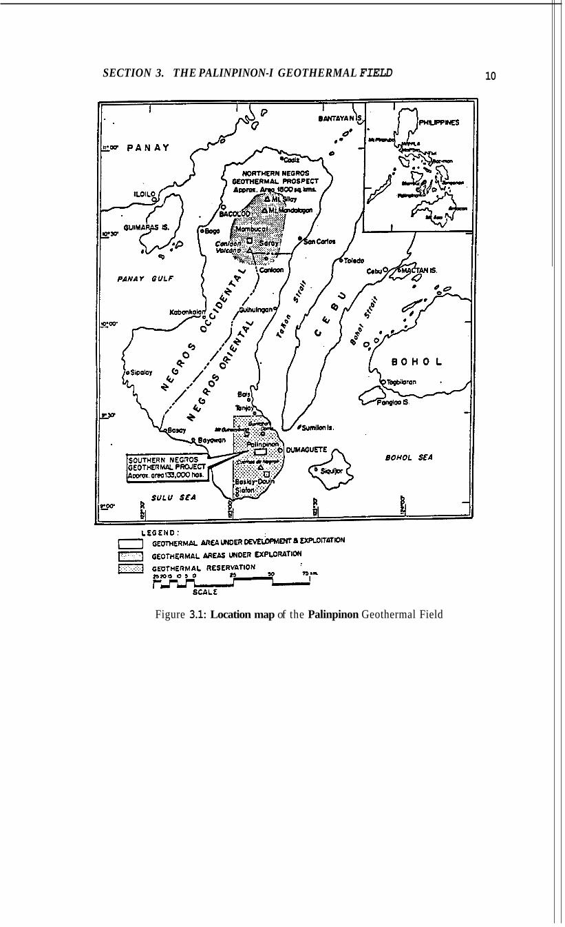
Section 3
The Palinpinon-I Geothermal Field
The Palinpinon Field (Figure 3.1) and the Baslay de Dauin field are the two geother- mal fields comprising the Southern Negros Geothermal Project. The Palinpinon field is situated roughly 15 kms. west of the coastal city of Dumaguete, the provincial
government of Negros Oriental. It is divided into two sectors - the Puhagan sector in the east and Nasuji/Sogongon in the west. The Puhagan sector, which is the con-
cern of this study, has the first large plant, Palinpinon-I, with a generating capacity
of 112.5 MWe while the Nasuji/Sogongon sector has been alloted for the proposed
development of Palinpinon-11.
3.1 Brief Description of Palinpinon-I
Palinpinon-I is one of two steamfields currently operated by the Philippine National Oil Company (PNOC). The power station, unlike most other geothermal power sta-
tions, was designed and constructed to operate as a variable load station. Due to
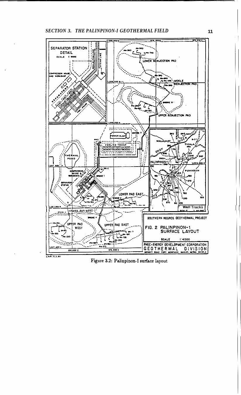
the hostile topography of the area, a compact development scheme consisting of four multi-well production pads and three multi-well injection pads was effected. Fig-
ure 3.2 shows' the steam gathering system, the well pads, as well as the well tracks.
6
SECTION 3. THE PALINPINON-I GEOTHERMAL FIELD 7
Eighteen (18) of the twenty-one (21) production wells were drilled directionally to in-
tersect structures which were believed to be zones of high permeability. These wells, drilled to depths ranging from 2774 mMD (measured depth) to 3467 mMD produce from multiple zones and discharge two-phase fluid from a single-phase reservoir.
The need to reinject waste liquid effluent has been primarily dictated by envi-
ronmental constraint, which in the Philippines prohibits full disposal into the rivers being used for ricefield irrigation. In addition, the benefits of maintaining reservoir pressures and increasing thermal recovery through reinjection have been recognized.
The ten (10) reinjection wells which accept waste liquid by gravity flow, were drilled
to the eastern, northern, and western sections of the sector. They have been drilled as deep and as far as possible, at the periphery of the field identified to be the outflow region of the reservoir.
Shortly after commissioning of the Palinpinon-I power plant in June 1983, ini-
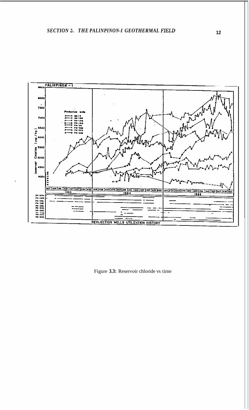
tial observations of the reservoir response and performance of both production and
reinjection well showed significant changes. One of these was the increasing trend of reservoir chloride for the production wells (Figure 3.3). This has been interpreted (Harper and Jordan, 1985) as evidence of the rapid return of reinjected fluids to
the producing sector, and in some cases, to localized pressure drawdown. Since this could lead to premature thermal breakthrough of cooler injected fluids at producing wells, and cut short the economic life of the field, guidelines for the safe and efficient
management of the Palinpinon reservoir have been established. These include the requirements of
0 minimizing fluid residence times in the surface and downhole piping while op- erating reinjection wells at or near maximum capacity,
0 minimizing steam wastages brought about by varying steam demand and supply, and
0 adopting a production and reinjection well utilization strategy such that the
rapid rate and magnitude of reinjection fluid returns leading to premature ther- mal breakthrough would be minimized, if not avoided.

SECTION 3. THE PALINPINON-I GEOTHERMAL FIELD 8
The first of these requirements is the solution to the problem of silica deposition
which would occur by gravity injection of a fluid that is supersaturated with respect
to amorphous silica. The second requirement which is economical in nature, has been
satisfied by prioritizing high enthalpy production wells for peaking steam requirements
and choosing injection wells with additional capacity. Presently, decisions on well
utilization schemes have been arrived at, on a relative basis, by the confluence of production and reinjection fluid chemistry, downhole measurements of pressure and temperature, interference testing, tracer testing, and the interpreted field model. This study attempts to provide another tool to identify fast injection paths, and aid in
optimizing the well utilization strategy.
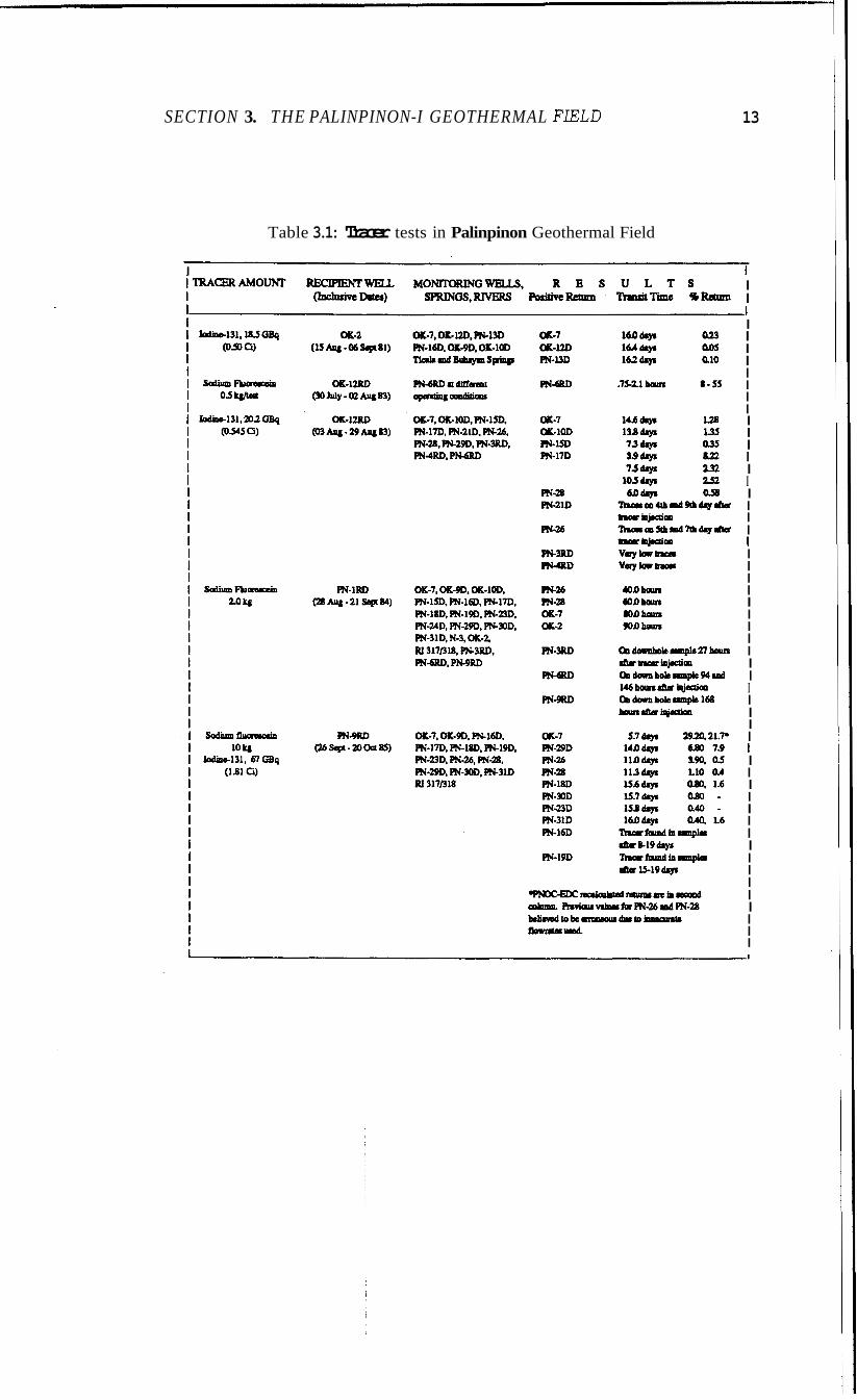
3.2 Tracer Testing in Palinpinon-I
To determine the rate and extent of communication between a reinjection well (or
sector), and the producing area, tracer tests were conducted in Palinpinon-I. These
tests and the results are shown in Table 3.1.
3.2.1 Sodium Fluorescein Tracer Tests
The first chemical tracer tests used the organic dye sodium fluorescein, which was introduced in July 1983 to investigate the interconnection between OK-12RD and PN-6RD. Direct connection between the two was confirmed by visual inspection of
the fluid sample just 1.5 hours after injection.
In August 1984, a year after commercial operation began, the chemical dye was
used on a larger scale to determine interaction of well PN-1RD with the production sector. Sixteen (16) of the production wells were monitored but positive return of the tracer (detected through UV light spectrophotometer) was confirmed only for the central Puhagan wells PN-26, PN-28, OK-7, as well as at OK-2. Arrival times ranged from 40 to 90 hours - equivalent to breakthrough velocities of 5.6 to 16.5
m/hr. Tracer return in other wells could not be ascertained due to interference of
degraded by-products of sodium fluorescein with the viewing process.
SECTION 3. THE PALINPINON-I GEOTHERMAL FIELD 9
Another year later, in August 1985, a greater amount of the dye was injected in PN-9RD as a precursor to the radioactive tracer testing. The test aimed to define communication between the western injection sector and the producing area. In a
day’s time, the dye was seen in OK-7 produced fluid. Arrival times for wells PN-l7D,
PN-19D, PN-26, PN-28, PN-29D and PN-31D ranged from 5.5 to 6.0 days, while for
the more distant production wells PN-16D, PN-23D, and PN-SOD, first appearance
of the chemical tracer occured in 7.5 to 9.8 days.
3.2.2 Radioactive Tracer
The radioactive tracer Iodine-131 (I 131) was used to be able to detect even minute
returns of the injected tracer.
The first radioactive tracer was conducted in August 1981 to investigate movement
of fluid injected into a shallow well to adjacent but much deeper wells. The miniscule
return discounted any large direct connection between OK-2 and the adjacent wells.
In August 1983, the OK-12RD radioactive tracer test confirmed direct communi- cation between the eastern injection well OK-12RD and the eastern production wells PN-17D, PN-l5D, PN-21D, and OK-1OD in addition to the central Puhagan wells
OK-7, PN-28, and PN-26. Estimated total return was 17% with mean transit times of 4 to 15 days. These translate to average aerial flow velocities of 1.7 to 4.6 m/hr. Still, the result indicates that a greater portion of the injected fluid was dispersed
away from the producing sector.
Shortly after monitoring of the sodium fluorescein dye in PN-SRD, a four-fold increase of 1-131 was injected into PN-9RD. The result affirmed the fast and strong
returns to OK-7 with breakthrough time of a day, mean transit time of 5.7 days, and tracer recovery of approximately 30%. The mean transit time is the time it takes for
half of the tracer return to reach the production well. The rest of the production wells
had tracer returns of 0.4% to 7% and average transit times of 10.3 to 16.0 days. The
total tracer recovery of 45% indicates that more reinjection fluid was now returning to the producing block than had been the case before commercial operation. It affirmed
the backtracking of injected fluid from the western injectim sector to the central, western and southwestern producting areas.
SECTION 3. THE PALINPINON-I GEOTHERMAL FIELD 10
Figure 3.1: Location map of the Palinpinon Geothermal Field
SECTION 3. THE PALINPINON-I GEOTHERMAL FIELD 11
I I
Well Tracks LICALC 1.40.000
- P
\ 60tX
E
‘6 L
c 4% 3 a
SECTION 3’. THE PALINPINON-I GEOTHERMAL FLELD 12
ALINPINoN - It .. ,
I - --
Figure 3.3: Reservoir chloride vs time
SECTION 3. THE PALINPINON-I GEOTHERMAL FlELD 13
Table 3.1: Tracer tests in Palinpinon Geothermal Field
I 1 I I .I I I I I I I I I I I I I I I I I I I I I I I I I I I I I I I I I I I I 1 I I I I I I I I I I I I I I I I

Section 4
Optimization Strategy
The results of the two tracer tests, together with field geometry, and field operating conditions were used to test algorithms developed and modified by James Lovekin (1987) to allocate production rates among the Palinpinon wells. This section gives
a brief discussion on the fundamentals of the methods used to optimize reinjection
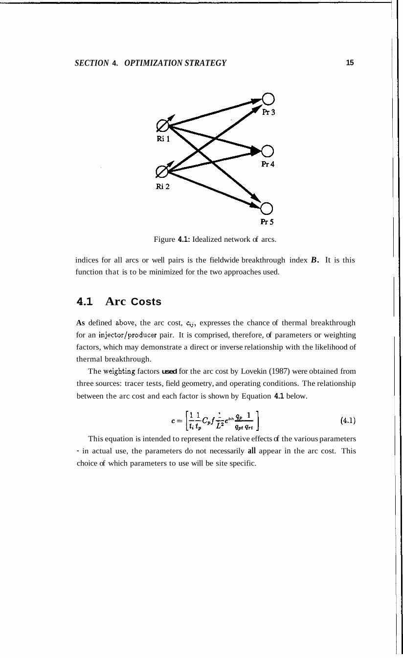
and production rates. The reader is referred to Lovekin (1987) for a more thorough
discussion of the algorithms and the differences between the programs used for each method.
The optimization strategy is analogous to the classical transportation problem, where a set of factories supplies a set of stores. The problem is to determine the optimum distribution scheme for the goods using the various routes or arcs such that the total transportation cost is minimized and the constraints of factory capacity,
as well as store requirements are satisfied. In the geothermal analogy, the factories
are the injection wells and the stores are the producers. The geothermal reservoir is idealized as a network of arcs between every pair of well where each arc is presupposed to have some potential for thermal breakthrough caused by the flow of fluid from
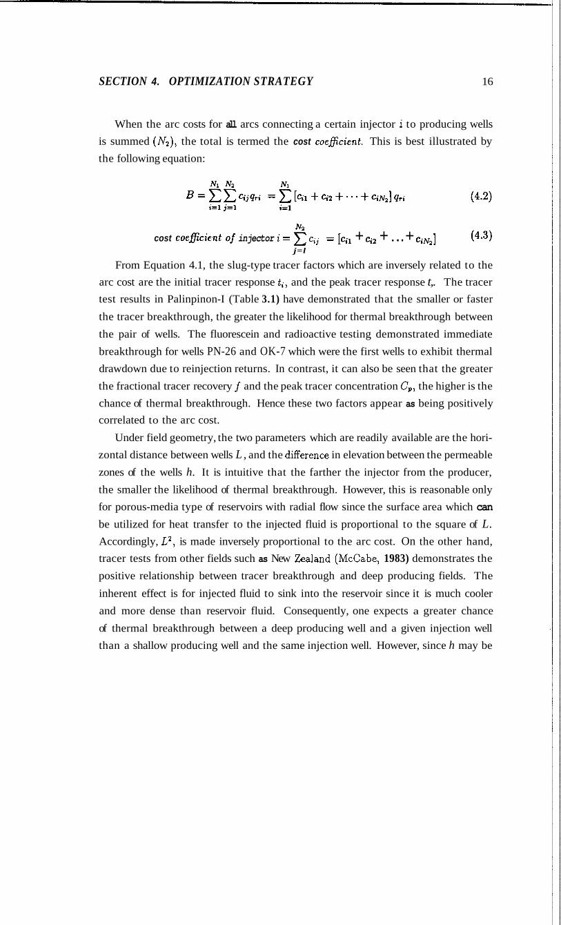
injector to producer (Figure 4.1). This increased chance of thermal breakthrough is measured by the arc cost, Gj,
and the product of the arc cost with the well’s injection rate, qr;, is defined as the
injector/producer pair breakthrough index, b;j. The sum of an injector’s arc costs
over all the producing wells is its cost coeficient , and the sum of the breakthrough
14
SECTION 4. OPTIMIZATION STRATEGY 15
W Pr5
Figure 4.1: Idealized network of arcs.
indices for all arcs or well pairs is the fieldwide breakthrough index B. It is this function that is to be minimized for the two approaches used.
4.1 Arc Costs
As defined a.bove, the arc cost, q j , expresses the chance of thermal breakthrough for an injector/producer pair. It is comprised, therefore, of parameters or weighting factors, which may demonstrate a direct or inverse relationship with the likelihood of thermal breakthrough.
The weig:hting factors used for the arc cost by Lovekin (1987) were obtained from three sources: tracer tests, field geometry, and operating conditions. The relationship
between the arc cost and each factor is shown by Equation 4.1 below.
bh q P
This equation is intended to represent the relative effects of the various parameters - in actual use, the parameters do not necessarily all appear in the arc cost. This
choice of which parameters to use will be site specific.
SECTION 4. OPTIMIZATION STRATEGY 16
When the arc costs for all arcs connecting a certain injector i to producing wells is summed (NZ), the total is termed the cost coeficient. This is best illustrated by the following equation:
N2 cost coeficient of injector i = cij = [til + ci2 + . . . + c ;Nz] (4.3)
j=l
From Equation 4.1, the slug-type tracer factors which are inversely related to the arc cost are the initial tracer response t;, and the peak tracer response t,. The tracer test results in Palinpinon-I (Table 3.1) have demonstrated that the smaller or faster
the tracer breakthrough, the greater the likelihood for thermal breakthrough between
the pair of wells. The fluorescein and radioactive testing demonstrated immediate
breakthrough for wells PN-26 and OK-7 which were the first wells to exhibit thermal drawdown due to reinjection returns. In contrast, it can also be seen that the greater
the fractional tracer recovery f and the peak tracer concentration C,, the higher is the chance of thermal breakthrough. Hence these two factors appear as being positively correlated to the arc cost.
Under field geometry, the two parameters which are readily available are the hori- zontal distance between wells L , and the difference in elevation between the permeable
zones of the wells h. It is intuitive that the farther the injector from the producer,
the smaller the likelihood of thermal breakthrough. However, this is reasonable only for porous-media type of reservoirs with radial flow since the surface area which can be utilized for heat transfer to the injected fluid is proportional to the square of L. Accordingly, L2, is made inversely proportional to the arc cost. On the other hand, tracer tests from other fields such as New Zealand (McCabe, 1983) demonstrates the
positive relationship between tracer breakthrough and deep producing fields. The
inherent effect is for injected fluid to sink into the reservoir since it is much cooler
and more dense than reservoir fluid. Consequently, one expects a greater chance
of thermal breakthrough between a deep producing well and a given injection well than a shallow producing well and the same injection well. However, since h may be
SECTION 4. OPTIMIZATION STRATEGY 17
positive or negative depending on whether the producing zone is below or above the
injection zone, it is not suitable as a weighting factor. The elevation difference h is
considered positive when the producing zone is below the injecting zone. To be used
as a weighting factor, Lovekin (1987) included ti as an ,exponential function e'", with
a scaling factor s to prevent the exponential term from dominating the rest of the
weighting factors. This report maintains the 0.001 value for s to keep the weight- ing factor within the range of 0.37 to 2.72 for elevation differences on the order of hundreds of meters (Lovekin, 1987).
Flow rates for production and injection wells during the tracer tests (qpt and qrt)
can also be included as weighting factors. A well producing at a low rate with a positive return can be expected to encounter earlier breakthrough than another well
producing at a higher rate with similar returns. Such is the case for PN-26 during
the PN-9RD tracer test. The actual tracer return to PN-26 is only about 0.5 since it
was on heavy bleed during the tracer testing. This value is comparable to the returns (0.8 - 0.4) from the other wells (Table 3.1) which were producing at higher rates. Consequently, it is to be expected that had PN-26 been producing at a higher rate during tracer testing qrt, then its tracer returns would be much higher, indicative of
an an earlier breakthrough. Subsequent field experience has proven that this is so.
The same reasoning would apply to the injection rate qrt. Therefore, these parameters enter as reciprocals in the calculation for arc cost.
In Equation 4.1, the producing rate under operating conditions qp has been en- tered as a weighting factor with linear relationship to the arc cost. Ideally, higher
production mtes cause greater pressure drawdown and increase the likelihood of ther-
mal breakthrough. The inclusion of the producing rates under operating conditions as
weighting factors rather than decision variables is based on the assumption that these
rates are predetermined based on total production requirements. If this is not the
case, and qp is a decision variable, the ratio qp/qpt can be viewed as being proportional to the breakthrough index b. When the injection rate under operating conditions qT,
is a decision variable, then the ratio qr/qrt can be regarded in a similar manner. The
greater these ratios are, the higher the possibilities for thermal breakthrough.
It is to be emphasized again that all these weighting factors need not be used
SECTION 4. OPTIMIZATION STRATEGY 18
to calculate the arc cost. Likewise, the combination of these factors is not intended
to be exhaustive. Other weighting factors that the developer may deem as or more important on the basis of reservoir information and behaviour can be and should be included. Finally, appropriate weights or scaling factors could be affixed to the other arc cost components as well.
4.2 Linear Programming
A linear programming problem is a mathematical program in which the objective function is linear in the unknowns and the constraints consist of linear equalities and inequalities (Luenberger, 1984).
4.2.1 Transportation Problem
In the transportation problem, it is desired to ship quantities al, a2,. . . ,a; , respec-
tively of a certain product or goods from each of i factories and received in amounts bl, b, .. . , bj, respectively, at each of j destinations or stores. Associated with the transporting of a unit of product from origin or factory i to destination or store j is a
unit transportation cost, c;j. It is desired to determine the amounts x;j to be shipped
between each factory-store pair i = 1 ,2 , . . . , N,; j = 1 , 2 , . . . , Nz; so as to satisfy the
shipping requirements and minimize the total cost of transportation, C. Hence, the formulation of the transportation problem is given by Equation 4.4.
Minimize
Subject to
x;j = bj, i=1
i = l , N1
j=1, NZ
for all i, j
SECTION 4. OPTIMIZATION STRATEGY 19
As seen in Equation 4.4 and its constraints, the classic transportation problem
satisfy the requirements of a linear programming problem which is then solved, usu-
ally, by an algorithm such as the Simplex method. As a start, in the optimization problem, the decision variables are the injection rates because it was assumed that production rates had been determined beforehand.
4.2.2 Injection Optimization Problem
The formulation of the injection optimization problem is given by Equation 4.5 below. Minimize
NI Nz NI N2 B = C b i j = r x c ; j q r ; (4.5)
i=l j=1 i=l j=1
Subject to Qri h grimax, i = l , NI
fi: i= l
qr; Q r t d
The injection optimization problem has the following features which demonstrate
its resemblance to the transportation problem.
1. The decision variables, qri are the injection rates for each injection well i instead of the amount of goods transported from factory i to store j.
2. The arc costs, c i j , expressing the chance of thermal breakthrough for each in-
jector/producer arc or flow path replace the transportation costs per unit of goods shipped.
3. The objective function to be minimized is the fieldwide breakthrough index in
place of the total transportation cost.
4. The supply constraint for a factory is now supplanted by the requirement that each injector should operate at a rate less than its capacity, grimax.
SECTION 4. OPTIMIZATION STRATEGY 20
5. The demand constraint for a store is now denoted by the requirement that the summation of all injection rates be equal to the specified fieldwide total injection
rate, Qrfot . And,
6. The non-negativity constraint requiring that goods be shipped only from factory
to store, correspond to demanding that the injectors not act as producers by
operating at a "negative rate".
Although the preceding discussion outlines the similarity between the transporta- tion problem and the injection optimization problem, there exists differences between the two.
1. While the transportation problem solves for the amount of goods shipped ucross
each arc, the optimization problem solves for injection rates ut each injection well. Hence, the first is arc-specific while the latter is well-specific. This is
natural since the geothermal developer does not have direct control over the paths of injected fluids.
2. Whereas the supply constraint in the transportation problem requires that the total of ,goods supplied by a factory i be less than or equal to its capacity, there is no need to sum the reinjection rates into each injection well in the optimization
problem since the rate already delineates all flows away from the well.
3. While the demand constraint in the transportation problem requires that the
sum of goods received by store j be greater than or equal to its demand, this
constraint in the optimization problem is dictated, rather, by the total injection rate demanded of the field as perceived by the developer.
4. Although the transportation problem demands a material balance between the
amount of goods shipped and received, there is no such requirement between the sum of injection rates and the sum of production rates. After all, as the
developer decides, reinjected fluid can be part of or greater than production.
SECTION 4. OPTIMIZATION STRATEGY 21
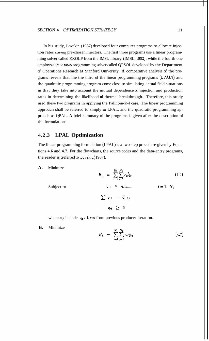
In his study, Lovekin (1987) developed four computer programs to allocate injec- tion rates among pre-chosen injectors. The first three programs use a linear program- ming solver called ZXOLP from the IMSL library (IMSL, 1982), while the fourth one employs a quadratic programming solver called QPSOL developed by the Department of Operations Research at Stanford University. A comparative analysis of the pro-
grams reveals that the the third of the linear programming programs (LPALS) and
the quadratic programming program come close to simulating actual field situations
in that they take into account the mutual dependence of injection and production
rates in determining the likelihood of thermal breakthrough. Therefore, this study
used these two programs in applying the Palinpinon-I case. The linear programming approach shall be referred to simply as LPAL, and the quadratic programming ap- proach as QPAL. A brief summary of the programs is given after the description of the formulations.
4.2.3 LPAL Optimization
The linear programming formulation (LPAL) is a two step procedure given by Equa-
tions 4.6 and 4.7. For the flowcharts, the source codes and the data-entry programs, the reader is :referred to Lovekin( 1987).
A. Minimize
Subject to qri L qrimax,
where c;j includes q,j-term from previous producer iteration.
B. Minimize
SECTION 4. OPTIMIZATION STRATEGY 22
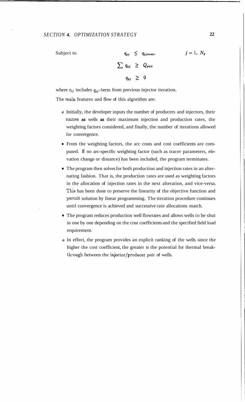
Subject to j = 1 , NZ
where ci, includes qpj-term from previous injector iteration.
The madn features and flow of this algorithm are:
0 Initially, the developer inputs the number of producers and injectors, their
na:mes as wells as their maximum injection and production rates, the weighting factors considered, and finally, the number of iterations allowed for convergence.
0 From the weighting factors, the arc costs and cost coefficients are com-
puted. If no arc-specific weighting factor (such as tracer parameters, ele-
vation change or distance) has been included, the program terminates.
0 The program then solves for both production and injection rates in an alter- nating fashion. That is, the production rates are used as weighting factors in the allocation of injection rates in the next alteration, and vice-versa.
This has been done to preserve the linearity of the objective function and pe:rmit solution by linear programming. The iteration procedure continues until convergence is achieved and successive rate allocations match.
0 The program reduces production well flowrates and allows wells to be shut in one by one depending on the cost coefficients and the specified field load
requirement.
0 In effect, the program provides an explicit ranking of the wells since the higher the cost coefficient, the greater is the potential for thermal break-
thlrough between the injector/producer pair of wells.
SECTION 4. OPTIMIZATION STRATEGY 23
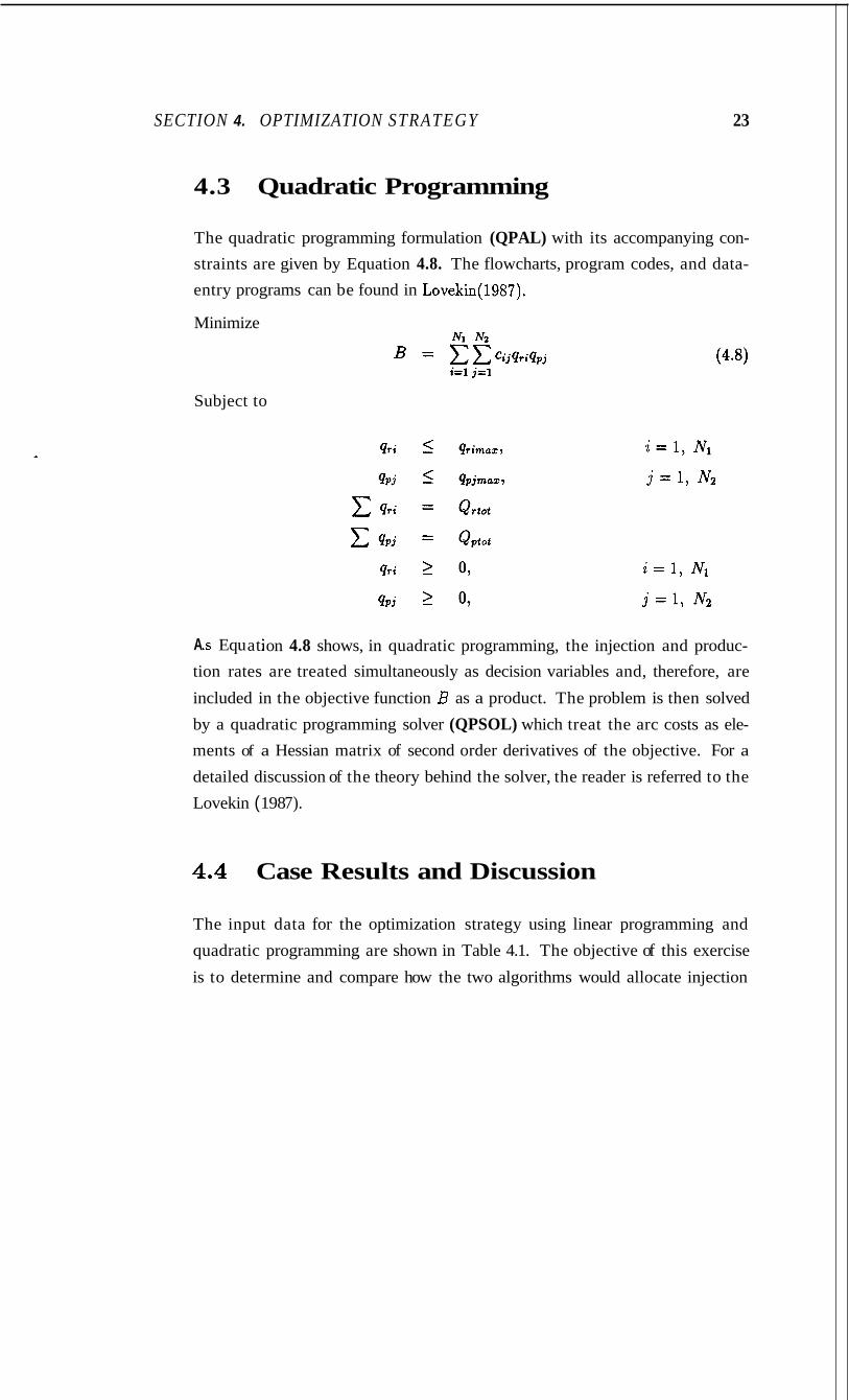
4.3 Quadratic Programming
The quadratic programming formulation (QPAL) with its accompanying con- straints are given by Equation 4.8. The flowcharts, program codes, and data- entry programs can be found in Lovekin(l987).
Minimize
Subject to
A .s Equ at j
i = l , NI
j = 1 , N2
i = l , N1
j = 1 , N2
on 4.8 shows, in quadratic programming, the injection and produc- tion rates are treated simultaneously as decision variables and, therefore, are
included in the objective function B as a product. The problem is then solved
by a quadratic programming solver (QPSOL) which treat the arc costs as ele- ments of a Hessian matrix of second order derivatives of the objective. For a
detailed discussion of the theory behind the solver, the reader is referred to the
Lovekin ( 198 7).
4.4 Case Results and Discussion
The input data for the optimization strategy using linear programming and
quadratic programming are shown in Table 4.1. The objective of this exercise
is to determine and compare how the two algorithms would allocate injection
SECTION 4. OPTIMIZATION STRATEGY 24
rates between the two injection wells and production rates among the different
Palinpinon-I production wells. Only the results of the radioactive tracer tests
are used because the parameters available from the sodium fluorescein tests are not sufficient. To illustrate, only the,breakthrough times of the dye were quantified during the Palinpinon fluorescein tracer tests.
For the radioactive tracer tests, the parameters used as weighting factors for the arc cost are the mean transit time, t, and the fractional recovery f. Due to the inherent limitation of tracer tests, some of the tracer parameters may
not be known or can not be obtained for some injector/producer pairs. As
an example, there may be no tracer return on some monitored wells or some
producing wells had not been monitored due to operational constraints. In the
first case of no positive return, parameters which are directly proportional to thermal breakthrough, such as C, or f, are entered as zeros. This calculates a
zero arc cost which signifies the absence of thermal breakthrough along this arc. To prevent division by zero for parameters such as t , or t , which are inversely
related to thermal breakthrough, arbitrarily large numbers had been entered
to produce negligibly small arc costs. For the second case where tracer data
are missing or lacking, the tracer parameters are entered in a similar fashion
as the first. This is a drawback of the program, since it can not distinguish
between no response and missing information This drawback can be overcome by implementing more comprehensive tracer tests.
For field geometry, the only weighting factor that has been included is the ver- tical distance, h, between the producing and injecting zones. Aerial horizontal distance, L, between wells has not been utilized as a weighting factor since the
study of Lovekin (1987) has shown that the use of this parameter alone (1/L2) produced results which are totally different from those which employed tracer test parameters. Given the fractured nature of the Palinpinon field where the conduits of fluid flow are geological faults or structures, the same results had
been verified. Appendix A lists a table of the production and injection zones of the Palinpinon wells.
SECTION 4. OPTIMIZATION STRATEGY 25
Table 4.1: Input data for optimization strategy.
I I I Monitored MeanT&t Fract id Vemcal* production Horizoatal** I I Wells Time, days -very Distance,m Rate, kgh Disamcc, m I I tm f h QPt L I
I I OK-12RD OK-7 14.6 0.0128 I Tracer Test OK-1OD 13.8 0.0135 I PN- 15D 7.3 0.0035 I PN- 17D 3.9 0.1306 I PN-2 1 D 4.0 0.0010 I PN-26 5.0 0.0010 I PN-28 6.0 0.0058 I I PN-9RD OK-7 5.4 0.2 170 I Tracer Test PN-16D 16.0 0.0010 1 PN-18D 17.2 0.0163 I PN-19D 16.0 0.0010 I PN-23 15.8 O.Oo40 I PN-26 13.0 0.0046 I PN-28 14.0 0.0044 I PN-29D 15.4 0.0790 I PN30D 15.7 0.0080 I PN-3 1 D 16.0 0.0164 I I *Vertical distance is producing depth minus injccing depth. I **Atrial distance from major producing to major injwting m e .
4 1 1 -221 -393
9 -78 1 4
4 %
-238 -684 586
-1308 -1489
81 1 1161 -187
-1582 -243
87.0 50.0 68.0 46.0 39.0 95.0 36.0
47.0 37.6 33.0 68.0 58.9 3.0 7.0
51.8 59.3 17.3
t
SECTION 4. OPTIMIZATION STRATEGY 26
Since not all the monitored production wells and injection wells were producing
or injecting at maximum capacities during the tracer tests, the production and
injection rates during the tracer tests, qpt and qrt were included as weighting
factors. Appendices B and C include in’the input the maximum operating production and injection flowrates of the Palinpinon wells during the tracer testing.
The tracer parameters for the OK-12RD tracer test were obtained from the report of the Philippine Atomic Energy Commission (PAEC) which conducted
the two tracer tests and are reproduced in Table 3.1. However, for the PN-9RD tracer test, the values used for t , and f were a combination of the PAEC and
PNOC values.
4.4.1 Sensitivity to Weighting Factors
Before the runs on allocation, sensitivity in the arc costs were conducted to
probe into the effects of the different weighting factors on the two algorithms.
Tables 4.2 and 4.3 show the results of using the weighting factors either singly,
or in co:mbinations.
From Tables 4.2 and 4.3, it will be noted that:
All the runs produced the same ranking and allocation for the two injectors. PN- 9RD was seen to be more detrimental as suggested by its higher cost coefficient,
and subsequently, injection into it was reduced.
The only exception, which viewed OK-12RD as more damaging is Run 5 , which
uses the elevation parameter alone (e.’)). This run also produced totally different
ranking of producing wells, although three of the curtailed wells (PN-26, PN-28, and PN-18D) appear to be in common with the rest of the results. (See also Table 4.4.)
The use of each weighting factor alone (Runs 1-4) gives results which are slightly
differen.t from each other. A list of the weighting factors acting individually and
the corresponding “priority” wells which have been curtailed but not necessarily
SECTION 4. OPTIMIZATION STRATEGY 27
Table 4.2: A. Sensitivity to different weighting factors.
11. lip I I I I I 12 f I I 1 I I 13. SAlh I I I I I 14. lkp t 1 I I 1 1 IS. lhp,eLa I I I I I I 6. lhp. f I I I I I 17. tl*h I I I I I
OK-- PN-PIU)
OK.. l2RD PN-9RD
OK., IlRD PN-9RD
OK..l2RD PN-9RD
OK- 12RD PN-9RD
OK- 12RD PN-9RD
OK- URD PN-!?RD
165 95
165 9s
159 101
165 9s
165 9s
165 95
165 95
00019.5400 OK-7 m3.Q100 PN-17D
PN-2lD PN-26 PN-28 PN- 1sD
00000.3570 OK-7 oOoD1.74SO PN-17D
PN-29D OK- 1OD PN-18D PN-28
00689.7000 PN-14 003927000 PN-28
PN-26 PN-19D PN-18D OK-9D
00004.4479 PN-26 00010.1931 PN-28
PN-m PN- 17D PN-3lD PN-2lD
00000.0137 PN-26 omK).oMz PN-17D
PN-28 OK-7 PN-2lD PN- 15D
000.0348 OK-7 000.1276 PN-17D
PN-29D PN-28 OK-1oD PN-18D
000.M OK-7 001.4110 vN-17D
PN-29D PN- 18D PN-28 OK-lOD
Tarl Tarl T d Tarl T d 17/12 T d T d T d T d Tarl 41/59 Tarl T d Tarl Toul T d 4 /45 T d T d T d Toul T d 2451 T d T d T d T d Tarl 17m Toul Toul Tarl Tarl T d 46m T d T d T d T d Toul 3462
004523 I 0043.26 1 o 0 4 2 2 0 1 0039.79 I 0035.42 1 OM356 I 002S.71 I 0021SS I oO06.65 I o o ( 3 2 2 3 1 oO01SS I OO01.38 I 0428.00 1 0419.00 I 0379.00 I 03S9.00 1 0342.00 I M30.00 1 0033.40 I 0016.92 I 001453 I 0008.72 I ooo5.66 I 0004.33 1 0046.78 I ow3.08 I 000203 I 0035A4 I 0019.34 I 00lS52 I 009.640 I 005530 I 000.410 I oO0.190 1 ooo.160 I ooo.098 I 023.310 I 021.740 I 005520 I 002780 I 001.m I 001.790 I
1 8 95
165 95
165 95
165 95
165 95
165 9s
165 9s
OK-7
PNQlD PN-26
m-1m
m-28 m-lm OK-7 PN-17D PN-29D OK-10D PN-18D PN-28 PN-14 m a m-26 PN-19D PN-lED OK-9D PN-26 PN-28 PN-29D PN-17D PNJlD PN-21D PN-26
PN-2a OK-7 PN-21D
m-m
m-m m-1m OK-7
PN-29D PN-28 OK-lOD
OK-7 m - 1 8 ~
m-m m - 1 8 ~ pN-29D
PN-28 OK-10D
T d I Toul I T d I Tarl I Toul I 17m I Toul I Toul t Toul I Toul I T d I 4 u 9 I T d I Toul I T d I T d 1 Toul I 4/45 I Toul I Toul I Toul I Toul I Toul I 26/51 I T d 1 Tart I Toul I Toul I Toul I s5m 1 Toul 1 Toul I T d I T d I Toul I 18/64 I Tarl I Toul I Toul I Toul I T d I 1862 I
SECTION 4. OPTIMIZATION STRATEGY 28
Table 4.3: B. Sensitivity to difEerent weighting factors.
OK- 12RD PN-m
OK-= PN-m
OK- 12RD PN-m
OK- 12RD PN-9RD
OK- l2RD PN-9RD
OK- 12RD PN-m
OK-12RD PN-m
I65 95
165 95
165 95
165 95
165 95
165 95
165 95
oO0.0375 oO0.0972
0002771 000.6836
000.0176 m.0620
m.0015 m.w
a0137 amm
a0012 a m
a m l o a m
OK-7 PN-17D PN-29D PN-28 PN- l8D OK-lOD PN-26 PN-28 PN-2 lD PN- 17D OK-7 m - 3 ~ OK-7 PN- 17D PN-26 PN-m PN-28 PN-18D OK-7
PN-26 PN-28 PN-29D OK- 10D OK-7
PN-26 PN-28 PN-29D PN-18D OK-7
PN-26
PN-29D PN-lSD OK-7
PN-26 PN-28 PN-29D PN-18D
m - 1 m
m-rm
m - 1 m
m-28
m-lm
T d TOUl T d TOUl TOUl 34152 T d T d T d T d T d 48165 T d T d TOUl T d T d 3/64
T d T d Tarl T d T d 3/52
TOUl T d T d TOUl T d 3/64
T d T d T d T d T d 3m
TOUl Tarl Toul T d T d 3/64
007.m o ( 1 5 J s O oO0.340 000.210 OW. 180 oO0. 130 002610 001.790 001.060 000.970 OoQ850 m340 000590 OW.470 000. 145 OW. 128 mo8 1 000.047 mzo4
o00.010 o00.009 ooaoo8 000.003 OA800 0.4700 03300 0.1900 0.1 100 0.0840 0.1680 0.1210 0.0230 0.0170 0.0066 OM63 0.0992 0.0468 0.0139 0.08% 0.0039 0.0032
000.120
I I I I I I I I I 1 I I I I I I I I 1 I I I I I I I I I I I I I I I I I I I I I 1 I
165 95
165 95
165 95
165 95
165 95
165 95
165 95
OK-7
PN-29D PN-28 PN-18D OK-1OD PN-26 PN-28 PN-21D PN-17D OK-7 PNJlD OK-7
m-Im
m-m m-26 PN-29D PN-28 PN- 1 8D OK-7 PN-17D
PN-28 PN-79D OK-1OD OK-7 PN-17D PN-26 PN-28 PN-29D PN-18D OK-7 PN-17D PN-26
PN-29D PN-18D OK-7 PN-17D PN-26
PN-29D PN- 180
m-26
m-2.8
m-28
T d T d T d T d T d 18152 T d T d T d T d T d 48/65 T d T d T d T d T d 3/64
T d T d T d T d T d 3/52
T d T d T d T d T d 3/6)
T d T d T d TOUl TOUl 3h54
TOUl TOUl Tarl T d T d 3/64
I I I 1 I I I I I I I I I I I I I I 1 I I I I I I I I 1 I I I I I I I I I I I I I 1
I I
SX’TION 4. OPTIMIZATION STRATEGY 29
Table 4.4: lbmking of wells using individual weighting factors.
Au weighting factors
OK-7 PN-17D PN-26 PN-28
PN-29D PN-18D
f
OK-7 PN-17D
PN-28 PN-29D PN-18D OK-1OD
tp
OK-7 PN-17D PN-26 PN-28
PN-21D PN-15D
PN-17D PN-26 PN-28 PN-29D
PN-21D
PN-3 1D
h
~ ~~
PN-26
PN-28
PN-18D
PN-14 PN-19D
according to rank as shown in Tables 4.2 and 4.3 is given by Table 4.4. The first column from Table 4.4 represents the ranking when all the weighting factors are
combined in a single run. It can be noted that the use of f alone (Run 2) comes closest to the result when all weighting factors are used (Run 13). The only
difference between the two, aside from ranking of the wells, is the presence of
PN-26 in Run 13 (all factors) which have supplanted OK-1OD in Run 2 (only
f 1. Both the use of t , and qpt individually produced four of the six wells obtained in the final run. However, since qpt is more of a well-specific weighting factor,
its use is expected to produce results which are different from those of tracer test parameters.
As the weighting factors are combined, the results approach that of Run 13.
The int,erplay of the other factor(s) produces the final outcome. The presence
of a well in two or more factors used singly would usually increase the priority
SECTION 4. OPTIMIZATION STRATEGY 30
of that well in a run that combines the concerned factors.
To illustrate, the only difference between Run 11 (f, qpt, t P ) and Run 12 (f, qp t ,
h ) is the presence of OK-1OD for Run 11 which had been replaced by PN-18D for Run 12. Whereas OK-1OD has a higher priority than PN-18D in Run 2 using f alone, the inclusion of h as another factor in Run 12 having PN-18D
and not OK-lOD, causes the switch.
The last three runs, (Runs 12-14) using a minimum of three weighting factors,
(f , qpt, and h ) , all reproduced the same wells that had to be curtailed (OK-
7, PN-17D, PN-26, PN-28, PN-29D, and PN-18D) in exactly the same order. Using the two weighting factors, f and qpt, (Run 10) also gave the same wells although PN-29D was interchanged with PN-28 in order. This is due to the fact
that PN-29D appears both in Runs 2 and 4 using f and qpt individually, whereas
PN-28 appears in Runs 1-4 utilizing the four factors singly. Hence, with runs employing more than the f and qpt factors together (e.g. Runs 11-14), PN-28
is given a higher priority than PN-29D.
Figure 4.2 illustrates the flow of results as the weighting factors are increased one by one. Starting with f alone as the weighting factor (Run 2)) the ranking is OK-7, PN-17D, PN-29D, OK-lOD, PN-l8D, and PN-28. With the addition of t,, the same wells are curtailed, but the ranking is now OK-7, PN-l7D, PN-29D,
PN-28, OK-lOD, PN-18D. This seemingly implies that the factor f has more
weight than the factor t,. It also means that with both f and t , (Run 6)) PN-28 is accorded a higher priority to OK-1OD and PN-18D. This can be explained by an examination of Run 1 using t , alone showing that PN-28 has been curtailed, whereas OK-1OD and PN-18D have not been. Adding qpt to the two weighting factors (Run 11) has the effect of inserting PN-26 and deleting PN-l8D, so that
the ranking changes to OK-7, PN-l7D, PN-26, PN-28, PN-29D, and OK-1OD. A look at Run 4, which uses qpt alone, indicates that PN-26 has been judged
the most susceptible to breakthrough (that is, it ranks first) followed by PN-28. Hence, when qpt is added to the combination of f and t p , the two precede PN-
29D and strike out PN-i8D, which does not appear in either Run 1 (f) or Run
SECTION 4. OPTIMIZATION STRATEGY 31
W E I G H T I N G F A C T O R S
f t, l / t p s l/qptl e%l f, l / t p s Vqpt em
PN-29D h2-:7D WPN-28 PN-29D kFD OK- 1 OD PN-29D
PN-28 ' PN- 18D
~ ~~
OK-7 PN- 17D PN-26 PN-28 PN-29D
Figure 4.2: Ranking of wells with increase in weighting factors.
4 ( q p ) . Finally, when h is added to the three factors (f, tp , e t ) , it is surprising to see that PN-18D is reinstated in place of OK-1OD. The same reasoning to
the third item above applies in this situation. Since PN-18D ranks high in both
f (Run 2) and h (Run 3), whereas OK-1OD is prioritized only in f (Run 2), the the final ranking of OK-7, PN-l7D, PN-26, PN-28, PN-29D, and PN-l8D, excludes OK-1OD.
In summary, due to the results of the two tracer tests, the use of the tracer return parameters acting individually as weighting factors tended to give results which are slightly different from each other. As weighting factors were combined, the results became similar and gravitated to the final run using all factors. The
appearance of a well in more than one single factor resulted in a higher priority
for the well when these factors where utilized simultaneously. Unlike Lovekin's
(1987) study, the use of the elevation parameter alone (e8") showed results which are in greater disparity with the rest.
SECTION 4. OPTIMIZATION STRATEGY 32
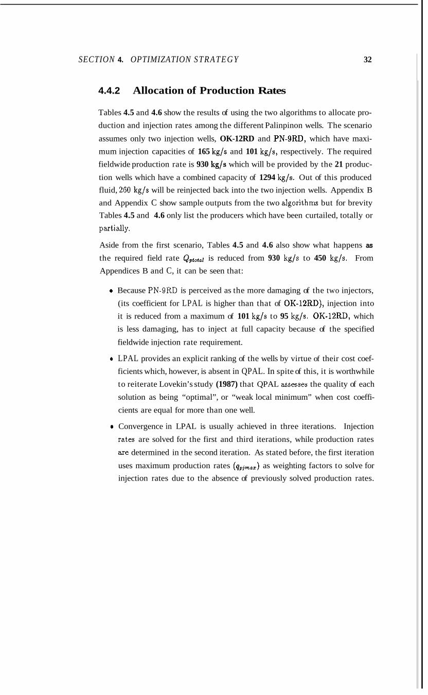
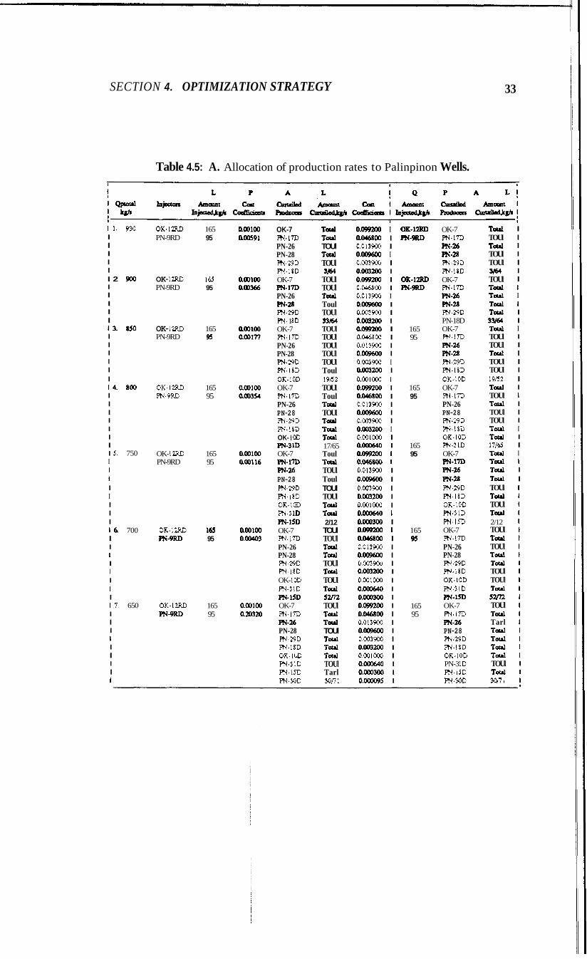
4.4.2 Allocation of Production Rates
Tables 4.5 and 4.6 show the results of using the two algorithms to allocate pro- duction and injection rates among the different Palinpinon wells. The scenario
assumes only two injection wells, OK-12RD and PN-9RD, which have maxi- mum injection capacities of 165 kg/s and 101 kg/s, respectively. The required fieldwide production rate is 930 kg/s which will be provided by the 21 produc-
tion wells which have a combined capacity of 1294 kg/s. Out of this produced fluid, 260 kg/s will be reinjected back into the two injection wells. Appendix B and Appendix C show sample outputs from the two algorithms but for brevity Tables 4.5 and 4.6 only list the producers which have been curtailed, totally or
partial1,y.
Aside from the first scenario, Tables 4.5 and 4.6 also show what happens as the required field rate Qptotal is reduced from 930 kg/s to 450 kg/s. From Appendices B and C, it can be seen that:
0 Because PN-9RD is perceived as the more damaging of the two injectors,
(its coefficient for LPAL is higher than that of OK-12RD)) injection into it is reduced from a maximum of 101 kg/s to 95 kg/s. OK-l2RD, which is less damaging, has to inject at full capacity because of the specified
fieldwide injection rate requirement.
0 LPAL provides an explicit ranking of the wells by virtue of their cost coef- ficients which, however, is absent in QPAL. In spite of this, it is worthwhile to reiterate Lovekin’s study (1987) that QPAL assesses the quality of each
solution as being “optimal”, or “weak local minimum” when cost coeffi-
cients are equal for more than one well.
0 Convergence in LPAL is usually achieved in three iterations. Injection
rat’es are solved for the first and third iterations, while production rates
arc: determined in the second iteration. As stated before, the first iteration
uses maximum production rates ( q p j m a z ) as weighting factors to solve for injection rates due to the absence of previously solved production rates.
SECTION 4. OPTIMIZATION STRATEGY 33
Table 4.5: A. Allocation of production rates to Palinpinon Wells.
11. 930 I I I I I I 2 900 I I I I I 13. 850 I I I I I I 14. 800 I I I I I I I I 5. 750 I I I I I I I I 16 700 I I I I I I 1 I 17. 650 I I I I I I I I 1
OK-1ZRD PN-9RD
OK- 12RD PN-9RD
OK- l2RD PN-9RD
OK-12RD PN-9RD
OK- 12RD PN-9RD
OK-12RD PN-9RD
OK-12RD m9m
165 95
I65 95
165 %
165 95
165 95
163 95
165 95
OK-7 PN- 17D PN-26 PN-28 PN-29D PN- 18D OK-7 P N - 1 7 D PN-26 PN-28 PN-29D PN- 1 8D OK-7
PN-26 PN-28 PN-29D PN-I8D OK-1OD OK-7
PN-26 PN-28 PN-29D
OK- 1m OK-7
PN-26 PN-28 PN-29D PN-18D OK-lOD
PN- 1sD OK-7 PN- 17D PN-26 PN-28 PN-29D PN- 18D OK- 1oD PN-31D PN- l!m OK-7 PN- 17D PN-26 PN-28 PN-29D PN- 18D OK-1CD PN-3 ID PN-15D PN-3OD
m-m
m-1m
m - 1 8 ~
m - 3 ~ m-1m
PN-3 ID
T d T d TOUl T d TOUl 3/64
TOUl TOUl TOUl Toul TOUl 33/64 TOUl TOUl TOUl TOUl TOUl Toul
TOUl Toul TOUl TOUl TOUl T d T d 17/65 Toul Tarl TOUl Toul TOUl TOUl T d T d 2/12 TOUl TOUl T d TOUl TOUl T d TOUl T d 52112 TOUl TOUl TOUl TOUl T d T d TOUl TOUl Tarl
19/52
3on1
0.0992oO I 0.046800 I 0.013900 I 0.009600 I 0.003900 I 0.003200 I 0.099Ux) I 0.046800 I 0.013900 I 0.009600 I o m 9 0 0 I 0.003200 I 0.0992oO I 0.046800 I 0.013900 I 0.009600 I 0.003900 I 0.003200 I 0.001Ooo 1 0.0992oo I 0.046800 I 0.013900 I 0.009600 I 0.003900 I 0.m200 I 0.001Ooo I 0.000640 I 0.0992oo 1 0.046800 1 0.013900 I 0.009600 I 0.003900 I 0.003Uw, I 0.001Ooo I 0.000640 1 0.ooom I 0.m200 1 0.046800 I 0.013900 I 0.009600 I 0.003900 I 0.003200 I 0.001Ooo I 0.000640 I 0.o0o300 I 0.0992oo I 0.046800 I 0.013900 I 0.009600 I 0.003900 I 0.003200 I 0.001oOo I 0.000640 I 0.ooom I 0.000095 I
OK-12RD PN-9RD
OK-17RD PN-9RD
165 95
165 95
165 95
165 95
165 95
OK-7 PN-17D PN-26 PN-28 PN-29D PN-18D OK-7 PN-17D PN-26 PN-28 PN-29D PN-18D OK-7 PN-17D PN-26 PN-28 PN-29D PN-18D OK-10D OK-7 PN-17D PN-26 PN-28 PN-29D PN-18D OK-1OD PN-31D OK-7
PN-26 PN-28 PN-29D PN-18D
m-m
OK-10D PN-31D PN-1sD OK-7 PN-17D PN-26 PN-28 PN-29D PN-18D OK-10D PN- ID pN-1sD OK-7 PN-17D
PN-28 PN-29D PN-18D OK-10D PN-3 1D PN-1SD PN-3OD
m-26
T 4 TOUl T d TOUl TOUl 3Ew TOUl T d Toul T d T d 33/64 TOUl TOUl TOUl T d TOUl TOUl
T d TOUl T d TOUl TOUl T d T d 17/65 T d T d T d T d TOUl T d TOUl T d 2/12 TOUl T d TOUl TOUl T d TOUl TOUl T d 52/32 TOUl T d Tarl T d T d T d T d TOUl T d 3W1
19/52
I I I I I I I 1 I 1 I I I I I I I I I I 1 I I I I I I I I I I
SECTION 4. OPTIMIZATION STRATEGY 34
Table 4.6: B. Allocation of production rates to Palinpinon Wells.
18. 600 I I I I I I I I I I I 9. 550 I I I I I I I I I 1 I 110. 500 I I I I I I I I I I I Ill . 450 I I I 1 I I I I I I I I
OK- l2RD PN-9RD
OK- 12RD PN-9RD
OK-1ZRD PN-9RD
OK- 12RD m - 9 ~ ~
I65 %
165 95
165 95
165 95
OK-7 m-m m-26 PN-28 PN-29D PN- 18D OK- 1oD PN-31D PN-1SD PN-3OD PN-16D OK-7 PN- 17D PN-26 PN-28 PN-29D PN- 18D OK- 1oD m - 3 1 ~ m- ~ S D PN-30D PN- 16D PN-23D OK-7
PN-26 PN-28 PN-29D PN-18D OK- 1oD
m-m
m - 3 1 ~ PN-ISD PN-30D PN-16D PN-23D OK-7 PN- 17D PN-26 PN-28 PN-29D PN-18D OK-1oD PN-3 1D PN- 1sD PN-30D PN- 16D PN-23D PN-19D
T d Tarl T d T d T d T d T d T d T d T d 9/46
T d T d T d T d T d T d T d Tarl T d T d Toul
TOUl T d Tarl TOUl T d T d T d Tarl TOUl T d T d
TOUl Tarl T d T d T d TOUl TOW T d T d Tarl T d T d NE4
13/13
63113
ox)99aDo I 0.046800 I 0.013900 I
0.003900 I 0.003200 I 0.001oOo I 0.000640 I 0.00M00 I 0.000095 I 0.000047 I 0.0992oo I 0.046800 I 0.013900 1 o.omsO0 I 0.003900 1 0.003200 I 0.M)loOo I 0.000640 1 0.000300 I 0.000095 I 0.000047 I 0.000055 I 0.0992w I 0.046800 I 0.013900 I
0.009600 I
165 95
165 95
165 95
OK-7 PN-17D lu-26 PN-28 PN-29D PN-18D OK-1OD PN-3 ID PN-1SD PN-30D PN-16D OK-7 PN-17D PN-26 PN-2.8 PN-29D PN-l8D OK-10D PN-31D
PN-m PN-16D PN-23D OK-7
PN-26
m-1m
T d T d T d T d T d T d T d T d T d T d 9/46 TOUl T d T d T d T d T d T d T d TOUl T d T d 1Un TOUl T d T d
I I I I I I I I I I I I I I I I I I I I I I I I I I
0.009600 0.003900
0.001oOo 0.000640 0.000300 0.000095
ammo
I I I I I I I
0.000047 1 0.000055 I 0.0992oO I 0.046800 I 0.013900 1 0.009600 I 0.mw I 0.003m I 0.001oOo 1 0.000640 I o.ooom I 0.000095 I 0.000047 I 0.000055 I O.ooOo14 I
165 95
PN-28 PN-29D PN-18D OK-10D PN31D PN-1SD PN-30D PN-16D PN.23D OK-7 PN-17D PN-26 PN-28 PN-29D PN-18D OK-10D PNJ1D PN-1SD PN-30D PN-16D PN-23D PN-19D
T d T d T d T d T d TOUl T d T d w3 T d T d T d T d TOUl T d T d T d TOUl T d TWl Tarl 44166
I I I I I I I I I I I I I I I
SECTION 4. OPTIMIZATION STRATEGY 35
The arc costs are solved, then summed up to find the cost coefficients for
the two injectors. After LPAL optimization, the injection rates are as- signed. For the second iteration, the injection rates determined from the first are included as weighting factors to obtain the arc costs, which are then summed to find the cost coefficients of the producing wells. Optimiza- tion follows and production rates are calculated. The third iteration then
uses these production rates as weighting factors and repeats the same pro-
cedure all over again to obtain the final injection rates. Since these rates are similar to those obtained from the first iteration, execution is halted;
otherwise, the cycle is resumed until convergence is achieved. When the
initial feasible solution identified in Phase I is also the optimal solution, the fieldwide breakthrough indices are identical for Phases I and 11.
0 Cycling in LPAL has not been observed during the numerous runs exe- cuted. Nevertheless, to prevent this from occurring, the input asks for the
maximum allowable number of iterations.
0 Production wells not shown in Tables 4.5 and 4.6 produce at maximum
capacity while production wells deemed to suffer thermal breakthrough
are ranked and shut-in accordingly. On the basis of the input data, the
program ranks OK-7, PN-l7D, PN-26, PN-28, PN-29D, and PN-18D as wells most vulnerable and, consequently, curtails them completely. As the required fieldwide production rate is reduced, Tables 4.5 and 4.6 show varying injection cost coefficients and throttling of the production wells
one by one. However, since ranking and allocation of the injectors are the same for all cases, the cost coefficients for the producers remain the same.
0 It can be concluded that QPAL and LPAL allocate the same rates to
injection and producing wells.

Section 5
Use of Chloride Data
The preceding section has shown that the algorithms using linear and quadratic
programming in conjunction with tracer data, field geometry and field operat-
ing conditions can be used to allocatk production and injection rates among the
different Palinpinon wells. With tracer tests, especially radioactive tracer tests,
it is possible to quantify the rate and extent of interaction between a producing and reinjecting well. Studies (LANL, 1987) have shown that by periodically injecting chemically reactive tracers for the appropriate temperature range and determining the extent of each reaction for each tracer in the production well,
the movement of thermal fronts in a reservoir can be tracked with time. How- ever, economic and operational constraints prohibit injecting tracers into each
reinjection well and monitoring all the production wells. Therefore, attention
was turned into finding other parameters that can be used in place of tracer data as input to the optimization routine. This parameter should be an arc-specific weighting factor manifesting a relationship between the injector and producer.
Preferably, it should be sensitive to changes in the utilization of either well and
at best, is independent of other injector and producer operating conditions.
One such parameter that has been inferred to show relationship between the injecting sector and the producing sector is the concentration of the chloride in
36
SECTION 5. USE OF CHLORIDE DATA 37
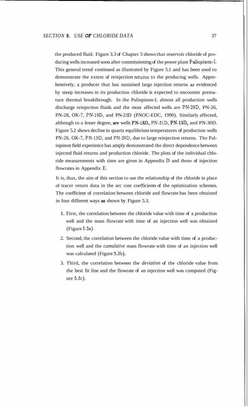
the produced fluid. Figure 3.3 of Chapter 3 shows that reservoir chloride of pro-
ducing wells increased soon after commissioning of the power plant Palinpinon-I. This general trend continued as illustrated by Figure 5.1 and has been used to demonstrate the extent of reinjection retu'rns to the producing wells. Appre- hensively, a producer that has sustained large injection returns as evidenced
by steep increases in its production chloride is expected to encounter prema- ture thermal breakthrough. In the Palinpinon-I, almost all production wells discharge reinjection fluids and the most affected wells are PN-29D, PN-26,
PN-28, OK-7, PN-19D, and PN-23D (PNOC-EDC, 1990). Similarly affected,
although to a lesser degree, are wells PN-l8D, PN-31D, PN-l5D, and PN-30D.
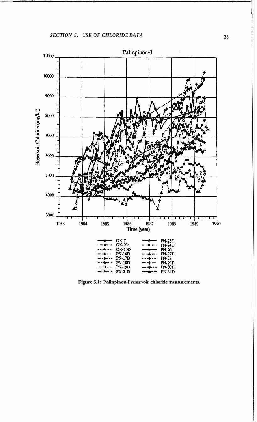
Figure 5.2 shows decline in quartz equilibrium temperatures of production wells PN-26, OK-7, PN-19D, and PN-29D, due to large reinjection returns. The Pal- inpinon field experience has amply demonstrated the direct dependence between
injected fluid returns and production chloride. The plots of the individual chlo-
ride measurements with time are given in Appendix D and those of injection flowrates in Appendix E.
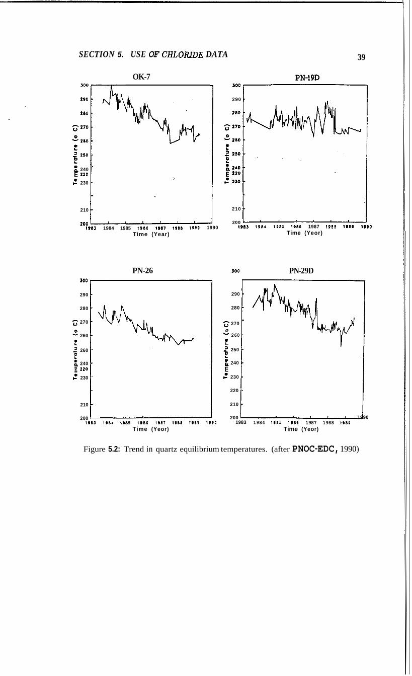
It is, thus, the aim of this section to use the relationship of the chloride in place of tracer return data in the arc cost coefficients of the optimization schemes. The coefficient of correlation between chloride and flowrate has been obtained
in four different ways as shown by Figure 5.3.
1. First, the correlation between the chloride value with time of a production well and the mass flowrate with time of an injection well was obtained
(Figure 5.3a).
2. Second, the correlation between the chloride value with time of a produc-
tion well and the cumulative mass flowrate with time of an injection well was calculated (Figure 5.3b).
3. Third, the correlation between the deviation of the chloride value from the best fit line and the flowrate of an injection well was computed (Fig-
ure 5 .3~) .
SECTION 5. USE OF CHLORIDE DATA 38
1983 1984 1985 1986 1987 Time (year)
1988 1989
PN-UD PN-24D PN-26 PN-27D PN-28 PN-29D PN-30D PN-31D
Figure 5.1: Palinpinon-I reservoir chloride measurements.
SECTION 5. USE OF CHLORJDE DATA 39
OK-7
f 2 2so - E : 240 E
- : 230 -
210
220 i 1984 1985 lS86 1S87 1988
Time (Year) lS89
-
1990
PN-26
290
280
270 - 260 0
2 1 260 f
E 240 ’
c” 230
220 i 210
200 I t
1983 1984 lS8S 1986 1987 lS88 lS89 1990 Time (Yeor)
I PN- 19D
290 1
210
220 i 200 I I I
1983 1984 lB85 lS86 1987 1918 Time (Yeor)
1989
PN-29D m 0 I 290 - 280 -
I; 270 - 260 - e
2 250 -
- 0
L
E E
240 - t” 230 -
220 - 210 - 200 1 I
I I
1983 1984 1985 lB86 1987 1988 Time (Yeor)
~
19B9 I 1990
Figure 5.2: Trend in quartz equilibrium temperatures. (after PNOC-EDC, 1990)
SECTION 5. USE OF CHLORIDE DATA 40
Time
Time Figure 5.3a Chloride vs flowrate
Time
Figure 5.3b Chloride vs Cumulative flow
I Time
Qure 53c Chloride deviation vs Flowrate
Figure 5.3: Chloride vs fiowrate correlation methods.
SECTION 5. USE OF CHLORIDE DATA 41
4. Lastly, the chloride value with time of a production well was expressed as a linear combination of the mass flowrates of the injection wells.
The two radioactive tracer tests (PN-9RD and OK-12RD) which show conclu-
sively which reinjection well interacts with which production wells were used to
test the applicability of the correlation method.
5.1 ChlorideFlowrate Correlation Method
By visual inspection of a figure similar to Figure 3.3, it has been observed that certain production wells react strongly to particular injection wells. If an injection well communicates intensely with a production well, then putting
this injection well on line is usually followed by a substantial increase in the
chloride measurements of the affected well. Once it is removed from service, there is an accompanying decrease in the chloride data of the producing well. It
is assumed, then, that there is a linear relationship between the flowrate of an injection well, (q,.;), and the magnitude of the chloride value of a producing well, (d;). To obtain a measure of the strength of the linear relationship between these two variables, the coefficient of correlation r , independent of the respective scales of measurement, was calculated according to the formula:
where n is the number of data points, and:
n
SECTION 5. USE OF CHLORIDE DATA 42
5.1.1 PN-9RD Tracer Test Application
Figure 51.4 shows the injection flowrates of injection well PN-9RD and the chlo-
ride values of production well OK-7. It can be recalled that the PN-9RD tracer
test has shown immediate and large returns to OK-7 of the tracer injected into PN-9RD.
Figure 5.4 demonstrates the general trend of increasing chloride values of OK- 7. The plot, however, is characterized by periods of steep ups and down in the
chloride values. As an example, peaks occurred during the times June 1984,
October 1985, and July 1986. On the other hand, PN-9RD was utilized only for two intervals of time: from April-July, 1984, and February-October, 1985.
By looking at the graphs, one notes that the peak of PN-9RD use on July 1984
(40 kg/tj) coincides exactly with the chloride peak of OK-7. Putting PN-9RD on service on April 1984 was followed immediately by large increases in OK-7 chloride values. However, if this increase in OK-7 chloride is attributed only to PN-9RD, the absence of the peaks and dips corresponding to the May-July use
of PN-SRD, during which the monthly average injection flowrate of PN-9RD increased to 40 kg/s, down to 17 kg/s, and up again to 40 kg/s, would cast a doubt 0x1 the method. This can be explained by the fact that some precision on
results had been sacrificed with the use of monthly averages. By plotting the raw
data of OK-7 chloride with PN-9RD flowrate (Figure 5.5)) the accompanying and expected effect on OK-7 for this interval is more evident. Nevertheless,
the rest of the report shall continue to use monthly average chloride values for
consistency with that of the injection flowrates. It is believed that in spite of
this, the loss of finer details is not significant enough to alter the conclusions that have been reached.
For the second time interval (February-October, 1985) when PN-9RD was in- jecting in greater quantities (80 kg/s), there is also a corresponding increase and
decrease in OK-7 chloride. It is interesting to observe that the start of the steep
increase in OK-7 chloride (March 1985) coincides with a similar increase in in-
jection into PN-9RD (from 5 to 71 kg/s). The peak, however, of OK-7 chloride
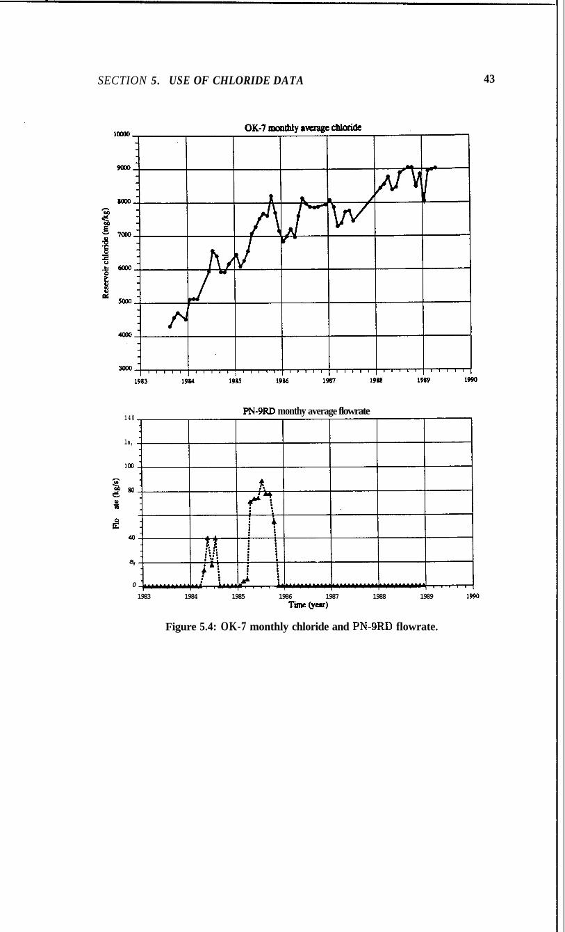
SECTION 5. USE OF CHLORIDE DATA 43
PN-9RD monthy average flowrate 1 4 0
la,
100
h 380 3 3
40
a,
0
1983 1984 1985 1986 1987 1988 1989 1990 Ti= olep)
Figure 5.4: OK-7 monthly chloride and PN-9RD flowrate.
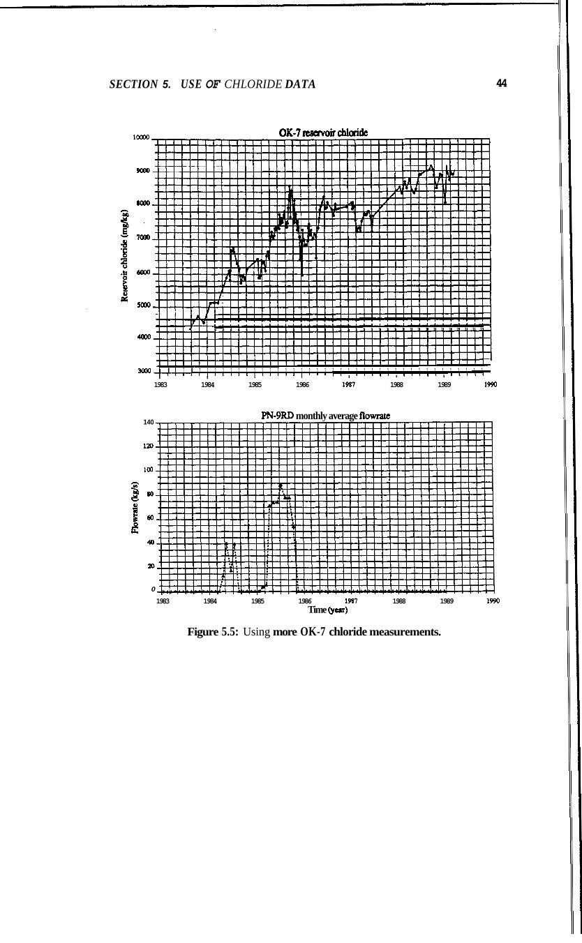
SECTION 5. USE OF CHLORIDE DATA 44
loo00
9OOo
1 1 1 1 1 1 1 1 l 1 1 1 1 1 1 1 1 1 1 1 1 1 1 1 1 1 1 1 1 1 1 1 1 1 1 1 1 1 I I I I I
I I I I I I I I I I I I ~ I I ~ I I I I I I I I I I I I I I I I I I I 1 1 1 1 1 1 1 1 1 1 1 1 1 1 1 1 1 1 1 1 1 1 1 1 1 1 1 1 1 1 1 1 1 1 1
I I I I I I I I I I I I I I I I I I I I I I I I I I I I I I I I I I I I I I I I I I 3Ooo I I I I I I 1 1 1 1 1 1 1 1 1 1 1 1 1 1 1 1 1 1 1 1 1 1 1 1 1 1 1 1 1 1 1 1 1 1 1 1
1 1 I I I I I I I I I I I I l I l
1983 1984 1985 1986 1987 1988 1989 1990
140 PN-9RD monthly average flowme
120
100
n 380 h a Q
40
m
0
1983 1984 1985 1986 1987 1988 1989 1990 Time &ea)
Figure 5.5: Using more OK-7 chloride measurements.
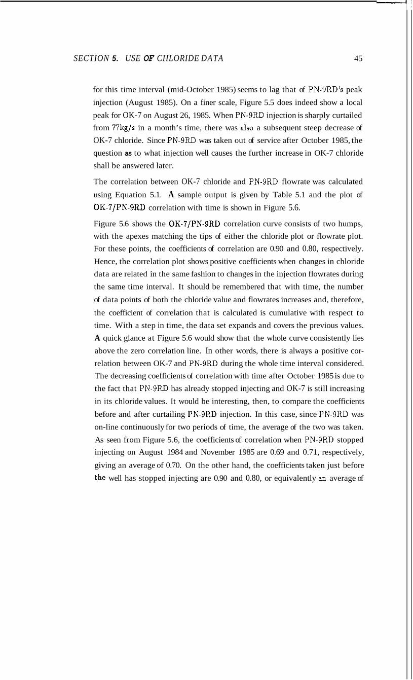
SECTION 5. USE OF CHLORIDE DATA 45
for this time interval (mid-October 1985) seems to lag that of PN-9RD’s peak
injection (August 1985). On a finer scale, Figure 5.5 does indeed show a local
peak for OK-7 on August 26, 1985. When PN-9RD injection is sharply curtailed from 77kg/s in a month’s time, there was .also a subsequent steep decrease of OK-7 chloride. Since PN-9RD was taken out of service after October 1985, the question as to what injection well causes the further increase in OK-7 chloride shall be answered later.
The correlation between OK-7 chloride and PN-9RD flowrate was calculated
using Equation 5.1. A sample output is given by Table 5.1 and the plot of
OK-7/PN-SRD correlation with time is shown in Figure 5.6.
Figure 5.6 shows the OK-7/PN-9RD correlation curve consists of two humps, with the apexes matching the tips of either the chloride plot or flowrate plot. For these points, the coefficients of correlation are 0.90 and 0.80, respectively.
Hence, the correlation plot shows positive coefficients when changes in chloride data are related in the same fashion to changes in the injection flowrates during
the same time interval. It should be remembered that with time, the number
of data points of both the chloride value and flowrates increases and, therefore,
the coefficient of correlation that is calculated is cumulative with respect to time. With a step in time, the data set expands and covers the previous values. A quick glance at Figure 5.6 would show that the whole curve consistently lies
above the zero correlation line. In other words, there is always a positive cor- relation between OK-7 and PN-9RD during the whole time interval considered. The decreasing coefficients of correlation with time after October 1985 is due to the fact that PN-9RD has already stopped injecting and OK-7 is still increasing
in its chloride values. It would be interesting, then, to compare the coefficients
before and after curtailing PN-9RD injection. In this case, since PN-9RD was
on-line continuously for two periods of time, the average of the two was taken.
As seen from Figure 5.6, the coefficients of correlation when PN-9RD stopped injecting on August 1984 and November 1985 are 0.69 and 0.71, respectively,
giving an average of 0.70. On the other hand, the coefficients taken just before
the well has stopped injecting are 0.90 and 0.80, or equivalently an average of
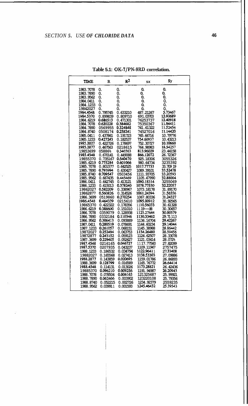
SECTION 5. USE OF CHLORIDE DATA 46
Table 5.1: OK-?/PN-SRD correlation.
TIME R R2 sx SY
1983.7078 0. 0. 1983.7890 0. 0. 1983.9562 0. 0. 1984.0411 0. 0. 1984.1233 0. 0. 19842027 0. 0. 1984.4548 0.795745 0.633210 19845370 0.899839 0.809710 1984.6219 0.6$6513 0.471301 1984.7078 0.620228 0.384682 1984.7890 0569955 0.324848 1984.8740 0508174 0258241 1985.041 1 0.437861 0.191723 1985.1233 0.4272A3 0.182537 19852027 0.422726 0.178697 19852877 0.467563 0218615 19853699 05886% 0.346563 1985.4548 0.670141 0.449088 19855370 0.735167 0540470 1985.6219 0.775284 0.601066 1985.7078 0.801577 0.642525 1985.7890 0.793994 0.630427 1985.8740 0.709547 0503456 1985.9562 0.667435 0.445469 1986.0411 0.642745 0.413121 1986.1233 0.615013 0378240 19862027 0582209 0.338967 19862877 0560826 0.314526 1986.3699 0519860 0270254 1986.4548 0.464339 0215610 19865370 0.422322 0.178356 1986.6219 0.388600 0.151010 1986.7078 0359079 0.128938 1986.7890 0332184 0.110346 1986.9562 0306413 0.093889 1987.0411 030519 0.078691 1987.1233 0261057 0.068151 19872027 0252494 0.063753 19872877 0243152 0.059123 1987.3699 0229405 0.052627 1987.4548 0216165 0.046727 19875370 0207935 0.043237 1988.1233 0.186532 0.034794 19882027 0.165568 0.027413 19882877 0.143859 0.020695 1988.3699 0.128799 0.016589 1988.4548 0.114131 0.013026 19885370 0.096210 0.009256 1988.7078 0.078504 0.006163 1988.7890 0.062466 0.003902 1988.8740 0.052215 0.002726 1988.9562 0.03991 1 0.001593
0. 0. 0. 0. 0. 0.
487.21267 69 1.03703 76253737 75350367 741.61322 74527016 765.66716 754.60937 752.30727 764.98983 813.96029 866.12072 925.18306 980.64734
1089.39101 1111.93705 1105.47990 1090.18314 1078.77530 1073.18178 1061.24394 1067.80336 1095.00912 11 1056033 11 19-38 112527644 1130.33462 1136.16704 1144.60234 1145.38988 113426480 1124.62507 1121.03414 11 17.77560 1109.11947 1122.9641 1 113853303 1159.01786 1165.76772 117328821 1191.94987 121325687 123220108 1234.92379 1245.46432
1017.7n33
0. 0. 0. 0. 0. 0. 5.73467 12.92689 12.40918 11.94411 1152454 11.14420 10.79776 10.43213 10.10660 1854257 23.44158 26.72367 3055326 3235392 33.709 19 3352478 3320593 32.88004 3255069 32.22057 31.89170 3 156556 3 1.24327 30.92565 30.61328 30.30657 30.00579 29.71 113 29.42267 29.14044 28.86442 2859456 28.33078 28.072% 27.82099 2757475 27 33408 27.09886 26.86893 26.64414 26.42436 2620943 25.99921 25.79356 2559235 25.39543
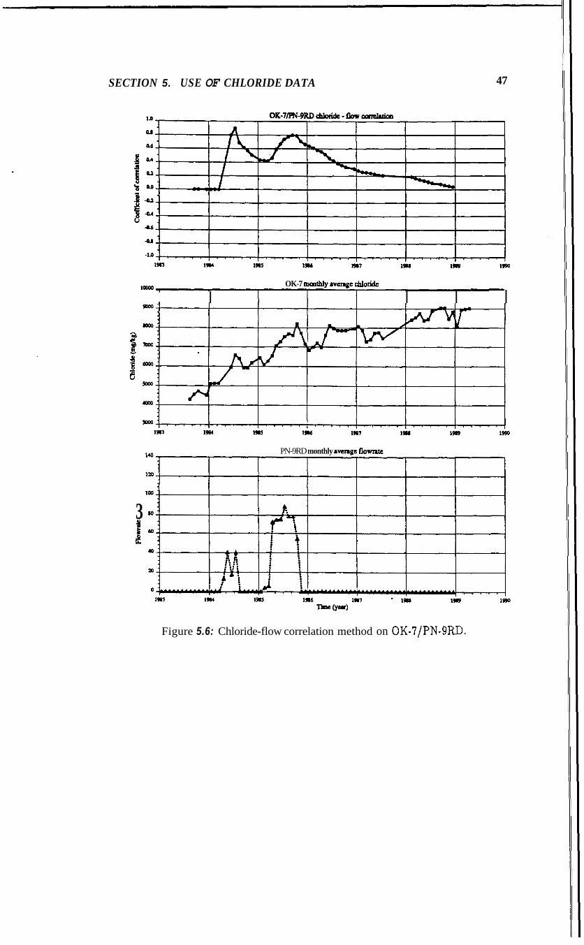
SECTION 5. USE OF CHLORIDE DATA 47
lam OK-7 m d d y avenge chloride
I I I I
140 PN-9RD monthly avemge flowrue
no i
3
Figure 5.6: Chloride-flow correlation method on OK-'I/PN-SRD.
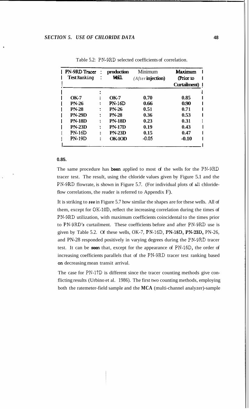
SECTION 5. USE OF CHLORIDE DATA 48
Table 5.2: PN-9RD selected coefficients of correlation.
I PN-9RDTraccr : production Minimum Maximum I I Test Ranking : Well ( A f t e r injection) (Priorto I ! Curtailment) I
I OK-7 : OK-7 0.70 0.85 I I PN-26 : PN-16D 0.66 0.90 I I PN-28 : PN-26 0.5 1 0.7 1 I I PN-29D : PN-28 0.36 0.53 I I PN-18D : PN-18D 0.23 0.3 1 1 I PN-23D : PN-17D 0.19 0.43 I I PN-16D : PN-23D 0.15 0.47 I I PN-19D : OK-1OD -0.05 -0.10 I I I
0.85.
The same procedure has been applied to most of the wells for the PN-9RD tracer test. The result, using the chloride values given by Figure 5.1 and the
PN-9RD flowrate, is shown in Figure 5.7. (For individual plots of all chloride- flow correlations, the reader is referred to Appendix F).
It is striking to see in Figure 5.7 how similar the shapes are for these wells. All of
them, except for OK-lOD, reflect the increasing correlation during the times of PN-9RD utilization, with maximum coefficients coincidental to the times prior to PN-9RD’s curtailment. These coefficients before and after PN-9RD use is given by Table 5.2. Of these wells, OK-7, PN-16D, PN-l8D, PN-23D, PN-26, and PN-28 responded positively in varying degrees during the PN-9RD tracer
test. It can be seen that, except for the appearance of PN-16D, the order of
increasing coefficients parallels that of the PN-9RD tracer test ranking based on decreasing mean transit arrival.
The case for PN-17D is different since the tracer counting methods give con- flicting results (Urbino et al. 1986). The first two counting methods, employing
both the ratemeter-field sample and the MCA (multi-channel analyzer)-sample
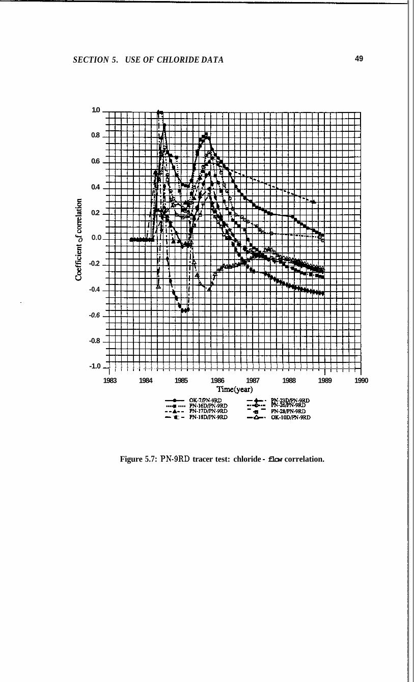
SECTION 5. USE OF CHLORIDE DATA 49
rw 0
1.0
0.8
0.6
0.4
0.2
0.0
-0.2
-0.4
-0.6
-0.8
-1.0 1 1 1 1 1 1 1 1 1 1 1 1 1 1 1 1 1 1 1 1 1 1 1 1 1 1 1 1 1 1 1 1 1 1 1 1 1 1 1 1 1 1
1983 1984 1985 1986 1987 1988 1989 1990 Time(year)
+ OK-7IPN-9RD - - PN-23DPN9RD
--A- - PN-I’IDPNBRD - II - PN-am-9RD - t - PN-lSDPN-9RD -&* OK-lODIpN-9RD
.... .... ~ ~ - 1 m p 1 q - 9 ~ ~ -*+*I PN-26PN-9RD
Figure 5.7: PN-9RD tracer test: chloride - flow correlation.
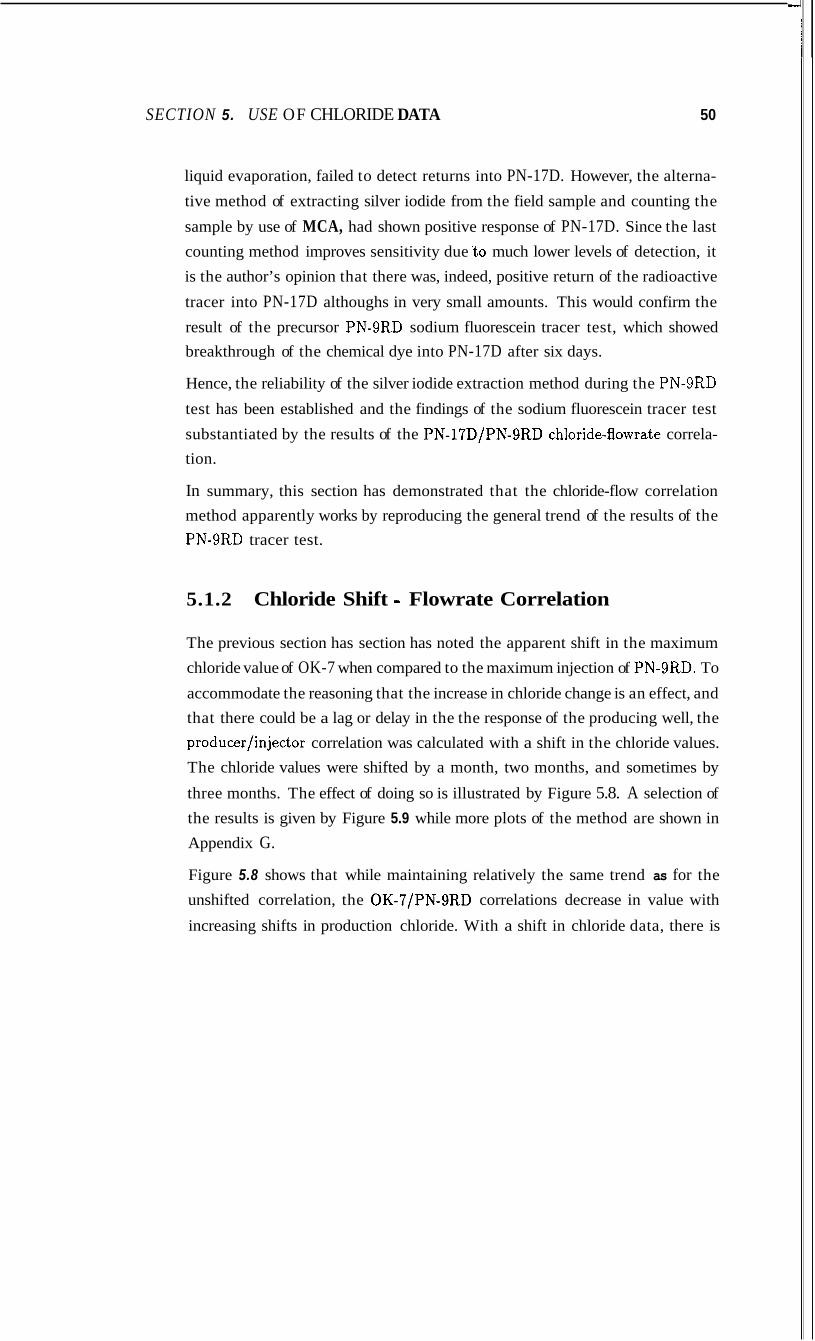
SECTION 5. USE OF CHLORIDE DATA 50
liquid evaporation, failed to detect returns into PN-17D. However, the alterna-
tive method of extracting silver iodide from the field sample and counting the
sample by use of MCA, had shown positive response of PN-17D. Since the last counting method improves sensitivity due 10 much lower levels of detection, it is the author’s opinion that there was, indeed, positive return of the radioactive
tracer into PN-17D althoughs in very small amounts. This would confirm the
result of the precursor PN-9RD sodium fluorescein tracer test, which showed breakthrough of the chemical dye into PN-17D after six days.
Hence, the reliability of the silver iodide extraction method during the PN-9RD test has been established and the findings of the sodium fluorescein tracer test
substantiated by the results of the PN-17D/PN-SRD chloride-flowrate correla- tion.
In summary, this section has demonstrated that the chloride-flow correlation method apparently works by reproducing the general trend of the results of the PN-9RD tracer test.
5.1.2 Chloride Shift - Flowrate Correlation
The previous section has section has noted the apparent shift in the maximum chloride value of OK-7 when compared to the maximum injection of PN-9RD. To
accommodate the reasoning that the increase in chloride change is an effect, and that there could be a lag or delay in the the response of the producing well, the producer/injector correlation was calculated with a shift in the chloride values. The chloride values were shifted by a month, two months, and sometimes by
three months. The effect of doing so is illustrated by Figure 5.8. A selection of
the results is given by Figure 5.9 while more plots of the method are shown in Appendix G.
Figure 5.8 shows that while maintaining relatively the same trend as for the unshifted correlation, the OK-7/PN-9RD correlations decrease in value with
increasing shifts in production chloride. With a shift in chloride data, there is
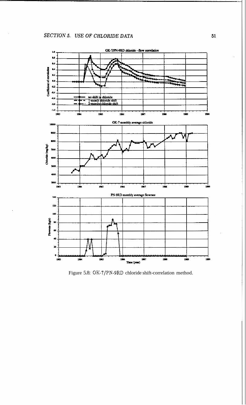
Figure 5.8: OK-'I/PN-SRD chloride shift-correlation method.
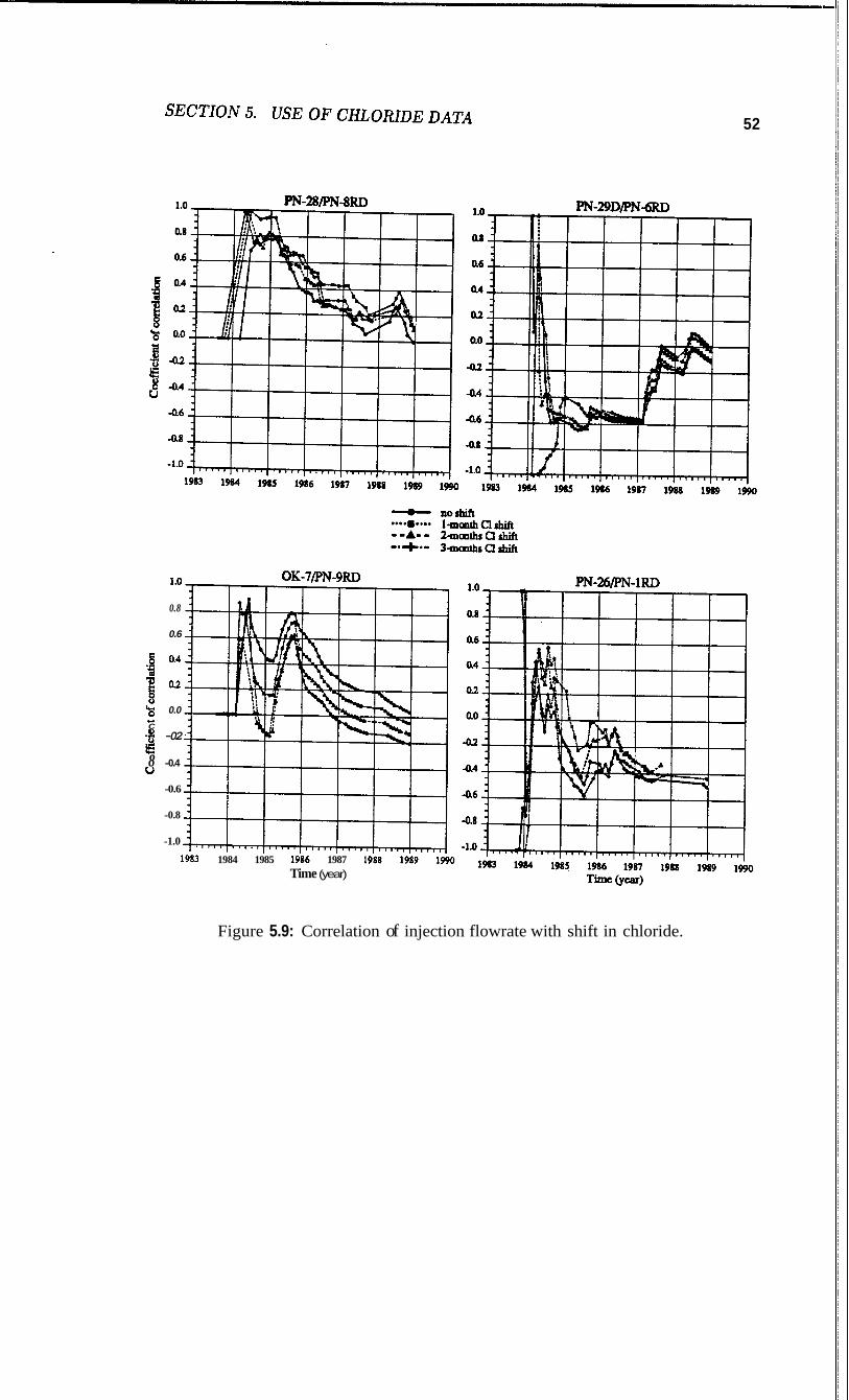
I .o
0.8
0.6
0.4
OK-7PN-9RD
-1 0.2 ‘i; 0.0
-9 -02
8 -0.4
- C
a U
-0.6
-0.8
-1.0
1983 1984 1985 1986 1987 I988 lks9 1&1 Time (year)
52
Figure 5.9: Correlation of injection flowrate with shift in chloride.
SECTION 5. USE OF CHLORIDE DATA 53
also a shift in the maximum coefficients for the second hump or wave. Hence,
while the maximum was 0.80 on September 1985 for the unshifted correlation,
these were reduced to 0.73 on October 1985 for a one-month chloride shift.
However, a. two-month or three-month shift in chloride value does not shift the maximum by the same degree as the one-month shift. Hence, a two-month shift
has a maximum of 0.63 on October 1985, and a three-month chloride shift has
a maximum of 0.60 also on the same month.
This is the general trend for most of the chloride shifts as can be seen from the figures in Appendix G. However, there are some exceptions to this trend. Cor-
relations of OK-7 with injection wells PN-lRD, PN-2RD, and PN-SRD, for the
most part, are greater with shifts in chloride of OK-7. While the usual increase in the coefficients of 0.2 may not be sufficient to alter the prevailing correla- tion, sometimes the effect would be significant to do otherwise. As an example, correlations of OK-7 with PN-1RD and PN-2RD increase tremendously from
negative correlations to high positive correlations in the first fifth of the curve. Such is the case, too, for the PN-26/PN-lRD and PN-28/PN-lRD correlations.
Since the correlation trends with chloride shift do not significantly depart from
that with no shift, it would suffice to simply use the coefficients of correlation for no chloride shift.
5.1.3 OK012RD/PN-6RD Tracer Test Application
Figure 5.10 shows the injection flowrates of wells PN-6RD and the increases in
the reservoir chloride of well PN-17D. Figure 5.11 includes the result of finding
the correlation between the chloride data of PN-17D and the injection flowrates
of PN-6RD.
Due to the unavailability of data on injection well OK-l2RD, PN-6RD was used in its place on the basis of the sodium fluorescein test on OK-12RD which exhibited the unequivocal return of the dye on PN-6RD. (see Table 3.1). The
premise, then, is that a well which interacts with OK-12RD would interact with
SECTION 5. USE OF CHLORIDE DATA 54
PN-6RD due to the strong communication between the two.
FromFigure 5.10, it can be gleamed that PN-6RD was injecting for four intervals
of time: from Sept 1983-May 1984, from Nov 1984-Jan 1985, from Mar-Aug 1987 and from Apr- 1988. There are also two other brief periods which are Sept 1985 and Dec 1987. An inspection of the injection flowrates from Appendix E would
show that for the latter periods of PN-6RD injection, only PN-1RD injection
comes close to the PN-6RD plot. However, in both instances the start and end of injection into PN-6RD occurs before that of PN-1RD (e.g. Mar-Aug 1987 for PN-6RD as oppose to Jun-Nov 1987 for PN-1RD). There was also PN-8RD which was injecting from Oct 1987 - Aug 1988. It is important to recognize these differences in order to distinguish the effect of one injection well from that of another.
Figure 5.10 shows how similar the chloride and flowrate curves are for the first interval. The start of ascent, the decline, and the peaks coincide. This could be
interpreted as signifying a strong degree of correlation between PN-17D and PN- 6RD. For the second interval, the chloride values of PN-17D start to increase and decrease earlier than the hook-up of PN-GRD, hence it can be surmised that for this period other injection wells are contributing. It is, nevertheless, striking that in the brief period of Sept 1985, when PN-6RD comes on line
again after eight months, the chloride values of PN-17D start to increase at the
same time. However, the lack of PN-17D chloride measurements after October 1985, precludes further analysis between the two wells and necessitates other production wells, instead.
Figure 5.11 shows the chloride-flow correlation between PN-17D and PN-6RD. As discussed in the preceding paragraph, a high degree of correlation between
the two wells is indicated especially in the first interval of injection. For this interval, the coefficients range from 0.58 to 0.85 where 0.63 is the coefficient
prior to curtailment of PN-6RD and 0.58 after curtailment. This first interval
is followed by declining coefficients because of the increasing chloride values
simultaneous with the absence of injection into PN-GRD, as well as the lack of
SECTION 5. USE OF CHLORIDE DATA 55
140 PN-6RD monthy average flowrate
120
100
n a80 B t a t2
49
m
0
1983 1984 1985 1986 1981 1988 1989 1990 T i (year)
Figure 5.10: PN-17D chloride values and PN-6RD flowrate.
SECTION 5. USE OF CHL0R.DE DATA 56
Figure 5.11: Chlorideflow correlation method on PN-l'IDIPN-GRD.
!I I
SECTION 5. USE OF CHLORIDE DATA - 57
further measurements on PN-17D in the latter period.
The correlation of PN-6RD with other production wells monitored during the
OK-12RD tracer test was calculated, and the results are plotted in Figure 5.12. As listed in Table 3.1, the wells which responded positively during the OK-12RD tracer test are PN-l7D, OK-lOD, OK-7, PN-28, and PN-15D ranked according to percentage of tracer return. Traces were also found in PN-21D and PN-26.
Some points are worth noting in Figure 5.12 if the diagram is visualized as being
divided into strips corresponding to the intervals when PN-6RD is injecting (Sep
83-May 84, Nov 84-Jan 85, Mar-Aug 87, and Apr-Jul 88).
0 First, the high coefficients of correlation (0.46-0.99) are evident in the first interval corresponding to PN-6RD injection. A comparison between the
ranking provided by the OK-12RD tracer test and the selected coefficients in this first interval is provided by Table 5.3. This table shows a high degree
of correlation of PN-6RD with PN-28, OK-lOD, OK-7, PN-26, PN-l7D,
PN-l5D, and PN-21D on the basis of the maximum value of coefficients coincident with maximum injection into PN-6RD during this period. If the
criterion has been based on the correlation after PN-6RD injection, then the ranking would be shifted to PN-17D, PN-l5D, PN-28, PN-26, OK-7, and OK-1OD. Although the method does not provide an exact duplicate of
the tracer test ranking, it affirms the strong communication between these
pair of wells.
0 Second, most of the correlations decrease because PN-6RD was cut-off from the line. It can also be attributed to the scarcity of chloride measurements on the producing well during certain time intervals. Nevertheless, from Figure 5.12, it is very striking to see that in the next three intervals of time (Nov 84-Jan 85, Mar-Aug 87, and Apr-Jul 88) during which PN-6RD was injecting, the correlations of OK-7, PN-28, and PN-26 register a dramatic
change in their trends and correlations start increasing. The start and end
of these gradients correspond exactly with the onset and termination of
PN-6RD injection. Even the effect of the brief injection on Sept 1985 was
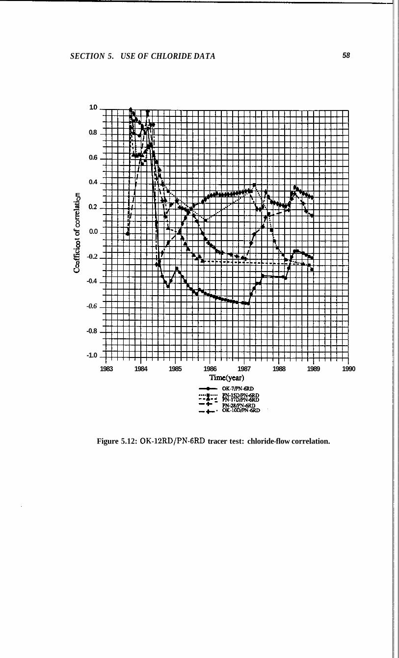
SECTION 5. USE OF CHLORIDE DATA 58
1 .o
0.8
0.6
0.4
! o-2
E 0
8 "0 0.0
8 g -0.2 8
Y
.- 0
u -0.4
-0.6
-0.8
-1.0
1983 1984 1985 1986 1987 1988 1989 1990 Time(year)
OK-'I/PNQU) e+....... pN-lm/PNQU) --A- - PN-17DPN6RD -t - PN-28/PNdRD 0 + OK-10DIpNa '
Figure 5.12: OK-12RD/PN-GRD tracer test: chloride-flow correlation.
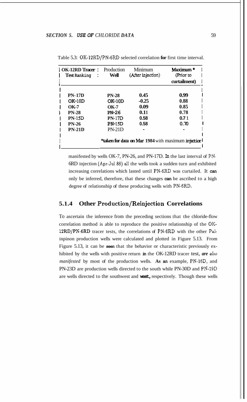
SECTION 5. USE OF CHLORIDE DATA 59
Table 5.3: OK-12RDIPN-GRD selected correlation for first time interval.
I OK-12RD Tracer : Production Minimum Maximum* I I Test Ranking : Well (Afterinjection) (priorto I I curtailment) I
I I 1 I
I I I 1 I I I I I 1
PN- 17D OK- 1OD OK-7 PN-28 PN- 15D PN-26 PN-21D
PN-28 0.45 0.99 OK- 1OD -0.25 0.88 OK-7 0.09 0.85 PN-26 0.1 1 0.78 PN- 17D 0.58 0.7 1 PN- 15D 0.58 0.70 PN-21D - -
*taken for data on Mar 1984 with maximum injectior
I I I I I I I I I 1
manifested by wells OK-7, PN-26, and PN-17D. In the last interval of PN- 6RD injection (Apr-Jul88) d l the wells took a sudden turn and exhibited increasing correlations which lasted until PN-6RD was curtailed. It can only be inferred, therefore, that these changes can be ascribed to a high
degree of relationship of these producing wells with PN-6RD.
5.1.4 Other Production/Reinjection Correlations
To ascertain the inference from the preceding sections that the chloride-flow
correlation method is able to reproduce the positive relationship of the OK- 12RD/PN-GRD tracer tests, the correlations of PN-6RD with the other Pal- inpinon production wells were calculated and plotted in Figure 5.13. From Figure 5.13, it can be seen that the behavior or characteristic previously ex-
hibited by the wells with positive return in the OK-12RD tracer test, are also manifested by most of the production wells. As an example, PN-16D, and
PN-23D are production wells directed to the south while PN-30D and PN-19D are wells directed to the southwest and west, respectively. Though these wells
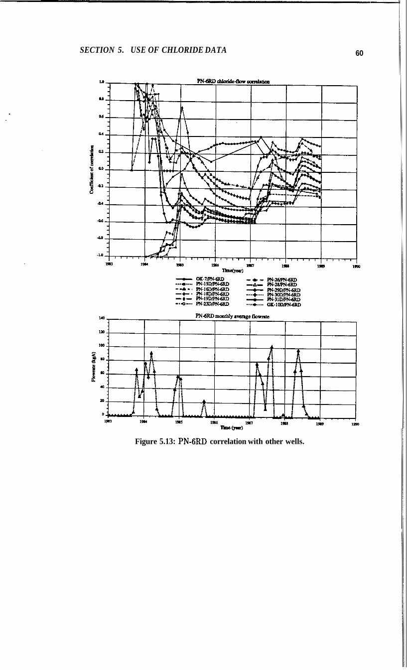
SECTION 5. USE OF CHLORIDE DATA 60
Figure 5.13: PN-6RD correlation with other wells.
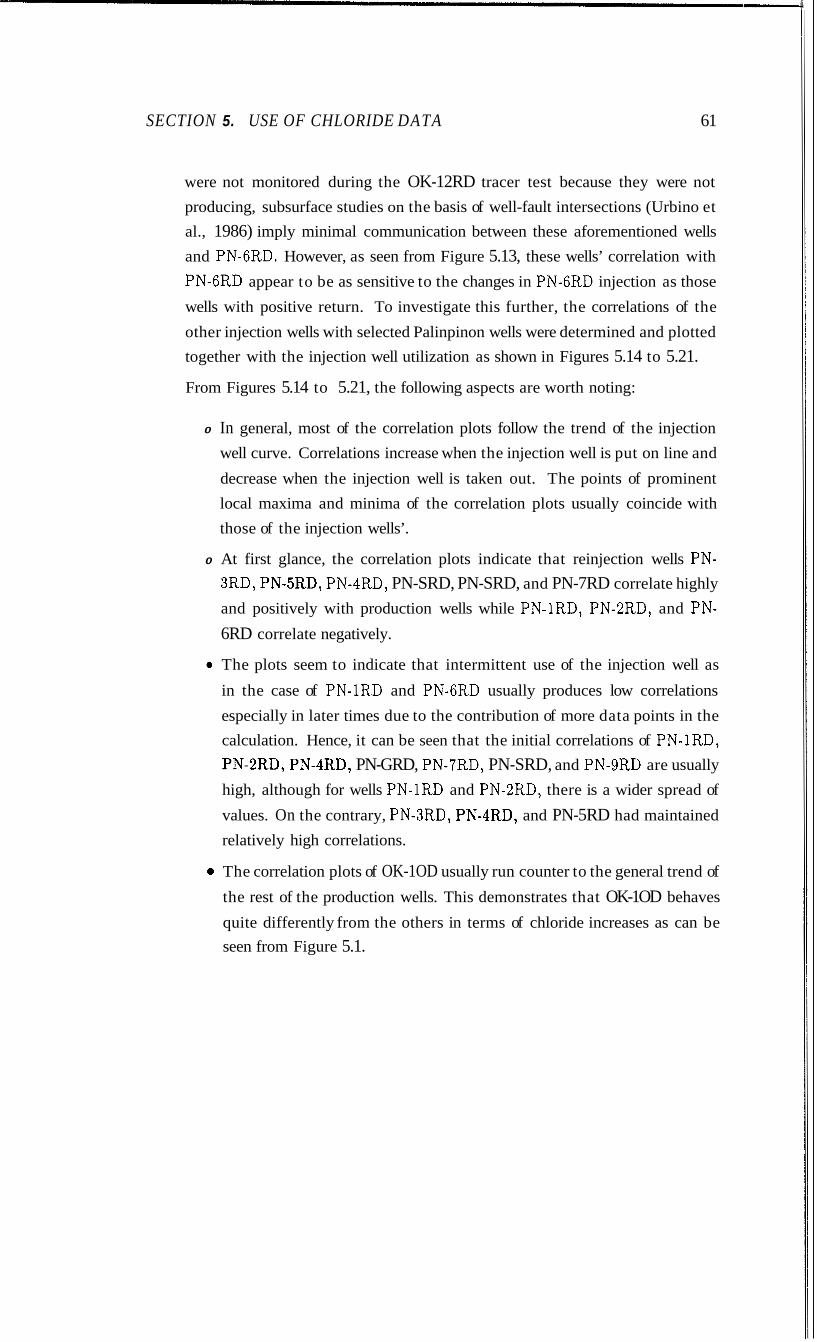
SECTION 5. USE OF CHLORIDE DATA 61
were not monitored during the OK-12RD tracer test because they were not producing, subsurface studies on the basis of well-fault intersections (Urbino et al., 1986) imply minimal communication between these aforementioned wells and PN-6RD. However, as seen from Figure 5.13, these wells’ correlation with
PN-6RD appear to be as sensitive to the changes in PN-6RD injection as those
wells with positive return. To investigate this further, the correlations of the
other injection wells with selected Palinpinon wells were determined and plotted together with the injection well utilization as shown in Figures 5.14 to 5.21.
From Figures 5.14 to 5.21, the following aspects are worth noting:
0 In general, most of the correlation plots follow the trend of the injection well curve. Correlations increase when the injection well is put on line and
decrease when the injection well is taken out. The points of prominent local maxima and minima of the correlation plots usually coincide with those of the injection wells’.
0 At first glance, the correlation plots indicate that reinjection wells PN- 3RD, PN-5RD, PN-4RD, PN-SRD, PN-SRD, and PN-7RD correlate highly and positively with production wells while PN-lRD, PN-2RD, and PN- 6RD correlate negatively.
0 The plots seem to indicate that intermittent use of the injection well as
in the case of PN-1RD and PN-6RD usually produces low correlations
especially in later times due to the contribution of more data points in the calculation. Hence, it can be seen that the initial correlations of PN-lRD, PN-2RD, PN-4RD, PN-GRD, PN-’IRD, PN-SRD, and PN-9RD are usually high, although for wells PN-1RD and PN-2RD, there is a wider spread of
values. On the contrary, PN-3RD, PN-4RD, and PN-5RD had maintained relatively high correlations.
0 The correlation plots of OK-1OD usually run counter to the general trend of
the rest of the production wells. This demonstrates that OK-1OD behaves
quite differently from the others in terms of chloride increases as can be seen from Figure 5.1.
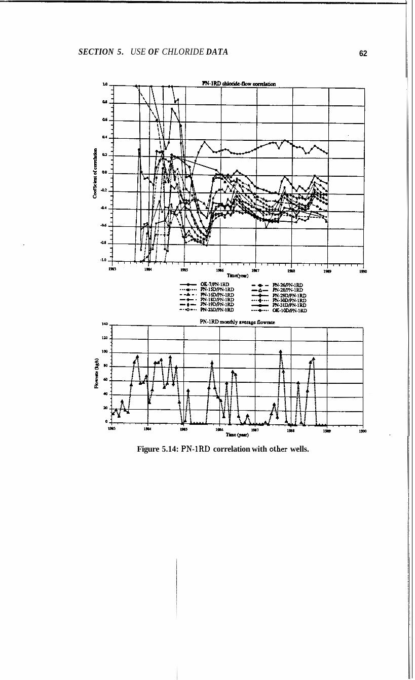
SECTION 5. USE OF CHLORIDE DATA 62
Figure 5.14: PN-1RD correlation with other wells.
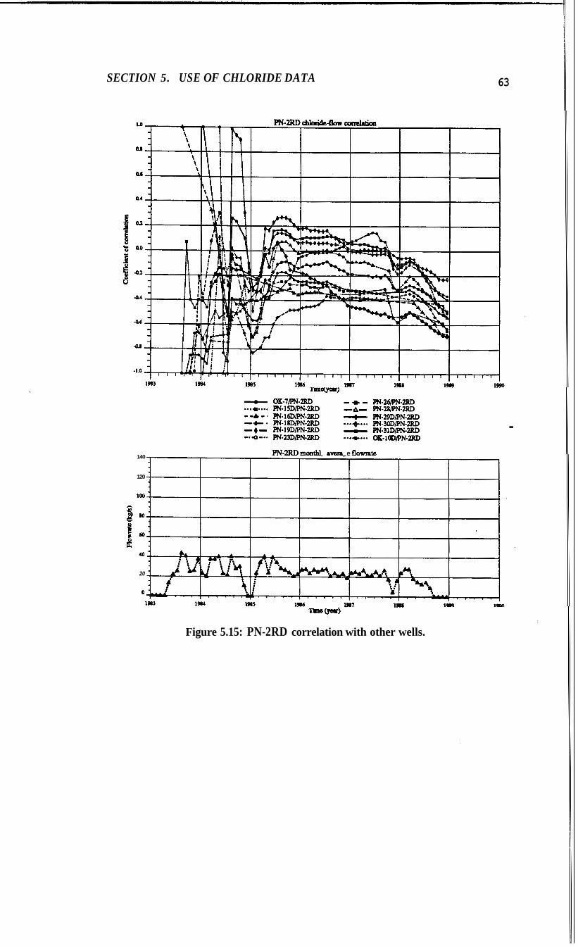
SECTION 5. USE OF CHLORIDE DATA 63
.
140 PN-2RD moathl a m e flowrate
120
100
b o
L f3
20
0
Figure 5.15: PN-2RD correlation with other wells.
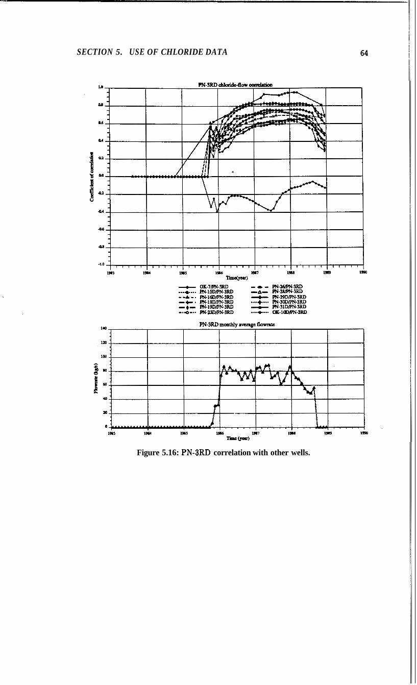
SECTION 5. USE OF CHLORIDE DATA 64
Figure 5.16: PN-3RD correlation with other wells.
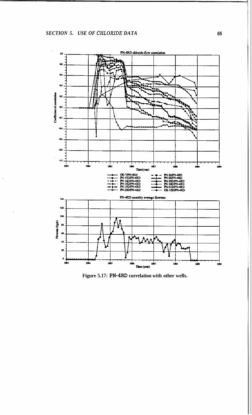
SECTION 5. USE OF CHLOMDE DATA 65
Figure 5.17: PN-4RD correlation with other wells.
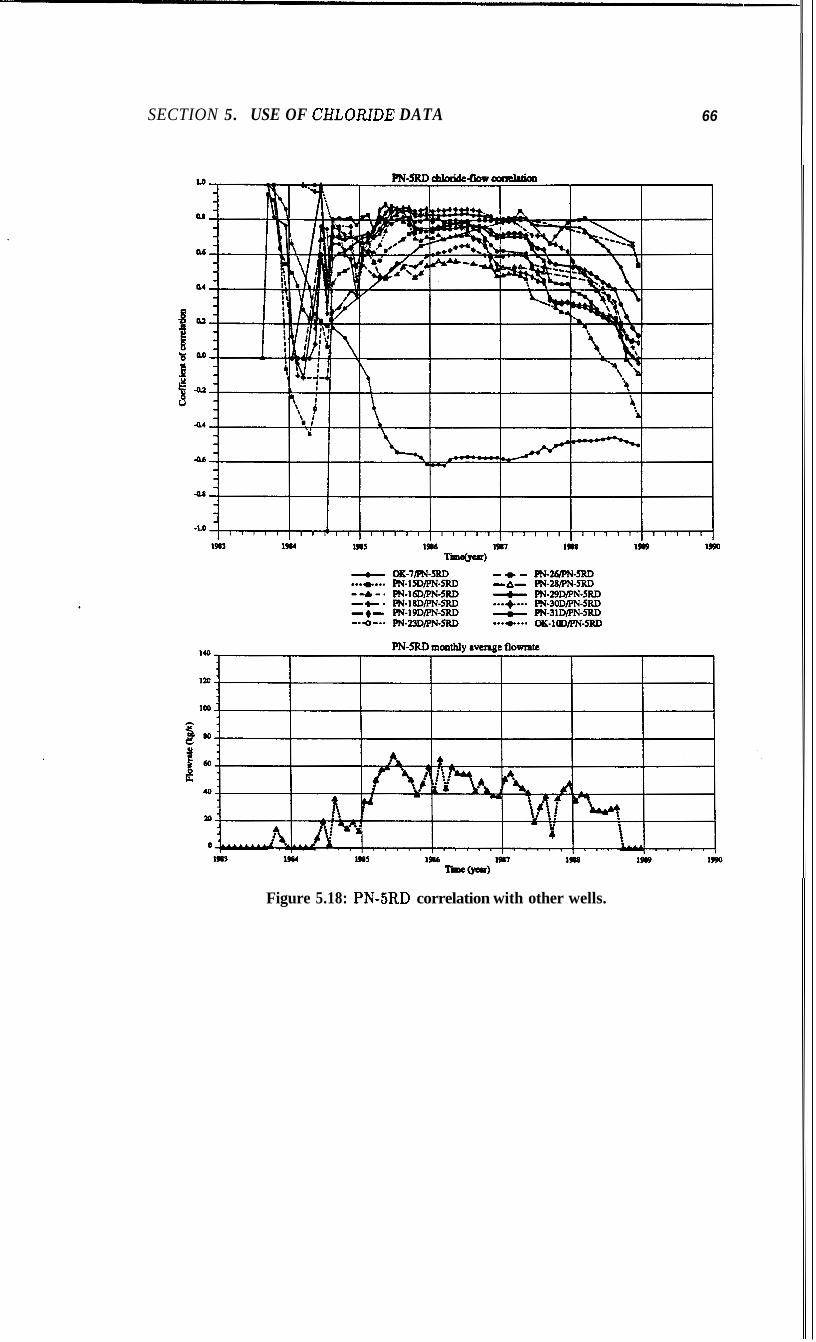
SECTION 5. USE OF CI-ILORlDE DATA 66
Figure 5.18: PN-5RD correlation with other wells.
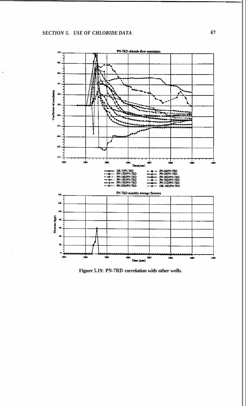
SECTION 5. USE OF CHLORIDE DATA 67
Figure 5.19: PN-7RD correlation with other wells.
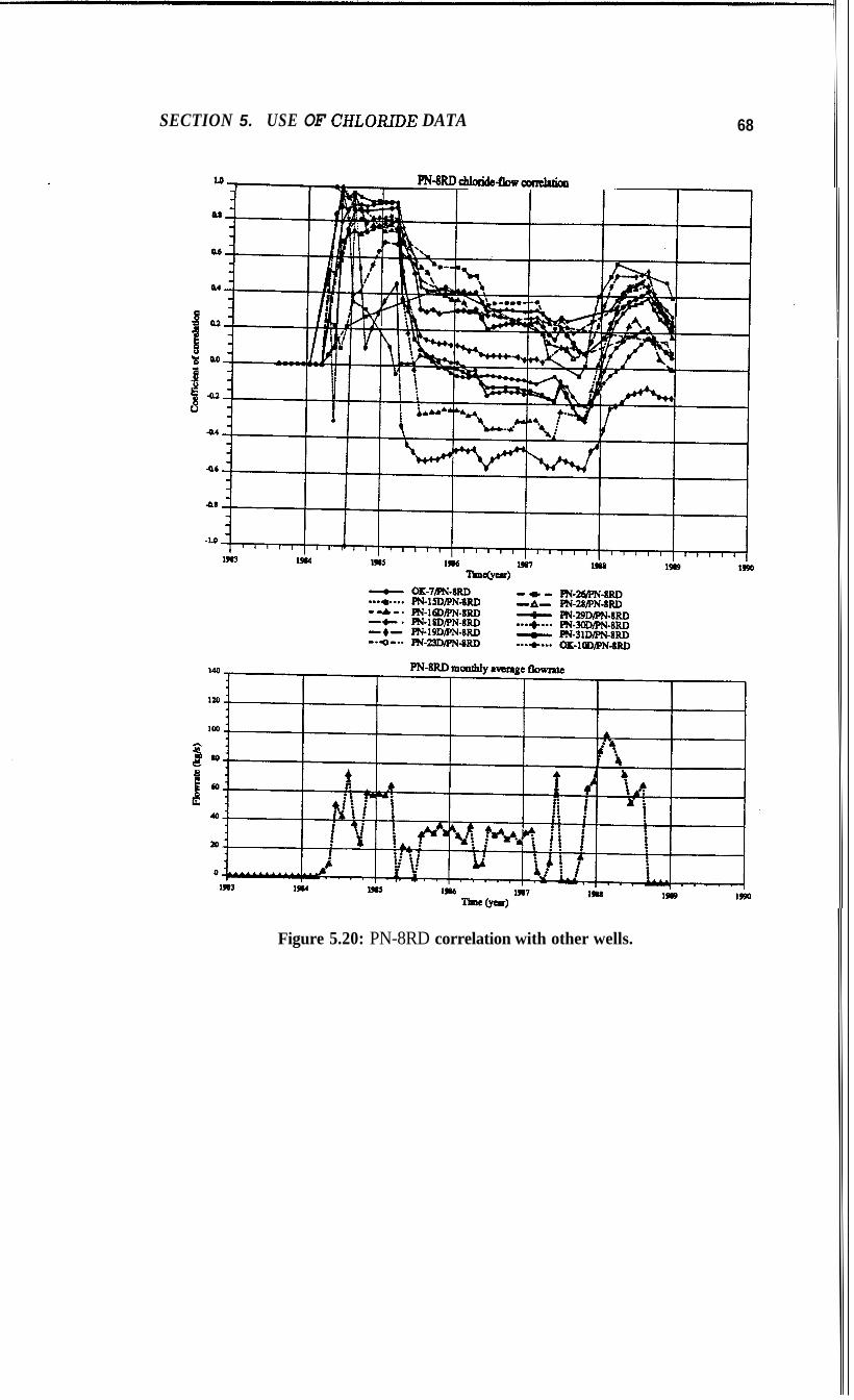
SECTION 5. USE OF CRLOR.DE DATA 68
Figure 5.20: PN-8RD correlation with other wells.
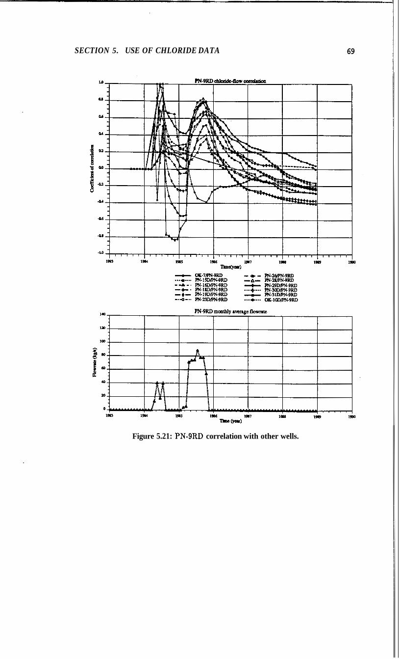
SECTION 5. USE OF CHLORIDE DATA 69
Figure 5.21: PN-9RD correlation with other wells.
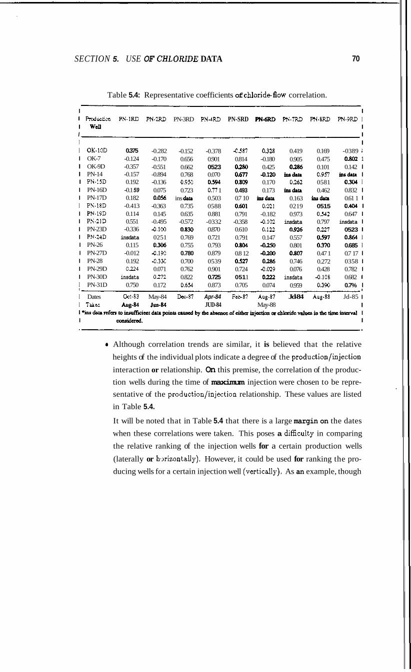
SECTION 5. USE OF CHLOR.DE DATA
Table 5.4: Representative coefficients of chlorideflow correlation.
70
I I I Reduction PN-1RD PN-2RD PN-3RD P N 4 D PN-SRD PN-6RD PN-7RD PN-8RD PN-9RD I I Wd I I I I I OK-10D I OK-7 I OK-9D I PN-14 I PN-15D I PN-16D I PN-17D I PN-18D I PN-19D I PN-2lD I PN-23D I PN-24D I PN-26 I PN-27D I PN-28 I PN-29D I PN-30D I PN-31D
0.375 -0.124 -0.357 -0.157 0.192 -0.1 59 0.182
-0.413 0.114 0.551
-0.336 insdata
0.115 -0.012 0.192 0.224
insdata 0.750
-0.282 -0.152 -0.170 0.656 -0.551 0.662 -0.894 0.768 -0.136 0950 0.075 0.723 0.056 ins data
-0.363 0.735 0.145 0.635
-0.495 -0.572 -0.100 0.830 0251 0.769 0.306 0.755
-0.190 0.780 -0330 0.700 0.071 0.762 0.272 0.822 0.172 0.654
-0.378 0.901 0523 0.070 0.594 0.77 1 0.503 0588 0.881
-0332 0.870 0.721 0.793 0.879 0539 0.901 0.725 0.873
I -0587 0328 0.419 0.169 -0389 1 0.814 0280
0.809 0.493 0.7 10 0.601 0.791
-0.358 0.610 0.791 0.804 0.8 12 0527 0.724 051 1 0.705
0.677
-0.180 0.425
0.170 0.173 ins&
0.021 -0.182 -0.102 0.122 0.147 -0.250 -0.200 0286
-0.029 0222 0.074
-0.m 0.905 0% inr&
0.262 ins&
0.163 0219 0.973
insdata 0.926 0.557 0.801 0.807 0.746 0.076
insdata 0.959
0.475 0.101 0.957 0581 0.462
insdate 0515 0542 0.797 0227 0597 0.370 0.47 1 0.272 0.428
-0.108 0390
0.802 0.142 ins&
0.304 0.832 0.61 1 0.404 0.647
insdata 0523 0.864 0.685 0.7 17 0358 0.782 0.682 0.7%
I
I Dates Oct-83 May-84 b87 Apr-84 F&87 Aug-87 Jd-84 Aug-88 Jd-85 I Taka JUD-84 May-88
I I
1 I I I I I I I I I I I I I I 1 I
I I I
I
0 Although correlation trends are similar, it is believed that the relative
heights of the individual plots indicate a degree of the production/injection
interaction or relationship. On this premise, the correlation of the produc- tion wells during the time of maximum injection were chosen to be repre- sentative of the production/injection relationship. These values are listed in Table 5.4.
It will be noted that in Table 5.4 that there is a large margin on the dates
when these correlations were taken. This poses a difEiculty in comparing
the relative ranking of the injection wells for a certain production wells
(laterally or hTnizontally). However, it could be used for ranking the pro- ducing wells for a certain injection well (vertically). As an example, though
SECTION 5. USE OF CHLORIDE DATA 71
the correlations for PN-lRD, PN-2RD, PN-4RD, PN-7RD, and PN-SRD, were taken in the years 1983-85, the correlations for PN-3RD, PN-GRD, and PN-8RD were taken in the latter years of 1987-88. This is due to the different periods of utilizing the reinjection wells. As a result, in the OK-7 row, it would not be possible to say that for OK-7, PN-4RD communicates stronger than PN-8RD since the coefficients were taken at disparate differ- ent times. But a look at the PN-9RD column would show the ranking to
be PN-24D, PN-16D, OK-7, PN-31D, PN-29D, PN-27D, PN-26, PN-SOD, PN-19D, PN-l7D, PN-18D, PN-28, PN-16D, OK-9D and finally, OK-1OD in order of decreasing correlation. These results would indicate that PN- 24D, PN-16D, and PN-27D are three. other wells which correlate highly
with PN-9RD aside from the wells monitored to do so during the PN-9RD tracer test. In the same fashion, the PN-1RD column would indicate that
the wells which correlate positively with it are PN-31D, PN-29D, PN-28, PN-l5D, PN-l7D, PN-26, and PN-19D. However, though these wells were
monitored in the sodium fluorescein test (see Table 3.1)) the dye was de- tected only in production wells PN-26, PN-28, and OK-7. The results,
therefore, of the chloride-flow correlation are not in substantial agreement
with the chemical tracer test. It will be noted that for the PN-6RD column,
the ranking of wells of OK-gD, OK-lOD, PN-28, PN-SOD, PN-16D, PN- 15D, PN-23D, and PN-31D are slightly different from the previous ranking provided by Table 5.3. The reason is that different times were considered
for the two tables and of the two, Table 5.4 covers a longer span of time.
0 It is evident, then, that the chloride-flow correlation method can rank pro- duction wells for each injection well but fails to rank the injection wells for each production well. In other words, the method fails to distinguish or separate the individual contributions of the injection wells for a par-
ticular production well especially when the the injection wells are used simultaneously in the same time.
SECTION 5. USE OF CHLORIDE DATA 72
5.2 Chloride = Cumulative Flowrate Correla-
t ion
Another method used was to investigate the correlation between the production
chloride value and the cumulative injection flowrate. Since the chloride value of a production well at a particular time is an accumulated effect, it would seem reasonable to see the relationship between this chloride value and the cumulative
flowrate of the injection well. This means that the injection flowrate is summed
with time and the cumulative flowrate at any given time is correlated with the production chloride value.
Figures 5.22 and 5.23 illustrate the methods on OK-7IPN-SRD and PN-l7D/PN- 6RD pair of wells, while Figure 5.24 shows the results on wells PN-26, PN- 28, and PN-29D. Other plots are given in Appendix H. It can be seen from
Figures 5.22 and 5.23 that the correlation values of OK-7/PN-9RD and PN- 17D/PN-6RD are always positive and generally high. This is a r m e d by Fig- ure 5.24 which shows consistently high positive values for the production wells regardless of the injection well correlated with. Upon examination, this can be
explained by the fact that when the injection flowrates are summed, the result- ing increasing flowrates are correlated with increasing chloride values, too. The
outcomes, therefore, are high positive values of correlation. For this reason,
this method has been disregarded as an effective tool of determining produc- tion/injection relationship.
5.3 Chloride Deviation = Flowrate Correlation
The purpose of the third method was to examine the relationship between the magnitude of the increases in the chloride value of a producing well with
the injection flowrates. If there is a strong communication between a pair
of producer and injector, it would be logical to expect that the effect of a high injection rate would be a greater step change in the chloride value of the
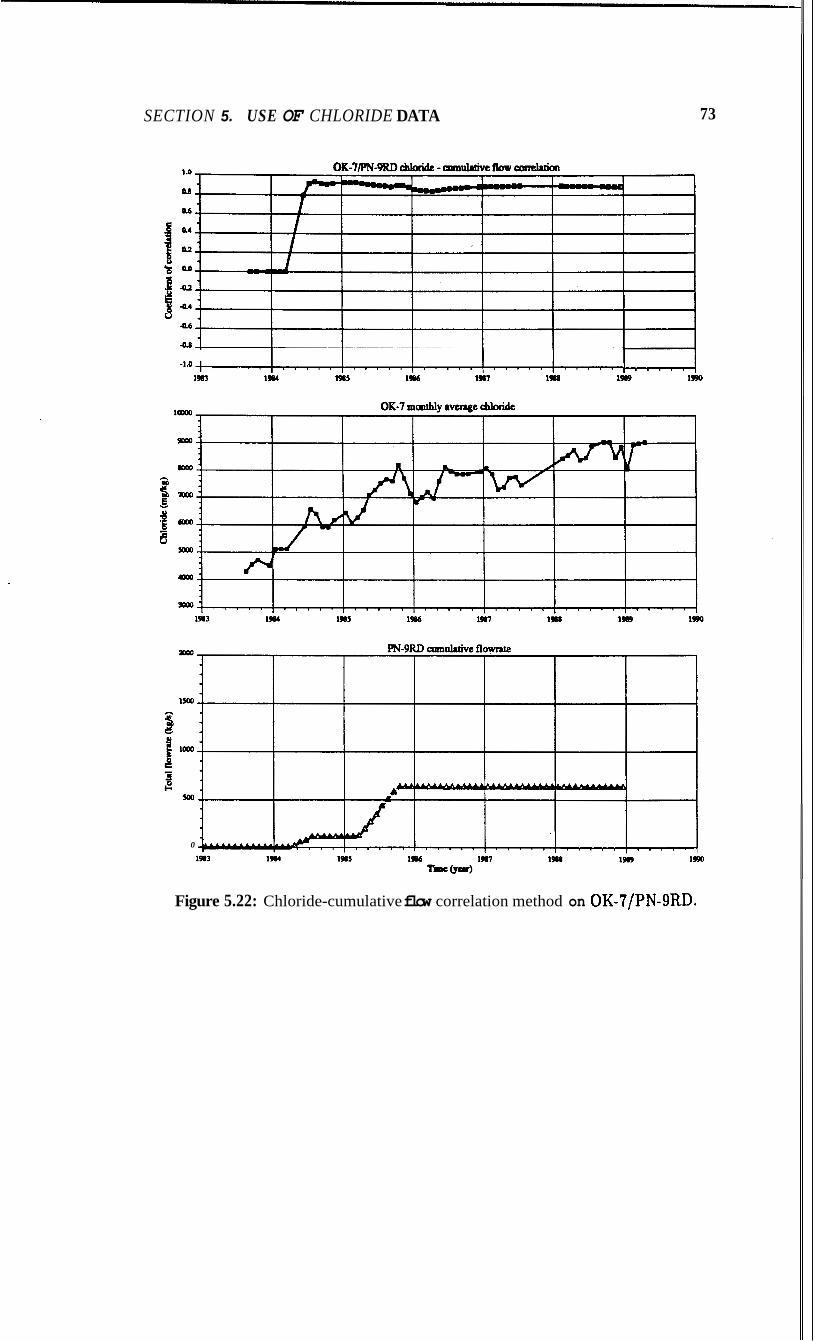
SECTION 5. USE OF CHLORIDE DATA 73
-1.0 , , I . . , * , / 1 ~ " " I " " ' I ' " ' ' I ' " ' ' I ' " " I
1963 19U 1985 19M 1y07 1- 19(9 1990
0
Figure 5.22: Chloride-cumulative flow correlation method on OK-7/PN-SRD.
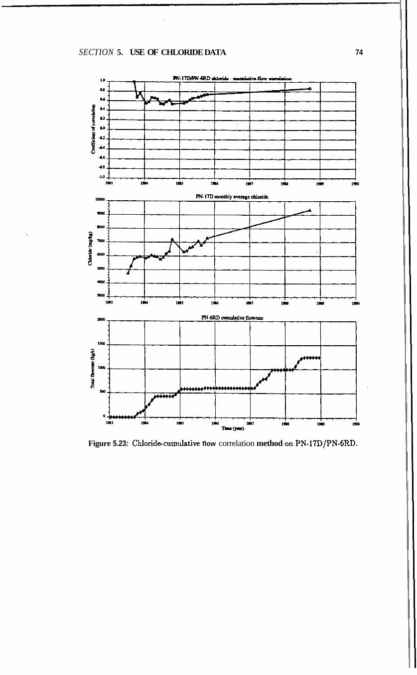
SECTION 5. USE OF CHLORIDE DATA 74
1983
Figure 5.23: Chloridwxmulative flow correlation method on PN-1'7DIPN-GRD.
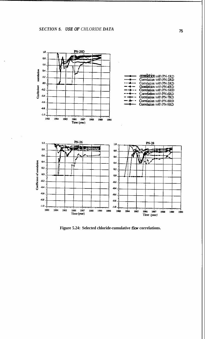
SECTION 5. USE OF CHLORIDE DATA 75
1 .o PN-29D
0.6
.g a4 1 02
ao
‘G Qz 8 8 a 4
1
u -0.6
-0.8
-1.0
correlation with PN-1RD Carrelation with PN-2RD Carrelatian with PN-3RD
Correlatio~l with PN-SRD
Correlati~n with PN-7RD COrrelati~n with PN-8RD hhti~n with PN-9RD
Correlation with PN4RD
Correlation with P N W
1983 1984 1985 1986 1987 Time (ycar)
1988 1989 1990
Time (year)
Figure 5.24: Selected chloride-cumulative flow correlations.
SECTION 5. USE OF CHLORIDE DATA 76
producing well. To measure this change, it was assumed that the trend of increasing chloride values can be represented by a linearly regressed line. The magnitude of the change is measured by the deviation of the chloride value
from this best fit line and this chloride deviation was, then, correlated with the injection flowrate. Appendix J lists the program for calculating the coefficient
of correlation after finding the chloride deviation from the best fit line using linear regression.
Figure 5.25 shows an example of the measured chloride values and the computed
best fit line. Figure 5.25 shows successively, the injection flowrates of PN- 9RD, the calculated chloride deviation from the linearly regressed line, and the
resulting correlation values. It is interesting to note that the chloride deviation values from the best fit, line are greatest and coincident with the injection of PN-9RD. Because of this, the correlation values are high and increasing during these periods of excellent accord between the injection flowrates and the chloride changes.
The correlations for the rest of the PN-9RD production wells were calculated
using this method and the results are plotted in Figure 5.27. It can be seen that the general shapes of the correlation plots using the two methods are generally similar. However, upon closer examination it appears that the chloride-flow
correlation values simulate better the results of the tracer test. As an example, the chloride-flow correlation method shows only OK-1OD to be negatively cor- related for the second wave of PN-9RD injection. This is consistent with the results of the PN-9RDtracer test. On the other hand, the chloride deviation-
flowrate method registers OK-lOD, PN-17D, PN-28, and PN-18D to be nega-
tively correlated with PN-9RD in contrast to the tracer results.
Figure 5.28 shows the result of the chloride deviation- flowrate method on PN-
17D and PN-6RD and Figure 5.29 shows the correlation plots of the two meth- ods. As in the PN-SRD, the results indicate the chloride-flow correlation to be more reflective of the PN-6RD relationship with these producing wells. To illus-
trate, the plots of OK-7 and PN-28 are sensitive to the use of PN-6RD for the
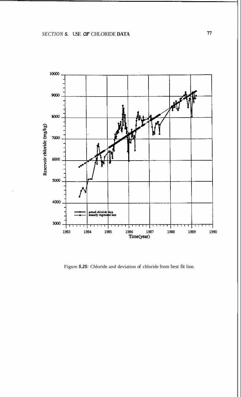
SECTION 5. USE OF CHLORIDE DATA 77
loo00
8000
7000
5000
4000
1983 1984 1985 1986 1987 1988 1989 1990 Timebear)
Figure 5.25: Chloride and deviation of chloride from best fit line.
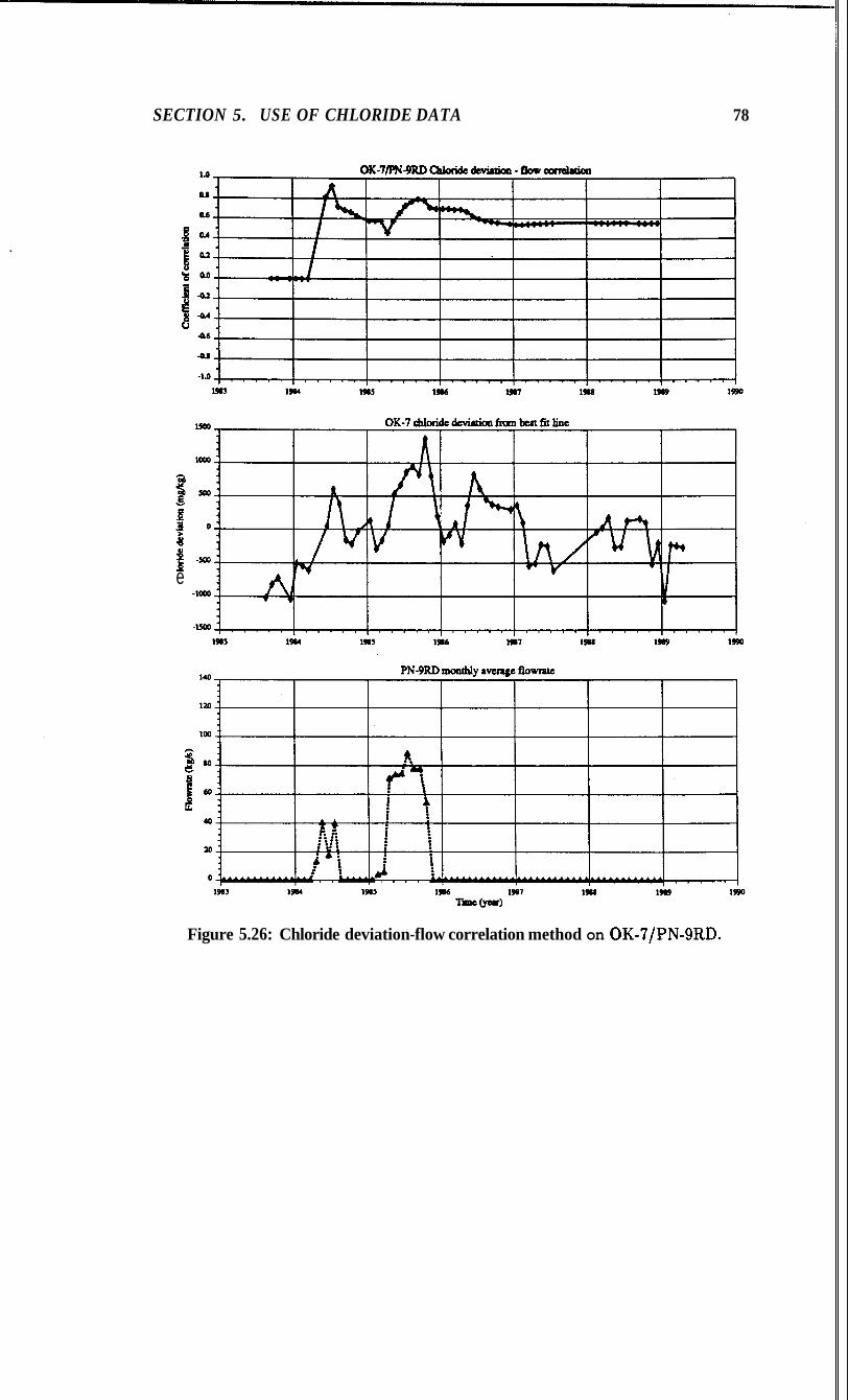
SECTION 5. USE OF CHLORIDE DATA 78
wo
.$
b 3 0
f -m e
-1000
-wo 1983
Figure 5.26: Chloride deviation-flow correlation method on OK-7/PN-SRD.
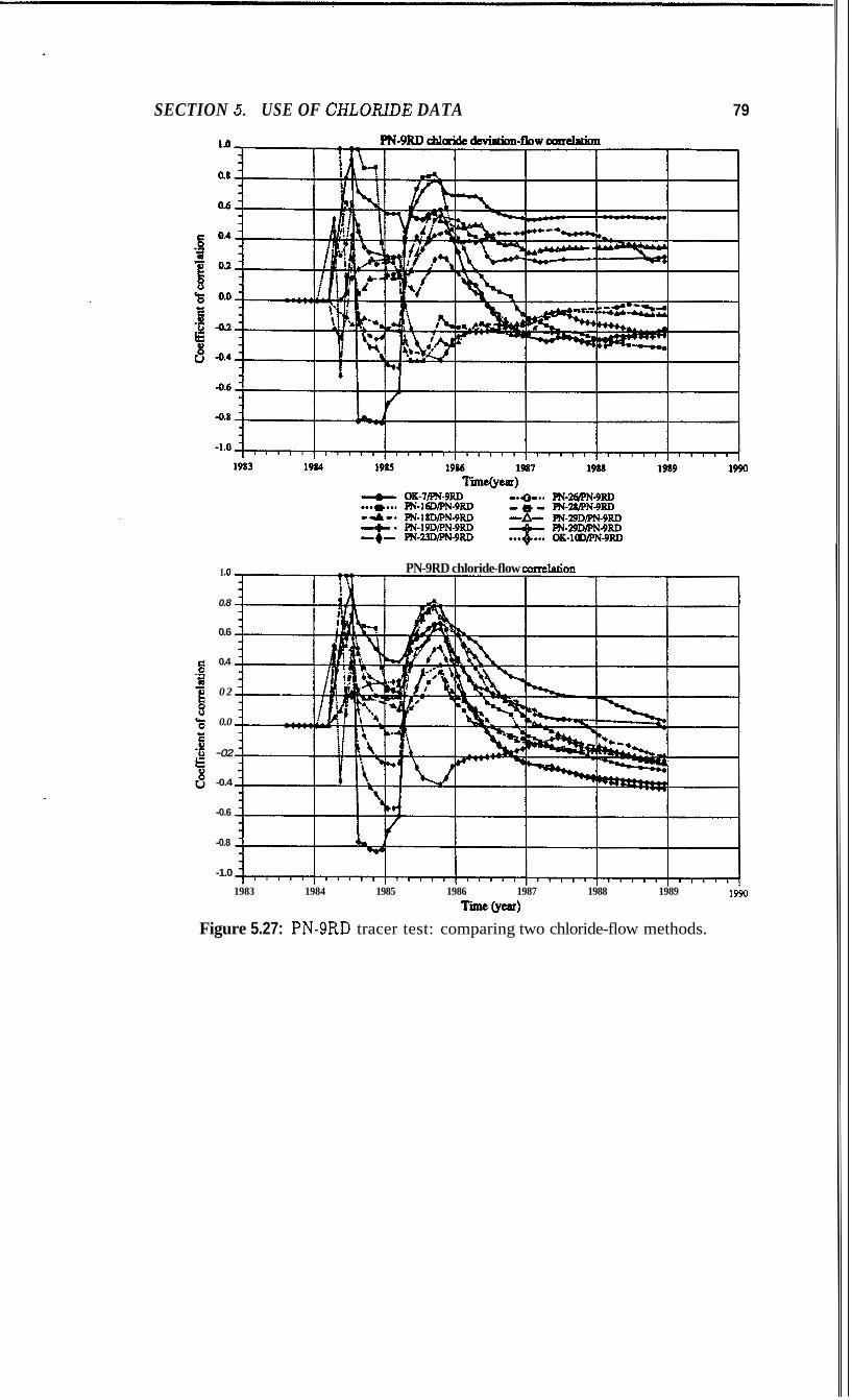
SECTION 5. USE OF CHLORJDE DATA 79
1 .o
0.8
0.6
0.4
0 2
0.0
-02
-0.4
-0.6
-0.8
-1.0
PN-9RD chloride-flow amelation
1983 1984 1985 1986 1987 1988 1989 1990 Ti= 6-d
Figure 5.27: PN-9RD tracer test: comparing two chloride-flow methods.
SECTION 5. USE OF CHLORIDE DATA 80
chloride-flow correlation but behave otherwise in the chloride deviation-flowrate
correlation. Appendix I shows the plots for the rest of the injection wells using
the two correlation methods. The same features are exhibited by these plots as has been discussed for the PN-9RD and the PN-6RD cases.
Therefore, it can be concluded that the chloride-flow correlation method is a
better indicator of the strength of the producer/injector relationship.
5.4 Linear Combination Met hod
The preceding sections have discussed the results of getting the correlation by using the chloride values of a production well and the flowrates of a particular
injection well. Of the three methods, the chloride-flow correlation method shows
merit in ranking the production wells for a certain injection well. It is, however,
limited in its capability to rank the injection wells for a production well since it fails to distinguish the individual contributions from the injection wells.
To take into account the reality that the net effect on a production well is due to the effects of the particular injection wells which were active during the time, the last method expresses the chloride value of the producing well as a linear combination of the injection flowrates of the all the active reinjection wells at
the particular time considered. In mathematical symbols, this can be written:
where n = number of reinjection wells chosen
i = number of particular time set considered
Cl i = chloride value of well at time i
qni = injection flowrate of well n at time i
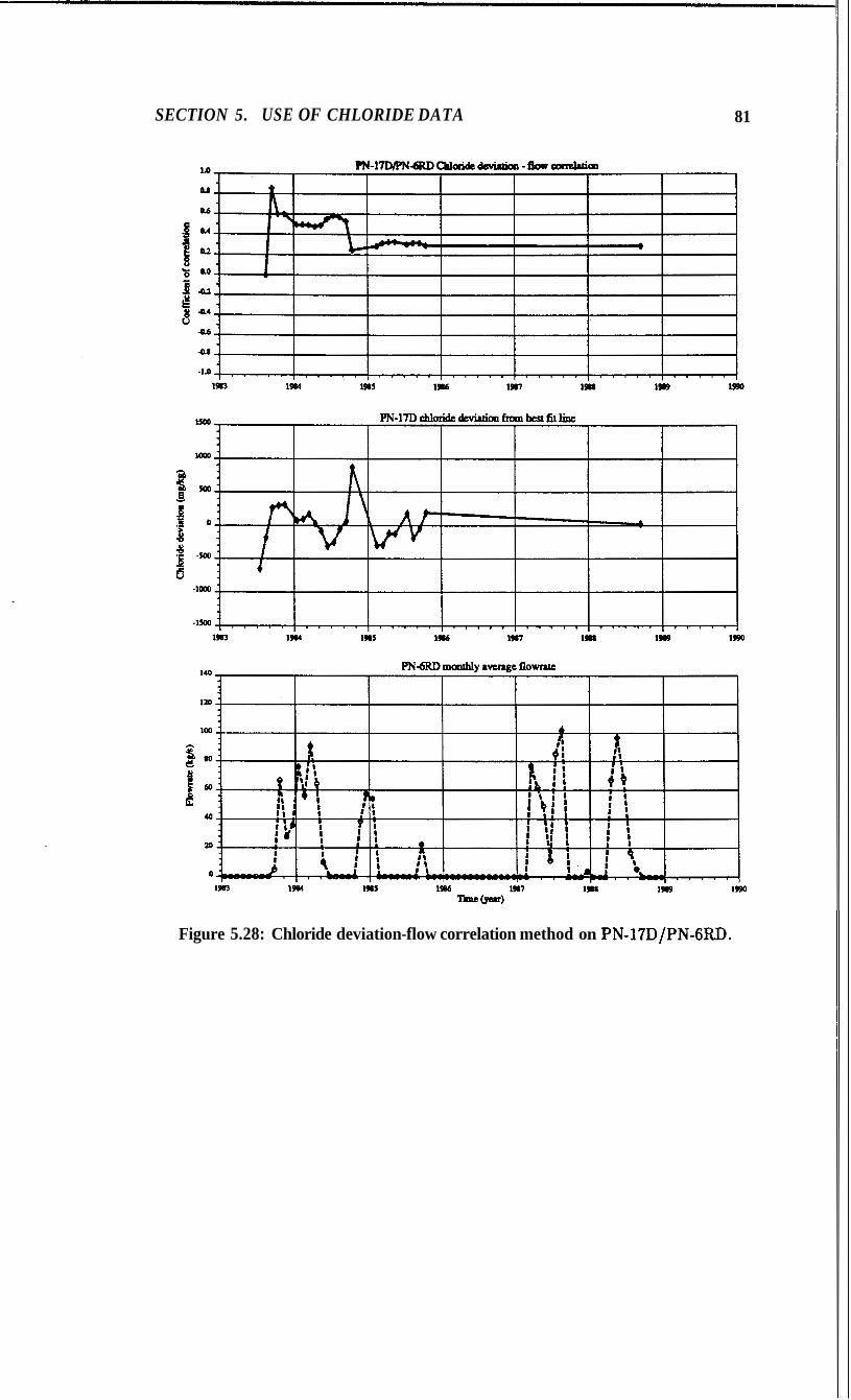
SECTION 5. USE OF CHLORIDE DATA 81
Figure 5.28: Chloride deviation-flow correlation method on PN-17D/PN-GRD.

SECTION 5. USE OF CHLORIDE DATA 82
1.0
0.8
0.6
0.4
0.2
0.0
-0.2
0.4
-0.6
-0.8
-1.0
Figure
1 .o PN-6RD chloride-flow corre 0
0.8
0.6
0.4
0.2
0.0
-02
-0.4
-0.6
-0.8
-1.0
1983 1984 1985 1986 1997 1988 1989 1990 Time (year)
5.29: OK-12RD/PN-GRD tracer test: comparing two chloride-flow methods.
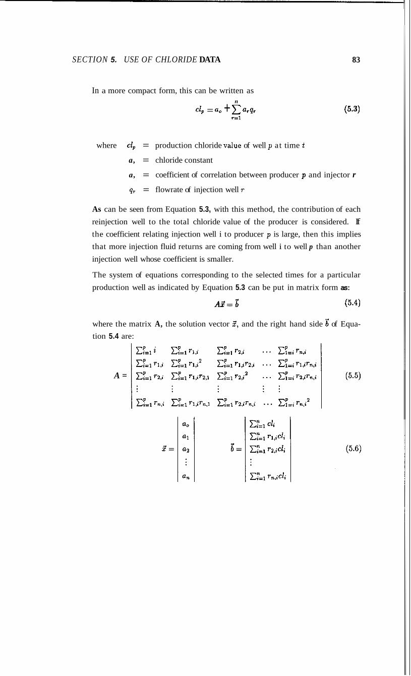
SECTION 5. USE OF CHLORIDE DATA 83
In a more compact form, this can be written as n
C I p = a0 + arqr ,=l
(5.3)
where cZp = production chloride value of well p at time t
a, = chloride constant
a, = coefficient of correlation between producer p and injector r
q, = flowrate of injection well r
As can be seen from Equation 5.3, with this method, the contribution of each reinjection well to the total chloride value of the producer is considered. If the coefficient relating injection well i to producer p is large, then this implies that more injection fluid returns are coming from well i to well p than another injection well whose coefficient is smaller.
The system of equations corresponding to the selected times for a particular production well as indicated by Equation 5.3 can be put in matrix form as:
AZ= (5.4)
where the matrix A, the solution vector 5, and the right hand side of Equa- tion 5.4 are:
A =
...
X = -#

SECTION 5. USE OF CHLOMDE DATA 84
The solution to these simultaneous linear equations is solved by a matrix solver which used the Gauss-Jordan method. It has been modified so that the con- stant a, takes on the chloride value at the initial time defined. Sometimes, it
may happen that the matrix A is singular which means no solution exists to the
system of equations. In this instance, the program prints a “no solution” mes-
sage. Appendix K gives the source program listing and an example of aa output which gives the coefficients for the time interval and injection wells specified by the user.
5.4.1 Results Using Whole Data Set
As the title suggests, the coefficients of correlation were calculated for the Pal- inpinon production wells using all the injection wells from August 1983 to De- cember 1988. The results are given by Table 5.5.
Table 5.5 has been put in horizontal stacked bar forms (Figures 5.30 and 5.31) in order to see more clearly the contributions of each reinjection well to a pro-
duction well (row analysis) and the production wells affected in varying degrees
by each injection well (columnar analysis). Each bar corresponds to a row of coefficient values which are horizontally stacked to make up the total bar. These
bars represent only wells with positive correlations, and therefore, the absentee
wells are those of negative correlation with either the production or reinjection well, as the case may be.
From Figures 5.30 and 5.31, the following aspects have been observed and de- termined:
0 The different contributions of the reinjection wells to a particular produc- tion wells are now separated and made distinguished. As an example. it
can been from the stacked bar of PN-29D that this well is strongly influ- enced by PN-SRD, followed by PN-SRD, PN-SRD, PN-lRD, PN-4RD, and
PN-6RD. The rest of the injection wells do not correlate positively with PN-29D.
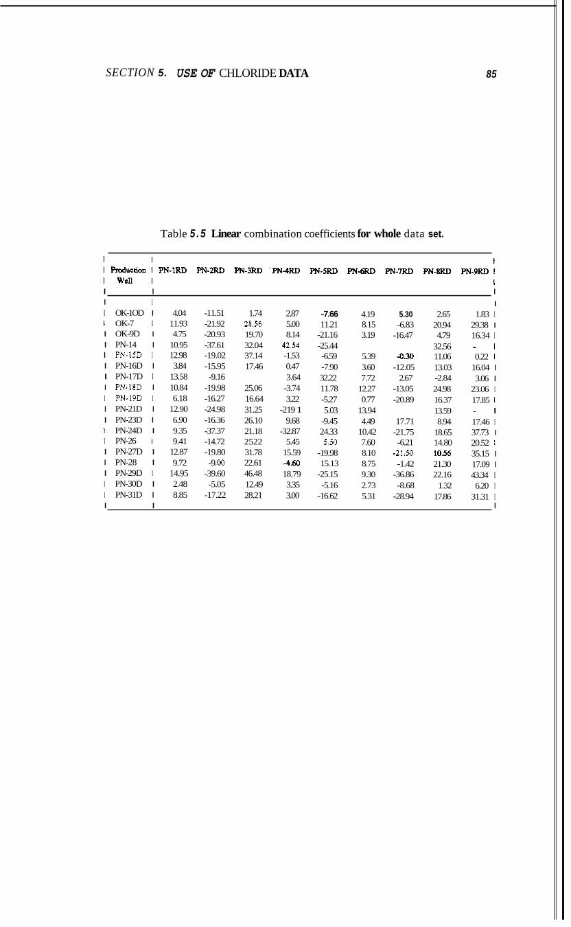
SECTION 5. USE OF CHLORIDE DATA
Table 5 . 5 Linear combination coefficients for whole data set.
85
I I I I I I OK-1OD I I OK-7 I I OK-9D I I PN-14 I I PN-15D I I PN-16D I I PN-17D I I PN-18D I I PN-19D I I PN-21D I I PN-23D I 1 PN-24D I I PN-26 I I PN-27D I I PN-28 I I PN-29D I I PN-30D I I PN-31D I
4.04 11.93 4.75
10.95 12.98 3.84
13.58 10.84 6.18
12.90 6.90 9.35 9.41
12.87 9.72
14.95 2.48 8.85
-11.51 -21.92 -20.93 -37.61 -19.02 -15.95 -9.16
-19.98 -16.27 -24.98 -16.36 -37.37 -14.72 -19.80 -9 .oo
-39.60 -5.05
-17.22
1.74 28.56 19.70 32.04 37.14 17.46
25.06 16.64 31.25 26.10 21.18 2522 31.78 22.61 46.48 12.49 28.21
2.87 5.00 8.14
42.54 -1.53 0.47 3.64
-3.74 3.22
-21 9 1 9.68
-32.87 5.45
15.59 4.60 18.79 3.35 3.00
-7.66 11.21
-21.16 -25.44 -6.59 -7.90 32.22 11.78 -5.27 5.03
-9.45 24.33 5.50
-19.98 15.13
-25.15 -5.16
-16.62
4.19 8.15 3.19
5.39 3.60 7.72
12.27 0.77
13.94 4.49
10.42 7.60 8.10 8.75 9.30 2.73 5.31
5.30 -6.83
-16.47
-0.30 -12.05
2.67 -13.05 -20.89
17.71 -21.75 -6.21
-21.50 -1.42
-36.86 -8.68
-28.94
2.65 20.94 4.79
32.56 11.06 13.03 -2.84 24.98 16.37 13.59 8.94
18.65 14.80 10.56 21.30 22.16
1.32 17.86
I 1.83 I
29.38 I 16.34 I - I 0.22 I
16.04 I 3.06 I
23.06 I 17.85 I - I 17.46 I 37.73 I 20.52 I 35.15 I 17.09 I 43.34 I 6.20 I
31.31 I I I I
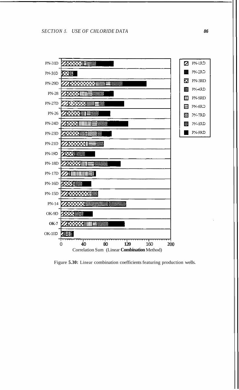
SECTION 5. USE OF CHLORIDE DATA 86
PN-3 1 D
PN30D
PN-29D
PN-28
PN-27D
PN-26
PN-24D
PN-23D
PN-21D
PN- 19D
PN- 18D
PN- 17D
PN- 16D
PN- 15D
PN- 14
OK-9D
OK-7
OK- 10D
0 40 80 120 160 2 Correlation Sum (Linear Combination Method)
PN- 1RD
PN-2RD
PN-3RD
PN4RD
PN-SRD
PN-6RD
PN-7RD
PN-8RD
PN-9RD
Figure 5.30: Linear combination coefficients featuring production wells.
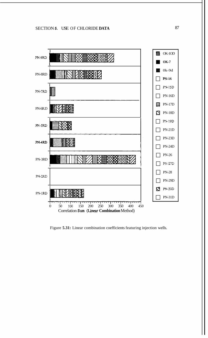
SECTION 5. USE OF CHLORIDE DATA 87
I PN-9RD
I
I PN-8RD
PN-7RD
PN-6R.D
PN-SRD
PN-3RD
PN-2RD
PN- 1 R D
I 1 " " 1 ' " ' 1 " " 1 " " I " " I ' " ' I " ' ' l " ' ' l ' " ' l
Correlation Sum (Lmear Combination Method) 0 50 100 150 200 250 300 350 400 450
OK-1OD
OK-7
0k-9d
~ ~ - 1 4
PN-15D
PN-16D
PN-17D
63 PN-18D
PN-19D
PN-21D
PN-23D
PN-24D
PN-26
PN-27D
PN-28
PN-29D
PN-30D
PN-31D
Figure 5.31: Linear combination coefficients featuring injection wells.
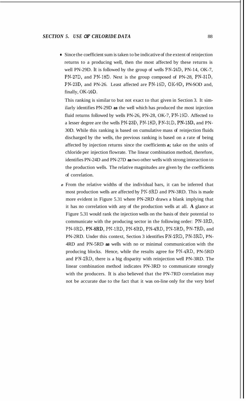
SECTION 5. USE OF CHLORIDE DATA 88
0 Since the coefficient sum is taken to be indicative of the extent of reinjection
returns to a producing well, then the most affected by these returns is well PN-29D. It is followed by the group of wells PN-24D, PN-14, OK-7, PN-27D, and PN-18D. Next is the group composed of PN-28, PN-31D, PN-23D, and PN-26. Least affected are PN-16D, OK-gD, PN-SOD and, finally, OK- 10D.
This ranking is similar to but not exact to that given in Section 3. It sim-
ilarly identifies PN-29D as the well which has produced the most injection
fluid returns followed by wells PN-26, PN-28, OK-7, PN-19D. Affected to a lesser degree are the wells PN-23D, PN-l$D, PN-31D, PN-l5D, and PN-
30D. While this ranking is based on cumulative mass of reinjection fluids discharged by the wells, the previous ranking is based on a rate of being affected by injection returns since the coefficients a; take on the units of chloride per injection flowrate. The linear combination method, therefore,
identifies PN-24D and PN-27D as two other wells with strong interaction to
the production wells. The relative magnitudes are given by the coefficients
of correlation.
0 From the relative widths of the individual bars, it can be inferred that most production wells are affected by PN-9RD and PN-3RD. This is made more evident in Figure 5.31 where PN-2RD draws a blank implying that it has no correlation with any of the production wells at all. A glance at
Figure 5.31 would rank the injection wells on the basis of their potential to
communicate with the producing sector in the following order: PN-3RD,
PN-SRD, PN-8RD, PN-lRD, PN-GRD, PN4RD, PN-5RD, PN-7RD, and
PN-2RD. Under this context, Section 3 identifies PN-2RD, PN-SRD, PN-
4RD and PN-5RD as wells with no or minimal communication with the
producing blocks. Hence, while the results agree for PN-4RD, PN-5RD and PN-2RD, there is a big disparity with reinjection well PN-3RD. The linear combination method indicates PN-3RD to communicate strongly
with the producers. It is also believed that the PN-7RD correlation may not be accurate due to the fact that it was on-line only for the very brief
SECTION 5. USE OF CHLORIDE DATA 89
period of May-July 1984 and consequently, contributed only three data
points for the whole time considered.
At this junction, it would be interesting to compare the results of the linear
combination method with the chloride-flow method for the tracer tests, in par-
ticular, and as a whole in general.
Table 5.6 shows how the monitored production wells were ranked according to the tracer tests, the chloride-flow correlation method and the linear combination method. There are differences in the three columns on the ranking of the
wells. While the chloride-flow method ranks OK-7 first in agreement with the tracer result, the linear combination method ranks PN-29D first. In terms of relative ranking of the production wells, the chloride-flow method is closer to
the tracer data. For the OK-12RD/PN-GRD, the production wells affected are
in agreement but the relative ranking is not.
Since it has been stated that one deficiency of the chloride-flow method is the inability to distinguish the different contributions of the reinjection wells to a particular production well, comparison will be made between the reinjection wells and the production wells communicated with. Table 5.7 is a coalescence
of Table 5.4 of the chloride-flow correlation method and Table 5.5 of linear com-
bination method. Figure 5.32 shows the results of the chloride-flow correlation
method drawn from Table 5.7.
When Figure 5.32 is compared to Figure 5.31, the following similarities and differences are noted:
0 Both figures have injection well PN-2RD as communicating least with the
producers. But while the linear combination method has negative corre-
lations for PN-2RD, the chloride-flow method has positive, although low correlations, of PN-2RD with PN-26, PN-24D, PN-SOD, PN-31D, and PN- 19D.
0 The linear combination has ranked PN-3RD, PN-SRD, PN-8RD, and PN-
1RD as the first four most “harmful” wells. The chloride-flow method has
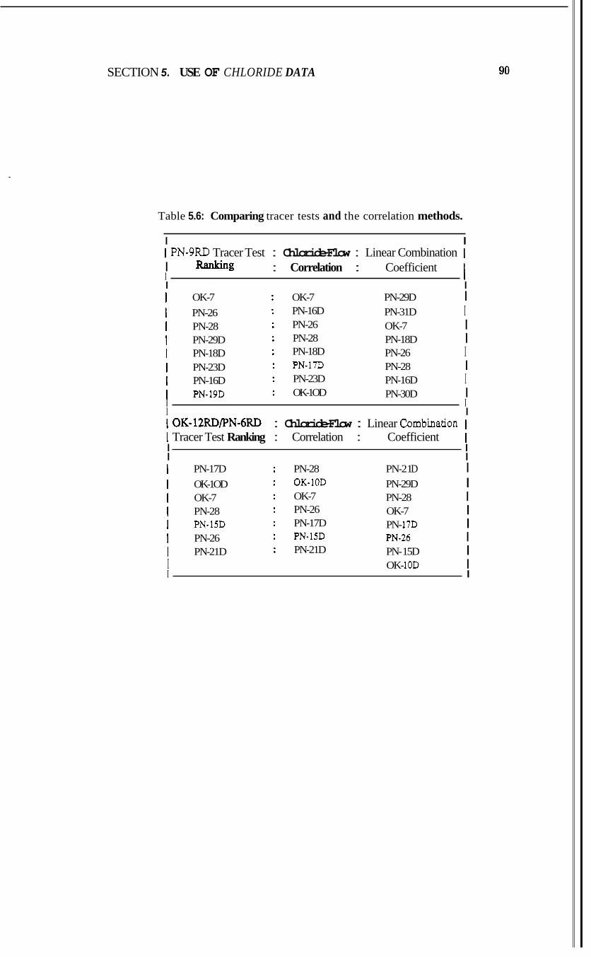
SECTION 5. USE OF CHLORIDE DATA
Table 5.6: Comparing tracer tests and the correlation methods.
I I I PN-9RD Tracer Test : Chloride-Flow : Linear Combination I
I 1 I I I OK-7 : OK-7 PN-29D I I PN-26 : PN-16D PN-31D I I PN-28 : PN-26 OK-7 I I PN-29D : PN-28 PN-18D I I PN-18D : PN-18D PN-26 I I PN-23D : PN-17D PN-28 I I PN-16D PN-23D PN-16D I I PN-19D : OK-1OD PN-30D I I I I I I OK-12RDPN-6RD : Chloride-Flow : Linear Combination I I Tracer Test Ranking : Correlation : Coefficient I I I I I I PN-17D : PN-28 PN-2 1 D I I OK-1OD : OK-10D PN-29D I I OK-7 : OK-7 PN-28 I I PN-28 : PN-26 OK-7 I I PN-15D : PN-17D PN- 17D I I PN-26 : PN-15D PN-26 I I PN-21D : PN-21D PN- 15D I
I I
I Ranking : Correlation : Coefficient I
I OK- 1OD I
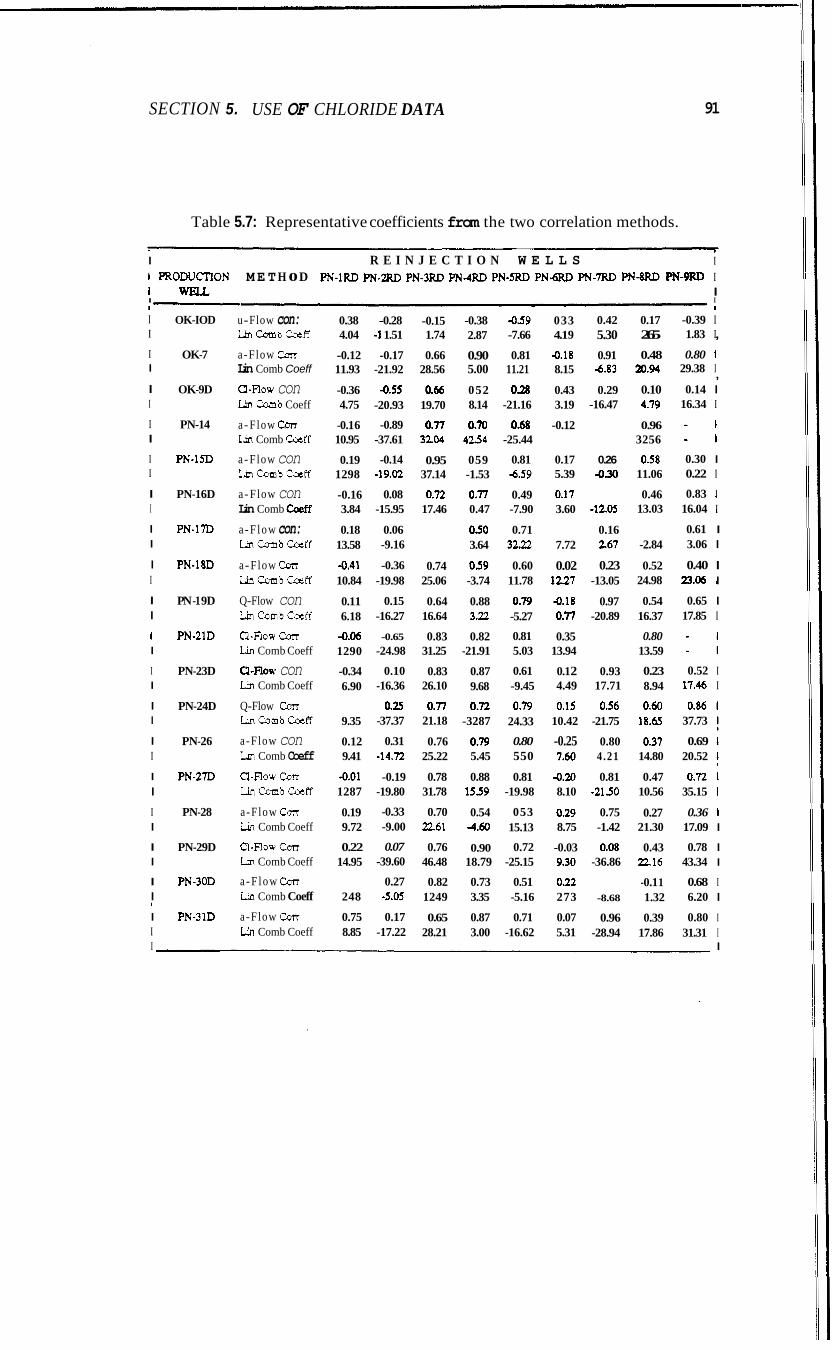
SECTION 5. USE OF CHLORIDE DATA 91
Table 5.7: Representative coefficients from the two correlation methods.
I
I R E I N J E C T I O N W E L L S I 1 PRODUCIlON M E T H 0 D PN-1RD PN-pu) PN-3RD PN-4RD PN-5RD F'N- PN-7RD PN4RD PN-9RD I I W E L L I
~ ~~~~~~ ~~ ~~
I I 1 1
I I
I I
I I
I I
I I
I I
I I
I I
I I
I I
I I
I I
I I
I I
I I
I I
I I
I I
0
OK-IOD
OK-7
OK-9D
PN-14
PN-15D
PN-16D
PN-17D
PN-18D
PN -1 9D
PN-2lD
PN-23D
PN-24D
PN-26
PN-27D
PN-28
PN-29D
PN3OD
PN91D
u-Flow con: Lin-bCoeff
a-Flow coa Lin Comb Coeff
a-Flow con Lin m b Coeff
a-Flow CmI Lin Comb Cocff
a-Flow con LinCombCotff
a-Flow con Lin Comb coeff a - F low con: LinCombCotff
a-Flow carr LinCombCoeff
Q-Flow con LinCombCoeff
Q-Flow con: Lin Comb Coeff
a-Flow con Lin Comb Coeff
Q-Flow CmI LinCombCotff
a-Flow con Lin Comb Coeff a m o w corr LinCombCoeff
a-Flow corr Lin Comb Coeff
a - R o w carr Lin Comb Coeff
a - F low con: Lin Comb Coeff
a-Flow con Lin Comb Coeff
0.38 4.04
-0.12 11.93
-0.36 4.75
-0.1 6 10.95
0.19 1298
-0.16 3.84
0.18 13.58
-0.41 10.84
0.11 6.18
-0.06 1290
-0.34 6.90
-0.28 -1 1.51
-0.17 -21.92
-0.55 -20.93
-0.89 -37.61
-0.14 -19.02
0.08 -15.95
0.06 -9.16
-0.36 -19.98
0.15 -16.27
-0.65 -24.98
0.10 -16.36
-0.15 -0.38 1.74 2.87
0.66 0.90 28.56 5.00
0.66 052 19.70 8.14
0.77 0.70 3204 42.54
0.95 059 37.14 -1.53
0.72 0.77 17.46 0.47
050 3.64
0.74 059 25.06 -3.74
0.64 0.88 16.64 3x2
0.83 0.82 31.25 -21.91
0.83 0.87 26.10 9.68
4.59 -7.66
0.81 11.21
0.28 -21.16
0.68 -25.44
0.81 4.59
0.49 -7.90
0.71 32.22
0.60 11.78
0.79 -5.27
0.81 5.03
0.61 -9.45
033 4.1 9
4.18 8.15
0.43 3.19
-0.12
0.17 5.39
0.17 3.60
7.72
0.02 12.27
-0.18 0.77
0.35 13.94
0.1 2 4.49
0.42 5.30 0.91
4.83
0.29 -16.47
0.26 -0.30
-1205
0.16 267
0.23 -13.05
0.97 -20.89
0.93 17.71
0.17 265
0.48 20.94
0.10 4.79
0.96 3256
A58 11.06
0.46 13.03
-2.84
0.52 24.98
0.54 16.37
0.80 13.59
0.23 8.94
-0.39 I 1.83 I , 0.80 1
29.38 I
0.14 I 16.34 I
* I - I
0.30 I 0.22 I
0.83 1 16.04 I I
0.61 I 3.06 I
0.40 I
,
23.06 1 I
0.65 I 17.85 I
- I - I
0.52 I 17.46 I
0.25 o m 0.72 0.79 0.15 0.56 0.60 0.86 9.35 -37.37 21.18 -3287 24.33 10.42 -21.75 18.G 37.73
0.12 0.31 0.76 0.79 0.80 -0.25 0.80 037 0.69 9.41 -14.72 25.22 5.45 550 7.60 4 .21 14.80 20.52
-0.01 -0.19 0.78 0.88 0.81 -0.20 0.81 0.47 0.72 1287 -19.80 31.78 15.59 -19.98 8.10 -21.50 10.56 35.15
0.19 9.72
0.22 14.95
248
0.75 8.85
-0.33 -9.00
0.07 -39.60
0.27 -5.05
0.17 -17.22
0.70 0.54 053 0.29 2261 4.60 15.13 8.75
0.76 0.90 0.72 -0.03 46.48 18.79 -25.15 9.30
0.82 0.73 0.51 0.22 1249 3.35 -5.16 273
0.65 0.87 0.71 0.07 28.21 3.00 -16.62 5.31
0.75 -1.42
0.08 -36.86
-8.68
0.96 -28.94
0.27 21.30
0.43 2216
-0.1 1 1.32
0.39 17.86
0.36 1 17.09 I
0.78 I 43.34 I
0.68 I 6.20 I
0.80 I 31.31 I
I I
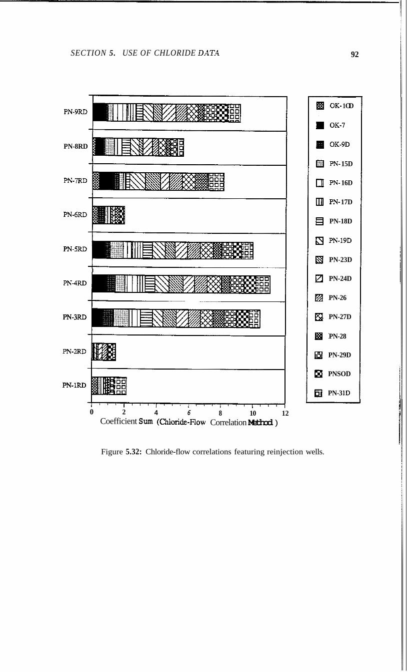
SECTION 5. USE OF CHLORIDE DAT4 92
I
PN-9RD
PN-8RD
PN-7RD
PN-6RD
PN-SRD
I I
PN-4RD
PN-2RD
0 2 Coefficient Sum
4 6 (Chloride-Flow
8 10 12 Correlation Method )
OK- 1 OD
0k-7
0k-9d
PN- 15D
PN- 16D
PN- 17D
PN-18D
PN- 19D
PN-23D
PN-24D
PN-26
PN-27D
PN-28
PN-29D
PNSOD
PN-3 1D
Figure 5.32: Chloride-flow correlations featuring reinjection wells.
SECTION 5. USE OF CHLORIDE DATA 93
them as PN-4RD, PN-3RD, PN-5RD, and PN-8RD, while the last in the
hierarchy to do damage are PN-GRD, PN-lRD, and PN-2RD. From pre-
vious discussions on chloride-flow correlation method, it was put forward
that the reason for the high correlation coefficients of PN-SRD, PN-4RD, PN-5RD, PN-8RD was the continuous utilization of these wells during the
time interval. The results of the linear combination method, on the other hand, do not show such dependence on the injection well utilization since
PN-4RD, PN-5RD, and PN-6RD have much lower correlations compared
to PN-3RD:It will be reiterated that the wells ranked with no or minimal
communication to the producing sectors are PN-2RD, PN-SRD, PN-4RD,
and PN-5RD and the wells proven "deleterious" are PN-SRD, PN-8RD, PN-7RD, PN-lRD, and PN-6RD. Therefore, it can be seen that the linear combination method approaches that of the field experience results.
To conclude, this section shows that the linear combination method is more sensitive to the producer/injector relationship. Therefore, the coefficients of correlation between injector/producer pairs can be used as inputs in the algo- rithms to optimize the production and injection strategy of the geothermal field under exploitation.
5.4.2 Using the Linear Combination Method in More Detail
The linear combination method may be used to investigate in more detail the relationships of the injection wells with the producers. By using appropriate time intervals where different sets of injection wells are used, the method can be used to define more clearly the contributions of the injection wells to the producing well.
As an example, Table 5.8 shows some runs on OK-7 for different time intervals
with different reinjection wells being active during these times. Run No. 1 uses
the whole data set for all wells. The result shows PN-9RD and PN-3RD with
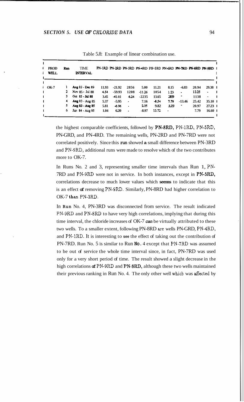
SECTION 5. USE OF CHLORTDE DATA 94
Table 5.8: Example of linear combination use.
I I
I W E L L m v A L I I I I 1
I 2 NOV 85 - JuI 88 454 -59.93 1208 -11.26 1054 1.23 - 13.25 - I I 3 Oa 85 -Jpl88 3.45 43.81 6.24 -2235 13.65 269 - 1138 - I I 4 AUg 8 3 - M 85 5.37 -5.95 - 7.16 -854 7.79 -13.46 25.42 35.10 I I 5 -83-Ang85 5.81 4% - 205 9.82 1.23 - 20.97 27.23 I I 6 Jun84-Aug85 1.04 6.20 - -8.97 13.72 - 7.79 16.60 I I I
1 PROD Rnn TIME PN-1RD PN-2RD PN-3RD PN4RD PN-SRD PNQU) PN-7RD PN-8RD PN-9RD I
1 OK-7 1 @ 83-Dec89 11.93 -21.92 2856 5.00 11.21 8.15 -6.83 20.94 29.38 I
the highest comparable coefficients, followed by PN-8RD, PN-lRD, PN-SRD, PN-GRD, and PN-4RD. The remaining wells, PN-2RD and PN-7RD were not correlated positively. Since this run showed a small difference between PN-3RD and PN-SRD, additional runs were made to resolve which of the two contributes more to OK-7.
In Runs No. 2 and 3, representing smaller time intervals than Run 1, PN- 7RD and PN-9RD were not in service. In both instances, except in PN-5RD, correlations decrease to much lower values which seems to indicate that this
is an effect of removing PN-9RD. Similarly, PN-8RD had higher correlation to
OK-7 than PN-3RD.
In Run No. 4, PN-3RD was disconnected from service. The result indicated PN-9RD and PN-8RD to have very high correlations, implying that during this
time interval, the chloride increases of OK-7 can be virtually attributed to these
two wells. To a smaller extent, following PN-8RD are wells PN-GRD, PN-4RD, and PN-1RD. It is interesting to see the effect of taking out the contribution of PN-7RD. Run No. 5 is similar to Run No. 4 except that PN-7RD was assumed
to be out of service the whole time interval since, in fact, PN-7RD was used
only for a very short period of time. The result showed a slight decrease in the high correlations of PN-9RD and PN-8RD, although these two wells maintained their previous ranking in Run No. 4. The only other well whicb was affected by

SECTION 5. USE OF CHLORIDE DATA 95
this hypothetical run was PN-5RD whose correlation switched from a negative
to a positive value.
For the last run (Run No. 6), wells PN-3RD, PN-6RD and PN-7RD were not employed. Again, the results showed highest coefficients for PN-SRD, followed
by PN-5RD and PN-8RD.
In summary, while the whole data set tends to purport that PN-3RD and PN-
9RD as almost equal in contribution to producer OK-7, the subsets or actual
runs for different time intervals prove that PN-9RD actually has a much greater
weight. It also shows that PN-8RD comes in second, followed by PN-3RD, PN- 5RD, PN-GRD, and PN-1RD.
This illustrates simply how the linear combination method can be used to inves-
tigate, by the process of deduction, the different roles played by the reinjection
wells to the producing wells. In this manner, it can serve as another tool for the efficient management of the reservoir by identifying "fast" reinjection paths.

Section 6
Conclusions and
Recommendation
1. The Palinpinon-I tracer tests results, along with field geometry and well/field
operating constraints were successfully used as input to the algorithms de- veloped and modified by James Lovekin to allocate production and rein-
jection rates to the Palinpinon-I wells. The algorithms employing linear
and quadratic programming allocated the same rates to the wells and cur- tailed the wells one by one partially, then completely, depending on the propensity for thermal breakthrough as indicated by the producer/injector cost coefficient.
2. Due to economic and operational constraints imposed by tracer tests, there
was a need to look for another parameter that can replace tracer data co- efficients in the optimization algorithms. The chloride value was used because it was good indicator of the magnitude and strength of the rela- tionship between the injector and the producer. Four different methods were employed to obtain the correlation between a producer and an injec- tor.
3. One method obtained the correlation between the chloride value and the cumulative flowrate of the injection well. The method, however, had to be
96

SECTION 6. CONCLUSIONS AND RECOMMENDATION 97
disregarded because it tended to give positive high coefficients throughout
the time interval and did not differentiate sufficiently correlation among
the reinjection wells.
4. Another method obtained the correlation between the deviation of chloride from the best fit line to the chloride trend and the injection flowrate of the well. This method was better than the first but had to be discarded because
it produced results contrary to the tracer return data.
5. The third method which determined the correlation between the chloride value and the injection flowrate approaches the tracer test results. It can
be used to rank production wells for each reinjection well, but fails to
separate or distinguish the contributions of the different injection wells
for a particular production well. It also displayed greater sensitivity or dependency on the utilization of the injection well.
6. This deficiency is overcome by the linear combination method which ex- presses the chloride value as a linear combination of the injection wells active during the time interval considered. As such, the weights of the in-
jection wells are taken into account. The result showed that the ranking of
the reinjection wells according to the propensity for communication with
the producing sector is very close to that determined from field observation.
It is, however, different in ranking PN-3RD first.
7. The linear combination method can also rank production wells affected by reinjection returns. The results verify that PN-29D is most severely affected and imply that PN-24D, PN-18D, and PN-27D are three other
wells greatly affected by reinjection returns.
8. The coefficient of correlation between producer/injector pair calculated from the linear combination method can be used as arc cost coefficients to optimize the well utilization strategy. However, this is useful only when
the geothermal field still has the flexibility to utilize and manipulate the
appropriate wells.
9. The Palinpinon Geothermal Field has a wealth of production and chemical

I
SECTION 6. CONCLUSIONS AND RECOMMENDATION 98
data which are usually functions of time. It is recommended that these
data undergo analysis for time series modeling and forecasting which may
be used for reservoir simulation and field management.

Appendix A
Production and Injection Zones
of Paln-I Wells
99
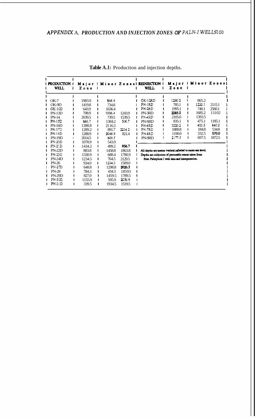
APPENDlX A. PRODUCTION AND INJECTION ZONES OF PALN-I WELLS100
Table A.l: Production and injection depths.
I I I I I I OK-7 I 1983.9 I I OK-9D I 1419.8 I I OK-1OD I 643.9 I I PN-13D I 708.9 I PN-14 I 2039.5 I PN-ISD I 886.7 I PN-16D I 1388.8 I PN-17D I 1289.2 I PN-18D I 1288.9 I PN-19D 1 2014.5 I PN-2OD I PN-2lD I PN-22D I PN-23D I PN-24D I PN-26 I PN-27D I PN-28 I PN-29D I PN3OD I PN31D
I I I I I I I I I I I
1078.9 1434.2 883.8
1330.9 1234.5 934.0 648.8 784.3 827.0
1155.9 339.5
I I I I I I I I I I I I 1 I I I I I
1 I I I 868.9 I OK-1zRD I 12802 1 865.2 I 734.8 I PN-1RD I 785.1 I 1220.1 2115.1
1636.4 I PN-2RD I 1995.1 I 740.1 2560.1 1006.4 1243.9 I PN-3RD 739.5 1539.5 I PN-4RD
21 16.3 I PN4RD 891.7 2234.2 I PN-7F3
2048.9 821.4 I PN-8RD 609.5 I PN-9RD
1384.2 506.7 I PN-SRD
22852 I 1685.2 13102 2105.0 1 1393.5 835.1 I 475.1 1185.1
1220.2 I 420.2 8402 1889.8 I 184.8 534.8 1190.0 I 332.5 570.0 2177.5 I 697.5 1872.5
543.9 499.2
1458.8 688.4 764.5
1234.0 1298.8 434.3
1459.5 595.9
1934.5
956.7 1863.8 1780.9 2129.5 1509.0
18593 1789.5
1519.5
20x3
2050.9
Appendix B
Sample Output from Linear Programming
101
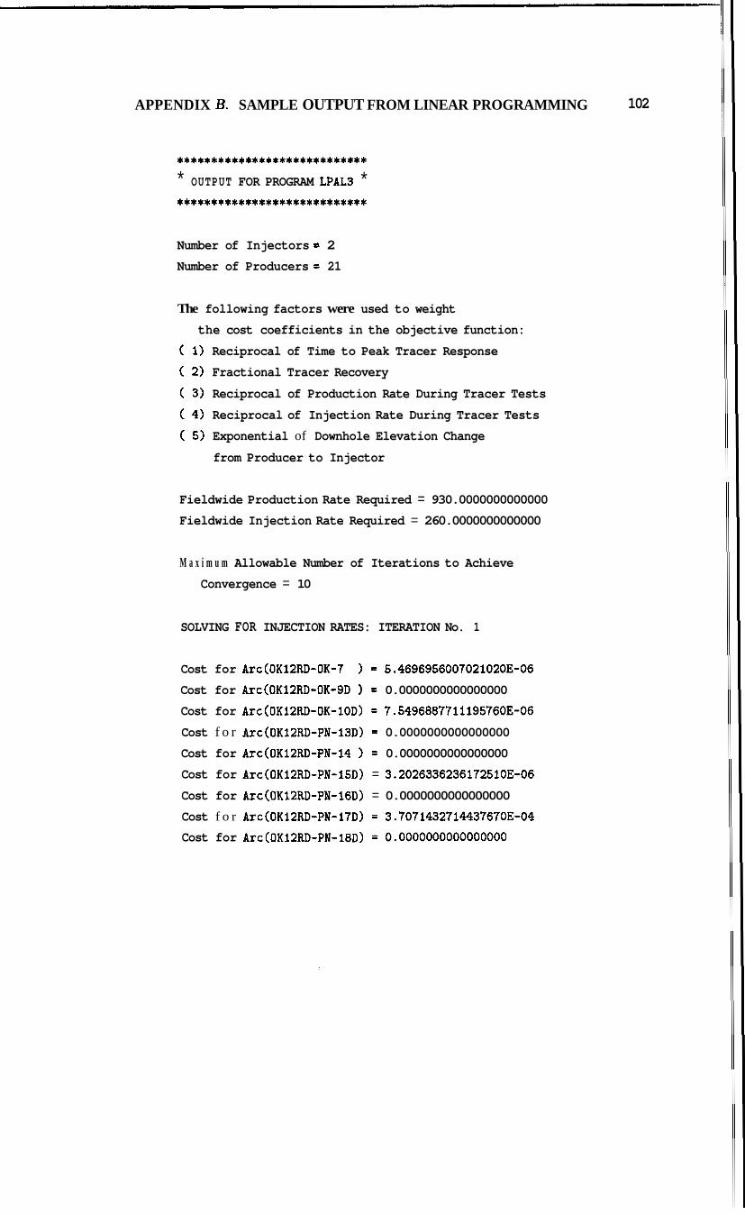
APPENDIX B. SAMPLE OUTPUT FROM LINEAR PROGRAMMING 102
. . . . . . . . . . . . . . . . . . . . . . . . . . . . * OUTPUT FOR PROGRAM LPALB * . . . . . . . . . . . . . . . . . . . . . . . . . . . .
Number of Injectors = 2 Number of Producers = 21
The following factors were used to weight the cost coefficients in the objective function:
( 1) Reciprocal of Time to Peak Tracer Response ( 2) Fractional Tracer Recovery
( 3) Reciprocal of Production Rate During Tracer Tests
( 4) Reciprocal of Injection Rate During Tracer Tests ( 5) Exponential of Downhole Elevation Change
from Producer to Injector
Fieldwide Production Rate Required = 930.0000000000000 Fieldwide Injection Rate Required = 260.0000000000000
M a x i m u m Allowable Number of Iterations to Achieve Convergence = 10
SOLVING FOR INJECTION RATES: ITERATION No. 1
Cost for Arc(OKl2RD-OK-7 = 5.4696956007021020E-06 Cost for Arc(OKl2RD-OK-SD = 0.0000000000000000 Cost for Arc(OKl2RD-OK-1OD) = 7.5496887711195760E-06
Cost f o r Arc(OKl2RD-PN-13D) = 0.0000000000000000 Cost for Arc(OK12RD-PN-14 = 0.0000000000000000 Cost for Arc(OK12RD-PN-15D) = 3.2026336236172510E-06
Cost for Arc(OKl2RD-PN-16D) = 0.0000000000000000 Cost f o r Arc(OK12RD-PN-17D) = 3.7071432714437670E-04 Cost for Arc(OKl2RD-PN-18D) = 0.0000000000~00000
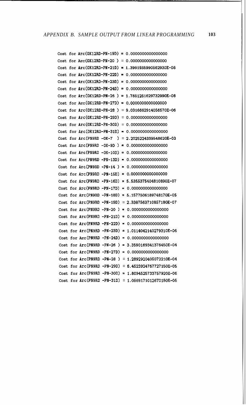
APPENDIX B. SAMPLE OUTPUT FROM LINEAR PROGRAMMING
Cost for Arc(OKl2RD-PN-19D) = 0.0000000000000000 Cost for Arc (OKl2RD-PN-20 ) = 0.0000000000000000 Cost for Arc(OK12RD-PN-2lD) = 1.3991935990562930E-08 Cost for Arc(OKl2RD-PN-22D) = 0.0000000000000000 Cost for Arc(OKl2RD-PN-23D) = 0.0000000000000000 Cost for Arc(OKl2RD-PN-24D) = 0.0000000000000000
Cost for Arc(OKl2RD-PN-26 = 1.7851251629732990E-08 Cost for Arc (OK12RD-PN-27D) = 0 .OOOOOOOOOOOOOOOO Cost for Arc(OK12RD-PN-28 ) = 9.0316662914056570E-06
Cost for Arc(OKlZRD-PN-29D) = 0.0000000000000000 Cost for Arc(OKl2RD-PN-30D) = 0.0000000000000000
Cost for Arc(OKl2RD-PN-3lD) = 0.0000000000000000 Cost for Arc(PN9RD -0K-7 ) = 2.2025224339548620E-03
Cost for Arc(PN9RD -0K-9D = 0.0000000000000000 Cost for Arc(PN9RD -0K-1OD) = 0.0000000000000000 Cost for Arc(PN9RD -PN-l3D) = 0.0000000000000000
Cost for Arc(PN9RD -PI-14 ) = 0.0000000000000000 Cost for Arc(PN9RD -PN-l5D) = 0 .OOOOOOOOOOOOOOOO Cost for Arc(PN9RD -PN-l6D) = 5.5355375404810890E-07 Cost for Arc(PN9RD -PN-l7D) = 0.0000000000000000 Cost for Arc(PN9RD -PN-l8D) = 5.1577506189748170E-05 Cost for Arc(PN9RD -PN-l9D) = 2.3387563710857180E-07
Cost for Arc(PN9RD -PN-20 = 0.0000000000000000 Cost for Arc(PN9RD -PN-21D) = 0.0000000000000000 Cost for Arc(PN9RD -PN-22D) = 0.0000000000000000
Cost for Arc(PN9RD -PN-23D) = 1.0114042140279310E-06 Cost for Arc (PN9RD -PN-24D) = 0.0000000000000000 Cost for Arc(PN9RD -PN-26 ) = 3.3590169341376450E-04 Cost for Arc(PN9RD -PN-27D) = 0.0000000000000000 Cost for Arc(PN9RD -PN-28 ) = 1.2892920405072210E-04 Cost for Arc(PN9RD -PN-29D) = 6.4523924767727150E-05 Cost for Arc(PN9RD -PN-BOD) = 1.8094525733757920E-06 Cost for Arc(PN9RD -PN-31D) = 1.0569171012670150E-05
103
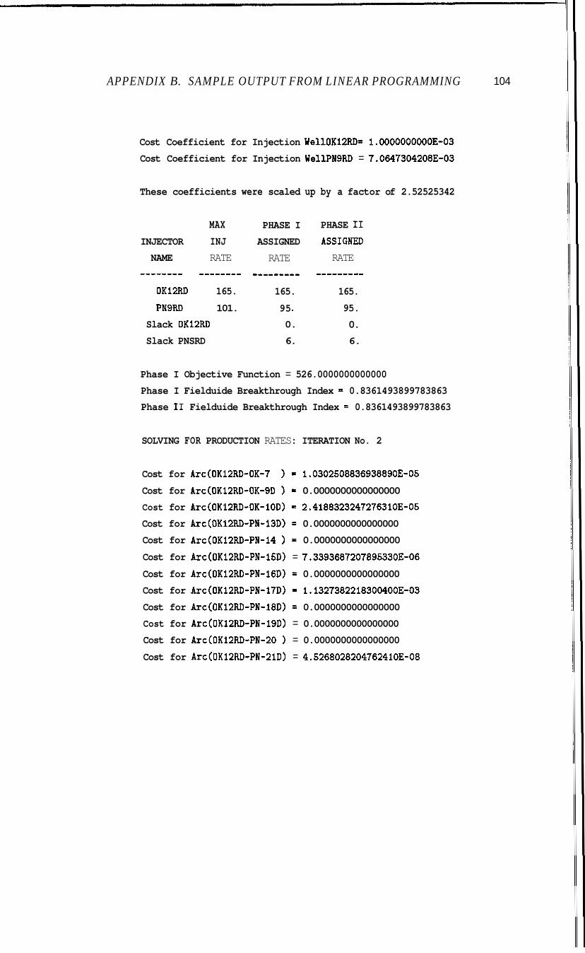
APPENDIX B. SAMPLE OUTPUT FROM LINEAR PROGRAMMING 104
Cost Coefficient for Injection WellOKl2RD= 1.0000000000E-03 Cost Coefficient for Injection WellPNSRD = 7.0647304208E-03
These coefficients were scaled up by a factor of 2.52525342
MAX PHASE I INJECTOR INJ ASSIGNED NAME RATE RATE
-------- -------- --------- OK12RD 165. 165.
PNSRD 101. 95 * Slack OKl2RD 0.
Slack PNSRD 6.
PHASE I1 ASSIGNEX) RATE
--------- 165.
95. 0. 6.
Phase I Objective Function = 526.0000000000000 Phase I Fielduide Breakthrough Index = 0.8361493899783863 Phase I1 Fielduide Breakthrough Index = 0.8361493899783863
SOLVING FOR PRODUCTION RATES: ITERATION No. 2
Cost for Arc(OK12RD-OK-7 = 1.0302508836938890E-05 Cost for Arc(OKl2RD-OK-9D ) = 0.0000000000000000 Cost for Arc(OKl2RD-OK-1OD) = 2.4188323247276310E-05 Cost for Arc(OK12RD-PN-13D) = 0.0000000000000000 Cost for Arc(OK12RD-PN-14 ) = 0.0000000000000000 Cost for Arc(OKl2RD-PN-15D) = 7.3393687207895330E-06
Cost for Arc(OKl2RD-PN-16D) = 0.0000000000000000 Cost for Arc(OK12RD-PN-17D) = 1.1327382218300400E-03
Cost for Arc(OK12RD-PN-18D) = 0.0000000000000000 Cost for Arc(OKl2RD-PN-19D) = 0.0000000000000000 Cost for Arc(OK12RD-PN-20 ) = 0.0000000000000000
Cost for Arc(OKl2RD-PN-2lD) = 4.5268028204762410E-08
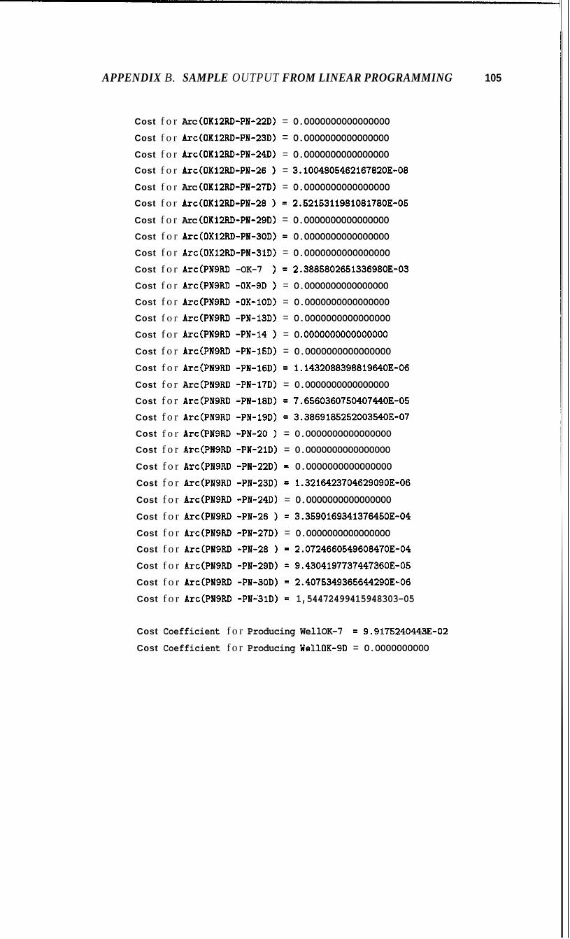
APPENDIX B. SAMPLE OUTPUT FROM LINEAR PROGRAMMING 105
Cost f o r Arc (OK12RD-PN-22D) = 0.0000000000000000
Cost f o r Arc(OKl2RD-PN-23D) = 0.0000000000000000 Cost f o r Arc(OK12RD-PN-24D) = 0.0000000000000000 Cost f o r Arc(OK12RD-PN-26 = 3.1004805462167820E-08
Cost f o r Arc (OKl2RD-PN-27D) = 0.0000000000000000 Cost f o r Arc(OK12RD-PN-28 ) = 2.5215311981081780E-05 Cost f o r Arc (OKl2RD-PN-29D) = 0.0000000000000000 Cost f o r Arc(OKl2RD-PN-30D) = 0.0000000000000000 Cost f o r Arc(OK12RD-PN-3lD) = 0.0000000000000000 Cost f o r Arc(PN9RD -OK-7 = 2.3885802651336980E-03 Cost f o r Arc(PN9RD -OK-9D 1 = 0.0000000000000000 Cost f o r Arc(PN9RD -OK-1OD) = 0.0000000000000000 Cost f o r Arc(PN9RD -PN-l3D) = 0.0000000000000000 Cost f o r Arc(PN9RD -PN-14 ) = 0 .OOOOOOOOOOOOOOOO Cost f o r Arc(PN9RD -PN-l5D) = 0.0000000000000000 Cost f o r Arc(PN9RD -PN-lGD) = 1.1432088398819640E-06 Cost f o r Arc (PN9RD -PN-l7D) = 0.0000000000000000 Cost f o r Arc(PN9RD -PN-l8D) = 7.6560360750407440E-05 Cost f o r Arc(PN9RD -PN-lSD) = 3.3869185252003540E-07 Cost f o r Arc(PN9RD -PN-20 ) = 0.0000000000000000 Cost f o r Arc(PN9RD -PN-2lD) = 0.0000000000000000
Cost f o r Arc(PN9RD -PN-22D) = 0.0000000000000000 Cost f o r Arc(PN9RD -PN-23D) = 1.3216423704629090E-06 Cost f o r Arc(PN9RD -PN-24D) = 0.0000000000000000
Cost f o r Arc(PN9RD -PI-26 = 3.3590169341376450E-04 Cost f o r Arc(PN9RD -PN-27D) = 0.0000000000000000 Cost f o r Arc(PN9RD -PN-28 = 2.0724660549608470E-04
Cost f o r Arc(PN9RD -PN-29D) = 9.4304197737447360E-05 Cost f o r Arc(PN9RD -PN-30D) = 2.4075349365644290E-06
Cost f o r Arc(PN9RD -PN-'31D) = 1,54472499415948303-05
Cost Coefficient f o r Producing WellOK-7 = 9.9175240443E-02 Cost Coefficient f o r Producing WellOK-9D = 0.0000000000
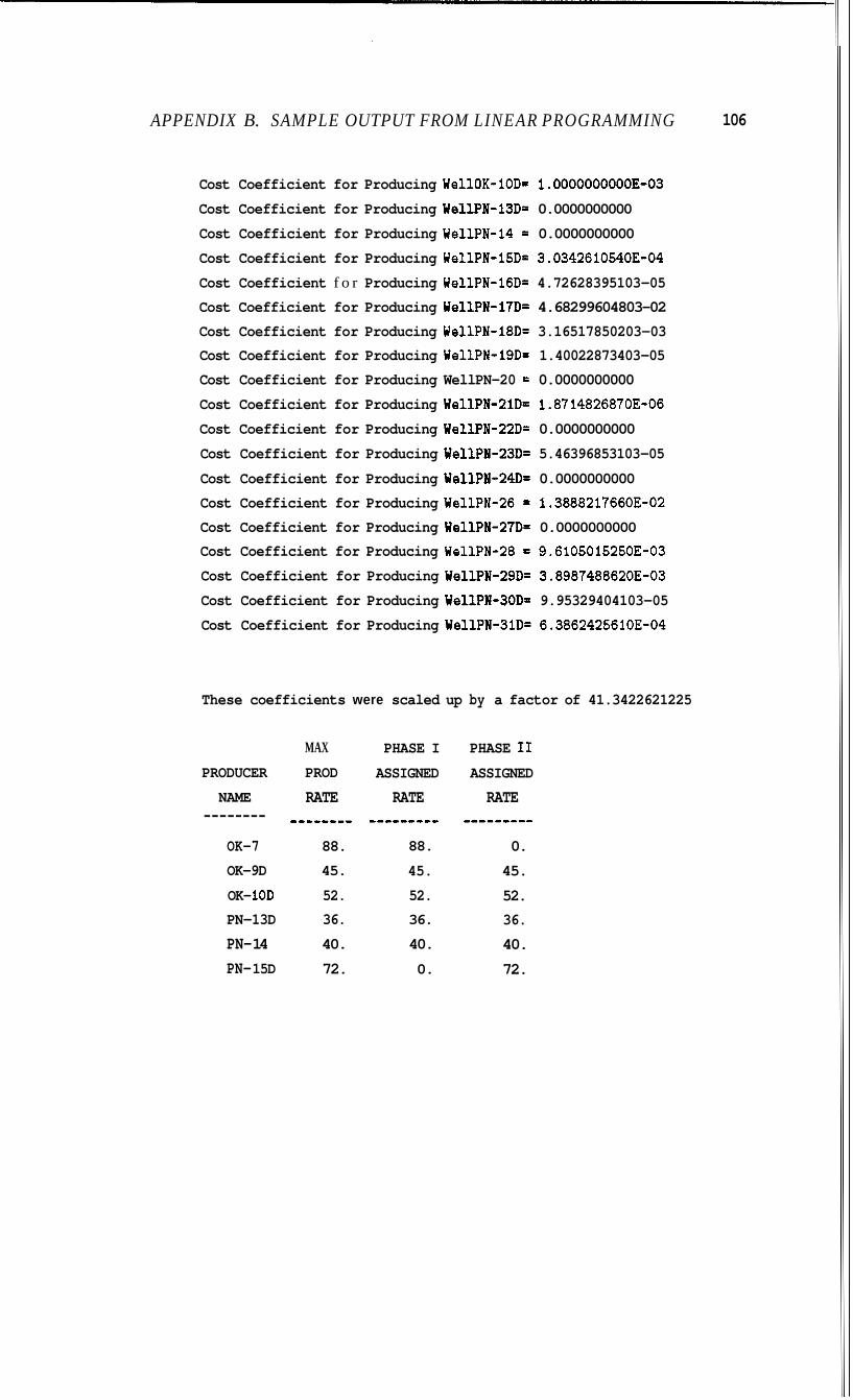
APPENDIX B. SAMPLE OUTPUT FROM LINEAR PROGRAMMING
Cost Coefficient for Producing WellOK-lOD= 1.0000000000E-03
Cost Coefficient for Producing WellPN-l3D= 0.0000000000
Cost Coefficient for Producing WellPN-14 = 0.0000000000 Cost Coefficient for Producing WellPN-l5D= 3.0342610540E-04 Cost Coefficient f o r Producing WellPN-16D= 4.72628395103-05 Cost Coefficient for Producing WellPN-l7D= 4.68299604803-02 Cost Coefficient for Producing WellPN-l8D= 3.16517850203-03 Cost Coefficient for Producing WellPN-19D= 1.40022873403-05 Cost Coefficient for Producing WellPN-20 = 0.0000000000 Cost Coefficient for Producing WellPN-2lD= 1.8714826870E-06
Cost Coefficient for Producing WellPN-22D= 0.0000000000
Cost Coefficient for Producing WellPN-23D= 5.46396853103-05
Cost Coefficient for Producing WellPN-24D= 0.0000000000 Cost Coefficient for Producing WellPN-26 = 1.3888217660E-02 Cost Coefficient for Producing WellPN-27D= 0.0000000000 Cost Coefficient for Producing WellPN-28 = 9.6105015250E-03
Cost Coefficient for Producing WellPN-29D= 3.8987488620E-03
Cost Coefficient for Producing WellPN-30D= 9.95329404103-05
Cost Coefficient for Producing WellPN-31D= 6.3862425610E-04
These coefficients were scaled up by a factor of 41.3422621225
106
PRODUCER
NAME --------
OK-7 OK-9D
OK- 1OD PN-13D
PN- 14 PN- 15D
MAX
PROD
RATE --------
88. 45.
52. 36.
40.
72.
PHASE I
ASSIGNED
RATE ---------
88.
45.
52. 36.
40.
0.
PHASE I1
ASSIGNED
RATE ---------
0.
45.
52. 36.
40.
72.
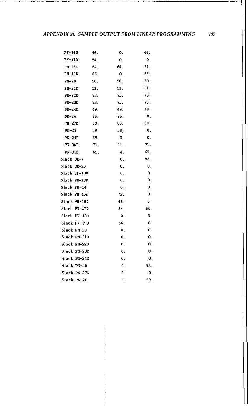
APPENDIX 33. SAMPLE OUTPUT FROM LINEAR PROGRAMMING 107
PN-16D 46.
PN-17D 54. PN-18D 64.
PN- 19D 66.
PN-20 50.
PN-21D 51.
PN-22D 73. PN-23D 73. PN-24D 49. PN-26 95. PI-27D 80.
PN-28 59.
PN-29D 65.
PN-BOD 71. PN-31D 65.
Slack OK-7 Slack OK-9D Slack OK-1OD Slack PN-13D Slack PN-14 Slack PN-15D
Slack PN-16D Slack PN-17D
Slack PN- 18D Slack PN-19D Slack PN-20 Slack PN-21D
Slack PN-22D Slack PN-23D
Slack PN-24D
Slack PN-26
Slack PN-27D
Slack PN-28
0.
0.
64.
0.
50.
51.
73. 73. 49. 95. 80.
59,
0.
71.
4. 0.
0.
0.
0.
0.
72.
46.
54. 0.
66. 0.
0.
0.
0.
0.
0.
0.
0.
46.
0. 61.
66.
50.
51.
73. 73. 49. 0.
80.
0.
0.
71. 65. 88.
0.
0.
0.
0.
0.
0. 54.
3.
0.
0.
0.
0.
0.
0.
95.
0.
59.
APPENDIX B. SAMPLE OUTPUT FROM LINEAR PROGRAMMING 108
Slack PN-29D
Slack PN-SOD Slack PN-BID
65. 65.
0. 0. 61. 0.
Phase I Objective Function = 2223.400000000000 Phase I Fieldvide Breakthrough Index = 10.84304042994569
Phase I1 Fieldwide Breakthrough Index = 0.3231497417919218
SOLVING FOR INJECTION RATES: ITERATION No. 3
Cost for Arc(OK12RD-OK-7 ) = 0.0000000000000000 Cost for Arc(OKl2RD-OK-9D ) = 0.0000000000000000 Cost for Arc(OKl2RD-OK-1OD) = 7.5496887711195760E-06 Cost for Arc(OKl2RD-PN-13D) = 0.0000000000000000
Cost for Arc(OK12RD-PN-14 = 0.0000000000000000 Cost for Arc(OK12RD-PN-15D) = 3.2026336236172510E-06
Cost for Arc(OK12RD-PN-16D) = 0.0000000000000000
Cost for Arc(OK12RD-PN-17D) = 0.0000000000000000 Cost f o r Arc(OKl2RD-PN-18D) = 0.0000000000000000
Cost f o r Arc(OK12RD-PN-19D) = 0.0000000000000000 Cost for Arc(OKl2RD-PN-20 ) = 0.0000000000000000
Cost for Arc(OK12RD-PN-2lD) = 1.3991935990562930E-08 Cost for Arc(OK12RD-PN-22D) = 0.0000000000000000 Cost for Arc(OKl2RD-PN-23D) = 0.0000000000000000
Cost for Arc(OK12RD-PN-24D) = 0.0000000000000000 Cost for Arc (OK12RD-PN-26 = 0.0000000000000000 Cost for Arc(OK12RD-PN-27D) = 0.0000000000000000 Cost for Arc(OK12RD-PN-28 ) = 0.0000000000000000 Cost for Arc(OK12RD-PN-29D) = 0.0000000000000000
Cost for Arc(OK12RD-PN-30D) = 0.0000000000000000 Cost for Arc (OK12RD-PN-3lD) = 0.0000000000000000 Cost for Arc(PN9RD -0K-7 ) = 0.0000000000000000 Cost for Arc(PN9RD -0K-9D ) = 0.0000000000000000
APPENDIX B. SAMPLE OUTPUT FROM LINEAR PROGRAMMING
Cost for Arc(PN9RD -OK-1OD) = 0.0000000000000000 Cost for Arc(PN9RD -PN-l3D) = 0.0000000000000000
Cost for Arc(PN9RD -PN-14 ) = 0.0000000000000000 Cost for Arc(PN9RD -PN-l5D) = 0.0000000000000000
Cost for Arc(PN9RD -PN-l6D) = 5.5355375404810890E-07 Cost for Arc(PN9RD -PN-l7D) = 0.0000000000000000 Cost for Arc(PN9RD -PN-l8D) = 4.9401580147368130E-05 Cost for Arc(PN9RD -PN-l9D) = 2.3387563710857180E-07 Cost for Arc(PN9RD -PN-20 = 0.0000000000000000
Cost for Arc(PN9RD -PN-21D) = 0.0000000000000000 Cost for Arc (PN9RD -PN-22D) = 0.0000000000000000
Cost for Arc(PN9RD -PN-23D) = 1.0114042140279310E-06 Cost for Arc(PN9RD -PN-24D) = 0.0000000000000000 Cost for Arc(PN9RD -PN-26 = 0.0000000000000000
Cost for Arc(PN9RD -PN-27D) = 0.0000000000000000 Cost for Arc(PN9RD -PN-28 ) = 0.0000000000000000 Cost for Arc(PN9RD -PN-29D) = 0.0000000000000000 Cost for Arc(PN9RD -PN-BOD) = 1.8094525733757920E-06
Cost for Arc(PN9RD -PN-3lD) = 1.0569171012670150E-05
Cost Coefficient for Injection WellOKl2RD= 1.0000000000E-03
Cost Coefficient for Injection WellPN9RD = 5.90536699703-03
These coefficients were scaled up by a factor of 92.882296511
109
MAX INJECTOR IN J NAME RATE
-------- -------- OK12RD 165.
PN9RD 101.
Slack OKl2RD
Slack PN9RD
PHASE I PHASE I1
ASSIGNED ASSIGNED
RATE RATE --------- ---------
165. 165.
95. 95. 0. 0.
6. 6.

APPENDIX 33. SAMPLE OUTPUT FROM LINEAR PROGRAMMING 110
Phase I Objective Function = 526.0000000000000 Phase I Fieldwide Breakthrough Index = 0.7260098648084709 Phase I1 Fieldwide Breakthrough Index = 0.7260098648084709
Convergence Achieved in 3Iterations
Final Assigned Rates are Optimal for Injectors and Producers Fortran STOP
Appendix C
Sample Output from Quadratic
Programming
111
APPENDIX C. SAMPLE OUTPUT FROM QUADRATIC PROGRAMMING 112
. . . . . . . . . . . . . . . . . . . . . . . . . . . . . * OUTPUT FOR PROGRAl4 QPAL * . . . . . . . . . . . . . . . . . . . . . . . . . . . . .
Number of Injectors = 2 Number of Producers = 21
Fieldwide Production Rate Required = 930.0000000000000 Fieldwide Injection Rate Required = 260.0000000000000
The following factors were used in the calculation of arc costs:
( 1) Reciprocal of Time to Peak Tracer Response ( 2) Fractional Tracer Recovery
( 3) Reciprocal of Production Rate During Tracer Tests ( 4) Reciprocal of Injection Rate During Tracer Tests ( 5) Exponential of Downhole Elevation Change
from Producer to Injector
Cost for Arc(OKl2RD-OK-7 ) = 6.2439447496599320E-08 Cost for Arc(OKl2RD-OK-9D ) = 0.0000000000000000 Cost for Arc(OK12RD-OK-1OD) = 1.4659589846834130E-07 Cost for Arc(OK12RD-PN-13D) = 0.0000000000000000 Cost for Arc(OKl2RD-PN-14 ) = 0.0000000000000000 Cost for Arc(OKl2RD-PN-15D) = 4.4481022550239600E-08 Cost for Arc(OK12RD-PN-16D) = 0.0000000000000000 Cost for Arc(OK12RD-PN-17D) = 6.8650801323032700E-06 Cost for Arc(OK12RD-PN-18D) = 0.0000000000000000 Cost for Arc(OKl2RD-PN-19D) = 0.0000000000000000 Cost for Arc(OK12RD-PN-20D) = 0.0000000000000000 Cost for Arc(OK12RD-PN-21D) = 2.7435168608946920E-10 Cost for Arc(OKl2RD-PN-22D) = 0.0000000000000000 Cost for Arc(OK12RD-PN-23D) = 0.0000000000000000
APPENDIX C. SAMPLE OUTPUT FROM QUADRATIC PROGRAMMING 113
Cost for Arc(OK12RD-PN-24D) = 0.0000000000000000 Cost f o r Arc(OKl2RD-PN-26 = 1.8790791189192610E-10 Cost for Arc(OK12RD-PN-27D) = 0.0000000000000000 Cost f o r Arc(OKl2RD-PI-28 = 1.5282007261261690E-07 Cost f o r Arc(OKl2RD-PN-29D) = 0.0000000000000000 Cost f o r Arc(OKl2RD-PN-30D) = 0.0000000000000000 Cost f o r Arc(OK12RD-PN-3lD) = 0.0000000000000000 Cost f o r Arc(PN9RD -OK-7 = 2.5142950159302080E-05 Cost f o r Arc(PN9RD -OK-9D = 0.0000000000000000 Cost f o r Arc(PN9RD -OK-1OD) = 0.0000000000000000 Cost f o r Arc (PN9RD -PI- 13D) = 0.0000000000000000
Cost f o r Arc(PN9RD -PN-14 = 0 .OOOOOOOOOOOOOOOO Cost f o r Arc(PN9RD -PN-l5D) = 0.0000000000000000 Cost f o r Arc(PN9RD -PN-l6D) = 1.2033777261915410E-08
Cost for Arc (PN9RD -PN- 17D) = 0.0000000000000000 Cost f o r Arc(PN9RD -PN-l8D) = 8.0589853421481510E-07 Cost f o r Arc(PN9RD -PN-l9D) = 3.5651773949477410E-09 Cost f o r Arc(PN9RD -PN-20D) = 0.0000000000000000 Cost f o r Arc(PN9RD -PN-2lD) = 0.0000000000000000 Cost f o r Arc(PN9RD -PN-22D) = 0.0000000000000000 Cost f o r Arc(PN9RD -PN-23D) = 1.3912024952241150E-08
Cost f o r Arc(PN9RD -PN-24D) = 0.0000000000000000 Cost for Arc(PN9RD -PN-26 = 3.5358072990922580E-06 Cost for Arc(PN9RD -PN-27D) = 0.0000000000000000 Cost f o r Arc(PN9RD -PI-28 = 2.1815432157482600E-06 Cost for Arc (PN9RD -PN-29D) = 9.9267576565734070E-07 Cost f o r Arc(PN9RD -PN-SOD) = 2.5342473016467680E-08 Cost f o r Arc(PN9RD -PN-31D) = 1.6260263096415610E-07
MAX MIN ASSIGNED INJECTOR INJ IN J IN J
NAME RATE RATE RATE SLACK --------- -------- -------- ---------- --------
OK 12RD 165. 0. 165. 0.
APPENDIX C. SAMPLE OUTPUT FROM QUADRATIC PROGRAMMING 114
PN9RD
PRODUCER NAME
--------- OK-7 OK-9D OK-1OD PN- 13D PN- 14 PN-15D PN-16D PN- 17D PN-18D
PN- 19D
PN-2OD PN-21D
PN-22D
PN-23D PN - 24D PN-26 PN-27D PN-28
PN-29D PN-SOD
PN-31D
101.
HAX PROD RATE
-------- 88. 45. 52.
36.
40.
72. 46. 54.
64. 66.
50.
51.
73.
73. 49.
95.
80. 59.
65.
71.
65.
0.
MIN PROD RATE
-------- 0.
0. 0.
0.
0.
0.
0. 0.
0. 0.
0.
0. 0.
0.
0.
0.
0.
0.
0. 0.
0.
95. 6.
ASSIGNED
PROD RATE SLACK
0.
45. 52.
36.
40.
72. 46. 0.
61.
66.
50. 51.
73.
73. 49.
0.
80.
0.
0.
71. 65.
88.
0.
0.
0.
0.
0.
0.
54.
3.
0.
0.
0.
0.
0.
0.
95. 0.
59.
65.
0.
0.
EXIT QPSOL - OPTIMAL QP SOLUTION.
FINAL VALUE OF FIELDWIDE BREAKTHROUGH INDEX = Fortran STOP
0.7816450E-02
Appendix D
Reservoir Chloride Measurements with Time
115
APPENDIX D. RXSERVOIR CHLORIDE MEASUREMENTS WITH TIME 116
h Q .s
loo00 OK-7 I I I I
8000
7000
6aQ
5000
Moo 1983 1984 1985 1986 1981 1988
-(yur) 1989 1990
Figure D.l: OK-7/OK-9D Reservoir chloride with time.
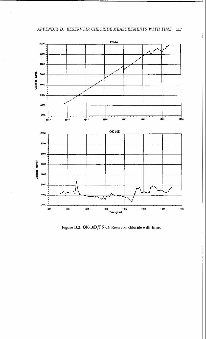
APPENDIX D. RESERVOIR CHLORIDE MEASUREMENTS WITH TIME 117
Figure D.2: OK-lOD/PN-14 Reservoir chloride with time.
-1 1 9!
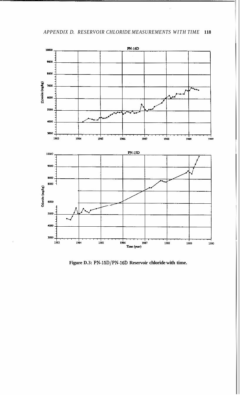
APPENDIX D. RESERVOIR CHLORIDE MEASUREMENTS W I T H TIME 118
P 3 8 a
loo00
-E so00
6OOo
1983 1984
PN-15D
1985 1988 1989 1990
Figure D.3: PN-15D/PN-l6D Reservoir chloride with time.
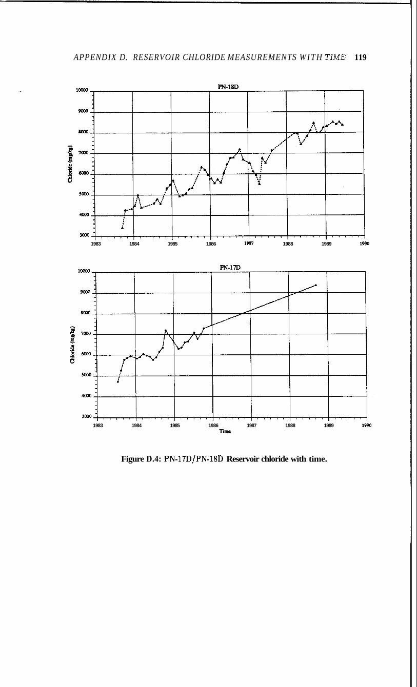
APPENDIX D. RESERVOIR CHLORIDE MEASUREMENTS W I T H T I " 119
1983 1984 1985 1986 1988 1989 1990
1983 1984 1985 1986 1987 1988 1989 1990 T-
Figure D.4: PN-17D/PN-l8D Reservoir chloride with time.
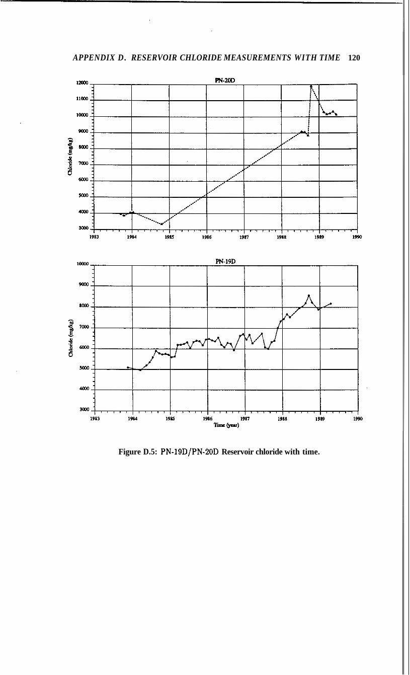
APPENDIX D. RESERVOIR CHLORIDE MEASUREMENTS WITH TIME 120
Figure D.5: PN-lSDIPN-BOD Reservoir chloride with time.
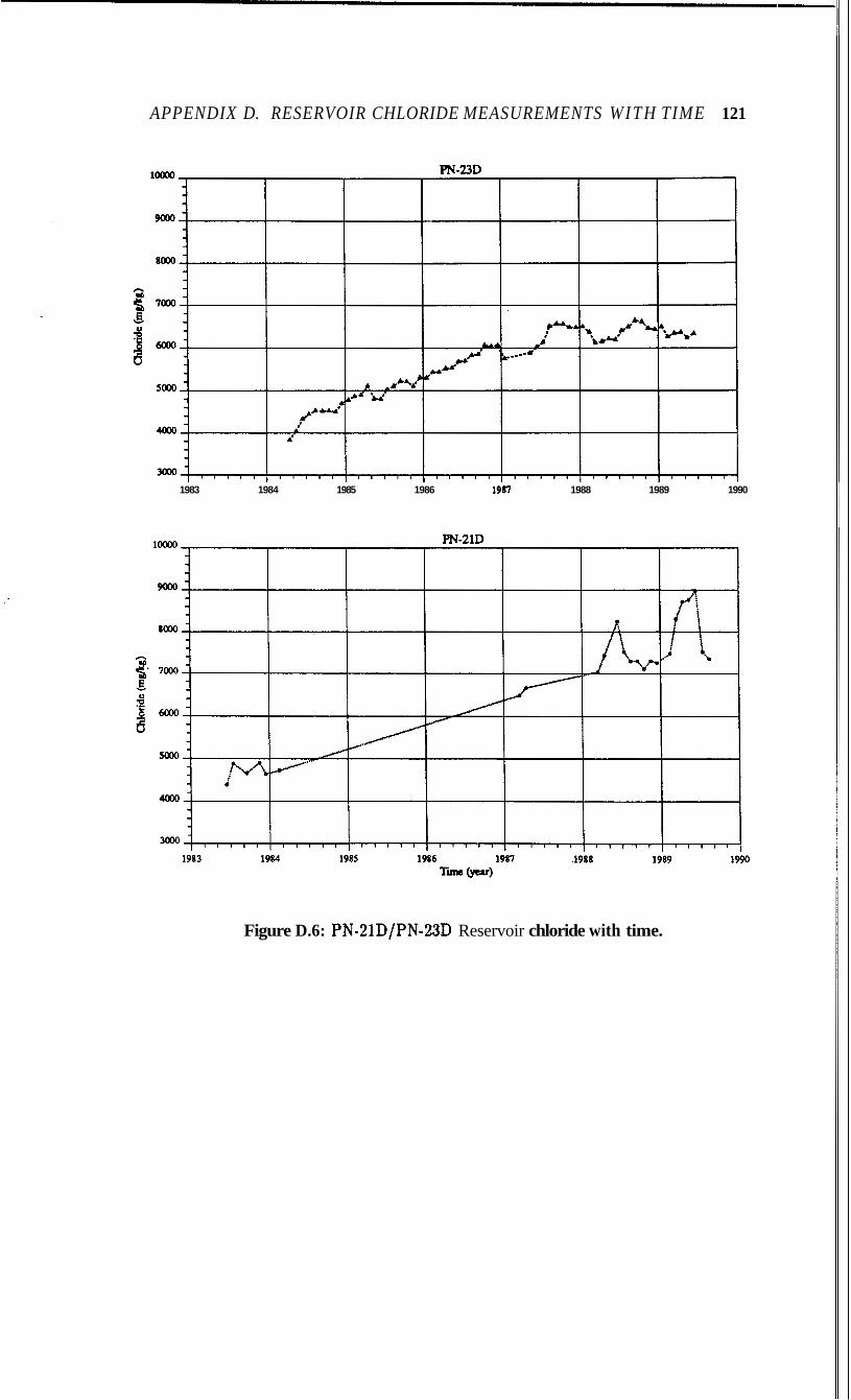
APPENDIX D. RESERVOIR CHLORIDE MEASUREMENTS WITH TIME 121
1983 1984 1985 1986 1988 1989 1990
Figure D.6: PN-21D/PN-23D Reservoir chloride with time.
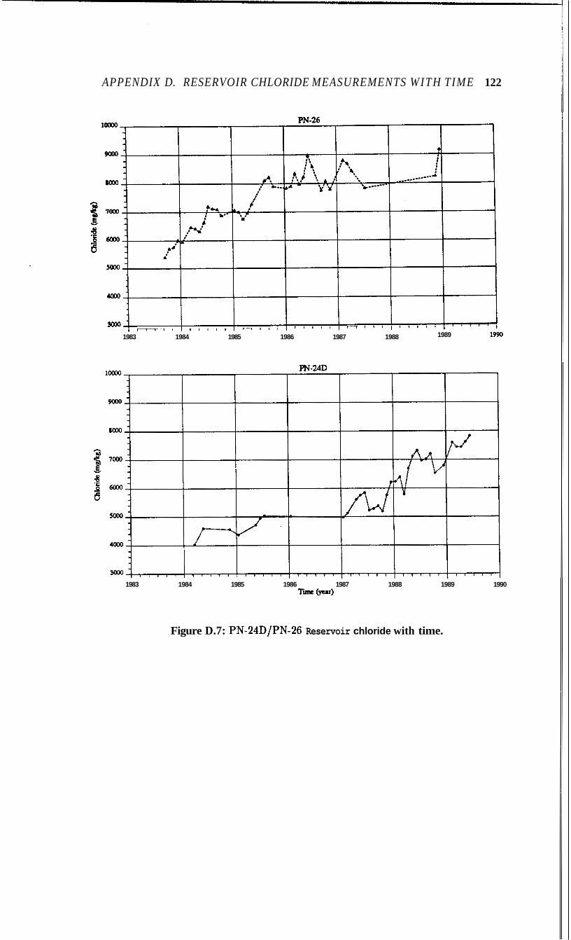
APPENDIX D. RESERVOIR CHLORIDE MEASUREMENTS WITH TIME 122
5000
4ooo
3ooo , , , , , , , , , , , , , , , , , , I , , , I , , I I I I I i i I 1 I
1983 1984 1985 1986 1987 1988 1989 1990
1983 1984 1985 1986 1987 1988 1989 1990 T I W)
Figure D.7: PN-24D/PN-26 Reservoir chloride with time.
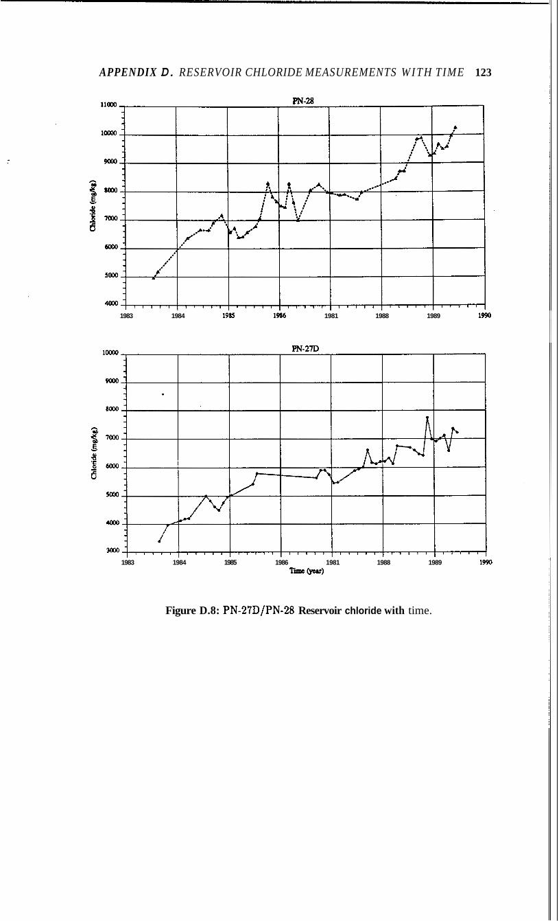
APPENDIX D. RESERVOIR CHLORIDE MEASUREMENTS W I T H TIME 123
1983 1984 1985 1 k 6 1981 1988 1989 1990
1983 1984 1985 1986 1981 1988 1989 1990 T- 6-4
Figure D.8: PN-27D/PN-28 Reservoir chloride with time.
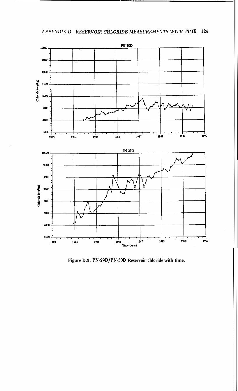
Figure D.9: PN-29D/PN-30D Reservoir chloride with time.
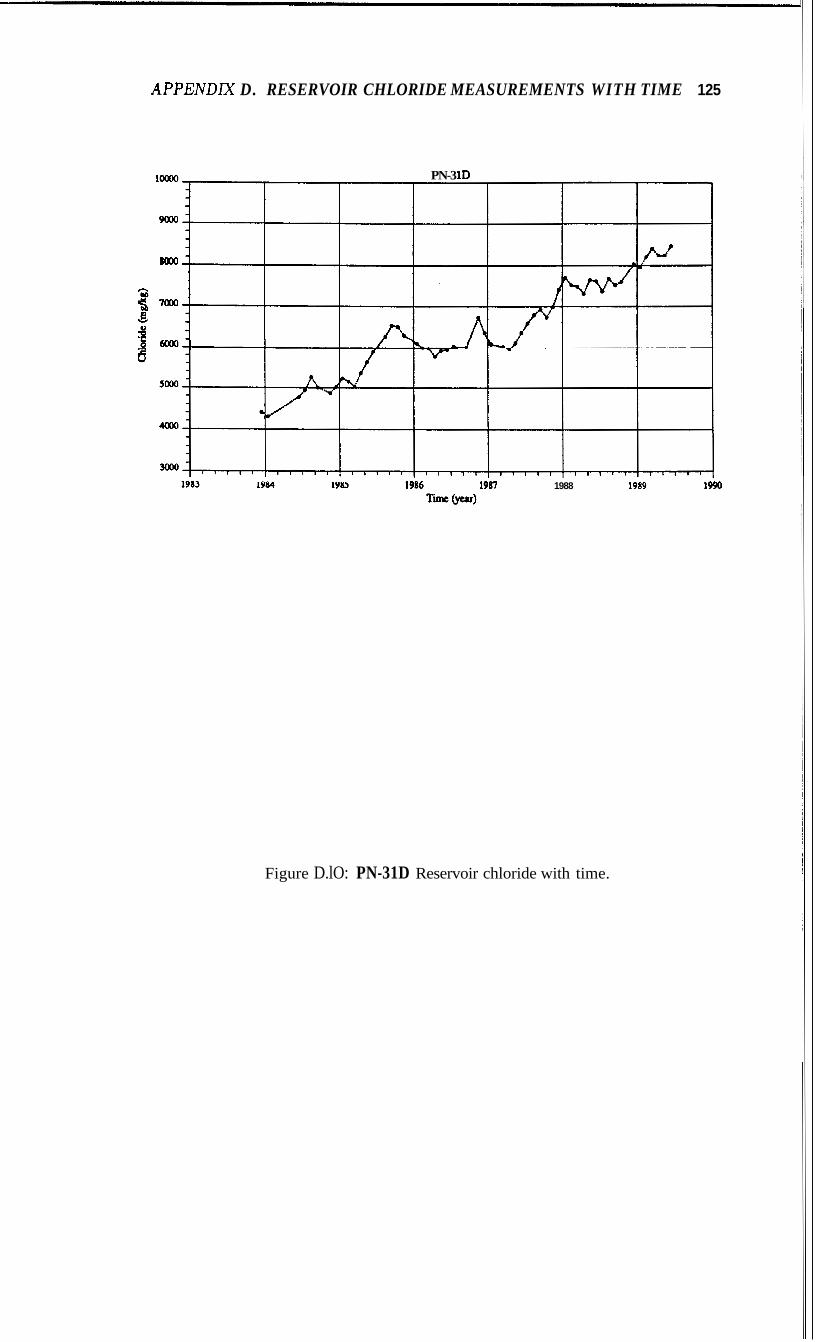
APPENDlX D. RESERVOIR CHLORIDE MEASUREMENTS WITH TIME 125
oooo
Moo
7000
6 o O 0 ,
PN-3 1D ' 1988 1989
Figure D.lO: PN-31D Reservoir chloride with time.
Appendix E
Injection Flowrates with Time
126
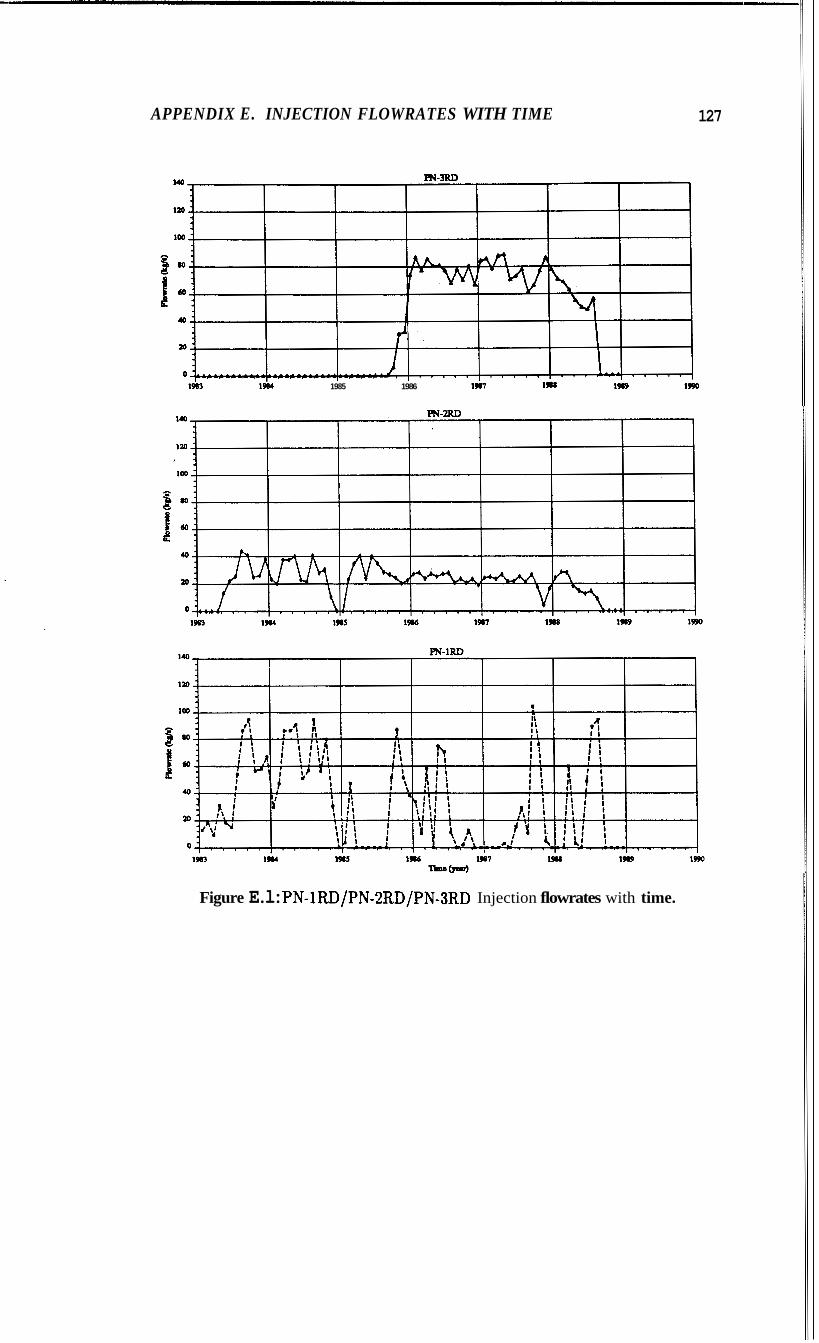
APPENDIX E. INJECTION FLOWRATES WITH TIME 127
1983 1984 1985 1986 1987 1989 1990
Figure E.l: PN-lRD/PN-ZRD/PN-3RD Injection flowrates with time.
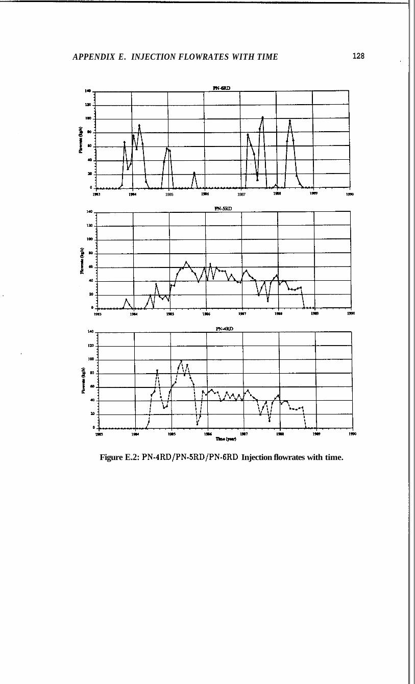
APPENDIX E. INJECTION FLOWRATES WITH TIME 128
1963 1984 1985 1987 1990
Figure E.2: PN-4RD/PN-SRD/PN-GRD Injection flowrates with time.
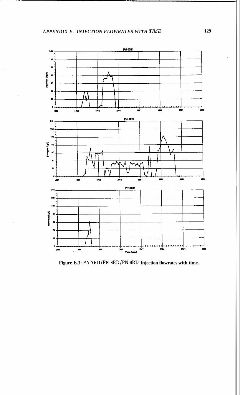
APPENDIX E. INJECTION FLOWRATES WITH TIME 129
0
Figure E.3: PN-7RD/PN-8RD/PN-gRD Injection flowrates with time.

Appendix F
Chloride-Flow Correlations
130
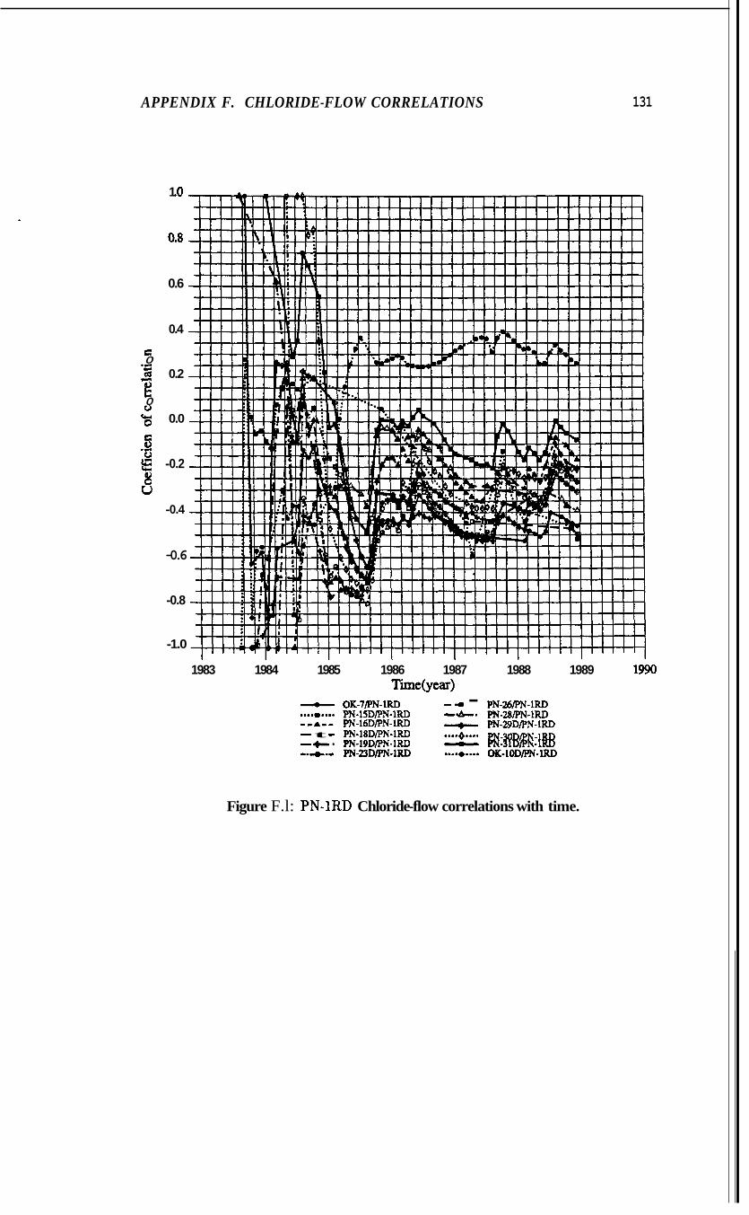
APPENDIX F. CHLORIDE-FLOW CORRELATIONS 131
1 .o
0.8
0.6
0.4
c 0 .m s 0.2
1 0 0
"0 0.0
8 -0.2 5
c .B
u -0.4
-0.6
-0.8
-1.0
1983 1984 1985 1986 1987 1988 1989 1990 Time(year)
OK-7PN-lRD - 4 - PN-%/Fw-lRD *..*o**-* PN-1SDPN-1RD PN-BPN-1RD
+, PN-BDPN-lRD - t PN-18DPN-1RD ....4.... pN-'jODIpN-lRD - C PN-19DPN-1RD --+.- PN-23DPN-lRD & PN-31DPN-1RD ....e.... O K - l O D / p N ~
- -A- - PN-16DPN-lRD
Figure F.l: PN-1RD Chloride-flow correlations with time.

APPENDIX F. CHLORIDE-FLOW CORRELATIONS 132
1.0
0.8
0.6
0.4
8 -4 0.2
“0 0.0
5
8
t 0
c)
.U
-0.2 0
u -0.4
-0.6
-0.8
-1.0
1983 1984 1985 1986 1987 1988 1989 1990 Time(year)
OK-7/PN-2RD - 4 - PN-Zb/PN-m .... om... pN-lSDIpN-2RD -+e PN-28PN-2RD
- t PN-lEDPN-2RD .... 0 .... PN-3ODPN-W * PN-19DPN-2RD - PN-31DPN-2RD
-.IC*- PN-23DPN-2RD ......... OK-lODIpN-ZRD
- - A - - PN-16DPN-2RD PN-29DPN-2RD
Figure F.2: PN-2RD Chloride-flow correlations with time.
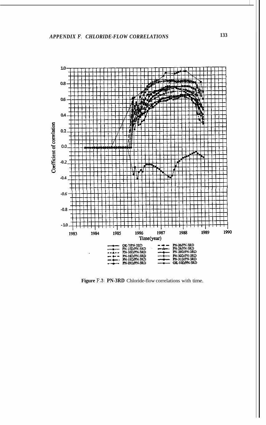
APPENDIX F. CHLORIDE-FLOW CORRELATIONS 133
1.0
0.8
0.6
0.4
0.2
0.0
-0.2
-0.4
-0.6
-0.8
- 1.0
Figure F.3: PN-3RD Chloride-flow correlations with time.
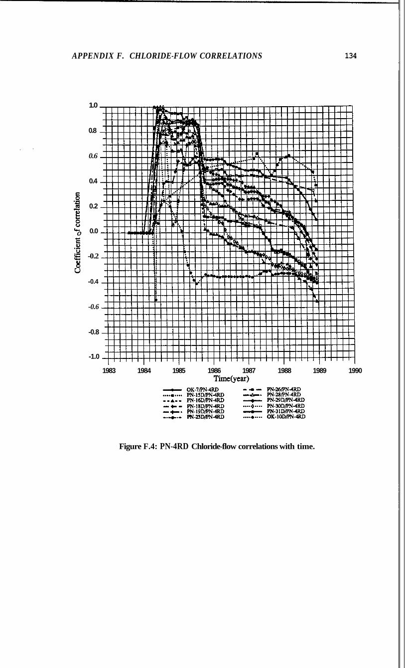
APPENDIX F. CHLORIDE-FLOW CORRELATIONS 134
ru 0
1.0
0.8
0.6
0.4
0.2
0.0
-0.2
-0.4
-0.6
-0.8
-1.0
1983 1984 1985 1986 1987 1988 1989 1990 Timebear)
Figure F.4: PN-4RD Chloride-flow correlations with time.
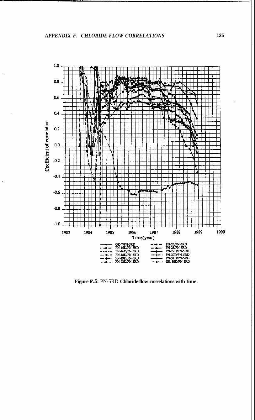
APPENDIX F. CHLORIDE-FLOW CORRELATIONS 135
Figure F.5: PN-5RD Chloride-flow correlations with time.
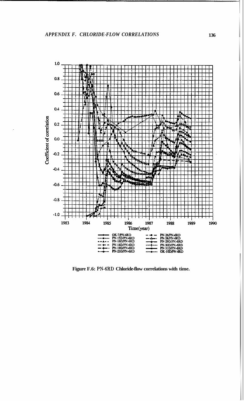
APPENDIX F. CHLORIDE-FLOW CORRELATIONS 136
Figure F.6: PN-6RD Chloride-flow correlations with time.
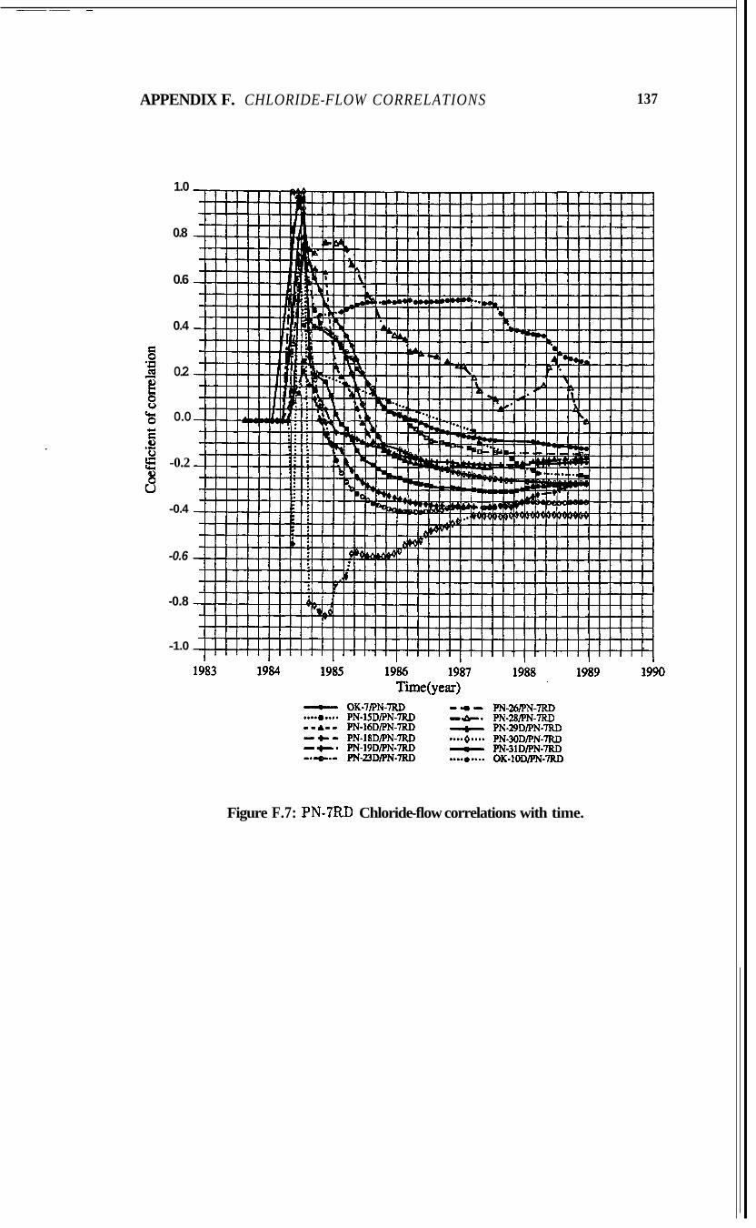
~~~ ~
APPENDIX F. CHLORIDE-FLOW CORRELATIONS
1.0
0.8
0.6
0.4
0.2
0.0
-0.2
-0.4
-0.6
-0.8
-1.0
137
Figure F.7: PN-7RD Chloride-flow correlations with time.
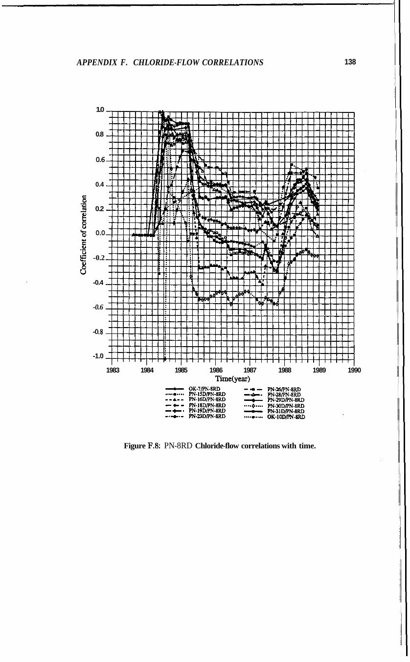
APPENDIX F. CHLORIDE-FLOW CORRELATIONS 138
1.0
0.8
0.6
0.4
0.2
0.0
-0.2
-0.4
-0.6
-0.8
-1.0
1983 1984 1985 1986 1987 1988 1989 1990 Time(year)
Figure F.8: PN-8RD Chloride-flow correlations with time.
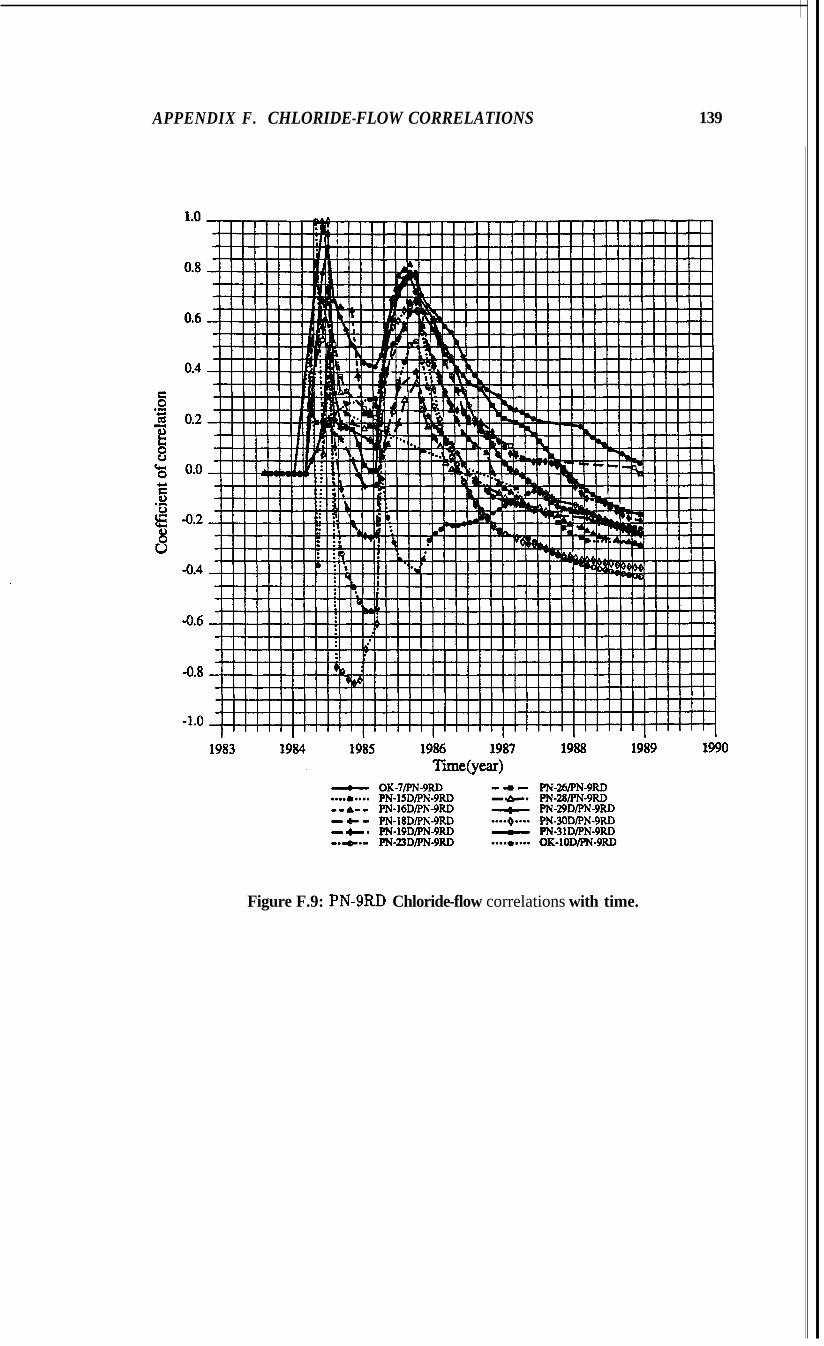
APPENDIX F. CHLORIDE-FLOW CORRELATIONS 139
Figure F.9: PN-9RD Chloride-flow correlations with time.
Appendix G
Chloride Shift-Flow Correlation
140
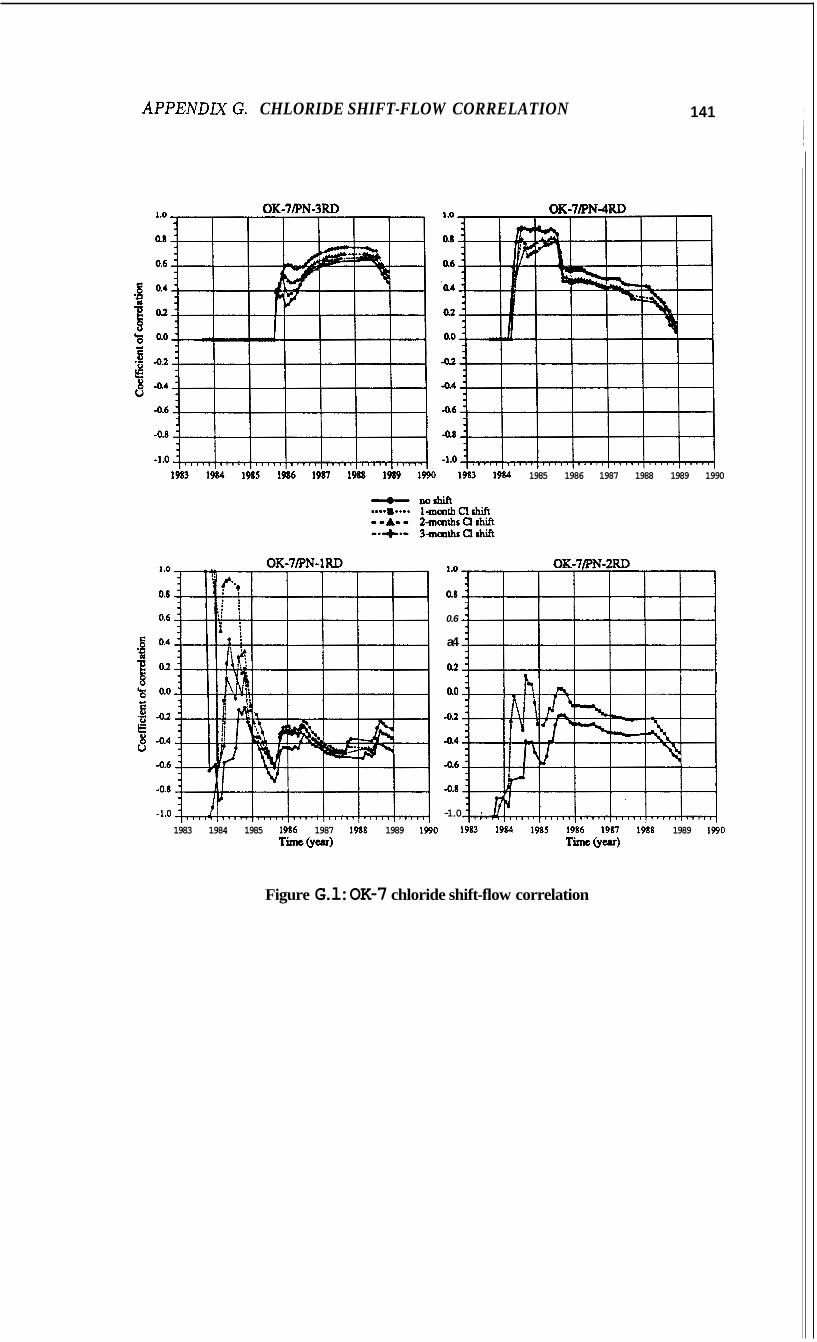
APPEND= G. CHLORIDE SHIFT-FLOW CORRELATION 141
.^ OK-7PN-4RD
1990 1983 1984 1985 1986 1987 1988 1989 1990
1983 1984 1985 ls%6 1987 168 1989 1990 Time(Yur)
._ OK-7PN-2RD
0.6
a4
0.7.
4.2
4.4
-0.6
-0.8
-1.0 1983 19& 1 9 k 1986 19FI 19%8 1989 19bO
T i m (Year)
Figure G.l: OK-7 chloride shift-flow correlation
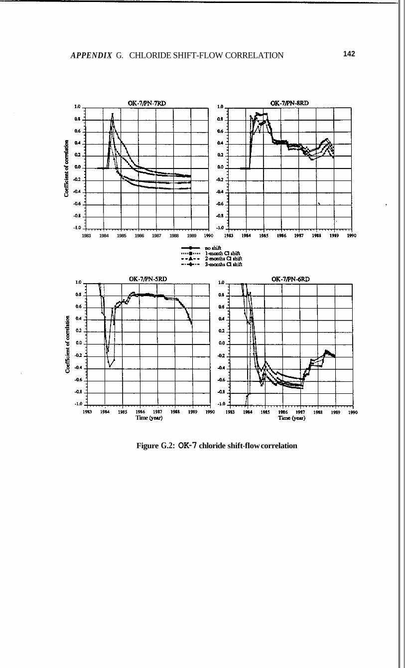
APPENDIX G. CHLORIDE SHIFT-FLOW CORRELATION 142
1983 1984 1985 1986 1987 1988 1989 1990
Time @ear) Time@car)
Figure G.2: OK-7 chloride shift-flow correlation
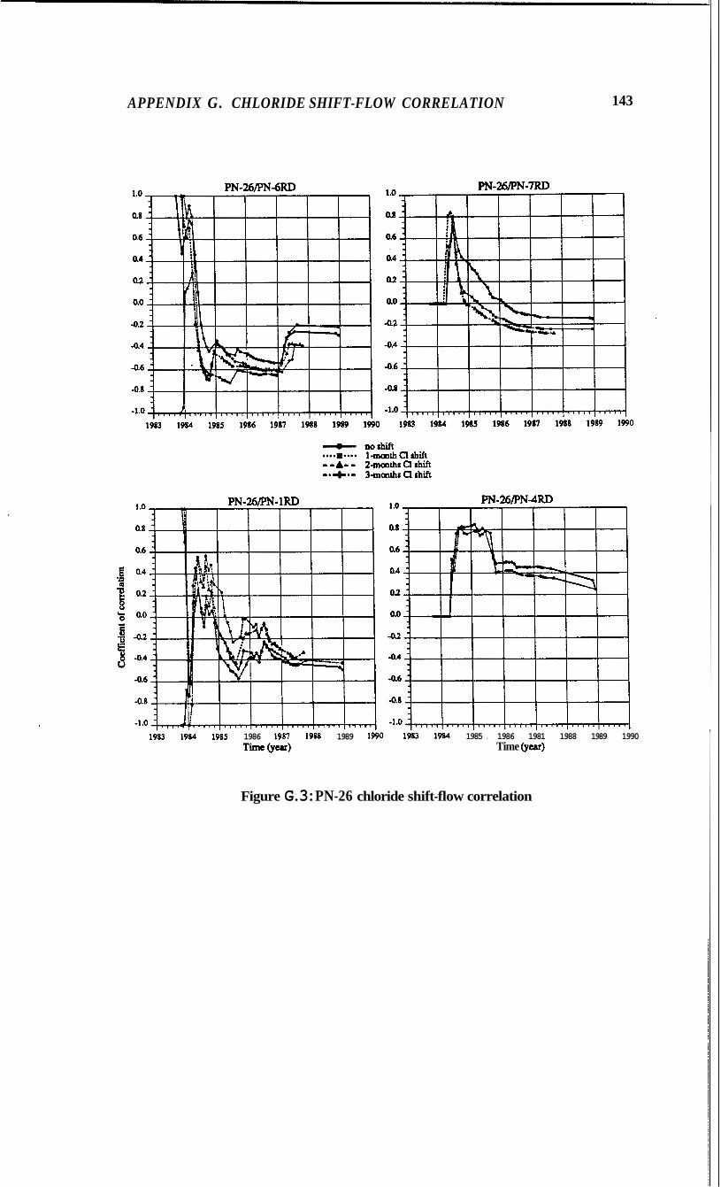
APPENDIX G. CHLORIDE SHIFT-FLOW CORRELATION 143
-.. PN-26PN-lRD
1k 1 9 b lk5 1986 19(n 1998 1989 1990 Time(yesr)
1983 1984 1985 . 1986 1981 1988 1989 1990 Time bear)
Figure G.3: PN-26 chloride shift-flow correlation
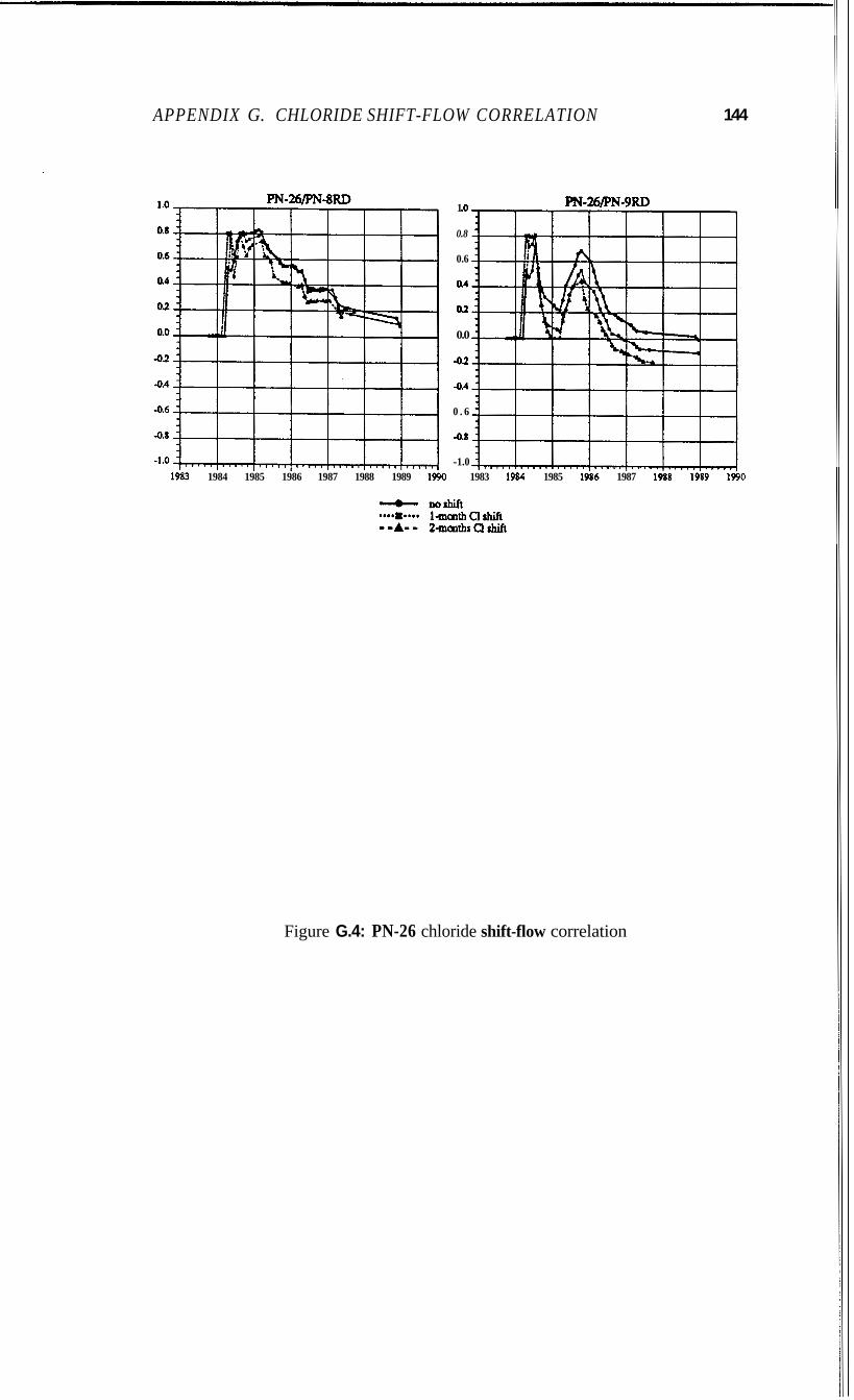
APPENDIX G. CHLORIDE SHIFT-FLOW CORRELATION 144
1 .o PN-26tPN-9R.D
0.8
0.6
OA
0.2
0.0
4.2
-0.4
0 . 6
4.8
-1.0 . . . . . . . . . . . . . . . . . . . . . . . . . 1903 1984 1985 1986 1987 1988 1989 19bO 1983 1984 1985 1986 1987 1 9 b lds9 1 9 b O
Figure G.4: PN-26 chloride shift-flow correlation
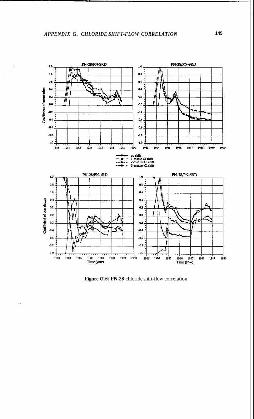
APPENDIX G. CHLORIDE SHIFT-FLOW CORRELATION 145
19k 1984 lds5 1 k 6 1987 1ds8 1989 19bo
... PN-28PN-lRD .^ PN-28PNdRD 1 .U
0.8
0.6
0.4 j 0.2
% 0.0 - .E -0.2 E 8 -0.4 u
-0.6
-0.8
-1.0
1983 1984 1985 1986 1981 1988 1989 1990 Time @car)
1983 1984 1985 1986 1987 1988 1989 1990 Time @car)
Figure G.5: PN-28 chloride shift-flow correlation
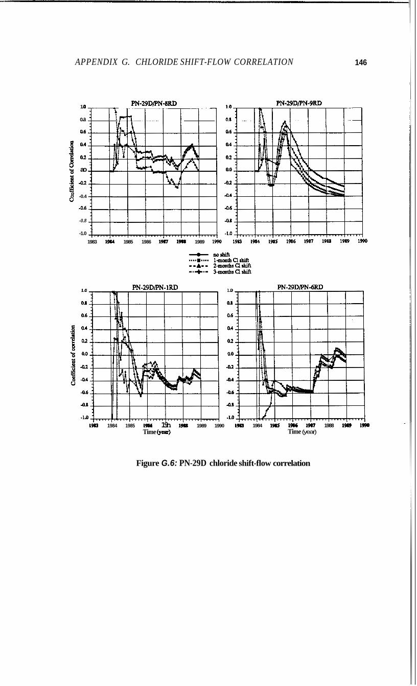
APPENDIX G. CHLORIDE SHIFT-FLOW CORRELATION 146
1 .o
o.a
% ao u
.i -0.2
u 8 -0.4
-0.6
-0.8
-1.0
1983 1984 1985 1986 1981 1988 1989 1990
. A PN-29DPN-1RD .^ PN-29DPN-6RD
1& 1984 1985 1986 19n 19aa 1989 1990 Time (ycrr)
1k 1984 19k 19k 19sr 1988 1& 1990 Time (year)
Figure G.6: PN-29D chloride shift-flow correlation
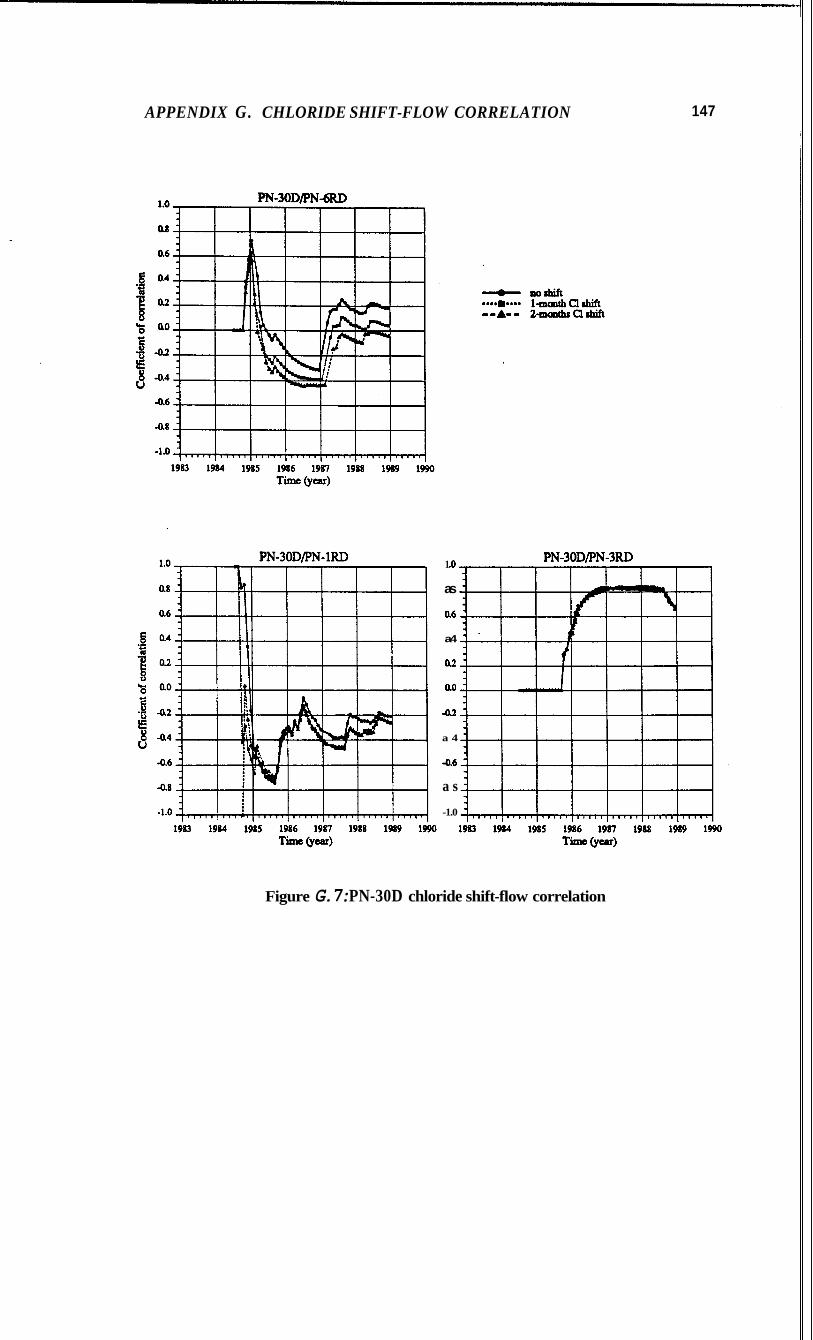
APPENDIX G. CHLORIDE SHIFT-FLOW CORRELATION 147
1 .o
as
a4
0.2
ao
a 4
4.6
a s
-1.0
PN-30DPN-3RD
Figure G.7: PN-30D chloride shift-flow correlation
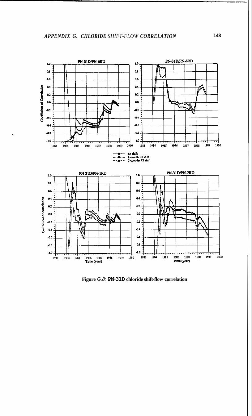
APPENDIX G. CHLORIDE SHIFT-FLOW CORRELATION 148
1983 1984 1985 1986 1987 1988 1989 1990 1683 1984 1985 1986 1987 1988 1989 1990
_ - PNJlDPN-lRD
lk 1984 1 9 k 1986 1987 19eS 1989 1990 Time(year)
1983 1984 19i5 1986 1987 TimeQear)
1988 1989 1990
Figure G.8: PN-31D chloride shift-flow correlation

Appendix H
Chloride-Cumulative Flow Correlation
149
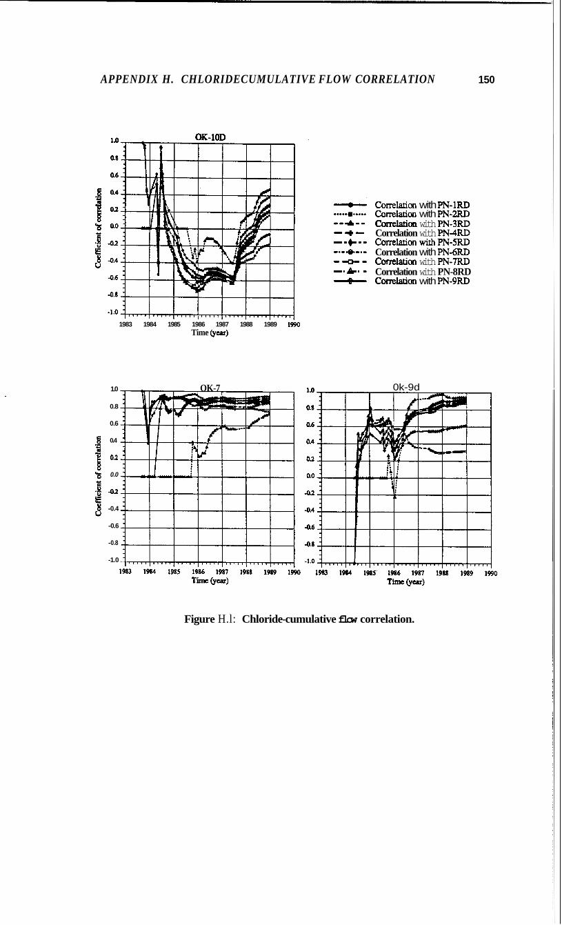
APPENDIX H. CHLORIDECUMULATIVE FLOW CORRELATION 150
1983 1984 1985 1986 1987 1988 1989 1990 Time ear)
correlation with PN-1RD carrelatian with PN-2RD correlat i~~~ with PN3RD
Correlation withPN-SRD
Cofielati~n with PN-7RD Correlation with PN-8RD C~rreati~n with PN-9RD
Correlation with PN4RD
Correlation with PNdRD
1.0 OK-7
0.8
0.6
0.4
0.2
0.0
-0.4
-0.6
-0.8
-1.0
r n 0k-9d
Figure H.l: Chloride-cumulative flow correlation.
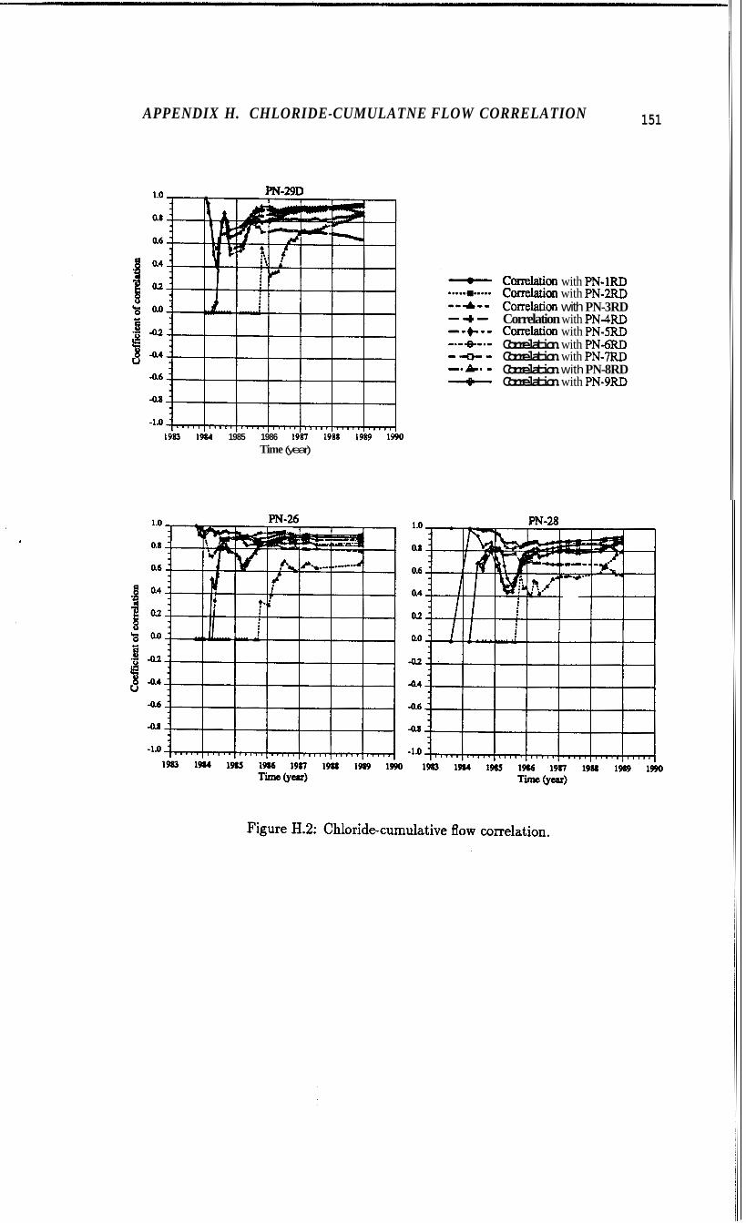
APPENDIX H. CHLORIDE-CUMULATNE FLOW CORRELATION 151
Correlation with PN-1RD Correlation with PN-2RD Conelation with PN-3RD
Correlaei~n with PN-SRD Correlation with PN-4RD
Correlation with PN-6RD Correlation with PN-7RD Correlation with PN-8RD Correlation with PN-9RD
1983 1984 1985 1986 198'1 1988 1989 19bo Time (year)
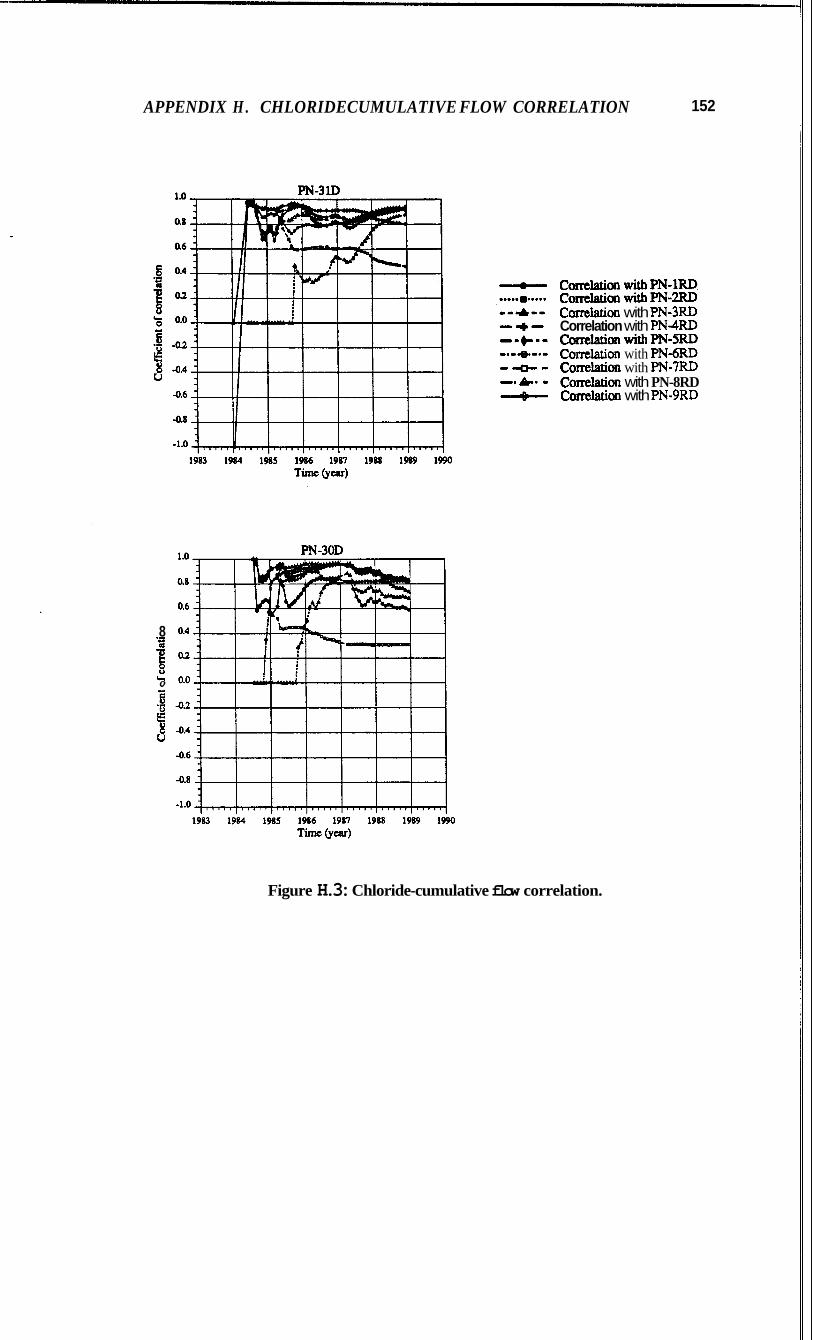
APPENDIX H . CHLORIDECUMULATIVE FLOW CORRELATION 152
cornlation withPN-1RD camlatianwithPN-2RD Cmreiati~n with PN3RD Correlation with PN4RD CorreMcmwithPN-sRD Carrelation with PN-6RD Correlatim with PN-7RD Correlati~n with PN-8RD Correlati~n with PN8RD
B 8
L 0
Figure H.3: Chloride-cumulative flow correlation.

Appendix
Chloride Deviation-Flow Correlation
153
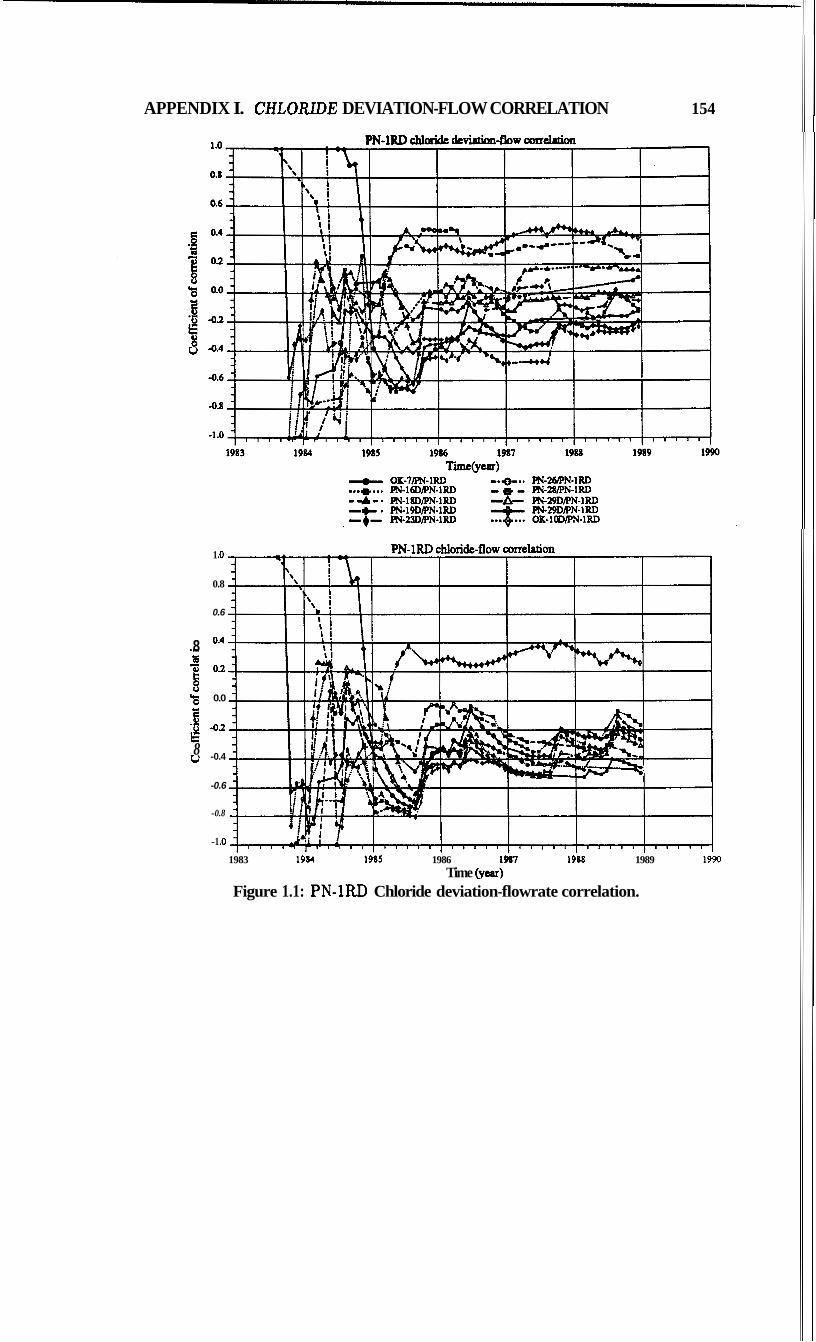
APPENDIX I. CHLOlUDE DEVIATION-FLOW CORRELATION 154
1 .o PN-1RD chlori&flow cornlation
0.8
0.6
.I 8 OA
d O3
Y
"0 0.0
-z 4.2 t: u -0.4 8
3
-0.6
-0.8
-1 .o 1983 1984 1985 1986 19%1 19118 1989 1990
Time bear) Figure 1.1: PN-1RD Chloride deviation-flowrate correlation.
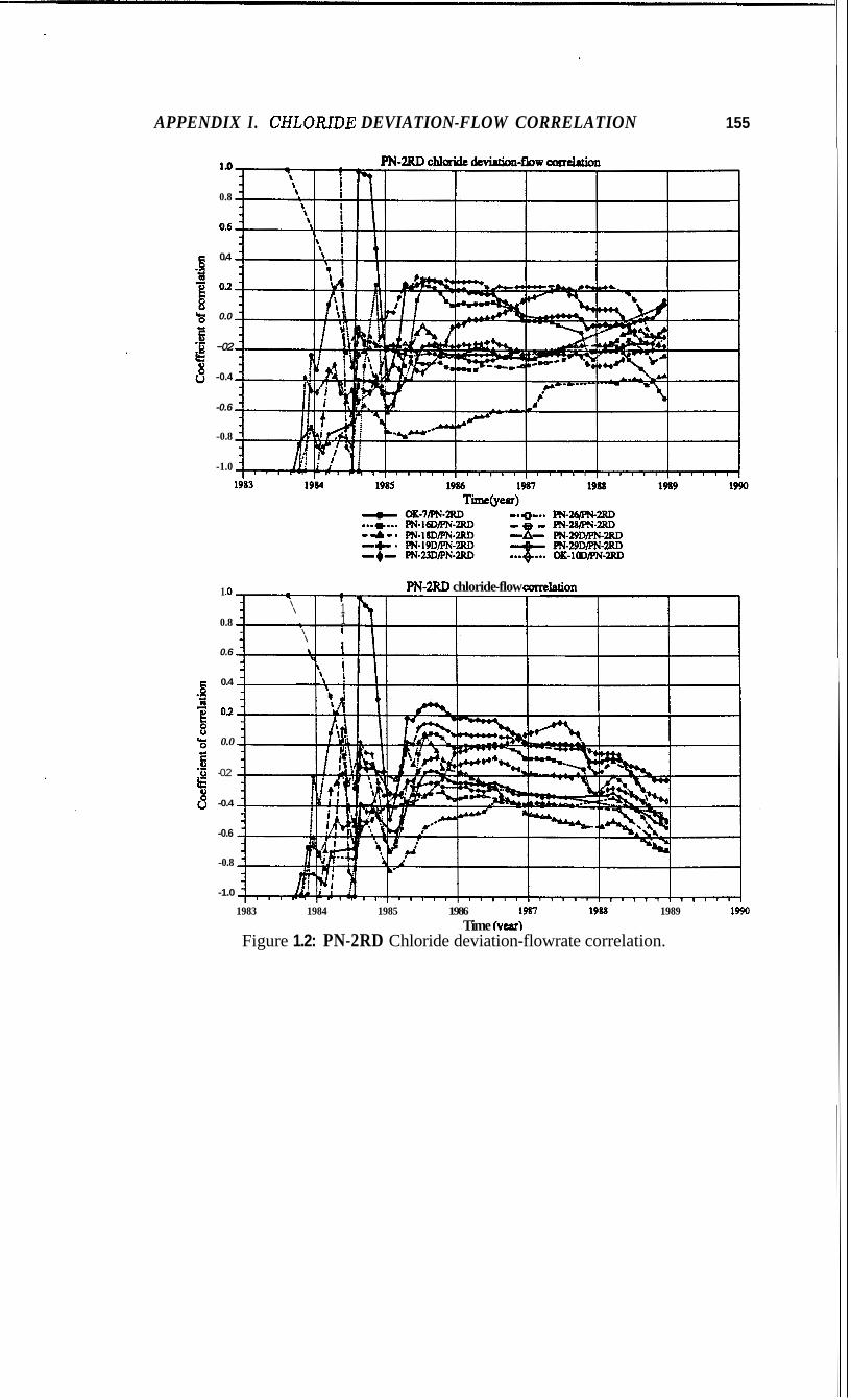
APPENDIX I. CHLORIDE DEVIATION-FLOW CORRELATION 155
1.0
0.8
0.6
0.4
02
0.0
-02
-0.4
-0.6
-0.8
-1.0
1 .o
0.8
0.6
0.4
0.2
0.0
-0.2
-0.4
-0.6
-0.8
-1.0
PN-2RD chloride-flow amdarim -9
\ 1
\ 1 1
\ 1 \ \, i
1 1 h i
1983 1984 1985 1986 1981 1988 1989 1990 Time h e a r )
Figure 1.2: PN-2RD Chloride deviation-flowrate correlation.
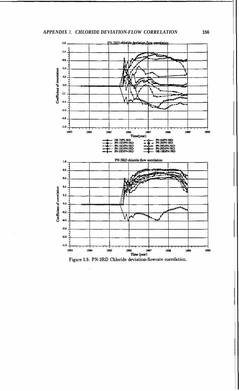
APPENDIX I. CHLORIDE DEVIATION-FLOW CORRELATION 156
1.0 PN-3RD Chlaride deviarion-flow codat ion 1 i i i i i i
0.8
0.6
i i
i 1 i
0.4
0.2
0.0
-0.2
-0.4
-0.6
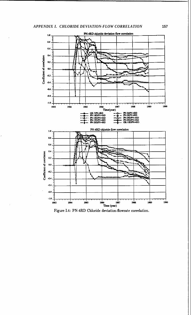
APPENDIX I. CHLORIDE DEVIATION-FLOW CORRELATION 157
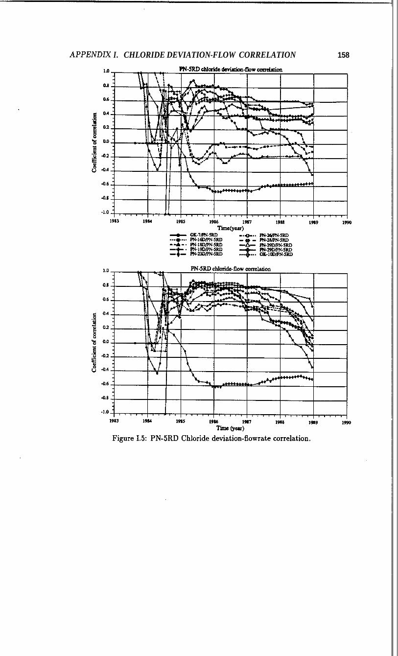
APPENDlX I. CHLORIDE DEVIATION-FLOW CORRELATION 158
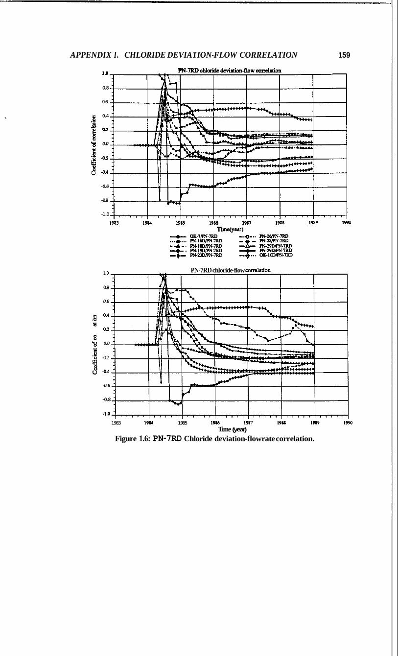
APPENDIX I. CHLORIDE DEVIATION-FLOW CORRELATION 159
1.0
0.8
0.6
g 0.4
a .-
B O3 'E; 0.0
-0.6
-0.8
-1.0
1 .o PN-7RD chloride-flow coxrehion
0.8
0.6
.- 8 0.4 3
0.2
8 'i; 0.0
'E -0.2 k u -0.4 8
0
-0.6
-0.8
- l ~ o I ' ' ' ' ' , ' ' ' ' I , , , , , , , I I I I I
1983 1W 1985 1966 1987 1915 1989 1990 1
Time (year) Figure 1.6: PN-7RD Chloride deviation-flowrate correlation.
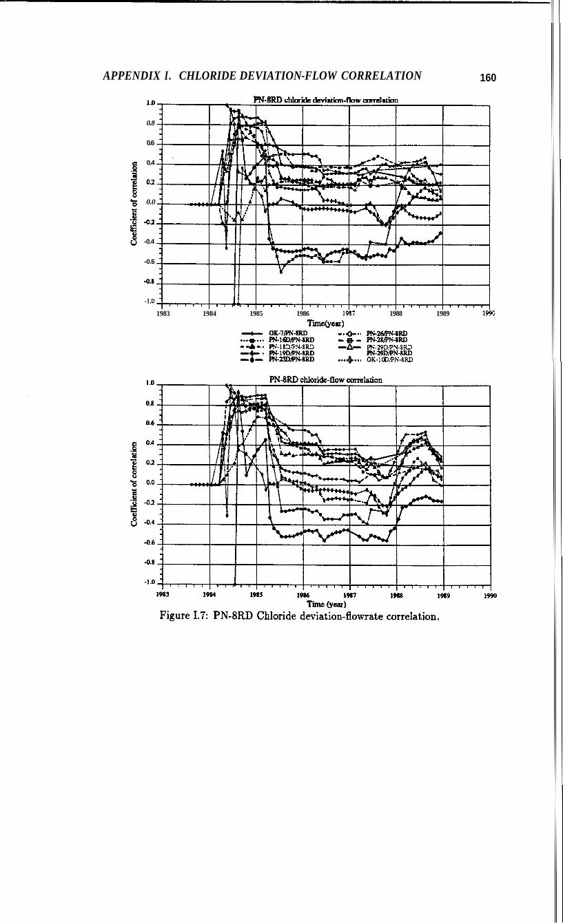
APPENDIX I. CHLORIDE DEVIATION-FLOW CORRELATION 160
1.0
0.8
0.6
g 0.4
-a
% 0.0
z u -0.4 8
-0.6
-0.8
-1 .o 1983 1984 1985 1986 1987 1988 1989 1990
ThQCAiT) + OK-IIIW8RD ...+... PN-16Drn-8RD
-.e-.. PN-26m4RD - 4 - a PN-1 8DPN-8RD - PN-28rn-8RD
-+ * PN-19D/PN-8RD PN-29DPN-8RD OK-IODIPN-IIRD
12- PN-29DPN-8RD
Appendix J
Chloride Deviation-Flow Program Code
161
APPENDIX J . CHLORIDE DEVIATION-FLOW PROGRAM CODE 162
c This program aims to find the correlation coefficient (r) between a c production w.ell’s Chloride residual or deviation from the best fit c line and an injection well’s flow rate with time.
program rescorr implicit real*8 (a-h, 0-2)
dimension tprod(2001, tinj (2001, dev(2001, flow(200) dimension datal(2001, data2(200), data3(200) dimension dummyl(2001, dummy2(200), dummy3(200) character*l5 infilel, infile2, outfile, pltfile character*6 prodwell, injwell write (6,101 ’ Input file name 1 (Preg.plt1 : ’
10 format (a,$) read (5,201 inf ilel
15 format (a61 20 format (a151
write (6,101 ’ Input file name 2 (Rinj .dat) : ’ read (5,201 inf ile2 write (6,101 ’ Output file name (P-Rdev.cor) : ’ read (5,201 outf ile write (6,101 ’ Plot file name (P-Rdev.plt) :
read (5,201 pltfile write (6,101 ’ Production well . ’ read (5,151 prodwell write (6,101 ’ Injection well . , read (5,151 injwell write (6,101 ’ Lag time in months . ’ read (5,251 nt
25 format (i2) open (unit-1 ,status=’old’ ,f ile=inf ilel) open (unit=2,status=’old’ ,filerinfile21 open (unit=3, status=’unknoun’ ,file=outf ile) open (unit=4,status=’~nknom’ ,file=pltf ile) nprod = 1
APPENDIX J. CHLORIDE DEVIATION-FLOW PROGRAM CODE 163
30
100
40
200
210
220
350
read (1, * , end=lOO) tprod(nprod1, dev (nprod) nprod = nprod + 1
goto 30 nprod = nprod - 1
n i n j = 1
read (2,*,end=200) t i n j ( n i n j 1 , flow(ninj1 n i n j = n i n j + 1
goto 40
n i n j = n i n j - 1
k = l i - 1
i f ( i .gt . nprod ) goto 350 j = l
if ( tprod( i ) .eq. t i n j ( j > ) then
dummyl(k1 = tp rod( i ) dummy2(k) = dev(i) dummy3(k) = f low(j) k = k + l i = i+1
goto 210
else
j = j + i
i f ( j .gt. n in j ) then i = i + 1
goto 210 endif
goto 220 endif ndata = k-1
n n = n t + l i = l
do 400 k= nn, ndata
if ( dummy2(k-nt) . ge . 1 .El0 ) Roto 400
APPENDIX J. CHLORIDE DEVIATION-FLOW PROGRAM CODE 164
400
40 1
402
403
404
405
406
407
410
412
415
420
datal(i) = dummyl(k)
data2(i) = dummyZ(k-nt) data3(i) = dummy3(k) i = i + 1
continue
ndata = i - 1 write (3,401) format (’ ’1 write (3,402)
format (’ ’1 write (3,403)
format 0 ’1 write (3,404) prodwell, injwel1,nt format (’ ’,lOx,a6, ’/’,a6, ’ Cldev-Flow CORRELATION with LAG of’,
8 i2, ’ MONTH(S)’) write (3,405) format ( J ’,lox, ~,,,,,---,,,---------------------------------’,
& ’--------------’ write (3,406)
format (’ ’1 write (3,407) ’TIME’, ’R’ , ’R**2’, ’SIC’, ’Sy’
format ( ’ ,5x, a4, lox, a,9x, a4, Ilx, a2,14x, a2) mdata = ndata-1 write (4,410) mdata
format (i3)
do 420 i = 2 ,ndata call coeff (i,data2,data3,r,r2,sx,sy) m i t e (3,412) datal(i1, r, r2, sx, sy format (2x,fl0.4,2x,f10.6,2x,flO.6,2f15.5)
write (4,415) datal(i), r format (fl0.4,lx,f10.6)
continue
close (unit=l)
1

APPENDIX J. CHLORIDE DEVIATION-FLOW PROGRAM CODE 165
close (unit-2) close (unit-3) end
C
C
subroutine coeff ( n, data2 , data3 , r, r2 , sx , sy )
implicit real*8 (a-h, 0-2)
dimension data2(200) , data3(200) devsum = 0. flowsum = 0.
sqdevsum = 0. sqflowsum = 0. sumdevflow = 0. do 10 i = 1,n
devsum = devsum + data2(i) flowsum = flowsum + data3(i) sqdevsum = sqdevsum + data2(i)*data2(i) sqflowsum = sqflowsum + data3(i)*data3(i) sumdevflow = sumdevflow + data2(i)*data3(i)
10 continue
if (flowsum .eq. 0 . 0 ) goto 99
xn = real(n) xbar = devsum/xn ybar = flowsum/xn syl = (sqflowsum - flowsum*flowsum/xn)/xn sy = sqrt(sy1) if (sy .eq. 0 . 0 ) return
8x1 = (sqdevsum - devsum*devsum/xn)/xn sx = sqrt(sx1) r = (sumdevf low - xn*xbar*ybar)/(xn*sx*sy) 1-2 = r*r
99 return
end
Appendix K
Linear Combination Program Code and Output
166
APPENDIX K. LINEAR COMBINATION PROGRAM CODE AND OUTPUT167
program lincomb4 c-------------------------------------------------------------------
c This program computes for the solution of the linear combination c method where chloride is expressed as a linear combination of c the injection flowrates. The input file tabulates the chloride c trend with time of a production well and the flowrates of the c injection wells corresponding t o the chloride measurements. c-------------------------------------------------------------------
implicit real*8 (a-h, 0-2)
dimension a(10,lO) ,rhs(lO) character*l5 filename character*8 pname,riname(9) dimension flow(9) ,need(9) ,dumflow(9)
C
do i = 1,lO rhs(i) = 0. do j = 1,lO a(i,j) = 0.
enddo enddo write (6,101 ’File Name For Calculation (*bal.out) : ’
10 format (a40,$) read (5,201 filename
20 format (a15) open (unit=l ,status=’old’ ,f ile=f ilename) open (~nit=2,status=’unknown’ ,file=’soln.dat’) read (1,301 pname,nri,(riname(i), i=1,9)
30 format (a8,lx,i2,9(lx,a8)) write (6,401 ’Available Reinjection Wells a r e : ’
40 format (10x,a35) do i = 1,nri
write (6,501 i, riname(i) 50 format (i2,5x,a8)
APPENDIX K. LINEAR COMBINATION PROGRAM CODE AND OUTPUT168
enddo
55 write (6,601 ’Number of wells t o be included i n computation’
60 format (a461
write (6,701 ’ (min = 1, max = 9) : ’ 70 format (a21, $1
read (5,801 nwells 80 format ( i3)
i f ( w e l l s .It. 1 .or . nwells .gt. 9) goto 55
i f (nvells .eq. 9) then
do i = 1,9
need(i) = i
enddo
goto 105
90
100
105
110
120
130
140
150
endif
write (6,901 ’Type the number corresponding t o the wells needed’
format ( a50 )
do i = 1,nwells
read(5,lOO) need(i) format (i2)
enddo
write (6,110) ’Time interval needed i n computation : ’ format (a38)
write (6,120) ’Tmin : ’ format (a”,$)
read (5,130) tmin
format (f 10.4)
write (6,120) ’Tmax : ’ read (5,130) tmax
write (2,140) ’Production Well : ,pname
format (a40, a8)
write (2,150) ’Number of Reinjection Wells Included : ’ ,nuells format (a40, i2)
do i = 1,nwells
APPENDIX K . LINEAR COMBINATION PROGRAM CODE AND OUTPUT169
160
170
180
200
210
write (2,160) i,riname(need(i))
format (10x,il,5x,a8)
enddo
write (2,170) 'Time Interval Considered
format ( a40 1 write (2,180) 'Tmin = ' ,train write (2,180) 'Tmax = ' ,tmax format (10x,a7,f10.4)
kp = 1
read (1,21O,end=1000) time,cl,(flow(i), i=l,nri)
if (kp.eq.1) c10 = cl format (f'10.4,2x,f6.0,9f8.2)
if ( time .It. tmin .or. time .gt. tmax 1 goto 200 do i = 1,nwells
. '
if (flou(need(i)) .eq. -99.) goto 200 dumflow(i) = flow(need(i))
enddo
nromax = nwells + 1 do i = 2,nromax
a(1,i) = a(1,i) + dumflou(i-1) a(i,l) = a(i,l) + dumflow(i-1)
do j = 2,nromax a(j ,i> = a(j ,i) + dumflow(i-l)*dumflou(j-l)
enddo
enddo
rhs(1) = rhs(1) + cl do i = 2,nromax
rhs(i) = rhs(i) + dumflow(i-l)*cl enddo
k p = k p + l goto 200
1000 p = kp - 1 C a(1,i) = p
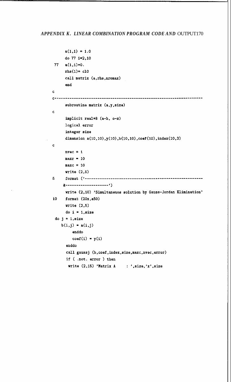
APPENDIX K . LINEAR COMBINATION PROGRAM CODE AND OUTPUT170
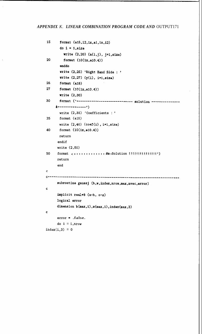
APPENDIX K. LINEAR COMBINATION PROGRAM CODE AND OUTPUT171
write (2,351 ’Coefficients : ’ 35 format (a151
write (2,401 (coef (i) , i=l,size) 40 format (lO(lx,elO.4))
return endif write (2,50)
50 format (I!!!!!!!!!!!!!!! No Solution !!!!!!!!!!!!!!!’) return
end C
error = . fa lse .
do i = 1,nrow indax(i,3) = 0
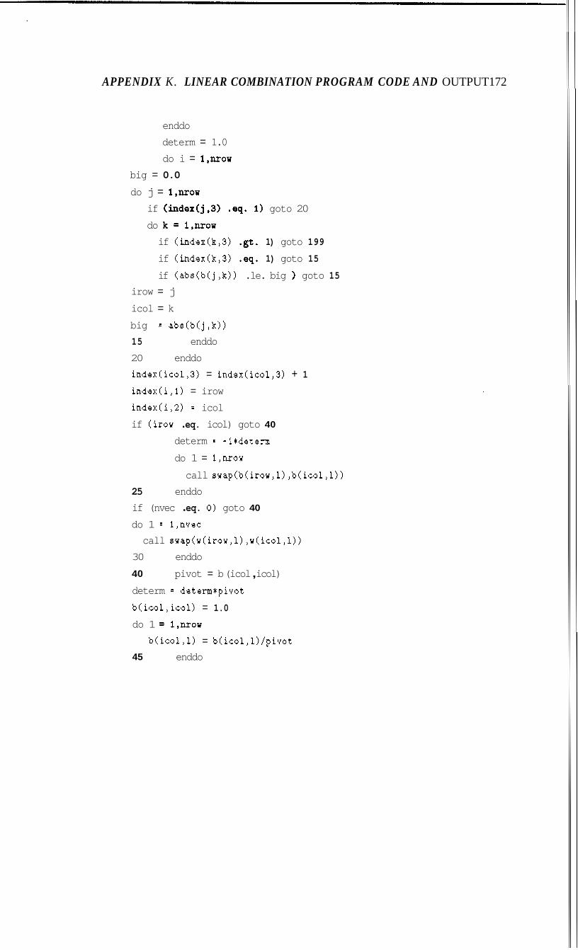
APPENDIX K. LINEAR COMBINATION PROGRAM CODE AND OUTPUT172
enddo determ = 1.0 do i = 1,nrow
big = 0.0
do j = 1,nrow if (index(j,3) .eq. 1) goto 20 do k = 1,nrow if (index(k,3) .gt. 1) goto 199 if (index(k,3) .eq. 1) goto 15 if (abs(b(j,k)) .le. big goto 15
irow = j icol = k big = abs(b(j,k)) 15 enddo 20 enddo index(icol,3) = index(icol,3) + 1 index(i,l) = irow index(i,2) = icol if (irou . eq. icol) goto 40
determ = -l*determ do 1 = 1,nrow call suap(b(irow,l) ,b(icol,l))
25 enddo if (nvec . eq. 0) goto 40
do 1 = 1,nvec call swap(w(irou,l) ,w(icol,l))
30 enddo 40 pivot = b (icol , icol) determ = determ*pivot b(ico1,icol) = 1.0 do 1 = 1,xuow
b(ico1,l) = b(icol,l)/pivot 45 enddo
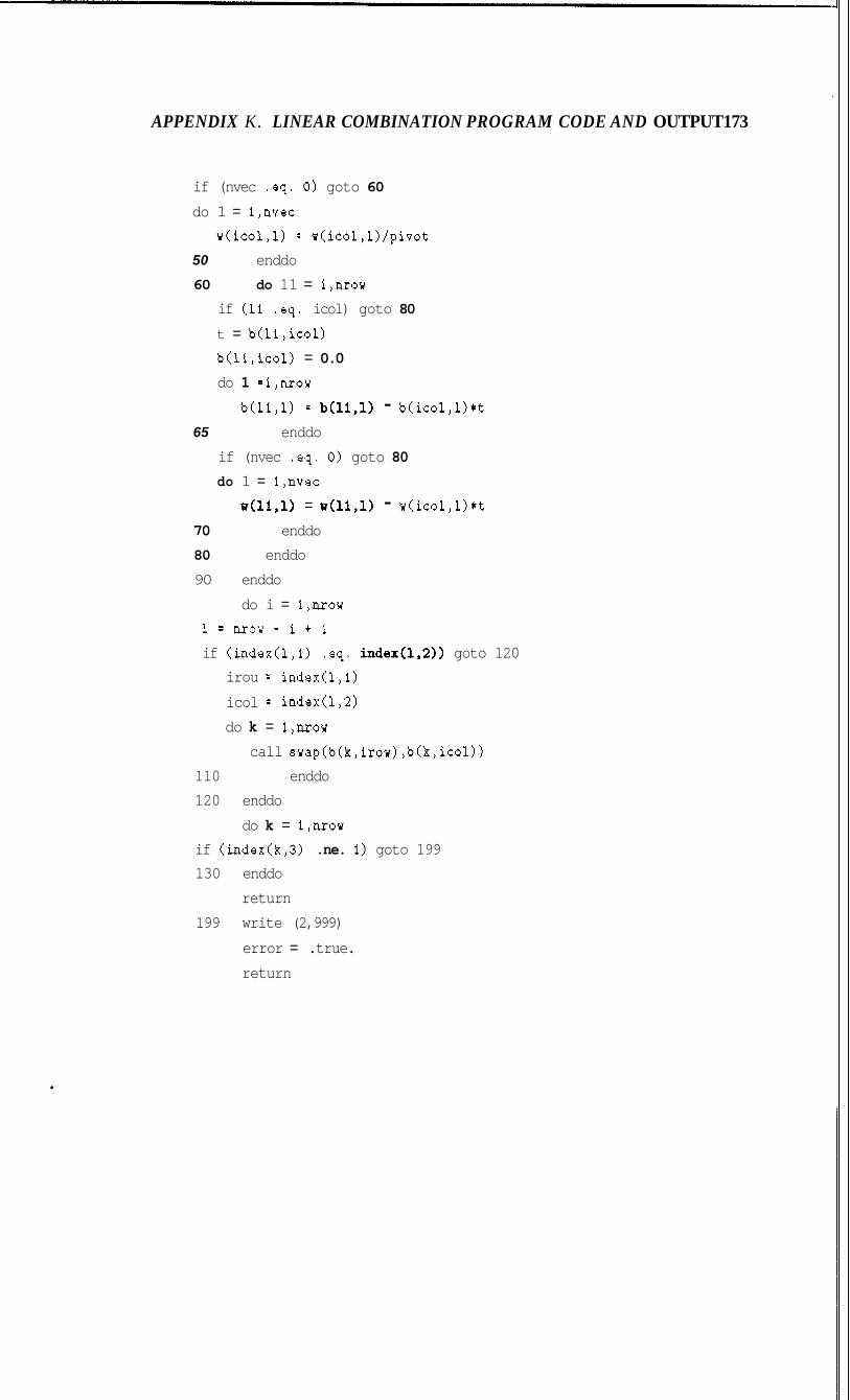
APPENDIX K. LINEAR COMBINATION PROGRAM CODE AND OUTPUT173
if (nvec .eq. 0) goto 60 do 1 = 1,nvec
u(ico1,l) = u(icol,l)/pivot 50 enddo 60 do 11 = 1,nrou
if (11 .eq. icol) goto 80 t = b(l1 ,icol) b(l1,icol) = 0.0 do 1 =l,nrou
b(l1,l) = b(ll,l) - b(icol,l)*t 65 enddo
if (nvec .eq. 0) goto 80 do 1 = 1,nvec
u(li,l) = u(l1,l) - u(icol,l)*t 70 enddo 80 enddo 90 enddo
do i = 1,nrow l = n r o u - i + l if (index(1,l) .eq. index(l,2)) goto 120
irou = index(1,l) icol = index(l,2) do k = 1,nrou
call suap(b(k,irow) ,b(k,icol)) 110 enddo 120 enddo
do k = 1,nrou if (index(k,3) .ne. 1) goto 199 130 enddo
return 199 write (2,999)
error = .true. return
APPENDIX K. LINEAR COMBINATION PROGRAM CODE AND OUTPUT174
999 format ( ’ error -- matrix singular ’> end
C
implicit C
hold = a
a = b
b = hold
return end
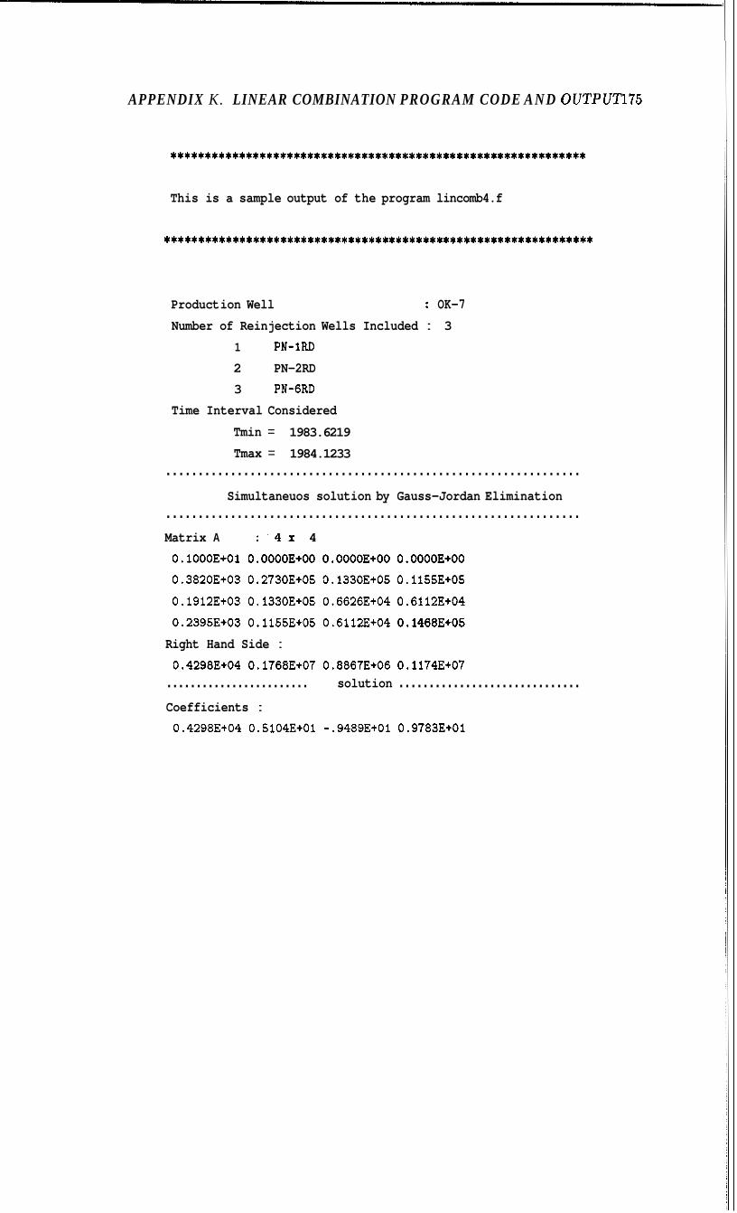
APPENDIX K. LINEAR COMBINATION PROGRAM CODE AND OUTPUT175
. . . . . . . . . . . . . . . . . . . . . . . . . . . . . . . . . . . . . . . . . . . . . . . . . . . . . . . . . . . . .
This is a sample output of the program lincomb4.f
. . . . . . . . . . . . . . . . . . . . . . . . . . . . . . . . . . . . . . . . . . . . . . . . . . . . . . . . . . . . . . .
Product ion Well : OK-7 Number of Reinjection Wells Included : 3
1 PN-1RD 2 PN-2RD 3 PN-6RD
Time Interval Considered
Tmin = 1983.6219
Tmax = 1984.1233 ................................................................
Simultaneuos solution by Gauss-Jordan Elimination ................................................................ Matrix A : . 4 x 4
O.l000E+01 0.0000E+OO 0.0000E+OO 0.0000E+OO
0.3820E+03 0.2730E+05 0.1330E+05 0.11553+05
0.1912E+03 0.1330E+05 0.66263+04 0.6112Et04
0.23953+03 0.11553+05 0.6112E+04 0.1468E+05
Right Hand Side : 0.42983+04 0.1768E+07 0.8867E+06 0.11743+07
........................ solution .............................. Coefficients : 0.42983+04 0.5104E+Ol -.9489E+Ol 0.97833+01

Bibliography
[l] Amistoso, A. E., Aquino, B. G., Aunzo, 2. P., Jordan, 0. T., Sta.Ana, F. X., Bodvarsson, G., and Doughty, C.: “Reservoir Analysis and Numeri-
cal Modelling of the Palinpinon Geothermal Field, Negros Oriental, Philip- pines,” PNOC-Energy Development Corporation and Lawrence Berkeley Laboratory, Fort Bonifacio, Makati, Metro Manila, PHILIPPINES (March
1990) UN-DTCD Project PHI/86/006.
[2] Harper, R. T. and Jordan, 0. T.: “Geochemical Changes in Response to
Production and Reinjection Palinpinon-I Geothermal Field, Negros Oriental,
Philippines,” Internal Memo (1985).
[3] IMSL, Inc.: “ZXOLP,” The IMSL Library, Houston, TX (1982) 4,
zxoLP-1-zxoLP-17.
[4] Los Alamos National Laboratory, NM: “Geothermal Program Review,” No.
Report No. CONF-8704110-, Los Alamos National Laboratory and Merid-
ian, Corp., New Mexico (April 1987).
[5] Lovekin, J.: “Optimization of Injection Scheduling in Geothermal Fields,”
No. SGP-TR-112, Stanford Geothermal Program, Stanford University (May
1987).
[6] Luenberger, D. G.: Linear and Nonlinear Programming, 2 edition, Addison-
Wesley, Reading, Massachusetts (1984).
[7] Urbino, M. E., Malate, R. M., Bueza, E. L., Zaide, M. C., Garcia, S. E., Hermoso, D. Z., and Jordan, 0. T.: “PN-9RD Tracer Test: An Integrated
176

BBLIOGRAPHY 177
Report,” PNOC-Energy Development Corporation, Fort Bonifacio, Makati, Metro Manila, PHILIPPINES (May 1986) Internal Report.