This article was downloaded by: [University of Lethbridge]On: 03 October 2014, At: 01:09Publisher: Taylor & FrancisInforma Ltd Registered in England and Wales Registered Number: 1072954 Registered office: Mortimer House,37-41 Mortimer Street, London W1T 3JH, UK

IIE TransactionsPublication details, including instructions for authors and subscription information:http://www.tandfonline.com/loi/uiie20

Optimization of discrete event systems viasimultaneous perturbation stochastic approximationMICHAEL C FU a & STACY D. HILL ba College of Business and Management, Institute for Systems Research, University ofMaryland , College Park, MD, 20742, USAb The Johns Hopkins University, Applied Physics Laboratory , Laurel, MD, 20723, USAPublished online: 31 May 2007.

To cite this article: MICHAEL C FU & STACY D. HILL (1997) Optimization of discrete event systems via simultaneousperturbation stochastic approximation, IIE Transactions, 29:3, 233-243, DOI: 10.1080/07408179708966330

To link to this article: http://dx.doi.org/10.1080/07408179708966330

PLEASE SCROLL DOWN FOR ARTICLE

Taylor & Francis makes every effort to ensure the accuracy of all the information (the “Content”) containedin the publications on our platform. However, Taylor & Francis, our agents, and our licensors make norepresentations or warranties whatsoever as to the accuracy, completeness, or suitability for any purpose of theContent. Any opinions and views expressed in this publication are the opinions and views of the authors, andare not the views of or endorsed by Taylor & Francis. The accuracy of the Content should not be relied upon andshould be independently verified with primary sources of information. Taylor and Francis shall not be liable forany losses, actions, claims, proceedings, demands, costs, expenses, damages, and other liabilities whatsoeveror howsoever caused arising directly or indirectly in connection with, in relation to or arising out of the use ofthe Content.

This article may be used for research, teaching, and private study purposes. Any substantial or systematicreproduction, redistribution, reselling, loan, sub-licensing, systematic supply, or distribution in anyform to anyone is expressly forbidden. Terms & Conditions of access and use can be found at http://www.tandfonline.com/page/terms-and-conditions

lIE Transactions (1997) 29, 233-243

Optimization of discrete event systems via simultaneousperturbation stochastic approximation

MICHAEL C. FU1 and STACY D. HILL2

1College of Business and Management, Institute for Systems Research, University of Maryland, College Park, MD 20742. USA2The Johns Hopkins University, Applied Physics Laboratory, Laurel, MD 20723, USA

Received August 1995 and accepted September 1996

We investigate the use of simultaneous perturbation stochastic approximation for the optimization of discrete-event systems viasimulation. Application of stochastic approximation to simulation optimization is basically a gradient-based method, so muchrecent research has focused on obtaining direct gradients. However, such procedures are still not as universally applicable as finite­difference methods. On the other hand, traditional finite-difference-based stochastic approximation schemes require a large numberof simulation replications when the number of parameters of interest is large, whereas the simultaneous perturbation method is afinite-difference-like method that requires only two simulations per gradient estimate, regardless of the number of parameters ofinterest. This can result in substantial computational savings for large-dimensional systems. We report simulation experimentsconducted on a variety of discrete-event systems: a single-server queue, a queueing network, and a bus transit network. For thesingle-server queue, we also compare our work with algorithms based on finite differences and perturbation analysis.

where C is an analytically available function, usuallyrepresenting some cost on the parameter. The problem isto find

8* ~ argmin{J(8) : (} E 8}.

For example, in one problem that we consider - theminimization of mean system time in a queueing network- the jth component of (} is the mean service time at theith station. The stochastic approximation (SA) algorithmfor solving \1J = 0, where '\1' indicates the gradient op-

Like finite-difference-based stochastic approximationprocedures, SPSA uses only estimates of the objectivefunction itself, so it does not require detailed knowledgeof system dynamics and input distributions; hence, it isapplicable to any system that can be simulated. More­over, SPSA requires only two sample estimates to cal­culate a gradient estimate, regardJess of the dimension ofthe parameter vector, and therefore requires significantlyfewer simulations than finite differences for estimatinggradients in high dimensions.

To be more specific, let 8 = ((8)1" .. 1 (8)p) E e c flAP

denote a p-dimensional vector of controllable (adjustable)parameters and OJ the stochastic effects (e.g., the randomnumbers in a simulation), where 8 is a compact set. LetL(8, OJ) denote the sample path performance measure ofinterest, with expectation E[L(8, w)], and define the ob­jective function

1. Introduction

We consider the problem of optimizing a stochastic dis­crete event system under the overriding assumption thatthe system cannot be adequately modeled using analyticalmeans, e.g., optimizing the operations of a complexmanufacturing system. For such systems, simulation isoften used to estimate performance. Under suitable con­ditions, the resulting optimization problem reduces tofinding the zero of the objective function gradient, so thatgradient-based techniques based on stochastic approxi­mation can be applied. Such optimization techniques at­tempt to mimic steepest-descent algorithms from thedeterministic domain of non-linear programming, withtwo major complications: only noisy estimates of systemperformance are available, and gradients are not auto­matically available. Techniques such as perturbationanalysis (PA) or the likelihood ratio method (cf. [1])provide efficient means for estimating gradients based onsimulation sample paths, but these techniques are notuniversally applicable, in which case gradient estimatesbased on finite differences of system performance esti­mates are employed. However, the computational re­quirements of finite-difference methods grow linearly withthe dimension of the controllable parameter vector,making it burdensome for high-dimensional problems.

This paper considers a technique called simultaneousperturbation stochastic approximation (SPSA) that re­quires minimal assumptions on the system of interest [2].

0740·817X © 1997 "lIE"

J(8) = E[L(8, OJ)] + C(8), (1)

Dow

nloa

ded

by [

Uni

vers

ity o

f L

ethb

ridg

e] a

t 01:

09 0

3 O

ctob

er 2

014

234

erator, is given by the following iterative scheme that isbasically the stochastic version of a steepest descent al­gorithm:

8n+1 = ne(8n - Qngn), (2)

where 8n = ((8 n )I" .. , ((}n)p) represents the nth iterate, gnrepresents an estimate of the gradient "VJ at 8n , {an} is apositive sequence of numbers converging to 0, and nedenotes a projection on e. .

Aside from the earlier finite-difference-based work ofAzadivar and Talavage [3], the application of SA to theoptimization of stochastic discrete-event systems has beena fairly recent development, and has been coupled closelywith the emergence of an en tire research area devoted tosimulation-based direct gradient estimation techniques(see [I]). It is well known that these direct gradient esti­mates yield the best convergence rate (cf. [4] and refer­ences therein), and this is borne out in simulationexperiments as well. For example, following the earlierempirical work of Suri and Zazanis [5] and Suri andLeung [6], L'Ecuyer et al. [7] compared a large number ofdifferent SA algorithms on a single-server queue problem(with a scalar parameter), and found that the methodutilizing an infinitesimal perturbation analysis gradientestimator (cf. [8]) outperformed all the others. Otherrelated work includes Fu [9], Andradottir [10], andWardi [11]. However, for many problems direct gradientestimates may not be readily available, in which casegradient estimates based on (noisy) measurements of theperformance measure itself are the only recourse. Whenthe dimension, p, of the parameter is large, traditionalfinite-difference methods can become prohibitively ex­pensive, whereas the method of simultaneous perturba­tions allows the gradient to be estimated with twosimulations using only estimates of the performancemeasure itself. In sum, the SPSA method exhibits threedesi ra bIe characteristics:

(l) generality - its advantage over direct estimationmethods such as PA and the likelihood ratio method is itsapplicability to any system that can be simulated;

(2) efficiency - its advantage over usual finite-differencemethods is its practicality for high-dimensional problems;

(3) ease of use - it is as easy to apply as finite-differencemethods.

SPSA has been applied successfully to nonlinear controlproblems using neural networks [12]. In this paper, weinvestigate the application of SPSA to simulation opti­mization of stochastic discrete-event systems by con­ducting simulation experiments on three differentoptimization problems: a single-server queueing problem,a queueing network problem, and a transportationproblem. Preliminary experimental results were reportedin Hill and Fu [13,14]. In the first example we compare theperformance of SPSA with SA algorithms based on fi­nite-difference estimates and on infinitesimal perturbation

Fu and Hill

analysis estimates. The purpose is not to make definitiveconclusions as to superiority, but simply to demonstratereasonably comparable performance on the smallestmulti-dimensional problem possible (two dimensions).The second example was chosen to test SPSA on a higher­dimensional problem, and the third example attempted totest it on a more 'practical' problem, that of reducingtransfer waiting times in a transit network. Difficultiesexperienced in naive application of the method are dis­cussed. The rest of the paper is organized as follows, InSection 2 we present the simultaneous perturbation gra­dient estimator, contrasting it with the usual finite differ­ence estimator. In Section 3 we describe the three problemsettings. Discussion of convergence for the SPSA algo­rithm applied to the examples is provided in Section 4,with a proof outlined for the single-server queue. The re­sults of simulation experiments are provided in Section 5.Section 6 contains a summary and conclusions.

2. Simultaneous perturbations

In this section, we present and contrast finite differenceestimators and simultaneous perturbation estimators fora performance measure gradient "VE[L]. Let e, denote theunit vector in the ith direction of f!IlP, tn the simulationlength of the nth iteration, Sn the starting state for the nthiteration, Lt(fJ, w,s) the observed (sample) system per­formance at (} on sample path co for duration t startingfrom state s, (?in); the zth component of ?in (an estimate of"VE[L] at ()n), and {cn } a positive sequence converging to O.

The usual symmetric difference (SO) estimator for"VE[L] is given by

(3)

where w~+ and w~- denote the pair of sample paths usedfor the ith component of the nth iterate of the algorithmwith respective starting states s~+ and s~-. If the method ofcommon random numbers is employed, thenro~- = ro~+ = co; (cf. [7]).

Let {An} be an i.i.d. vector sequence of perturbationsof i.i.d. components {(An);, i = 1

2, .. ,p} symmetrically

distributed about 0 with EI(An ) ; I uniformly bounded(see [2] for a definition). Then the simultaneous pertur­bation (SP) estimator is given by

(9n); = (L; - L;)/[2cn(An);], (4)

where L~ = Ltn(8n + cnAn,ro:,s~), (5)L; = Ltn({)n - cnAn,ro;,s;), (6)

rot and w;; denote the pair of sample paths used for thenth iterate of the algorithm with respective starting statess: and s;;, and L: and L; are performance estimates atthe parameter value (}n simultaneously perturbed in all

Dow

nloa

ded

by [

Uni

vers

ity o

f L

ethb

ridg

e] a

t 01:

09 0

3 O

ctob

er 2

014

where (8); is the mean service time at the nh station, K isthe system total for mean processing times over all thestations, e = {B : 0 < (8min )j ~ (8); ~ (Omax); < 1I A;} isthe stability constraint set, and Ai, i = 1, ... 1 N, is the totalarrival rate at station i. Moving the constraint into theobjective function, the gradient estimate is of the form

Optimizing discrete event systems

directions. Again, if the method of common randomnumbers is employed, then w~ = w;; = W n -

The key point to note is that each estimate L t (8,w,s) iscomputationally expensive relative to the generation of L1.We see that the SD estimator (3) requires a different pairof estimates in the numerator for each parameter to es­timate the gradient, thus requiring 2p simulations,whereas the SP estimator (4) uses the same" pair of esti­mates in the numerator for all parameters, and insteadthe denominator changes. Thus, SP requires only twodiscrete-event simulations at each SA iteration to form agradient estimate.

minE[T], subject toOEe

N

2:(8); = K,;::;1

235

Remark. In both cases there is a practical and technicalissue when 8n ± cn L1 n or 8n ± Cnej lies outside the con­straint set. Usually this is handled by taking the projec­tion (nearest point) on e.

3. ProbJem settings

We consider three optimization problems, all basicallyminimizing a waiting time performance measure.

3.1. A single-server queue

Consider a single-server queue with Poisson arrivals andservice times from a uniform distribution (an MIUIIqueue). The goal is to minimize the mean steady-statetime in system T with costs for improving service times.Specifically, we wish to determine the values of the twoparameters in the uniform service time distributionU((8)1 - (8)2' (8). + (8)2) to minimize the objectivefunction

J(8) = E[T] - CI . (8). - C2 • (8)2' 8 E e, (7)

where C1 and C2 represent 'costs' for reducing the servicetime mean and 'variability,' respectively,e = {8 : 0 < 8min ~ (8)2 ~ (B) 1 ~ 8max < I IA.} is a con­straint set that ensures stability of the system, and A. is thearrival rate. This example was considered in [15], and theobjective function (7) fits the general form given by (1).The gradient estimate is of the form

iJ. = <7Ee.[T]- (g:).where ~Eo,. [T] represents the SP estimate of \7E[T] at 8n .

3.2. Queueing network optimization problem

Consider an open queueing network with N stations andgeneral customer routes. Again, the goal is to minimizemean steady-state time in the system T, this time subjectto' a constraint on the allocation of mean service timesthroughout the system (similar to an assembly line bal­ancing problem):

where again ~Eo" [T] .represents the SP estimate of \7E[T]at 8n .

3.3. Transportation network

Consider a transit network with bus lines traveling in fourdirections on a grid: east, west, north, and south.Transfers occur, for instance, from a west-bound line to anorth-bound line, and multiple transfers are possible. Assummarized in [16], there are two basic approaches to thisproblem: timed transfer and transfer optimization. Theformer focuses on coordinating the transfer points, and ismore applicable for networks where transfers constitute arelatively smaller proportion of overall traffic, e.g., inter­city trains and planes. This approach would not beappropriate for a large transit network, such as is foundin- a large urban bus network, where there are many de­centralized transfers. In this case, transfer optimization isusually employed, where the decision is to specify the de­parture times of the first bus on a line, called the offsettimes.

In transfer optimization, the following are assumed tobe given: the network routes; the headways, defined as-the times between adjacent buses on the same line (as­sumed to be constant and equal); the transfer points; thepassenger traffic; and transfers. Once the headways aregiven, the offset times determine the timetable, or sched­ule. Let p be the number of transit lines,8 = ((0)11... , (8)p) the vector of offset times for thetransit network, and e = B. x ... x ep the constraintset, where B i is the set of allowable offset times for transitline i, i = 1, ... ,p. The goal is to minimize the total ex­pected waiting time in the network. Bookbinder andDesilets [16] formulate this problem as a mathematicalprogram, under the assumption that the' setsB j , i = 1, ... ,p, are discrete and finite. The formulation isequivalent to the well-known quadratic assignmentproblem in facilities layout planning, and hence is NP··complete.

The key assumption in the mathematical programmingformulations is that the expected waiting times be ana­lytically available. Incorporation of stochastic effects inthe bus travel times and passenger arrivals may preclude

Dow

nloa

ded

by [

Uni

vers

ity o

f L

ethb

ridg

e] a

t 01:

09 0

3 O

ctob

er 2

014

=E

236

this (although empiricalJy based approximate expressionsare often used in practice), in which case simulation mustbe empJoyed. Thus, the optimization problem is

(8)

where W n is the mean waiting time over n hoardings, N isthe number of boardings in a day, and now B; = [O,K;] isa continuous interval, K,. being the maximum allowableoffset time on transit line i. Two crucial, but unverified,assumptions in applying SA are that the objectivefunction in (8) is sufficiently smooth and that the opti­mum (at least local) is found at a zero gradient point. Aswe shall discuss in the experimental results section, thisneed not always be the case in practice, causing difficultyin applying an SA algorithm.

4. Convergence of the SPSA algorithm

The focus of our work is not on theoretical convergenceissues. However, some of the issues that arise in the the­ory are also of practical consideration in applications. Inthis section we discuss the key issues, and then sketch aproof for one of our examples, the single-server queue.The basic convergence requirements place conditions onthe following (cf. [17]):

(I) objective function J(8) (differentiable and eitherconvex or unimodal);

(2) step-size sequence {an};(3) bias and variance of gradient estimate 9n.

Let

b; = E[gnI8nlsn] - UJ((}n), (9)

en = gn - E[gn I(}n, sn], (10)

i.e., b; and en are the bias and the noise, respectively, inthe gradient estimate. In the case of SPSA, the bias andvariance requirement translates into conditions on thefollowing:

• noise sequence {en};• difference sequence {cn } for the gradient estimate;• simultaneous perturbation sequence {Lt n } .

Traditional finite-difference methods have similar condi­tions, except for the obvious absence of the last sequence.

Denote the gradient of E[L((}n, w)] by gn = V'E[L],where E[L] is assumed continuously differentiable on e.Then for the SP gradient estimator gn of gn, we have thefollowing lemmas concerning the corresponding bias andnoise terms (see also [2]):

Lemma 1. Assume {(Lin);} are all mutually independentwith zero mean, bounded second moments, and EI(Lin);lluniformly bounded on e. Then b; ~ 0 w.p. 1.

Fu and Hill

Proof. Expressing the expectation of the SP gradientestimate (4) as a conditional expectation on Lin, and usingTaylor's theorem to expand E[L:] and E[L;] as defined by(5) and (6), respectively, we write

E [(gn);]

_E[Lt - L;;] _E[E [Lt - L;; ILi ]]- 2cn(Lin),. - 2cn(Lin); n

=E [EIL:I.1n] - E[L;; 1.1 13]]

2cn(.1n);

=E [E[£((}n + cn.1 n , w)] - E[£(8n - cn.1 n l W)]]2cn (Lin);

(£[L(8n,w)] + g~ .1ncn + O(.1~c~))

- (E[L(8n , w)] - g~ .1 ncn + O(.1~c~))

where the superscript T denotes the transpose operator.The last step follows from the conditions that{(Lin))'J -:f:. i} have zero mean and are independent of

. (Lin ),, E!(Li n); l l is uniformly bounded, and {(Lin))} havebounded second moments. Applying the definition of b;given by (9t the result then follows since c; ~ O.

Remarks. Our result differs slightly from Lemma 1 in [2].We require weaker conditions, because we are consider­ing a constrained optimization problem on a compact sete and because we do not achieve O(~) bias. As a result,the existence of third derivatives is not needed, and theperturbations need not be symmetrical (which would giveE[(Lin)J] = 0 in the proof).

Lemma 2. Let L((}n, w) have uniformly (in e) boundedsecond moments, and E[!(Li n),.1-2

] be uniformly bounded on8. Then E[eJen] is O(c;2).

Proof. Since L((}n, co) has uniformly bounded secondmoments, similar arguments used in the proof of Lemma1 can be used to establish that the conditional variance of(9n); is O(c;2(.1n);2). Applying the definition of en givenby (10), the result follows from the assumption that£[I(11n );1- 2

] is uniformly bounded.

One form of a general convergence result is the fol­lowing:

Dow

nloa

ded

by [

Uni

vers

ity o

f L

ethb

ridg

e] a

t 01:

09 0

3 O

ctob

er 2

014

Optimizing discrete event systems

Proposition 1 [7]. For the SA algorithm (2), let L::Ia" = 00. If

(i) J( e) is differentiable for each eE e, and eitherconvex or . unimodal;

(ii) b; ~ 0 W.p. 1; and(iii) L::l E[e~e"la~ < 00 W.p. 1;

then en ~ (J* W.p. 1.

In practice, it may be difficult to verify the conditions onthe objective function, since simulation is applied to thosesystems for which analytical properties are not readilyavailable. In our transportation application, there arepotential discontinuities in the objective function due tothe nature of the underlying system. Even for the simplesingle-server queue example, convergence proofs requirea significant amount of analysis of the system [18].

There are also issues specific to the application tostochastic discrete-event systems (e.g., [7, 9, 10, 18-23].Optimization problems for these systems fall into twogeneral classes:

• finite-horizon problems;• steady-state (infinite-horizon) problems.

The two queueing examples are steady-state problems,whereas the transportation application is a finite-horizonproblem (the horizon being a day). Steady-state problemsare more difficult, because they introduce two sources ofbias:

(1) finite-difference estimate for a gradient;(2) finite-horizon estimate for a steady-state perfor­

mance measure.

Finite-horizon problems are easier to handle, since thesecond source of bias is absent. In fact, to handle thesecond source of bias in steady-state problems often re­quires that the observation length in increase with nwithout bound [18]. An alternative is to use regenerative­based estimators that take the observation length as somemultiple of regenerative cycles, e.g., busy periods in aqueue. These types of estimator also allow for simplerconvergence proofs [9]. We now sketch such a proof forthe single-server queue example, largely followingL'Ecuyer and Glynn [18].Let

N((), w) = the number of customersin a busy period,(Il)

N

H (0, w) = L 1';- = the sum of customer system times inj=l a busy period, (12)

where 1j is the system time of the jth customer in a busyperiod. We drop the explicit dependence of N on (J and cofor notational brevity. Note that there is no dependenceof Nand H on an initial state, since all busy periods startempty. For the stable single-server queue, we have thewell-known regenerative result (cf. [18]):

237

E[T] = E(H]IE[N].

Taking the gradient,

V'E[T] = E[N]V'E[H] - E[H]V'E[N](E[N])2 '

we consider the problem of finding the zero of

(E[N])2\7J = E[N]\7E[H]- E[H]\7E[N]- (E[N])2 (~~) l

which is equivalent to finding the zero gradient of (7). Thereason for this transformation is that we can then avoidthe question of the bias in estimating steady-state per­formance over a finite horizon. A new estimator takenover two separate busy periods, one with (J~ = On + cn L1 n

and the other with 0;; = en - cn L1 ", would be of the form

( " ) H: -H; N- H- N: -N; N+N-Cg" i = 2c

n(L1 n ) ; n - n 2cn(L1 n) ; - n n i

H:Nn- -H;N: rn:«:2c

n(.c1

n) ; - Nn N" ;,

where H: =H(O:, CO~),H; =H(fJ;;, w;),N: =N(()~,W~),and Nn- =N(fJ;;, co;).

Lemma 3. H! and N;: have uniformly (in e) boundedsecond moments.

Proof. This follows from Proposition 8 in [18], as theU( (B) 1 - (fJ)2l (0)1 + ((J)2) distribution satisfies Assump­tions A(i) and B there, being uniformly bounded andhaving uniformly bounded second moments.

Proposition 2. Suppose

is uniformly bounded on e. Then for the SPSA algo­rithm applied to the M/U/l queue problem, 8"~ (r W.p. 1.

Proof Sketch. Following closely the proof of Proposition4 in [18], we consider each of the three conditions inProposition 1. Condition 1 is proved as Propositions ISand 19 there. For Condition 2, Proposition 15 there es­tablishes that E[N] and E[H] are continuously differen-­tiable, uniformly on e, so the result follows fromLemma 1. Finally, Lemmas 2 and 3 and the assumptionthat Efl(L1,,);1-2

] is uniformly bounded imply that E[e~en)is O(~). The last result and the assumption of squaresummability of the ratio anic; imply Condition 3.

Remark. Although the proof was carried out for ouruniform distribution example, similar arguments hold forany distribution satisfying Assumptions A(i) and B of[18].

Dow

nloa

ded

by [

Uni

vers

ity o

f L

ethb

ridg

e] a

t 01:

09 0

3 O

ctob

er 2

014

238 Fu and Hill

-5. Experimental results

Further implementation values are as follows: A = l ;c = 0.001; starting point of (Jl = (0.5,0.3); 100 customercompletions per SA iteration; 1000 iterations per repli­cation (total budget of 100000 customers/replication); aequal to geometric mean of second derivatives (approxi­mated to one significant figure); 40 independent replica­tions. In general, of course, the parameter a could not be

We now return to the examples of Section 3, for which weperformed numerical experiments using the SPSA algo­rithm. Implementation of SPSA requires three sequences:the step-size multiplier sequence {an}; the difference se­quence {cn } for the gradient estimate; and the vector ofsimultaneous perturbations sequence {L1 n } . The first twomust be positive sequences converging to zero at theappropriate rate. In our experiment we took an = aln"and Cn = C/ nfJ , where ex~ fJ~ a, and C are constants to beselected, subject to ex ~ 1 and ex - f3 > 0.5, to satisfy theconditions of Proposition 2. For the {L1 n } sequence, wetook i.i.d. symmetric Bernoulli random variables, i.e.,P(L1 n = 1) = P(L1 n = -I) = 0.5, in a)) of our simulationexperiments, following [2].

5.1. Single-server queue

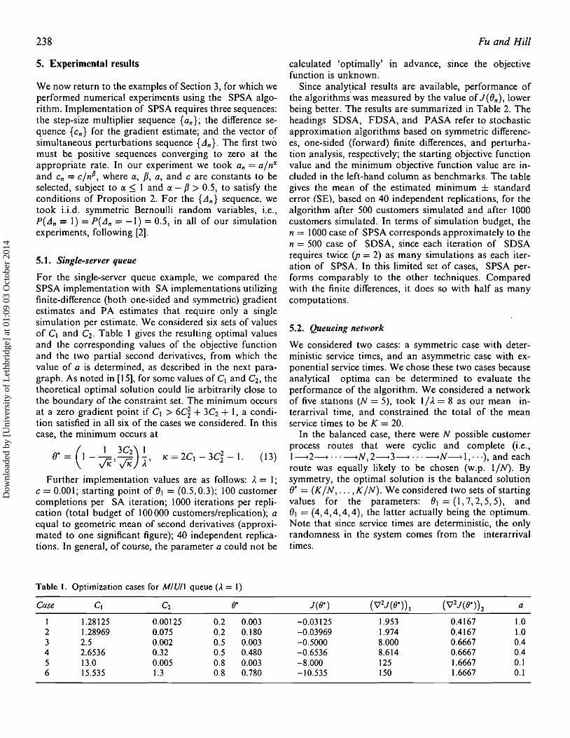
For the single-server queue example, we compared theSPSA implementation with SA implementations utilizingfinite-difference (both one-sided and symmetric) gradientestimates and PA estimates that require only a singlesimulation per estimate. We considered six sets of valuesof C t and C2. Table ] gives the resulting optimal valuesand the corresponding values of the objective functionand the two partial second derivatives, from which thevalue of a is determined, as described in the next para­graph. As noted in [15], for some values of Ct and C2, thetheoretical optimal solution could lie arbitrarily close tothe boundary of the constraint set. The minimum occursat a zero gradient point if C1 > 6C~ + 3C2 + I, a condi­tion satisfied in all six of the cases we considered. In thiscase, the minimum occurs at

calculated 'optimally' in advance, since the objectivefunction is unknown.

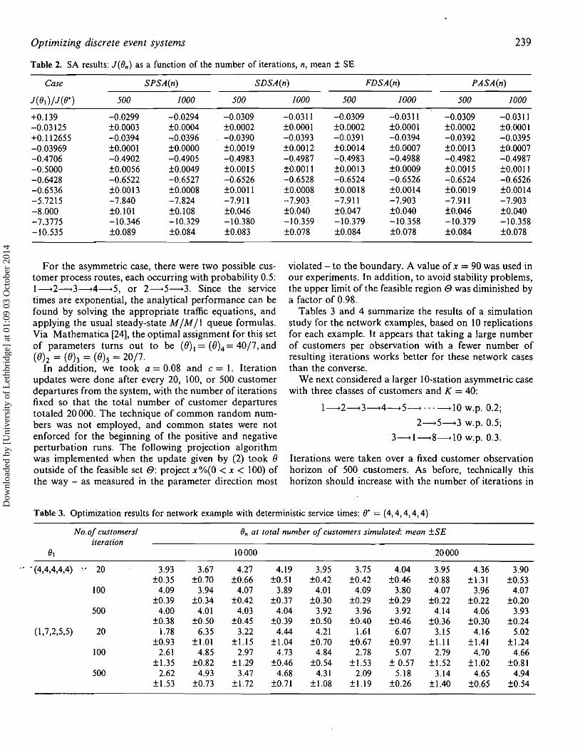
Since analytical results are available, performance ofthe algorithms' was measured by the value of J((Jn), lowerbeing better. The results are summarized in Table 2. Theheadings SDSA, FDSA, and PASA refer to stochasticapproximation algorithms based on symmetric differenc­es, one-sided (forward) finite differences, and perturba­tion analysis, respectively; the starting objective functionvalue and the minimum objective function value are in­cluded in the left-hand column as benchmarks. The tablegives the mean of the estimated minimum ± standarderror (SE), based on 40 independent replications, for thealgorithm after 500 customers simulated and after 1000customers simulated. In terms of simulation budget, then = 1000 case of SPSA corresponds approximately to then = 500 case of SDSA, since each iteration of SDSArequires twice (p = 2) as many simulations as each iter­ation of SPSA. In this limited set of cases, SPSA per­forms comparably to the other techniques. Comparedwith the finite differences, it does so with half as manycomputations.

5.2. Queueing network

We considered two cases: a symmetric case with deter­ministic service times, and an asymmetric case with ex­ponential service times. We chose these two cases becauseanalytical optima can be determined to evaluate theperformance of the algorithm. We considered a networkof five stations (N = 5), took 1I A == 8 as our mean in­terarrival time, and constrained the total of the meanservice times to be K = 20.

In the balanced case, there were N possible customerprocess routes that were cyclic and complete (i.e.,1-----+2---+ ... ---+N 2--+3---+ ... ---+N---+ I ...) and each, , ,route was equally likely to be chosen (w.p. liN). Bysymmetry, the optimal soJution is the balanced solution(J$ = (KIN, ... l KIN). We considered two sets of startingvalues for the parameters: (Jt = (1,7,2,5,5), and81 = (4,4,4,4,4), the latter actually being the optimum.Note that since service times are deterministic, the onlyrandomness in the system comes from the interarrivaltimes.

(13)O• = (1 - _I 3C2) ~ 2C 3C2 1V'K'.jK A' K= 1- 2-'

Table t. Optimization cases for MIU/l queue (A = 1)

Case Ct C2 O· J((r) (V2J (O· )) t (V2J (O*))2 a

1 1.28125 0.00125 0.2 0.003 -0.03125 1.953 0.4167 1.02 1.28969 0.075 0.2 0.180 -0.03969 1.974 0.4167 1.03 2.5 0.002 0.5 0.003 -0.5000 8.000 0.6667 0.44 2.6536 0.32 0.5 0.480 -0.6536 8.614 0.6667 0.45 13.0 0.005 0.8 0.003 -8.000 125 1.6667 0.16 15.535 1.3 0.8 0.780 -10.535 150 1.6667 0.1

Dow

nloa

ded

by [

Uni

vers

ity o

f L

ethb

ridg

e] a

t 01:

09 0

3 O

ctob

er 2

014

Optimizing discrete event systems 239

Table 2. SA results: J{On) as a function of the number of iterations, n, mean ± SE

Case SPSA(n) SDSA(n) FDSA(n) PASA (n)

J (0.) /J (e:) 500 1000 500 1000 500 1000 500 1000

+0.139 -0.0299 -0.0294 -0.0309 -0.0311 -0.0309 -0.0311 -0.0309 -0.0311-0.03125 to.OOO3 ±0.0004 to.OO02 to.OOOI to.OOO2 to.OOOI to.0002 fO.OOOI+0.112655 -0.0394 -:0.0396 -0.0390 -0.0393 -0.0391 -0.0394 -0.0392 -0.0395-0.03969 to.OOOl to.OOOO ±0.0019 to.0012 to.OO14 to.OOO7 to.OOI3 to.0007-0.4706 -0.4902 -0.4905 -0.4983 -0.4987 -0.4983 -0.4988 -0.4982 -0.4987-0.5000 to.0056 ±0.0049 to.0015 to.OOll to.0013 to.0009 to.0015 to.OOl J

-0.6428 -0.6522 -0.6527 -0.6526 -0.6528 -0.6524 -0.6526 -0.6524 -0.6526-0.6536 to.OO13 to.OO08 fO.OOll to.0008 to.0018 to.OO14 to.OOI9 to.0014-5.7215 -7.840 -7.824 -7.911 -7.903 -7.911 -7.903 -7.911 -7.903-8.000 ±O.lOl to.108 ±0.046 to.040 to.047 ±O.040 to.046 to.040-7.3775 -10.346 -10.329 -10.380 -10.359 -10.379 -10.358 -10.379 -10.358-10.535 to.089 ±0.084 to.083 ±0.078 ±O.084 to.078 to.084 to.078

For the asymmetric case, there were two possible cus­tomer process routes, each occurring with probability 0.5:l---+2~3~4~5, or 2~5---+3. Since the servicetimes are exponential, the analytical performance can befound by solving the appropriate traffic equations, andapplying the usual steady-state M / M /1 queue formulas.Via Mathematica [24], the optimal assignment for this setof parameters turns out to be (8)1= {(})4 = 40/7, and(8)2 = (Oh = (8)5 = 20/7.

In addition, we took a = 0.08 and c = 1. Iterationupdates were done after every 20, 100, or 500 customerdepartures from the system, with the number of iterationsfixed so that the total number of customer departurestotaled 20000. The technique of common random num­bers was not employed, and common states were notenforced for the beginning of the positive and negativeperturbation runs. The folJowing projection algorithmwas implemented when the update given by (2) took 8outside of the feasible set 8: project X 0/0(0 < x < 100) ofthe way - as measured in the parameter direction most

violated - to the boundary. A value of x = 90 was used inour experiments. In addition, to avoid stability problems,the upper limit of the feasible region e was diminished bya factor of 0.98.

Tables 3 and 4 summarize the results of a simulationstudy for the network examples, based on 10 replicationsfor each example. It appears that taking a large numberof customers per observation with a fewer number ofresulting iterations works better for these network casesthan the converse.

We next considered a larger l O-station asymmetric casewith three classes of customers and K = 40:

I---t2~3---+4---+5~··· ~lO w.p. 0.2;

2---+5---+3 w.p, 0.5;

3---+1---+8---+10 w.p. 0.3.

Iterations were taken over a fixed customer observationhorizon of 500 customers. As before, technically thishorizon should increase with the number of iterations in

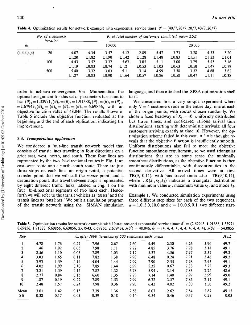
Table 3. Optimization results for network example with deterministic service times: 0" = (4,4,4,4,4)

No.of customers! ()" at total number of customers simulated: mean ±SEiteration

01 10000 20000

., - (4,4,4,4,4) 'f 20 3.93 3.67 4.27 4.19 3.95 3.75 4.04 3.95 4.36 3.90to.35 ±0.70 to.66 to.51 to.42 fO.42 to.46 to.88 tl.31 ±0.53

100 4.09 3.94 4.07 3.89 4.01 4.09 3.80 4.07 3.96 4.07±0.39 to.34 ±0.42 fO.37 fO.30 ±0.29 to.29 fO.22 ±0.22 to.20

500 4.00 4.01 4.03 4.04 3.92 3.96 3.92 4.14 4.06 3.93to.38 fO.50 ±0.45 ±O.39 to.50 to.40 ±0.46 ±O.36 to.30 fO.24

(1,7,2,5,5) 20 1.78 6.35 3.22 4.44 4.21 1.61 6.07 3.15 4.16 5.02to.93 tl.OI ±1.15 ±1.04 fO.70 ±O.67 ±0.97 fl.ll tt.41 ±1.24

100 2.61 4.85 2.97 4.73 4.84 2.78 5.07 2.79 4.70 4.66±1.35 ±0.82 f1.29 to.46 to.54 ±1.53 ± 0.57 ±1.52 ±1.02 to.81

500 2.62 4.93 3.47 4.68 4.31 2.09 5.18 3.14 4.65 4.94t1.53 fO.73 fl.72 fO.7l t1.08 ±1.19 to.26 t1.40 to.65 to.54

Dow

nloa

ded

by [

Uni

vers

ity o

f L

ethb

ridg

e] a

t 01:

09 0

3 O

ctob

er 2

014

240 Fu and Hill

Table 4. Optimization results for network example with exponential service times: (t = (40/7 ,20/7,20/7,40/7,20/7)

No. of customersl On at total number of customers simulated: mean ±SEiteration

(}I ]0000 20000

(4,4,4,4,4) 20 4.07 4.34 3.57 5.12 2.89 5.47 3.73 3.28 4.33 3.20tl.20 ±1.82 ±I.90 ±1.42 ±1.28 ±1.48 ±0.83 ±1.51 ±1.23 ±1.01

100 4.43 3.52 3.37 5.63 3.05 5.11 3.00 3.29 5.43 3.16±1.19 ±0.83 ±O.74 ±1.2} ±0.53 tl.03 ±O.63 to.50 ±1.47 ±0.79

500 5.40 3.32 3.03 5.11 3.14 4.99 3.38 3.32 4.68 3.62±1.27 to.83 ±0.90 ±1.64 ±0.57 ±0.86 ±0.58 to.47 ±l.] I ±0.38

Example 1. We conducted simulation experiments usingthree different step sizes for each of the two sequences:a = 1.0,3.0, 10.0 and c = 1.0,0.5,0.1; two different start-

language, and then attached the SPSA optimization shellto it.

We considered first a very simple experiment whereonly N = 4 customers rode in the entire day, one at eachof the origin points, with routes chosen randomly. Wechose a fixed headway of K; = 10, uniformly distributedbus travel times, and considered various arrival timedistributions, starting with deterministic arrivals: all fourcustomers arriving exactly at time 10. However, the op-timization scheme failed in this case. A little thought re­

5.3. Transportation application\ veals that the objective function is insufficiently smooth.

We considered a four-line transit network model that Uniform distributions also fail to meet the objectiveconsists of transit lines traveling in four directions on a function smoothness requirement, so we used triangulargrid: east, west, north, and south. These four lines are distributions that are in some sense the minimaJlyrepresented by the two bi-directional routes in Fig. 1: an smoothest distributions, as the objective function is theneast-west route and a north-south route. There are just continuously differentiable, with discontinuities in thethree stops on each line: an origin point, a potential second derivative. All arrival times were at timetransfer point that we will call the center point, and a TR(9,IO,II), with bus travel times also TR(9JO,11),destination point. Bus travel between stops is represented where TR(kl , k2 , k3) indicates a triangular distributionby eight different traffic 'links' labeled in Fig. 1 on the with minimum value k), maximum value k3, and mode k2.four bi-directional segments of two links each. Hence­forth we will refer to the transit vehicles as 'buses' and thetransit lines as 'bus lines.' We built a simulation programof the transit network using the SIMAN simulation

order to achieve convergence. Via Mathematica, theoptimal assignment for this set of parameters turns out tobe: (Oh= 1.33971, (O)2=(B)s= 1.91388, (8)1 =(8)8=(8)10=2.67943, (8)4 = (8)6 = (0)7 = (8)9 = 6.69856, with anobjective function value of 48.046. The results shown inTable 5 include the objective function evaluated at thebeginning and the end of each replication, indicating theimprovement.

Table 5. Optimization results for network example with 10 stations and exponential service times: 0* = (2.67943, 1.91388, 1.33971,6.69856, 1.91388,6.69856,6.69856,2.67943,6.69856, 2.67943). J((l) = 48.046. (JI = (4.4,4,4,4,4.4.4.4.4). J((J!) = 54.0855

Rep. en after 1000 iterations of 500 customers each: mean J(8n)

I 4.78 1.76 0.27 7.96 2.67 7.60 4.49 2.30 4.26 3.90 49.72 1.46 1.92 0.05 7.98 1.11 7.72 4.85 3.76 7.98 3.18 49.13 2.56 1.10 0.03 7.89 1.03 7.12 5.37 4.56 7.97 2.37 49.24 3.03 1.65 0.11 7.82 1.38 7.93 6.48 0.24 7.91 3.46 49.25 3.93 1.59 0.14 4.04 1.44 7.99 7.90 2.55 7.98 2.43 49.16 4.02 1.99 0.10 7.89 1.44 6.99 5.35 0.67 7.83 3.73 49.37 3.21 1.59 0.15 7.82 1.32 6.78 5.94 . 3.14 7.83 2.22 48.68 2.77 0.84 0.15 6.60 1.35 7.79 7.14 1.40 7.97 3.99 49.09 1.87 0.19 0.22 7.89 1.53 7.99 6.72 3.57 7.85 2.17 49.1

10 2.48 1.57 0.24 7.98 0.36 7.92 6.42 4.02 7.80 1.20 49.2

Mean 3.01 1.42 0.15 7.39 1.36 7.58 6.07 2.62 7.54 2.87 49.15SE 0.32 0.17 0.03 0.39 0.18 0.14 0.34 0.46 0.37 0.29 0.03

Dow

nloa

ded

by [

Uni

vers

ity o

f L

ethb

ridg

e] a

t 01:

09 0

3 O

ctob

er 2

014

Optimizing discrete event systems

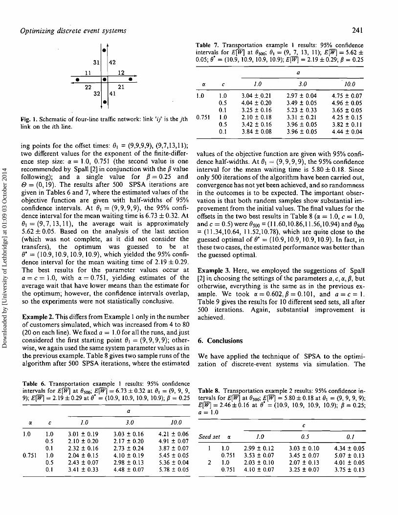
•31 42

11 12

• • •22 21

32 41

•Fig. 1. Schematic of four-line traffic network: link 'i]' is the jthlink on the itb line.

ing points for the offset times: 81 = (9,9,9,9), (9,7,13,11);two different values for the exponent of the finite-differ­ence step size: a. = 1.0, 0.751 (the second value is onerecommended by Spall [2] in conjunction with the f3 valuefollowing); and a single value for f3 = 0.25 ande = (0,19). The results after 500 SPSA iterations aregiven in Tables 6 and 7, where the estimated values of theobjective function are given with half-widths of 95%confidence intervals. At (JI = (9,9,9,9), the 950/0 confi­dence interval for the mean waiting time is 6.73 ± 0.32. At01 = (9,7,13,11), the average wait is approximately5.62 ± 0.05. Based on the analysis of the last section(which was not complete, as it did not consider thetransfers), the optimum was guessed to be at8· = (10.9,10.9,10.9,10.9), which yielded the 95% confi­dence interval for the mean waiting time of 2.19 ± 0.29.The best results for the parameter values occur atQ = C = 1.0, with a = 0.751, yielding estimates of theaverage wait that have lower means than the estimate forthe optimum; however, the confidence intervals overlap,so the experiments were not statistically conclusive.

Example 2. This differs from Example 1 only in the numberof customers simulated, which was increased from 4 to 80(20 on each line). We fixed Q = 1.0 for all the runs, andjustconsidered the first starting point (JI = (9,9) 9, 9); other­wise, we again used the same system parameter values as inthe previous example. Table 8 gives two sample runs of thealgorithm after 500 SPSA iterations, where the estimated

241

Table 7. Transportation example 1 results: 95% confidenceintervals for E[W] at 8500 ; 81 = (9, 7, 13, 11); E[W] = 5.62 ±0.05; 8· = (l0.9, 10.9, 10.9,10.9); EfW] = 2.19 ± 0.29; P= 0.25

a

ex c 1.0 3.0 10.0

1.0 1.0 3.04 ±.D.21 2.97 ± 0.04 4.75 ± 0.070.5 4.04 ± 0.20 3.49 ± 0.05 4.96 ± 0.050.1 3.25 ± 0.16 5.23 ± 0.33 3.65 ± 0.05

0.751 1.0 2.10 ± 0.18 3.31 ± 0.21 4.25±0.150.5 3.42 ± 0.16 3.96 ± 0.05 3.82 ± 0.110.1 3.84 ± 0.08 3.96 ± 0.05 4.44 ± 0.04

values of the objective function are given with 950/0 confi­dence half-widths. At B1 == (9,9,9,9), the 95% confidenceinterval for the mean waiting time is 5.80 ± 0.18. Sinceonly 500 iterations of the algorithm have been carried out,convergence has not yet been achieved, and so randomnessin the outcomes is to be expected. The important obser­vation is that both random samples show substantial im­provement from the initial values. The final values for theoffsets in the two best results in Table 8 (ex = 1.0, c = 1.0,and c = 0.5) were 8500 = (11.60,10.86,11.56,10.94) and 8500= (11.34,10.64, 11.52,10.78), which are quite close to theguessed optimal of O· = (10.9,10.9,10.9,10.9). In fact, inthese two cases, the estimated performance was better thanthe guessed optimal.

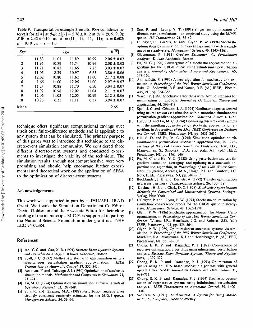
Example 3. Here, we employed the suggestions of Spall[2] in choosing the settings of the parameters Q, C, (J., {3, butotherwise, everything is the same as in the previous ex­ample. We took ex = 0.602, P= 0.101) and Q = C = 1.Table 9 gives the results for 10 different seed sets, all after500 iterations. Again, substantial improvement isachieved.

6. Conclusions

We have applied the technique of SPSA to the optimi­zation of discrete-event systems via simulation. The

Table 6. Transportation example 1 results: 950/0 confidenceintervals for EfW] at 8500 ; EfW] = 6.73 ± 0.32 at 81 = (9, 9, 9,9); E[W] = 2.19 ± 0.29 at 8· = (l0.9, 10.9, 10.9, 10.9); P= 0.25

a

lX C 1.0 3.0

1.0 1.0 3.01 ±0.19 3.03 ± 0.160.5 2.10 ± 0.20 2.17 ± 0.200.1 2.32±0.16 2.73 ± 0.24

0.751 1.0 2.04 ± 0.15 4.10 ± 0.190.5 2.43 ± 0.07 2.98 ± 0.130.1 3.41 ± 0.33 4.48 ± 0.07

Table 8. Transportation example 2 results: 950/0 confidence in­tervals for E[W] at 8500 ; E[W] = 5.80 ± O.l~ at 81 = (9, 9, 9, 9);E[W] = 2.46 ± 0.16 at 8· = (10.9, 10.9, 10.9, 10.9); f3 = 0.25;a = 1.0

10.0 c

4.21 ± 0.06 Seed set lX 1.0 0.5 0.14.91 ± 0.073.87 ± 0.07 1.0 2.99 ± 0.12 3.03 ± 0.10 4.34 ± 0.055.45 ± 0.05 0.751 3.53 ± 0.07 3.45 ± 0.07 5.07 ± 0.135.36 ± 0.04 2 1.0 2.03 ± 0.10 2.07 ± 0.13 4.01 ± 0.055.78 ± 0.05 0.751 4.10 ± 0.07 3.25 ± 0.07 3.75 ± 0.13

Dow

nloa

ded

by [

Uni

vers

ity o

f L

ethb

ridg

e] a

t 01:

09 0

3 O

ctob

er 2

014

242

Table 9. Transportation example 3 results: 95% confidence in-tervals for E[W] at 8500; E[W] = 5.76 ± 0.12 at 81 = (9, 9, 9, 9);E[WJ = 2.45 ± 0.10 at 8- = (l l , II, II, II); (X = 0.602;P=O.IOl;a=c=l.O

Rep. 8500 Erw]

I 11.83 11.01 11.89 10.99 2.06 ± 0.072 11.95 10.89 11.74 10.96 2.08 ± 0.083 11.21 10.83 11.65 7.25 3.03 ± 0.074 11.05 8.29 ]0.97 6.63 3.86 ± 0.065 12.02 10.80 11.62 11.00 2.17 ± 0.086 1.66 11.00 12.06 11.00 2.07 ± 0_077 J1.24 10.88 11.70 6.50 3.04 ± 0.078 1J.92 10.98 12.02 11.04 2.J 1 ± 0.079 12.06 11.03 12.05 10.99 2.J2 ± 0.06

10 10.93 6.35 11.11 6.57 3.94 ± 0.07

Mean 2.65

technique offers significant computational savings overtraditional finite-difference methods and is applicable toany system that can be simulated. The primary purposeof this paper was to introduce this technique to the dis­crete-event simulation community. We considered threedifferent discrete-event systems and conducted experi­ments to investigate the viability of the technique. Thesimulation results, though not comprehensive, were verypromising and should help encourage further experi­mental and theoretical work on the application of SPSAto the optimization of discrete-event systems.

Acknowledgements

This work was supported in part by a JHU/APL IRADGrant. We thank the Simulation Department Co-EditorDavid Goldsman and the Associate Editor for their closereading of the manuscript. M.e.F. is supported in part bythe National Science Foundation under grant no. NSFEEe 94-02384.

References

[I] HOt Y. C. and Cao, X. R. (1991) Discrete Event Dynamic Systemsand Perturbation Analysis, Kluwer Academic, Boston.

[2] Spall, J. C. (1992) Multivariate stochastic approximation using asimultaneous perturbation gradient approximation. IEEETransactions on Automatic Control, 37, 332-341.

[3] Azadivar, F. and Talavage, 1.1. (1980) Optimization of stochasticsimulation models. Mathematics and Computers in Simulation, 22,23 ]-241.

[4] Fu, M. C. (1994) Optimization via simulation: a review. Annals ofOperations Research. 53, 199-248.

[5] Suri, R. and Zazanis, M.A. (1988) Perturbation analysis givesstrongly consistent sensitivity estimates for the M/GIl queue.Management Science, 34. 39-64.

Fu and Hill

[6] Suri, R. and Leung, Y. T. (1991) Single run opnrmzauon ofdiscrete event simulations - an empirical study using the MIMI]queue. lIE Transactions, 21, 35-49.

[7] L'Ecuyer, P., GIroux, N. and Glynn, P. W. (1994) Stochasticoptimizauon by simulation: numerical experiments with a simplequeue in steady-state. Management Science, 40, ]245-1261.

[8] Glasserman, P. (1991) Gradient Esumatton Vw PerturbationAnalysis, Kluwer Academic, Boston.

[9] Fu, M. C. (1990) Convergence of a stochastic approximation al­gorithm for the GIlG/I queue using infinitesimal perturbationanalysis. Journal of Optimization Theory and Applicattons. 65,149-160.

[10] Andradottir, S. (1990) A new algorithm for stochastic approxi­mation, 10 Proceedings of the 1990 Wznter Simulation Conference,Bald, 0., Sadowski, R.P. and Nance, R.E. (00.) IEEE, Piscata­way, NJ, pp. 364-366.

[I]] Wardi, Y. (1990) Stochastic algorithms with Armijo stepsizes formimrruzatron of functions. Journal of Optimization Theory andApplications, 64, 399-418.

[12] Spall, 1. C. and Cristion, J. A. (1994) Nonlinear adaptive controlusing neural networks: estimation with a smoothed simultaneousperturbation gradient approximation. Statistica Sinica, 4, 1-27.

[13] HllJ, S. D. and Fu, M. C. (1994) Opumizmg discrete event systemswith the Simultaneous perturbation stochastic approximation alagorithm, in Proceedings of the 33rd IEEE Conference on Decisionand Control, IEEE, Piscataway, NJ, pp. 263]-2632.

[14] Hill, S. D. and Fu, M. C. (1994) Simulation optimization viasimultaneous perturbation stochastic approximation, in Pro­ceedings of the 1994 Winter Simulation Conference, Tew, J.D.,Manivannan, S., Sadowski, D.A. and Seila, A.F. (ed.) IEEE,Piscataway, NI, pp. 146]-1464.

[15] Fu, M_ C_ and Ho, Y. C. (1988) Using perturbation analysis forgradient estimation, averaging, and updating 10 a stochastic ap­proximation algonthm, In Proceedings of the 1988 Wmter Simu­lation Conference, Abrams, M.A., Haigh, P.L. and Comfort. J.C.(ed.), IEEE, Piscataway, Nl, pp. 509-5]7.

[16] Bookbinder, J. H. and Desilets, A. (1992) Transfer optimizationin a transit network. Transportation Science, 26, 106-118.

[17] Kushner, H. J. and Clark, D. C. (1978) Stochastic ApproximationMethods for Constrained and Unconstrained Systems, Springer-Verlag, New York. '

[18] L'Ecuyer, P. and Glynn, P. W. (1994) Stochasuc optimization bysimulation: convergence proofs for the GIlG/l queue in steady­state. Management Science, 40, 1562-1578.

[19] Glynn, P. W. (1986) Stochastic approximation for Monte Carloopurmzation, in Proceedings of the 1986 l-Vmter Stmulatton Con­ference, Wilson, 1.R., Henriksen, 1.0. and Roberts, S.D. (ed.)IEEE, Piscataway, NJ, pp. 356-364.

[20] Glynn, P. W. (1989) Optimization 'of stochastic systems via sim­ulation, in Proceedings of the 1989 Winter Simulation Conference,MacNarr, E.A., Musselman, K.J. and Heidelberger, P. (ed.) IEEE,Piscataway, NJ, pp. 90-105.

[21] Chong, E. K. P. and Ramadge, P. 1. (1992) Convergence ofrecursive optimization algonthms usmg infinitesimal perturbationanalysis. Discrete Event Dynamic Systems: Theory and Applica­tions, I, 339-372.

[22] Chong, E. K P and Ramadge, P J. (1993) Optimization ofqueues using an IPA based stochastic algorithm with generalupdate umes. SIAM Journal on Control and Optimtzatton, 31.698-732.

[23] Chong, E. K. P. and Ramadge, P. J. (1994) Stochastic opurru­zation of regenerative systems using infinitesimal perturbationanalysis. IEEE Transactions on Automatic Control. 39, 1400­1410.

[24] Wolfram, S. (1991) Mathematica: A System for Doing Mathe­matics by Computer, Addison-Wesley.

Dow

nloa

ded

by [

Uni

vers

ity o

f L

ethb

ridg

e] a

t 01:

09 0

3 O

ctob

er 2

014

Optimizing discrete event systems

Biographies

Michael C. Fu is an Associate Proffessor of Management Science &Statistics in the College of Business and Management, with a jointappointment in the Institute for Systems Research, at the University ofMaryland at College Park. He received a bachelor's degree in mathe­matics and bachelor's and master's degrees in electrical engineeringfrom MIT in 1985, and M.S. and Ph:D. degrees in applied mathe­matics from Harvard University in 1986 and 1989, respectively. Hisresearch interests include simulation optimization and sensitivityanalysis, particularly with applications towards manufacturing sys­tems, inventory control, and the pricing of financial derivatives. Heteaches courses in applied probability, stochastic processes, discrete­event simulation, and operations management, and in 1995 wasawarded the Allen J. Krowe Award for Teaching Excellence. Heserved on the Program Committee for the Spring 1996 INFORMS

243

National Meeting and is on the Editorial Boards of lIE Transactionsand INFORMS Journal on Computing.

Stacy D. Hill is a Systems Engineer on the Senior Professional Staff ofthe Johns Hopkins University Applied Physics Laboratory. He re­ceived the B.S. and M.S. degrees from Howard University in 1975 and1977, respectively, and the D.Sc. degree in control systems engineeringand applied mathematics from Washington University in 1983. He hasbeen project and technical lead in developing, testing, and applyingstatistical estimation techniques and software, and has authored andco-authored journal articles on estimation theory and techniques, in­cluding an article in the cross-disciplinary book Bayesian Analysis ofTime Series and Dynamic Models. His present research interests includeoptimization and simulation of discrete event systems, with applicationto transportation problems.

Dow

nloa

ded

by [

Uni

vers

ity o

f L

ethb

ridg

e] a

t 01:

09 0

3 O

ctob

er 2

014