1

c-SPSA: Cluster-wise Simultaneous Perturbation Stochastic Approximation Algorithm and its Application to Dynamic Origin-

Destination Matrix Estimation Athina Tympakianaki a*, Haris N. Koutsopoulos ab, Erik Jenelius a

aDepartment of Transport Science, KTH Royal Institute of Technology,

SE-100 44 Stockholm, Sweden bDepartment of Civil and Environmental Engineering, Northeastern University

Boston, MA 02115

* Corresponding author. Tel.: +46 8 7908891. Email addresses: athinat@kth.se (A. Tympakianaki), hnk@kth.se (H.N. Koutsopoulos),

jenelius@kth.se (E. Jenelius) Abstract: The Simultaneous Perturbation Stochastic Approximation (SPSA) algorithm has been used in the literature for the solution of the dynamic origin-destination (OD) estimation problem. Its main advantage is that it allows quite general formulations of the problem that can include a wide range of sensor measurements. While SPSA is relatively simple to implement, its performance depends on a set of parameters that need to be properly determined. As a result, especially in cases where the gradient of the objective function changes quickly, SPSA may not be as stable and even diverge. A modification of the SPSA algorithm, referred to as c-SPSA, is proposed which applies the simultaneous perturbation approximation of the gradient within a small number of carefully constructed “homogeneous” clusters one at a time, as opposed to all elements at once. The paper establishes the theoretical properties of the new algorithm with an upper bound for the bias of the gradient estimate and shows that it is lower than the corresponding SPSA bias. It also proposes a systematic approach, based on the k-means algorithm, to identify appropriate clusters. The performance of c-SPSA, with alternative implementation strategies, is evaluated in the context of estimating OD flows in an actual urban network. The results demonstrate the efficiency of the proposed c-SPSA algorithm in finding better OD estimates and achieve faster convergence and more robust performance compared to SPSA with fewer overall number of function evaluations. Keywords: SPSA; Origin-Destination (OD) matrix estimation; stochastic approximation; k-means clustering; gradient estimation bias.

1. Introduction

Estimation of time-dependent Origin-Destination (OD) flows is important since they are essential input to a number of applications where the spatial and temporal distribution of travel demand for a specific transportation network is of interest. Dynamic traffic assignment (DTA) models, for example, use OD flows as a main input, along with various parameters that capture the performance of the network (e.g. capacities and speed-density relationships) and the travel behavior of travelers and assign them onto a network.

2

OD matrices are difficult and expensive to obtain directly, and for this reason they are often estimated using indirect measurements such as traffic counts. The general OD matrix estimation problem is thus to find an OD flow vector that best matches a set of indirect observations (e.g. counts and speeds at sensor locations and point-to-point travel times). The problem can be formulated as an optimization problem as follows: Min , , (1) subject to 0 where , are functions that measure the “distance” between the estimated quantities from their observed values. They also incorporate weights that capture the uncertainty in the observations and the accuracy of the seed OD matrix. is the unknown time-dependent OD flow vector, a historic (seed) OD vector, a set of observations, and the corresponding set of observations predicted by a model after has been assigned to the network. The OD estimation problem has been thoroughly addressed in the literature and different solution approaches have been proposed (see Cantelmo et al., 2014 for a brief review). The proposed approaches can be categorized as assignment matrix-based and assignment matrix-free methods. The assignment matrix is a (linear) mapping of the unknown OD flows to link traffic counts, i.e. . is the assignment matrix expressed as the proportions of OD flows crossing sensor locations over different time intervals (Spiess, 1990). Assignment matrix-based formulations have the advantage that the gradient of the objective function can be analytically computed, resulting in more efficient and robust solutions (see for example Cascetta and Postorino, 2001; Frederix et al., 2011; Toledo and Kolechkina, 2013). However, the assignment matrix makes the use of data sources other than traffic counts difficult, as their relationship with the unknown OD matrix cannot be easily captured analytically. This limitation is particularly important in light of the emergence of new dedicated and opportunistic sensor technologies that provide data on speeds, travel times, and even trajectories. On the other hand, the assignment matrix-free approaches use a general formulation, which allows for the incorporation of any data sources, e.g. traffic speeds and point-to-point travel times. Recent literature has focused on such general formulations and solution approaches (see for example Balakrishna, 2006; Balakrishna et al., 2007; Balakrishna and Koutsopoulos, 2008; Vaze et al., 2009; Cipriani et al., 2011). In the assignment matrix-free class of methods, due to the complexity of the problem, function in eq. (1) is usually a complex simulation model that receives as input the OD flows and outputs the corresponding observations. The output of the simulation captures indirectly the complex relationship between the OD flows and the available data. Due to the use of simulation to evaluate , the objective function of the OD estimation problem is stochastic and the identification of the solution more complicated. Various researchers (e.g. Balakrishna et. al., 2008, Cipriani et. al., 2011) have used the simultaneous perturbation stochastic approximation (SPSA) algorithm (Spall, 1998; 1999; 2003) for the solution of the problem. Although SPSA is relatively simple to implement, it has a number of disadvantages

3

and limitations. Its performance is sensitive to the selection of the initial algorithmic parameters, the scale of the variables, and the shape of the objective function and associated gradient. The algorithm (depending on the choice of the step size for updating the solution and other parameters) may be very slow or even diverge if the function is steep. The objective of this paper is to propose a modified SPSA algorithm in order to overcome some of the documented limitations of the original SPSA and improve its convergence and stability. The main idea of the modified algorithm is the clustering of the unknown variables (e.g. the components of the OD flow matrix) into a small number of “homogeneous” clusters (based for example on their initial values). The main difference compared to SPSA regards the gradient approximation approach employed by the two algorithms. In the proposed algorithm the gradient is approximated separately for OD pairs belonging to a specific cluster by perturbing the flows only for those OD pairs, whereas in the SPSA algorithm the gradient is approximated for all the OD pairs simultaneously. The proposed algorithm is referred as cluster-based SPSA (c-SPSA). The paper establishes the theoretical properties of c-SPSA showing the reduced bias of the estimated gradient, which is expected to lead to improved stability and efficiency. The paper also suggests a method for clustering of the OD pairs using the k-means clustering algorithm and suitable termination criteria to decide on the appropriate number of clusters. A case study in the context of OD estimation with a realistic network is used to evaluate the performance of the algorithm in terms of its stability, convergence, computational efficiency and solution quality. Different implementation variants of c-SPSA are considered, including adaptive clustering (where the clusters are redefined periodically during the iterations of the algorithm). The impact of factors such as, number of clusters and need for gradient averaging are assessed. The results are very promising, demonstrating that c-SPSA has the potential to not only identify good solutions to the OD estimation problem, but also be more efficient than SPSA in doing so. The remainder of the paper is organized as follows. Section 2 examines the stochastic approximation approach to the solution of the OD estimation problem and discusses the main issues and limitations of stochastic approximation algorithms and their sources. Section 3 introduces the new algorithm, c-SPSA, establishes its theoretical properties, and proposes a k-means approach for the identification of appropriate clusters. Section 4 presents the case study and the experimental design and performance measures used for the evaluation of the proposed algorithm. Section 5 analyses the results and demonstrate that c-SPSA outperforms SPSA in terms of quality of solution, convergence rate, and computational efficiency. Section 6 concludes the paper.

2. Stochastic approximation methods

SPSA belongs to the general class of stochastic approximation (SA) methods used for the solution of optimization problems with noisy objective functions that are usually expensive to evaluate (Spall, 2003). SA methods were first introduced for solving root-finding problems in the presence of noisy function measurements (Robbins and Monro, 1951). Extensions to optimization and multidimensional problems followed (e.g. Blum, 1954, Kiefer and Wolfowitz, 1952).

4

The standard SA approach for optimization problems is based on the following recursion: (2) where is the estimate of the gradient at iteration based on measurements of the objective function, and are positive scalars satisfying three basic conditions: 0∀ , ∑ ∞ and ∑ ∞. Under appropriate conditions, the iterations in (2) converge to ∗ in some stochastic sense. Depending on the availability of the (noisy) gradient the algorithms are categorized as direct gradient-based (direct) or gradient-free (indirect). Of interest to the problem of OD estimation is the indirect gradient methods, since for this class of problems the gradient is not (easily) available. For the indirect gradient case, different algorithms employ various alternatives to estimate the gradient at each iteration, including the Kiefer-Wolfowitz algorithm and the Simultaneous Perturbations approach. 2.1 Kiefer-Wolfowitz algorithm (FDSA) Kiefer and Wolfowitz (1952), in their classic paper, proposed the use of the finite difference (FD) approximation of the gradient. The FD stochastic approximation (FDSA) relies on one-at-a-time perturbations of each element of , at iteration , to estimate the gradient. Two-sided approximations involve measurements of the form perturbation , according to eq. (3).

⋮

(3)

is the dimension of and denotes a vector with 1s in the th location and 0s elsewhere. The

pair , are positive gain sequences. should satisfy the conditions stated in the previous section. should satisfy the following conditions: → 0, ∑ ∞ and ∑ /∞.

2.2 Simultaneous perturbation stochastic approximation algorithm (SPSA)

The disadvantage of FDSA is that it requires 2p function evaluations at each iteration. Therefore, the computational cost can be prohibitive, especially when simulation is used for function evaluation. The simultaneous stochastic perturbation stochastic approximation (SPSA) algorithm, proposed by Spall (1998; 1999; 2003), perturbs all the elements in simultaneously; hence SPSA relies only on two function measurements for the approximation of the gradient of the objective function at each iteration. The two-sided SP approximation in iteration is:

5

∆ ∆

∆∆ ∆

∆

⋮∆ ∆

∆

(4)

where ∆ is a zero-mean -dimensional perturbation vector for the th iteration. The perturbation factor is / ( and are algorithmic parameters). The components of ∆ may be independently generated from a Bernoulli distribution with ±1 values with equal probability. In order to increase the accuracy of the gradient approximation, a common technique is to conduct several gradient replications at each iteration and take the average gradient. Vector is updated using the recursive step in eq. (2). The step size is determined by the sequence / ( and are algorithmic parameters). The selection of the gain sequences and is very critical for the performance of SPSA. Practical guidelines for the selection of the algorithmic parameters , , , and are provided in Spall (2003), and Vaze et al. (2009). 2.3 Discussion The FDSA algorithm is inefficient for large scale problems, such as the OD estimation problem, as the number of objective function evaluations increases directly with the size of the OD matrix. On the other hand, SPSA uses a computationally efficient estimate of the gradient, as it requires only two function evaluations at each iteration. Furthermore, the convergence rate of the two algorithms is similar, as they both reach statistically similar objective function values with the same number of iterations (but in the case of SPSA with much fewer function evaluations). The performance of this class of algorithms can be problematic though, especially if the gradient is steep, i.e. changes faster than linearly with the inputs (Andradóttir 1996). Some of these issues can be addressed by careful choice of the algorithmic parameters that determine sequences , . However, this is not easy and can be very time consuming. For example, if the values of are small the algorithm will move very slowly (especially where the function is flat), while a more aggressive sequence can lead to large step sizes that cause the algorithm to diverge (especially if the current iteration lies at a region where the function is steep). Similarly, while small values of the sequence can reduce the bias of the estimated gradient, they also increase the variance (noise) of the estimate (Broadie et. al., 2011). In any case, proper selection of the algorithmic parameters is critical for its performance (including stability). The algorithmic stability issues are compounded in problem instances where the components of the vector to be optimized vary significantly in magnitude, as the performance of the algorithm depends on the scale of these variables (Spall, 2003).

6

There are different recommendations in the literature for how to deal with some of these issues. Spall (1992), in order to enhance the performance of the SPSA algorithm when the noise in the objective function is high, suggests that the gradient be estimated as the average of a number of independent simultaneous perturbation approximations. Spall (1998) discusses scaling issues and suggests the scaling of the gain sequence , especiallyin cases where the unknown variables vary in magnitude. He later proposed an extension of the standard SPSA algorithm, referred to as adaptive SPSA, which uses the Hessian matrix in a stochastic analogue of the Newton-Raphson method for deterministic optimization (Spall, 2000). The method scales the vector of unknown variables automatically. When SPSA is used for the solution of the OD estimation problem, consistent with the above findings, experience shows that approximated gradient values can become extremely noisy and high, which makes it difficult for the algorithm to converge to a good solution and also identify proper algorithmic parameters to improve its stability. The range of possible values of the OD flows (which can be significant for realistic networks ranging from a few vehicles per time interval for some OD pairs to hundreds of vehicles for the main OD pairs) contributes to the problem. Different authors have approached these issues more specifically as they relate to the application of SPSA to the OD problem in different ways. However, no consistent treatment has emerged. Balakrishna et. al. (2007) used a scaling of the ck parameter, based on the magnitude of the corresponding values of the OD flows, to avoid high gradient values. The approach resulted in greater stability, although the treatment is not entirely consistent with the theory. Cipriani et al. (2011) used a modification of the basic SPSA algorithm, assuming a starting OD matrix close to the solution. They introduce a constraint with respect to the total demand generated from any zone in the study area. They also used several gradient replications to estimate the gradient which was approximated using forward (asymmetric) differences. However, although forward differencing can reduce the number of function evaluations it increases the bias of the estimated gradient compared to the central differences method. Subsequently, Cipriani et al. (2014) used the approach to evaluate the impact of different data sources on the accuracy of the dynamic OD matrix estimation. Cipriani et al. (2013) conducted a sensitivity analysis of various implementations aspects of SPSA. In particular, they investigated different values for the perturbation parameter , number of gradient replications, and gradient smoothing (average over a number of iterations, Spall; 2000). The main findings of this work suggest that scaling should be properly chosen as it depends on the shape of the objective function, a rather high number of gradient replications is needed, and that gradient smoothing was not effective.

3. Cluster-based SPSA (c-SPSA)

In this paper a generalization of the original algorithm is proposed in order to deal with the above issues of SPSA on a consistent basis. Specifically, the proposed algorithm, referred to as the cluster-based SPSA (c-SPSA), is a hybrid between the FDSA and SPSA algorithms. c-SPSA makes use of perturbations of the estimated vector at every iteration , similarly to SPSA. However, the elements of are clustered into a small number of “homogeneous” clusters and the gradient is estimated based on a simultaneous perturbation of the sub-vector of that belongs to

7

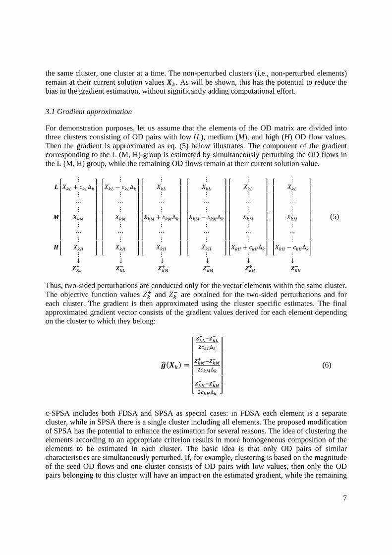
the same cluster, one cluster at a time. The non-perturbed clusters (i.e., non-perturbed elements) remain at their current solution values . As will be shown, this has the potential to reduce the bias in the gradient estimation, without significantly adding computational effort.

3.1 Gradient approximation

For demonstration purposes, let us assume that the elements of the OD matrix are divided into three clusters consisting of OD pairs with low (L), medium (M), and high (H) OD flow values. Then the gradient is approximated as eq. (5) below illustrates. The component of the gradient corresponding to the L (M, H) group is estimated by simultaneously perturbing the OD flows in the L (M, H) group, while the remaining OD flows remain at their current solution value.

⋮∆

⋮⋯⋮

⋮⋯⋮

⋮

⋮∆

⋮⋯⋮

⋮⋯⋮

⋮

⋮

⋮⋯⋮

∆⋮⋯⋮

⋮

⋮

⋮⋯⋮

∆⋮⋯⋮

⋮

⋮

⋮⋯⋮

⋮⋯⋮

∆⋮

⋮

⋮⋯⋮

⋮⋯⋮

∆⋮

(5)

↓↓↓↓↓↓ Thus, two-sided perturbations are conducted only for the vector elements within the same cluster. The objective function values and are obtained for the two-sided perturbations and for each cluster. The gradient is then approximated using the cluster specific estimates. The final approximated gradient vector consists of the gradient values derived for each element depending on the cluster to which they belong:

∆

∆

∆

(6)

c-SPSA includes both FDSA and SPSA as special cases: in FDSA each element is a separate cluster, while in SPSA there is a single cluster including all elements. The proposed modification of SPSA has the potential to enhance the estimation for several reasons. The idea of clustering the elements according to an appropriate criterion results in more homogeneous composition of the elements to be estimated in each cluster. The basic idea is that only OD pairs of similar characteristics are simultaneously perturbed. If, for example, clustering is based on the magnitude of the seed OD flows and one cluster consists of OD pairs with low values, then only the OD pairs belonging to this cluster will have an impact on the estimated gradient, while the remaining

8

OD pairs remain unchanged at their current values, which may result in less noisy and less biased gradient approximation. Additionally, the proposed method allows for the selection of cluster-specific perturbation and step size parameters , , appropriate for the magnitude of the elements within the corresponding cluster.

3.2 Bias in gradient estimation

An interesting question is the impact of the clustering in the bias of the estimated gradient, ≡ | , where is the true gradient at iteration . The gradient

bias for the c-SPSA algorithm can be estimated following an approach analogous to the analysis of the bias of FDSA and SPSA by Spall (2003). For FDSA, the bias of element 1,… , of the gradient vector at iteration is given by

, (7)

where denotes points on the two line segments between and , and represents the third derivative of the objective function with respect to the element of .

Equation (7) implies that has a bias of . Assuming that for all 1,… , , where is a positive constant, the upper bound for this bias is:

| | . (8)

For SPSA the bias of element of the gradient vector, for 1,… , , can be analyzed using the third-order Taylor’s theorem and is given by (Spall, 2003)

∆ ∆ ⨂∆ ⨂∆ , (9)

denotes points on the two line segments between and ∆ , the 1 vector of all possible third derivatives of , ⨂ is the Kronecker product and

, , … , ; ∆ , ∆ , … , ∆ for 1. Assuming that |∆ | , |1/∆ | , and

, where are positive constants and is the element representing the

third derivative of with respect to the , , and elements of ( 1, 2, … , , the bias is bounded by:

| | 1 1 , (10)

For c-SPSA with clusters, the gradient vector consists of components, where each component corresponds to the approximated gradient of a cluster. These sub-gradients are independently calculated (since each element of belongs to one and only one cluster). Applying the same approach as in the estimation of the SPSA bias, but within each cluster separately, it follows that (in the case of c-SPSA) the bias of the estimate for gradient element of a given cluster is bounded by:

9

| | 1 1 . (11)

Where, is the size of cluster , and element ∈ 1,2,… , . Based on (11), which applies for a given cluster, an upper bound on the bias across all gradient elements is obtained by considering the size of the largest cluster, , i.e.,

| | 1 1 (12)

When M = 1 (i.e. p clusters which is the case of FDSA) eq. (12) collapses to (8), the bias upper bound for the FDSA case, as expected. When M = p (i.e. only 1 cluster which is the case of the standard SPSA algorithm) eq. (12) collapses to (10). The important observation is that this upper bound in eq. (12), assuming that the number of clusters is more than one ( 1 , is smaller than the bias of SPSA. More generally, if the components of ∆ are independently generated from a Bernoulli distribution with ±1 values of equal probability, it holds that:

|∆ | 1, |1/∆ | 1, and |∆ | 1. (13) This implies that the term 1 1 in eq. (12), is greater than one for 1. Thus, the bound for the c-SPSA bias is between those for the FDSA (8) and the SPSA (10) bias. The convergence conditions regarding the sequences , are also required for c-SPSA. In particular, the following basic conditions regarding the applied step sizes should be satisfied:

0∀ , (14) ∑ ∞, (15) ∑ ∞. (16) However, it is conjectured that , can be defined for each cluster individually, and can therefore be more consistent with the nature of the values of the OD flows in each cluster.

3.3 Cluster formation methodology

Based on the analysis in the previous section, clustering results in smaller gradient bias compared to SPSA. However, as discussed below in Section 3.4, because the computational effort, compared to SPSA increases with the number of clusters, a systematic methodology to identify the number of clusters and allocate the OD pairs, is important. Certain criteria should be taken into consideration is order to achieve appropriate cluster formations that facilitate the expected advantages of the c-SPSA algorithm. According to eq. (12) the bias of the gradient estimate under c-SPSA depends only on the number of elements that belong to the largest cluster and not on the

10

total number of elements. Therefore, clustering should result in groups that have similar sizes. Another important consideration is the homogeneity within the clusters. In this case, homogeneity is defined with respect to the magnitude of the OD flows, since this reduces the need of scaling and allows more effective definition of cluster-specific sequences , . Therefore, the clusters should be properly defined such that OD pairs within each cluster do not differ significantly with respect to their magnitude. A k-means clustering method is proposed to determine the clustering of the OD pairs. For a given number of clusters the k-means method will result in clusters that minimize total within-cluster variation. The number of clusters is incremented until a termination criterion, based on the marginal contribution to the reduction of the within cluster variability of an additional cluster, is met (Mishalani and Koutsopoulos, 2002). While the method proposed in this paper is quite general and can be applied in any problem using the c-SPSA algorithm, the number of clusters used is context and problem instance specific. It also depends on computational effort. As the number of clusters increases, the computational effort may also increase. In the case of the OD estimation problem, different network configurations and seed OD matrices may result in a different “optimal” number of clusters, depending on the variability in the OD flows. For each N the resulting total within-cluster variability is calculated as:

∑ ∑ (17)

where, is the index representing the first observation within cluster , 1 represents the last observation within cluster and is the mean value of the OD flows in cluster . The termination criterion is based on the marginal contribution of an additional cluster according to eq. (17).

3.4 Expected performance

The proposed c-SPSA algorithm combines the advantages of FDSA and SPSA. The c-SPSA algorithm should be more robust compared to SPSA as it can overcome a number of the limitations of SPSA. In particular, the impact of the cluster formation can be significant for gradient approximation leading to more robust performance. A potential limitation of the proposed method is the increased computational cost at each iteration compared to the standard SPSA algorithm. Assuming a number of unknown variables, clusters, and gradient replications, the c-SPSA requires 2 function evaluations at each iteration, compared to 2 for SPSA. An interesting question is whether the introduction of clusters may reduce the need for averaging the gradient through independent replications in order to improve its stability (Spall, 1992). It is hypothesized that, given the within-cluster homogeneity, the need for gradient replications is not as critical as for SPSA. If this is the case, the additional computational cost per iteration due to the introduction of clusters may be mitigated by lower number of gradient replications. Furthermore, improvements in practical convergence may also take place which will compensate for the increased workload per iteration even further.

11

3.5 Implementation details

Given the basic structure of c-SPSA, a number of alternative implementations may be adopted: c-SPSA has the flexibility to use cluster-specific perturbation and gain sequences parameters.

This potentially reduces the sensitivity of the algorithm to global parameters as the perturbation of the variables as well as the step sizes can be more effectively controlled.

Cluster design need not be fixed throughout the execution of the algorithm, but clusters can

be adaptively changed during iterations. Adaptive clustering may be useful in cases where, given some predefined criteria, the elements may need to be re-assigned to a different cluster after some iterations. In particular, if the values (for example seed OD matrix) used for the initial cluster design, are far from their true values (solution) clusters may have to be adjusted, especially during the early phases of the algorithm. Hence, clustering can take place as a pre-processing step, using the seed OD matrix values for example, and selectively during the execution of the algorithm, using the current OD flows.

The performance of SPSA can be improved by estimating the gradient as the average over a

number of replications. The number of gradient replications needed in the context of c-SPSA is an interesting implementation question.

4. Case study

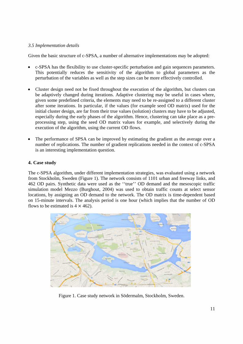
The c-SPSA algorithm, under different implementation strategies, was evaluated using a network from Stockholm, Sweden (Figure 1). The network consists of 1101 urban and freeway links, and 462 OD pairs. Synthetic data were used as the ‘‘true’’ OD demand and the mesoscopic traffic simulation model Mezzo (Burghout, 2004) was used to obtain traffic counts at select sensor locations, by assigning an OD demand to the network. The OD matrix is time-dependent based on 15-minute intervals. The analysis period is one hour (which implies that the number of OD flows to be estimated is 4 462).

Figure 1. Case study network in Södermalm, Stockholm, Sweden.

12

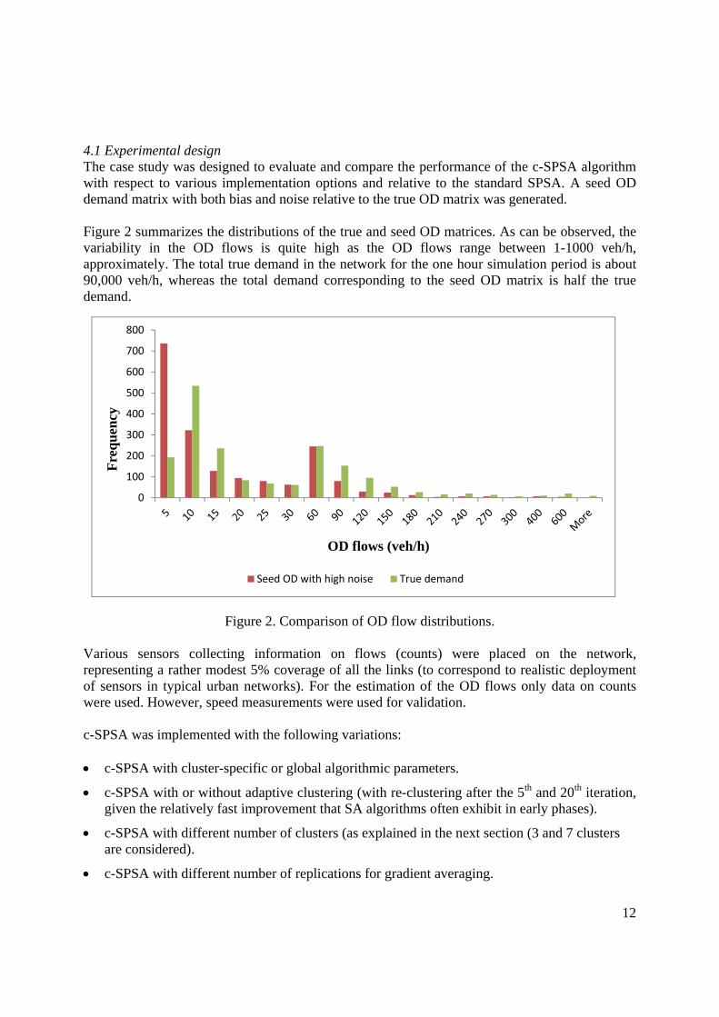
4.1 Experimental design The case study was designed to evaluate and compare the performance of the c-SPSA algorithm with respect to various implementation options and relative to the standard SPSA. A seed OD demand matrix with both bias and noise relative to the true OD matrix was generated. Figure 2 summarizes the distributions of the true and seed OD matrices. As can be observed, the variability in the OD flows is quite high as the OD flows range between 1-1000 veh/h, approximately. The total true demand in the network for the one hour simulation period is about 90,000 veh/h, whereas the total demand corresponding to the seed OD matrix is half the true demand.

Figure 2. Comparison of OD flow distributions.

Various sensors collecting information on flows (counts) were placed on the network, representing a rather modest 5% coverage of all the links (to correspond to realistic deployment of sensors in typical urban networks). For the estimation of the OD flows only data on counts were used. However, speed measurements were used for validation. c-SPSA was implemented with the following variations: c-SPSA with cluster-specific or global algorithmic parameters.

c-SPSA with or without adaptive clustering (with re-clustering after the 5th and 20th iteration, given the relatively fast improvement that SA algorithms often exhibit in early phases).

c-SPSA with different number of clusters (as explained in the next section (3 and 7 clusters are considered).

c-SPSA with different number of replications for gradient averaging.

0

100

200

300

400

500

600

700

800

Fre

qu

ency

OD flows (veh/h)

Seed OD with high noise True demand

13

Two aggregate measures of performance were used: the root-mean-square error (RMSE) and the mean absolute error (MAE) for OD flows, counts and speeds, relative to the true (observed) values:

∑ (18)

∑ | | (19)

Where, is the number of measurements, are estimated measurements, and are observed measurements. Theil’s inequality coefficient was also used to measure both relative error and bias (Toledo and Koutsopoulos, 2004):

∑

∑ ∑ (20)

assumes values between zero and one. 0 implies perfect fit between the estimated and

observed measurements, while 1 indicates the worst possible fit. Theil’s inequality coefficient is decomposed to three proportions of inequality: the bias , variance ( ) and covariance ( ) proportions:

∑ (21)

∑ (22)

∑ (23)

where , , and are the sample means and standard deviations of the observed and estimated measurements, respectively, and is the correlation coefficient between the two sets of measurements. The bias proportion is a measure of the systematic error of the identified solution and the variance proportion is an indication of how well the solution replicates the variability in the observed data. Values of less than 0.10 - 0.20 for these proportions indicate good performance. The covariance proportion measures the remaining error and should be close to one.

14

5. Results and discussion

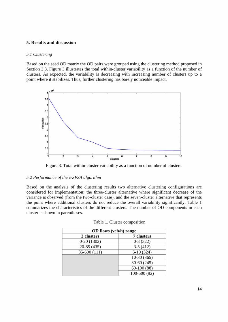
5.1 Clustering

Based on the seed OD matrix the OD pairs were grouped using the clustering method proposed in Section 3.3. Figure 3 illustrates the total within-cluster variability as a function of the number of clusters. As expected, the variability is decreasing with increasing number of clusters up to a point where it stabilizes. Thus, further clustering has barely noticeable impact.

Figure 3. Total within-cluster variability as a function of number of clusters.

5.2 Performance of the c-SPSA algorithm

Based on the analysis of the clustering results two alternative clustering configurations are considered for implementation: the three-cluster alternative where significant decrease of the variance is observed (from the two-cluster case), and the seven-cluster alternative that represents the point where additional clusters do not reduce the overall variability significantly. Table 1 summarizes the characteristics of the different clusters. The number of OD components in each cluster is shown in parentheses.

Table 1. Cluster composition

OD flows (veh/h) range3 clusters 7 clusters

0-20 (1302) 0-3 (322) 20-85 (435) 3-5 (412) 85-600 (111) 5-10 (324)

10-30 (365) 30-60 (245) 60-100 (88) 100-500 (92)

15

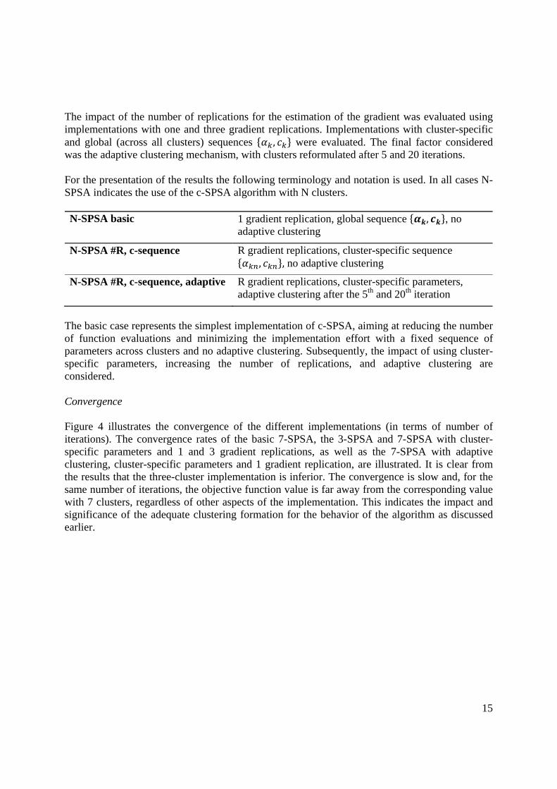
The impact of the number of replications for the estimation of the gradient was evaluated using implementations with one and three gradient replications. Implementations with cluster-specific and global (across all clusters) sequences , were evaluated. The final factor considered was the adaptive clustering mechanism, with clusters reformulated after 5 and 20 iterations. For the presentation of the results the following terminology and notation is used. In all cases N-SPSA indicates the use of the c-SPSA algorithm with N clusters. N-SPSA basic 1 gradient replication, global sequence , , no

adaptive clustering

N-SPSA #R, c-sequence R gradient replications, cluster-specific sequence , , no adaptive clustering

N-SPSA #R, c-sequence, adaptive R gradient replications, cluster-specific parameters, adaptive clustering after the 5th and 20th iteration

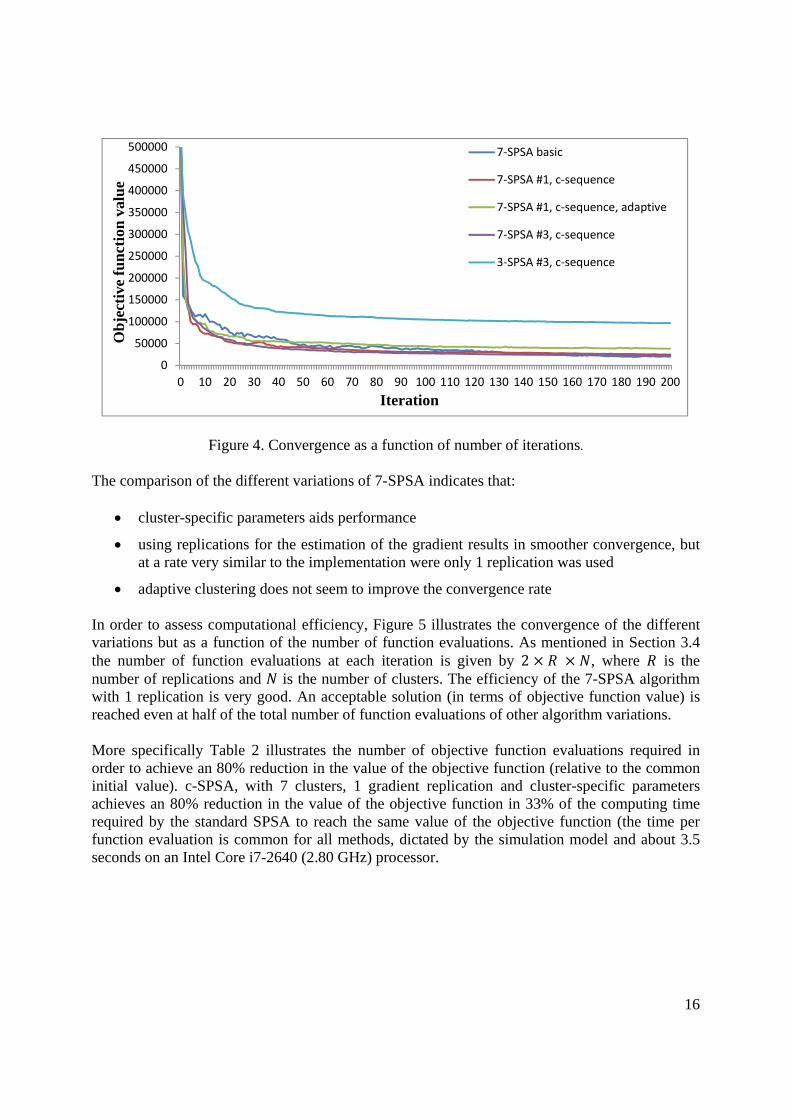
The basic case represents the simplest implementation of c-SPSA, aiming at reducing the number of function evaluations and minimizing the implementation effort with a fixed sequence of parameters across clusters and no adaptive clustering. Subsequently, the impact of using cluster-specific parameters, increasing the number of replications, and adaptive clustering are considered. Convergence Figure 4 illustrates the convergence of the different implementations (in terms of number of iterations). The convergence rates of the basic 7-SPSA, the 3-SPSA and 7-SPSA with cluster-specific parameters and 1 and 3 gradient replications, as well as the 7-SPSA with adaptive clustering, cluster-specific parameters and 1 gradient replication, are illustrated. It is clear from the results that the three-cluster implementation is inferior. The convergence is slow and, for the same number of iterations, the objective function value is far away from the corresponding value with 7 clusters, regardless of other aspects of the implementation. This indicates the impact and significance of the adequate clustering formation for the behavior of the algorithm as discussed earlier.

16

Figure 4. Convergence as a function of number of iterations.

The comparison of the different variations of 7-SPSA indicates that:

cluster-specific parameters aids performance

using replications for the estimation of the gradient results in smoother convergence, but at a rate very similar to the implementation were only 1 replication was used

adaptive clustering does not seem to improve the convergence rate In order to assess computational efficiency, Figure 5 illustrates the convergence of the different variations but as a function of the number of function evaluations. As mentioned in Section 3.4 the number of function evaluations at each iteration is given by 2 , where is the number of replications and is the number of clusters. The efficiency of the 7-SPSA algorithm with 1 replication is very good. An acceptable solution (in terms of objective function value) is reached even at half of the total number of function evaluations of other algorithm variations. More specifically Table 2 illustrates the number of objective function evaluations required in order to achieve an 80% reduction in the value of the objective function (relative to the common initial value). c-SPSA, with 7 clusters, 1 gradient replication and cluster-specific parameters achieves an 80% reduction in the value of the objective function in 33% of the computing time required by the standard SPSA to reach the same value of the objective function (the time per function evaluation is common for all methods, dictated by the simulation model and about 3.5 seconds on an Intel Core i7-2640 (2.80 GHz) processor.

0

50000

100000

150000

200000

250000

300000

350000

400000

450000

500000

0 10 20 30 40 50 60 70 80 90 100 110 120 130 140 150 160 170 180 190 200

Ob

ject

ive

fun

ctio

n v

alu

e

Iteration

7‐SPSA basic

7‐SPSA #1, c‐sequence

7‐SPSA #1, c‐sequence, adaptive

7‐SPSA #3, c‐sequence

3‐SPSA #3, c‐sequence

17

Figure 5. Convergence as a function of number of function evaluations.

Table 2 Number of function evaluations

Quality of solution

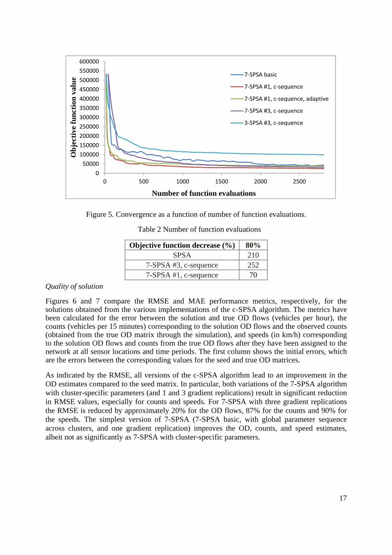
Figures 6 and 7 compare the RMSE and MAE performance metrics, respectively, for the solutions obtained from the various implementations of the c-SPSA algorithm. The metrics have been calculated for the error between the solution and true OD flows (vehicles per hour), the counts (vehicles per 15 minutes) corresponding to the solution OD flows and the observed counts (obtained from the true OD matrix through the simulation), and speeds (in km/h) corresponding to the solution OD flows and counts from the true OD flows after they have been assigned to the network at all sensor locations and time periods. The first column shows the initial errors, which are the errors between the corresponding values for the seed and true OD matrices.

As indicated by the RMSE, all versions of the c-SPSA algorithm lead to an improvement in the OD estimates compared to the seed matrix. In particular, both variations of the 7-SPSA algorithm with cluster-specific parameters (and 1 and 3 gradient replications) result in significant reduction in RMSE values, especially for counts and speeds. For 7-SPSA with three gradient replications the RMSE is reduced by approximately 20% for the OD flows, 87% for the counts and 90% for the speeds. The simplest version of 7-SPSA (7-SPSA basic, with global parameter sequence across clusters, and one gradient replication) improves the OD, counts, and speed estimates, albeit not as significantly as 7-SPSA with cluster-specific parameters.

Objective function decrease (%) 80% SPSA 210

7-SPSA #3, c-sequence 252 7-SPSA #1, c-sequence 70

0

50000

100000

150000

200000

250000

300000

350000

400000

450000

500000

550000

600000

0 500 1000 1500 2000 2500

Ob

ject

ive

func

tion

val

ue

Number of function evaluations

7‐SPSA basic

7‐SPSA #1, c‐sequence

7‐SPSA #1, c‐sequence, adaptive

7‐SPSA #3, c‐sequence

3‐SPSA #3, c‐sequence

18

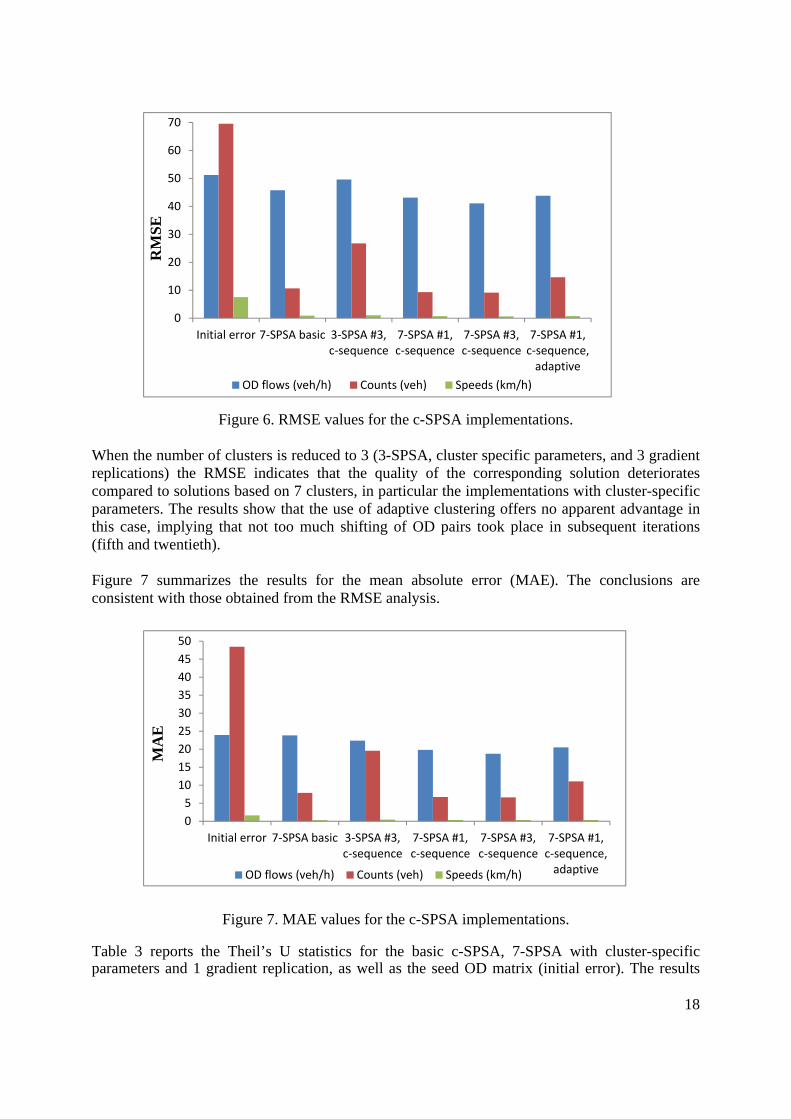
Figure 6. RMSE values for the c-SPSA implementations. When the number of clusters is reduced to 3 (3-SPSA, cluster specific parameters, and 3 gradient replications) the RMSE indicates that the quality of the corresponding solution deteriorates compared to solutions based on 7 clusters, in particular the implementations with cluster-specific parameters. The results show that the use of adaptive clustering offers no apparent advantage in this case, implying that not too much shifting of OD pairs took place in subsequent iterations (fifth and twentieth). Figure 7 summarizes the results for the mean absolute error (MAE). The conclusions are consistent with those obtained from the RMSE analysis.

Figure 7. MAE values for the c-SPSA implementations.

Table 3 reports the Theil’s U statistics for the basic c-SPSA, 7-SPSA with cluster-specific parameters and 1 gradient replication, as well as the seed OD matrix (initial error). The results

0

5

10

15

20

25

30

35

40

45

50

Initial error 7‐SPSA basic 3‐SPSA #3,c‐sequence

7‐SPSA #1,c‐sequence

7‐SPSA #3,c‐sequence

7‐SPSA #1,c‐sequence,adaptive

MA

E

OD flows (veh/h) Counts (veh) Speeds (km/h)

0

10

20

30

40

50

60

70

Initial error 7‐SPSA basic 3‐SPSA #3,c‐sequence

7‐SPSA #1,c‐sequence

7‐SPSA #3,c‐sequence

7‐SPSA #1,c‐sequence,adaptive

RM

SE

OD flows (veh/h) Counts (veh) Speeds (km/h)

19

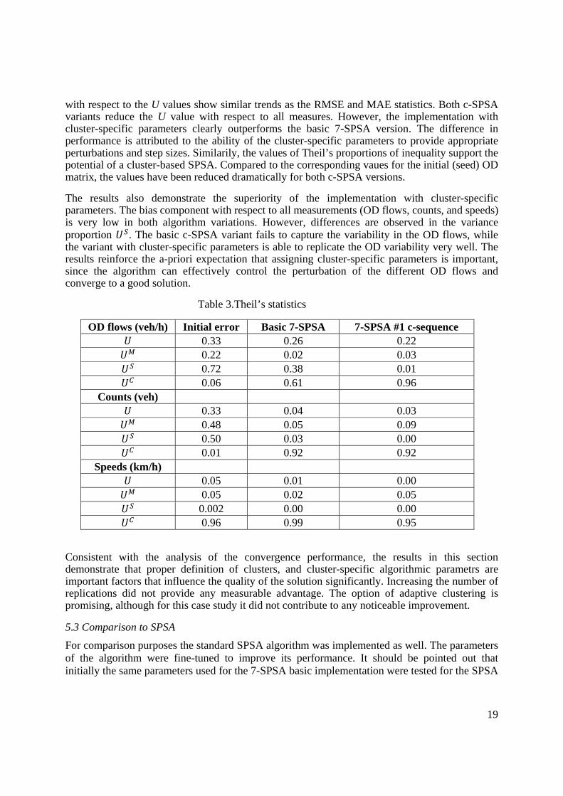
with respect to the U values show similar trends as the RMSE and MAE statistics. Both c-SPSA variants reduce the U value with respect to all measures. However, the implementation with cluster-specific parameters clearly outperforms the basic 7-SPSA version. The difference in performance is attributed to the ability of the cluster-specific parameters to provide appropriate perturbations and step sizes. Similarily, the values of Theil’s proportions of inequality support the potential of a cluster-based SPSA. Compared to the corresponding vaues for the initial (seed) OD matrix, the values have been reduced dramatically for both c-SPSA versions.

The results also demonstrate the superiority of the implementation with cluster-specific parameters. The bias component with respect to all measurements (OD flows, counts, and speeds) is very low in both algorithm variations. However, differences are observed in the variance proportion . The basic c-SPSA variant fails to capture the variability in the OD flows, while the variant with cluster-specific parameters is able to replicate the OD variability very well. The results reinforce the a-priori expectation that assigning cluster-specific parameters is important, since the algorithm can effectively control the perturbation of the different OD flows and converge to a good solution.

Table 3.Theil’s statistics

OD flows (veh/h) Initial error Basic 7-SPSA 7-SPSA #1 c-sequence 0.33 0.26 0.22 0.22 0.02 0.03 0.72 0.38 0.01 0.06 0.61 0.96

Counts (veh) 0.33 0.04 0.03 0.48 0.05 0.09 0.50 0.03 0.00 0.01 0.92 0.92

Speeds (km/h) 0.05 0.01 0.00 0.05 0.02 0.05 0.002 0.00 0.00 0.96 0.99 0.95

Consistent with the analysis of the convergence performance, the results in this section demonstrate that proper definition of clusters, and cluster-specific algorithmic parametrs are important factors that influence the quality of the solution significantly. Increasing the number of replications did not provide any measurable advantage. The option of adaptive clustering is promising, although for this case study it did not contribute to any noticeable improvement.

5.3 Comparison to SPSA

For comparison purposes the standard SPSA algorithm was implemented as well. The parameters of the algorithm were fine-tuned to improve its performance. It should be pointed out that initially the same parameters used for the 7-SPSA basic implementation were tested for the SPSA

20

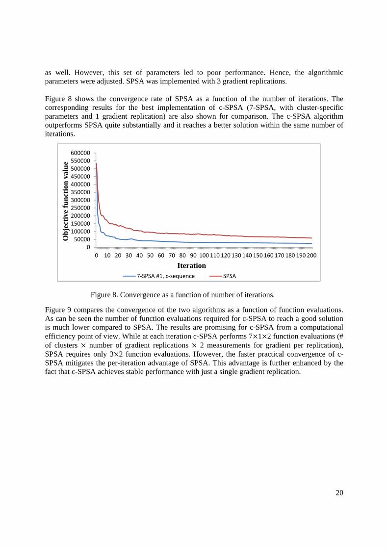
as well. However, this set of parameters led to poor performance. Hence, the algorithmic parameters were adjusted. SPSA was implemented with 3 gradient replications. Figure 8 shows the convergence rate of SPSA as a function of the number of iterations. The corresponding results for the best implementation of c-SPSA (7-SPSA, with cluster-specific parameters and 1 gradient replication) are also shown for comparison. The c-SPSA algorithm outperforms SPSA quite substantially and it reaches a better solution within the same number of iterations.

Figure 8. Convergence as a function of number of iterations.

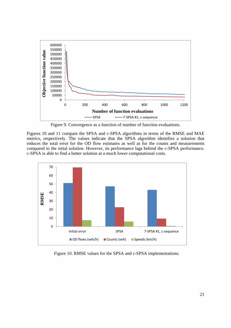
Figure 9 compares the convergence of the two algorithms as a function of function evaluations. As can be seen the number of function evaluations required for c-SPSA to reach a good solution is much lower compared to SPSA. The results are promising for c-SPSA from a computational efficiency point of view. While at each iteration c-SPSA performs 7 1 2 function evaluations (# of clusters number of gradient replications 2 measurements for gradient per replication), SPSA requires only 3 2 function evaluations. However, the faster practical convergence of c-SPSA mitigates the per-iteration advantage of SPSA. This advantage is further enhanced by the fact that c-SPSA achieves stable performance with just a single gradient replication.

050000

100000150000200000250000300000350000400000450000500000550000600000

0 10 20 30 40 50 60 70 80 90 100 110 120 130 140 150 160 170 180 190 200

Ob

ject

ive

fun

ctio

n v

alu

e

Iteration7‐SPSA #1, c‐sequence SPSA

21

Figure 9. Convergence as a function of number of function evaluations.

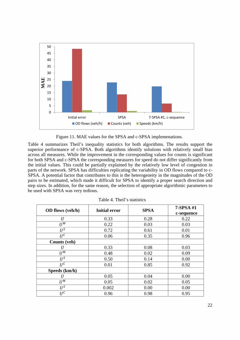
Figures 10 and 11 compare the SPSA and c-SPSA algorithms in terms of the RMSE and MAE metrics, respectively. The values indicate that the SPSA algorithm identifies a solution that reduces the total error for the OD flow estimates as well as for the counts and measurements compared to the intial solution. However, its performance lags behind the c-SPSA performance. c-SPSA is able to find a better solution at a much lower computational costs.

Figure 10. RMSE values for the SPSA and c-SPSA implementations.

0

10

20

30

40

50

60

70

Initial error SPSA 7‐SPSA #1, c‐sequence

RM

SE

OD flows (veh/h) Counts (veh) Speeds (km/h)

050000100000150000200000250000300000350000400000450000500000550000600000

0 200 400 600 800 1000 1200

Ob

ject

ive

fun

ctio

n v

alu

e

Number of function evaluationsSPSA 7‐SPSA #1, c‐sequence

22

Figure 11. MAE values for the SPSA and c-SPSA implemenations.

Table 4 summarizes Theil’s inequality statistics for both algorithms. The results support the superior performance of c-SPSA. Both algorithms identify solutions with relatively small bias across all measures. While the improvement in the corresponding values for counts is significant for both SPSA and c-SPSA the corresponding measures for speed do not differ significantly from the initial values. This could be partially explained by the relatively low level of congestion in parts of the network. SPSA has difficulties replicating the variability in OD flows compared to c-SPSA. A potential factor that contributes to this is the heterogeneity in the magnitudes of the OD pairs to be estimated, which made it difficult for SPSA to identify a proper search direction and step sizes. In addition, for the same reason, the selection of appropriate algorithmic parameters to be used with SPSA was very tedious.

Table 4. Theil’s statistics

OD flows (veh/h) Initial error SPSA 7-SPSA #1 c-sequence

0.33 0.28 0.22 0.22 0.03 0.03 0.72 0.61 0.01 0.06 0.35 0.96

Counts (veh) 0.33 0.08 0.03 0.48 0.02 0.09 0.50 0.14 0.00 0.01 0.85 0.92

Speeds (km/h) 0.05 0.04 0.00 0.05 0.02 0.05 0.002 0.00 0.00 0.96 0.98 0.95

0

5

10

15

20

25

30

35

40

45

50

Initial error SPSA 7‐SPSA #1, c‐sequence

MA

E

OD flows (veh/h) Counts (veh) Speeds (km/h)

23

6 Conclusion A modification of the stochastic approximation algorithm SPSA, referred to as cluster-based SPSA (c-SPSA), is proposed motivated by the need to solve dynamic OD estimation problems with data from various sources. Such general formulations of the OD estimation problem rely on simulation and have been solved in the past using the SPSA algorithm. SPSA has a number of disadvantages related to stability and sensitivity to a set of parameters that govern the perturbation and step size. The new algorithm uses a segmentation of the unknown vector into “homogeneous” clusters. The gradient is then estimated by simultaneously perturbing the elements of the unknown vector that belong to the same cluster, while all other variables remain fixed to their current value. An approach for cluster design is also proposed based on the k-means method. The paper establishes the theoretical properties of the algorithm with an upper bound for the bias of the estimated gradient and shows that it is lower than the corresponding bound of SPSA. Because of the greater uniformity within each cluster, it is also expected that the algorithm will be more robust, less sensitive to the choice of algorithmic parameters, and with improved practical convergence. Different implementations of c-SPSA (number of clusters, number of replications, cluster-specific parameters, and adaptive clustering) were evaluated through a case study using a network from Stockholm, Sweden and a synthetic OD matrix. The number of clusters and cluster-specific parameters were the most important implementation factors of c-SPSA and provided the greatest improvement. The performance of c-SPSA was also compared to the standard SPSA algorithm. The results support the a-priori expectations. c-SPSA outperformed SPSA not only in terms of stability and quality of solution, but also in computational efficiency. c-SPSA was able to identify superior solutions with much lower number of function evaluations. A factor that contributed to the computational efficiency, in addition to better practical convergence performance, was the fact that c-SPSA had good performance even when only one replication was used for gradient estimation. The effort required for fine-tuning of the algorithmic parameters was also less cumbersome compared to SPSA, especially for implementations of c-SPSA with cluster-specific parameters. The within-cluster uniformity makes their determination easier. Acknowledgments The authors would like to acknowledge the financial support from the Swedish National Transport Administration and Trafik Stockholm for data and other information related to the network. The authors would like to thank the reviewers for their constructive comments and suggestions. References

Andradóttir, S., 1996. A Scaled Stochastic Approximation Algorithm. Management Science 42 (4), 475–98.

24

Azavidvar, F., 1992. A tutorial on simulation optimization. 24th Winter Simulation Conference, Arlington, VA, USA.

Balakrishna, R., 2006. Off-line Calibration of dynamic Traffic Assignment Models. Ph.D thesis. Massachusetts Institute of Technology, Cambridge.

Balakrishna, R., Ben-Akiva, M., Koutsopoulos, H.N., 2007. Off-line calibration of dynamic traffic assignment: Simultaneous demand-supply estimation. Trans. Res. Rec., 2003, 50-58.

Balakrishna, R., Ben-Akiva, M. and Koutsopoulos, H.N., 2008 Time-Dependent Origin-Destination Estimation Without Assignment Matrices. Chapter 12, in Traffic Simulation E. Chung and A-G- Dumont, editors, EPFL Press, pp 201-213.

Balakrishna, R., and Koutsopoulos, H.N., 2008. Incorporating Within-Day Transitions in Simultaneous Estimation of Dynamic Origin-Destination Flows Without Assignment Matrices. Trans. Res. Rec., 2085, 31-38, doi: 10.3141/2085-04.

Blum, J.R., 1954. Multidimensional Stochastic Approximation Methods. Annals of Mathematical Statistics 25, pp. 737-744.

Broadie, Cicek, M.D., Zeevi, A., 2014. Multidimensional stochastic approximation: adaptive algorithms and applications. ACM Trans. Model Comput. Simul. 24 (1).

Burghout, W., 2004. Hybrid microscopic-mesoscopic traffic simulation. Ph.D. thesis. Dept. Infrastructure, Div. Transp. Logistics, Royal Inst. Technol., Stockholm, Sweden.

Cantelmo, G., Viti, F., Tampere, C., M.J., Cipriani, E., Nigro, M. (2014). A two-step approach for the correction of the seed matrix in the dynamic demand estimation. Proceeding of the 93rd Annual Meeting in Transportation Research Board, TRB 2014.

Cascetta E., and Postorino, M. N., 2001. Fixed Point Approaches to the Estimation of O/D Matrices Using Traffic Counts on Congested Networks. Transportation Science, 35, (2), 134-137.

Cipriani, E., Florian, M., Mahut, M., Nigro, M., 2011. A gradient approximation approach for adjusting temporal origin-destination matrices. Transp. Research Part C 19, 270-282.

Cipriani, E., Nigro, M., Fusco, G., Colombaroni, C., 2014. Effectiveness of link and path information on simultaneous adjustment of dynamic O-D demand matrix. Eur. Transp. Res. Rev. 6 (2), 139-148.

Cipriani, E., Gemma, A., Nigro, M., 2013. A bi-level gradient approximation method for dynamic traffic demand estimation: sensitivity analysis and adaptive approach. Intelligent Transportation Systems Conference, The Hague, October 6-9, pp. 2100-2105.

Frederix, R., Viti, F., Corthout, F., Tampere, C., 2011. New Gradient Approximation Method for Dynamic Origin-Destination Matrix Estimation on Congested Networks. Trans. Res. Rec. 2263, 19-25.

25

Kiefer, J., Wolfowitz, J., 1952. Stochastic estimation of a regression function, Annals of Mathematical Statistics 23, 462-466.

Mishalani R. G., Koutsopoulos H. N, 2002. Modeling the spatial behavior of infrastructure condition. Transp. Res. Part B 36, 171-194.

Robbins, H., Monro, S., 1951. A stochastic approximation method, Annals of Mathematical Statistics 22, 400-407.

Spall, J.C., 1992. Multivariate stochastic approximation using a simultaneous perturbation gradient approximation. IEEE Trans. Automat. Control 37 (3), 332-341.

Spall, J.C., 1994. Developments in stochastic optimization algorithms with gradient approximations based on function measurements. 26th Winter Simulation Conference, 207–14.

Spall, J.C., 1998. Implementation of the simultaneous perturbation algorithm for stochastic optimization. IEEE Trans. Aerosp. Electron. Syst. 34 (3), 817-823.

Spall, J.C., 1999. Stochastic optimization, stochastic approximation and simulated annealing. Wiley Encyclopedia of electrical and Electronics Engineering 20, 529-542.

Spall, J. C., 2000. Adaptive stochastic approximation by the simultaneous perturbation method. IEEE Trans. Automat. Control 45 (10), 1839-1853.

Spall, J.C., 2003. Introduction to stochastic search optimization: Estimation, simulation and control, Wiley, Hoboken, NJ.

Spiess, H., 1990. A gradient approach for the O–D matrix adjustment problem. Transp. Res. Centre, Montreal Univ., Quebec. Canada, Publication 693.

Toledo, T., Kolechkina, T., 2013. Estimation of dynamic origin-destination matrices using linear assignment matrix approximations. IEEE Trans. Intell. Trans. Syst. 14 (2), 618-626.

Toledo T., and Koutsopoulos, H. N., 2004. Statistical Validation of Traffic Simulation Models. Transp. Res. Rec., 1876, 142-150, doi: 10.3141/1876-15.

Vaze, V., Antoniou, C., Wen, Y., Ben-Akiva, M., 2009. Calibration of dynamic traffic assignment models with point-to-point traffic surveillance, Transp. Res. Rec., 2090, 1-9.

Xu, Z., Wu, X., 2013. A New Hybrid Stochastic Approximation Algorithm. Optim. Lett. 7 (3), 593–606.