arX

iv:0

901.

3245

v1 [

mat

h.ST

] 2

1 Ja

n 20

09

The Annals of Statistics

2008, Vol. 36, No. 6, 2791–2817DOI: 10.1214/08-AOS618c© Institute of Mathematical Statistics, 2008

FINITE SAMPLE APPROXIMATION RESULTS

FOR PRINCIPAL COMPONENT ANALYSIS:

A MATRIX PERTURBATION APPROACH1

By Boaz Nadler

Weizmann Institute of Science

Principal component analysis (PCA) is a standard tool for di-mensional reduction of a set of n observations (samples), each withp variables. In this paper, using a matrix perturbation approach, westudy the nonasymptotic relation between the eigenvalues and eigen-vectors of PCA computed on a finite sample of size n, and those ofthe limiting population PCA as n →∞. As in machine learning, wepresent a finite sample theorem which holds with high probabilityfor the closeness between the leading eigenvalue and eigenvector ofsample PCA and population PCA under a spiked covariance model.In addition, we also consider the relation between finite sample PCAand the asymptotic results in the joint limit p,n →∞, with p/n = c.We present a matrix perturbation view of the “phase transition phe-nomenon,” and a simple linear-algebra based derivation of the eigen-value and eigenvector overlap in this asymptotic limit. Moreover, ouranalysis also applies for finite p,n where we show that although thereis no sharp phase transition as in the infinite case, either as a func-tion of noise level or as a function of sample size n, the eigenvector ofsample PCA may exhibit a sharp “loss of tracking,” suddenly losingits relation to the (true) eigenvector of the population PCA matrix.This occurs due to a crossover between the eigenvalue due to the sig-nal and the largest eigenvalue due to noise, whose eigenvector pointsin a random direction.

1. Introduction. Principal component analysis (PCA) is a standard toolfor dimensionality reduction, applied in regression, classification and manyother data analysis tasks in a variety of scientific fields [17, 20]. PCA findsorthonormal directions with maximal variance of the data and allows its

Received February 2007; revised February 2008.1Supported by the Lord Sieff of Brimpton memorial fund and by the Hana and Julius

Rosen fund.AMS 2000 subject classifications. Primary 62H25, 62E17; secondary 15A42.Key words and phrases. Principal component analysis, spiked covariance model, ran-

dom matrix theory, matrix perturbation, phase transition.

This is an electronic reprint of the original article published by theInstitute of Mathematical Statistics in The Annals of Statistics,2008, Vol. 36, No. 6, 2791–2817. This reprint differs from the original inpagination and typographic detail.

1

2 B. NADLER

low-dimensional representation by linear projections onto these directions.This dimensionality reduction is a typical preprocessing step in many clas-sification and regression problems.

Assuming the given data is a finite and random sample from a (generallyunknown) distribution, an interesting theoretical and practical question isthe relation between the sample PCA results computed from finite data andthose of the underlying population model. In this paper we consider a spikedcovariance model for which the underlying data is low-dimensional but eachsample is corrupted by additive Gaussian noise, and analyze the followingquestion: how close are the directions and eigenvalues computed by samplePCA to the limiting (and generally unknown) directions and eigenvalues ofthe population model and how do these quantities depend on the number ofsamples n, the dimensionality p and the noise level σ.

Many works have studied the convergence of eigenvalues and eigenvec-tors of sample PCA to those of population PCA under various settings. Ingeneral, the different results regarding convergence can be divided into twomain types: (i) asymptotic results of classical statistics, where p is fixed andn →∞, starting with the classical works of Girshick [12], Lawley [23] andAnderson [1], who assumed multivariate Gaussian distributions, up to morerecent work which relaxed some of these assumptions; see [2, 17] and ref-erences therein; (ii) modern “large p, large n” statistical results, where thejoint limit p,n→∞ is considered while the ratio p/n = c is kept fixed. In thestatistical physics literature we mention Hoyle and Rattray [14], Reimann,Van den Broeck and Bex [32], Watkin and Nadal [37], Biehl and Mietzner [5]and references therein, whereas in the statistics community see the recentworks by Johnstone [18], Baik and Silverstein [4], Debashis [31], Onatski[29] and many references therein for older works. However, it seems thatthe most relevant case, that of explicit approximation bounds between theeigenvalues and eigenvectors computed in a finite setting (p,n finite) andthose of the infinite setting (p fixed, n = ∞), as well as estimates of the dis-tributions of these quantities (again for finite and fixed p,n), are not coveredby these approaches.

In the present work we address this problem using a combination of ma-trix perturbation theory and concentration of measure bounds on the normof noisy Wishart matrices. This paper contains two main contributions. Firstwe present probabilistic approximation results regarding the difference be-tween the leading eigenvalue and eigenvector of sample PCA and populationPCA for fixed p and n, under a spiked covariance model with a single com-ponent. The second contribution of this paper is a matrix perturbation viewof the phase transition for the leading eigenvalue and eigenvector, whenboth p,n are large. We present a simple linear-algebra based proof of theasymptotics of the leading eigenvalue and eigenvector in the limit p,n→∞.Second, we present an interesting connection between this asymptotic value

FINITE SAMPLE APPROXIMATION RESULTS 3

and a classical result by Lawley. This observation leads to two additionalpropositions, one regarding the limiting eigenvalues for a more general spikedcovariance model, and one regarding the spectral norm of a noisy Wishartmatrix with nonidentity diagonal covariance matrix. These results may beuseful for inference on the number of significant components under moregeneral settings of heteroscedastic correlated noise. Finally, for finite p,n weshow that while there is no deterministic phase transition at a specific fixedvalue of p/n, either as a function of noise level or as a function of samplesize, the eigenvector of sample PCA may exhibit a sharp “loss of tracking,”suddenly losing its relation to the (true) eigenvector of the population PCAmatrix. This occurs due to a crossover between the eigenvalue due to thesignal and the largest eigenvalue due to noise, whose eigenvector points in arandom direction.

Matrix perturbation theory, including eigenvalue and eigenvector pertur-bation bounds, as well as the structure of eigenvalues and eigenvectors ofarrowhead matrices, play a key role in the analysis of both finite samplePCA and the asymptotic limit p,n →∞. Perturbation theory and concen-tration of measure results on the norm of noisy Wishart matrices are keyingredients in the analysis of the finite sample case, and also provide novelinsight into the origins of the phase transition in the joint limit p,n →∞.In the statistics literature, matrix perturbation theory is typically used tobound remainder terms in asymptotic limits. In the context of PCA, forexample, in [10] Eaton and Tyler used a perturbation bound by Wielandt topresent a simple derivation of asymptotic results as n →∞ for eigenvalues ofrandom symmetric matrices, but did not consider the nonasymptotic case.In [35], Stewart introduced a general framework of stochastic perturbationtheory to analyze the effects of random perturbations on the eigenvalues offinite matrices, whereas perturbation bounds for the singular value decom-position were considered in [36]. Within the context of the spiked covariancemodel, matrix perturbation theory was used in [4, 19, 31], though theseworks considered mainly the asymptotic limit p,n→∞.

From a practical point of view, our results show that when p,n are large,and specifically when p ≫ n, the true signal directions may be drownedby noise since for finite p ≫ n, eigenvector reconstruction errors behaveas σ

√

p/n, as also predicted by the asymptotic analysis of Johnstone andLu [19]. A similar phenomenon also occurs in linear discriminant analy-sis [6], and for various multivariate regression algorithms such as partialleast squares and classical least squares [26]. All these works emphasize theimportance of regularization, feature selection or low-dimensional represen-tation prior to learning, and hint that global methods may not be optimalfor dimensional reduction or as a preprocessing step prior to regression andclassification of high-dimensional noisy data, specifically if there is a prioriknowledge regarding its sparsity or smoothness. The results and approach

4 B. NADLER

presented in this paper can also be used to develop methods to determinethe number of components in a linear mixture (spiked covariance) model[22].

The paper is organized as follows. In Section 2 we present the spikedcovariance model and our main results. The results for finite p,n are provenin Sections 3 and 4. A matrix perturbation view of the phase transitionphenomenon in the joint limit as p,n→∞, as well an analysis of the spikedcovariance model under more general models of noise and some finite sampleexamples appear in Section 5.

2. Model, assumptions and main results.

2.1. Notation. Univariate random variables are denoted by lowercase let-ters, as in u, their realizations are denoted by uν and their expectation byE{u}. Column vectors are denoted by boldface lowercase letters, as in x,their transpose is x

T , their jth component is xj the dot product betweentwo vectors is 〈x,z〉, and the Euclidean (L2) norm of x is ‖x‖. Matrices aredenoted by uppercase letters, as in A. The identity matrix of order p is Ip,and the spectral norm of a matrix A is ‖A‖.

2.2. The spiked covariance model. We consider a spiked covariance modelwhere each data sample x has the form

x =k∑

i=1

uivi + σξ,(2.1)

where {ui}ki=1 are random variables, typically called components or latent

variables, {vi}ki=1 ⊂ R

p are the corresponding fixed (and typically unknown)response vectors, ξ is a multivariate Gaussian noise vector with identity co-variance matrix and σ is the level of noise. Equation (2.1) is an error-in-variables linear mixture model, commonly assumed in many different prob-lems and applications, including independent component analysis (ICA) [15],signal processing, and in the analysis of spectroscopic data, where it is knownas Beer’s law [25, 27].

We denote by Σ the p× p population covariance matrix corresponding tothe observations x,

Σ = E{xxT },(2.2)

and by Sn the sample covariance matrix corresponding to the n i.i.d. obser-vations {xν}n

ν=1,

Sn =1

n

n∑

ν=1

xν(xν)T .(2.3)

FINITE SAMPLE APPROXIMATION RESULTS 5

Assuming that all k vectors vj are orthogonal and that all k random vari-ables in (2.1) are uncorrelated with zero mean, unit variance and finitefourth moment, it follows that the largest k eigenvalue/eigenvector pairs ofΣ are given by {(‖vj‖2 + σ2,vj)}k

j=1. PCA approximates the eigenvaluesand eigenvectors of the unknown Σ by those of Sn. In particular, the topeigenvectors of Sn correspond to orthogonal directions of maximal varianceof the observed data. The question at hand, then, is how close are the largesteigenvalues and corresponding eigenvectors of Sn to those of Σ.

In this paper we present a matrix perturbation view of this problem.For simplicity we consider the case of a single component (k = 1). A simi-lar though more complicated analysis can be carried out for the case of kcomponents. We thus consider n samples from the model

x = uv + σξ,(2.4)

where we assume that the random variable u has zero mean, unit varianceand finite fourth moment. Without loss of generality, we further assume thatthe vector v is in the direction of e1 = (1,0, . . . ,0), for example, v = ‖v‖e1.Finally, since u has zero mean, we neglect in our analysis the initial meancentering step typically done in PCA.

The population covariance matrix corresponding to this one-componentmodel is given by

Σ =

‖v‖2 0 · · · 00 0 · · · 0...

. . ....

0 0 · · · 0

+ σ2Ip.(2.5)

Its largest eigenvalue is ‖v‖2 + σ2 with corresponding eigenvector e1, andall other eigenvalues equal σ2.

2.3. Results for finite p,n. To study the relationship between the samplecovariance matrix and the population matrix we introduce the followingquantities. Let {uν}n

ν=1 and {ξν}nν=1 denote the realizations of the r.v. u

and of the noise vector ξ in the given dataset {xν}nν=1. Let vPCA denote the

eigenvector of the sample covariance matrix Sn with largest eigenvalue λPCA.Our goal is to find the relation between the finite sample values (λPCA,vPCA)and the limiting values (‖v‖2 + σ2,e1). Since with an exponentially smallbut nonzero probability λPCA may be arbitrarily small and 〈vPCA,e1〉 maybe arbitrarily close to zero, we construct highly probable bounds on thesequantities, for example, bounds that hold with probability at least 1 − ε,where hopefully ε ≪ 1. This is common practice both in machine learningand in concentration of measure results.

6 B. NADLER

As we shall see below, the following quantities come into play in theanalysis:

s2u =

1

n

n∑

ν=1

(uν)2, κ = ‖v‖su,(2.6)

ρj =1

nsu

n∑

ν=1

uνξνj , βij =

1

n

n∑

ν=1

ξνi ξν

j .(2.7)

Loosely speaking, su is the second moment of the variable u, which is closeto unity for large n, κ is the “signal strength” for the given dataset, therandom variables ρj capture the signal–noise interactions, and βij are purenoise terms.

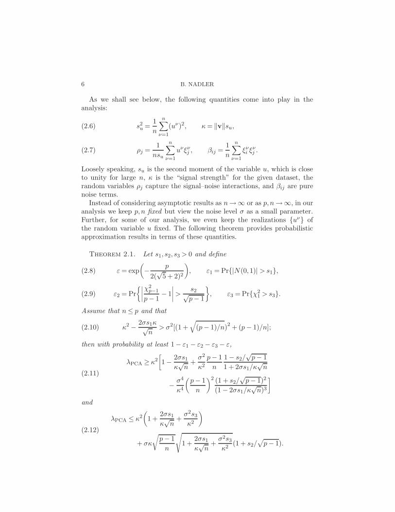
Instead of considering asymptotic results as n→∞ or as p,n →∞, in ouranalysis we keep p,n fixed but view the noise level σ as a small parameter.Further, for some of our analysis, we even keep the realizations {uν} ofthe random variable u fixed. The following theorem provides probabilisticapproximation results in terms of these quantities.

Theorem 2.1. Let s1, s2, s3 > 0 and define

ε = exp

(

− p

2(√

5 + 2)2

)

, ε1 = Pr{|N(0,1)| > s1},(2.8)

ε2 = Pr

{∣

∣

∣

∣

χ2p−1

p− 1− 1

∣

∣

∣

∣

>s2√p− 1

}

, ε3 = Pr{χ21 > s3}.(2.9)

Assume that n ≤ p and that

κ2 − 2σs1κ√n

> σ2[(1 +√

(p− 1)/n)2 + (p− 1)/n];(2.10)

then with probability at least 1− ε1 − ε2 − ε3 − ε,

λPCA ≥ κ2[

1− 2σs1

κ√

n+

σ2

κ2

p− 1

n

1− s2/√

p− 1

1 + 2σs1/κ√

n(2.11)

− σ4

κ4

(

p− 1

n

)2 (1 + s2/√

p− 1)2

(1− 2σs1/κ√

n)3

]

and

λPCA ≤ κ2(

1 +2σs1

κ√

n+

σ2s3

κ2

)

(2.12)

+ σκ

√

p− 1

n

√

1 +2σs1

κ√

n+

σ2s3

κ2(1 + s2/

√

p− 1).

FINITE SAMPLE APPROXIMATION RESULTS 7

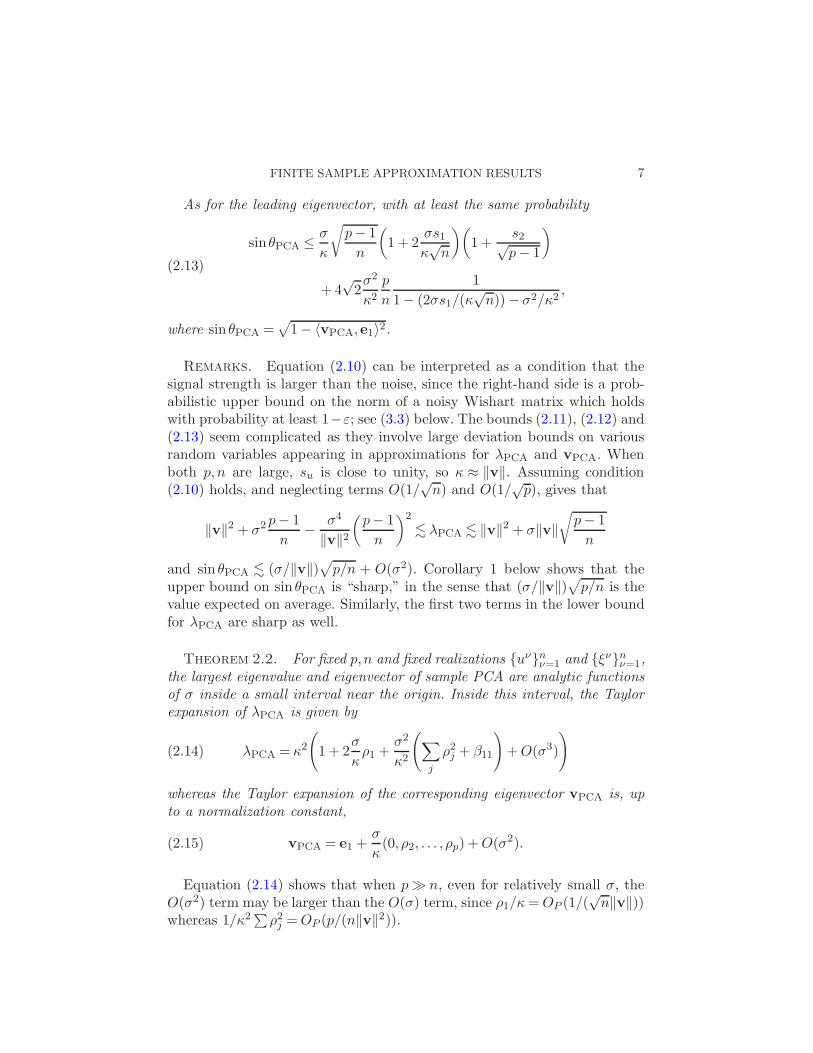
As for the leading eigenvector, with at least the same probability

sinθPCA ≤ σ

κ

√

p− 1

n

(

1 + 2σs1

κ√

n

)(

1 +s2√p− 1

)

(2.13)

+ 4√

2σ2

κ2

p

n

1

1− (2σs1/(κ√

n))− σ2/κ2,

where sinθPCA =√

1− 〈vPCA,e1〉2.

Remarks. Equation (2.10) can be interpreted as a condition that thesignal strength is larger than the noise, since the right-hand side is a prob-abilistic upper bound on the norm of a noisy Wishart matrix which holdswith probability at least 1−ε; see (3.3) below. The bounds (2.11), (2.12) and(2.13) seem complicated as they involve large deviation bounds on variousrandom variables appearing in approximations for λPCA and vPCA. Whenboth p,n are large, su is close to unity, so κ ≈ ‖v‖. Assuming condition(2.10) holds, and neglecting terms O(1/

√n) and O(1/

√p), gives that

‖v‖2 + σ2 p− 1

n− σ4

‖v‖2

(

p− 1

n

)2

. λPCA . ‖v‖2 + σ‖v‖√

p− 1

n

and sin θPCA . (σ/‖v‖)√

p/n + O(σ2). Corollary 1 below shows that theupper bound on sin θPCA is “sharp,” in the sense that (σ/‖v‖)

√

p/n is thevalue expected on average. Similarly, the first two terms in the lower boundfor λPCA are sharp as well.

Theorem 2.2. For fixed p,n and fixed realizations {uν}nν=1 and {ξν}n

ν=1,the largest eigenvalue and eigenvector of sample PCA are analytic functionsof σ inside a small interval near the origin. Inside this interval, the Taylorexpansion of λPCA is given by

λPCA = κ2

(

1 + 2σ

κρ1 +

σ2

κ2

(

∑

j

ρ2j + β11

)

+ O(σ3)

)

(2.14)

whereas the Taylor expansion of the corresponding eigenvector vPCA is, upto a normalization constant,

vPCA = e1 +σ

κ(0, ρ2, . . . , ρp) + O(σ2).(2.15)

Equation (2.14) shows that when p ≫ n, even for relatively small σ, theO(σ2) term may be larger than the O(σ) term, since ρ1/κ = OP (1/(

√n‖v‖))

whereas 1/κ2∑ρ2j = OP (p/(n‖v‖2)).

8 B. NADLER

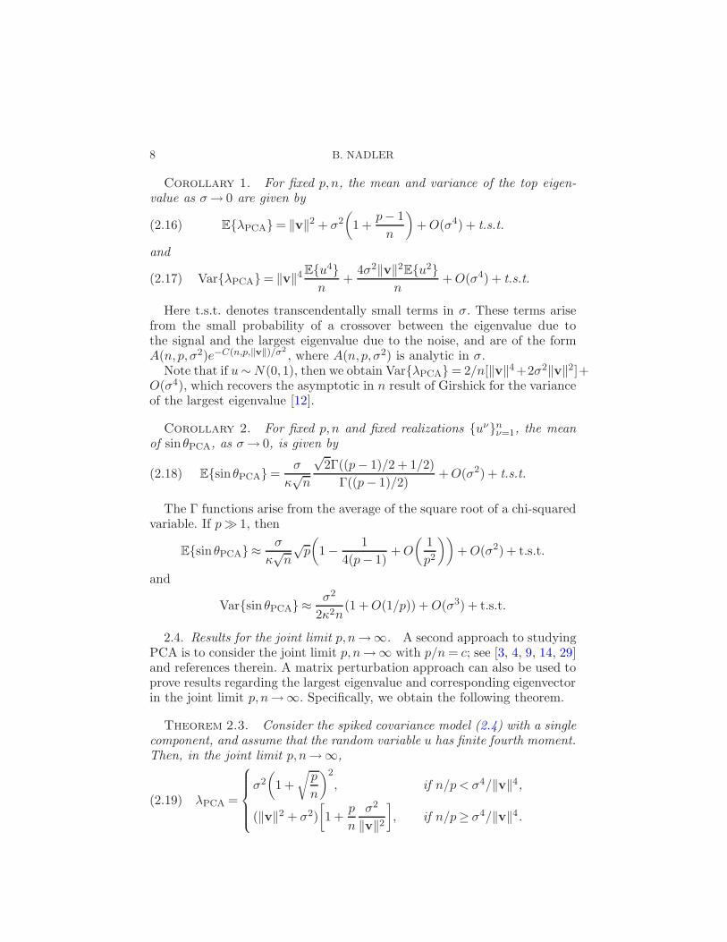
Corollary 1. For fixed p,n, the mean and variance of the top eigen-value as σ → 0 are given by

E{λPCA}= ‖v‖2 + σ2(

1 +p− 1

n

)

+ O(σ4) + t.s.t.(2.16)

and

Var{λPCA}= ‖v‖4 E{u4}n

+4σ2‖v‖2

E{u2}n

+ O(σ4) + t.s.t.(2.17)

Here t.s.t. denotes transcendentally small terms in σ. These terms arisefrom the small probability of a crossover between the eigenvalue due tothe signal and the largest eigenvalue due to the noise, and are of the formA(n,p,σ2)e−C(n,p,‖v‖)/σ2

, where A(n,p,σ2) is analytic in σ.Note that if u ∼ N(0,1), then we obtain Var{λPCA} = 2/n[‖v‖4 +2σ2‖v‖2]+

O(σ4), which recovers the asymptotic in n result of Girshick for the varianceof the largest eigenvalue [12].

Corollary 2. For fixed p,n and fixed realizations {uν}nν=1, the mean

of sinθPCA, as σ → 0, is given by

E{sinθPCA}=σ

κ√

n

√2Γ((p− 1)/2 + 1/2)

Γ((p− 1)/2)+ O(σ2) + t.s.t.(2.18)

The Γ functions arise from the average of the square root of a chi-squaredvariable. If p ≫ 1, then

E{sinθPCA} ≈σ

κ√

n

√p

(

1− 1

4(p− 1)+ O

(

1

p2

))

+ O(σ2) + t.s.t.

and

Var{sin θPCA} ≈σ2

2κ2n(1 + O(1/p)) + O(σ3) + t.s.t.

2.4. Results for the joint limit p,n →∞. A second approach to studyingPCA is to consider the joint limit p,n→∞ with p/n = c; see [3, 4, 9, 14, 29]and references therein. A matrix perturbation approach can also be used toprove results regarding the largest eigenvalue and corresponding eigenvectorin the joint limit p,n→∞. Specifically, we obtain the following theorem.

Theorem 2.3. Consider the spiked covariance model (2.4) with a singlecomponent, and assume that the random variable u has finite fourth moment.Then, in the joint limit p,n→∞,

λPCA =

σ2

(

1 +

√

p

n

)2

, if n/p < σ4/‖v‖4,

(‖v‖2 + σ2)

[

1 +p

n

σ2

‖v‖2

]

, if n/p≥ σ4/‖v‖4.

(2.19)

FINITE SAMPLE APPROXIMATION RESULTS 9

Similarly, the dot product between the population eigenvector and theeigenvector computed by PCA also undergoes a phase transition,

R2(p/n) = |〈vPCA,v〉|2(2.20)

=

0, if n/p < σ4/‖v‖4,(n‖v‖4)/(pσ4)− 1

(n‖v‖4)/(pσ4) + (‖v‖2)/σ2, if n/p ≥ σ4/‖v‖4.

Equation (2.20) shows that to “learn” the direction of true largest vari-ance, even approximately, the ratio n/p must be larger than a critical thresh-old. This is named in the literature as retarded learning, or as the phase tran-sition phenomenon. In the statistical physics community these results werederived using the replica method [5, 37]. In the statistics literature (2.19) wasproven by Baik and Silverstein, using the Stieltjes transform [4], for the moregeneral case of a spiked covariance model with an arbitrary finite number ofindependent and not necessarily Gaussian components. They showed that(with σ = 1) all eigenvalues αj > 1 +

√

p/n are shifted to αj + cαj/(αj − 1),and stated that “it would be interesting to have a simple heuristic argument”which shows how to obtain these pulled up values. In this section we presenta matrix perturbation view of this problem, including a simple derivationof the pulled up values and some discussion as to the phenomenon for finitep,n. A similar approach was recently independently derived by Paul [31].

Equation (2.19) shows that for a spiked covariance model with a singlecomponent and with σ = 1, in the joint limit p,n→∞, a large enough signaleigenvalue α is shifted to

α +p

n

α

α− 1.(2.21)

We now present an interesting connection between this formula and a classicresult by Lawley from 1956. In [23], Lawley considered the eigenvalues ofPCA for multivariate Gaussian observations whose limiting covariance ma-trix is diagonal with eigenvalues α1, . . . , αp. Denote by ℓ1, . . . , ℓp the noisyeigenvalues of PCA corresponding to a sample covariance matrix with afinite number of samples n. Then, as n →∞, with p fixed

E{ℓk}= αk +αk

n

p∑

i=1,i6=k

αi

αk − αi+ O

(

1

n2

)

.(2.22)

Applying Lawley’s result to the spiked covariance model with a single sig-nificant component (α1 = α,α2 = · · ·= αp = 1) gives

λPCA = α +p− 1

n

α

α− 1+ O

(

1

n2

)

10 B. NADLER

whose first two terms recover the asymptotic result (2.21) of the joint limitp, n→∞. The remarkable point in using (2.22) is that it does not use ex-plicit knowledge of the Marchenko–Pastur distribution, regarding the lim-iting density of eigenvalues of infinitely large random matrices. We remarkthat although the first two terms in Lawley’s expansion provide the asymp-totic result as p,n →∞, this is not due to the higher-order terms all van-ishing individually. Rather, in the joint limit p,n→∞ they all miraculouslycancel each other. Yet, based on this observation, we propose the followingtwo theorems.

Theorem 2.4. Consider a more general Gaussian spiked covariancemodel with k large components with fixed variances α1, . . . , αk and with thep − k remaining components each having a random variance sampled inde-pendently from a density h(α) with compact support in the interval [0, αc](h(α) = 0 for α > αc). Then, in the joint limit p,n→∞ and for large enoughvalues αj , the first k largest limiting eigenvalues of PCA converge to

λj = T (αj) = αj +p

nαj

∫ αc

0

ρ

αj − ρh(ρ)dρ.(2.23)

Theorem 2.5. Let {αj} denote an infinite sequence of i.i.d. randomvariables from a density h(α) with compact support. Let x = (x1, . . . , xp) bea p-dimensional vector composed of p independent Gaussian random vari-ables, where each xj has variance αj . Let C(n,p) denote the p× p empiricalcovariance matrix computed from n independent samples {xi}n

i=1 from thismodel. Then, in the joint limit p,n→∞, p/n = c, the spectral norm of C isequal to

limp,n→∞

‖C‖= α∗ + cα∗∫

ρ

α∗ − ρh(ρ)dρ(2.24)

where α∗ is the maximal point at which

dT (α)

dα

∣

∣

∣

α∗= 0.(2.25)

A motivation for the model considered in these theorems is a setting wherehigh-dimensional observations are of the type “signal plus noise,” but wherethe noise is heteroscedastic and possibly correlated. Thus, in a suitable basis,different noise components have different variances, and we only know somestatistical properties about the noise, such as the distribution of these vari-ances. Theorem 2.4 is a generalization of (2.21) that holds for the standardspiked covariance model. Theorem 2.5 follows immediately from Theorem2.4 according to the following reasoning: In this modified model there isalso a similar phase transition phenomenon. If the original variance of the

FINITE SAMPLE APPROXIMATION RESULTS 11

signal, α, is larger than a critical value α∗(h, p,n), then it will be pulled upfrom the noise in the limit p,n →∞. Further, for all α > α∗, this pulled upvalue is monotonic in α. From Theorem 2.4, the critical value α∗ satisfies(2.25), and at that point according to our matrix perturbation analysis, thevalue T (α∗) is equal to the spectral norm C—the covariance matrix of thenoise. We remark that a formula similar to (2.24) was recently derived by ElKaroui [11], who also studied the finite p,n fluctuations around this mean.

Corollary 3. Consider the general spiked covariance model as in The-orem 2.4, and assume c = p/n ≫ 1. Let

µ1 =

∫

ρh(ρ)dρ, µ22 =

∫

(ρ− µ1)2h(ρ)dρ.

Then, in the joint limit p,n →∞, the norm of a pure noise matrix is ap-proximately

λ(α∗) = µ1

(

c + 2√

c

√

1 +µ2

2

µ21

+ O(1)

)

.(2.26)

Further, the phase transition phenomenon for the pulled up eigenvalues oc-curs at

α∗ = µ1

(√c

√

1 +µ2

2

µ21

+ 1 + 4µ2

2/µ21

1 + 2µ22/µ

21

+ O(1/√

c)

)

.(2.27)

Equation (2.26) may be useful for inference on the number of componentsin a general spiked covariance model, given that the first two moments µ1, µ2

of the density h(ρ) of the noise are either known a priori or estimated fromthe data.

3. Proof of Theorem 2.1. To prove Theorem 2.1 we shall use the follow-ing three lemmas:

Lemma 1. Let A,B be p × p Hermitian matrices. Let {λi}pi=1 denote

the eigenvalues of A sorted in decreasing order with corresponding eigen-vectors vi. Let Pi denote the projection into the orthogonal subspace of vi,Piv = v− 〈v,vi〉vi. If λ1 has multiplicity 1 and ‖B‖< λ1 + 〈v1,Bv1〉 − λ2,then the largest eigenvalue of A + B satisfies the bounds

〈v1,Bv1〉 ≤ λ1(A + B)− λ1 ≤ 〈v1,Bv1〉+ ‖P1Bv1‖.(3.1)

Lemma 2. Let X denote an n × p matrix with entries Xij all i.i.d.N(0,1) Gaussian variables, and let W = XT X/n be the corresponding scaledWishart matrix. Define

ε = exp

(

− p

2(√

5 + 2)2

)

,(3.2)

12 B. NADLER

then for n ≤ p with probability at least 1− ε,

‖W‖ ≤ (1 +√

p/n)2 + p/n(3.3)

and

‖W − Ip‖ ≤ 4p

n.(3.4)

Lemma 3. Let A be a p× p Hermitian matrix and let B be a Hermitianperturbation. Let (λ,v) be the eigenvalue/vector pair of A + B correspond-ing to (λi,vi) of A, and let δ = minj 6=i |λ − λj|, where {λj}p

j=1 are all theeigenvalues of A; then

sinθ(v,vi)≤‖B‖

δ.(3.5)

Lemma 1 follows from classical results in matrix or operator perturbationtheory. According to [30], Theorem 4.5.1 (see also [13], Theorem 6.3.14), foreach scalar µ, vector x and Hermitian matrix A, there exists an eigenvalueλ of A such that

|λ− µ| ≤ ‖Ax− µx‖/‖x‖.

Applying this theorem to the matrix A+B, with x = vi a normalized eigen-vector of A and with µ = λi + 〈vi,Bvi〉, gives that

|λ(A + B)− λi(A)− 〈vi,Bvi〉| ≤ ‖PiBvi‖.

The condition of Lemma 1 ensures that the largest eigenvalue of A is theone closest to the largest eigenvalue of A + B, for example, i = 1. For theanalysis of a spiked covariance model with more than one component, sim-ilar statements can be made for interior eigenvalues as well [16]. Lemma 2follows from Theorem II.13 of Szarek and Davidson [7] and is proved in theAppendix. Lemma 3 is known as the sinθ theorem of Davis and Kahan [8];see also [30], Theorem 11.7.1.

Proof of Theorem 2.1. Let {xν}nν=1 be n i.i.d. observations from

the one-component model (2.4). We decompose the corresponding samplecovariance matrix as follows:

Sn =

κ2 0 · · · 00 0 0...

...0 0 · · · 0

+ σκ

2ρ1 ρ2 · · · ρp

ρ2 0 0... 0

...ρp 0 0

FINITE SAMPLE APPROXIMATION RESULTS 13

+ σ2

β1,1 β1,2 · · · β1,p

β2,1 β2,2...

.... . .

βp,1 · · · βp,p

(3.6)

= L0 + σL1 + σ2L2,

where κ,ρj and βij are defined above in (2.6) and (2.7). Note that conditionalon the realizations {uν}n

ν=1 of the random variable u kept fixed, ρi = 1√nηi,

where ηi are all i.i.d. N(0,1), βii = χ2n/n and that L2 is a Wishart noise

matrix. The matrix L0 can be thought of as the “signal,” the matrix L1 asthe signal–noise interactions, whereas L2 contains pure noise.

To derive the lower bound (2.11), we view the matrix σ2L2 as a pertur-bation of the matrix L0 + σL1. Since the matrix L2 is nonnegative (it is ascaled Wishart matrix), it follows that

λPCA ≥ ‖L0 + σL1‖.

The matrix L0 +σL1 has rank 2 with the following two nonzero eigenvalues:

λ± =(κ2 + 2σκρ1)±

√

(κ2 + 2σκρ1)2 + 4(σκ)2∑

j≥2 ρ2j

2,(3.7)

where λ+ is positive and λ− is negative. Since conditional on the realizationsuν fixed, the random variables ρj are independent Gaussians, we define

∑

j≥2

ρ2j =

T1

n,(3.8)

where T1 ∼ χ2p−1.

Using the inequality√

1 + x ≥ (1 + x/2− x2/8) in (3.7) gives

λ+ ≥ (κ2 + 2σκρ1)

[

1 +σ2κ2

(κ2 + 2σκρ1)2T1

n− (σκ)4

(κ2 + 2σκρ1)4T 2

1

n2

]

.

Therefore, with probability at least 1− ε1 − ε2

λPCA ≥ λ+ ≥ κ2(

1− 2σs1

κ√

n

)[

1 +σ2

κ2

p− 1

n

1− s2/√

p− 1

1 + (2σs1)/(κ√

n)

− σ4

κ4

(p− 1)2

n2

(1 + s2/√

p− 1)2

(1− (2σs1)/(κ√

n))3

]

,

which proves the lower bound (2.11).To prove the upper bound on λPCA, we use Lemma 1 with the matrix

σL1 + σ2L2 as a perturbation of L0. Choosing e1 as an eigenvector of L0

14 B. NADLER

and applying the lemma gives that

λPCA ≤ κ2 + 2σκρ1 + σ2β11 + σ√

∑

j≥2

(κρj + σβ1j)2.

Conditional on fixed realizations uν and on fixed noise realizations ξν1 in the

first component of the data, we have that

κρj + σβ1j =1√n

√

κ2 + 2σκρ1 + σ2β11ηj ,

where the ηj are independent standard Gaussian variables. Therefore,

λPCA ≤ (κ2 + 2σκρ1 + σ2β11) + σ√

κ2 + 2σκρ1 + σ2β11

√

T

n,

where the random variable T ∼ χ2p−1, and is independent of ρ1 and β11.

Therefore, with probability at least 1− ε− ε1 − ε2 − ε3 the bound of (2.12)follows.

To prove a bound on the eigenvector vPCA, we start from the eigenvectorv+ corresponding to λ+, and given by

v+ =1

Z

[

e1 +σκ

λ+(0, ρ2, . . . , ρp)

T]

,(3.9)

where Z =√

1 + σ2κ2T1/nλ2+ is a normalization constant such that ‖v+‖=

1.Simple algebraic manipulations and the triangle inequality give

sinθPCA =√

1− 〈vPCA,e1〉2 =√

1 + |〈vPCA,e1〉|√

1− |〈vPCA,e1〉|

=√

1 + |〈vPCA,e1〉|‖vPCA − e1‖√

2(3.10)

≤ ‖vPCA − e1‖ ≤ ‖vPCA − v+‖+ ‖v+ − e1‖.From (3.9), a bound on the second term in (3.10) is

‖v+ − e1‖ =√

2

√

1− 1

Z≤ σκ

λ+

√

T1

n.(3.11)

For the first term in (3.10), applying the sinθ theorem (Lemma 3 above) withthe matrix σ2(W − Ip) = σ2(L2 − Ip) as the perturbation of L0 +σL1 +σ2Ip

gives

‖vPCA − v+‖ =√

2√

1− |〈vPCA,v+〉| ≤√

2 sinθ(vPCA,v+)(3.12)

≤√

2σ2 ‖W − Ip‖δ

,

FINITE SAMPLE APPROXIMATION RESULTS 15

where δ = minj 6=1 |λPCA−λj(L0 +σL1 +σ2Ip)|. Therefore, combining (3.11)and (3.12),

sin θPCA ≤ σκ

λ+

√

T1

n+ σ2

√2‖W − Ip‖

δ.(3.13)

To conclude the proof we apply almost sure bounds for ‖W − Ip‖ and T1

from above and δ and λ+ from below. Bounds on T1 and λ+ are identical tothose described in the proof of (2.11) of the theorem. To bound ‖W − Ip‖from above, we use (3.4) of Lemma 2, which states that with probability atleast 1− ε

‖W − Ip‖ ≤ 4p

n.(3.14)

As for a bound on δ, from the first part of the proof, if κ2 +2σκρ1 > σ2[(1+√

p/n)2 + p/n],

λPCA ≥ λ+ ≥ κ2 + 2σκρ1.

Furthermore, the eigenvalues of the matrix L0 +L1 + σ2I are (λ+) + σ2, σ2

or (λ−) + σ2, with λ± given by (3.7). Therefore,

δ = minj 6=1

|λPCA − λj(L0 +L1 + σ2I)|= λPCA − σ2 ≥ κ2 + 2σκρ1 − σ2

and with probability at least 1− ε1,

δ ≥ κ2 − 2s1σκ√

n− σ2.(3.15)

Combining (3.13), (3.14) and (3.15) concludes the proof. �

4. Proof of Theorem 2.2. We now explore the leading order terms in σof the explicit dependence of λPCA and vPCA on p,n, and on the specificsignal and noise realizations {uν}n

ν=1 and {ξν}nν=1. To this end, we view σ

as a small parameter and consider the Taylor expansion of λPCA and vPCA

as σ → 0. By definition, the largest eigenvalue λPCA is the largest root ofthe characteristic polynomial of sample covariance matrix Sn. For σ = 0this eigenvalue is a simple root with multiplicity 1. Therefore, given a finitedataset {xν}n

ν=1 with su > 0, the largest eigenvalue λ(σ), when viewed asa function of noise level, is an analytic function of σ in the complex planefor small enough σ. This statement follows from the representation of theempirical covariance matrix as Sn =L0 + σL1 + σ2L2, (3.6), with all matri-ces being symmetric, together with standard results regarding perturbationtheory for linear operators; see, for example, Kato [21], Chapter 2, Theo-rem 6.1. Moreover, the radius of convergence of a Taylor series of λ(σ) isthe largest complex σ for which λPCA(σ) > λ2(σ) where λ2(σ) is the second

16 B. NADLER

largest eigenvalue of the noisy covariance matrix. Note that the location ofthe crossover depends on the specific signal and noise realizations. Finally,since the matrix Sn is symmetric λ(σ) is real when σ is real.

Therefore, for small enough σ we can expand both the top eigenvalue andits corresponding eigenvector as a regular power series in σ:

vPCA = v0 + σv1 + σ2v2 + · · · ,

λPCA = λ0 + σλ1 + σ2λ2 + · · · .We insert these expansions into (3.6) and equate terms with equal powersof σ. The first few equations read

L0v0 = λ0v0,

L0v1 +L1v0 = λ0v1 + λ1v0,

L0v2 +L1v1 +L2v0 = λ0v2 + λ1v1 + λ2v0.

Iteratively solving these equations gives

λ = κ2 + 2σκρ1 + σ2

(

∑

j≥2

ρ2j + β11

)

+ O(σ3)(4.1)

and

v = e1 +σ

κ(0, ρ2, . . . , ρp)

(4.2)

+σ2

κ2[(0, β12, . . . , β1p)− 2ρ1(0, ρ2, . . . , ρp)] + O

(

σ3

κ3

)

.

Note that up to order O(σ2), the eigenvalue λPCA and the correspondingeigenvector depend only on the first row of the noisy matrix, for example,only on the interaction between signal and noise.

Equations (2.16), (2.17) and (2.18) follow by taking expectations on ex-pressions (4.1) and (4.2) for λPCA and vPCA, respectively, and retaining onlythe leading terms in σ. However, an important remark is that (4.1) and (4.2)are the Taylor expansions of the eigenvalue and eigenvector that are ana-lytic in σ and correspond to κ2 and e1 when σ = 0. As such, these are notnecessarily expansions of λPCA and vPCA—the actual largest eigenvalue andcorresponding eigenvector of the sample covariance matrix. This is becausefor finite σ > 0 there is a nonzero probability that the largest eigenvalue isone due to noise and not the one described by (4.1). From Lemma 2, theprobability of such a crossover, between the eigenvalue due to noise andthe eigenvalue due to the signal, can be bounded by an expression of theform A(n,p) exp(−C(n,p)/σ2). Therefore, by taking expectations of (4.1),we introduce transcendentally small error terms in σ.

FINITE SAMPLE APPROXIMATION RESULTS 17

5. Proof of Theorem 2.3: the phase transition phenomenon.

5.1. A simple heuristic for the location of the phase transition. First, wepresent a simple heuristic explanation for the phase transition phenomenon,but for fixed p,n, as a function of noise level σ. Obviously, for fixed p,nthere is no deterministic phase transition at a fixed constant c = p/n, onlyan increasing probability for losing the relation between the direction ofmaximal variance and the limiting vector e1. From the analysis of Section3, this occurs when the largest eigenvalue of the sample covariance matrix isof the same order of magnitude as that of the noise matrix E, λPCA ∼ ‖E‖.From (3.4), this occurs roughly when

κ2 + σ2 + σ2 p

n= σ2(1 +

√

p/n)2.

This gives

p

n=

1

4

κ4

σ4,

which up to a multiplicative constant has the same functional dependenceon the parameters p,n,σ as the true location for the phase transition in(2.19) and (2.20).

5.2. An exact analysis of the phase transition. We now present a sim-ple linear-algebra based derivation of the exact pulled up value for a spikedpopulation model with a single component. A similar though more compli-cated analysis applies for the general k-component model. For simplicity, weperform our analysis for p/n = c = 1, and without loss of generality assumeσ = 1.

To this end, we decompose the p× p sample covariance matrix computedfrom n samples as follows:

Sn =

κ2 + 2κρ11 + β11 b2 · · · bp

b2 0 · · · 0...

.... . .

...bp 0 · · · 0

+

0 0 · · · 00 β22 · · · β2p... β32

. . . β3p

0 βp2 · · · βpp

,

where bj = κρj +β1j . Note that the second matrix, which is the minor of thecovariance matrix obtained by deleting the first row and column, is just a(p− 1)× (p− 1) scaled Wishart matrix. Let λ2, . . . , λp denote its eigenvaluesand let Vp×p be the matrix of its eigenvectors padded with zeros in thefirst coordinate. We perform a change of basis whereby this matrix becomesdiagonal. Then the full covariance matrix takes the following form:

V SnV T =

κ2 + 2κρ1 + β11 b2 · · · bp

b2 λ2 · · · 0...

.... . .

...bp 0 · · · λp

,(5.1)

18 B. NADLER

where b1j are the entries of the first row and column in the new basis. Thespecific form (5.1) is known as an arrowhead matrix [28]. Assuming thatbj 6= 0 for all j (an event with probability 1), the eigenvalues of this matrixsatisfy the following secular equation:

f(λ) = (λ− κ2 − 2κρ1 − β11)−p∑

j=2

b2j

λ− λj= 0.(5.2)

Recall that bj = ρj + β1j are the entries of the first row and column in thenew basis. They are given explicitly as

ρj =1

nsy

n∑

ν=1

uνj ξ

νj , β1j =

1

n

n∑

ν=1

ξν1 ξν

j ,

where ξν are the noise vectors in the rotated basis in which the (p− 1)× (p− 1)submatrix of noise covariances is diagonal with eigenvalues λj . Therefore,

conditional on ξj having variance λj , the quantity bj is N(0, λj(κ2 + 2κρ1 +

β11)/n). Therefore,

p∑

j=2

b2j

λ− λj=

p− 1

n(κ2 + 2κρ + β11)

1

p− 1

p∑

j=2

λjη2j

λ− λj,

where ηj are all i.i.d. N(0,1) and independent of λj . Furthermore, in thelimit p,n→∞, p/n = c, the distribution of eigenvalues λj of the submatrixconverges to the Marcenko–Pastur distribution [24],

fMP(x) =1

2πxc

√

(b− x)(x− a), x ∈ [a, b],

where a = (1 − √c)2, b = (1 +

√c)2. In addition, as n,p → ∞, κ2 → ‖v‖2,

ρ1 = OP (1/√

n) → 0 and β11 = χ2n/n → 1, all with probability 1. Therefore,

as p,n→∞, the sum in (5.2) converges with probability 1 to the followingintegral:

limp,n→∞

p∑

j=2

b2j

λ− λj= (‖v‖2 + 1)

p− 1

n

∫ b

afMP(x)

x

λ− xdx.(5.3)

This integral is a linear functional of the Marcenko–Pastur distribution,with some similarity to its Stieltjes transform. We remark that the Stieltjestransform was used extensively in deriving results regarding the eigenvaluesof random matrices [24, 33].

This integral can be evaluated explicitly. For example, for c = 1,∫ 4

0

1

2π

√

(4− x)x1

λ− xdx =

1

2[λ− 2−

√

λ(λ− 4)].(5.4)

FINITE SAMPLE APPROXIMATION RESULTS 19

Thus, the largest eigenvalue satisfies a quadratic equation in λ, whose solu-tion is

λ(α) = α + cα

α− 1

with α = ‖v‖2 + 1. However, this solution is indeed the largest eigenvalueonly if λ(α) > (1 +

√c)2. This recovers the pulled up value and the exact

location of the phase transition, (2.19).To prove (2.20) for the eigenvector overlap, we note that eigenvectors of

arrowhead matrices have also a closed form expression [28]. Let λ be aneigenvalue of the arrowhead matrix (5.1); then up to normalization, thecorresponding eigenvector is given by

v =

(

1,b2

λ− λ2, . . . ,

bp

λ− λp

)

.(5.5)

Therefore,

R2 =〈v,e1〉2‖v‖2

=1

1 +∑

j≥2 b2j/(λ− λj)2

.

In the joint limit p,n → ∞, similar to the analysis above, the sum in thedenominator converges with probability 1 to an analogous integral

limp,n→∞,p/n=c

R2 =1

1 + p/n∫

αµ/(λ− µ)2fMP(µ)dµ.(5.6)

Evaluation of the integral gives the asymptotic overlap, (2.20).

5.3. A classical result of Lawley and two theorems. While Theorems2.4 and 2.5 are motivated by the classical result of Lawley, (2.22), theirproof relies on results from random matrix theory regarding the limitingempirical density of eigenvalues of sample covariance matrices in the jointlimit p,n →∞. Before proving these theorems, we first briefly review theresults required for our proofs.

The key required quantity is the Stieltjes transform of a probability den-sity h(t) defined as

mh(z) =

∫

h(t)

t− zdt ∀z ∈ C

+.(5.7)

Let Sn = 1/nZT Z be the p×p sample covariance matrix of n observationszi ∈ R

p from the model described in Theorem 2.5, and denote by Fn theempirical distribution function of the eigenvalues of Sn,

Fn(t) ={#µj < t}

p.(5.8)

20 B. NADLER

As proven in [33], in the limit p,n→∞, Fn converges with probability 1 to alimiting distribution F with no eigenvalues of Sn outside the support of thislimiting distribution. Although the explicit form of F can be computed onlyin a handful of simple cases, its Stieltjes transform satisfies the equation

m(z) =

∫

h(t)

t(1− c−m(z)z)− zdt.(5.9)

One can also consider a different matrix, Sn = 1/nZZT of size n× n. Sincethe matrices Sn and Sn have the same nonzero eigenvalues and differ by|p − n| zero eigenvalues, their respective empirical distribution functions Fand F are related as follows:

F = (1− c)I[0,∞) + cF.

Due to linearity of the Stieltjes transform,

m(z) = −1− c

z+ cm(z).(5.10)

Obviously, when c = 1, m(z) = m(z).The last result of interest is an inverse equation for m(z), which reads

z(m) =− 1

m+ c

∫

t

1 + tmh(t)dt.(5.11)

Proof of Theorem 2.4. For simplicity, we consider a spiked covari-ance model with a single spike, assumed in the direction e1. Let α1 be fixedand sufficiently large, and let {αj}j≥2 denote a sequence of i.i.d. realizationssampled from a density h(α). Consider n i.i.d. random vectors {xν}n

ν=1 froma model

x =√

α1y1e1 +p∑

j=2

√αjyjej ,

where yj are all i.i.d. Gaussian N(0,1) random variables. We view the direc-tion e1 as the signal direction with all other directions as noise, and writethe corresponding sample covariance matrix as follows:

Sn =

κ2 b1 · · · bp

b1... Cn

bp

,

where

κ2 =1

n

n∑

ν=1

(xν1)

2, bj =1

n

n∑

ν=1

xν1x

νj

FINITE SAMPLE APPROXIMATION RESULTS 21

and Cn is the (p − 1) × (p − 1) sample covariance matrix of the pure noisecomponents.

Let V0 be a (p − 1) × (p − 1) matrix that diagonalizes the pure noisematrix Cn, and consider the p× p unitary matrix

V =

(

1V0

)

.

In the basis defined by V , the sample covariance matrix takes the form

V SnV −1 =

κ2 b1 b2 · · · bp

b1 µ1

b2 µ2...

. . .

bp µp

,(5.12)

where bj is the projection of the vector b on the jth basis vector of thematrix V ,

bj = bT Vj =

1

n

n∑

ν=1

xν1x

νj .

As in (5.1), the matrix (5.12) has the form of a symmetric arrowhead matrix,and assuming all bj 6= 0, its eigenvalues are solutions of

λ− κ2 =p∑

j=1

b2j

λ− µj.(5.13)

We now consider the joint limit p,n→∞, p/n = c. Similarly to the analysisof Section 5.2, the sum in (5.13) converges with probability 1 to

cα1

∫

µ

λ− µdF (µ),(5.14)

where F (µ) is the limiting probability distribution of a pure noise randommatrix corresponding to the density h(α). Therefore, the pulled up value isthe solution of

λ− α1 = cα1

∫

µ

λ− µdF (µ).(5.15)

To finish the proof, we use Lemma 4 below, which shows that for any valueof c and density h, m(λ(α)) = −1/α, and then insert this relation into theinverse equation (5.11). �

Lemma 4. Let λ(α) denote the pulled up value corresponding to an orig-inal eigenvalue α. For α large enough, regardless of the constant c and ofthe underlying density h(t),

m(λ(α)) =− 1

α.(5.16)

22 B. NADLER

Proof. We rewrite (5.15) as follows:

λ(α) = α(1− c) + λαc

∫

1

λ− µdF (µ).(5.17)

By extending the definition of the Stieltjes transform m(z) of F , originallydefined only for z ∈ C

+, also to z ∈ R with z > support(F ), the last equationreads

λ(α) = α(1− c)− λαcm(λ(α))(5.18)

or stated otherwise

cm(λ(α)) − 1− c

λ(α)= − 1

α,(5.19)

but according to (5.10), the left-hand side is simply m(λ(α)), also extendedto the case of inputs z ∈ R with z > support(F ). �

Proof of Theorem 2.5. We consider the relation α(λ). That is, foreach λ > support(F ) we look for the corresponding α such that (2.23) is sat-isfied. We show that there exists a unique solution α(λ), which is monotonicin λ, and as λ → support(F ), satisfies that α(λ) → α∗ <∞, but dα/dλ →∞.

To this end, we rewrite (5.17) as follows:

α =1

(1− c)/λ + c∫

1/(λ − µ)dF (µ).(5.20)

Since for λ > support(F ) the functions 1/λ and∫

1/(λ − µ)dF (µ) are bothstrictly monotonically decreasing in λ, it follows that

dα

dλ> 0 for λ > support(F ).(5.21)

We now analyze the behavior of both α(λ) and its derivative as λ approachesthe support of F . According to [9, 34] near the boundary b = support(F ),the density F exhibits a behavior closely resembling

√

|b− x|. Therefore,

limλ→support(F )

∫

1

λ− µdF (µ) = Const,(5.22)

whereas

limλ→support(F )

d

dλ

∫

1

λ− µdF (µ) =∞.(5.23)

This proves Theorem 2.5. �

Proof of Corollary 3. We start our analysis from the equation

λ(α) = α(1− c) + α2c

∫

h(t)

α− tdt.(5.24)

FINITE SAMPLE APPROXIMATION RESULTS 23

First we make a change of variables t = µ1 + s, where

µ1 =

∫

th(t)dt(5.25)

and denote h0(s) = h(t), with the subscript zero denoting the fact that thisdensity has zero mean. Then,

λ(α) = α(1− c) +α2c

α− µ1

∫

h0(s)

1− s/(α− µ1)ds.(5.26)

As c →∞, both α →∞ and λ →∞. Specifically, α − µ1 > support(F ). Inthis case we can expand

1

1− s/(α− µ1)=

∞∑

k=0

(

s

α− µ1

)k

,

where the sum is convergent for |s| < support(F ). Inserting this expansioninto (5.24) gives

λ(α) = α(1− c) +α2c

α− µ1

[

1 +

∫

s2h0(s)

(α− µ1)2ds + O

(

1

α− µ1

)3]

.(5.27)

Taking only the first two terms in the expansion gives the approximatesolution

α∗ = µ1(1 +√

c).

To obtain the correction due to the variance of the distribution, we expand

α∗ = µ

(

β1

√c + β0 +

β−1√c

+ · · ·)

(5.28)

and insert the expansion into (5.27). This gives

α∗ = µ

(√c

√

1 +µ2

2

µ21

+ 1 + 4µ2

2/µ21

1 + 2µ22/µ

21

+ O

(

1√c

))

(5.29)

for the location of the phase transition, and

λ(α∗) = µ

[

c + 2√

c

√

1 +µ2

2

µ21

+ O(1)

]

.(5.30)�

5.4. The phase transition phenomenon for finite p,n. We conclude bypresenting two examples of the phase transition phenomenon for the stan-dard spiked covariance model with finite p,n. In Figure 1 we present anexample of this phenomenon with n = 50, p = 200, κ = 2.8. For small noiselevel σ, the largest eigenvalue is roughly κ2 = 7.87, and 〈vPCA,e1〉 ≈ 1. Asthe noise level σ increases the dot product decreases smoothly. However, at a

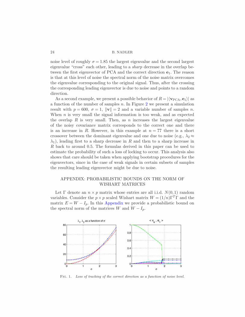
24 B. NADLER

noise level of roughly σ = 1.85 the largest eigenvalue and the second largesteigenvalue “cross” each other, leading to a sharp decrease in the overlap be-tween the first eigenvector of PCA and the correct direction e1. The reasonis that at this level of noise the spectral norm of the noise matrix overcomesthe eigenvalue corresponding to the original signal. Thus, after the crossingthe corresponding leading eigenvector is due to noise and points to a randomdirection.

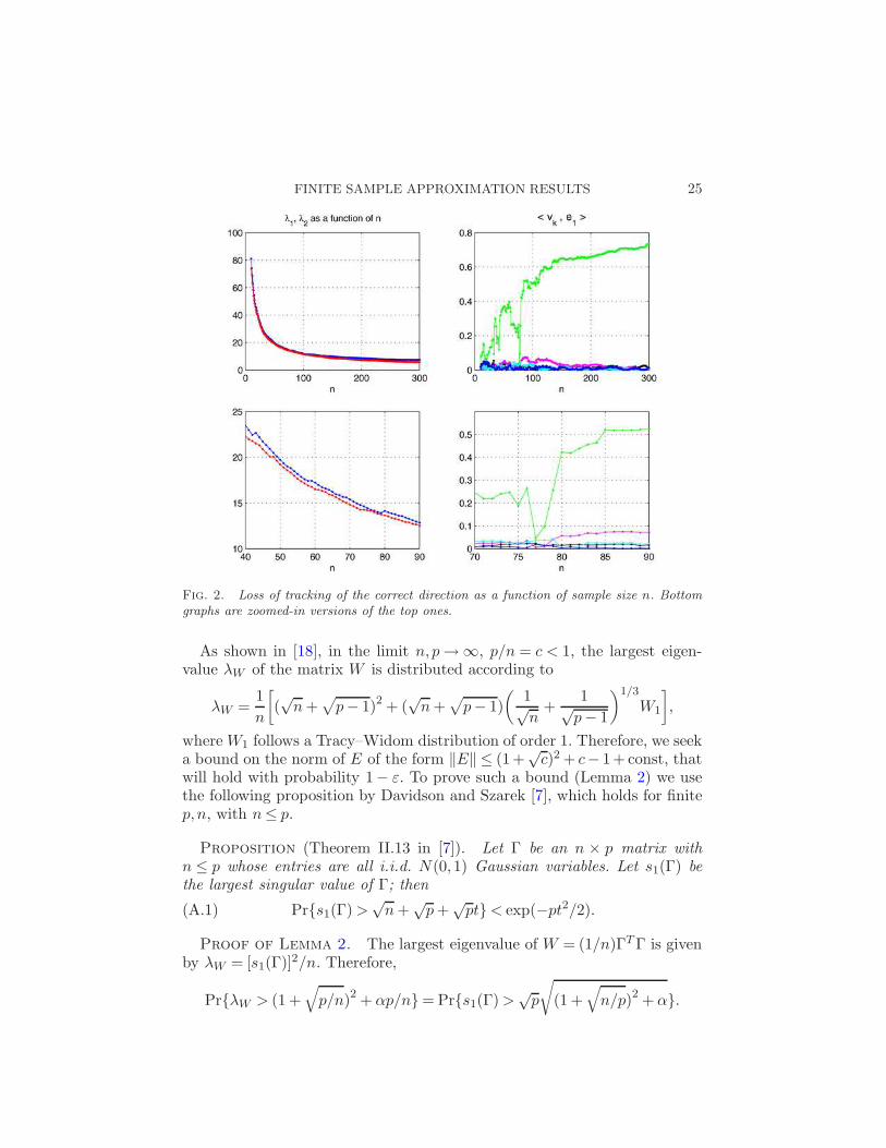
As a second example, we present a possible behavior of R = |〈vPCA,e1〉| asa function of the number of samples n. In Figure 2 we present a simulationresult with p = 600, σ = 1, ‖v‖ = 2 and a variable number of samples n.When n is very small the signal information is too weak, and as expectedthe overlap R is very small. Then, as n increases the largest eigenvalueof the noisy covariance matrix corresponds to the correct one and thereis an increase in R. However, in this example at n = 77 there is a shortcrossover between the dominant eigenvalue and one due to noise (e.g., λ2 ≈λ1), leading first to a sharp decrease in R and then to a sharp increase inR back to around 0.5. The formulas derived in this paper can be used toestimate the probability of such a loss of locking to occur. This analysis alsoshows that care should be taken when applying bootstrap procedures for theeigenvectors, since in the case of weak signals in certain subsets of samplesthe resulting leading eigenvector might be due to noise.

APPENDIX: PROBABILISTIC BOUNDS ON THE NORM OFWISHART MATRICES

Let Γ denote an n × p matrix whose entries are all i.i.d. N(0,1) randomvariables. Consider the p× p scaled Wishart matrix W = (1/n)ΓT Γ and thematrix E = W − Ip. In this Appendix we provide a probabilistic bound onthe spectral norm of the matrices W and W − Ip.

Fig. 1. Loss of tracking of the correct direction as a function of noise level.

FINITE SAMPLE APPROXIMATION RESULTS 25

Fig. 2. Loss of tracking of the correct direction as a function of sample size n. Bottom

graphs are zoomed-in versions of the top ones.

As shown in [18], in the limit n,p →∞, p/n = c < 1, the largest eigen-value λW of the matrix W is distributed according to

λW =1

n

[

(√

n +√

p− 1)2 + (√

n +√

p− 1)

(

1√n

+1√

p− 1

)1/3

W1

]

,

where W1 follows a Tracy–Widom distribution of order 1. Therefore, we seeka bound on the norm of E of the form ‖E‖ ≤ (1+

√c)2 + c− 1+ const, that

will hold with probability 1− ε. To prove such a bound (Lemma 2) we usethe following proposition by Davidson and Szarek [7], which holds for finitep,n, with n≤ p.

Proposition (Theorem II.13 in [7]). Let Γ be an n × p matrix withn ≤ p whose entries are all i.i.d. N(0,1) Gaussian variables. Let s1(Γ) bethe largest singular value of Γ; then

Pr{s1(Γ) >√

n +√

p +√

pt}< exp(−pt2/2).(A.1)

Proof of Lemma 2. The largest eigenvalue of W = (1/n)ΓT Γ is givenby λW = [s1(Γ)]2/n. Therefore,

Pr{λW > (1 +√

p/n)2 + αp/n}= Pr{s1(Γ) >√

p

√

(1 +√

n/p)2 + α}.

26 B. NADLER

We write

√p

√

(1 +√

n/p)2 + α =√

n +√

p +√

pt

with

t =

√

(1 +√

n/p)2 + α− (1 +√

n/p)

and use (A.1) to obtain that

Pr{λW > (1 +√

p/n)2 + αp/n}

≤ exp

[

−p

2(

√

α + (1 +√

n/p)2 − (1 +√

n/p))2]

(A.2)

≤ exp

[

−p

2

(

α√

α + (1 +√

n/p)2 + 1 +√

n/p

)2]

.

We specifically consider α = 1. Then, since n ≤ p,

1√

1 + (1 +√

n/p)2 + 1 +√

n/p≥ 1√

5 + 2(A.3)

and

Pr{λW > (1 +√

p/n)2 + p/n} ≤ exp

{

− p

2(√

5 + 2)2

}

= ε.(A.4)

Similarly, for n/p≤ 1, with probability at least 1− ε,

‖E‖ = ‖W − I‖ ≤ (1 +√

p/n)2 +p

n− 1 ≤ 4

p

n.(A.5) �

Remark. For n < p the matrix ΓT Γ always has p−n eigenvalues equalto 0, therefore E has p−n eigenvalues equal to −1. Thus, to bound ‖E‖ weneed only bounds on the largest positive eigenvalue as analyzed above.

Acknowledgments. It is a pleasure to thank Iain Johnstone, Andrew Bar-ron, Ilse Ipsen, Ann Lee and Patrick Perry for interesting discussions anduseful suggestions. The author also acknowledges the anonymous refereesfor valuable criticism which greatly improved the exposition of the paper.

REFERENCES

[1] Anderson, T. W. (1963). Asymptotic theory for principal component analysis. Ann.

Math. Statist. 34 122–148. MR0145620[2] Anderson, T. W. (1984). An Introduction to Multivariate Statistical Analysis, 2nd

ed. Wiley, New York. MR0771294

FINITE SAMPLE APPROXIMATION RESULTS 27

[3] Baik, J., Ben Arous, G. and Peche, S. (2005). Phase transition of the largesteigenvalue for nonnull complex sample covariance matrices. Ann. Probab. 33

1643–1697. MR2165575[4] Baik, J. and Silverstein, J. W. (2006). Eigenvalues of large sample covariance

matrices of spiked population models. J. Multivariate Anal. 97 1382–1408.

MR2279680[5] Biehl, M. and Mietzner, A. (1994). Statistical-mechanics of unsupervised structure

recognition. J. Phys. A 27 1885. MR1280357[6] Buckheit, J. and Donoho, D. L. (1995). Improved linear discrimination using time

frequency dictionaries. Proc. SPIE 2569 540–551.

[7] Davidson, K. R. and Szarek, S. (2001). Local operator theory, random matrices andBanach spaces. In Handbook on the Geometry of Banach Spaces (W. B. Johnson

and J. Lindenstrauss, eds.) 1 317–366. North-Holland, Amsterdam. MR1863696[8] Davis, C. and Kahan, W. M. (1970). The rotation of eigenvectors by a perturbation.

III. SIAM J. Numer. Anal. 70 1–47. MR0264450

[9] Dozier, R. B. and Silverstein, J. W. (2007). On the empirical distribution ofeigenvalues of large-dimensional information-plus-noise type matrices. J. Multi-

variate Anal. 98 678–694. MR2322123[10] Eaton, M. and Tyler, D. E. (1991). On Wielandt’s inequality and its application

to the asymptotic distribution of the eigenvalues of a random symmetric matrix.

Ann. Statist. 19 260–271. MR1091849[11] El Karoui, N. (2007). Tracy–Widom limit for the largest eigenvalue of a large class

of complex sample covariance matrices. Ann. Probab. 35 663–714. MR2308592[12] Girshick, M. A. (1939). On the sampling theory of the roots of determinantal

equations. Ann. Math. Statist. 10 203–204. MR0000127

[13] Horn, R. A. and Johnson, C. R. (1990). Matrix Analysis. Cambridge Univ. Press.MR1084815

[14] Hoyle, D. C. and Rattray, M. (2003). PCA learning for sparse high-dimensionaldata, Europhys. Lett. 62 117–123.

[15] Hyvarinen, A., Karhunen, J. and Oja, E. (2001). Independent Component Anal-

ysis. Wiley, New York.[16] Ipsen, I. C. F. and Nadler, B. (2008). Refined perturbation bounds for eigenval-

ues of Hermitian and non-Hermitian matrices. SIAM J. Matrix Anal. Appl. Toappear.

[17] Jackson, J. D. (1991). A User’s Guide to Principal Components. Wiley.

[18] Johnstone, I. M. (2001). On the distribution of the largest eigenvalue in principalcomponents analysis. Ann. Statist. 29 295–327. MR1863961

[19] Johnstone, I. M. and Lu, A. Y. (2008). Sparse principal components analysis. J.

Amer. Statist. Assoc. To appear.[20] Jolliffe, I. T. (2002). Principal Component Analysis, 2nd ed. Springer, New York.

MR2036084[21] Kato, T. (1995). Perturbation Theory for Linear Operators, 2nd ed. Springer, Berlin.

MR1335452[22] Kritchman, S. and Nadler, B. (2008). Determining the number of components in

a factor model from limited noisy data. Chemom. Int. Lab. Sys. 94 19–32.

[23] Lawley, D. N. (1956). Tests of significance for the latent roots of covariance andcorrelation matrices. Biometrika 43 128–136. MR0078610

[24] Marcenko, V. A. and Pastur, L. A. (1967). Distribution for some sets of randommatrices. Math. USSR-Sb 1 457–483.

28 B. NADLER

[25] Nadler, B. and Coifman, R. R. (2005). Partial least squares, Beer’s law and thenet analyte signal: Statistical modeling and analysis. J. Chemometrics 19 45–54.

[26] Nadler, B. and Coifman, R. R. (2005). The prediction error in CLS and PLS: Theimportance of feature selection prior to multivariate calibration. J. Chemom. 19

107–118.[27] Naes, T., Isaksson, T., Fearn, T. and Davis, T. (2002). Multivariate Calibration

and Classification. NIR Publications, Chichester, UK.[28] O’Leary, D. P. and Stewart, G. W. (1990). Computing the eigenvalues and

eigenvectors of symmetric arrowhead matrices. J. Comput. Phys. 90 497–505.MR1071882

[29] Onatski, A. (2007). Asymptotic distribution of the principal components esti-mator of large factor models when factors are relatively weak. Available athttp://www.columbia.edu/˜ao2027/inference45.pdf.

[30] Parlett, B. N. (1980). The Symmetric Eigenvalue Problem. Prentice-Hall, Engle-wood Cliffs, NJ. MR0570116

[31] Paul, D. (2007). Asymptotics of sample eigenstructure for a large dimensional spikedcovariance model. Statist. Sinica 17 1617–1642. MR2399865

[32] Reimann, P., Van den Broeck, C. and Bex, G. J. (1996). A Gaussian scenariofor unsupervised learning. J. Phys. A 29 3521–3535.

[33] Silverstein, J. W. and Bai, Z. D. (1995). On the empirical distribution of eigen-values of a class of large-dimensional random matrices. J. Multivariate Anal. 54

175–192. MR1345534[34] Silverstein, J. W. and Choi, S. I. (1995). Analysis of the limiting spectral distri-

bution of large-dimensional random matrices. J. Multivariate Anal. 54 295–309.MR1345541

[35] Stewart, G. W. (1990). Stochastic perturbation theory. SIAM Rev. 32 579–610.MR1084571

[36] Stewart, G. W. (1991). Perturbation theory for the singular value decomposition.In SVD and Signal Processing II: Algorithms, Analysis and Applications (R. J.Vaccaro, ed.) 99–109.

[37] Watkin, T. H. and Nadal, J.-P. (1994). Optimal unsupervised learning. J. Phys.

A 27 1899–1915. MR1280358

Department of Computer Science

and Applied Mathematics

Weizmann Institute of Science

Rehovot 76100

Israel

E-mail: boaz.nadler@weizmann.ac.il