Optimal Static-Dynamic Hedges for Exotic Options under

Convex Risk Measures

Aytac Ilhan ∗ Mattias Jonsson † Ronnie Sircar ‡

April 8, 2008; revised February 6, 2009 and June 15, 2009

Abstract

We study the problem of optimally hedging exotic derivatives positions using a com-bination of dynamic trading strategies in underlying stocks and static positions in vanillaoptions when the performance is quantified by a convex risk measure. We establish condi-tions for the existence of an optimal static position for general convex risk measures, andthen analyze in detail the case of shortfall risk with a power loss function. Here we findconditions for uniqueness of the static hedge. We illustrate the computational challengeof computing the market-adjusted risk measure in a simple diffusion model for an optionon a non-traded asset.

1 Introduction

Many recent papers have analyzed the stochastic control problem of portfolio optimizationunder exponential utility:

supθ

E

[

−e−γ(VT −G)]

.

Here, given a filtered probability space (Ω,F ,F, P ), G is the bounded FT -measurable payoff

of a derivative security, VT =∫ T0 θt dSt is the terminal value of following a trading strategy θ

in some underlying stocks S, and γ > 0 is a risk-aversion coefficient. Typically, this problemis an intermediate step in finding the (seller’s) indifference price of the claim G. We refer, forinstance, to [8, 24] and the collection [6].

Recast as a hedging problem

infθ

1

γlog E

[

e−γ(VT −G)]

,

this can be viewed as to optimally hedge with respect to the so-called entropic risk measure

eγ(X) =1

γlog(

E[

e−γX])

, X ∈ L∞(P ). (1.1)

∗Mathematical and Computational Finance Group, 24-29 St Giles’, Oxford, OX1 3LB, UK.†Department of Mathematics, University of Michigan, Ann Arbor, MI 48109-1109. (mattiasj@umich.edu).‡(Corresponding author): Department of Operations Research & Financial Engineering, Princeton Univer-

sity, Sherrerd Hall, Princeton, NJ 08544 (sircar@princeton.edu). Tel: +1 609 258 2841; Fax: +1 609 2584363. Work partially supported by NSF grants DMS-0456195 and DMS-0807440.

1

Some nice properties of this functional eγ : L∞(P ) → R, namely monotonicity, translationinvariance and convexity have been adopted as axioms for the class of convex risk measuresproposed by Follmer & Schied [13] (see Definition 2.1 below). In moving away from theentropic risk measure to this more general class, while the axiomatic properties are kept,other convenient features may be sacrificed, especially in terms of analytical and computationaltractability.

Our goal here is to analyze a specific hedging problem (static-dynamic hedging of exoticoptions), which we found to be quite tractable under the entropic risk measure [20, 18, 19],under other convex risk measures, and specifically the shortfall risk measure.

Static-Dynamic Hedging of Exotic Options

Exotic options are non-standard options, which may be variations of standard (vanilla) callsand puts, like barrier options, or tailored according to clients’ needs. These options are mostlytraded in over-the-counter (OTC) markets. It is common to think of hedging strategies astrading the underlying stock and bank account appropriately. In continuous-time models, thehedging portfolio is re-balanced at every instant, and this type of hedging is called dynamichedging. There is an alternative approach to hedge exotic options, which is less known, calledstatic hedging. The idea of static hedging was introduced in [5] and it involves trading otherliquid options. Trading occurs at some start time and the initial position is held throughout,which is why these hedges are called static.

In our approach, the investor, who assesses the risks associated with his financial positionby a convex risk measure, chooses an optimal combined strategy. The static hedging compo-nent is buying or selling standard options at initiation, and the dynamic hedging componentis following a stock-bank account trading strategy which is re-balanced continuously duringthe life of the options. We allow the investor to trade the standard options only statically,whereas she can trade the underlying stock and bank account continuously because of i) thehigher transaction costs associated with option trading compared to stock and bond trading,and ii) lesser liquidity in derivatives markets, but we do not explicitly model either of thesefrictions here.

We will assume that the market is incomplete, therefore not all the risks are hedgeablethrough trading the underlying stock. If the market were complete, given sufficient initialcapital, all claims could be replicated by trading the stock dynamically, and any positionin the standard option could be synthesized with such a trading strategy. Static derivativeshedges do not add anything to dynamic hedges in complete markets, but of course they arevery valuable tools in realistic incomplete market models, where there may be risk factors thatcannot be eliminated just by dynamic trading of the underlying stock. Exotic options can bevulnerable to these risk factors, for example volatility risk. As standard options, in general,will also be exposed to similar risk factors, they can be exploited to hedge these risks. Byincorporating static hedges, we enlarge the set of feasible hedging strategies that the investorcan choose from and allow for a better hedging performance.

In Section 2, we set up the problem and give sufficient conditions on an abstract convexrisk measure for existence of an optimal static-dynamic hedge of the exotic options position.Uniqueness is related to strict convexity of a certain value function and it is not simple togive useful conditions for it in general; rather, we focus on a sub-class of convex risk measures.For practical purposes, it seems there are two concrete classes of convex-but-not-coherent risk

2

measures: the entropic risk measure related to exponential utility, and shortfall risk. (Thereare also risk measures with more abstract definitions in terms of, for example, their penaltyfunctions, or acceptance sets, or drivers of BSDEs; see [3, 22]). In Section 3, we analyze theproblem under shortfall risk measures, which are of the form

ρ(X) = inf

m ∈ R | E

[

1

p((−m−X)+)p

]

≤ ξ

, X ∈ L∞

for some ξ > 0 and p > 1. We establish a sufficient condition for uniqueness of an optimalstatic hedge, depending on whether a dual optimization problem is solved by an equivalent(martingale) measure. A simple one-period example suggests the condition is not necessary.

In Section 5, we look at the computational problem in the case of dynamic hedging of anoption on a non-traded asset in a diffusion model, and under a shortfall risk measure. In thiscase, passing to the conjugate in the threshold level makes the problem amenable to dynamicprogramming methods (Section 4), and we give a numerical solution of the associated HJBequation. We conclude in Section 6.

2 Problem Formulation & Analysis

We consider an investor who has x dollars along with a short position in an exotic option, withpayoff Ge, that matures at time T . The investor tries to minimize the risks due to this optionposition by trading the underlying stock and bonds dynamically, and vanilla options availablein the market statically. We denote the stock price process (St)0≤t≤T , and the payoffs of thevanilla options by G = (G1, . . . , Gn), and we assume that G and Ge are bounded. A possiblecombined trading strategy is identified by ((θt)0≤t≤T , λ) where θt is the number of underlyingassets held at time t and λ = (λ1, . . . , λn) denotes the number of options sold initially. Theinvestor assesses the risk of a given trading strategy and initial wealth by

ρ

(

−λ ·G−Ge +

∫ T

0θ dS + x+ λ · g

)

, (2.1)

where ρ is a convex risk measure, defined below, g = (g1, · · · , gn) is the market price vectorof G, and “·” denotes the the usual inner product on R

n. Here, we assume for simplicity thatthe vanilla options also mature at time T and that the market uses a linear pricing rule. Notethat λ takes values in R

n and its components can be negative to imply long positions in G.Our problem is the minimization of (2.1) over (θ, λ).

2.1 Convex Risk Measures

We start with a filtered probability space (Ω,F ,F, P ), where F = (Ft)0≤t≤T satisfies theusual conditions, and a locally bounded semimartingale, S = (St)0≤t≤T , that models the priceprocess of the underlying asset.

Following the axiomatic framework for coherent risk measures introduced in [1], the theoryof convex risk measures is developed in [13] over the linear space of all bounded functions. Inthis generality, no prior probability measure is assumed and duality results are with respectto the set of finitely additive and non-negative set functions. We shall restrict ourselves to thecase where there is a prior probability measure P , and risk measures are defined for bounded

3

random variables in L∞ = L∞(P ). Under a further continuity assumption on ρ, the dualityformulas are then in terms of sets of probability measures. We denote by Pa = Pa(P ) the setof probability measures that are absolutely continuous with respect to P .

We assume zero interest rates and consider the riskiness in terms of values at time T .

Definition 2.1. A mapping ρ : L∞ 7→ R is called a convex risk measure if it satisfies thefollowing for all X,Y ∈ L∞:

• Monotonicity: If X ≤ Y , ρ(X) ≥ ρ(Y ).

• Translation Invariance: If m ∈ R, then ρ(X +m) = ρ(X) −m.

• Convexity: ρ(λX + (1 − λ)Y ) ≤ λρ(X) + (1 − λ)ρ(Y ) for 0 ≤ λ ≤ 1.

A convex risk measure is coherent if it also satisfies:

• Positive Homogeneity: If λ ≥ 0, then ρ(λX) = λρ(X).

A classical example of a convex (but not coherent) risk measure is related to exponentialutility (also called the entropic risk measure) as given in (1.1). Another example, shortfallrisk, is analyzed in detail in Section 3.

Assumption 2.2. We shall assume throughout that our primary convex risk measure ρ iscontinuous from below and law-invariant. In other words,

Xn ր X ⇒ ρ(Xn) ց ρ(X),

andρ(X) = ρ(Y ), if X = Y P − a.s.

The dual representation for coherent risk measures goes back to [1]. In the case of convexrisk measures it is given in [13], and recalled in the following theorem.

Theorem 2.3. (From Theorem 4.15, Propositions 4.14 & 4.21, and Lemma 4.30 in [13]) Anyconvex risk measure ρ on L∞ that satisfies Assumption 2.2 has the dual representation

ρ(X) = maxQ∈Pa

(

EQ[−X] − α(Q)

)

, ∀X ∈ L∞, (2.2)

where the minimal convex penalty function α : Pa → R ∪ +∞ is given by

α(Q) = supX∈L∞

(

EQ[−X] − ρ(X)

)

, ∀Q ∈ Pa. (2.3)

The risk measure ρ is coherent if and only if the penalty function takes the form

α(Q) =

0 if Q ∈ Q+∞ otherwise.

(2.4)

for some convex subset Q of Pa.

4

Proof. This result is given in Theorem 4.15 and Proposition 4.15 of [13] for a larger set, theset of finitely additive set functions, instead of Pa. Under Assumption 2.2, Proposition 4.21in [13] concludes that any Q with finite penalty is σ-additive, and is a probability measure.Therefore any additive set function which is not σ-additive but only finitely additive cannotattain the maximum. When there is a prior measure P , under Assumption 2.2, Lemma 4.30in [13] states that measures that are not absolutely continuous with respect to P have infinitepenalty, hence cannot attain the maximum.

Remark 2.4. Working on L∞ may be a little restrictive from a practical point of view,especially when we wish to consider unbounded derivatives positions such as call options.Many authors have investigated extension to Lp-spaces, and we refer for instance to [10, 26, 28]for recent results in this direction. Typically, if the risk measure is not real-valued, such asthe entropic risk measure, an extra assumption of lower semicontinuity is required in order toobtain a nice dual representation. The implications for some of the dynamic hedging problemsconsidered in the current paper are investigated under Lp convex risk measures in [29].

2.2 Dynamic Hedging

We call a predictable and S-integrable process (θt)0≤t≤T admissible if the process(

∫ t0 θu dS

)

is uniformly bounded from below by a constant. We denote the corresponding set of terminalvalues by

H =

∫ T

0θ dS | θ admissible

,

and the set of almost surely bounded, super-hedgeable claims by

C = (H− L+0 ) ∩ L∞. (2.5)

Definition 2.5. For X ∈ L∞, we define

u(X) = infY ∈C

ρ(−X + Y ). (2.6)

It turns out that u has a very convenient dual representation. Let Ma ⊂ Pa (resp.Me ⊂ Pe) be the set of measures absolutely continuous (resp. equivalent) to P under whichS is a local martingale. We note that, as in [27, Proposition 5.1], Me is dense in Ma in thenorm topology of L1(P ).

Definition 2.6. We define

Maf = Q ∈ Ma |α(Q) <∞, Me

f = Q ∈ Me |α(Q) <∞.

Assumption 2.7. Given a convex risk measure satisfying Assumption 2.2, we assume thatMe

f is non empty.

In general, it is difficult to find useful conditions guaranteeing this except in relativelytrivial cases such as finite probability spaces.

Proposition 2.8. Under Assumptions 2.2 and 2.7, u has the dual representation

u(X) = maxQ∈Ma

f

(

EQ[X] − α(Q)

)

, ∀X ∈ L∞. (2.7)

5

Proof. Consider the coherent risk measure ν−C associated with the convex set −C and definedby

ν−C(−X) = infm ∈ R | ∃V ∈ −C,m+X ≥ V, P − a.s..By point 3 following [3, Definition 1.5], the minimal penalty function α−C(Q) is +∞ if Q doesnot belong to the polar cone

Q ∈ Pa | EQ[H] ≤ 0,∀H ∈ C, (2.8)

and zero otherwise. Since the set in (2.8) is well-known to be Ma (see for example [27,Proposition 5.1]), we have

α−C(Q) = ∞1(Ma)c(Q),

where 0 × ∞ = 0. From [3, Corollary 3.6], the function X 7→ u(−X) = infY ∈C ρ(X + Y ) ,the inf-convolution of ρ and ν−C, is a new convex risk measure which inherits continuity frombelow from ρ. The penalty function after inf-convolution is the sum of the penalty functionsα and α−C . Arguing as in the proof of Theorem 2.3 for the convex risk measure u(−X), leadsto (2.7).

For a given λ, the value function of the optimal dynamic hedging problem is

infY ∈C

ρ(x+ λ · g + Y − λ ·G−Ge) = u(λ ·G+Ge) − λ · g − x. (2.9)

The problem of the investor is thus to minimize the right hand side in (2.9) over staticderivatives positions λ. This problem is evidently independent of x, so we shall take x = 0 inthe sequel.

Therefore, we need to find the Fenchel-Legendre transform at the level g of the functionλ 7→ u(λ · G + Ge). Alternatively, one could define the indifference price h(X) of a claimX ∈ L∞(FT ) as the smallest compensation at time zero for an investor to undertake anobligation of paying X at maturity, such that he or she is indifferent in terms of the risk. Bytranslation invariance, this is just the additional capital requirement to equate u(X) and u(0),so h(X) = u(X)−u(0). The static part of the optimal combined hedge is equivalent thereforeto minimizing h(Ge + λ · G) − λ · g, that is, to find the Fenchel-Legendre transform of theindifference price as function of quantity λ at the market price g.

Existence and uniquness of an optimal static hedge λ∗ reduce therefore to studying the con-vexity, strict convexity and large |λ| slope asymptotics of the indifference price, or equivalentlyu(λ ·G+Ge), as a function of the static position λ ∈ R

n.

2.3 Existence of an Optimal Static Hedging Position

Our first step establishes convexity of u as a function of the static holding λ.

Proposition 2.9. Under Assumptions 2.2 and 2.7, the function λ 7→ u(λ ·G+Ge) is convex.

Proof. Note thatλ 7→ E

Q[Ge + λ ·G] − α(Q)

is affine in λ, and u being a supremum of affine functions on Rn over absolutely continuous

probability measures, we conclude the convexity of λ 7→ u(λ ·G+Ge).

6

For risk measures with strictly convex penalty function, we can now establish differentia-bility and a condition on the market price vector g for existence of an optimal static hedge.

Assumption 2.10. Assume that α is strictly convex on Maf .

Note that under this assumption, the maximizer in Theorem 2.3 is unique.

Theorem 2.11. Under Assumptions 2.2, 2.7 and 2.10, the function λ 7→ u(Ge + λ · G) iscontinuously differentiable on R

n and its gradient is

∇u(Ge + λ ·G) = EQλ

[G], (2.10)

where Qλ is the unique maximizer of EQ[Ge +λ ·G]−α(Q) over Ma

f . Moreover, the functionφ(t) := u(Ge + tλ ·G) is convex, differentiable and

limt→+∞

φ′(t) = limt→+∞

φ(t)

t= sup

Q∈Mef

EQ[λ ·G] (2.11)

limt→−∞

φ′(t) = limt→−∞

φ(t)

t= inf

Q∈Mef

EQ[λ ·G]. (2.12)

In preparation for the proof of Theorem 2.11, we first recall the following definition andproposition in [2].

Definition 2.12. For a risk tolerance coefficient γ > 0, let ργ denote the dilated risk measureassociated with ρ, defined by

ργ(X) = γρ

(

1

γX

)

, ∀X ∈ L∞.

Proposition 2.13. (From Proposition 3.10 in [2]) Suppose that ρ(0) = 0. Then ρ∞ :=limγ→∞ ργ is a coherent risk measure and

ρ∞(X) = supQ∈Pa |α(Q)=0

EQ[−X].

On the other hand, ρ0 = limγ→0 ργ is simply the “super-pricing rule” of −X:

ρ0(X) = supQ∈Pa |α(Q)<∞

EQ[−X].

The following definition and lemma will also be useful.

Definition 2.14. Given a convex risk measure ρ satisfying Assumption 2.2, and Y ∈ L∞

with ρ(Y ) <∞, we define the mapping ρY : L∞ 7→ R as

ρY (X) = ρ(X + Y + ρ(Y )), for all X ∈ L∞. (2.13)

Lemma 2.15. For a given convex risk measure ρ, ρY as defined above is a convex risk measure,and is normalized such that ρY (0) = 0. Moreover, the minimal penalty function αY associatedwith ρY , is related to the minimal penalty function α associated with ρ, via

αY (Q) = α(Q) + EQ[Y ] + ρ(Y ). (2.14)

7

Proof. It is simple to show that ρY satisfies the assertions in Definition 2.1. From (2.3), theminimal penalty function associated with ρY , αY , is given by

αY (Q) = supX∈L∞

(

EQ[−X] − ρY (X)

)

,

= supX∈L∞

(

EQ[−X] − ρ(X + Y )

)

+ ρ(Y ),

= supZ∈L∞

(

EQ[−Z] − ρ(Z)

)

+ EQ[Y ] + ρ(Y ),

= α(Q) + EQ[Y ] + ρ(Y ), ∀Q ∈ Pa,

which establishes (2.14).

Proof of Theorem 2.11. For λ ∈ Rn define

ρλ(X) := u(λ ·G+Ge −X) − u(λ ·G+Ge), X ∈ L∞.

Using Lemma 2.15, we easily verify that ρλ is a convex risk measure, normalized such thatρλ(0) = 0, and whose penalty function is

αλ(Q) = α(Q) − EQ[λ ·G+Ge] + u(λ ·G+Ge) for Q ∈ Ma

f

and αλ(Q) = +∞ when Q 6∈ Maf . Notice that αλ(Q) ≥ 0 for all Q. As α, and hence αλ, is

strictly convex, equality holds for a unique measure Qλ ∈ Maf , which is then also the unique

maximizer of EQ[Ge + λ ·G] − α(Q).

Now fix µ ∈ Rn and ǫ ∈ R\0. We can write

u((λ+ ǫµ) ·G+Ge) − u(λ ·G+Ge)

ǫ=

1

ǫρλ(−ǫµG). (2.15)

As ǫ decreases to zero, Proposition 2.13 applied to the risk measure ρλ and γ = 1/ǫ showsthat (2.15) converges to

supEQ[µ ·G] | Q ∈ Mef , αλ(Q) = 0 = E

Qλ

[µ ·G].

As ǫ increases to zero, the same Proposition applied to γ = −1/ǫ instead shows that (2.15)converges to

− supEQ[−µ ·G] | Q ∈ Mef , αλ(Q) = 0 = E

Qλ

[µ ·G].

This proves the first part of the proposition.As for the second part, it follows from the first part that φ is convex and continuously

differentiable. The first equality in (2.11) holds by convexity. The second equality is obtainedby setting µ = λ, letting ǫ → +∞ in (2.15) and applying Proposition 2.13 to γ = ǫ andX = λ · G +Ge. Indeed, αλ(Q) < ∞ iff Q ∈ Ma

f . Thus (2.11) holds and (2.12) is proved inthe same way.

Corollary 2.16. Under Assumptions 2.2, 2.7, and 2.10, the minimizer of

λ 7→ u(λ ·G+Ge) − λ · g

exists ifinf

Q∈Mef

EQ[λ ·G] < λ · g < sup

Q∈Mef

EQ[λ ·G] ∀λ ∈ R

n \ 0. (2.16)

8

The condition (2.16) on the market price vector g is sufficient to guarantee no staticarbitrage opportunities among the hedging instruments G. In the case of the risk measureassociated with exponential utility (equation (1.1)), the existence of a minimizer whenever gis a no arbitrage price vector (that is, condition (2.16) with the inf and sup taken over the setMe) follows from the L1(P )-denseness of dQ

dP | Q ∈ Mef in dQ

dP | Q ∈ Me, for the particularcase that Me

f is the set of equivalent local martingale measures with finite relative entropy.Uniqueness of the minimizer in that case follows from the strict convexity of u. We refer to[18] for details and references. In the remainder of the paper we analyze specifically a familyof convex-but-not-coherent risk measures, namely shortfall risk with power loss function.

3 Shortfall Risk

We consider the shortfall risk at level ξ > 0, with power loss, which is defined as

ρ(X) = infm ∈ R | E[ℓ(−m−X)] ≤ ξ, X ∈ L∞ (3.1)

where

ℓ(x) =

1px

p x ≥ 0,

0 x < 0,(3.2)

with p > 1.

Remark 3.1. The choice ℓ(x) = eγx for some γ > 0 in (3.1) leads to

ρ(X) =1

γlog(

E[

e−γX])

− 1

γlog ξ,

which is the entropic risk measure eγ(X) defined in (1.1), up to a constant depending on ξ.The analog of the main result of this section, Theorem 3.2 below, in the case of the entropicrisk measure, is Theorem 5.1 in [18].

3.1 Uniqueness of the Static Hedging Position

Clearly ρ is law invariant and, by Proposition 4.104 of [13], it is continuous from below, andso satisfies Assumption 2.2. Its dual representation is

ρ(X) = maxQ∈Pa

(

EQ[−X] − (pξ)1/pHq(Q|P )

)

, X ∈ L∞,

where q > 1 is the conjugate exponent: 1p + 1

q = 1, and

Hq(Q|P ) :=

(

E

[(

dQ

dP

)q])1/q

, (3.3)

the q-distance between Q and P : see Example 4.109 in [13].We define

Maq =

Q ∈ Ma∣

∣

dQ

dP∈ Lq(P )

,

and similarly Meq for Lq-integrable equivalent local martingale measures. We will throughout

assume that Meq is nonempty. It follows from Minkowski’s inequality (see e.g. [14], Exercise

9

3.2.7) that Hq is strictly convex on Maq , hence Assumption 2.10 is satisfied. In view of

Proposition 2.8, we have

u(X) = maxQ∈Ma

q

U(Q,X) where U(Q,X) = EQ[X] − (pξ)1/pHq(Q|P ), (3.4)

and the maximizer is unique.Our next result gives a condition for the uniqueness of the optimal static hedging position.

Theorem 3.2. Assume that S is continuous, and that for all λ ∈ Rn \ 0,

infQ∈Me

q

EQ[λ ·G] < sup

Q∈Meq

EQ[λ ·G]. (3.5)

Then the map λ 7→ u(Ge +λ ·G) is differentiable. Furthermore if, for λ∗ ∈ Rn, the maximizing

measure Q∗ ∈ Maq in (3.4) with X = Ge +λ∗ ·G, is in fact an equivalent measure (Q∗ ∈ Me

q),then λ 7→ u(Ge + λ ·G) is strictly convex at λ∗.

It follows that, given an optimal static hedge λ∗, it is unique if the associated maximizingmeasure Q∗ ∈ Me

q.

Remark 3.3. The maximizing measure Q∗ is not automatically in Meq (see the example in

Section 3.3). This is in contrast with the case of the entropic risk measure, where the infiniteslope of the entropy function x log x at x = 0 forces the maximizing measure to be equivalent.

Remark 3.4. Moreover, even if Q∗ 6∈ Meq, λ 7→ u(Ge + λ ·G) may still be strictly convex at

λ∗. Again, see the example in Section 3.3.

To proceed, we need the following two lemmas whose proofs are given below.

Lemma 3.5. Given X ∈ L∞ and Q ∈ Maq define Z = Z(Q,X) ∈ Lq by

Z(Q,X) = X − (pξ)1

p E

[(

dQ

dP

)q]− 1

p(

dQ

dP

)q−1

. (3.6)

Then the following hold:

(a) EQ[Z(Q,X)] = U(Q,X) for all Q ∈ Ma

q , where U(Q,X) is given by (3.4);

(b) a given measure Q∗ ∈ Maq is the unique maximizer of U(Q,X) over Q ∈ Ma

q iff

EQ[Z(Q∗,X)] ≤ E

Q∗[Z(Q∗,X)] for all Q ∈ Ma

q .

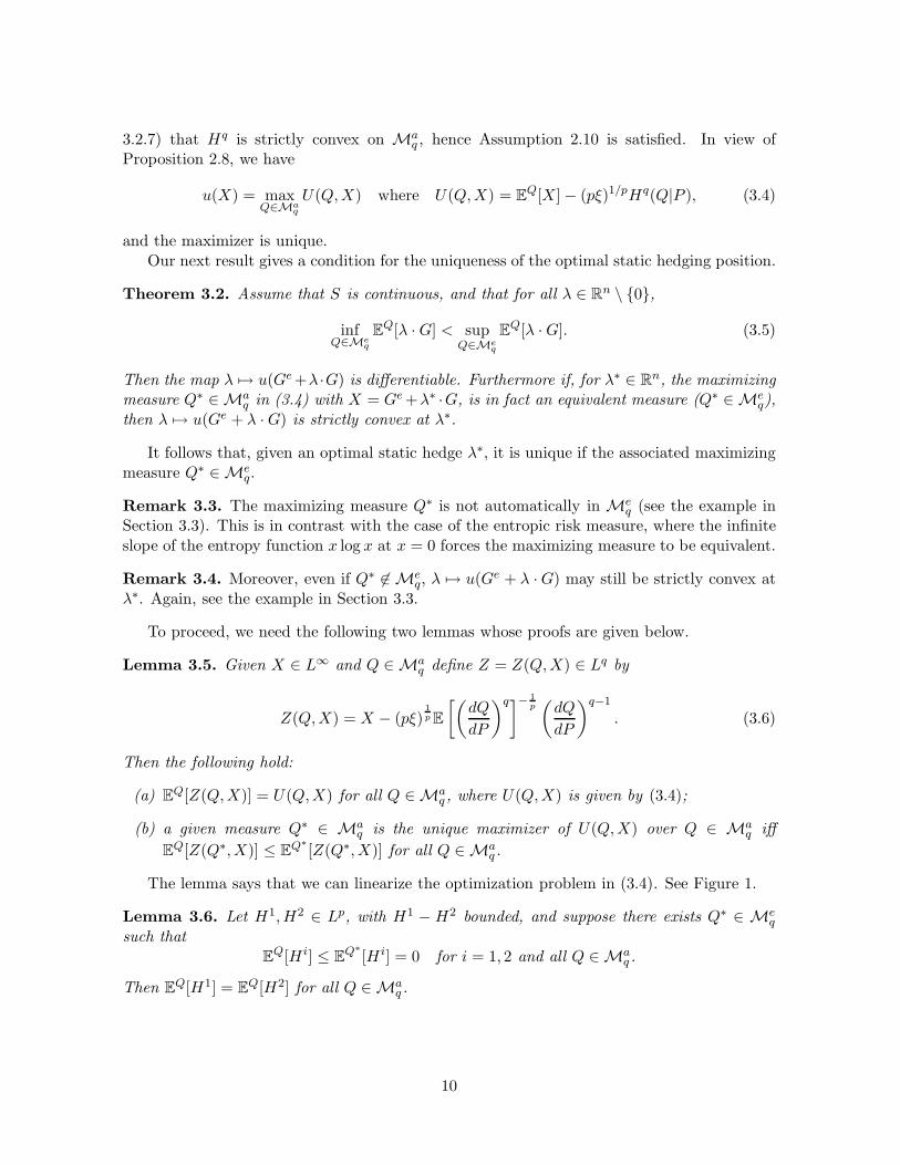
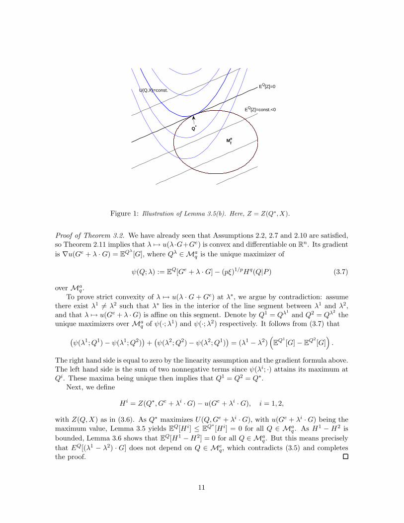
The lemma says that we can linearize the optimization problem in (3.4). See Figure 1.

Lemma 3.6. Let H1,H2 ∈ Lp, with H1 − H2 bounded, and suppose there exists Q∗ ∈ Meq

such thatE

Q[H i] ≤ EQ∗

[H i] = 0 for i = 1, 2 and all Q ∈ Maq .

Then EQ[H1] = E

Q[H2] for all Q ∈ Maq .

10

EQ[Z]=0

EQ[Z]=const.<0

U(Q,X)=const.

Mef

Q*

Figure 1: Illustration of Lemma 3.5(b). Here, Z = Z(Q∗, X).

Proof of Theorem 3.2. We have already seen that Assumptions 2.2, 2.7 and 2.10 are satisfied,so Theorem 2.11 implies that λ 7→ u(λ·G+Ge) is convex and differentiable on R

n. Its gradient

is ∇u(Ge + λ ·G) = EQλ

[G], where Qλ ∈ Maq is the unique maximizer of

ψ(Q;λ) := EQ[Ge + λ ·G] − (pξ)1/pHq(Q|P ) (3.7)

over Maq .

To prove strict convexity of λ 7→ u(λ · G +Ge) at λ∗, we argue by contradiction: assumethere exist λ1 6= λ2 such that λ∗ lies in the interior of the line segment between λ1 and λ2,and that λ 7→ u(Ge + λ ·G) is affine on this segment. Denote by Q1 = Qλ1

and Q2 = Qλ2

theunique maximizers over Ma

q of ψ(·;λ1) and ψ(·;λ2) respectively. It follows from (3.7) that

(

ψ(λ1;Q1) − ψ(λ1;Q2))

+(

ψ(λ2;Q2) − ψ(λ2;Q1))

= (λ1 − λ2)(

EQ1

[G] − EQ2

[G])

.

The right hand side is equal to zero by the linearity assumption and the gradient formula above.The left hand side is the sum of two nonnegative terms since ψ(λi; ·) attains its maximum atQi. These maxima being unique then implies that Q1 = Q2 = Q∗.

Next, we define

H i = Z(Q∗, Ge + λi ·G) − u(Ge + λi ·G), i = 1, 2,

with Z(Q,X) as in (3.6). As Q∗ maximizes U(Q,Ge + λi ·G), with u(Ge + λi ·G) being themaximum value, Lemma 3.5 yields E

Q[H i] ≤ EQ∗

[H i] = 0 for all Q ∈ Maq . As H1 − H2 is

bounded, Lemma 3.6 shows that EQ[H1 −H2] = 0 for all Q ∈ Ma

q . But this means precisely

that EQ[(λ1 − λ2) · G] does not depend on Q ∈ Meq, which contradicts (3.5) and completes

the proof.

11

3.2 Proofs of Lemma 3.5 and Lemma 3.6

We now prove the two lemmas.

Proof of Lemma 3.5. The proof of (a) is a simple computation. To prove (b) we fix Q∗, Q ∈Ma

q and set φ(t) = U((1 − t)Q∗ + tQ,X) for 0 ≤ t ≤ 1. Then φ is concave on [0, 1], henceadmits one-sided derivatives everywhere. A direct computation shows that

φ′(0+) = EQ[Z(Q∗,X)] −EQ∗

[Z(Q∗,X)].

On the one hand, if Q∗ is the maximizer of U(·,X), then φ′(0+) ≤ 0 for any choice of Q. Onthe other hand, if Q∗ is not the maximizer, then we may pick Q such that φ(1) > φ(0). Theconcavity of φ then gives φ′(0+) > 0.

Lemma 3.6 is taken from Theorem 1.2 in [9]. It is re-written here in a modified form:the theorem in [9] concerns attainable claims, but the argument works for “approximatelysuper- and sub-hedgeable claims”, which is what we need. We give the modified proof forcompleteness. First we need a definition and lemma, cf. [9, p.747].

Definition 3.7. We call a predictable process a simple p-admissible integrand for S if it is alinear combination of processes of the form

θ = f1]T1,T2],

where T1 and T2 are finite stopping times dominated by some Un, where (Un)∞n=1 is a localizingsequence for S; and f ∈ L∞(Ω,FT1

, P ). We define

Ksp =

∫ T

0θu dSu | θ simple p-admissible

⊂ Lp(P ).

Lemma 3.8.

H ∈ Ksp − Lp

+(P )Lp(P ) ⇐⇒ E

Q[H] ≤ 0, for all Q ∈ Maq ;

H ∈ Ksp + Lp

+(P )Lp(P ) ⇐⇒ E

Q[H] ≥ 0, for all Q ∈ Maq .

Proof. Follows from a simple modification of the proofs of (i) ⇐⇒ (iii′) in [9, Theorem 1.2].

Proof of Lemma 3.6. Adapting the approach in the proof of [9, Theorem 1.2], we proceed in

three steps, first to show that H i ∈ Ksp − Lp

+(P )Lp(P )

, then that H i ∈ Ksp

L1(Q∗), and finally

that H1 −H2 ∈ Ksp

Lp(P ). The first step follows from Lemma 3.8. Since Lp(P ) ⊂ L1(Q∗) (by

Holder’s inequality), we have that H i ∈ Ksp − L1

+(Q∗)L1(Q∗)

, and there exist two sequences(H i

n)∞n=1 ∈ Ksp , i = 1, 2 such that

limn→∞

EQ∗

(H i −H in)− = 0, i = 1, 2.

From the facts that elements of Ksp have Q∗-expectation zero, and that E

Q∗[H i] = 0, we

deducelim

n→∞E

Q∗|H i −H in| = 0, i = 1, 2,

12

in other words the H i are in the L1(Q∗) closure of Ksp . Then H := H1 − H2 is also in the

L1(Q∗) closure of Ksp, and is bounded by hypothesis.

For the last step, we may identify H with a uniformly integrable martingale (ht)t≥0 byletting ht = E

Q∗[H |Ft], and applying Corollary 2.5.2 in [30] to exhibit a predictable integrand

ϕ such that∫ T0 ϕu dSu = H. Note that

∫ t0 ϕu dSu = E

Q∗[H |Ft] is bounded in absolute

value by ||H||∞. Since we assumed that S is continuous, we can apply Lemma 2.3 in [9] to

find a sequence (ϕn)∞n=1 of ∞-admissible simple integrands such that∫ T0 ϕn

u dSu converges to∫ T0 ϕu dSu = H in Lp(P ). Therefore H is also in Ks

pLp(P )

. But then Lemma 3.8 implies that

EQ[H] = 0 for all Q ∈ Ma

q , and the conclusion of the lemma follows.

3.3 A Simple Example

We present a simple one-period quadrinomial tree example that demonstrates that even ifthe maximizing measure Q∗ in (3.4) with X = Ge + λ∗ · G is in Ma

q , but not in Meq, then

λ 7→ u(Ge +λ ·G) may still be strictly convex at λ∗. In other words, the condition in Theorem3.2 that the maximizing measure is not only absolutely continuous (with respect to P ) butalso equivalent, is sufficient, but not necessary for strict convexity.

The probability space has four elements: Ω = ω1, ω2, ω3, ω4 . The current stock price isS0 = 4, and at the end of the single period, ST (Ω) = 7, 5, 3, 1, with historical probabilities

P (ω1) =1

2, P (ω2) =

1

4, P (ω3) =

1

8, P (ω4) =

1

8.

The exotic option Ge and the single static hedging instrument G have payoffs

Ge(Ω) = −40,−20,−20,−40, G(Ω) = 3,−1, 1, 3.The absolutely continuous martingale measures Q ∈ Ma

q are parametrized by (q1, q2, q3, q4) ∈[0, 1]4, with the (probability and martingale) constraints

q1 + q2 + q3 + q4 = 1, 7q1 + 5q2 + 3q3 + q4 = 4.

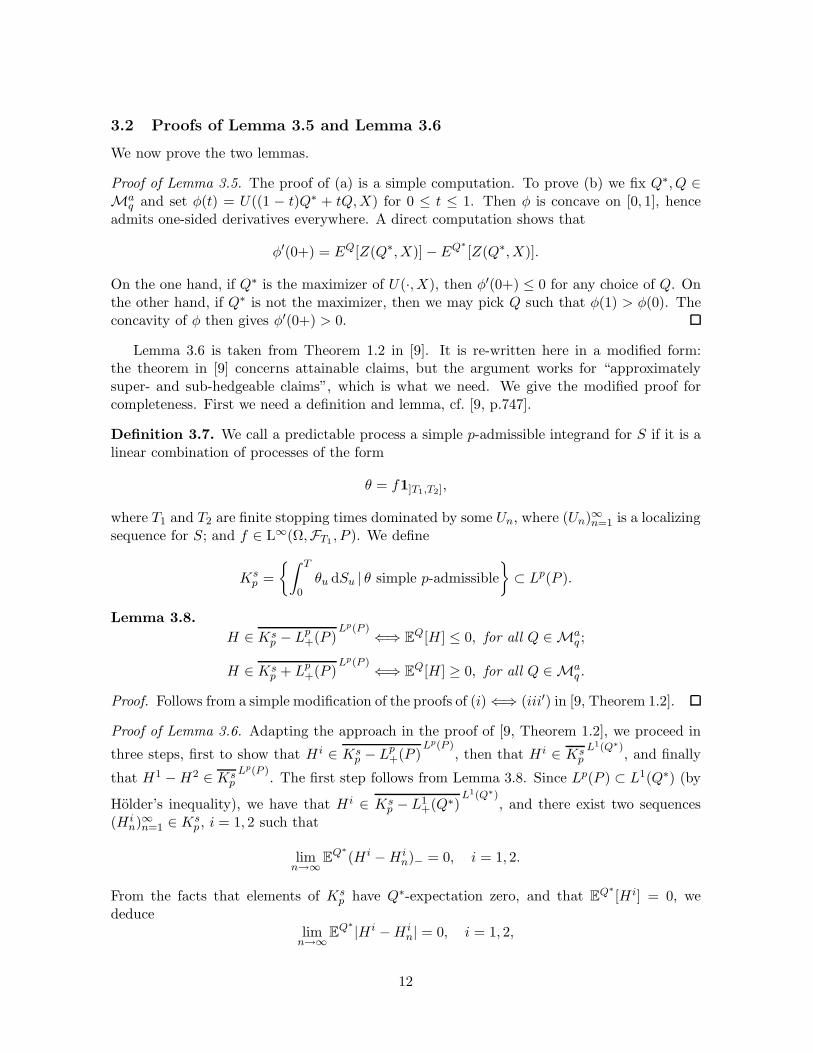
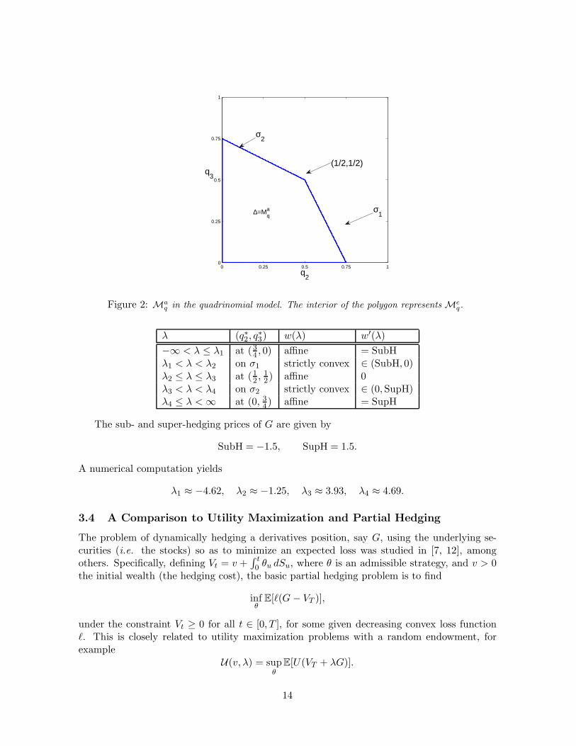
This is conveniently represented as (q2, q3) ∈ ∆, where ∆ is the convex subset of [0, 1]2 shownin Figure 2.

We choose p = q = 2 and the shortfall threshold level ξ such that the optimization problem(3.4) is

w(λ) := u(Ge + λG) = maxQ∈Ma

q

EQ[Ge + λG] −H2(Q | P ),

which, in the quadrinomial model, becomes of the form

w(λ) = max(q2,q3)∈∆

L(q2, q3) −√

Q(q2, q3),

for some affine function L, and quadratic function Q.It is straightforward, but tedious, to see that for any λ ∈ R, the optimizing measure is

always attained on the boundary of ∆, and so is absolutely continuous, but not equivalent.In particular, there exist finite λ1 < λ2 < λ3 < λ4 such that the optimizer (q∗2 , q

∗3) is either

on the edges σ1 and σ2 in Figure 2, or at the vertices (34 , 0), (1

2 ,12) or (0, 3

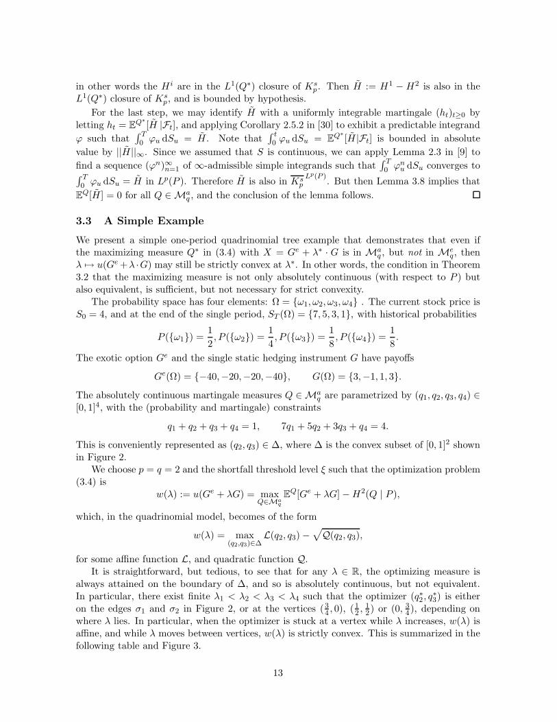
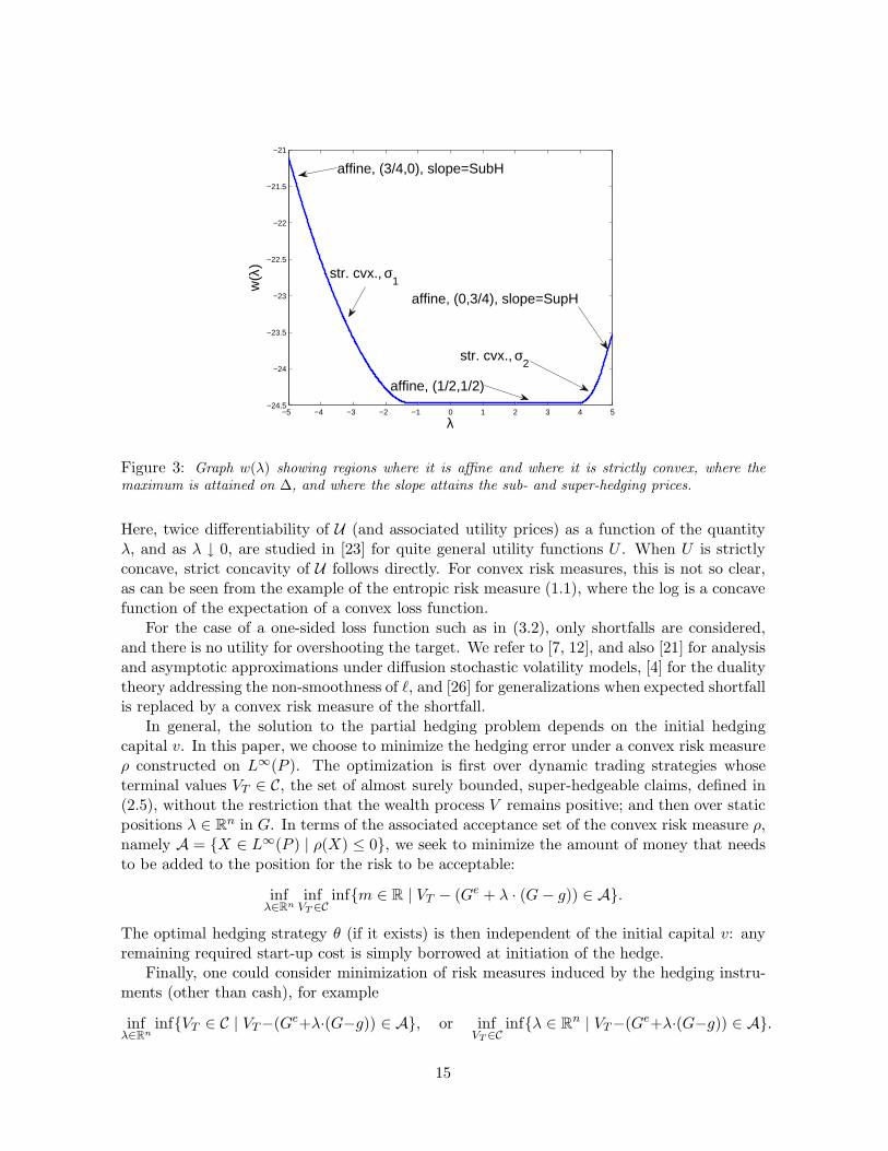
4), depending onwhere λ lies. In particular, when the optimizer is stuck at a vertex while λ increases, w(λ) isaffine, and while λ moves between vertices, w(λ) is strictly convex. This is summarized in thefollowing table and Figure 3.

13

0 0.25 0.5 0.75 10

0.25

0.5

0.75

1

q2

q3

∆=Mqa

σ2

(1/2,1/2)

σ1

Figure 2: Ma

qin the quadrinomial model. The interior of the polygon represents Me

q.

λ (q∗2, q∗3) w(λ) w′(λ)

−∞ < λ ≤ λ1 at (34 , 0) affine = SubH

λ1 < λ < λ2 on σ1 strictly convex ∈ (SubH, 0)λ2 ≤ λ ≤ λ3 at (1

2 ,12) affine 0

λ3 < λ < λ4 on σ2 strictly convex ∈ (0,SupH)λ4 ≤ λ <∞ at (0, 3

4) affine = SupH

The sub- and super-hedging prices of G are given by

SubH = −1.5, SupH = 1.5.

A numerical computation yields

λ1 ≈ −4.62, λ2 ≈ −1.25, λ3 ≈ 3.93, λ4 ≈ 4.69.

3.4 A Comparison to Utility Maximization and Partial Hedging

The problem of dynamically hedging a derivatives position, say G, using the underlying se-curities (i.e. the stocks) so as to minimize an expected loss was studied in [7, 12], amongothers. Specifically, defining Vt = v +

∫ t0 θu dSu, where θ is an admissible strategy, and v > 0

the initial wealth (the hedging cost), the basic partial hedging problem is to find

infθ

E[ℓ(G− VT )],

under the constraint Vt ≥ 0 for all t ∈ [0, T ], for some given decreasing convex loss functionℓ. This is closely related to utility maximization problems with a random endowment, forexample

U(v, λ) = supθ

E[U(VT + λG)].

14

−5 −4 −3 −2 −1 0 1 2 3 4 5−24.5

−24

−23.5

−23

−22.5

−22

−21.5

−21

λ

w(λ

)

str. cvx., σ2

affine, (0,3/4), slope=SupH

affine, (1/2,1/2)

affine, (3/4,0), slope=SubH

str. cvx., σ1

Figure 3: Graph w(λ) showing regions where it is affine and where it is strictly convex, where themaximum is attained on ∆, and where the slope attains the sub- and super-hedging prices.

Here, twice differentiability of U (and associated utility prices) as a function of the quantityλ, and as λ ↓ 0, are studied in [23] for quite general utility functions U . When U is strictlyconcave, strict concavity of U follows directly. For convex risk measures, this is not so clear,as can be seen from the example of the entropic risk measure (1.1), where the log is a concavefunction of the expectation of a convex loss function.

For the case of a one-sided loss function such as in (3.2), only shortfalls are considered,and there is no utility for overshooting the target. We refer to [7, 12], and also [21] for analysisand asymptotic approximations under diffusion stochastic volatility models, [4] for the dualitytheory addressing the non-smoothness of ℓ, and [26] for generalizations when expected shortfallis replaced by a convex risk measure of the shortfall.

In general, the solution to the partial hedging problem depends on the initial hedgingcapital v. In this paper, we choose to minimize the hedging error under a convex risk measureρ constructed on L∞(P ). The optimization is first over dynamic trading strategies whoseterminal values VT ∈ C, the set of almost surely bounded, super-hedgeable claims, defined in(2.5), without the restriction that the wealth process V remains positive; and then over staticpositions λ ∈ R

n in G. In terms of the associated acceptance set of the convex risk measure ρ,namely A = X ∈ L∞(P ) | ρ(X) ≤ 0, we seek to minimize the amount of money that needsto be added to the position for the risk to be acceptable:

infλ∈Rn

infVT ∈C

infm ∈ R | VT − (Ge + λ · (G− g)) ∈ A.

The optimal hedging strategy θ (if it exists) is then independent of the initial capital v: anyremaining required start-up cost is simply borrowed at initiation of the hedge.

Finally, one could consider minimization of risk measures induced by the hedging instru-ments (other than cash), for example

infλ∈Rn

infVT ∈ C | VT−(Ge+λ·(G−g)) ∈ A, or infVT ∈C

infλ ∈ Rn | VT−(Ge+λ·(G−g)) ∈ A.

15

The first is the minimization of a C-valued risk measure over static hedges, the latter theminimization of a vector valued risk measure over dynamic hedges. Formulation of the problemof course requires defining the notion of infimum for set-valued risk measures. We refer to [16]for work in this direction.

4 Varying the shortfall threshold

With a view towards numerical computations (Section 5), we study the properties of u as afunction of the threshold level ξ > 0, which we introduce as an argument in the notation,denoting U and u in (3.4) as U(ξ,Q,X) and u(ξ,X), respectively.

As 1 < q <∞, U is strictly convex in ξ. Let us introduce its Fenchel-Legendre transform:

U(z,Q,X) = infξ>0

(U(ξ,Q,X) + ξz), z ≥ 0, (4.1)

= EQ[X] − 1

qz1−q

E

[(

dQ

dP

)q]

,

and the conjugate optimization problem

u(z,X) = supQ∈Ma

q

U(z,Q,X). (4.2)

Note that u(z,−X) is another market modified convex risk measure with penalty function1qz

1−qE

[(

dQdP

)q]

, which is finite and strictly convex on Maq . The important difference with

the dual representation (3.4) of u is that the “outside power” 1/q is missing compared with(3.3), and the objective function U is therefore an expectation of a function of the Radon-Nikodym derivative dQ/dP . This is exploited when we use dynamic programming for anumerical computation in Section 5.

Theorem 4.1. For X ∈ L∞, we have

u(ξ,X) = supz>0

(u(z,X) − ξz) , (4.3)

andu(z,X) = inf

ξ>0(u(ξ,X) + ξz) . (4.4)

We will make use of the following analog of Lemma 3.5 part (b). The proof, being almostidentical, is omitted.

Lemma 4.2. Given z > 0, X ∈ L∞ and Q ∈ Maq define W = W (z,Q,X) ∈ Lq by

W (z,Q,X) = X − z1−q

(

dQ

dP

)q−1

. (4.5)

Then a given measure Q∗ ∈ Maq is the unique maximizer of U(z,Q,X) over Q ∈ Ma

q iff

EQ[W (z,Q∗,X)] ≤ E

Q∗[W (z,Q∗,X)] for all Q ∈ Ma

q .

16

Proof of Theorem 4.1. The functions U(ξ,Q,X) and U(z,Q,X) being conjugate, we have

U(ξ,Q,X) = supz>0

(

U(z,Q,X) − ξz)

for Q ∈ Maq .

Taking supremum over Q in both sides, and changing the order of maximization problems onthe right hand side, we arrive at (4.3).

To prove (4.4) we fix z and let Q∗ ∈ Maq be (uniquely) defined by u(z,X) = U(z,Q∗,X).

By Lemma 4.2, we have EQ[W (z,Q∗,X)] ≤ EQ∗[W (z,Q∗,X)] for all Q ∈ Ma

q .

Next, we set ξ∗ = p−1z−qE[(dQ∗

dP )q]. A straightforward calculation shows thatW (z,Q∗,X) =Z(ξ∗, Q∗,X) where the right hand side is defined as in Lemma 3.5, using this same measureQ∗. Applying Lemma 4.2, we find that

EQ∗

[Z(ξ∗, Q∗,X)] = EQ∗

[W (z,Q∗,X)] ≥ EQ[W (z,Q∗,X)] = E

Q[Z(ξ∗, Q∗,X)],

for all Q ∈ Maq . Lemma 3.5 part (b) then implies that Q∗ maximizes U(ξ∗, Q,X), and so

we have u(ξ∗,X) = U(ξ∗, Q∗,X). A further direct computation reveals that U(z,Q∗,X) =U(ξ∗, Q∗,X) + ξ∗z, which yields

u(z,X) = U(z,Q∗,X) = U(ξ∗, Q∗,X) + ξ∗z = u(ξ∗,X) + ξ∗z ≥ infξ>0

(u(ξ,X) + ξz).

But (4.3) implies u(x,X) ≤ infξ>0(u(ξ,X) + ξz), and hence (4.4) holds.

5 Computation of Shortfall Risk in the Nontraded Asset Model

In this section, we address computation of the optimal hedge within a dynamic Brownianmotion based financial model. Our goal is to provide a comparison in a case where theentropic risk measure (or, equivalently, exponential utility) has been enormously successful,namely the problem of hedging (or indifference pricing) of an option on a non-traded asset,using a correlated tradeable asset. In the canonical set-up, the price processes of the tradedasset S and the non-traded asset Y are described by the stochastic differential equations

dSt = µ(Yt)St dt+ σ(Yt)St dW 1t , S0 = S, (5.1)

dYt = b(Yt) dt+ a(Yt)(ν dW 1t + ν ′ dW 2

t ), Y0 = y. (5.2)

Here W 1 and W 2 are independent standard Brownian motions on our probability space(Ω,F ,F, P ), and F = (Ft)0≤t≤T is the standard filtration generated by them. The constantν ∈ (−1, 1) is a correlation coefficient, and ν ′ =

√1 − ν2. We assume sufficient regularity on

the coefficients of the SDEs to guarantee existence of a unique strong solution. Specifically, weassume that a and σ are bounded above and below away from zero, and smooth with boundedderivatives. We also assume that µ and b are smooth with bounded derivatives. The objectof interest is a European derivative contract written on Y .

5.1 Dynamic Programming Equation

For our hedging problem, the option payoffs that we need to work with will be path dependentin general, but to ease the representation, in this section we will assume that Ge+λG = h(YT ),

17

that is, European. The extension to path dependent payoffs would introduce additional bound-ary conditions, and/or extra dimensions in the resulting Hamilton-Jacobi-Bellman (HJB)equations we will use for analysis of the optimization problems.

One approach would be to deal with the primal problem (2.9). In this case, to apply dy-namic programming techniques, we introduce the wealth process Vt corresponding to holding,at time t, πt dollars in the traded asset S. We will assume throughout that the interest rateis zero, and so the wealth process evolves according to

dVt = µ(Yt)πt dt+ σ(Yt)πt dW 1t , V0 = v. (5.3)

The value function of the dynamic hedging problem is then defined as

H(t, v, y) = infπ

E [ℓ((h(YT ) − VT ))|Vt = v, Yt = y] , (5.4)

and the shortfall risk w at level ξ is found (at time zero) by solving

H(0, v + w, y) = ξ.

It might be natural here to pass to the HJB equation for H, but for the loss function (3.2),we know that H ≡ 0 for v large enough, particularly v ≥ vsup, the superhedging price (amongadmissible strategies that trade only S) of the claim h. Therefore, H may not have sufficientsmoothness for the HJB equation to apply for all v ∈ R, and we pass to the study of the dualproblem (4.2).

From Girsanov’s theorem, the set of equivalent local martingale measures is characterizedin the model (5.1)-(5.2) by

dQγ

dP= exp

(

−∫ T

0

µ(Yt)

σ(Yt)dW 1

t −∫ T

0γt dW 2

t − 1

2

∫ T

0

(

µ2(Yt)

σ2(Yt)+ γ2

t

)

dt

)

,

for some adapted process γ with∫ T0 γ2

t dt < ∞ a.s. We denote by N the space of adapted

processes γ that satisfy the Novikov condition: E[exp(12

∫ T0 γ2

t dt)] < ∞. For γ ∈ N , Qγ

is then an equivalent martingale measure, and by Jensen’s inequality, the Novikov conditionimplies E[

∫ T0 γ2

t dt] <∞.

Remark 5.1. The q-distance of Qγ with respect to P is

Hq(Qγ | P ) = E

[

exp

(

−1

2q

∫ T

0

(

µ2(Yt)

σ2(Yt)+ γ2

t

)

dt− q

∫ T

0

µ(Yt)

σ(Yt)dW 1

t − q

∫ T

0γt dW 2

t

)]1/q

.

The choice γ ≡ 0 gives the well-known minimal martingale measure Q0. By the assumptionson the coefficients, Hq(Q0 | P ) <∞, and so Me

q is non-empty, and Assumption 2.7 is satisfied.

For γ ∈ N , we define

W γ,1t = W 1

t +

∫ t

0

µ(Ys)

σ(Ys)ds, W γ,2

t = W 2t +

∫ t

0γs ds

and the process (Zt) by

dZt = Zt

(

µ(Yt)

σ(Yt)dW γ,1

t + γtdWγ,2t

)

, Z0 = z.

18

By Girsanov’s theorem, W γ,1 and W γ,2 are Qγ-Brownian motions. Moreover, ZT = z dPdQγ and

(Zt) is a Qγ-martingale.We are interested in computing u(z, h(YT )) of equation (4.2). A priori we have to optimize

over all absolutely continuous local martingale measures of finite q-distance, that is, Q ∈ Maq .

The supremum does not change (but may no longer be attained) if we optimize over onlyequivalent local martingale measures, that is, Q ∈ Me

q.

Assumption 5.2. Assume that we only need to optimize over measures of the form Qγ , whereγ satisfies the Novikov condition:

u(z, h(YT )) = supγ∈N

(

EQγ

[h(YT )] − 1

qz1−q

E

[(

dQγ

dP

)q])

. (5.5)

Re-writing (5.5) as

u(z, h(YT )) = supγ∈N

(

EQγ

[h(YT )] − 1

qz1−q

EQγ

[

(

dQγ

dP

)q−1])

,

leads us to consider the value function

u(t, y, z) = supγ∈N

EQγ

[

h(YT ) − 1

qZ1−q

T | Yt = y, Zt = z

]

, (5.6)

which we have also labeled u in a slight abuse of notation.

Proposition 5.3. Suppose i) Assumption 5.2 holds; ii) the value function u(t, y, z) is con-tinuously differentiable in t and twice continuously differentiable in y and z, and is strictlyconcave in z; and iii) that γ∗t defined by

γ∗t = −√

1 − ν2 a(Yt)(Zt uzy(t, Yt, Zt) − uy(t, Yt, Zt))

Z2t uzz(t, Yt, Zt)

satisfies Novikov’s condition. Then u(t, y, z) satisfies the HJB equation

ut + Lyu+νµ(y)a(y)

σ(y)(zuzy − uy) +

µ2(y)

2σ2(y)z2uzz −

1

2a2(y)(1 − ν2)

(zuzy − uy)2

z2uzz= 0, (5.7)

with the terminal condition

u(T, y, z) = h(y) − 1

qz1−q, (5.8)

where

Ly =1

2a2(y)

∂2

∂y2+ b(y)

∂

∂y. (5.9)

The optimum in (5.6) is attained by (γ∗t ).

Proof. Clearly for γ ∈ N ,dQγ

dP= zZ−1

T ,

and, under Qγ ,

dYt =

(

b(Yt) − νµ(Yt)

σ(Yt)a(Yt) − ν ′a(Yt)γt

)

dt+ a(Yt)(ν dW γ,1t + ν ′dW γ,2

t ), Y0 = y.

Given the strong regularity assumptions, the results follow from standard verification argu-ments [11].

19

An alternative derivation at the level of value functions, obtained from the HJB equationfor H in (5.4) associated with the primal problem, is given in Appendix A.

Remark 5.4. In the case of the exponential loss function ℓ(x) = eγx, the analysis and theresulting PDEs are the same, only the terminal conditions change. In particular, (5.8) becomesu(T, y, z) = h(y) + γ−1(1 + log(γz)). Then the solution to (5.7) is additively separable in yand z, and is given by

u(t, y, z) = K(t, y) + L(z), (5.10)

where L(z) = γ−1 log(γz), and

K(t, y) =1

γ+

1

(1 − ν2)log E

Q0

[

exp

(

−∫ T

t

µ2(Ys)(1 − ν2)

2σ2(Ys)ds+ (1 − ν2)h(YT )

)

| Yt = y

]

.

We refer to [24]. This simplification is particular to the exponential loss function, and ofcourse can be exploited in the dual problem itself without passing to the conjugate.

In general, the PDE problem (5.7) is not analytically tractable, but for a very specialcase as when the terminal condition comes from the exponential loss function, as discussedin Remark 5.4. For the terminal condition (5.8) coming from our power loss function, thesolution is not separable as (5.10), even if L is allowed to depend on t as well. However, in thecase of no claim (h ≡ 0), the dual problem is to find the q-optimal measure that minimizes

E

[(

dQγ

dP

)q]

.

This problem is considered in some generality in [15], and for stochastic volatility models in[17, 25]. Similarly, conditions for verifying the optimality of a candidate measure which involveonly that measure are available in the case of the entropic risk measure [15, Proposition 3.2],and in the problem of finding the q-optimal measure when there is no claim [15, Proposition4.2], but we are not aware of a similar result in the latter case when there is a claim, andverification remains an open problem.

5.2 Numerical Solution

To illustrate the market-adjusted shortfall risk measure of a derivatives position, we present anumerical solution of the PDE for the conjugate of the dual problem, which is then Legendre-transformed to return the risk measure. Specifically, we suppose that the claim on Y is a putoption with strike K:

h(YT ) = (K − YT )+,

where Y is a geometric Brownian motion:

dYt = bYt dt+ aYt (ν dW 1t + ν ′ dW 2

t ), (5.11)

and we want to compute the risk

u = infπρ (h(YT ) − VT ) ,

20

where ρ is the shortfall risk measure with quadratic power loss function and thereshold ξ,defined in (3.1)-(3.2), with p = 2, and VT is the terminal value of the hedging portfolio,defined in (5.3).

We do not tackle here the problem of hedging exotic options with the underlying and othervanilla options. In the case of the exponential loss function, numerical solutions for the fullstatic-dynamic hedging of barrier options are given in [20], but we leave for a future workextension of this to the power loss shortfall case.

Since the initial wealth level v merely reduces the risk by subtraction, we take v = 0without loss of generality. Then, by Theorem 4.1, given the solution u(0, Y0, z), the risk underthis measure of the short put position, mitigated by trading optimally in the correlated assetS, is given by

u = supz>0

(u(0, Y0, z) − ξz) . (5.12)

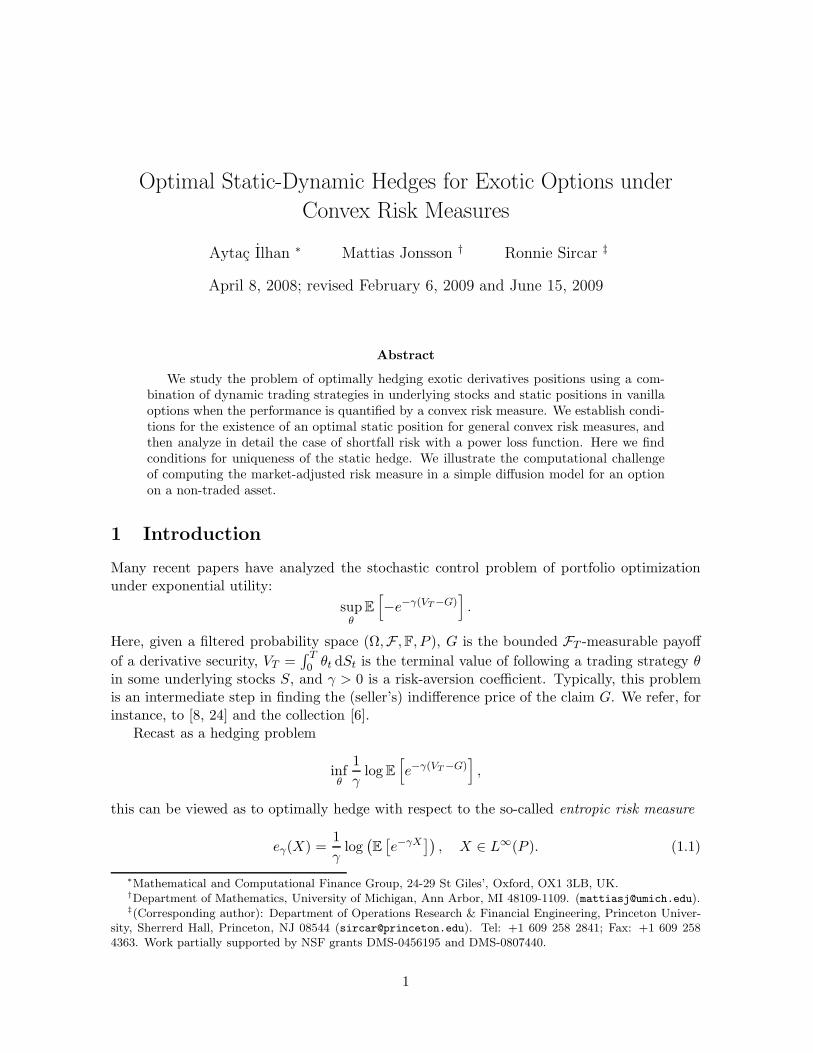
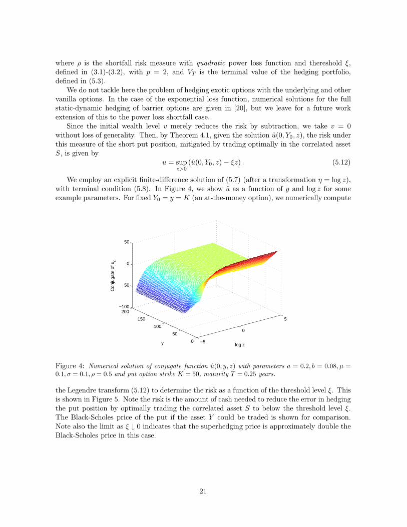
We employ an explicit finite-difference solution of (5.7) (after a transformation η = log z),with terminal condition (5.8). In Figure 4, we show u as a function of y and log z for someexample parameters. For fixed Y0 = y = K (an at-the-money option), we numerically compute

−5

0

5

0

50

100

150

200−100

−50

0

50

log zy

Con

juga

te o

f u0

Figure 4: Numerical solution of conjugate function u(0, y, z) with parameters a = 0.2, b = 0.08, µ =0.1, σ = 0.1, ρ = 0.5 and put option strike K = 50, maturity T = 0.25 years.

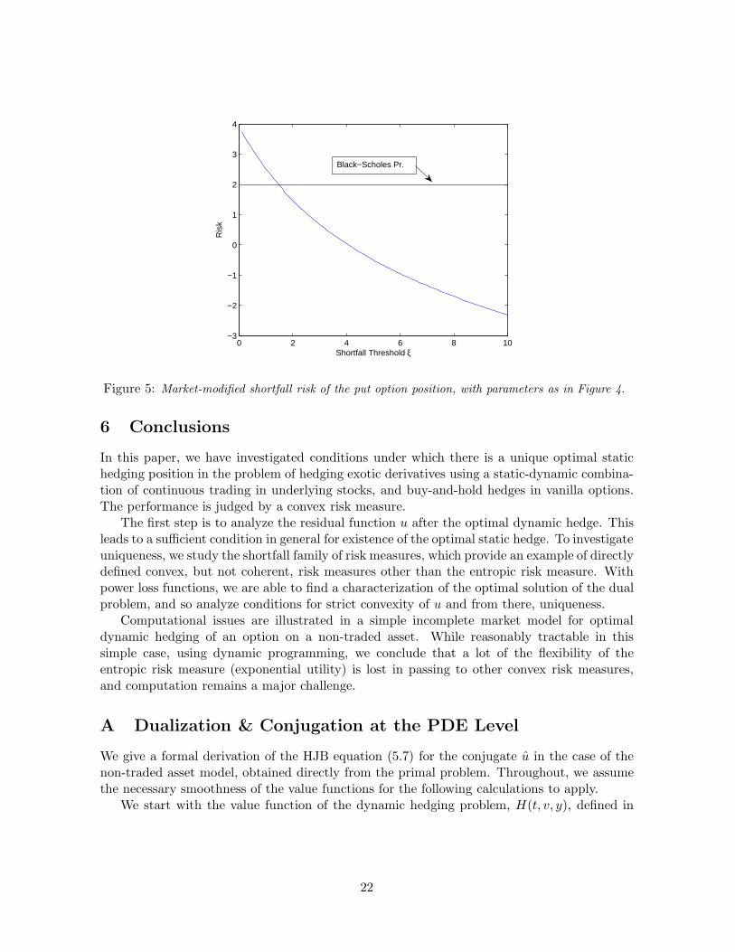
the Legendre transform (5.12) to determine the risk as a function of the threshold level ξ. Thisis shown in Figure 5. Note the risk is the amount of cash needed to reduce the error in hedgingthe put position by optimally trading the correlated asset S to below the threshold level ξ.The Black-Scholes price of the put if the asset Y could be traded is shown for comparison.Note also the limit as ξ ↓ 0 indicates that the superhedging price is approximately double theBlack-Scholes price in this case.

21

0 2 4 6 8 10−3

−2

−1

0

1

2

3

4

Shortfall Threshold ξ

Ris

k

Black−Scholes Pr.

Figure 5: Market-modified shortfall risk of the put option position, with parameters as in Figure 4.

6 Conclusions

In this paper, we have investigated conditions under which there is a unique optimal statichedging position in the problem of hedging exotic derivatives using a static-dynamic combina-tion of continuous trading in underlying stocks, and buy-and-hold hedges in vanilla options.The performance is judged by a convex risk measure.

The first step is to analyze the residual function u after the optimal dynamic hedge. Thisleads to a sufficient condition in general for existence of the optimal static hedge. To investigateuniqueness, we study the shortfall family of risk measures, which provide an example of directlydefined convex, but not coherent, risk measures other than the entropic risk measure. Withpower loss functions, we are able to find a characterization of the optimal solution of the dualproblem, and so analyze conditions for strict convexity of u and from there, uniqueness.

Computational issues are illustrated in a simple incomplete market model for optimaldynamic hedging of an option on a non-traded asset. While reasonably tractable in thissimple case, using dynamic programming, we conclude that a lot of the flexibility of theentropic risk measure (exponential utility) is lost in passing to other convex risk measures,and computation remains a major challenge.

A Dualization & Conjugation at the PDE Level

We give a formal derivation of the HJB equation (5.7) for the conjugate u in the case of thenon-traded asset model, obtained directly from the primal problem. Throughout, we assumethe necessary smoothness of the value functions for the following calculations to apply.

We start with the value function of the dynamic hedging problem, H(t, v, y), defined in

22

(5.4). Its associated HJB equation is

Ht + LyH + infπ

(

1

2π2σ2(y)Hvv + π(µ(y)Hv + ρσ(y)a(y)Hvy)

)

= 0 (A.1)

with

H(T, v, y) =1

p

(

(h(y) − v)+)p,

where Ly, defined in (5.9), is the infinitesimal generator of Y . Evaluating the internal minimumsupposing that Hvv > 0 in t < T gives

Ht + LyH − (µ(y)Hv + ρσ(y)a(y)Hvy)2

2σ2(y)Hvv= 0.

For v less than the superhedging price of the claim, we need to find the “inverse” of H,namely the solution w of

H(t, v + w(t, v, y, ξ), y) = ξ.

Then it follows easily that w = −v + u(t, y, ξ), for some function u, which is in fact the totalcapital needed to reduce the expected shortfall to level ξ. (The additional capital w is foundby simply reducing u by the initial capital v). By successive differentiation of the identityH(t, u(t, y, ξ), y) = ξ, we obtain the following PDE problem for u:

ut +1

2a2(y)

(

uyy − 2uξyuy

uξ+uξξu

2y

u2ξ

)

+ b(y)uy

−(µ(y)uξ − ρσ(y)a(y)uyξ + ρa(y)σ(y)

uyuξξ

uξ)2

2σ2(y)uξξ= 0

withu(T, y, ξ) = h(y) − (pξ)1/p.

Note that we need to treat ξ as a variable in order to have a self-contained equation for u.Next, we introduce the Legendre transform of u

u(t, y, z) = infξ>0

(u(t, y, ξ) + ξz) ,

and the optimizer χ(t, y, z) that solves

uξ(t, y, χ) = −z.

Then, successively differentiating and manipulating this expression, we substitute partialderivatives of u in terms of u and obtain

ut + Lyu+ρµa(y)

σ(zuzy − uy) +

µ2

2σ2z2uzz −

1

2a2(y)(1 − ρ2)

(zuzy − uy)2

z2uzz= 0,

which is exactly (5.7).

23

References

[1] P. Artzner, F. Delbaen, J. M. Eber, and D. Heath. Coherent measures of risk. Math.Finance, 9:203–228, 1999.

[2] P. Barrieu and N. El Karoui. Inf-convolution of risk measures and optimal risk transfer.Finance and Stochastics, 9(2):269–298, 2005.

[3] P. Barrieu and N. El Karoui. Pricing, hedging and optimally designing derivatives viaminimization of risk measures. In R. Carmona, editor, Indifference Pricing. PrincetonUniversity Press, 2008.

[4] B. Bouchard, N. Touzi, and A. Zeghal. Dual formulation of the utility maximizationproblem: The case of nonsmooth utility. The Annals of Applied Probability, 14(2):678–717, 2004.

[5] J. Bowie and P. Carr. Static simplicity. Risk, 7:45–49, 1994.

[6] R. Carmona, editor. Indifference Pricing. Princeton University Press, 2008.

[7] J. Cvitanic and I. Karatzas. On dynamic measures of risk. Finance and Stochastics, 3(4),1999.

[8] F. Delbaen, P. Grandits, T. Rheinlander, D. Samperi, M. Schweizer, and C. Stricker.Exponential hedging and entropic penalties. Mathematical Finance, 12(2):99–123, 2002.

[9] F. Delbaen and W. Schachermayer. Attainable claims with p’th moments. Ann. Inst. H.Poincare Probab. Statist., 32(6):743–763, 1996.

[10] D. Filipovic and G. Svindland. The canonical model space for law-invariant convex riskmeasures is L1. Mathematical Finance, 2009. To appear.

[11] W. Fleming and H.M. Soner. Controlled Markov Processes and Viscosity Solutions.Springer, 2nd edition, 2005.

[12] H. Follmer and P. Leukert. Efficient hedging: Cost versus shortfall risk. Finance andStochastics, 4(2):117–146, 2000.

[13] H. Follmer and A. Schied. Stochastic Finance: An Introduction in Discrete Time. DeGruyter Studies in Mathematics. Walter de Gruyter, 2nd edition, 2004.

[14] Avner Friedman. Foundations of Modern Analysis. Dover Publications Inc, 1970.

[15] P. Grandits and T. Rheinlander. On the minimal entropy martingale measure. TheAnnals of Probability, 30(3):1003–1038, 2002.

[16] A. Hamel, F. Heyde, and M. Hohne. Set-valued measures of risk. Technical report,Princeton University, 2007.

[17] D. Hobson. Stochastic volatility models, correlation and the q-optimal measure. Mathe-matical Finance, 14(4):537–556, 2004.

24

[18] A. Ilhan, M. Jonsson, and R. Sircar. Optimal investment with derivative securities.Finance & Stochastics, 9:585–595, 2005.

[19] A. Ilhan, M. Jonsson, and R. Sircar. Portfolio optimization with derivatives and indif-ference pricing. In R. Carmona, editor, Indifference Pricing. Princeton University Press,2008.

[20] A. Ilhan and R. Sircar. Optimal static-dynamic hedges for barrier options. MathematicalFinance, 16:359–385, 2006.

[21] M. Jonsson and R. Sircar. Partial hedging in a stochastic volatility environment. Math-ematical Finance, 12(4):375–409, October 2002.

[22] S. Kloppel and M. Schweizer. Dynamic utility indifference valuation via convex measures.Technical report, NCCR FINRISK, ETH Zurich, 2005. Shorter version in MathematicalFinance vol. 17, pages 599-627, 2007.

[23] D. Kramkov and M. Sirbu. Sensitivity analysis of utility based prices and risk-tolerancewealth processes. Annals of Applied Probability, 16(4):2140–2194, 2006.

[24] M. Musiela and T. Zariphopoulou. An example of indifference prices under exponentialpreferences. Finance and Stochastics, 8(2):229–239, 2004.

[25] T. Rheinlander. An entropy approach to the Stein and Stein model with correlation.Finance and Stochastics, 9(3):399–413, 2005.

[26] B. Rudloff. Convex hedging in incomplete markets. Applied Mathematical Finance,14(5):437 – 452, 2007.

[27] W. Schachermayer. Introduction to the mathematics of financial markets. In PierreBernard, editor, Lectures on Probability Theory and Statistics, Saint-Fleur summer school2000, number 1816 in Lecture Notes in Mathematics, pages 111–177. Springer Verlag,2003.

[28] A. Toussaint. Hedging under L2 convex risk measures. Technical report, PrincetonUniversity, 2006.

[29] A. Toussaint and R. Sircar. A framework for dynamic hedging under convex risk measures.In R. Dalang, M. Dozzi, and F. Russo, editors, Proceedings of the Fifth Seminar onStochastic Analysis, Random Fields and Applications, Progress in Probability. BirkhauserVerlag, 2008. To appear.

[30] M. Yor. Sous-espaces denses dans L1 ou H1 et representation des martingales. InSeminaire de Probabilites XII, number 649 in Lecture Notes in Mathematics, pages 205–309. Springer, 1978.

25