Optimal control of an elastically connected rectangular plate–membrane system

Journal of Computational and Applied Mathematics 180 (2005) 345–363

www.elsevier.com/locate/cam

Optimal control of an elastically connected rectangularplate–membrane systemIsmail Kucuk∗, Ibrahim Sadek

Department of Mathematics and Statistics, American University of Sharjah, P.O. Box 26666, Sharjah, United Arab Emirates

Received 30 May 2004; received in revised form 1 November 2004

Abstract

The optimal control of an elastically connected rectangular plate–membrane system by point-wise actuators isconsidered. Problems of the type are of significant practical interest in most real mechanical structures widely usedin aeronautical, civil, naval, and mechanical engineering. An index of performance is formulated, which consistsof a modified energy functional of the two coupled structure at a specified time and penalty functions involving thepoint control actuators. Necessary conditions of optimality are derived in the form of independent integral equationswhich lead to explicit expressions for the point-wise actuators. The results are applied to a specific problem, andnumerical results are given that reveal the effectiveness of the proposed control mechanism.© 2004 Elsevier B.V. All rights reserved.

Keywords:Optimal control; Plate; Membrane; Integral equations; Elasticity

1. Introduction

Mechanical structures can be modelled as one-dimensional simple continuous systems such as a stringand beam or two-dimensional simple continuous systems such as a membrane and plate. The simplemodels are used in complex continuous systems such as an elastically connected double-solid systemthat consists of two elastic solids bounded continuously through a Winkler elastic layer. The vibrationanalysis of complex continuous systems is one of the tools used in civil and mechanical engineeringfor theoretical and practical applications of the problems raising in engineering[10,14,15]. Complex

∗ Corresponding author. Tel.: +97165152921; fax: +97165152950.E-mail address:[email protected](I. Kucuk).

0377-0427/$ - see front matter © 2004 Elsevier B.V. All rights reserved.doi:10.1016/j.cam.2004.11.005

http://www.elsevier.com/locate/cam

mailto:[email protected]

346 I. Kucuk, I. Sadek / Journal of Computational and Applied Mathematics 180 (2005) 345–363

continuous systems of special types are studied in depth for transverse vibration theory[10]. One of thecentral problems in design of these structures is vibration suppression. Vibration control is an importantproblem and many methods for both active and passive vibration absorption have been developed. Thispaper dealswith developing amethod to achieve an optimal control of an elastically connected rectangularplate–membrane system by applying a finite number of actuators along the two structures. The controlvibration analysis of this continuous system has theoretical and practical importance, and has a wideapplication in civil and mechanical engineering. The basic control problem is to minimize a performancefunction in a given period of time. The problem is then converted to that of optimal control of lumped-parameter systems by using the eigenfunction expansion of the state functions. Necessary conditionsof optimality which the control actuator must satisfy are derived in the form of integral equations usingvariational approach. Since the system of the integral equations is degenerate, the optimal control actuatorcan be found explicitly by solving a system of linear algebraic equations.The proposed approach is illustrated by a numerical example inwhich the two discrete control actuators

are applied to an elastically connected rectangular plate–membrane system.Thebehavior of the controlledand uncontrolled connected structure is numerically studied and the effectiveness of the proposed controlis illustrated for various parameters. Numerical results indicate that the dynamical response of the mixedsystem can be reduced substantially in a given period of time. This can be achieved by selecting a suitablevalue of the membrane tension and applying an actuator in the domain of the plate. Nonetheless, ifactuators are applied to both membrane and plate simultaneously, the structure becomes uncontrollabledue to the excessive vibrations.The problem considered in this paper is motivated due to the problems in[12,13]. In these papers, the

control vibration of flexible structures that consist of two Euler–Bernoulli beams coupled in parallel bymeans of the application of a finite number of actuators is investigated. Maximum principles are derivedfor optimal point-wise or boundary controls of such one-dimensional coupled structures undergoingtransverse vibrations. It is shown that the same system is uniformly exponentially stable by an appropriateapplication of either distributed or boundary control in[9]. On the other hand, there has been a workon the point-wise distributed and boundary control of distributed-parameter systems represented byNserially connected flexible structures that are coupled through boundary conditions[15,14]. Maximumprinciples are established for such a system ofN partial differential equations of second order in timeparameter and fourth order in space.There has been made a considerable number of publications on controllability and stability of serially

connected vibrating structures in the literature. In particular, the controllability and stability of a system ofcoupledstringswithnonconstantwavespeeds inwhichcontrol parametersareappliedat thecoupledpointsare studied in[6]. It is shown that the system is approximately controllable if and only if related systems ofuncoupled strings do not share a common eigenvalue. The stability problem in the case of constant wavespeeds has been considered in[2,8]. There is some similarity between their results and the results obtainedin [6]. For a similar system of a chain of coupled vibrating strings, it is shown in[1] that the associatedsemigroup satisfies the assumption of spectrum determined growth, and hence obtain conditions forenergy to decay strongly or exponentially. Chen et al.[3] considered a similar type of structures that isformed byN serially connected Euler–Bernoulli beams, withN actuators and sensors co-located at thenode points. It is shown that when theseN beams are strongly connected at all intermediate nodes andtheir material coefficients satisfy certain properties, uniform exponential stabilization can be achievedby stabilizing at one end point of composite beam. More general controllability results are obtained in[7], in a sense they apply to planar networks of vibrating beams consisting of several Timoshenko beams

I. Kucuk, I. Sadek / Journal of Computational and Applied Mathematics 180 (2005) 345–363 347

connected to each other by rigid joints at all interior nodes of the system. In this paper, point-wise optimalcontrol of mixed-type of structures coupled through a certain type of foundation is considered and to ourknowledge such type of problems is studied minimally in the literature.

2. Formulation of the problem

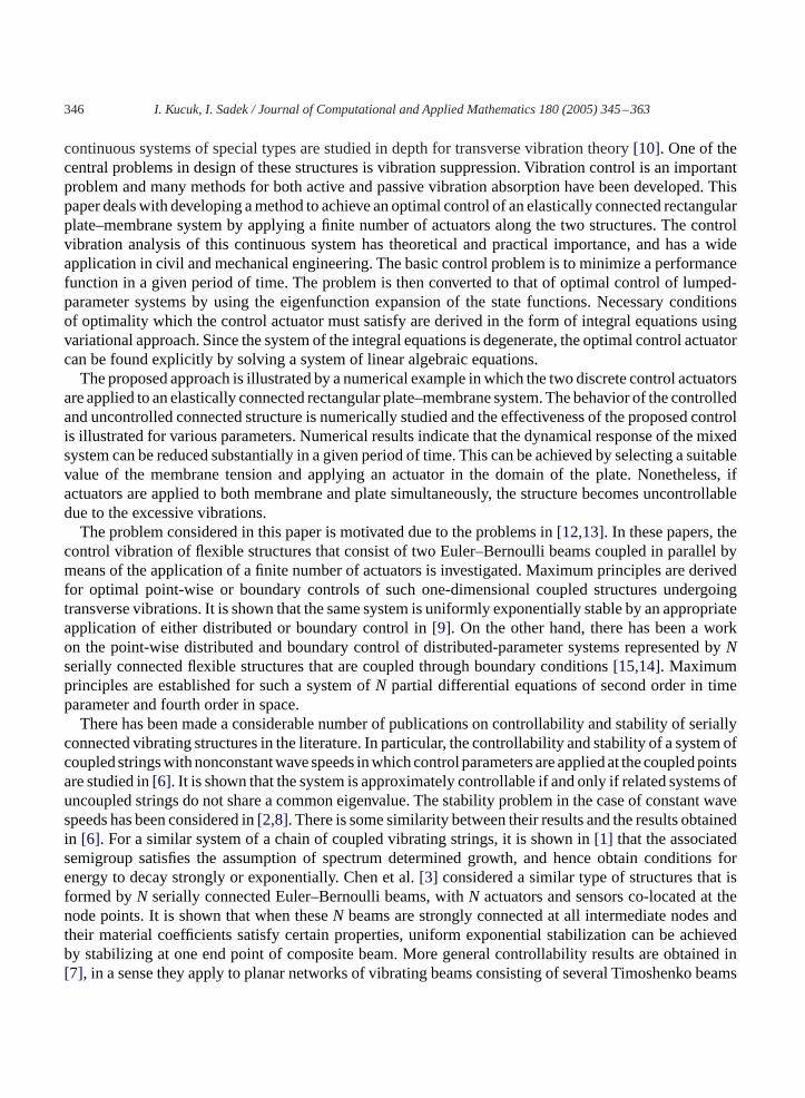
In this paper, we analyze the free transverse vibrations in a complex two-dimensional continuoussystem of plate–membrane structure. In order to prevent any unwanted resonance, we suggest a newsystem where we include actuators as control parameters. Free transverse vibrations of an elasticallyconnected rectangular plate–membrane (seeFig. 1) with discretely distributed actuators are described bythe Kirchhoff–Love plate theory in the following form of differential equations[11]:

m1w1 + D1�2w1 + k(w1 − w2) =

np∑j=1

f1j�(x − xpj , y − y

pj ), (1)

m2w2 − N2�w2 + k(w2 − w1) =nm∑j=1

f2j�(x − xmj , y − ymj ), (2)

wherew1 = w1(x, y, t) (w2 = w2(x, y, t)) is the transverse plate (membrane) displacement;�(, ) is theDirac distribution;(xpj , y

pj )and(x

mj , y

mj )are from[0, a]×[0, b], and indexesp,andmrepresent plate and

membrane, respectively, throughout this paper;fij (t) ∈ L2([0, tf ]) are the amplitude (or influence) ofdistributed actuators wherei=1,2 (the subscriptsi=1 and 2 refer to plate andmembrane, respectively);D1 is the flexural rigidity of the plate;N2 is a uniform constant tension per unit length in the membrane;E1 isYoung’s modulus of the elastic plate;k is the stiffness modulus of aWinkler elastic layer; andtf is

Fig. 1. An elastically connected rectangular plate–membrane complex system with the control parametersf1k, k = 1, . . . , npfor plate; similarly,f2k, k = 1, . . . , nm are located in the membrane.


the terminal time;

D1 = E1h31

12(1− �21), mi = �ihi, wi = �wi

�t, i = 1,2,

�2w1 = �4w1�x4

+ 2�4w1

�x2�y2+ �4w1

�y4, �w2 = �2w2

�x2+ �2w2

�y2.

The boundary conditions for the simply supported plate and membrane are introduced as

w1(0, y, t) = w1(a, y, t) = w1(x,0, t) = w1(x, b, t) = 0, (3a)

w2(0, y, t) = w2(a, y, t) = w2(x,0, t) = w2(x, b, t) = 0, (3b)

�2w1�x2

∣∣∣∣∣(0,y,t)

= �2w1�x2

∣∣∣∣∣(a,y,t)

= �2w1�y2

∣∣∣∣∣(x,0,t)

= �2w1�y2

∣∣∣∣∣(x,b,t)

= 0. (3c)

The initial conditions are taken as

wi(x, y,0) = w0i (x, y),

wi(x, y,0) = v0i (x, y) i = 1,2. (4)

In order to measure the performance of the system under the influence of the applied control forcesfij (t),we introduce the following performance index function:

J(f11, . . . , f1np , f21, . . . , f2nm) = J(F ),

where

J(F ) = 1

2

∫ b

0

∫ a

0{�1w21(x, y, tf ) + �2w

21(x, y, tf ) + �3w

22(x, y, tf ) + �4w

22(x, y, tf )}dx dy

+ 1

2

∫ tf

0

( np∑i=1

�if21i (t) +

nm∑i=1

�if22i (t)

)dt. (5)

Here in (5),�i �0 for i = 1,2,3,4 such that�1+ �2+ �3+ �4 = 0; �i �0, i = 1, . . . , np, and�i �0, i =1, . . . , nm are the weight factors that determine the influence of the distributed actuators. The first fourterms on the right-hand side of (5) are the contribution of themodified energies of the plate andmembrane,and the other two terms represent a contribution of the energy that accumulates over the control duration[0, tf ].The optimal control problem to be studied in the present work is the following:

Problem. Find an optimalf �ij (t) ∈ L2([0, tf ]) such that

J(F �(t))�J(F (t)), ∀fij (t) ∈ L2([0, tf ])subject to (1)–(5).


3. Solution method of the vibration problem

The equations in (1) and (2) with boundary conditions in (3) can be solved by the eigenfunctionexpansion technique, assuming the solutions in the form of

w1(x, y, t) =N∑m,n

�mn(x,y)︷︸︸︷�m(x)n(y) T

1mn(t)

=N∑m,n

�mn(x, y)T1mn(t), (6)

w2(x, y, t) =N∑m,n

�m(x)n(y)T2mn(t)

=N∑m,n

�mn(x, y)T2mn(t), (7)

whereT 1mn(t) and T2mn(t) are unknown time functions, andN is the number of modes taken in the

calculations and, in theory,N → ∞. However, in practice, it is customary to expand the displacementwi(x, y, t), i=1,2 with a high accuracy through the truncated forms (6)–(7), whereNmaybe rather largebut it is taken finite in this paper. Complete orthonormal sets of eigenfunctions of the operator

Lw = �2w�x2

+ �2w�y2

(8)

are obtained as

{�m(x)}∞m=1 ={√

2

asin(amx)

}∞

m=1,

{n(y)}∞n=1 ={√

2

bsin(bny)

}∞

n=1, (9)

wheream = a−1m; m = 1,2, . . . , andbn = b−1n; n = 1,2, . . . .

If one substitutes solutions (6) and (7) into (1) and (2), we obtain

N∑m,n

�mn(x, y){m1T 1mn(t) + (D1k2mn + k)T 1mn(t) − kT 2mn(t)}

=np∑j=1

f1j (t)�(x − xpj , y − y

pj )


andN∑m,n

�mn(x, y){m2T 2mn(t) + (N2kmn + k)T 2mn(t) − kT 1mn(t)}

=nm∑j=1

f2j (t)�(x − xmj , y − ymj ).

Using the orthogonal property of eigenfunctions mounts to the following second-order differential equa-tions in time; with the initial conditions given in (4):

T 1mn(t) + �1mnT1mn(t) − �10T

2mn(t) = F1(t), (10a)

T 2mn(t) + �2mnT2mn(t) − �20T

1mn(t) = F2(t), (10b)

where

�1mn = D1k2mn + k

m1; �2mn = N2kmn + k

m2; �i0 = k

mi

, i = 1,2; kmn = a2m + b2n

F1(t) = m−11

np∑j=1

f1j (t)�mn(xpj , y

pj ), F2(t) = m−1

2

nm∑j=1

f2j (t)�mn(xmj , y

mj ). (11)

To solve the coupled system of second-order differential equations in time, one can rewrite the equationsin (10) as a coupled system of first-order differential equations. To do this, we introduce new variablesymn1 ,ymn

2 ,ymn3 andymn

4 defined as

ymn1 = T 1mn(t),

ymn2 = T 1mn(t),

ymn3 = T 2mn(t),

ymn4 = T 2mn(t). (12)

From (12), it follows immediately that (10) is written as

ymn1 (t) = ymn

2 (t),

ymn2 (t) = −�1mny

mn1 (t) + �10y

mn3 (t) + F1(t),

ymn3 (t) = ymn

4 (t),

ymn4 (t) = −�2mny

mn3 (t) + �20y

mn1 (t) + F2(t), (13)

or in a more compact form

dY

dt= AY + F(t), (14)

where

Y =ymn1

ymn2

ymn3

ymn4

; A =

0 1 0 0−�1mn 0 �10 00 0 0 1

�20 0 −�2mn 0

; F(t) =

0F1(t)

0F2(t)

.


First-order systemof differential equations (FOSDE) in (13) is subjected to the following initial conditionsdue to the initial conditions (4):

ymn1 (0) = T 1mn(0) =

∫ b

0

∫ a

0�mn(x, y)w

01(x, y)dx dy, (15a)

ymn2 (0) = T 1mn(0) =

∫ b

0

∫ a

0�mn(x, y)v

01(x, y)dx dy, (15b)

ymn3 (0) = T 2mn(0) =

∫ b

0

∫ a

0�mn(x, y)w

02(x, y)dx dy, (15c)

ymn4 (0) = T 2mn(0) =

∫ b

0

∫ a

0�mn(x, y)v

02(x, y)dx dy. (15d)

Note that|A| = �1mn�2mn − �10�20>0, and the eigenvalues ofA are obtained as

�1,2 = ∓I 1; �3,4 = ∓I 2 whereI= √−1. (16)

Here 1 and 2 are defined as

1 =√

�12, and 2 =

√�22, (17)

where

�1 = �12mn − √D>0, �2 = �12mn + √

D>0, (18)

in which�12mn = �1mn + �2mn, D = (�1mn − �2mn)2 + 4�10�20. Then the corresponding eigenvectors of

A are obtained as

vi =[−�i

1,−2�1mn + �2

2�20,−ϑi

1,1

]i = 1,2; (19)

vj =[−�j

2,−2�1mn + �1

2�20,−ϑ

j2,1

]j = 3,4; (20)

where

�i1 = �i

2�20|A| ((�2mn)

2 + �2mn

√D + �10�20− |A|); ϑi

1 = 2�i�1

i = 1,2;

�j2 = �j

2�20|A| ((�2mn)

2 − �2mn

√D + �10�20− |A|); ϑ

j2 = 2�j

�2j = 3,4.

Since the matrixA in (14) has four distinct eigenvalues,A is diagonalizable matrix. To find the solutionof the system given in (14), we define a matrixB whose columns are the eigenvectorsv1, v2, v3, andv4ofA and introduce a new dependent variableX with

Y = BX. (21)

Substituting this new variable forY into (14) amounts to

X = (B−1AB)X + B−1F(t)

=DX +G(t), (22)


whereD = B−1AB is diagonal matrix with the eigenvalues ofA are on the main diagonal, andG(t) =B−1F(t) defined as

G(t) = �

11

−1−1

F1(t) +

�1�1�2�2

F2(t) (23a)

=G1F1(t) +G2F2(t), (23b)

where

� = �20

2√D, �1 = 2�1mn − �1

4√D

�2 = −2�1mn − �2

4√D

.

Eq. (22) is a system of four uncoupled differential equations forXmni (t), i =1,2,3,4. In scalar form, we

observe the following equations:

dXmni (t)

dt= �iX

mni (t) + Gi(t) (24)

with the proper form of the initial conditions given in (15). The solutions of FOSDE of (13) are of thefollowing form:

Xmni (t) = e�i t

∫ t

0e−�i sGi(s)ds + cie

�i t , (25)

whereci are constants to be determined by the initial conditions given (15).The solution of (13) is given as

Xmn1 (t) = eI 1t

�m−1

1

np∑j=1

�mn(xpj , y

pj )

∫ t

0f1j (s)e

−I 1s ds

+ �1m−12

nm∑j=1

�mn(xmj , y

mj )

∫ t

0f2j (s)e

−I 1s ds

+ c1e

I 1t ,

Xmn2 (t) = e−I 1t

�m−1

1

np∑j=1

�mn(xpj , y

pj )

∫ t

0f1j (s)e

I 1s ds

+ �1m−12

nm∑j=1

�mn(xmj , y

mj )

∫ t

0f2j (s)e

I 1s ds

+ c2e

−I 1t ,


Xmn3 (t) = eI 3t

−�m−1

1

np∑j=1

�mn(xpj , y

pj )

∫ t

0f1j (s)e

−I 3s ds

+ �2m−12

nm∑j=1

�mn(xmj , y

mj )

∫ t

0f2j (s)e

−I 3s ds

+ c3e

I 3t ,

Xmn4 (t) = e−I 3t

−�m−1

1

np∑j=1

�mn(xpj , y

pj )

∫ t

0f1j (s)e

I 3s ds

+ �2m−12

nm∑j=1

�mn(xmj , y

mj )

∫ t

0f2j (s)e

I 3s ds

+ c4e

−I 3t . (26)

In (26), the constantsc are defined as

ci = Xmni (0) =

4∑j=1

bijymnj (0) i = 1,2,3,4, (27)

wherebij are the terms from the inverse ofB given in (21), andymnj (0) are given in (15).

Finally, we are ready to write the solutions forT 1mn andT2mn, and their derivatives:

T 1mn(t) =4∑

j=1b1jX

mnj (t), (28)

T 1mn(t) =4∑

j=1b2jX

mnj (t), (29)

T 2mn(t) =4∑

j=1b3jX

mnj (t), (30)

T 2mn(t) =4∑

j=1b4jX

mnj (t). (31)

Thus, the deflections in plate and membrane are obtained as

w1(x, y, t) =N∑mn

�mn(x, y)

4∑j=1

b1jXmnj (t), (32)

w2(x, y, t) =N∑mn

�mn(x, y)

4∑j=1

b3jXmnj (t), (33)

whereB = [bij ]4×4 whose columns are the eigenvectors ofA, andXmnj (t) are defined in (26).


4. Necessary conditions of optimality

In this section, we will derive the necessary conditions of optimality for the applied actuators in thedomain of the plate and membrane. It should be noticed that the deflections and the velocities of theplate and membrane are functions of the actuators. To find the optimal control parameters, the optimalactuators, for the performance index defined in (5), we fix the membrane tension, the location of theactuators in the domain, and weight factors and differentiate (5) with respect tof1k, k = 1, . . . , np andf2k, k = 1, . . . , nm.First, we observe the following fact with help of orthonormality of the eigenfunctions:

∫ b

0

∫ a

0w2i (x, y, tf )dx dy =

∫ b

0

∫ a

0

[N∑mn

�mn(x, y)Timn(tf )

]2dx dy

=N∑mn

(T imn(tf ))

2. (34)

The solutions of (1) and (2) given in (32) and (33), respectively, and the obtained result in (34) rewritethe performance index function as

J(F ) = 1

2

N∑mn

4∑i=1

�i

4∑

j=1bijX

mnj (tf )

2 + 1

2

∫ tf

0

( np∑i=1

�if21i(t) +

nm∑i=1

�if22i(t)

)dt. (35)

We now proceed directly by taking the first variation of (35) with respect tof1k

�f1k =∫ tf

0

N∑mn

4∑i=1

�i

4∑

j=1bijX

mnj (tf )

×4∑

j=1bije

�j (tf −s)G1j�mn(xpk , y

pk )�f1k + �kf1k(s)

�f1k(s)ds = 0. (36)

Here the derivative ofXmnj (tf ; f1k, f2k) with respect tof1k is

(Xmnj (tf ))f1k =

∫ tf

0e�j (tf −s)G1j�mn(x

pk , y

pk )�f1k(s)ds. (37)


Since (36) is true for all variations of�f1k, we observe the following for fixedk = 1, . . . , np:

N∑mn

4∑i=1

�i

4∑j=1

bij

∫ tf

0e�j (tf −r)

G1j np∑

q=1f1q(r)�mn(x

pq , y

pq )

+G2j

nm∑q=1

f2q(r)�mn(xmq , y

mq )

dr + cje

�j tf

× 4∑j=1

bije�j (tf −s)G1j�mn(x

pk , y

pk )

+ �kf1k(s) = 0, (38)

whereG1j andG2j are the terms from the column coefficient matrices ofF1(t) andF2(t) given in(23b), and(xpi , y

pi ) and(x

mi , y

mi ) are the points at which the control actuators are located for plate and

membrane, respectively.We obtain the similar result from the variation ofJ(F ) with respect tof2k for fixedk = 1, . . . , nm:

N∑mn

4∑i=1

�i

4∑

j=1bij

∫ tf

0e�j (tf −r)

G1j np∑

q=1f1q(r)�mn(x

pq , y

pq )

+G2j

nm∑q=1

f2q(r)�mn(xmq , y

mq )

dr + cje

�j tf

× 4∑

j=1bije

�j (tf −s)G2j�mn(xmk , y

mk )

+ �kf2k(s) = 0. (39)

Eqs. (38) and (39) can be written in a more compact form so that coupled nonhomogeneous Fredholmintegral equations with degenerate kernel can be observed for each fixedk as

N∑mn

np∑q=1

4∑i=1

∫ tf

0(K qk

imn(s)f1q(r) + Kqk

imn(s)f2q(r))e�i (tf −r) dr + Pkmn(s)

+ �kf1k(s) = 0, (40a)

N∑mn

nm∑q=1

4∑i=1

∫ tf

0(Lqk

imn(s)f1q(r) + Lqk

imn(s)f2q(r))e�i (tf −r) dr + P

k

mn(s)

+ �kf2k(s) = 0. (40b)

In (40), K (s) = diag(G1)BTdiag(�1, �2, �3, �4)(KK )4×1(s)�mn(xpk , y

pk ) where (KK )4×1(s) =

(∑4

j=1 bijG1je(tf −s)�j )4×1. The other terms in (40) can be obtained similarly.


If we definecqi andcqi as the integrals in (40),

cqi =

∫ tf

0e�i (tf −r)f1q(r)dr, (41a)

cqi =

∫ tf

0e�i (tf −r)f2q(r)dr, (41b)

then (40)’s become

N∑mn

np∑q=1

4∑i=1

(K qkimn(s)c

qi + K

qk

imn(s)cqi ) + Pkmn(s)

+ �kf1k(s) = 0, (42a)

N∑mn

nm∑q=1

4∑i=1

(Lqkimn(s)c

qi + L

qk

imn(s)cqi

)+ P

k

mn(s)

+ �kf2k(s) = 0, (42b)

wherek=1, . . . , np in (42a) andk=1, . . . , nm in (42b). If we multiply all terms of (42) by e�l (tf −s) andintegrate from 0 totf , one obtains a system of linear equations inc

qi andc

qi :

N∑mn

np∑q=1

4∑i=1

(alqikmnc

qi + b

lqikmnc

qi ) + hlkmn

+ �kc

lk = 0, k = 1, . . . , np, (43a)

N∑mn

nm∑q=1

4∑i=1

(alqikmnc

qi + b

lq

ikmncqi ) + h

l

kmn

+ �kc

lk = 0, k = 1, . . . , nm, (43b)

where 1� l�4, and

alqikmn =

∫ tf

0K qk

imn(s)e�l (tf −s) ds,

alqikmn =

∫ tf

0K

qk


hlkmn =∫ tf

0Pkmn(s)e

�l (tf −s) ds,

blqikmn =

∫ tf

0Lqkimn(s)e

�l (tf −s) ds,

blq

ikmn =∫ tf

0Lqk


hl

kmn =∫ tf

0Pk

mn(s)e�l (tf −s) ds.

Now we reach at the system of linear equations forcqi andc

qi . In order to solve these linear equations,

we assumenp = nm but this does not mean we apply the actuators at the same locations in the plate and


membrane. Eq. (43) can be written in the following compact form of system of linear equations:

(A + IE)C + AC + H = O,

BC + (B + IS)C + H = O. (44)

Here in (44), we obtain a system of linear equations for the unknownC andC that are defined as 4np ×1column block matrices. The matrices used in (44) are defined explicitly in Appendix A, and solutions aregiven as(

C

C

)4np×1

=(

A + IE A

B B + IS

)−1

4np×4np

(H

H

)4np×1

.

After computingC andC, we can computef1q andf2q by substituting (41) into (42):

f1k(s) = − 1

�k

N∑mn

Pkmn(s) +

np∑q=1

4∑i=1

(K qkimn(s)c

qi + K

qk

imn(s)cqi )

, (45a)

f2k(s) = − 1

�k

N∑mn

Pkmn(s) +

np∑q=1

4∑i=1

(Lqkimn(s)c

qi + L

qk

imn(s)cqi )

, (45b)

wherek = 1, . . . , np.With these results in (45), we find the optimal control parameters in the structurefor a fixed membrane tensionN2 and location of the actuators.

5. Numerical example

To illustrate theoretical considerations presented in this paper, the behavior of uncontrolled and con-trolled plate–membrane system is investigated. Moreover, the effect of various problem parameters onthe control of the motion in the plate–membrane system is discussed. For the simplicity of the analysis,it is assumed that the plate–membrane system is subjected to the initial conditions (4) of the form:

wi(x, y,0) = �11(x, y),

wi(x, y,0) = 0 i = 1,2, (46)

i.e., fundamental mode of the system is taken in (6)–(7). The initial conditions given in (46) allow us tostudy the behavior of the fundamental mode of the complex mixed continuous system. The measure ofthe force spent in the control process is taken as

C(t) =∫ t

0f 21 1(s)ds (47)

and the modified energy for the system is defined to be

E(N2, f11, f21) = 1

2

∫ a

0

∫ b

0

{�1w

21(x, y, tf ) + �2w

21(x, y, tf )

+ �3w22(x, y, tf ) + �4w

22(x, y, tf )

}dx dy. (48)


Table 1Energy (E(N2, f11, f21)) defined in (48) in the system &N2

N2 Energy Reduction(%)

Before control After control

0 9.9005 10.6304 N/A50 1.6759 1.2882 23.13100 5.3742 5.1140 4.85150 5.4842 5.2008 5.16200 0.5163 0.0254 95.08

Thevaluesof theparameterscharacterizing thephysical andgeometrical propertiesof theplate–membranesystem from Ref.[11] are used in the numerical calculations:

a = 1, b = 2, k = 1× 104, E1 = 1× 108, h1 = 1× 10−2, h2 = 4× 10−3,m1 = 50, m2 = 1, tf = 5, �1 = 0.3, �1 = 5× 103, �2 = 2.5× 102.In the numerical results, the deflection, velocity and the force functions are given at a point(x, y). In

Table 1, the effect of the forces acting on both plate and membrane at the points(xp1 , y

p1 )= (0.6,0.6) and

(xm1 , ym1 )= (0.8,1.8) are presented. It is observed from theTable 1that the system achieves a substantial

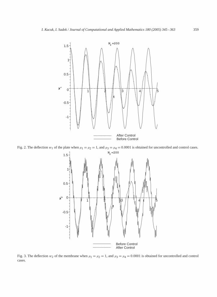
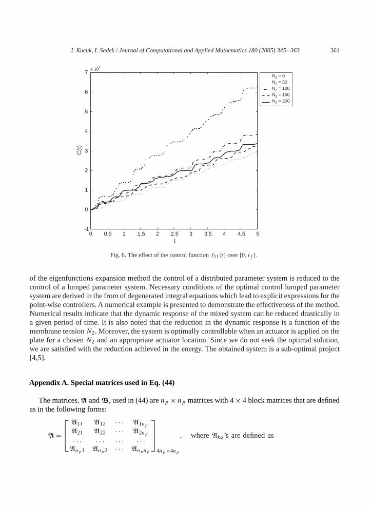
reduction in the energy when only one controller is applied to plate withN2 = 200. The system isuncontrollable (seeFig. 6) when the two controllers are applied on both plate and membrane, or only themembrane. It is also observed that the changing of the membrane tensionN2 has an evident influence onthe frequencies of the system and can be used to suppress excessive vibration amplitudes, whilst othergeometrical and physical parameters of the system can remain unchanged.For one actuator applied on the plate withmembrane tensionN2=200,Figs. 2and3show that the peak

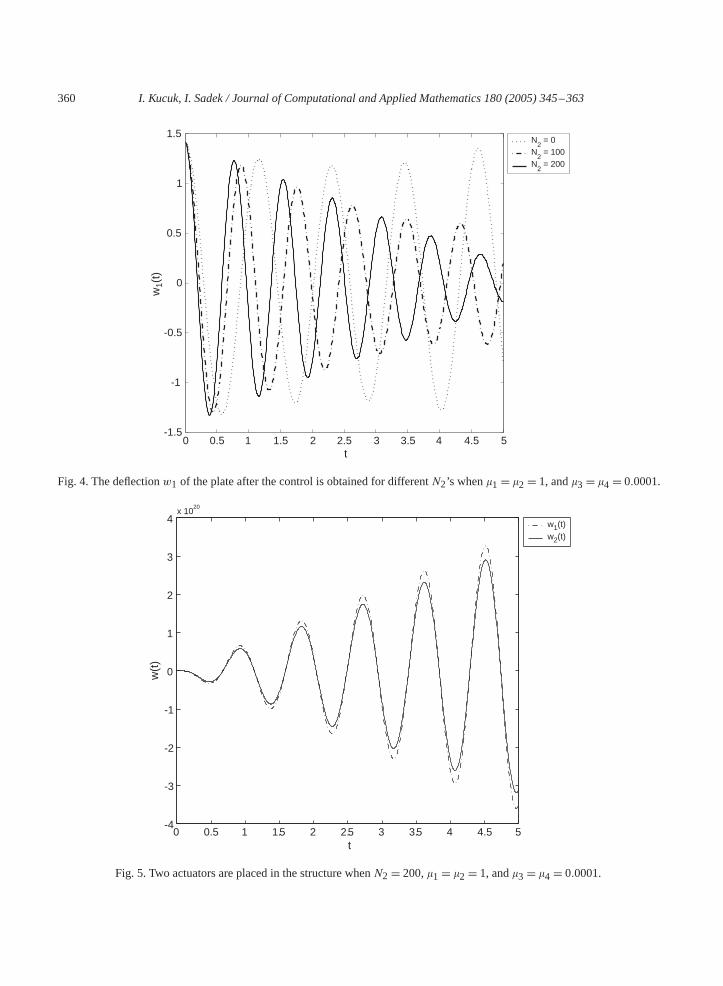
displacement of the plate and membrane is reduced substantially as compared to the uncontrolled plateand membrane, respectively. It follows fromFig. 4that varyingN2 gives different vibration reductions inthe plate as well as in the membrane. It should be that the natural frequencies of the systemmaybe variedwith a change of membrane tensionN2 without necessity to vary parameters characterizing physical andgeometrical properties of the system. This possibility is of great important factor in controlling the systemas it is observed inFig. 4. The effect of the application of each actuator on the plate and membrane isillustrated inFig. 5. It shows that applying control actuators on the plate and membrane destabilizes thesystem. As expected, the total effect of the control actuatorC(t) in (47) increases ast increases, and itsbehavior can be seen inFig. 6.

6. Conclusion

In this paper, control vibrations of an elastically connected rectangular plate–membrane system isconsidered. The vibratory system model is composed of a thin plate, a massless elastic layer modelledas a homogeneous Winkler-type foundation, and a parallel membrane stretched uniformly by suitableconstant tensions applied at the edges. A method is proposed to damp the undesirable vibrations in thestructure actively by means of control actuators applied in the domain of the structures. Upon the use


After ControlBefore Control

=2002N

1w

-1

-0.5

0

0.5

1

1.5

1 2 3 4 5

t

Fig. 2. The deflectionw1 of the plate when�1= �2 = 1, and�3= �4= 0.0001 is obtained for uncontrolled and control cases.

Before ControlAfter Control

=2002N

2w

-1

-0.5

0

0.5

1

1.5

1 2 3 4 5

t

Fig. 3. The deflectionw2 of the membrane when�1 = �2 = 1, and�3 = �4 = 0.0001 is obtained for uncontrolled and controlcases.


0 0.5 1 1.5 2 2.5 3 3.5 4 4.5 5-1.5

-1

-0.5

0

0.5

1

1.5

t

w1(

t)N

2 = 0

N2 = 100

N2 = 200

Fig. 4. The deflectionw1 of the plate after the control is obtained for differentN2’s when�1= �2 = 1, and�3= �4= 0.0001.

0 0.5 1 1.5 2 2.5 3 3.5 4 4.5 5-4

-3

-2

-1

0

1

2

3

4x 10

20

t

w(t

)

w1(t)w2(t)

Fig. 5. Two actuators are placed in the structure whenN2 = 200,�1= �2 = 1, and�3= �4= 0.0001.


0 0.5 1 1.5 2 2.5 3 3.5 4 4.5 5-1

0

1

2

3

4

5

6

7x 10

4

t

C(t

)N2 = 0N2 = 50N2 = 100N2 = 150N2 = 200

Fig. 6. The effect of the control functionf11(t) over[0, tf ].

of the eigenfunctions expansion method the control of a distributed parameter system is reduced to thecontrol of a lumped parameter system. Necessary conditions of the optimal control lumped parametersystem are derived in the from of degenerated integral equations which lead to explicit expressions for thepoint-wise controllers. A numerical example is presented to demonstrate the effectiveness of the method.Numerical results indicate that the dynamic response of the mixed system can be reduced drastically ina given period of time. It is also noted that the reduction in the dynamic response is a function of themembrane tensionN2. Moreover, the system is optimally controllable when an actuator is applied on theplate for a chosenN2 and an appropriate actuator location. Since we do not seek the optimal solution,we are satisfied with the reduction achieved in the energy. The obtained system is a sub-optimal project[4,5].

Appendix A. Special matrices used in Eq. (44)

The matrices,A andB, used in (44) arenp × np matrices with 4× 4 block matrices that are definedas in the following forms:

A =A11 A12 · · · A1npA21 A22 · · · A2np. . . . . . . . . . . .

Anp1 Anp2 · · · Anpnp

4np×4np

, whereAkq ’s are defined as


Akq =

N∑mn

a1q1kmn

N∑mn

a1q2kmn

N∑mn

a1q3kmn

N∑mn

a1q4kmn

N∑mn

a2q1kmn

N∑mn

a2q2kmn

N∑mn

a2q3kmn

N∑mn

a2q4kmn

N∑mn

a3q1kmn

N∑mn

a3q2kmn

N∑mn

a3q3kmn

N∑mn

a3q4kmn

N∑mn

a4q1kmn

N∑mn

a4q2kmn

N∑mn

a4q3kmn

N∑mn

a4q4kmn

where 1�k�np and 1�q�np;

B =B11 B12 · · · B1npB21 B22 · · · B2np. . . . . . . . . . . .

Bnp1 Bnp2 · · · Bnpnp

4np×4np

,whereBkq ’s are defined as

Bkq =

N∑mn

b1q1kmn

N∑mn

b1q2kmn

N∑mn

b1q3kmn

N∑mn

b1q4kmn

N∑mn

b2q1kmn

N∑mn

b2q2kmn

N∑mn

b2q3kmn

N∑mn

b2q4kmn

N∑mn

b3q1kmn

N∑mn

b3q2kmn

N∑mn

b3q3kmn

N∑mn

b3q4kmn

N∑mn

b4q1kmn

N∑mn

b4q2kmn

N∑mn

b4q3kmn

N∑mn

b4qXS4kmn

where 1�k�np and 1�q�np.

The unknownC andC are defined as 4np × 1 column matrices of block matrices:

C =

C1

C2...

Cnp

whereCi =

ci1ci2ci3ci4

; C =

C1

C2

...

Cnp

whereC

i =

ci1ci2ci3ci4

.

Finally, I is annp × np identity matrix with 4× 4 identity matrices in the main diagonal.

I =I4×4 0 . . . 00 I4×4 . . . 0. . .

0 0 . . . I4×4

np×np

.

HereI4×4 are 4× 4 identity matrices,

E =

E1E2...

Enp

, whereEi =

�i�i�i�i

and S =

S1S2...

Snp

whereSi =

�i�i�i�i

.


References

[1] W.L. Chan, G.B. Zhu, Pointwise stabilization for a chain of coupled vibrating strings, IMA J. Math. Control Inform. 7(1990) 307–315.

[2] G. Chen, M. Coleman, H. West, Pointwise stabilization in the middle of the span for second order systems, nonuniformand uniform exponential decay of solutions, SIAM J. Appl. Math. 47 (4) (1987) 751–780.

[3] G. Chen, M. Delfour, A.M. Krall, G. Payre, Modelling, stabilization and control of serially connected beams, SIAM J.Control Optim. 25 (3) (1987) 526–535.

[4] A.V. Cherkaev, Variational Methods for Structural Optimization, vol. 140, Springer, NewYork, Berlin, Heidelberg, 2000.[5] A.V. Cherkaev, I. Kucuk, Detecting stress fields in an optimal structure part I: two-dimensional case and analyzer, Struct.

Multidiscip. Optim. 26 (1–2) (2004) 1–15.[6] L. Ho, Controllability and stability of coupled strings with control applied points, SIAM J. Control Optim. 31 (1993) 1416

–1437.[7] J.E. Lagnese, G. Leugering, E.J.P.G. Schmidt, Control of planar networks of Timoshenko beams, SIAM J. Control Optim.

31 (3) (1993) 780–811.[8] K. Liu, F. Huang, G. Chen, Exponential stability analysis of a long chain of coupled vibrating strings with dissipative

linkage, SIAM J. Appl. Math. 49 (1989) 1694–1707.[9] M. Najafi, R. Sarhangi, H.Oloomi, Distributed and boundary control for a parallel of Euler-Bernoulli beams, J.Vib. Control

3 (1997) 183–199.[10] Z.Oniszczuk,Vibration analysis of the compoundcontinuous systemswith elastic constraints,TechnicalReport, Publishing

house of Rzeszow University of Technology, 1997 (in Polish).[11] Z. Oniszczuk, Free transverse vibrations of an elastically connected rectangular plate-membrane complex system, J. Sound

Vib. 264 (2003) 37–47.[12] I. Sadek, M.Abukhaled, T.Abualrub, Optimal pointwise control for a parallel system of Euler-Bernoulli beams, J. Comput.

Appl. Math. 137 (1) (2001) 83–95.[13] I. Sadek, T. Abualrub, M. Abukhaled, Optimal boundary control of systems of elastically connected parallel beams,

Dynamics Continuous, Discrete Impulsive Systems, to appear.[14] I. Sadek, L. Jamiiru, H. Al-Mohamad, Optimal boundary control of one-dimensional multi-span vibrating systems, J.

Comput. Appl. Math. 94 (1) (1998) 39–54.[15] I. Sadek, V. Melvin, Optimal control of serially connected structures using spatially distribute pointwise controllers, IMA

J. Math. Control Inform. 13 (4) (1996) 335–358.

Documents

Optimal control of an elastically connected rectangular plate–membrane system