Title Wrinkle generation in shear-enforced rectangular membrane

Author(s) Senda, Kei; Petrovic, Mario; Nakanishi, Kei

Citation Acta Astronautica (2015), 111: 110-135

Issue Date 2015-06

URL http://hdl.handle.net/2433/196845

Right

© 2015 IAA. Published by Elsevier Ltd. NOTICE: this is theauthor's version of a work that was accepted for publication inActa Astronautica. Changes resulting from the publishingprocess, such as peer review, editing, corrections, structuralformatting, and other quality control mechanisms may not bereflected in this document. Changes may have been made tothis work since it was submitted for publication. A definitiveversion was subsequently published in Acta Astronautica,111(2015) doi:10.1016/j.actaastro.2015.02.022; この論文は出版社版でありません。引用の際には出版社版をご確認ご利用ください。This is not the published version. Please citeonly the published version.

Type Journal Article

Textversion author

Kyoto University

Wrinkle Generation in Shear-Enforced RectangularMembrane

Kei Senda1,∗, Mario Petrovic2, Kei Nakanishi2

Kyoto University, Kyoto daigaku-Katsura, Nishikyo-ku, Kyoto 615-8530, Japan

Abstract

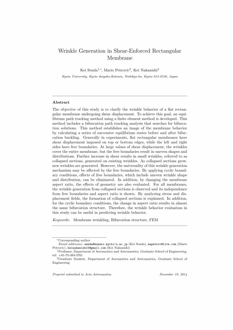
The objective of this study is to clarify the wrinkle behavior of a flat rectan-gular membrane undergoing shear displacement. To achieve this goal, an equi-librium path tracking method using a finite element method is developed. Thismethod includes a bifurcation path tracking analysis that searches for bifurca-tion solutions. This method establishes an image of the membrane behaviorby calculating a series of successive equilibrium states before and after bifur-cation buckling. Generally in experiments, flat rectangular membranes haveshear displacement imposed on top or bottom edges, while the left and rightsides have free boundaries. At large values of shear displacement, the wrinklescover the entire membrane, but the free boundaries result in uneven shapes anddistributions. Further increase in shear results in small wrinkles, referred to ascollapsed sections, generated on existing wrinkles. As collapsed sections grow,new wrinkles are generated. However, the universality of this wrinkle generationmechanism may be affected by the free boundaries. By applying cyclic bound-ary conditions, effects of free boundaries, which include uneven wrinkle shapeand distribution, can be eliminated. In addition, by changing the membraneaspect ratio, the effects of geometry are also evaluated. For all membranes,the wrinkle generation from collapsed sections is observed and its independencefrom free boundaries and aspect ratio is shown. By analyzing stress and dis-placement fields, the formation of collapsed sections is explained. In addition,for the cyclic boundary conditions, the change in aspect ratio results in almostthe same bifurcation structure. Therefore, the wrinkle behavior evaluation inthis study can be useful in predicting wrinkle behavior.

Keywords: Membrane wrinkling, Bifurcation structure, FEM

∗Corresponding authorEmail addresses: senda@kuaero.kyoto-u.ac.jp (Kei Senda), mapetrov@live.com (Mario

Petrovic), keinakanishi5@gmail.com (Kei Nakanishi)1Professor, Department of Aeronautics and Astronautics, Graduate School of Engineering,

tel: +81-75-383-37612Graduate Student, Department of Aeronautics and Astronautics, Graduate School of

Engineering

Preprint submitted to Acta Astronautica December 19, 2014

1. Introduction

When the structure and design of space vehicles are considered, weight andstorage requirements are key limiting factors. Inflatable structures have at-tracted attention because such structures satisfy the above factors[1]. This studyconsiders structures using deployable membranes. The structures are initiallyfolded, deployed into their desired shape, unfolded or inflated, and rigidized.

The research goal of this study is to achieve stable deployment along aplanned trajectory for a structure folded into a prescribed shape. However, be-cause the structure is a membrane, with many degrees of freedom, the predictionof membrane behavior is difficult. Here membrane behavior refers to displace-ment of membrane points under the effect of external loads. In a deploymentexperiment using an inflatable tube[2], an origami-like pattern was designed tofacilitate predictable deployment. However, small compressive forces cause localbuckling and generates wrinkles. Buckling occurs after a bifurcation[3, 4, 5, 6].When the bifurcation occurs, the material may become unstable and the sub-sequent state may not be uniquely determined. This makes predicting stabledeployment difficult. To solve this problem, understanding of wrinkle behavioris essential.

Buckling results in a finite deformation occurring in a direction differentfrom the direction of the load applied to the structure. In this study, a wrinklerepresents this finite deformation. Therefore, a wrinkle is defined as an out-of-plane membrane deformation that occurs when a compressive load is applied toa membrane.

An equilibrium state, or an equilibrium point, is defined as the static stateof a membrane when a static load or an imposed displacement is applied. Byvarying a path parameter such as displacement or load, an equilibrium path isobtained, i.e. successive equilibrium points. Bifurcation is a rapid equilibriumpoint shift and a qualitative change of the equilibrium state when the pathparameter varies. A wrinkle, i.e. buckling of a membrane, is generated after abifurcation. Therefore, in order to deploy a membrane structure along a plannedtrajectory, understanding of the bifurcation structure and the equilibrium pathsis necessary.

The first step in analyzing wrinkling behavior is modeling the membranestructure. A continuum model based on partial differential equations and aFinite Element (FE) model are typical approaches, however the former yieldssolutions for only simple systems. Therefore, finite element modeling is usedto analyze wrinkle behavior. In previous studies[7, 8, 9], membrane structureswere modeled with the membrane elements that ignore bending stiffness. Themembrane elements approach excels in terms of computational cost, howeverit can not accurately calculate the out-of-plane deformation. By using shellelements that include bending stiffness, wrinkle amplitude and wavelength aremore accurately calculated.

In a straight column or flat plate, the bifurcation after which buckling occursis a branching bifurcation[3, 10]. For a flat membrane, it is believed that awrinkle is generated by bifurcation. Therefore the number of wrinkles increases

2

after bifurcation. A bifurcation is a singularity in the analysis. Therefore,obtaining equilibrium points after bifurcation is difficult and numerous studieshave been conducted[11]. A method for bifurcation path analysis is needed toobtain equilibrium points after bifurcation.

The arc length method, the introduction of imperfections and dynamic anal-ysis, are the common methods for path tracking after bifurcations[12, 6]. How-ever, these methods do not always yield a solution, they change the bifurcationstructure, or they obtain a fraction of paths after the bifurcation. To over-come this problem, a bifurcation path analysis method that is able to searchfor solutions after bifurcation is needed. In this study, a method of searchingfor bifurcation solutions is added into the equilibrium path tracking method, ofWagner and Wriggers[13].

Membrane wrinkling studies have mostly focused on certain effects on char-acteristics, i.e. gravity[14], creases[15], stress concentrations[16], etc. In general,wrinkling is analyzed as a membrane behavior event, and wrinkled geometry iscomputed for specific loads. The goal of this study is to obtain a comprehensiveimage/understanding of membrane wrinkling. For that purpose, several wrin-kle generations, multiple wrinkle configurations, and wrinkle interaction will beconsidered.

In previous studies[4, 17], a flat rectangular membrane with free boundaryconditions was sheared. In Wong and Pellegrino[5, 6], a wide range of numericalresults were shown. In addition, Senda, et al. [22] showed the wrinkle behav-ior for relatively small values of imposed shear. The membrane becomes fullywrinkled for small values of shear. However, it was also shown that the shapeand distribution of the wrinkles is not uniform due to the influence of the thefree boundaries.

In this study, by increasing the shear displacement in a fully wrinkled mem-brane, the wrinkle behavior, and the mechanism behind it, is shown. Theincrease in shear displacement results in small wrinkles generated near the fixedboundaries on existing wrinkles. These small wrinkles will be referred as col-lapsed sections to distinguish them from the larger, existing wrinkles. By in-creasing the shear displacement further, the collapsed sections expand along thelength of existing wrinkles. At a critical size, the sections perform an unstableexpansion, they join in the middle of the existing wrinkle, split it and resultin two new wrinkles. This behavior repeats with further increase in shear andrepresents the basic behavior for wrinkle increase when the membrane is fullywrinkled.

Originally, this behavior is observed for a membrane with an aspect ratio of3:1 and free boundary conditions. Therefore, it is possible that this membranebehavior is a result of the free boundary effects, and therefore, it may not beuniversal. To eliminate the effects of free boundaries, in this study the mem-brane is modeled with cyclic boundaries. Furthermore, to evaluate the effectsof geometry, the cyclic boundary membrane is modeled with the aspect ratio of1:1. For all the membranes, the above described behavior of wrinkle generationby collapsed sections is observed, independently of the boundaries and aspectratio. Additionally, the behavior of collapsed sections will be explained in detail

3

through displacement and stress analysis.The rest of this paper is organized as follows. Section 2 sets up the FEM

model of the rectangular membrane using ABAQUS, a FEM software pack-age, the path analysis method and the asymptotic theory to a load parameter.Section 3 shows the path tracking method for a system with an imposed dis-placement. Section 4 introduces the similarity value and bifurcation diagram.Section 5 presents some numerical simulations and discusses the results. Section6 offers some concluding remarks.

2. Modeling and problem

2.1. Analyzed object and modelThe membrane analyzed in this study is a flat membrane as illustrated in

Fig. 1. The material is Kapton and its properties are listed in Table 1. Thechoice of a Kapton membrane comes from the flat membrane wrinkling data,e.g. Wong and Pellegrino[4] and Inoue[17]. The ratio of the horizontal and thevertical lengths a : b is 3 : 1. Fixed boundaries are set for the top and bottomedges, and cyclic boundaries for the left and right edges. The fixed top edge isthen subjected to prescribed displacement. Gravity and imperfections are notconsidered.

In this study, 3 different membranes will be used to discuss the results;a : b = 3 : 1 with cyclic boundary conditions, a : b = 3 : 1 with free boundaryconditions, and a : b = 1 : 1 with cyclic boundary conditions. The maindiscussion is based on a membrane with an aspect ratio of a : b = 3 : 1 withcyclic boundary conditions, and unless specified otherwise, the discussion refersto this model.

The origin of the xyz-coordinate system is fixed at the membrane center ofmass in the undeformed state, i.e. when no external loads are applied. The x-axis is parallel to the bottom edge, y-axis is perpendicular to the bottom edge,and z-axis is normal to the neutral plane, as defined in Fig. 1. Coordinates(x, y, z) refer to a position on the membrane prior to deformation, and theydo not vary with deformation. Section AA’ is defined at y = 0[m] and BB’ aty = −0.045[m].

First, at the top fixed edge, a displacement of δuy = 30 × 10−6[m] is appliedin the y-direction and is constant throughout the analysis. This is to maintain

Table 1: Membrane material properties.

Membrane width a 0.30 [m]Membrane height b 0.10 [m]

Membrane thickness h 12.5×10−6 [m]Young’s Modulus E 3.0 [GPa]

Poisson’s ratio ν 0.3

4

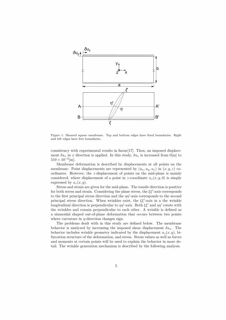
Figure 1: Sheared square membrane. Top and bottom edges have fixed boundaries. Rightand left edges have free boundaries.

consistency with experimental results in Inoue[17]. Then, an imposed displace-ment δux in x direction is applied. In this study, δux is increased from 0[m] to510 × 10−6[m].

Membrane deformation is described by displacements at all points on themembrane. Point displacements are represented by (ux, uy, uz) in (x, y, z) co-ordinates. However, the z-displacement of points on the mid-plane is mainlyconsidered, where displacement of a point in z-coordinate uz(x, y, 0) is simplyexpressed by uz(x, y).

Stress and strain are given for the mid-plane. The tensile direction is positivefor both stress and strain. Considering the plane stress, the ξξ′-axis correspondsto the first principal stress direction and the ηη′-axis corresponds to the secondprincipal stress direction. When wrinkles exist, the ξξ′-axis in a the wrinklelongitudinal direction is perpendicular to ηη′-axis. Both ξξ′ and ηη′ rotate withthe wrinkles and remain perpendicular to each other. A wrinkle is defined asa sinusoidal shaped out-of-plane deformation that occurs between two pointswhere curvature in η-direction changes sign.

The problems dealt with in this study are defined below. The membranebehavior is analyzed by increasing the imposed shear displacement δux. Thebehavior includes wrinkle geometry indicated by the displacement uz(x, y), bi-furcation structure of the deformation, and stress. Stress values as well as forcesand moments at certain points will be used to explain the behavior in more de-tail. The wrinkle generation mechanism is described by the following analysis.

5

2.2. Differential equationsThe first step in the analysis of membrane wrinkling is establishing the gov-

erning equations for plates[3]. These equations provide the key properties ofthe system. For membranes, the Kirchhoff-Love assumptions for thin plates areadopted. By taking the standard plate definitions[3] the plate equations arewritten as:

Eh

1 − ν2

[∂2ux

∂x2 + ∂uz

∂x

(∂2uz

∂x2

)+ ν

{∂2uy

∂x∂y+ ∂uz

∂y

∂2uz

∂x∂y

}]+ Eh

2(1 + ν)

{∂2ux

∂y2 + ∂2uy

∂x∂y+ ∂2uz

∂x∂y

∂uz

∂y+ ∂uz

∂x

∂2uz

∂y2

}= fx(ux, uy, uz) = 0 (1)Eh

1 − ν2

[∂2ux

∂y2 + ∂uz

∂y

(∂2uz

∂y2

)+ ν

{∂2ux

∂x∂y+ ∂uz

∂x

∂2uz

∂x∂y

}]+ Eh

2(1 + ν)

{∂2uy

∂x2 + ∂2ux

∂x∂y+ ∂2uz

∂x∂y

∂uz

∂x+ ∂uz

∂y

∂2uz

∂x2

}= fy(ux, uy, uz) = 0 (2)

− D

(∂4uz

∂x4 + ν∂4uz

∂x2∂y2

)− 2D(1 − ν) ∂4uz

∂x2∂y2 − D

(∂4uz

∂y4 + ν∂4uz

∂x2∂y2

)+ Eh

1 − ν2

{∂2ux

∂x2 + ∂2uz

∂x2 + ν

(∂2ux

∂x∂y+ ∂uz

∂y

∂2uz

∂x∂y

)}∂uz

∂x

+ Eh

2(1 + ν)

(∂2ux

∂x∂y+ ∂2uy

∂x2 + ∂2uz

∂x2∂uz

∂y+ ∂uz

∂x

∂2uz

∂x∂y

)∂uz

∂y

+ Eh

1 − ν2

{∂2ux

∂y2 + ∂uz

∂y

∂2uz

∂y2 + ν

(∂2ux

∂x∂y+ ∂2uz

∂x∂y

)}∂uz

∂y

+ Eh

2(1 + ν)

(∂2ux

∂y2 + ∂2uy

∂x∂y+ ∂2uz

∂x∂y

∂uz

∂y+ ∂uz

∂x

∂2uz

∂y2

)∂uz

∂x

= fz(ux, uy, uz) = 0 (3)

where D is membrane bending stiffness. The above equations are grouped as:

f(u(x)) =

fx(ux(x, y, z), uy(x, y, z), uz(x, y, z))fy(ux(x, y, z), uy(x, y, z), uz(x, y, z))fz(ux(x, y, z), uy(x, y, z), uz(x, y, z))

= 0 (4)

6

The boundary conditions are given by:

ux(x, − b

2, 0) = 0 uy(x, − b

2, 0) = 0

uz(x, − b

2, 0) = 0 (−a

2≤ x ≤ a

2) (5)

ux(x,b

2, 0) = δux uy(x,

b

2, 0) = δuy

uz(x,b

2, 0) = 0 (−a

2≤ x ≤ a

2) (6)

ux(−a

2, y, 0) = ux(a

2, y, 0) uy(−a

2, y, 0) = uy(a

2, y, 0)

uz(−a

2, y, 0) = uz(−a

2, y, 0) (−1

2b ≤ y ≤ 1

2b) (7)

∂u

∂x(−a

2, y, 0) = ∂u

∂x(a

2, y, 0) ∂u

∂y(−a

2, y, 0) = ∂u

∂y(a

2, y, 0)

∂u

∂z(−a

2, y, 0) = ∂u

∂z(a

2, y, 0) (−1

2b ≤ y ≤ 1

2b) (8)

∂uz

∂x(x, ± b

2, 0) = 0 ∂uz

∂y(x, ± b

2, 0) = 0

∂uz

∂z(x, ± b

2, 0) = 0 (−a

2≤ x ≤ a

2) (9)

Equations (7) and (8) represent a part of cyclic boundary conditions that arenecessary for this system. While it is not possible to analytically solve theseequations, they can be used to determine system symmetry to explain membranebehavior. This topic is discussed in a later section.

2.3. Finite element method (FEM) modelThe above geometry, properties and boundary conditions are modeled using

ABAQUS, a finite element method software. We use the S4R shell elementsprovided by ABAQUS. For the mesh, equivalent divisions in x and y directionsare constructed, resulting in an element number of 360 × 120. The validity ofthis element number is discussed in Section 5. It should be noted that onlygeometric nonlinearity is considered. Nonlinearity due to other factors such asmaterial are not considered in the present study.

The static equilibrium of forces, i.e. nonlinear FEM based equations on thedisplacement method, are formally written as:

F (u, f) = 0 (10)

where f is the applied force for displacement u. The static problem solves theequilibrium equation with δux for the equilibrium point (u, f). The imposeddisplacement δux is included in u and the constraint forces for displacement uare included in f . Eq. (10) is a nonlinear equation of u and f , which is difficult

7

to solve. The solution method, e.g. an incremental calculation, is explained inthe next section.

3. Equilibrium path tracking method

For equilibrium path tracking, a new equilibrium point, near the currentequilibrium point, is determined by slightly changing the path parameter. How-ever, if the new point is a bifurcation point, a bifurcation path analysis methodis needed to search for post-bifurcation points because a bifurcation point is asingularity in the analysis. A bifurcation diagram shows the relative positionof equilibrium points before and after the bifurcation point. The bifurcationdiagram and deformation must be obtained in order to understand membranebehavior at the bifurcation points within path parameters.

First, from an analytical standpoint, the possible bifurcation structures willbe discussed based on the asymptotic theory discussed in Endo[18] where thepath parameter is load. Because the path parameter in this study is displace-ment, the relation between load and displacement is established. The rela-tionship between the deformed state of the membrane u and the incrementaldisplacement δux will be established, where the displacement δux is the pathparameter. Finally, a method for searching for bifurcation solutions equivalentto that of Wagner and Wriggers[13] is built into the equilibrium path trackingmethod. This search consists of a stability inspection of the tangent stiffnessmatrix. Near bifurcation points the relevant eigenvectors are used to obtainbifurcation solutions. The process will be discussed in more detail later on.

Because this study does not consider imperfections, the following discussionabout bifurcation points will be based on perfect bifurcations. If imperfectionsare considered, the bifurcation structure changes. A bifurcation point is removedand the equilibrium path that was leading to the bifurcation point now connectsdirectly into one of the post-bifurcation paths. Instead of branching paths aftera bifurcation, the imperfections select one path. Gravity has a similar effect; itacts as a disturbance that selects a single path at a bifurcation. By consideringthese effects, the bifurcation is reduced to a single continuous equilibrium path.

3.1. Successive solution calculationFor successive solutions to nonlinear equations, the relationship between

increments in load, f , and displacement, u, is shown. The relationship toincremental imposed displacement, δux, will be discussed later.

An equilibrium point (u0 + u, f0 + f) close to a given equilibrium point(u0, f0) of Eq. (10) satisfies

F (u0 + u, f0 + f) = 0 (11)

Expanding Eq. (11) in a Taylor series and by omitting the higher order termsgives

Ku = f (12)

8

where K = ∂F∂uT is the tangent stiffness matrix.

A solution at the new equilibrium point, (u0+u, f0+f), of the original non-linear equation (11) is determined by iterative methods, e.g. Newton-Raphsonmethod. This is the equilibrium path tracking method to seek successive equi-librium points by gradually increasing f (or δux). Also, it is the static solutionmethod that obtains solutions satisfying the static equilibrium equation (10).However, the structure bifurcation point (uc, f c) is singular, i.e. det K = 0.The incremental displacement u corresponding to incremental load f cannot beuniquely determined.

3.2. Asymptotic theory of bifurcation analysisIn order to correctly track paths after a bifurcation, a prediction of the bi-

furcation structure and post-bifurcation behavior is desired. Some bifurcationanalyses based on asymptotic theory have been presented[18]. Although theyare for static loads, they are helpful. Because experiments usually use imposeddisplacements, an asymptotic theory of bifurcation analysis for imposed dis-placement is needed. The following is an overview of bifurcation analysis for astatic load.

3.2.1. Nonlinear equation solutionAn equilibrium of a system is represented by Eq. (10). An equilibrium point

(u∗, f∗) is calculated close to the given equilibrium point (u(i), fi). By setting(u∗, f∗) = (u(i) + u(i+1), f∗), the following equation for i = 0, 1, 2, 3, . . . isobtained.

F (u(i) + u(i+1), f∗) = F (u(i), f∗) + ∂F

∂uT(u(i))u(i+1)

+ 12!

u(i+1) T ∂2F

∂u∂uT(u(i))u(i+1) + · · · = 0 (13)

where higher order terms are omitted. Rearranging gives:

u(i+1) ≈ −K−1i F (u(i), f∗) (14)

where Ki = ∂F

∂uT(u(i)) is the tangent stiffness matrix at u(i).

Calculation of F (u(1), f∗), F (u(2), f∗), . . . , F (u(n), f∗) is performed untilF (u(n), f∗) = 0.

3.2.2. Asymptotic theory near the bifurcation pointWhen determinants of the tangent stiffness matrices K0, K1, K2, . . . are

zero, the increments toward the next equilibrium point, u(1), u(2), u(3), . . .cannot be determined uniquely. At a bifurcation point, the tangent stiffnessmatrix has at least one zero eigenvalue. Solution (u(i), fi) is called a simplesingular point when tangent stiffness matrix Ki has one zero eigenvalue. Fol-lowing Endo, et al[18], a bifurcation point (uc, fc) that is a simple singular

9

point is discussed. At a bifurcation point (uc, fc), the expanded incrementalequation based on Eq. (10) becomes:

F (uc, fc) + Kcu +(

∂F

∂f

)c

f + · · · − F (uc, fc) = 0 (15)

where infinitesimally small increments of displacement u and load f , are consid-ered. The eigenvalues and the corresponding eigenvectors of Kc, respectively,are λ1, λ2, . . . , λn and ϕ1, ϕ2, . . . , ϕn which are normalized. All eigenvaluesare real and λ1 = 0. The basis matrix Φ is the column matrix of eigenvec-tors. The incremental displacement vector u is approximated using the systemeigenvectors as:

u = Φq =[

ϕ1 ϕ2 · · · ϕn

]

q1q2...

qn

(16)

Using the basis matrix Φ, the tangent stiffness matrix is expressed using eigen-vector diagonalization as:

Kc = ∂F

∂uT(uc, fc) =

(∂F

∂uT

)c

= Φ

λ1 0 · · · 00 λ2 · · · 0...

.... . .

...0 0 · · · λn

ΦT (17)

The coordinate transformation of Eq. (15) yields

ΦKcq + ΦT

(∂F

∂f

)c

f + · · · = 0 (18)λ1q1 + ϕT

1

(∂F∂f

)c

f + · · ·

λ2q2 + ϕT2

(∂F∂f

)c

f + · · ·...

λnqn + ϕTn

(∂F∂f

)c

f + · · ·

=

F1(q, f)F2(q, f)

...Fn(q, f)

= 0 (19)

where ΦKc is the rotated tangent stiffness matrix. Solution for increments

10

relating to specific eigenvectors is:

q2 = − 1λ2

(ϕT

2

(∂F

∂f

)c

f + · · ·)

(20)

...

qn = − 1λn

(ϕT

n

(∂F

∂f

)c

f + · · ·)

(21)

By substituting q2, q3, . . . , qn functions of q1 and f into Eq. (19), the equationfor the singular state of the system can be expressed as:

F1(q, f) = F1(q1, f) = 0 (22)

Equation (22) is expanded into a Taylor series, which yields

F1(0, 0) +n∑

i=1

1i!

∂iF1

∂qi1

qi1 +

n∑i=1

1i!

∂iF1

∂f if i +

n∑i=1

n∑j=1

1(i + j)!

∂i+jF1

∂qi1∂f j

qi1f j = 0

(23)A00 + (A10q1 + · · · ) + (A01f + · · · ) + (A11q1f + · · · ) = 0

(24)

Aij = 1i!j!

∂i+j

∂q1i∂f j

F1(0, 0) (25)

The above equation describes the singular state of the system, for a single zeroeigenvalue. The type of the bifurcation point will depend on the form of theequation. Depending on the system being analyzed, coefficients Aij will varyand therefore, the types of bifurcation points that occur.

While the discussion in this section focuses on bifurcation points with asingle zero eigenvalue, these point are not the only type of bifurcation points.Bifurcation points with multiple zero eigenvalues are also possible.

3.2.3. Classification of bifurcation pointsThe classification of bifurcation points will be based on several general as-

sumptions. These hold true for all types of bifurcation points. At the bifurcationpoint, the increments of displacement and load are very small. The system hasa single zero eigenvalue, while the remaining eigenvalues are positive. The gen-eral form of the singular state as Eq. (24) is considered initially and is reduced

11

depending on the point considered. These assumptions are expressed as:

|q1| = O(δ), |f | = O(ϵ), 0 < ϵ ≪ 1, 0 < δ ≪ 1 (26)λ1 = 0, λ2 = · · · = λn = O(1) (27)

Aij = O(1) (28)

ϕTi

(∂F

∂f

)c

= O(1) (i = 2, 3, . . . , n) (29)

According to the asymptotic theory, there exist the following bifurcation points:(i)-a limit point, i.e. maximum or minimum point, (i)-b limit point, i.e. inflec-tion point, (ii)-a asymmetric bifurcation point, and (ii)-b symmetric bifurcationpoint. The relation between the incremental displacement and the loading pa-rameter is analyzed in each case.

(i)-a Snap-through bifurcation point (maximum and minimum point)For this type of point, Eq. (24) has the following form:

A20q21 + A01f = 0 (30)

where ϵ ∼ δ2 ≪ δ. Therefore, q1 ≫ f and Eqs. (20) to (21) become:

q2 ≈ − 1λ2

ϕT2

(∂F

∂f

)c

f = O(f) ≪ O(q1) (31)

...

qn ≈ − 1λn

ϕTn

(∂F

∂f

)c

f = O(f) ≪ O(q1) (32)

where higher order terms are omitted based on Eq. (26). Then Eq. (16) showsthe direction of the bifurcation path as:

u ≈ q1ϕ1 (33)

The f is a quadratic function of q1, and the bifurcation point is the extremalvalue of the function. So, q1 changes rapidly for a slight change of f .

(i)-b Snap-through bifurcation point (inflection point) (A20 = 0)For this type of point, Eq. (24) has the following form:

A30q31 + A01f = 0 (34)

where ϵ ∼ δ3 ≪ δ. Therefore, q1 ≫ f meaning O(f) ≪ O(q1). Again, u ≈ q1ϕ1is the direction of the bifurcation path. The f is a cubic function of q1, and thebifurcation point is the inflection point of the function. So, q1 changes rapidlyafter a slight change of f .

12

(ii)-a Asymmetric bifurcation point (A01 = 0, A20A02 − 14 A11 < 0)

For this type of point, Eq. (24) has the following form:

A20q21 + A11q1f = 0 (35)

where ϵ2 ≪ δϵ ∼ δ2 ≪ ϵ ≪ δ. Again, u ≈ q1ϕ1 is the direction of the bifurcationpath. q1 = 0 or q1 is a linear function of f . q1 = 0 is the primary path. Thelinear function A20q1 + A11f = 0 is the bifurcation path. At the bifurcationpath, q1 is the same order of f .

(ii)-b Symmetric bifurcation point (A01 = A20 = 0, A20A02 − 14 A11 < 0)

For this type of point, Eq. (24) has the following form:

A30q31 + A11q1f = 0 (36)

where ϵ2 ≪ δ3 ∼ δϵ ≪ ϵ ≪ δ. Therefore, q1 ≫ f meaning O(f) ≪ O(q1).Again, u ≈ q1ϕ1 is the direction of the bifurcation path. This results in q1 = 0or q1 is quadratic function of f . q1 = 0 is the primary path and a quadraticfunction A30q2

1 + A11f = 0 is the bifurcation path. So, q1 changes rapidly for aslight change of f .

3.3. Imposed displacement and imposed load relationIn this subsection, the analysis method based on nonlinear equations for

imposed displacement will be explained in terms of asymptotic theory.The governing nonlinear equations is Eq. (10). The displacement vector u,

and the external force vector f are defined as:

u =

u1u2f

u2nof

, f =

f1f2f

f2nof

(37)

where the underlined variables are known, and those with suffixes 1 and 2 cor-respond to geometric boundary conditions and loads as mechanical boundaryconditions, respectively. In addition, u1 represents the degrees of freedom atthe top boundary except the degrees of freedom in x-direction and all degreesof freedom at the bottom boundary, therefore u1 = 0.

The u2f are the degrees of freedom on the top boundary in x-direction.The u2nof represents the degrees of freedom of all nodes except at the top andbottom boundaries. Force f1 is the reactive force corresponding to the imposeddisplacement u1 = 0. Force f2f is the reactive force corresponding to theimposed displacement u2f . The u2f is a M size vector and u2nof is a N sizevector.

The f2nofis the external force on the degrees of freedom in u2nof , however

there is no external force on them, hence f2nof= 0. The original nonlinear

13

equation becomes:

F (u1, u2f , u2nof , f1, f2f , f2nof) = 0 (38)

This equation can be divided into three parts, i.e. the fixed boundary, the bound-ary with the imposed displacement and the rest of the membrane. Then thenonlinear equations are as:

F 1(u1, u2f , u2nof , f1) = 0 (39)F 2f (u1, u2f , u2nof , f2f ) = 0 (40)

F 2nof (u1, u2f , u2nof , f2nof) = 0 (41)

A coordinate transformation is performed to reduce the number of variables.By considering the generalized coordinates in x-direction at the top edge, thetransformation is:

u2f =

1 0 · · · 0 10 1 · · · 0 1...

.... . .

......

0 0 · · · 1 10 0 · · · 0 1

u2f1 − u2fM

u2f2 − u2fM...

u2fM−1 − u2fM

u2fM

= T u′

2f

As shown in the equation, the new coordinates are described by the originalcoordinates u2f and the equation can be solved for u

′

2f in reverse, thus u′

2f isalso a generalized coordinate. Substituting this relation into the above equa-tions, considering the constraint condition u2f = δuxe, and the vector c as theconstant vector:

c = [0 · · · 0 1]T (42)

the Taylor expansion by using the relationships u2f = T u′

2f = T cδux is per-formed:

∂F 1

∂uT1

u1 + ∂F 1

∂uT2f

T cδux + ∂F 1

∂uT2nof

u2nof + ∂F 1

∂fT1

f1 + · · · = 0 (43)

∂F 2f

∂uT1

u1 + ∂F 2f

∂uT2f

T cδux + ∂F 2f

∂uT2nof

u2nof + ∂F 2f

∂fT2f

f2f + · · · = 0 (44)

∂F 2nof

∂uT1

u1 + ∂F 2nof

∂uT2f

T cδux + ∂F 2nof

∂uT2nof

u2nof + ∂F 2nof

∂fT

2nof

f2nof+ · · · = 0 (45)

where the u and f are increments in displacements and loads. The linear parts

14

of the above equations are rewritten in matrix forms as:∂F 1∂uT

1

∂F 1∂uT

2f

T ∂F 1∂uT

2nof

∂F 2f

∂uT1

∂F 2f

∂uT2f

T∂F 2f

∂uT2nof

∂F 2nof

∂uT1

∂F 2nof

∂uT2f

T∂F 2nof

∂uT2nof

u1

δuxcu2nof

=

f1f2f

f2nof

(46)

or: K11 K12T K13K21 K22T K23K31 K32T K33

u1δuxcu2nof

=

f1f2f

f2nof

(47)

The boundary conditions u1 = 0, f2nof= 0, reduce the problem to:[

k22 K23k32 K33

] [δux

u2nof

]=[

f2f

0

](48)

where matrices vectors k22, k32 are:

k22 =

M∑i=1

(K22)1i

M∑i=1

(K22)2i

...M∑

i=1(K22)Mi

, k32 =

N∑i=1

(K32)1i

N∑i=1

(K32)2i

...N∑

i=1(K32)Ni

(49)

The generalized coordinates are: [δux

u2nof

](50)

In order to determine the generalized force, Eq. (48) is rearranged.

δuxk22 + K23u2nof = f2f (51)

The following equations are obtained by summing up the components in the

15

above equation as:

M∑i=1

M∑j=1

(K22)ijδux

+

[M∑

i=1(K23)i1 · · ·

M∑i=1

(K23)iN

]u2nof1u2nof2

...u2nofN

=M∑

i=1(f2f )i (52)

k22δux + kT23u2nof = f (53)

Using Eq. (53), Eq. (48) is written as:[k22 kT

32k32 K33

] [δux

u2nof

]=[

f0

](54)

By transferring the known variables to the right side and the unknowns to theleft, the following holds true:[

k−122 −k−1

22 kT32

−k−122 k32 k−1

22 k32kT32 + K33

] [f

u2nof

]=[

δux

0

](55)

The matrix on the left is the tangent stiffness matrix, which corresponds to thecase of imposed displacement.

If ϕc is the eigenvector corresponding to the zero eigenvalue of the tangentstiffness matrix, the the following relation is considered with the vector on theright side of Eq. (55).

ϕc ·[

δux

0

]= 0 ⇒

[δux

0

]=

M+N∑i=2

qiϕi (56)

or

ϕc ·[

δux

0

]= 0 ⇒

[δux

0

]=

M+N∑i=1

qiϕi (57)

According to the asymptotic theory, the former is the bifurcation point and thelatter the limit point.

First the former is considered and the linear equations become[k−1

22 −k−122 kT

32−k−1

22 k32 k−122 k32kT

32 + K33

](N+M∑i=1

qiϕi

)=

N+M∑i=2

λiqiϕi (58)

To satisfy this relation, an eigenvector corresponding to the zero eigenvalue is notneeded. When a bifurcation occurs without any change in δux, the bifurcation

16

mode corresponding to the eigenvector of the zero eigenvalue does appear.Considering the latter:[

k−122 −k−1

22 kT32

−k−122 k32 k−1

22 k32kT32 + K33

](N+M∑i=1

qiϕi

)=

N+M∑i=1

λiqiϕi (59)

In this case, the eigenvector must correspond to the zero eigenvalue. When abifurcation occurs, with no change in δux, there is no change corresponding tothe mode of the zero eigenvalue eigenvector.

This explains how to estimate the post-bifurcation path using the abovetangent stiffness matrix.

3.4. Bifurcation path analysis method3.4.1. Outline

According to section 3.2, bifurcation points are bifurcation branching pointsand limit points[18]. When the solution passes through a limit point, snap-through bifurcation occurs and the equilibrium path jumps in a discontinu-ous manner. The branching bifurcation points are classified as the symmetricand the asymmetric bifurcation points. Symmetric and asymmetric bifurca-tion points generate symmetric bifurcation buckling and asymmetric bifurcationbuckling, respectively. It is possible to predict the type of bifurcation structureusing asymptotic theory. However, the accuracy of the prediction is reduced be-cause the higher order terms are neglected. In the case of snap-through bucklingand symmetric bifurcation buckling, the direction of the incremental displace-ment from the buckling point is equal to the eigenvector corresponding to a zeroeigenvalue. In the case of asymmetric bifurcation buckling, displacement andload should be changed to satisfy the relation in 3.2.2 (ii)-a.

At bifurcation point (uc, f c), the tangent stiffness matrix K has a zeroeigenvalue λc = 0 (detK = 0) and a corresponding eigenvector ϕc. In order todetermine the position of the bifurcation point, a pinpointing procedure that issimilar to the method to solve the extended system described in Wriggers, etal.[19] is used. The eigenvalue analysis of the tangent stiffness matrix is per-formed and (uc+ϵϕc, f c) is computed. The perturbed state is in the eigenvectordirection from the bifurcation point, where ϵ is an infinitesimal parameter. Byassuming the perturbed state is near a post-bifurcation path, a convergencecalculation, the Newton-Raphson iteration, is performed as described in Sec-tion 3.2. This static analysis searches for a new equilibrium point after thebifurcation. If a post-bifurcation equilibrium point cannot be found, the initialcondition is changed by varying ϵ and the search for a new equilibrium point isrepeated. This method, which estimates the bifurcation mode as the eigenvectorand searches for the bifurcation path, is similar to the method used in Wangerand Wriggers[13]. The difference is that Wanger and Wriggers used a directionalderivative of the tangent stiffness matrix for the perturbed state. The followingpath analysis method algorithm has the ability to track paths after symmetricand asymmetric bifurcations, whether they are stable or unstable.

17

3.4.2. Analysis algorithmIf there are multiple bifurcation points with multiple zero eigenvalues, an

effective way to search for buckling modes is the linear combination of eigen-vectors. An algorithm to search for bifurcation solution, where the bifurcationpoint is a double singular point (i.e. K has two zero eigenvalues), is shown.

1. By increasing δux, an eigenvalue analysis of the tangent stiffness matrixK in Eq. (55) is performed.

2. Existence of the primary path is checked. For this purpose, path trackingwithout perturbation u is performed by increasing δux from the initialpoint (uc, f c).

3. The point (uc + ϵT Φ, f c) is calculated where the eigenvector ϕ1 and ϕ2correspond to the zero eigenvalues, Φ = [ϕ1 ϕ2], ϵ = [ϵ cos θ ϵ sin θ]T and0 < ϵ ≪ 1, 0 ≤ θ < 2π. Vector ϵT Φ is called the disturbance vector. Aconvergence calculation for the static analysis is performed from this stateto obtain a new equilibrium point. Various values of θ are tested and thenϵ is increased gradually to seek the post-bifurcation path. If the solutionis obtained, the path tracking is performed by increasing δux from thisstate.

4. The point (u + ϵT Φ, f) is calculated from the pre-buckling point(u, f),where ϵ and Φ are defined in step 3. If a solution is obtained, the pathtracking is performed by decreasing δux from this point.

An algorithm for a simple singular point follows the same progression butwith a slight modification. In steps 3. and 4., uc ± ϵϕ is used instead of uc +ϵT Φ where ϕ is the eigenvector of the zero eigenvalue and ϵ is an infinitesimalparameter.

4. Analysis methods of solution

4.1. Symmetric solutionsBased on group theory[20], the equivalence of a system that possesses sym-

metry is described as:

M(γ)f(u(x), µ) = f(M(γ)u(M(γ)x), µ) (60)

where M(γ) is the representation matrix of a group element γ. A group elementis defined as γ : f1 7→ f2.

The observed membrane has symmetry that is invariant with respect to e, s,r and sr, where e is the identity transformation, s is the reflection transformationwith respect to xy-plane, r is the rotation transformation by 180◦ about the z-axis and sr is the combination of s and r. This symmetry group is known as thedihedral group D2 = {e, r, s, sr}. The representation matrices for the elements

18

are:

M(e) =

1 0 00 1 00 0 1

, M(r) =

−1 0 00 −1 00 0 1

M(s) =

1 0 00 1 00 0 −1

, M(sr) =

−1 0 00 −1 00 0 −1

(61)

The rotation transformation is a 180◦ rotation about z-axis at the origin inFig. 1. Substituting them into the governing equations (4) yields:

f(M(r)u(M(r)x)) = [−fx, −fy, fz]T = M(r)f(u(x)) = 0 (62)f(M(s)u(M(s)x)) = [fx, fy, −fz]T = M(s)f(u(x)) = 0 (63)

f(M(sr)u(M(sr)x)) = [−fx, −fy, −fz]T = M(sr)f(u(x)) = 0 (64)

Hence, the symmetry transformations satisfy the equivalence condition of thegoverning equations. In addition, the boundary conditions in Eqs. (5) to (9) areinvariant under the symmetry transformations. As a result, this system has thesymmetry that is invariant under all possible transformations.

Deformation u0(x, y, z) satisfies the governing equations (4) and boundaryconditions of Eqs. (5) to (9). Three deformations us(x, y, z), ur(x, y, z), andusr(x, y, z) are obtained from u0(x, y, z) by means of the reflection transfor-mation, the rotation transformation, and the rotation and reflection transfor-mation, respectively. The three deformations us, ur, and usr are the solutionssatisfying the governing equations (4) and the boundary conditions of Eqs. (5)to (9).

Symmetry between two solutions is defined through an example. If defor-mation u1(x, y, z) is equivalent to usr(x, y, z), there exists a symmetry whereu0 agrees with u1 using the rotation and reflection transformation. Also, u1 isequivalent to u0 transformed by the rotation and reflection transformation. Inother words, u0 and u1 have the rotation and reflection symmetry.

Symmetry in a solution can also be defined through an example. If u0(x, y, z)is equivalent to ur(x, y, z), then u0 has the symmetry that is invariant underthe rotation transformation.

The above relations can be viewed in two ways. First, a specific deformationis obtained by symmetry transformation from another deformation. Second,two different deformations are equivalent by a symmetry transformation. In thesecond case, it is said that the deformations are different representations of asingle wrinkle pattern.

4.2. Translation symmetryIt is assumed that the solution u0(x, y, z) satisfies the governing equation

(4) and the boundary conditions in Eqs. (5) to (9). By translating u0 in x-

19

direction by ∆x, a displacement ut is obtained.

ut(x, y, z) ={

u0(x − ∆x, y, z) (− a2 ≤ x − ∆x ≤ a

2 )u0(x − ∆x + a, y, z) (x − ∆x < − a

2 ) (65)

Here, ∆x satisfies 0 ≤ ∆x < a. The translation ∆x ± na where (n = 1, 2, . . .)can be considered as the translation ∆x.

Because u0(x, y, z) satisfies the governing equations, f(u0(x, y, z)) = 0,the following holds true:

f(ut(x, y, z)) = 0 (66)

Therefore, the displacement ut(x, y, z) is also a solution to the governing equa-tions. The ut(x, y, z) of x ≤ a/2 corresponds to u0(x, y, z) of x ≤ a/2 − ∆xbecause ut is obtained by translating u0 in the x-direction by ∆x. In turn,ut(x, y, z) of x ≥ −a/2 corresponds to u0(x, y, z) of x ≥ a/2 − ∆x. There-fore, the cyclic boundary conditions of ut(x, y, z) at x = ±a/2 are naturallysatisfied. From the above, it is clear that ut(x, y, z), which is obtained by atranslation of u0(x, y, z) in the x-direction by ∆x, also satisfies the governingequations and boundary conditions.

In addition, it can be said that the solution ut(x, y, z) is a symmetric withrespect to u0(x, y, z) by translation of ∆x in the x-direction. In the follow-ing discussions, the two solutions are not considered as essentially different. Inaddition, ∆x can be any arbitrary value, resulting in an infinite number of solu-tions ut(x, y, z) obtained by translation of u0(x, y, z). These infinite numberof solutions are identified by translational symmetry and are represented byonly u0.

4.3. Translation transformation calculationSince there are an infinite number of translations of a specific solution, a

problem is to identify the value of translation value between two solutions ob-tained by the analysis. An approach used in image processing[21] is useful forthis purpose. The solution of a FEM analysis is represented by node valuesresulting in a finite set of values whose size is Nx × Ny. To determine the trans-lation value between two finite sets, the phase correlation between the two setsis calculated as:

R(m, n) = f1(m, n)f∗2 (m, n)

|f1(m, n)f∗2 (m, n)|

(67)

= ei 2πNx

m(∆nx−1)ei 2π

Nyn(∆ny−1) (68)

where fi is a Fourier transform of a finite set fi representing a solution ui(x, y, z),f∗

2 indicates the complex conjugate of f2 and ∆nx and ∆ny are discrete transla-tions in respective directions. The phase correlation product R(m, n) representsthe inner product between individual frequencies that represent the two solu-tions. By taking the inverse transform r(∆nx, ∆ny) = F −1{R(m, n)} we form

20

a function represented in the (∆nx, ∆ny) domain and whose value indicates theinner products of two solutions for that specific translation value.

The cyclic boundary conditions allow movement in only x-direction, there-fore ∆ny ≡ 0. This results in a one-dimensional problem to find the highestvalue of r for ∆nx corresponding to the best similarity.

Considering the original discrete solution, the resolution, the minimum valueof the above described translational displacement is a/Nx. However, the solu-tions representing deformation are continuous in reality. For the continuous solu-tions, the transversal displacement that results in best matching is not discrete.In order to obtain a larger resolution, the following calculation is performed.Using the FEM nodal displacements, a continuous function representing thedeformation is constructed as a Fourier series. From the continuous function,a new set of discrete values is constructed by sampling of sub-node positions.By increasing the number of points considered as Mx, where Mx > Nx, theresolution of translation becomes larger. In y direction the resolution stays thesame because the translation is always 0.

4.4. Similarity valueIn order to identify similarity between the two solutions, the similarity value

is constructed as the inner product of solutions:

< f1(nx, ny), f2(nx, ny) >=Nx∑p=1

Ny∑q=1

f1(m, n)f∗2 (m, n) (69)

where fj(nx, ny) is a vector whose components are displacement values sampledat all finite element nodes and fj(m, n) is the discrete Fourier transformationof fj(nx, ny).

The similarity value is evaluated using the first bifurcation point of themembrane. Because of membrane symmetry, the first bifurcation point is alsosymmetric, as is theoretically predicted. Therefore, the theoretical similarityvalue between two deformations should be 1. However, the above defined simi-larity value is based on a discrete set. When the similarity value of f1 and f2 areobtained numerically after the first bifurcation point, a value of 0.999995... wasobtained. Therefore, the values after the fifth digit are considered to be numer-ical error. During comparison of different deformations, the number of digitsto which similarity is obtained is referred, e.g. 0.99999345 achieved similaritywithin 5 digits.

4.5. Bifurcation diagramA method of expressing the equilibrium path as it passes through the bifur-

cation point is needed. Here, calculating the inner product of the eigenvectorand the incremental displacement vector is considered to make a bifurcationdiagram.

21

At the bifurcation point (uc, F c), the tangent stiffness matrix Kc becomesdet Kc = 0. At this point there exist Nc zero eigenvalues λci = 0 (i = 1, . . . , Nc)and corresponding eigenvectors ϕci.

Kciϕci = λciϕci (i = 1, 2, . . . , Nc)

where ϕci is normalized as ||ϕci|| = 1. Using λci = 0 and where ci is an arbitraryconstant results in:

Kc

(Nc∑i=1

ciϕci

)= 0 (70)

As explained in the earlier section the incremental displacement uc occurswhereas the incremental load f ≃ 0:

Kcuc ≃ 0 (71)

Combining Eq. (70) and Eq. (71) the following holds:

uc ≃Nc∑i=1

ciϕci (72)

The displacement increment after the bifurcation point, u is expressed as alinear combination of eigenvectors ϕci corresponding to the zero eigenvalues ofthe tangent stiffness matrix. Calculation of ci is as:

ci = uc · ϕci (i = 1, . . . , Nc) (73)

For construction of the bifurcation diagram, ci will be used.

5. Numerical results

5.1. Validity of the FEM modelingExperimental confirmation of behavior in cyclic boundary membranes is not

possible. However, experimental data is available for the same membrane modelwhere cyclic boundaries were replaced with free boundaries[4]. Therefore, thegeometry, membrane properties, and boundary conditions mentioned in section2 are compared and FEM model accuracy is tested. Based on discussions inWong and Pellegrino[6], the S4R (4 node shell element with reduced Gaussintegration) elements are selected. Using this element, numerical results agreebest with the experimental results in Wong and Pellegrino[4] and Inoue[17].The number of elements is 360 × 120 = 4.23 × 104, which is the same valueused in Wong and Pellegrino[6] for a membrane with an aspect ratio of 3:1.By maintaining the elements square shaped, the number of elements can beincreased or decreased by changing the number of elements along a single edgeof the membrane, where the other edge is determined by the aspect ratio.

22

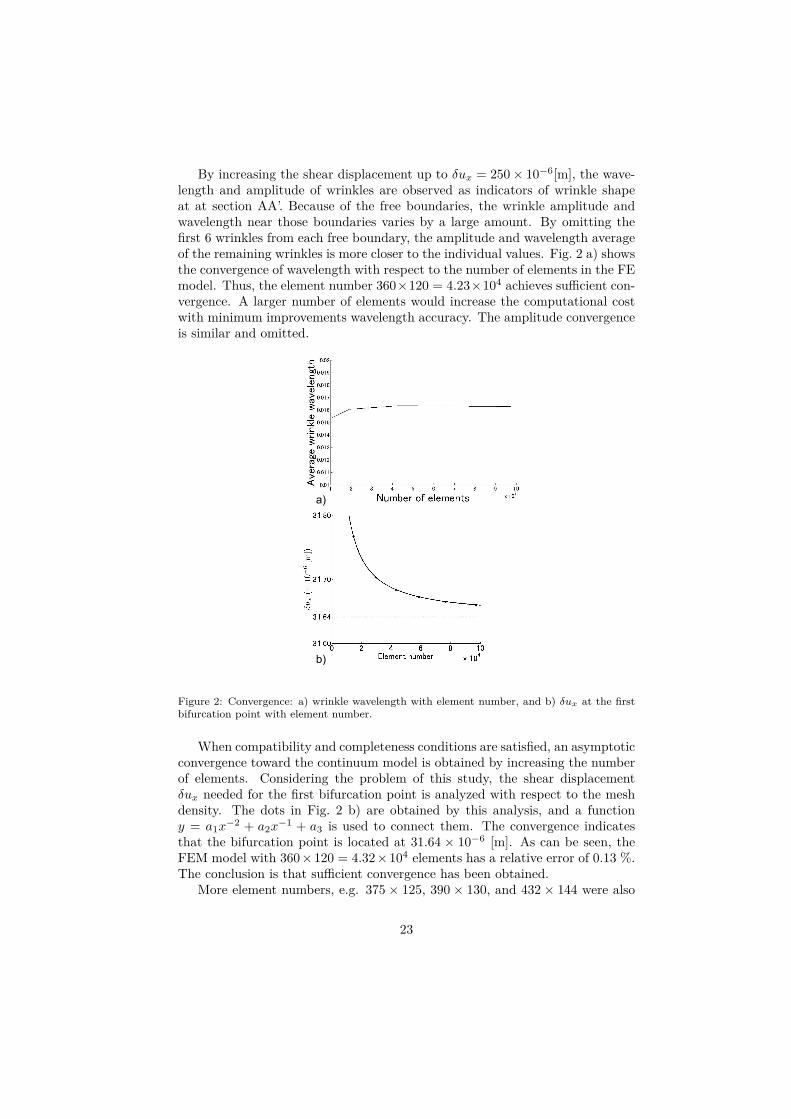
By increasing the shear displacement up to δux = 250 × 10−6[m], the wave-length and amplitude of wrinkles are observed as indicators of wrinkle shapeat at section AA’. Because of the free boundaries, the wrinkle amplitude andwavelength near those boundaries varies by a large amount. By omitting thefirst 6 wrinkles from each free boundary, the amplitude and wavelength averageof the remaining wrinkles is more closer to the individual values. Fig. 2 a) showsthe convergence of wavelength with respect to the number of elements in the FEmodel. Thus, the element number 360×120 = 4.23×104 achieves sufficient con-vergence. A larger number of elements would increase the computational costwith minimum improvements wavelength accuracy. The amplitude convergenceis similar and omitted.

a)

b)

Figure 2: Convergence: a) wrinkle wavelength with element number, and b) δux at the firstbifurcation point with element number.

When compatibility and completeness conditions are satisfied, an asymptoticconvergence toward the continuum model is obtained by increasing the numberof elements. Considering the problem of this study, the shear displacementδux needed for the first bifurcation point is analyzed with respect to the meshdensity. The dots in Fig. 2 b) are obtained by this analysis, and a functiony = a1x−2 + a2x−1 + a3 is used to connect them. The convergence indicatesthat the bifurcation point is located at 31.64 × 10−6 [m]. As can be seen, theFEM model with 360 × 120 = 4.32 × 104 elements has a relative error of 0.13 %.The conclusion is that sufficient convergence has been obtained.

More element numbers, e.g. 375 × 125, 390 × 130, and 432 × 144 were also

23

used for analysis. The results from these numbers of elements were comparedto the result from 360 × 120 elements to confirm that the results convergedand were insensitive above 4.32 × 104 elements. This also applies to results forδux > 250 × 10−6[m].

The convergence of the numerical results is controlled by two additional pa-rameters in the ABAQUS calculation. First, Rα

n is the convergence criterion forthe ratio of the largest residual to the corresponding average flux norm. Thedefault value is Rα

n = 5 × 10−3. Second is Cαn , which is the convergence crite-

rion for the ratio of the largest solution correction to the largest correspondingincremental solution value. Its default value is Cα

n = 1×10−2. For general anal-ysis, the default values are sufficient; however, to obtain more precise results,values that are 10−4 times of the default values are used combined with the δux

increment of 10−7[m].

5.2. 3:1 Free boundary membrane behaviorThe rectangular free boundary membrane is a typical membrane model used

in experiments that focus on membrane wrinkling. The model uses the same ge-ometry and material properties as the 3:1 cyclic boundary membrane defined insection 2. The cyclic boundaries are replaced by free boundaries. The behavioris analyzed using the analysis method described in section 3.4.

5.2.1. Generation of a 34 wrinkle patternThe shear displacement δux is gradually increased for the 0 ≤ δux < 80.48×

10−6 [m] interval. Detail behavior for this interval is given in Senda, et al. [22].Here a summary will be given. At δux = 31.68 × 10−6 [m], the first bifurcationpoint generates 7 wrinkles near each free boundary, resulting in a 14 wrinklepattern. By increasing δux, the number of wrinkles gradually increases. Aftera bifurcation point at δux = 80.48 × 10−6 [m], the membrane is fully wrinkledas shown in Fig. 6 a). Due to free boundaries, the variation in wrinkle shapealong the length of the membrane can be observed.

5.2.2. Collapsed section generationAfter the bifurcation point at δux = 80.48 × 10−6 [m], path tracking is

performed for the interval 80.48 × 10−6 ≤ δux < 440.21 × 10−6[m], as shown inFig. 6. By increasing δux, the wrinkle amplitude decreases locally near the fixedboundaries, resulting in curvature inflections. Further increase in δux results ina section of a wrinkle with out-of-plane displacement of opposite sign than therest of the wrinkle.

Additionally, a shift in collapsed section position is observed. Both am-plitude changes and position shifts occur while all eigenvalues of the tangentstiffness matrix remain positive. Therefore, this behavior occurs without bifur-cations.

Figures 9 and 10 show the first principal stress, σξ and the second principalstress, ση, respectively. The values are observed at δux = 90.00 × 10−6[m].The majority of collapsed sections occur in the region of high tensile σξ and

24

high compressive ση. However, near the free boundaries, both the tension andcompression start to fall off. Therefore, it is difficult to determine in whichregion the collapsed sections originate. By replacing free boundaries with cyclicboundaries, in the later sections it will be shown that the collapsed sectionsoriginate in regions of high tensile σξ and high compressive ση.

5.2.3. Wrinkle generationAt δux = 440.21 × 10−6[m], the collapsed sections of two wrinkles reach

critical sizes. The result is a bifurcation point where one of the two wrinklessplit and two new wrinkles are generated.

In Fig. 7, the behavior at this point can be observed. The initial out-of-plane deformation at δux = 440.21 × 10−6[m], before the disturbance vectorimposition, is observed in Fig. 7 a). The disturbance vector imposition causes asnap through bifurcation. The initial deformation jumps to one of the patternsobserved in Fig. 7 b) and c). The collapsed sections near the top and bottomfixed boundaries of one wrinkle expand toward the middle of the wrinkle. Byincreasing shear to δux = 440.50 × 10−6[m], the generation of new wrinklesis finalized. Figure 7 b) and c) respectively become Fig. 7 d) and e). Theexpanded collapsed sections meet, and the wrinkle amplitude along the centerdrops until it changes its sign. One wrinkle is replaced by three wrinkles, twoof the same sign and one wrinkle of the opposite sign. The collapsed sectionson other wrinkles remain after the bifurcation.

Additional shear increases the size of remaining collapsed sections. The nextbifurcation point is at δux = 645.96 × 10−6[m] where the same process occurs.The out-of-plane deformation at δux = 645.96×10−6[m], before the disturbancevector imposition, is shown in Fig. 8 a). Collapsed sections near the top andbottom fixed boundaries expand toward the middle of the wrinkle as in Fig. 8 b)and c). By slight increase in shear to δux = 646.00 × 10−6[m], Fig. 8 b) and c)respectively, become Fig. 8 d) and e) and the wrinkle generation is completed.

It can be concluded that collapsed sections are the cause of new wrinklegeneration. Essentially, small wrinkles expand and generate larger wrinkles.However, the lack of wrinkle uniformity due to free boundaries makes the obser-vation of collapsed sections inconsistent. As was seen in the results, collapsedsections on wrinkles near the free boundaries have a large variation of shapes.The positioning of collapsed sections is also different from wrinkle to wrinkle.A collapsed section along the middle of a wrinkle may split a wrinkle at smallervalues of shear than a collapsed section that is along the side of a wrinkle.Therefore, additional analysis without effects of free boundaries is needed toclearly explain collapsed section behavior.

5.3. Cyclic boundary membrane behaviorIn the previous section, the behavior where collapsed sections cause wrinkle

generation was shown. This may be a fundamental mechanism to generate newwrinkles when the membrane is fully wrinkled. However, the shape of wrinklesand collapsed sections is affected by the existence of free boundaries. Therefore,

25

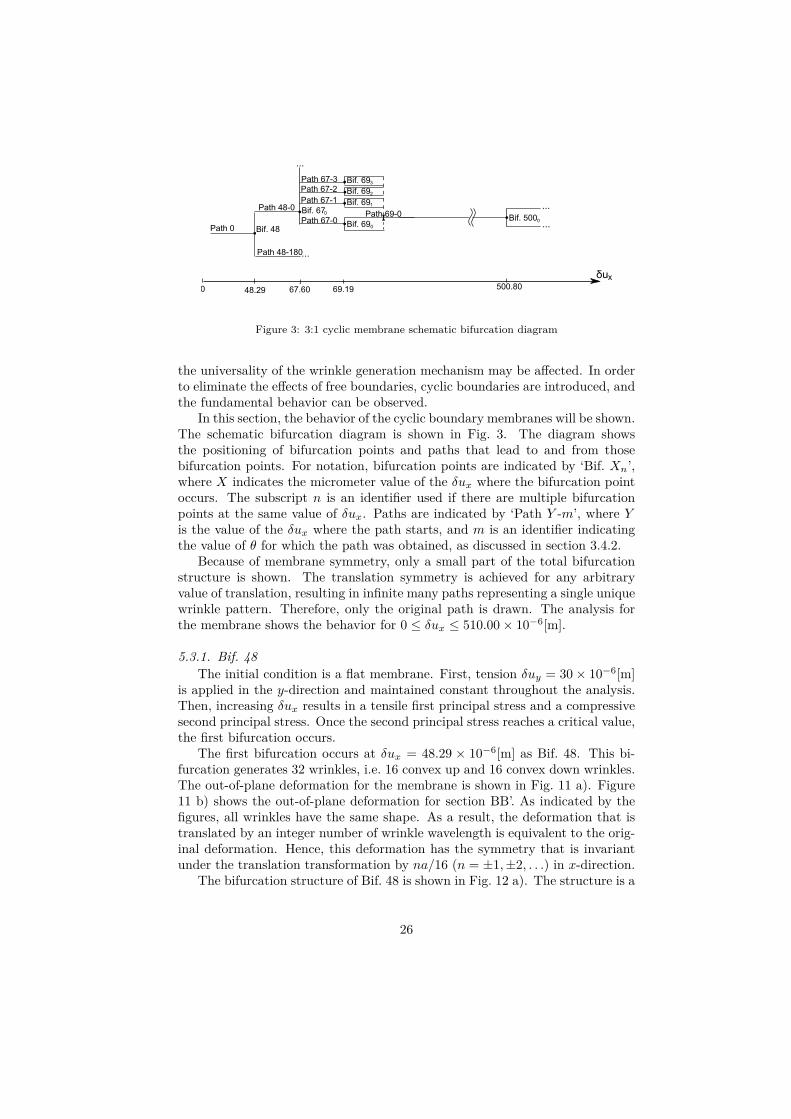
Figure 3: 3:1 cyclic membrane schematic bifurcation diagram

the universality of the wrinkle generation mechanism may be affected. In orderto eliminate the effects of free boundaries, cyclic boundaries are introduced, andthe fundamental behavior can be observed.

In this section, the behavior of the cyclic boundary membranes will be shown.The schematic bifurcation diagram is shown in Fig. 3. The diagram showsthe positioning of bifurcation points and paths that lead to and from thosebifurcation points. For notation, bifurcation points are indicated by ‘Bif. Xn’,where X indicates the micrometer value of the δux where the bifurcation pointoccurs. The subscript n is an identifier used if there are multiple bifurcationpoints at the same value of δux. Paths are indicated by ‘Path Y -m’, where Yis the value of the δux where the path starts, and m is an identifier indicatingthe value of θ for which the path was obtained, as discussed in section 3.4.2.

Because of membrane symmetry, only a small part of the total bifurcationstructure is shown. The translation symmetry is achieved for any arbitraryvalue of translation, resulting in infinite many paths representing a single uniquewrinkle pattern. Therefore, only the original path is drawn. The analysis forthe membrane shows the behavior for 0 ≤ δux ≤ 510.00 × 10−6[m].

5.3.1. Bif. 48The initial condition is a flat membrane. First, tension δuy = 30 × 10−6[m]

is applied in the y-direction and maintained constant throughout the analysis.Then, increasing δux results in a tensile first principal stress and a compressivesecond principal stress. Once the second principal stress reaches a critical value,the first bifurcation occurs.

The first bifurcation occurs at δux = 48.29 × 10−6[m] as Bif. 48. This bi-furcation generates 32 wrinkles, i.e. 16 convex up and 16 convex down wrinkles.The out-of-plane deformation for the membrane is shown in Fig. 11 a). Figure11 b) shows the out-of-plane deformation for section BB’. As indicated by thefigures, all wrinkles have the same shape. As a result, the deformation that istranslated by an integer number of wrinkle wavelength is equivalent to the orig-inal deformation. Hence, this deformation has the symmetry that is invariantunder the translation transformation by na/16 (n = ±1, ±2, . . .) in x-direction.

The bifurcation structure of Bif. 48 is shown in Fig. 12 a). The structure is a

26

symmetric bifurcation. As a result, wrinkles rapidly increase in amplitude froma flat membrane after the bifurcation. The paths are calculated by consideringθ at increments of 30◦. However, a path can be obtained for any θ. Thedisturbance vector is constructed from two orthogonal eigenvectors, and thedisturbance vector of θ = 0◦ is translated in x-direction in accordance with θ.Hence, a path obtained for a certain θ represents a path that is obtained fromthe path of θ = 0◦ by translating in x-direction.

There are Path 48-0 and Path 48-180 after Bif. 48 in Fig. 3 because this isa symmetry bifurcation point. Because the deformation patterns of Path 48-0and Path 48-180 have the reflection symmetry, there is only one wrinkle patternafter Bif. 48. A single path, Path 48-0, defined by θ = 0◦ is tracked by increasingδux.

5.3.2. Bif. 67On Path 48-0, the membrane has 32 wrinkles with same shape. Increasing

δux results in wrinkle amplitude augmentation. The second bifurcation occursat δux = 67.60×10−6[m] as Bif. 670. The out-of-plane deformation of the mem-brane is shown in Fig. 13 a). Figure 13 b) shows the out-of-plane deformation onsection BB’. For Path 48-0, the deformation is a sinusoidal shape with a periodof a/16 in x-direction and a mean of zero. After the bifurcation, a variationof the mean in the form of a sinusoidal deformation with a period of a/2 inx-direction is observed on section BB’. While the variation is observed near thefixed boundaries, it is not observed in the middle of the membrane on sectionAA’.

The bifurcation structure for Bif. 67 is shown in Fig. 12 b). Paths areobtained for values of θ from 0◦ to 360◦ for every 22.5◦. Figure 12 c) showspaths for θ from 0◦ to 22.5◦.

A single group is defined for the θ range of 22.5◦. This is due to the sinusoidaldeformation of period a/2 being imposed onto the base sinusoidal deformationof period a/16. The value of θ defines the x-direction position of the a/2 periodsinusoidal shape. Considering that the full range of imposition of θ is 360◦, theperiod of a/16 in x defines the range of a group as 360◦/16 = 22.5◦.

For a given θ, an equilibrium path will be produced where the peaks of thea/2 period sinusoidal deformation produce two wrinkles with larger amplitudevalues. As indicated by Fig. 3, there are many paths leading form Bif. 670.However, the paths do not exist only for discrete values of θ as the figure sug-gests, but for any arbitrary value. This results in an infinite number of pathsgenerated at Bif. 670. Any two paths in a group have different deformationshapes when their θ values are not same.

By considering a path in group 1 defined as θ = θ′, any group n path definedas θ = θ′ + n × 22.5◦ will have a 5 digit similarity with the group 1 path aftera translation transformation by n a/16. This means that groups represent setsof deformation that are equivalent with translation symmetry. Therefore, onlypaths of one group will be tracked until the next bifurcation.

27

5.3.3. Bif. 69On any Path 67, the membrane has 32 wrinkles where two wrinkles have

slightly larger amplitudes. By increasing δux, the wrinkle amplitude increases.The third bifurcation occurs at δux = 69.19 × 10−6[m] as Bif. 69. This is asymmetric snap through bifurcation. The out-of-plane deformation after thisbifurcation is shown in Fig. 14 a). Figure 14 b) shows the deformation in sectionBB’. The number of wrinkles increases by 2 resulting in a 34 wrinkle pattern. Allwrinkles in this pattern have the same shape. As a result, this deformation hasthe symmetry that is invariant under the translation transformation by na/16(n = ±1, ±2, . . .) in x-direction.

The bifurcation structure for Bif. 69 is shown in Fig. 12 d). As can be seen,there are two paths leading from the bifurcation point. The wrinkle generationoccurs during an unstable split of one of the existing wrinkles. Two wrinklesare candidates for splitting. They correspond to the two wrinkles with slightlylarger amplitudes. Therefore, each of the paths after the bifurcation representone of the wrinkles that splits.

Comparison among all paths generated at Bif. 69, based on all paths of asingle group from Bif. 67, results in 5 digit similarity. Also, the comparisonbetween individual wrinkles for one wrinkle pattern shows that all wrinkles arethe same. Therefore, the conclusion is that after Bif. 69 there exists a singleunique wrinkle pattern but an infinite number of equilibrium paths. All thesepaths correspond to translation transformations in x-direction of the uniquewrinkle pattern. Because of this, only one path is selected for tracking.

5.3.4. Path 69-0Path 69-0 is the selected path after Bif. 69 and it contains 34 wrinkles that

have the same shape. The following behavior observed occurs at regular equi-librium points. The tangent stiffness matrix remains positive definite until thenext bifurcation.

Path 69-0 is observed for 69.19 × 10−6 ≤ δux ≤ 500.80 × 10−6[m]. Byincreasing δux, collapsed sections are generated near the fixed boundaries onexisting wrinkles. Figure 15 b) show the deformation for section BB’ at δux =85.00 × 10−6[m]. The collapsed sections can be observed as a local decrease inwrinkle amplitude near the fixed boundaries.

By increasing δux, these sections grow in size and number. Figures 15 c)and d) show the collapsed section at δux = 500.00 × 10−6[m]. The existence ofthese collapsed sections resulted in all wrinkles having different shapes, wherepreviously all wrinkles were the same shape.

5.3.5. Bif. 500The later part of Path 69-0 is a membrane that contains collapsed section

on existing wrinkles. The fourth bifurcation occurs at δux = 500.80 × 10−6[m]as Bif. 500. The bifurcation is a snap through bifurcation where three wrinklessplit and generate six new wrinkles. The out-of-plane deformation is shown inFig. 16. Figure 16 b) shows the deformation on section BB’. The result of thebifurcation is a 40 wrinkle pattern.

28

The process of wrinkle generation can be observed in Fig. 17. The membranestarts as in Fig. 17 a). The largest collapsed sections are destabilized. A sectionwill rapidly expand along the length of the wrinkle until it meets with theopposite collapsed section in the middle. The affected wrinkles start to split asin Fig. 17 c). The split is then finalized as in Fig. 17 d). The collapsed sectionson the other wrinkles remain.

It can be concluded that after about δux ≈ 80 × 10−6[m], the behavior ofthe cyclic boundary membrane is similar to that of the free boundary mem-brane. Collapsed sections are generated near the fixed boundaries, and as shearis increased, the sections increase in size. At a specific value of shear, theydestabilize the large wrinkle and split it in half. Therefore, it can be concludedthat the free boundaries are not essential in collapsed section formation.

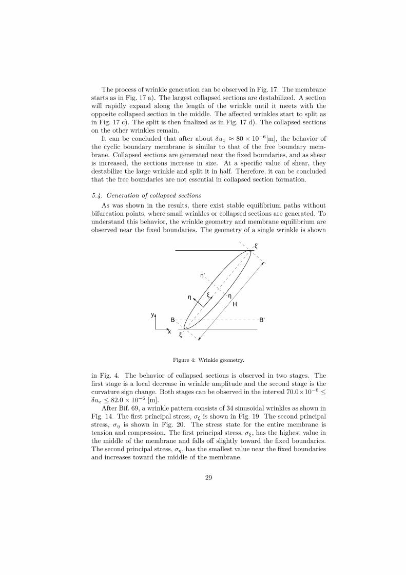
5.4. Generation of collapsed sectionsAs was shown in the results, there exist stable equilibrium paths without

bifurcation points, where small wrinkles or collapsed sections are generated. Tounderstand this behavior, the wrinkle geometry and membrane equilibrium areobserved near the fixed boundaries. The geometry of a single wrinkle is shown

Figure 4: Wrinkle geometry.

in Fig. 4. The behavior of collapsed sections is observed in two stages. Thefirst stage is a local decrease in wrinkle amplitude and the second stage is thecurvature sign change. Both stages can be observed in the interval 70.0×10−6 ≤δux ≤ 82.0 × 10−6 [m].

After Bif. 69, a wrinkle pattern consists of 34 sinusoidal wrinkles as shown inFig. 14. The first principal stress, σξ is shown in Fig. 19. The second principalstress, ση is shown in Fig. 20. The stress state for the entire membrane istension and compression. The first principal stress, σξ, has the highest value inthe middle of the membrane and falls off slightly toward the fixed boundaries.The second principal stress, ση, has the smallest value near the fixed boundariesand increases toward the middle of the membrane.

29

First the interval 70.0 × 10−6 ≤ δux ≤ 74.0 × 10−6 [m] is observed onsections ξξ′ and ηη′. Definition of the sections ξξ′ and ηη′ is shown in Fig. 18.The position on the section is defined by node values based on the finite elementnodes. Figures 21 and 22 show the principal stress values on section ξξ′. As δux

is increased, the first principal stress increases for the entire section. The secondprincipal stress decreases, however the change is small compared the total value.

Figure 23 shows the out-of-plane displacement, uz, on section ξξ′. Figure24 shows the curvature, ∂2uz/∂ξ2 = κη, on section ξξ′. Figure 25 shows theout-of-plane displacement, uz, on section ηη′. Figure 26 shows the curvature,∂2uz/∂η2 = κξ, on section ηη′. The sections cross each other at node 15 ofsection ξξ′, and node 9 of section ηη′. For the interval 70.0 × 10−6 ≤ δux ≤72.0×10−6 [m], the increasing δux increases the wrinkle amplitude for the entiresection. At δux = 73.0 × 10−6 [m], a drop in amplitude is observed betweennodes 1 and 32, while an increase is observed after node 32. The curvatureκξ in Fig. 26 shows that while the amplitude decreases, the wrinkle maintainsa convex up shape along η. The curvature κη in Fig. 24 is positive betweennodes 1 and 7, and increases for interval 70.0 × 10−6 ≤ δux ≤ 72.0 × 10−6 [m].However, for δux = 73.0 × 10−6 [m] it starts dropping. For nodes after node 7,the curvature κη is negative with a minimum value at node 11. For the interval70.0 × 10−6 ≤ δux ≤ 72.0 × 10−6 [m], the minimum value decreases. However,it increases for δux = 73.0 × 10−6 [m].

Next, the interval 74.0 × 10−6 ≤ δux ≤ 82.0 × 10−6 [m] is observed. Theprincipal stress behavior is the same as before; both tension and compressionincrease. Figure 29 shows the out-of-plane displacement, uz, on section ξξ′.Figure 30 shows the curvature, κη, on section ξξ′. Figure 31 shows the out-of-plane displacement, uz, on section ηη′. Figure 32 shows the curvature, κξ, onsection ηη′. As δux increases, amplitude up to node 32 continues decreasing.As a result, the curvature, κη, also approaches 0. At δux = 76.0 × 10−6 [m],the decrease in wrinkle amplitude reached the point where the wrinkle becomesflat in the η-direction as seen in Figs. 31 and 32. At the flat top of the wrinkle,it can be observed that both κη and κξ are almost 0. The amplitude dropsfurther and a convex up wrinkle gains a convex down peak. At this point bothcurvature κη and κξ change their signs.

Following the discussion about thin plate bending in Timoshenko[3], theequilibrium of a plate element in z-direction can be written as

∂Qξ

∂ξ+ ∂Qη

∂η= Nξκη + Nηκξ (74)

The left side of the above expression represents the bending of the plate dueto transversal forces Q, while the right side represents the membrane behaviordue to mid-plane forces N . The mid-plane forces Nξ and Nη are obtained byintegration of principal stress values over the membrane thickness. The valuescan be approximated as Nξ = hσξ and Nη = hση where h is the membranethickness. The transversal forces are obtained in Fig. 33 as Qξ and in Fig. 34as Qη. At the fixed boundary, the transversal forces correspond to the reaction

30

forces from the boundary. By moving away from the fixed boundary, both Qξ

and Qη increase rapidly toward 0. After node 8 of the ξξ′ section and node11 of the ηη′ section the values become almost constant. By observing theequilibrium equation, it can be concluded that very near the fixed boundaries,the membrane behavior is determined by both transversal and mid-plane forces.In other words, the membrane behaves as a thin plate. By moving away fromthe fixed boundaries, the effects of transversal forces fall off and the behavior ismostly determined by mid-plane forces. Therefore, the left side of Eq. (74) isapproximately zero, and the equation becomes a membrane equilibrium.

Near the the fixed boundaries, positive σξ over positive κη results in anupward force. The negative ση over negative κξ also results in an upward force.The equilibrium is maintained by the downward transversal forces near thefixed boundaries, due to the bending stiffness of the membrane. Because of thebending stiffness and the boundary conditions, κη is positive and out-of-planedisplacement is inhibited.

When a flat membrane is considered, positive σξ and negative ση corre-spond to the extension of membrane length along ξ-direction and the reductionof membrane length along η-direction. In addition, σξ and ση are generally pro-portional to δux and constant throughout the membrane. However, in the actualmembrane, out-of-plane deformation has occurred, which results in Figs. 19 to26.

As shown in Figs. 19 and 21, there is only a small percentage differencein σξ between the values in the middle of the membrane and near the fixedboundaries. As δux is increased, the length of the membrane along ξ-directionincreases, resulting in higher values of σξ.

As shown in Figs. 20 and 22, there is an order of one difference in ση mag-nitude between the values in the middle of the membrane and near the fixedboundaries. After node 20, with increasing δux there is no significant change inση, meaning there is no significant reduction in membrane length. As indicatedby Fig. 23, the reduction in length along η-direction does not occur becausethe wrinkle amplitude is increased which releases the stress. However, by ap-proaching the fixed boundaries, the increase in δux results in an increase incompression, meaning there exists a reduction in length along the η-direction.This is because the fixed boundaries limit the increase in amplitude and preventthe release of stress.

Additional increase in δux is shown in Figs. 27 to 32. With the increasein δux, the length of the membrane along ξ-direction continues to increase asindicated by σξ in Fig. 27. As for ση, in contrast to Fig. 22, for nodes 9–20there is almost no change in ση as shown in Fig. 28. This means that there isno reduction in membrane length along η-direction for these nodes. In addition,Fig. 29 shows a decrease in wrinkle amplitude for the same nodes. However,along η-direction, there is an increase in wrinkle number, as shown in Fig. 31.By increasing the wrinkle number, the stress in the membrane is released andthe reduction in length along the η-direction is avoided. This increase in wrinklenumber is represented by collapsed sections.

From the presented behavior, it can be concluded that the generation of

31

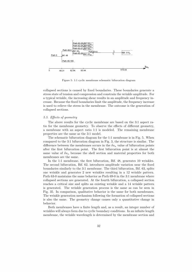
Figure 5: 1:1 cyclic membrane schematic bifurcation diagram

collapsed sections is caused by fixed boundaries. These boundaries generate astress state of tension and compression and constrain the wrinkle amplitude. Fora typical wrinkle, the increasing shear results in an amplitude and frequency in-crease. Because the fixed boundaries limit the amplitude, the frequency increaseis used to relieve the stress in the membrane. The outcome is the generation ofcollapsed sections.

5.5. Effects of geometryThe above results for the cyclic membrane are based on the 3:1 aspect ra-

tio for the membrane geometry. To observe the effects of different geometry,a membrane with an aspect ratio 1:1 is modeled. The remaining membraneproperties are the same as the 3:1 model.

The schematic bifurcation diagram for the 1:1 membrane is in Fig. 5. Whencompared to the 3:1 bifurcation diagram in Fig. 3, the structure is similar. Thedifference between the membranes occurs in the δux value of bifurcation pointsafter the first bifurcation point. The first bifurcation point is at almost thesame value of δux because the shell section and material properties for bothmembranes are the same.

In the 1:1 membrane, the first bifurcation, Bif. 48, generates 10 wrinkles.The second bifurcation, Bif. 62, introduces amplitude variation near the fixedboundaries similarly to the 3:1 membrane. The third bifurcation, Bif. 63, splitsone wrinkle and generates 2 new wrinkles resulting in a 12 wrinkle pattern.Path 63-0 maintains the same behavior as Path 69-0 in the 3:1 membrane wherecollapsed sections are generated. At the fourth bifurcation, a collapsed sectionreaches a critical size and splits an existing wrinkle and a 14 wrinkle patternis generated. The wrinkle generation process is the same as can be seen inFig. 35. In comparison, qualitative behavior is the same for both membranes.The wrinkle generation mechanism following the formation of collapsed sectionsis also the same. The geometry change causes only a quantitative change inbehavior.

Both membranes have a finite length and, as a result, an integer number ofwrinkles will always form due to cyclic boundary conditions. In an infinite lengthmembrane, the wrinkle wavelength is determined by the membrane section and

32

material properties and loads. In a fixed length membrane with cyclic boundaryconditions, the wrinkle wave length will round up/down to a value that resultsin an integer value of wrinkles. The effect of wrinkle wavelength is membranestability. As can be observed by the results, the more wrinkles are present, thesmaller the wrinkle wavelength and a larger value of δux needed for a bifurcationpoint. Therefore, the difference in wrinkle wavelength between the 3:1 and 1:1membranes can explain the variations in δux values of bifurcation points.

6. Conclusion

In this study, the equilibrium path tracking method with the finite elementmethod is used to obtain the wrinkling behavior of rectangular membranes un-dergoing shear displacement. Initially, a membrane with free boundaries andaspect ratio of 3:1 is analyzed. For this membrane model, by increasing the sheardisplacement, the entire membrane becomes wrinkled. However, the presenceof free boundaries results in an uneven shape and distribution of the wrinkles.By further increase in shear, small wrinkles referred to as collapsed sections aregenerated on existing wrinkles near fixed boundaries. These sections increasein size and generate new wrinkles. However, the universality of this wrinklegeneration behavior may be affected by free boundaries. Therefore, the ef-fect of free boundaries is removed by replacing the free boundaries with cyclicboundaries. By removing the free boundaries and observing the generation ofcollapsed sections, it is concluded that the cause of collapsed sections are thefixed boundaries. Because fixed boundaries constrain the amplitude of a wrinkle,the additional deformation energy form increasing shear results in an increasedwrinkle frequency near the boundary. This increased frequency is representedby collapsed sections. Because fixed boundaries are common in membrane struc-tures, understanding how these boundaries generate new wrinkles is useful inpredicting the structure behavior.

7. Vitae

Kei SendaKei Senda received the Ph. D. in engineering in 1993 from Osaka Prefecture

University. From 1988 to 2008, he worked for Osaka Prefecture University andKanazawa University. From 2008, has been a professor of Department of Aero-nautics and Astronautics, Graduate School of Engineering, Kyoto University.His research activities have included more than 100 papers on the dynamicsand control of aerospace systems, the intelligence and autonomy for mechanicalsystems, and the motion intelligence of animals. He received the Best PresentedPaper Award of the AIAA Guidance, Navigation, and Control Conference in1992, etc.

33

Mario PetrovicMario Petrovic, obtained a bachelor degree in 2008 at the University of

Zagreb, Faculty of mechanical engineering and naval architecture, on the topicof numerical simulation of rigid body mechanisms. In 2010, graduated from theUniversity with a master degree on the topic of numerical simulation of dynamicand fatigue in wind turbines. Current position is a doctor course student atKyoto University, Graduate school of engineering. Here, he conducts researchinto inflatable structures, where the focus is on the generation of wrinkles in amembrane in an attempt to predict membrane behavior.

Kei NakanishiKei Nakanishi obtained both Bachelor degree in 2010 and Master degree

in 2012 from Kyoto University. Their topic is numerical analysis of shearedrectangular membrane in inflatable space structures.

References

[1] A.B. Chmielewsk, Overview of Gossamer Structures in: C.H.M. Jenkins(Eds.), Gossamer Spacecraft: Membrane and Inflatable Structures Tech-nology for Space Applications, AIAA, Reston, VA, 2001, pp.1-20.

[2] K. Senda, T. Oda, S. Ota, Y. Igarashi, A. Watanabe, T. Hori, H. Ito,H. Tsunoda, K. Watanabe, Deploy Experiment of Inflatable Tube usingWork Hardening, Proc. AIAA Gossamer Spacecr. Forum, AIAA-2006-1808(2006) 1-18.

[3] S.P. Timoshenko, J.M. Gere, Theory of Elastic Stability, second ed.,Springer, New York, 2010.

[4] Y.W. Wong, S. Pellegrino, Wrinkled Membranes, Part I, J. of Mechanicsof Mater. Structures, Vol. 1, No. 1 (2006) 3-25.

[5] Y.W. Wong, S. Pellegrino, Wrinkled Membranes, Part II, J. of Mechanicsof Mater. Structures, Vol. 1, No. 1 (2006) 27-61.

[6] Y.W. Wong, S. Pellegrino, Wrinkled Membranes, Part III, J. of Mechanicsof Mater. Structures, Vol. 1, No. 1 (2006) 63–95.

[7] R.K. Miller, J.M. Hedgepeth, An Algorithm for Finite Element Analysis ofPartly Wrinkled Membranes, AIAA J., Vol. 20, No. 12 (1982) 1761-1763.

[8] R.K. Miller, J.M. Hedgepeth, V.I. Weingarten, P. Das, S. Kahyai, FiniteElement Analysis of Partly Wrinkled Membranes, Computers & Structures,Vol. 20, Nos. 1-3 (1985) 631-639.

[9] Y. Miyazaki, Wrinkle/Slack Model and Finite Element Dynamics of Mem-brane, International J. for Numerical Methods in Engineering, Vol. 66,No. 7 (2006) 1179-1209.

34

[10] Z.P. Bazant, L. Cedelon, Stability of Structures, Oxford University Press,New York, 1991.

[11] C.G. Wang, X.W. Du, H.F. Tan, X.D. He, A New Computational Methodfor Wrinkling Analysis of Gossamer Space Structures, International J. ofSolids and Structures, Vol. 46, No. 6 (2009) 1516-1526

[12] A. Tessler, D.W. Sleight, J.T. Wang, Effective Modeling and NonlinearShell Analysis of Thin Membranes Exhibiting Structural Wrinkling, J. ofSpacecr. Rockets, Vol. 42, No. 2 (2005) 287-298.

[13] P. Wiggers, W. Wanger, C. Miehe, A quadratically convergent procedurefor the calculation of stability points in finite element analysis, ComputerMethods in Appl. Mechanics and Engineering, Vol. 70, No. 3 (1988) 329-347.

[14] J. Leifer, D.C. Jones, A.M. Cook, Gravity-Induced Wrinkling in Subscale,Singly Curved Parabolic Gossamer Membrane, J. of Spacecr. Rockets, Vol.47, No. 1 (2010) 214-219.

[15] K. Woo, C.H. Jenkins, Effect of Crease Orientation on Wrinkle-CreaseInteraction for Thin Membranes, J. of Spacecr. Rockets, Vol. 50, No. 5(2013) 1024-1034.

[16] A. Tessler, D.W. Sleight, Geometrically Nonlinear Shell Analysis of Wrin-kled Thin-Film Membranes with Stress Concentrations, J. of Spacecr.Rockets, Vol. 44, No. 3 (2007) 582-588.

[17] S. Inoue,Prediction Methods of Wrinkling in Thin-Membrane, Proc. of In-ternational Symposium on Space Technology and Science, Tsukuba, Japan,(2009) 1-7.

[18] A. Endo, Y. Hangai, S. Kawamata, Post-Buckling Analysis of Elastic Shellsof Revolution by the Finite Element Method, Rep. of Inst. of IndustrialScience, 624.074.4:624.075.4 (1976).

[19] P. Wriggers, W. Wanger, C. Miehe, A Quadratically Convergent Proce-dure for the Calculation of Stability Points in Finite Element Analysis,Computer Methods in Appl. Mechanics and Engineering, Vol. 70, No. 3(1988) 329-347.

[20] R. Hoyle, Pattern Formation, Cambridge University Press, New York, 2007.

[21] B.S. Reddy, B. N. Chatterji, An FFT-based technique for translation, rota-tion, and scale-invariant image registration,’ IEEE Transactions on ImageProcessing 5, Vol. 5, No. 8 (1996) 1266-1271.

[22] K. Senda, K. Nakanishi, K. Takagi, Wrinkle Generation Mechanism with-out Buckling in Sheared Rectangular Membrane, Proc. AIAA GossamerSpacecr. Forum, AIAA-2012-1919 (2012).

35

34 wrinkle pattern

generation of collapsed sections

expansion of collapsed sections

after unstable expansion of a collapsed section = 36 wrinkles

a)

b)

c)

d)Figure 6: Wrinkle pattern progression, free boundary membrane: a) δux = 80.48 × 10−6[m];b) δux = 90.00 × 10−6[m]; c) δux = 440.00 × 10−6[m]; d) δux = 440.21 × 10−6[m].

36

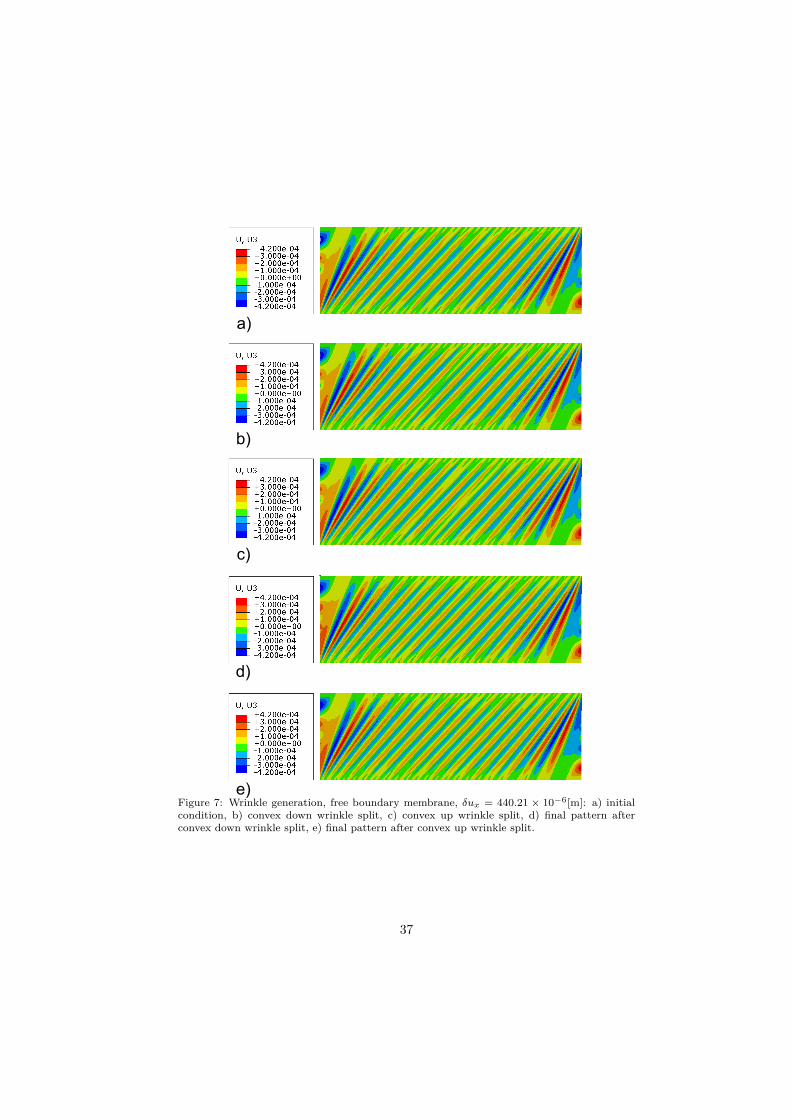
a)

b)

c)

d)

e)Figure 7: Wrinkle generation, free boundary membrane, δux = 440.21 × 10−6[m]: a) initialcondition, b) convex down wrinkle split, c) convex up wrinkle split, d) final pattern afterconvex down wrinkle split, e) final pattern after convex up wrinkle split.

37

a)

b)

c)

d)

e)Figure 8: Wrinkle generation, free boundary membrane, δux = 645.96 × 10−6[m]: a) initialcondition, b) convex down wrinkle split, c) convex up wrinkle split, d) final pattern afterconvex down wrinkle split, e) final pattern after convex up wrinkle split.

38

Figure 9: First principal stress, σξ, freeboundary membrane.

Figure 10: Second principal stress, ση , freeboundary membrane.

Figure 11: Out-of-plane deformation after Bif. 48, cyclic boundary membrane.

39

Figure 12: Bifurcation diagrams for cyclic membrane; a) Bif. 48, b) Bif. 67, c) close up afterBif. 67, d) Bif. 69.

Figure 13: Out-of-plane deformation after Bif. 67, cyclic boundary membrane.

40

Figure 14: Out-of-plane deformation after Bif. 69, cyclic boundary membrane.

Figure 15: Out-of-plane deformation on Path 69-0, cyclic boundary membrane.

41

Figure 16: Out-of-plane deformation, Bif. 500, cyclic boundary membrane.

Figure 17: Wrinkle split, Bif. 500, cyclic boundary membrane: a) initial condition, b) start ofrapid collapsed section expansion, c) wrinkle splitting, d) final wrinkle pattern.

42

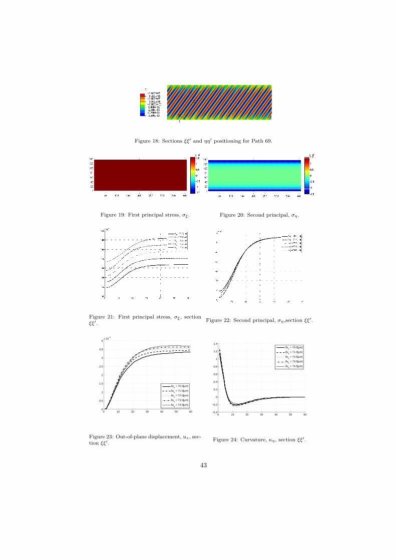
Figure 18: Sections ξξ′ and ηη′ positioning for Path 69.

Figure 19: First principal stress, σξ. Figure 20: Second principal, ση .

Figure 21: First principal stress, σξ, sectionξξ′. Figure 22: Second principal, ση ,section ξξ′.

0 10 20 30 40 50 600

0.5

1

1.5

2

2.5

3

3.5

4x 10

−5

δux = 70.0[µm]

δux = 71.0[µm]

δux = 72.0[µm]

δux = 73.0[µm]

δux = 74.0[µm]

Figure 23: Out-of-plane displacement, uz , sec-tion ξξ′.

0 10 20 30 40 50 60−0.4

−0.2

0

0.2

0.4

0.6

0.8

1

1.2

1.4

δu

x = 70.0[µm]

δux = 71.0[µm]

δux = 72.0[µm]

δux = 73.0[µm]

δux = 74.0[µm]

Figure 24: Curvature, κη , section ξξ′.

43

0 2 4 6 8 10 12 14 16−4

−3

−2

−1

0

1

2

3x 10

−5

δux = 70.0[µm]

δux = 71.0[µm]

δux = 72.0[µm]

δux = 73.0[µm]

δux = 74.0[µm]

Figure 25: Out-of-plane displacement, uz , sec-tion ηη′.

0 2 4 6 8 10 12 14 16−8

−6

−4

−2

0

2

4

6

8

10

δu

x = 70.0[µm]

δux = 71.0[µm]

δux = 72.0[µm]

δux = 73.0[µm]

δux = 74.0[µm]

Figure 26: Curvature, κξ, section ηη′.

0 10 20 30 40 50 601.58

1.6

1.62

1.64

1.66

1.68

1.7

1.72

1.74

1.76x 10

6

δu

x = 74.0[µm]

δux = 76.0[µm]

δux = 78.0[µm]

δux = 80.0[µm]

δux = 82.0[µm]

Figure 27: First principal stress, σξ, sectionξξ′.

0 10 20 30 40 50 60−16

−14

−12

−10

−8

−6

−4

−2

0x 10

4

δux = 74.0[µm]

δux = 76.0[µm]

δux = 78.0[µm]

δux = 80.0[µm]

δux = 82.0[µm]

Figure 28: Second principal, ση ,section ξξ′.

0 10 20 30 40 50 600

0.5

1

1.5

2

2.5

3

3.5

4

4.5x 10

−5

δux = 74.0[µm]

δux = 76.0[µm]

δux = 78.0[µm]

δux = 80.0[µm]

δux = 82.0[µm]

Figure 29: Out-of-plane displacement, uz , sec-tion ξξ′.

0 10 20 30 40 50 60−0.2

0

0.2

0.4

0.6

0.8

1

1.2

δu

x = 74.0[µm]

δux = 76.0[µm]

δux = 78.0[µm]

δux = 80.0[µm]

δux = 82.0[µm]

Figure 30: Curvature, κη , section ξξ′.

44

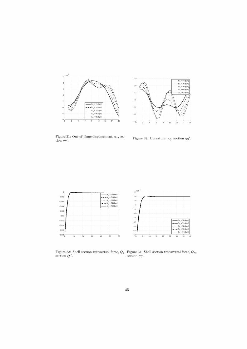
0 2 4 6 8 10 12 14 16−4

−3

−2

−1

0

1

2

3x 10

−5

δux = 74.0[µm]

δux = 76.0[µm]

δux = 78.0[µm]

δux = 80.0[µm]

δux = 82.0[µm]

Figure 31: Out-of-plane displacement, uz , sec-tion ηη′.

0 2 4 6 8 10 12 14 16−15

−10

−5

0

5

10

15

δu

x = 74.0[µm]

δux = 76.0[µm]

δux = 78.0[µm]

δux = 80.0[µm]

δux = 82.0[µm]

Figure 32: Curvature, κξ, section ηη′.

0 10 20 30 40 50 60−0.018

−0.016

−0.014

−0.012

−0.01

−0.008

−0.006

−0.004

−0.002

0

δu

x = 70.0[µm]

δux = 71.0[µm]

δux = 72.0[µm]

δux = 73.0[µm]

δux = 74.0[µm]

Figure 33: Shell section transversal force, Qξ,section ξξ′.

0 5 10 15 20 25 30 35 40−18

−16

−14

−12

−10

−8

−6

−4

−2

0

2x 10

−3

δux = 70.0[µm]

δux = 71.0[µm]

δux = 72.0[µm]

δux = 73.0[µm]

δux = 74.0[µm]

Figure 34: Shell section transversal force, Qη ,section ηη′.

45

Figure 35: Wrinkle split, Bif. 515, 1:1 cyclic boundary membrane: a) initial condition, b) startof rapid collapsed section expansion, c) wrinkle splitting, d) final wrinkle pattern.

Figure 36: Author: Kei Senda

46

Figure 37: Author: Mario Petrovic

Figure 38: Author: Kei Nakanishi (placeholder)

47