Embed Size (px)
Citation preview

Numerical Studies for theRasch Model with Many ItemsHelmut Strasser
Research Report Series Institute for Statistics and MathematicsReport 119, Marz 2012 http://statmath.wu.ac.at/
Numerical studies for the Rasch model with manyitems
Helmut Strasser
March 12, 2012
Abstract
This paper is concerned with numerical studies on the theoretical results obtainedin Strasser [1] and [2]. These papers provide asymptotic expansions for conditionalexpectations of non i.i.d. Bernoulli trials and their application to the covariancestructure of conditional maximum likelihood estimates for the Rasch model.
In the present paper systematic numerical studies of the accuracy of the approx-imations given in Strasser [1] and [2] are presented. It is shown that the order ofapproximation claimed by the theoretical results can be established numerically.
Contents1 Introduction 2
2 Exact calculation of conditional moments 2
3 Approximation of conditional moments 6
4 Conditional m.l. estmation for the Rasch model 12
5 Exact calculations for the Rasch model 14
6 Approximations for the Rasch model 146.1 The Fisher information . . . . . . . . . . . . . . . . . . . . . . . . . . . 146.2 The asymptotic covariance matrix . . . . . . . . . . . . . . . . . . . . . 17
7 Appendix: R-Code 19
1
1 INTRODUCTION 2
1 Introduction
For an introduction into the problem we refer to the introductory sections of the papersby Strasser, [1] and [2]. The numerical studies in the present paper are coded in the S-language. The algorithms can be carried out by the software R. In the appendix of thispaper (section 7) we collect some R-code of basic algorithms.
2 Exact calculation of conditional moments
Let X1, X2, . . . , Xn independent random variables with values 0 and 1 and probabilitiesP (Xi = 1) = pi. Let Sn := X1 +X2 +· · ·+Xn be their sum. The main results of Strasser[1] are asymptotic expansions being valid as n → ∞ for the conditional expectationsE(Xi|Sn) and E(XiXj|Sn) as well as for the expectations of the conditional covariances.
The elementary symmetric polynomial of order s of a vector x = (x1, . . . , xn) is definedby
γns :=∑{ n∏
i=1
xyii :n∑i=1
yi = s, yi ∈ N0
}It is convenient to calculate these polynomials by an algorithm that is similar to Pascal’striangle for binomial coefficients. For elementary symmetric polynomials this algorithmruns as follows:
γk0 = 1 whenever k ≥ 0,
γkr = xkγk−1,r−1 + γk−1,r if k ≥ 1 and 1 ≤ r ≤ k, (1)γkr = 0, if r > k.
The values of the elementary symmetric polynomials increase with n and quickly attainhuge values, similarly as binomial coefficients do. For numerical purposes it is thereforepreferable to normalize the values of the elementary symmetric polynomials somehow.
There is a relation between elementary symmetric polynomials and certain probabilitieswhich extends the familiar relation between binomial coefficients and binomial probabil-ities. We have
P (Sn = s) =∑
y:∑yi=s
∏i
pyii (1− pi)1−yi =γns
(1 + xi)n,
where xi = pi/(1 − pi). It is numerically more efficient to calculate these probabilitesinstead of the elementary symmetric polynomials. It is straightforward to extend thealgorithm (1) to the calculation of those probabilities. This algorithm is coded by theR-function (see section 7)
2 EXACT CALCULATION OF CONDITIONAL MOMENTS 3
prob <− f u n c t i o n ( p , d rop =TRUE)
which returns the values of all probabilities P (Sn = s), s = 0, 1, . . . , n, for a givenvector p = (pi) of probabilities. Note that for vectors p with equal components binomialprobabilities are obtained.
2.1 EXAMPLE.
> prob ( r e p ( 0 . 3 , 1 0 ) )[ 1 ] 0 .0282475249 0.1210608210 0.2334744405 . . .
> prob ( ( 1 : 9 ) / 1 0 )[ 1 ] 0 .00036288 0 .00699984 0 .04820760 0 .15974936 . . .
After these preparations it is easy to calculate conditional expectations. Let
Sin−1 :=∑k 6=i
Xk, Sijn−2 :=∑k 6=i,j
Xk
Then we have
E(Xi|Sn = s) =P (Xi = 1, Sn = s)
P (Sn = s)= pi
P (Sin−1 = s− 1)
P (Sn = s)(2)
E(XiXj|Sn = s) =P (Xi = 1, Xj = 1, Sn = s)
P (Sn = s)= pipj
P (Sijn−2 = s− 2)
P (Sn = s), i 6= j. (3)
These formulas are coded by the R-function (see section 7)
cm_exact <− f u n c t i o n ( p , i =1 , j =NULL)
where p is a vector of probabilities. The function returns vectors as(i) = E(Xi|Sn = s)and bs(i, j) = E(XiXj|Sn = s). Note that for vectors p with equal components there areexplicit expressions for the conditional moments:
as(i) = E(Xi|Sn = s) =s
n
bs(i, j) = E(XiXj|Sn = s) =s(s− 1)
n(n− 1), i 6= j.
2.2 EXAMPLE.
> cm_exact ( r e p ( 0 . 1 , 5 ) , 1 )[ 1 ] 0 . 0 0 . 2 0 . 4 0 . 6 0 . 8 1 . 0
> cm_exact ( r e p ( 0 . 1 , 5 ) , 1 , 2 )
2 EXACT CALCULATION OF CONDITIONAL MOMENTS 4
[ 1 ] 0 . 0 0 . 0 0 . 1 0 . 3 0 . 6 1 . 0
> cm_exact ( r u n i f ( 5 ) , 1 )[ 1 ] 0 .0000000 0 .2049964 0 .4767453 0 .7231139 0 .9178962 . . .
> cm_exact ( r u n i f ( 5 ) , 1 , 2 )[ 1 ] 0 .00000000 0 .00000000 0 .04486523 0 .21934904 0 .65105522[ 6 ] 1 .00000000
Next we would like to calculate the conditional covariance matrix
Fns := E(XXt|Sn = s)− E(X|Sn = s)E(X|Sn = s)t (4)
and the expectation of the conditional covariance matrix
Fn := E(E(XXt|Sn)− E(X|Sn)E(X|Sn)t
)=
n∑s=0
FnsP (Sn = s) (5)
These evaluations are obviously based on the previous calculations. They are coded bythe R-functions (see section 7)
v c o n d _ e x a c t <− f u n c t i o n ( p )v _ e x a c t <− f u n c t i o n ( p )
The function vcond_exact simply collects the results of cm_exact and puts theminto an array cijs = (Fns)ij according to (4). The function v_exact evaluates (5) andreturns the matrix Fn.
It should be noted that the evaluation of these matrices for large n needs computing time.
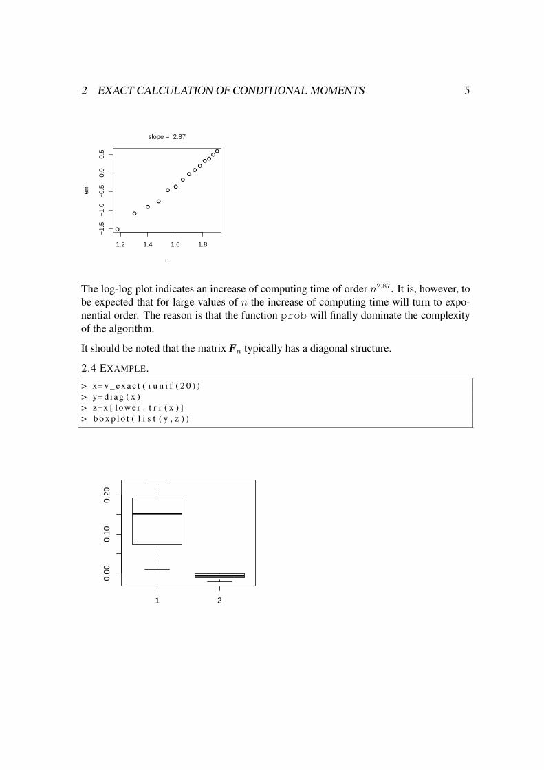
2.3 EXAMPLE. Let us carry out a computer experiment concerning the calculation timeof Fn for increasing n. The R-function errplot (see section 7) draws a log-log plot andcalculates the slope of the regression line.
> p= r u n i f ( 5 0 )> tm= numer ic ( 0 )> nn= seq ( 1 0 , 8 0 , by =5)> f o r ( n i n nn ) tm=c ( tm , sys tem . t ime ( v _ e x a c t ( r u n i f ( n ) ) ) [ 1 ] )> e r r p l o t ( nn [−1] , tm [−1])
2 EXACT CALCULATION OF CONDITIONAL MOMENTS 5
●
●
●
●
●●
●
●●
●
●●
●●
1.2 1.4 1.6 1.8
−1.
5−
1.0
−0.
50.
00.
5
n
err
slope = 2.87
The log-log plot indicates an increase of computing time of order n2.87. It is, however, tobe expected that for large values of n the increase of computing time will turn to expo-nential order. The reason is that the function prob will finally dominate the complexityof the algorithm.
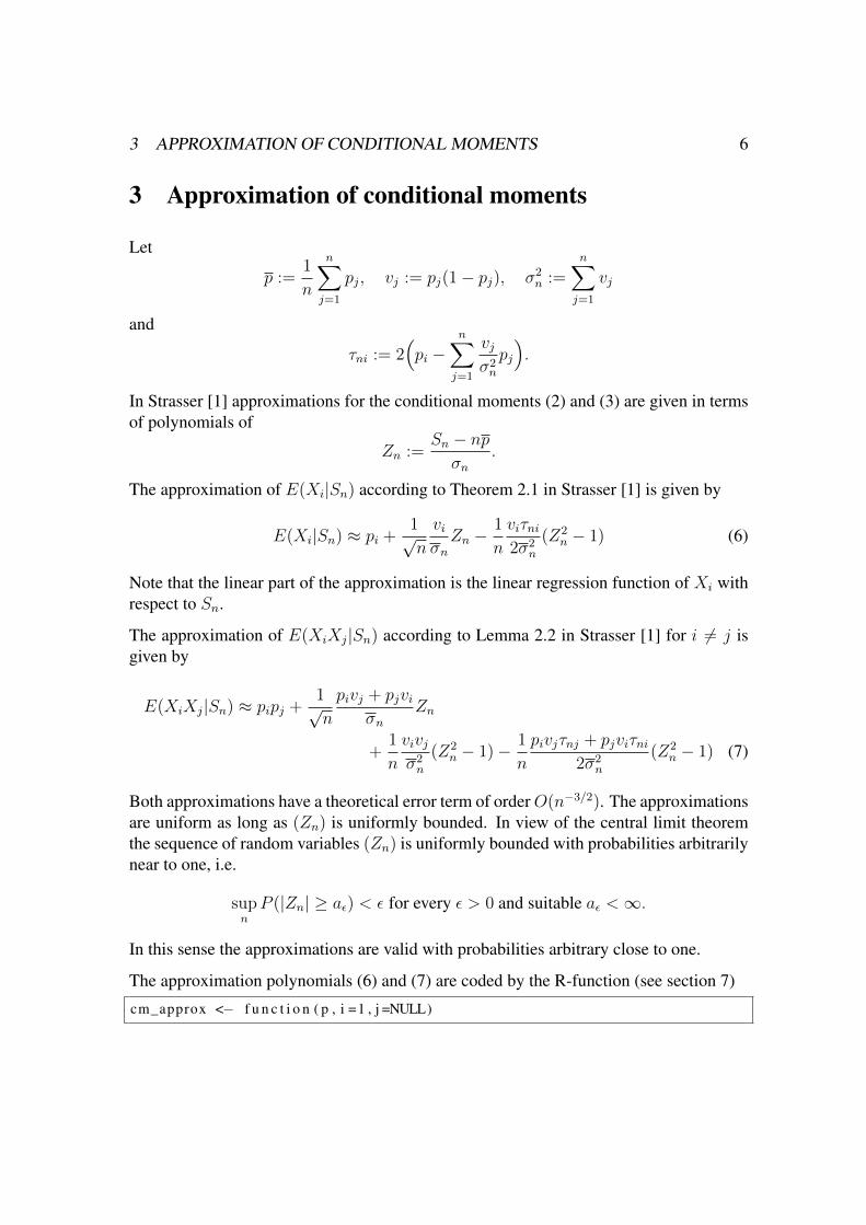
It should be noted that the matrix Fn typically has a diagonal structure.
2.4 EXAMPLE.
> x= v _ e x a c t ( r u n i f ( 2 0 ) )> y= d i a g ( x )> z=x [ lower . t r i ( x ) ]> b o x p l o t ( l i s t ( y , z ) )
1 2
0.00
0.10
0.20
3 APPROXIMATION OF CONDITIONAL MOMENTS 6
3 Approximation of conditional moments
Let
p :=1
n
n∑j=1
pj, vj := pj(1− pj), σ2n :=
n∑j=1
vj
and
τni := 2(pi −
n∑j=1
vjσ2n
pj
).
In Strasser [1] approximations for the conditional moments (2) and (3) are given in termsof polynomials of
Zn :=Sn − npσn
.
The approximation of E(Xi|Sn) according to Theorem 2.1 in Strasser [1] is given by
E(Xi|Sn) ≈ pi +1√n
viσnZn −
1
n
viτni2σ2
n
(Z2n − 1) (6)
Note that the linear part of the approximation is the linear regression function of Xi withrespect to Sn.
The approximation of E(XiXj|Sn) according to Lemma 2.2 in Strasser [1] for i 6= j isgiven by
E(XiXj|Sn) ≈ pipj +1√n
pivj + pjviσn
Zn
+1
n
vivjσ2n
(Z2n − 1)− 1
n
pivjτnj + pjviτni2σ2
n
(Z2n − 1) (7)
Both approximations have a theoretical error term of orderO(n−3/2). The approximationsare uniform as long as (Zn) is uniformly bounded. In view of the central limit theoremthe sequence of random variables (Zn) is uniformly bounded with probabilities arbitrarilynear to one, i.e.
supnP (|Zn| ≥ aε) < ε for every ε > 0 and suitable aε <∞.
In this sense the approximations are valid with probabilities arbitrary close to one.
The approximation polynomials (6) and (7) are coded by the R-function (see section 7)
cm_approx <− f u n c t i o n ( p , i =1 , j =NULL)
3 APPROXIMATION OF CONDITIONAL MOMENTS 7
Let us carry out some numerical experiments. We start with a simple illustration.
3.1 EXAMPLE.
> p= r u n i f ( 3 0 )> x= cm_exact ( p , 1 )> y=cm_approx ( p , 1 )> summary ( y−x )
Min . 1 s t Qu . Median Mean 3 rd Qu . Max .−0.340600 −0.095110 −0.002954 −0.051520 0 .001969 0 .079250
> x= cm_exact ( p , 1 , 2 )> y=cm_approx ( p , 1 , 2 )> summary ( y−x )
Min . 1 s t Qu . Median Mean 3 rd Qu . Max .−0.2740000 −0.0644400 −0.0009374 −0.0376500 0 .0106400 0 .1258000
The error distributions have heavy tails. This is due to the fact that the approximation isonly uniform on domains where (Zn) is bounded.
Now we are going to study a sequence of approximations based on a randomly chosenvector p of length n. We compute the maximal absolute error between the exact valuesand the approximate values for all vectors pk = (p1, . . . , pk), k = 1, 2, . . . , n. For this weapply the R-function
t e s t 1 <− f u n c t i o n ( nn , i =1 , j =NULL)
The function test1 calculates the maximal absolute errors of the approximation poly-nomials (6) and (7) on the range |Zn| < N0.995 (where Nα denotes the α-quantile of thenormal distribution).
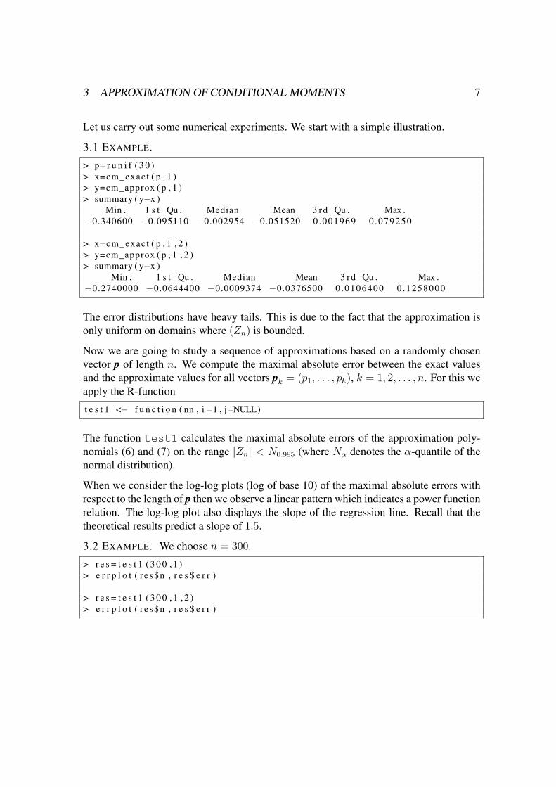
When we consider the log-log plots (log of base 10) of the maximal absolute errors withrespect to the length of p then we observe a linear pattern which indicates a power functionrelation. The log-log plot also displays the slope of the regression line. Recall that thetheoretical results predict a slope of 1.5.
3.2 EXAMPLE. We choose n = 300.
> r e s = t e s t 1 ( 3 0 0 , 1 )> e r r p l o t ( r e s$n , r e s $ e r r )
> r e s = t e s t 1 ( 3 0 0 , 1 , 2 )> e r r p l o t ( r e s$n , r e s $ e r r )
3 APPROXIMATION OF CONDITIONAL MOMENTS 8
●
●●
●●●
●●
●●●●●●
●●●●
●●●●●
●●●●●●
●
●●●●●●●●●
●
●●●
●●●●●●●
●●●●●●●●●●●●●●●●
●●●●●●●●●●●●●●●●●●●●●●●●●●●●●●●●●●●●●●●●●●●●●●●●●●●●●●●●●●●●●●●●●●●●●●●●●●●
●●●●●●●●●●●●●●●●●●●●●●●●●●●●●●●●●●●●●●●●●●●●●●●●●●●●●●●●●●●●●●●●●●●●●●●●●●●●●●●●●●●●●●●●●●●●●●●●●●●●●●●●●●●●●●●●●●●●●●●●●●●●●●●●●●●●●●●●●●●●●●●●●●●●●●
1.0 1.5 2.0 2.5
−3.
5−
2.5
−1.
5
n
err
slope = −1.6
●●
●●●●
●●
●
●●●●●
●●
●●●●●
●●●
●●●
●●●●●●
●
●●●●●●●●●●●●●●
●●●●●●●●●●
●●●●●●●●●●
●●●●●●●●●●●●●●●
●●●●●●●●●●●●●●●●●●●●●●
●●●●●●●●●●●●●●●●●●●●●●●●●●●●●●●●●●●●●●●●●●●●●●●●●●●●●●●●●●●●●●●●●●●●●●●●●●●●●●●●●●●●●●●●●●●●●●●●●●●●●●●●●●●●●●●●●●●●●●●●●●●●●●●●●●●●●●●●●●●●●●●●●●●●●●●●●●●●●●●●●●●●●●●●●●●●●●●●●●●●●●●●●●
1.0 1.5 2.0 2.5
−3.
5−
3.0
−2.
5−
2.0
−1.
5
ner
r
slope = −1.486
These numerical results support the quality of the theoretical error bounds.
The next step is the approximation of the conditional covariance matrix Fns based on thepreceding approximations of the conditional moments. This coded by the R-function (seesection 7)
vcond_approx <− f u n c t i o n ( p )
This function simply collects the results of cm_approx and puts them into an array. Thequality of approximation is the same as for the single components.
Things are becoming much more interesting when we pass to the expectation Fn of theconditional covariance matrix Fns. Theorem 2.4 in Strasser [1] shows that Fn can beapproximated with very simple expressions. These expressions are far simpler than thosewhich we would obtain by proceeding in a similar way as in (5). The approximations areof a considerably higher order and are valid in a stronger sense.
The matrix norm of a positive semidefinite symmetric matrix is defined by
||A|| = sup{x′Ax : ||x|| = 1}, (8)
(see the R-function nm in 7.) Let
Gn,ij := viδij −vivjσ2n
(9)
andHn,ij := Gn,ij +
vivjτiτj2σ4
n
(10)
Then it is shown in Theorem 2.4 of Strasser [1] and in Corollary 2.2 of Strasser [2] that
Fn = Gn +O(n−2) and ||Fn − Gn|| = O(n−1) (11)
3 APPROXIMATION OF CONDITIONAL MOMENTS 9
andFn = Hn +O(n−5/2) and ||Fn −Hn|| = O(n−3/2) (12)
The matrices Gn and Hn are coded by the R-functions (see section 7)
v_approx <− f u n c t i o n ( p , l i n e a r =FALSE)
The option linear returns Gn, otherwise Hn is returned. Let us consider some numericexamples.
3.3 EXAMPLE. We randomly choose 100 vectors p of length n = 20 and compare Fn
with Gn and Hn, respectively.
x= numer ic ( 0 )y=xz=xu=xf o r ( i i n 1 : 1 0 0 ) {
p= r u n i f ( 2 0 )a= v _ e x a c t ( p )b= v_approx ( p , l i n e a r =TRUE)c= v_approx ( p , l i n e a r =FALSE)x=c ( x , max ( abs ( a−b ) ) )y=c ( y , max ( abs ( a−c ) ) )z=c ( z , nm( a−b ) )u=c ( z , nm( a−c ) )}
> summary ( x )Min . 1 s t Qu . Median Mean 3 rd Qu . Max .
0 .0003435 0 .0004523 0 .0005354 0 .0005738 0 .0006347 0 .0015420> summary ( y )
Min . 1 s t Qu . Median Mean 3 rd Qu . Max .2 .133 e−05 3 .531 e−05 4 .502 e−05 5 .468 e−05 6 .122 e−05 2 .304 e−04> summary ( z )
Min . 1 s t Qu . Median Mean 3 rd Qu . Max .0 .001845 0 .003498 0 .004385 0 .004427 0 .005044 0 .008277> summary ( u )
Min . 1 s t Qu . Median Mean 3 rd Qu . Max .0 .0002906 0 .0034340 0 .0043570 0 .0043860 0 .0050170 0 .0082770
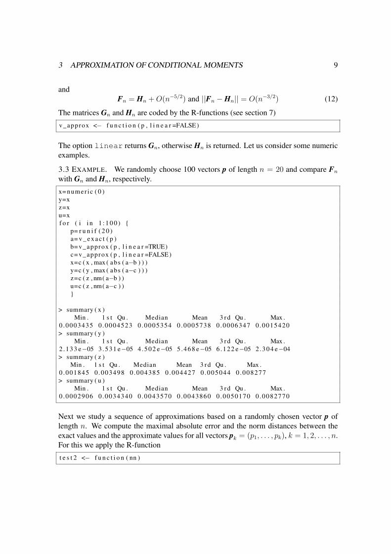
Next we study a sequence of approximations based on a randomly chosen vector p oflength n. We compute the maximal absolute error and the norm distances between theexact values and the approximate values for all vectors pk = (p1, . . . , pk), k = 1, 2, . . . , n.For this we apply the R-function
t e s t 2 <− f u n c t i o n ( nn )
3 APPROXIMATION OF CONDITIONAL MOMENTS 10
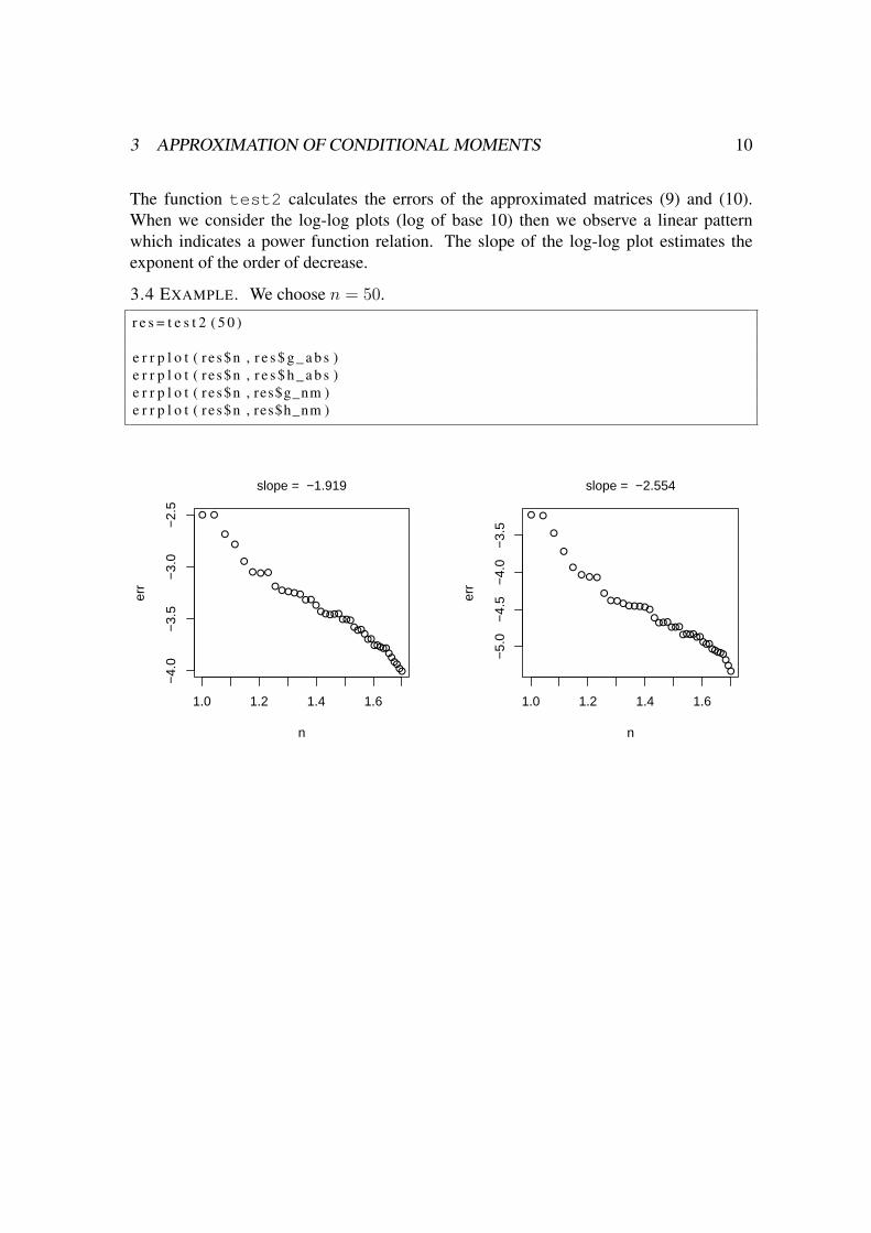
The function test2 calculates the errors of the approximated matrices (9) and (10).When we consider the log-log plots (log of base 10) then we observe a linear patternwhich indicates a power function relation. The slope of the log-log plot estimates theexponent of the order of decrease.
3.4 EXAMPLE. We choose n = 50.
r e s = t e s t 2 ( 5 0 )
e r r p l o t ( r e s$n , r e s $ g _ a b s )e r r p l o t ( r e s$n , r e s $ h _ a b s )e r r p l o t ( r e s$n , res$g_nm )e r r p l o t ( r e s$n , res$h_nm )
● ●
●
●
●
● ●●
●●●●●
●●●
●●●●●●●●
●●●●●●
●●●●●●●●●
●●
1.0 1.2 1.4 1.6
−4.
0−
3.5
−3.
0−
2.5
n
err
slope = −1.919
● ●
●
●
●● ●●
●●●●●●●●●
●●●●
●●●●●●●●●
●●●●●●●●
●●●
1.0 1.2 1.4 1.6
−5.
0−
4.5
−4.
0−
3.5
n
err
slope = −2.554
3 APPROXIMATION OF CONDITIONAL MOMENTS 11
● ●
● ●●
● ●●●●
●●●●●●●●
●●●
●●●
●●●●●●●●●
●●●●●●●●
1.0 1.2 1.4 1.6
−2.
6−
2.4
−2.
2−
2.0
n
err
slope = −0.784
● ●
● ●
●
● ●●
●●●●●●●●●
●●●●
●●●●●●●
●●●●●
●●●●●●●●
1.0 1.2 1.4 1.6
−4.
0−
3.5
−3.
0
ner
r
slope = −1.844
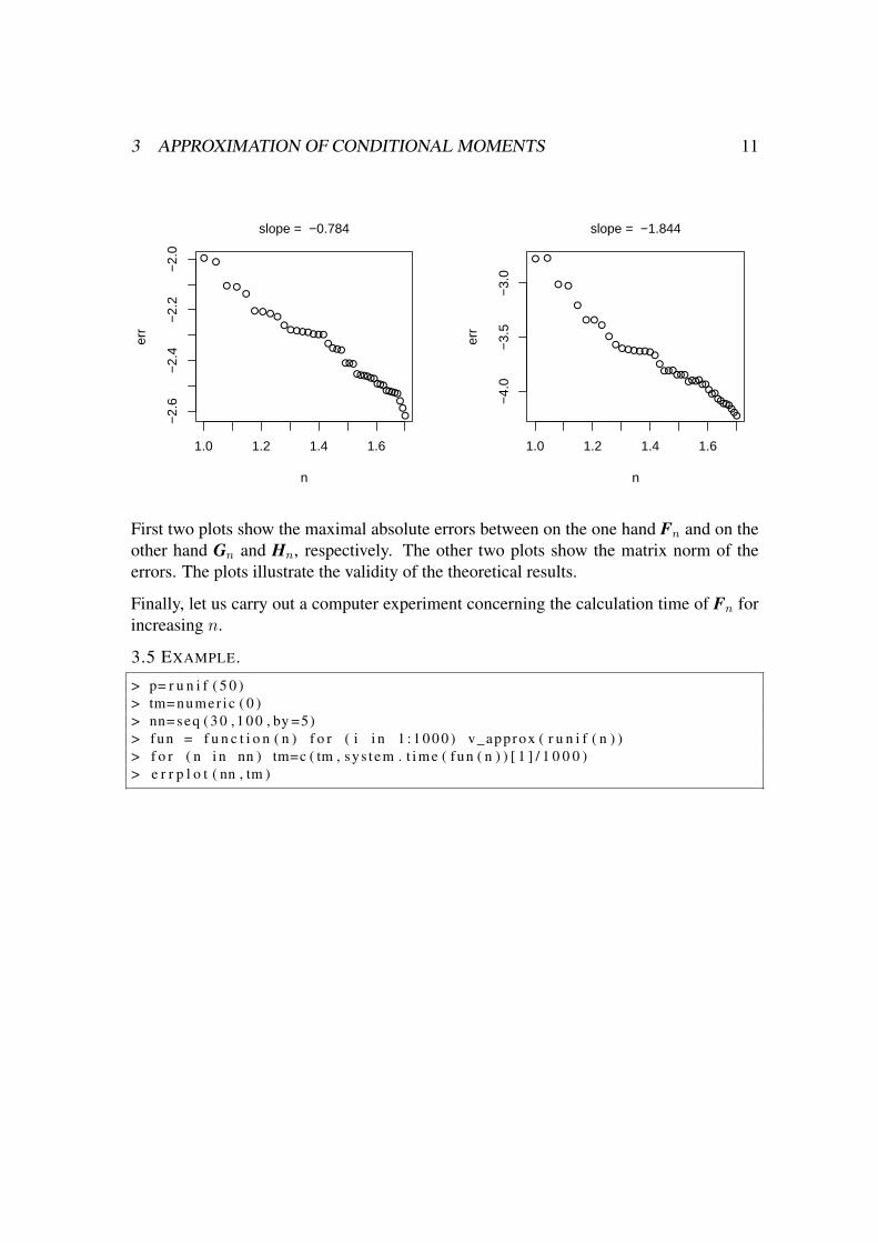
First two plots show the maximal absolute errors between on the one hand Fn and on theother hand Gn and Hn, respectively. The other two plots show the matrix norm of theerrors. The plots illustrate the validity of the theoretical results.
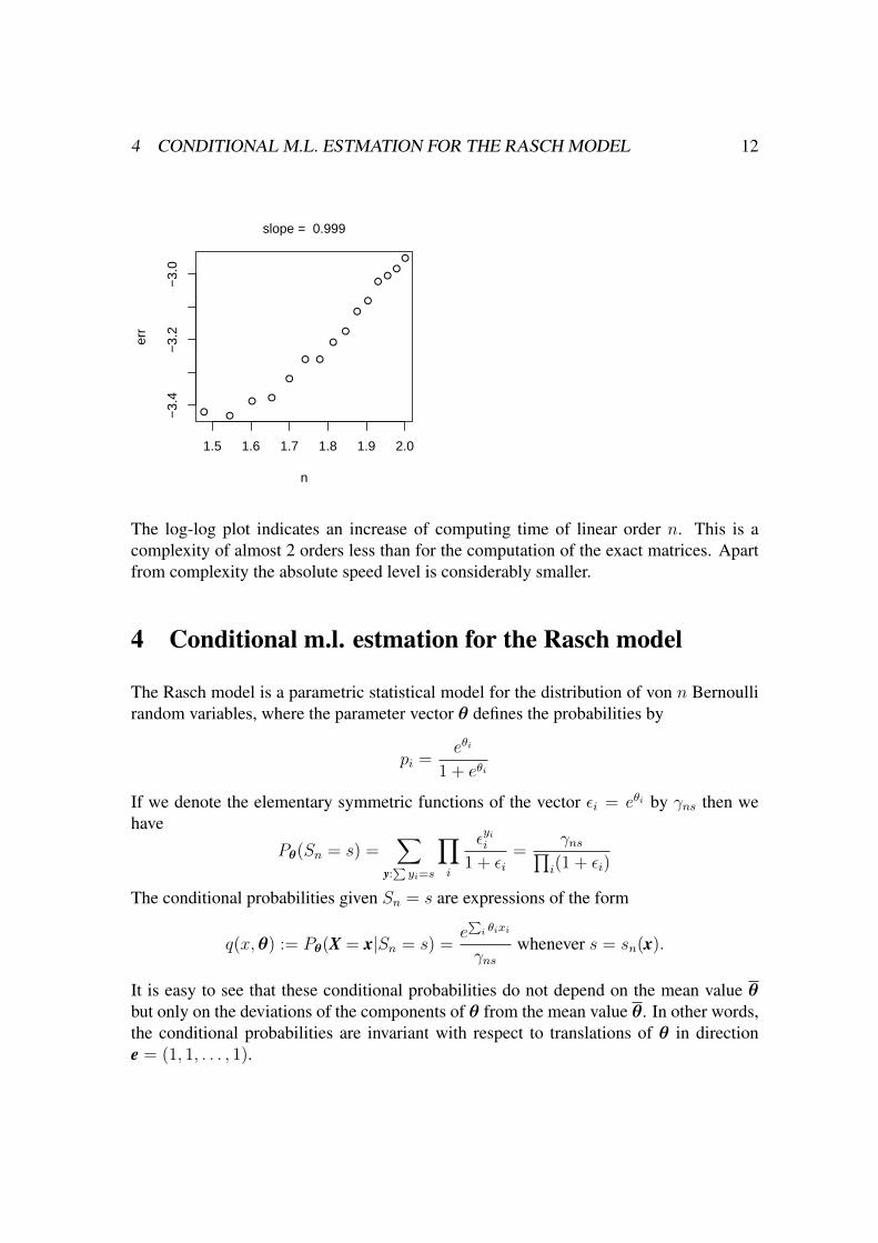
Finally, let us carry out a computer experiment concerning the calculation time of Fn forincreasing n.
3.5 EXAMPLE.
> p= r u n i f ( 5 0 )> tm= numer ic ( 0 )> nn= seq ( 3 0 , 1 0 0 , by =5)> fun = f u n c t i o n ( n ) f o r ( i i n 1 : 1 0 0 0 ) v_approx ( r u n i f ( n ) )> f o r ( n i n nn ) tm=c ( tm , sys tem . t ime ( fun ( n ) ) [ 1 ] / 1 0 0 0 )> e r r p l o t ( nn , tm )
4 CONDITIONAL M.L. ESTMATION FOR THE RASCH MODEL 12
● ●
● ●
●
● ●
●
●
●
●
●●
●
●
1.5 1.6 1.7 1.8 1.9 2.0
−3.
4−
3.2
−3.
0
n
err
slope = 0.999
The log-log plot indicates an increase of computing time of linear order n. This is acomplexity of almost 2 orders less than for the computation of the exact matrices. Apartfrom complexity the absolute speed level is considerably smaller.
4 Conditional m.l. estmation for the Rasch model
The Rasch model is a parametric statistical model for the distribution of von n Bernoullirandom variables, where the parameter vector θ defines the probabilities by
pi =eθi
1 + eθi
If we denote the elementary symmetric functions of the vector εi = eθi by γns then wehave
Pθ(Sn = s) =∑
y:∑yi=s
∏i
εyii1 + εi
=γns∏
i(1 + εi)
The conditional probabilities given Sn = s are expressions of the form
q(x,θ) := Pθ(X = x|Sn = s) =e∑
i θixi
γnswhenever s = sn(x).
It is easy to see that these conditional probabilities do not depend on the mean value θbut only on the deviations of the components of θ from the mean value θ. In other words,the conditional probabilities are invariant with respect to translations of θ in directione = (1, 1, . . . , 1).
4 CONDITIONAL M.L. ESTMATION FOR THE RASCH MODEL 13
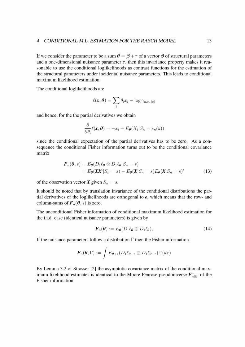
If we consider the parameter to be a sum θ = β+ τ of a vector β of structural parametersand a one-dimensional nuisance parameter τ , then this invariance property makes it rea-sonable to use the conditional loglikelihoods as contrast functions for the estimation ofthe structural parameters under incidental nuisance parameters. This leads to conditionalmaximum likelihood estimation.
The conditional loglikelihoods are
`(x,θ) =∑i
θixi − log γn,sn(x)
and hence, for the the partial derivatives we obtain
∂
∂θi`(x,θ) = −xi + Eθ(Xi|Sn = sn(x))
since the conditional expectation of the partial derivatives has to be zero. As a con-sequence the conditional Fisher information turns out to be the conditional covariancematrix
Fn(θ, s) = Eθ(D1`θ ⊗D1`θ|Sn = s)
= Eθ(XXt|Sn = s)− Eθ(X|Sn = s)Eθ(X|Sn = s)t (13)
of the observation vector X given Sn = s.
It should be noted that by translation invariance of the conditional distributions the par-tial derivatives of the loglikelihoods are orthogonal to e, which means that the row- andcolumn-sums of Fn(θ, s) is zero.
The unconditional Fisher information of conditional maximum likelihood estimation forthe i.i.d. case (identical nuisance parameters) is given by
Fn(θ) := Eθ(D1`θ ⊗D1`θ), (14)
If the nuisance parameters follow a distribution Γ then the Fisher information
Fn(θ,Γ) :=
∫Eθ+τ (D1`θ+τ ⊗D1`θ+τ ) Γ(dτ)
By Lemma 3.2 of Strasser [2] the asymptotic covariance matrix of the conditional max-imum likelihood estimates is identical to the Moore-Penrose pseudoinverse F+
nβΓ of theFisher information.
5 EXACT CALCULATIONS FOR THE RASCH MODEL 14
5 Exact calculations for the Rasch model
Let θ = β + τ where β = 0.
It is clear form the preceding section 4 that the Fisher information in the i.i.d. case can becalculated as the expectation of the conditional covariance matrix
Fnβτ := Fn(θ) = Eθ
(Eθ(XXt|Sn = s)− Eθ(X|Sn = s)Eθ(X|Sn = s)t
).
In the case of a random nuisance parameter with distribution Γ we have
FnβΓ := Fn(θ,Γ) =
∫Fnτ Γ(dτ)
The exact calculation of FnβΓ for an empirical distribution Γ is coded by the R-function
f _ e x a c t <− f u n c t i o n ( be t a , t a u =0)
The parameter tau contains the data vector for the empirical distribution Γ.
The exact calculation of the asymptotic covariance matrix F+nβΓ can be obtained as the
Moore-Penrose pseudoinverse which is coded by the R-function
p inv <− f u n c t i o n ( x , eps =1e−10)
6 Approximations for the Rasch model
6.1 The Fisher information
The most simple approximation of the Fisher information for the i.i.d. case is given byequation (9) which now is a function of β and τ . In the case of a random nuisanceparameter the approximation provide by equation (9) is
GnβΓ :=
∫Gnβτ Γ(dτ)
A more sophisticated approximation is provided by equation (10) leading to
HnβΓ :=
∫Hnβτ Γ(dτ)
This approximations are coded by the R-function
6 APPROXIMATIONS FOR THE RASCH MODEL 15
f _ a p p r o x <− f u n c t i o n ( be t a , t a u =0 , l i n e a r =FALSE)
Let us consider some numeric examples.
6.1 EXAMPLE. We randomly choose 100 vectors β of length n = 20 and a vector oflength 20 of nuisance parameters τ . We compare FnβΓ with GnβΓ) and HnβΓ) where Γ isthe empirical distribution the nuisance parameter.
> x= numer ic ( 0 )> y=x> z=x> u=x> f o r ( i i n 1 : 1 0 0 ) {+ b e t a =rnorm ( 2 0 )+ t a u =rnorm ( 2 0 )+ a= f _ e x a c t ( be t a , t a u )+ b= f _ a p p r o x ( be t a , t au , l i n e a r =TRUE)+ c= f _ a p p r o x ( be t a , t au , l i n e a r =FALSE)+ x=c ( x , max ( abs ( a−b ) ) )+ y=c ( y , max ( abs ( a−c ) ) )+ z=c ( z , nm( a−b ) )+ u=c ( z , nm( a−c ) )+ }> summary ( x )
Min . 1 s t Qu . Median Mean 3 rd Qu . Max .0 .0001906 0 .0003882 0 .0004514 0 .0004858 0 .0005404 0 .0008830> summary ( y )
Min . 1 s t Qu . Median Mean 3 rd Qu . Max .1 .050 e−05 3 .549 e−05 5 .092 e−05 6 .724 e−05 8 .364 e−05 2 .819 e−04> summary ( z )
Min . 1 s t Qu . Median Mean 3 rd Qu . Max .0 .001226 0 .001956 0 .002280 0 .002323 0 .002688 0 .003832> summary ( u )
Min . 1 s t Qu . Median Mean 3 rd Qu . Max .9 .708 e−05 1 .937 e−03 2 .254 e−03 2 .301 e−03 2 .685 e−03 3 .832 e−03
Next we study a sequence of approximations based on a randomly chosen vector β oflength n. We compute the errors between the exact values and the approximate values forall vectors βk = (β1, . . . , βk), k = 1, 2, . . . , n. For this we apply the R-function
t e s t 3 <− f u n c t i o n ( nn )
The function test3 calculates the errors of the approximated matrices (9) and (10).When we consider the log-log plots (log of base 10) then we observe a linear patternwhich indicates a power function relation. The slope of the log-log plot estimates the
6 APPROXIMATIONS FOR THE RASCH MODEL 16
exponent of the order of decrease.
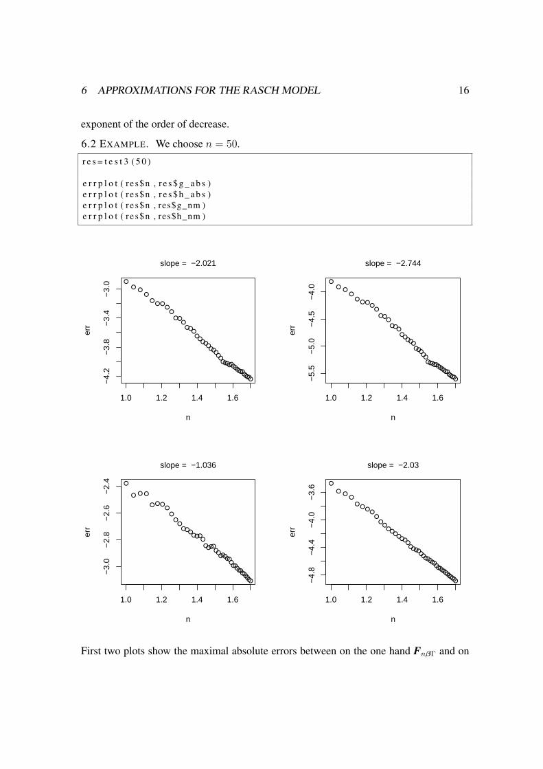
6.2 EXAMPLE. We choose n = 50.
r e s = t e s t 3 ( 5 0 )
e r r p l o t ( r e s$n , r e s $ g _ a b s )e r r p l o t ( r e s$n , r e s $ h _ a b s )e r r p l o t ( r e s$n , res$g_nm )e r r p l o t ( r e s$n , res$h_nm )
●●
●●
●● ●
●●
●●●
●●●
●●
●●●●●●
●●●●●●●●●●●●●●●●●●
1.0 1.2 1.4 1.6
−4.
2−
3.8
−3.
4−
3.0
n
err
slope = −2.021
●●
●●
●● ●
●●
●●●
●●●●
●●●●
●●●●●
●●●●●●●●●●●●●●●●
1.0 1.2 1.4 1.6
−5.
5−
5.0
−4.
5−
4.0
n
err
slope = −2.744
●
● ● ●
● ● ●●
●●
●●●●
●●●●
●●●●●●
●●●●●●●●●●●●●●●●●
1.0 1.2 1.4 1.6
−3.
0−
2.8
−2.
6−
2.4
n
err
slope = −1.036
●
●●
●
●●
●●
●●
●●●
●●●●
●●●●●
●●●●●●●●●●●●●●●●●●●
1.0 1.2 1.4 1.6
−4.
8−
4.4
−4.
0−
3.6
n
err
slope = −2.03
First two plots show the maximal absolute errors between on the one hand FnβΓ and on
6 APPROXIMATIONS FOR THE RASCH MODEL 17
the other hand GnβΓ and HnβΓ, respectively. The other two plots show the matrix normof the errors. The plots illustrate the validity of the theoretical results.
6.2 The asymptotic covariance matrix
Basically the asymptotic covariance matrix can be approximated by calculating dieMoore-Penrose pseudoinverse of the approximate Fisher information. This is proved byStrasser [2] in Theorems 2.3 and 2.4. Moore-Penrose pseudoinverses can be calculatedby well-known algorithms (see the R-function pinv in section 7).
Let us perform the same numerical experiments as for the Fisher information.
6.3 EXAMPLE. We randomly choose 100 vectors β of length n = 30 and a vector oflength 30 of nuisance parameters τ . We compare F+
nβΓ with G+nβΓ and H+
nβΓ where Γ isthe empirical distribution the nuisance parameter.
> x= numer ic ( 0 )> y=x> z=x> u=x> f o r ( i i n 1 : 1 0 0 ) {+ b e t a =rnorm ( 3 0 )+ t a u =rnorm ( 3 0 )+ a= p inv ( f _ e x a c t ( be t a , t a u ) )+ b= p inv ( f _ a p p r o x ( be t a , t au , l i n e a r =TRUE ) )+ c= p inv ( f _ a p p r o x ( be t a , t au , l i n e a r =FALSE ) )+ x=c ( x , max ( abs ( a−b ) ) )+ y=c ( y , max ( abs ( a−c ) ) )+ z=c ( z , nm( a−b ) )+ u=c ( z , nm( a−c ) )+ }> summary ( x )
Min . 1 s t Qu . Median Mean 3 rd Qu . Max .0 .004479 0 .015140 0 .021880 0 .030950 0 .032700 0 .189100> summary ( y )
Min . 1 s t Qu . Median Mean 3 rd Qu . Max .0 .0001929 0 .0010270 0 .0020750 0 .0045350 0 .0040890 0 .0519000> summary ( z )
Min . 1 s t Qu . Median Mean 3 rd Qu . Max .0 .03998 0 .06354 0 .08139 0 .08703 0 .10280 0 .23680> summary ( u )
Min . 1 s t Qu . Median Mean 3 rd Qu . Max .0 .001983 0 .062670 0 .080620 0 .086190 0 .102600 0 .236800
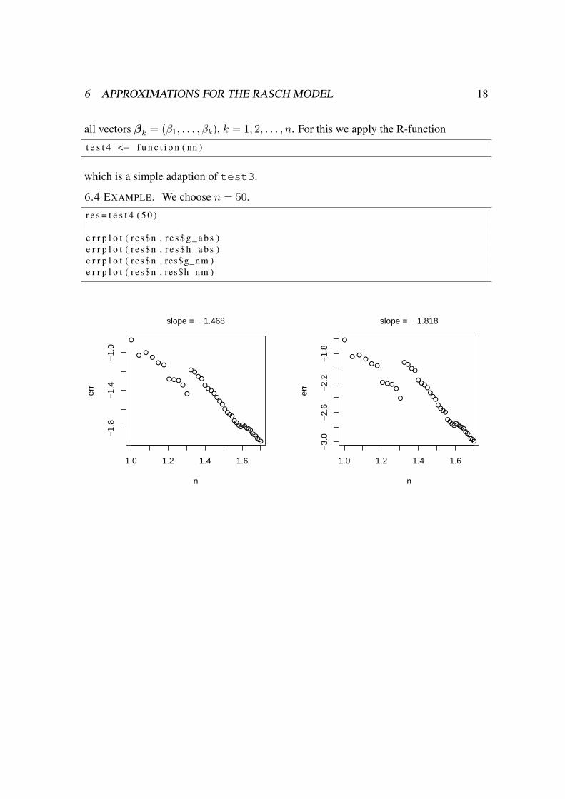
Next we study a sequence of approximations based on a randomly chosen vector β oflength n. We compute the errors between the exact values and the approximate values for
6 APPROXIMATIONS FOR THE RASCH MODEL 18
all vectors βk = (β1, . . . , βk), k = 1, 2, . . . , n. For this we apply the R-function
t e s t 4 <− f u n c t i o n ( nn )
which is a simple adaption of test3.
6.4 EXAMPLE. We choose n = 50.
r e s = t e s t 4 ( 5 0 )
e r r p l o t ( r e s$n , r e s $ g _ a b s )e r r p l o t ( r e s$n , r e s $ h _ a b s )e r r p l o t ( r e s$n , res$g_nm )e r r p l o t ( r e s$n , res$h_nm )
●
●●
●● ●
●●●●
●
●●●●
●●●
●●●●●●●●
●●●●●●●●●●●●●●●
1.0 1.2 1.4 1.6
−1.
8−
1.4
−1.
0
n
err
slope = −1.468
●
● ●●
● ●
●●●●
●
●●●●
●●●
●●●●●●●●
●●●●●●●●●●●●
●●●
1.0 1.2 1.4 1.6
−3.
0−
2.6
−2.
2−
1.8
n
err
slope = −1.818
7 APPENDIX: R-CODE 19
●
● ●
●
●●
●●●
●●
●●
●●●
●●
●●●●●●●●
●●●●●●●●●●●●●●●
1.0 1.2 1.4 1.6
−1.
4−
1.2
−1.
0−
0.8
−0.
6
n
err
slope = −1.14
●
● ●●
● ●
●●●●
●
●●●●
●●●
●●●●●●●●
●●●●●●●●●●●●
●●●
1.0 1.2 1.4 1.6
−2.
8−
2.4
−2.
0−
1.6
ner
r
slope = −1.783
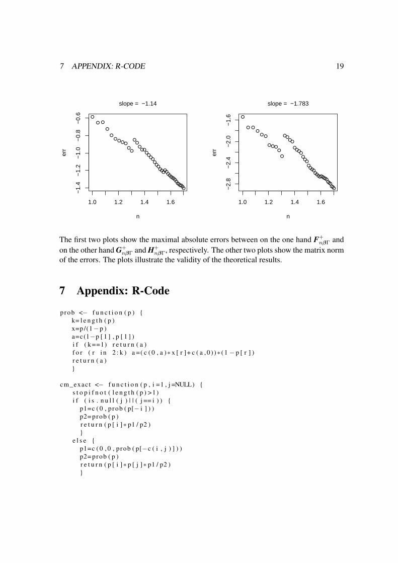
The first two plots show the maximal absolute errors between on the one hand F+nβΓ and
on the other hand G+nβΓ and H+
nβΓ, respectively. The other two plots show the matrix normof the errors. The plots illustrate the validity of the theoretical results.
7 Appendix: R-Code
prob <− f u n c t i o n ( p ) {k= l e n g t h ( p )x=p /(1−p )a=c(1−p [ 1 ] , p [ 1 ] )i f ( k ==1) r e t u r n ( a )f o r ( r i n 2 : k ) a =( c ( 0 , a )∗ x [ r ]+ c ( a , 0 ) )∗ ( 1 − p [ r ] )r e t u r n ( a )}
cm_exact <− f u n c t i o n ( p , i =1 , j =NULL) {s t o p i f n o t ( l e n g t h ( p ) >1)i f ( i s . n u l l ( j ) | | ( j == i ) ) {
p1=c ( 0 , prob ( p[− i ] ) )p2= prob ( p )r e t u r n ( p [ i ]∗ p1 / p2 )}
e l s e {p1=c ( 0 , 0 , p rob ( p[−c ( i , j ) ] ) )p2= prob ( p )r e t u r n ( p [ i ]∗ p [ j ]∗ p1 / p2 )}
7 APPENDIX: R-CODE 20
}
v c o n d _ e x a c t <− f u n c t i o n ( p ) {k= l e n g t h ( p )m= m a t r i x ( 0 , k , k +1)f = a r r a y ( 0 , c ( k , k , k + 1 ) )f o r ( i i n 1 : k ) {
m[ i , ] = cm_exact ( p , i )f [ i , i , ] =m[ i ,]−m[ i , ] ^ 2}
f o r ( i i n 1 : ( k−1)) f o r ( j i n ( i + 1 ) : k ) {f [ i , j , ] = cm_exact ( p , i , j )−m[ i , ] ∗m[ j , ]f [ j , i , ] = f [ i , j , ]}
r e t u r n ( f )}
v _ e x a c t <− f u n c t i o n ( p ) {k= l e n g t h ( p )q= prob ( p )c f = v c o n d _ e x a c t ( p )f = m a t r i x ( 0 , k , k )f o r ( s i n 1 : ( k + 1 ) ) f = f + c f [ , , s ]∗ q [ s ]r e t u r n ( f )}
cm_approx <− f u n c t i o n ( p , i =1 , j =NULL) {s t o p i f n o t ( l e n g t h ( p ) >1)n= l e n g t h ( p )v=p∗(1−p )s s =sum ( v )z = ( 0 : n−sum ( p ) ) / s q r t ( s s )t a u =2∗ ( p−sum ( v∗p ) / s s )i f ( i s . n u l l ( j ) | | ( j == i ) )
r e t u r n ( p [ i ]+ v [ i ]∗ z / s q r t ( s s )−v [ i ]∗ t a u [ i ] ∗ ( z ^2−1) / (2∗ s s ) )e l s e {
a=p [ i ]∗ p [ j ]b=p [ i ]∗ v [ j ]+ p [ j ]∗ v [ i ]c=v [ i ]∗ v [ j ]d=p [ i ]∗ v [ j ]∗ t a u [ j ]+ p [ j ]∗ v [ i ]∗ t a u [ i ]r e t u r n ( a+b∗z / s q r t ( s s ) + ( z ^2−1)∗( c−d / 2 ) / s s )}
}
rng <− f u n c t i o n ( p , l v = 0 . 9 9 ) {n= l e n g t h ( p )s =0: nv=p∗(1−p )
7 APPENDIX: R-CODE 21
z =( s−sum ( p ) ) / s q r t ( sum ( v ) )i =which ( abs ( z ) < qnorm ( l v +(1− l v ) / 2 ) )r e t u r n ( i )}
vcond_approx <− f u n c t i o n ( p ) {k= l e n g t h ( p )m= m a t r i x ( 0 , k , k +1)f = a r r a y ( 0 , c ( k , k , k + 1 ) )f o r ( i i n 1 : k ) {
m[ i , ] = cm_approx ( p , i )f [ i , i , ] =m[ i ,]−m[ i , ] ^ 2}
f o r ( i i n 1 : ( k−1)) f o r ( j i n ( i + 1 ) : k ) {f [ i , j , ] = cm_approx ( p , i , j )−m[ i , ] ∗m[ j , ]f [ j , i , ] = f [ i , j , ]}
r e t u r n ( f )}
t e s t 1 <− f u n c t i o n ( nn , i =1 , j =NULL) {i f ( i s . n u l l ( j ) ) j = ie= numer ic ( 0 )p0= r u n i f ( nn )m=max ( c ( i , j , 1 0 ) )nn=max (m, nn )f o r ( n i n m: nn ) {
p=p0 [ 1 : n ]s= rng ( p )x= cm_exact ( p , i , j ) [ s ]y=cm_approx ( p , i , j ) [ s ]e=c ( e , max ( abs ( x−y ) ) )}
r e t u r n ( l i s t ( n=m: nn , e r r =e ) )}
e r r p l o t <− f u n c t i o n ( n , e ) {windows ( 4 , 4 )p l o t ( log10 ( n ) , log10 ( e ) , x l a b =" n " , y l a b =" e r r " )fm=lm ( log10 ( e )~ log10 ( n ) )mtex t ( p a s t e ( " s l o p e =" , round ( fm$coef [ 2 ] , 3 ) ) , 3 , 1 )}
v_approx <− f u n c t i o n ( p , l i n e a r =FALSE) {v=p∗(1−p )i f ( l i n e a r ) r e t u r n ( d i a g ( v)− o u t e r ( v , v ) / sum ( v ) )e l s e {
c3=p∗(1−p )∗(1−2∗p )w=(2∗p−1)/ s q r t ( mean ( v ) ) + mean ( c3 ) / mean ( v ) ^ ( 3 / 2 )
7 APPENDIX: R-CODE 22
r e t u r n ( d i a g ( v)− o u t e r ( v , v ) / sum ( v )∗ ( 1 + o u t e r (w,w ) / 2 / l e n g t h ( p ) ) )}
}
nm <− f u n c t i o n ( a ) s q r t ( max ( e i g e n ( t ( a)%∗%a ) $ v a l u e s ) )
t e s t 2 <− f u n c t i o n ( nn ) {p0= r u n i f ( nn )m=10nn=max (m, nn )x= numer ic ( 0 )y=xz=xu=xf o r ( n i n m: nn ) {
Cat ( n )p=p0 [ 1 : n ]a= v _ e x a c t ( p )b= v_approx ( p , l i n e a r =TRUE)c= v_approx ( p , l i n e a r =FALSE)x=c ( x , max ( abs ( a−b ) ) )y=c ( y , max ( abs ( a−c ) ) )z=c ( z , nm( a−b ) )u=c ( u , nm( a−c ) )}
r e t u r n ( l i s t ( n=m: nn , g_abs =x , h_abs =y , g_nm=z , h_nm=u ) )}
f _ e x a c t <− f u n c t i o n ( be t a , t a u =0) {b e t a = be t a−mean ( b e t a )k= l e n g t h ( b e t a )q= numer ic ( k +1)f o r ( i i n 1 : l e n g t h ( t a u ) )
q=q+ prob ( exp ( b e t a + t a u [ i ] ) / ( 1 + exp ( b e t a + t a u [ i ] ) ) )q=q / l e n g t h ( t a u )c f = v c o n d _ e x a c t ( exp ( b e t a ) / ( 1 + exp ( b e t a ) ) )f = m a t r i x ( 0 , k , k )f o r ( s i n 1 : ( k + 1 ) ) f = f + c f [ , , s ]∗ q [ s ]r e t u r n ( f )}
p inv <− f u n c t i o n ( x , eps =1e−10){y=svd ( x )dm=min ( dim ( x ) )chk=y$d > epsd = ( 1 / ( y$d+1−chk ) ) ∗ chkr e t u r n ( y$v%∗%d i a g ( d , dm , dm)%∗% t ( y$u ) )
7 APPENDIX: R-CODE 23
}
f _ a p p r o x <− f u n c t i o n ( be t a , t a u =0 , l i n e a r =FALSE) {b e t a = be t a−mean ( b e t a )k= l e n g t h ( b e t a )f = m a t r i x ( 0 , k , k )f o r ( i i n 1 : l e n g t h ( t a u ) ) {
p=exp ( b e t a + t a u [ i ] ) / ( 1 + exp ( b e t a + t a u [ i ] ) )f = f + v_approx ( p , l i n e a r = l i n e a r )
f = f / l e n g t h ( t a u )r e t u r n ( f )}
t e s t 3 <− f u n c t i o n ( nn ) {b e t a 0 =rnorm ( nn )t a u 0 =rnorm ( nn )m=10nn=max (m, nn )x= numer ic ( 0 )y=xz=xu=xf o r ( n i n m: nn ) {
Cat ( n )b e t a = b e t a 0 [ 1 : n ]t a u = t a u 0 [ 1 : n ]a= f _ e x a c t ( be t a , t a u )b= f _ a p p r o x ( be t a , t au , l i n e a r =TRUE)c= f _ a p p r o x ( be t a , t au , l i n e a r =FALSE)x=c ( x , max ( abs ( a−b ) ) )y=c ( y , max ( abs ( a−c ) ) )z=c ( z , nm( a−b ) )u=c ( u , nm( a−c ) )}
r e t u r n ( l i s t ( n=m: nn , g_abs =x , h_abs =y , g_nm=z , h_nm=u ) )}
t e s t 4 <− f u n c t i o n ( nn ) {b e t a 0 =rnorm ( nn )t a u 0 =rnorm ( nn )m=10nn=max (m, nn )x= numer ic ( 0 )y=xz=xu=xf o r ( n i n m: nn ) {
Cat ( n )b e t a = b e t a 0 [ 1 : n ]
REFERENCES 24
t a u = t a u 0 [ 1 : n ]a= p inv ( f _ e x a c t ( be t a , t a u ) )b= p inv ( f _ a p p r o x ( be t a , t au , l i n e a r =TRUE ) )c= p inv ( f _ a p p r o x ( be t a , t au , l i n e a r =FALSE ) )x=c ( x , max ( abs ( a−b ) ) )y=c ( y , max ( abs ( a−c ) ) )z=c ( z , nm( a−b ) )u=c ( u , nm( a−c ) )}
r e t u r n ( l i s t ( n=m: nn , g_abs =x , h_abs =y , g_nm=z , h_nm=u ) )}
References
[1] H. Strasser. Asymptotic expansions for conditional moments of Bernoulli trials. Tech-nical report, Institute of Statistics and Mathematics, WU, 2011.
[2] H. Strasser. The covariance structure of conditional maximum likelihood estimateswhen the number of item parameters is large. Technical report, Institute of Statisticsand Mathematics, WU, 2011.