Numerical Simulation of Colloidal Interaction

Dr P. E. Dyshlovenko

Ulyanovsk State Technical University, Russia

E-mail: pavel@ulstu.ru

WWW: http://people.ulstu.ru/~pavel/

2

Numerical Simulation of Colloidal Interaction

• Introduction• Numerical Method• Results• Conclusion

3

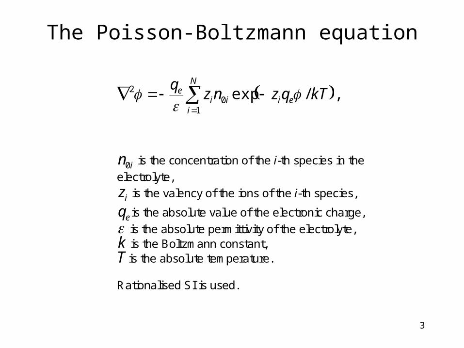
The Poisson-Boltzmann equation

N

ieiii

e kTqznzq

10

2 /exp

,

in0 is the concentration of the i-th species in the

electrolyte,

iz is the valency of the ions of the i-th species,

eq is the absolute value of the electronic charge,

is the absolute permittivity of the electrolyte, k is the Boltzmann constant, T is the absolute temperature. Rationalised SI is used.

4

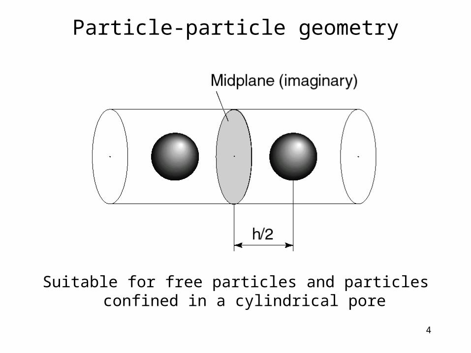
Particle-particle geometry

Suitable for free particles and particles confined in a cylindrical pore

5

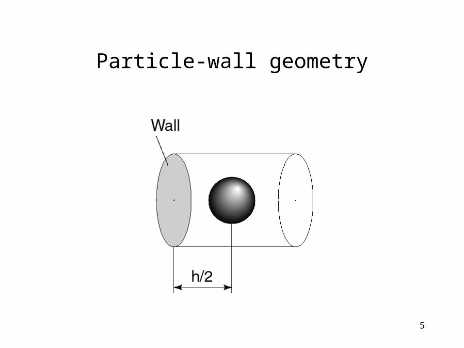
Particle-wall geometry

6

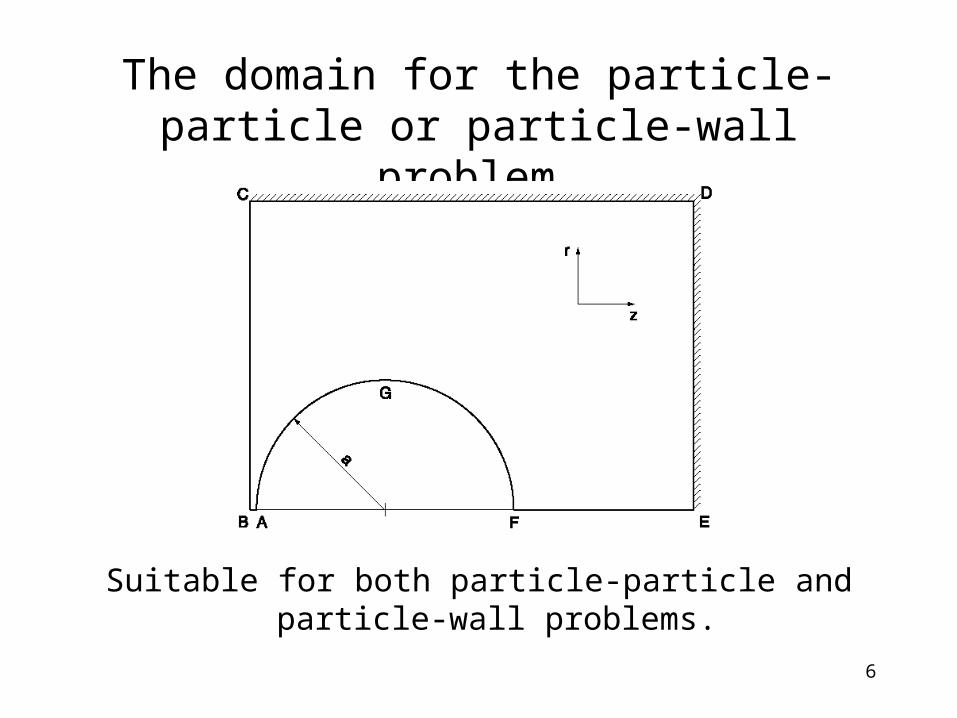
The domain for the particle-particle or particle-wall problem.

Suitable for both particle-particle and particle-wall problems.

7

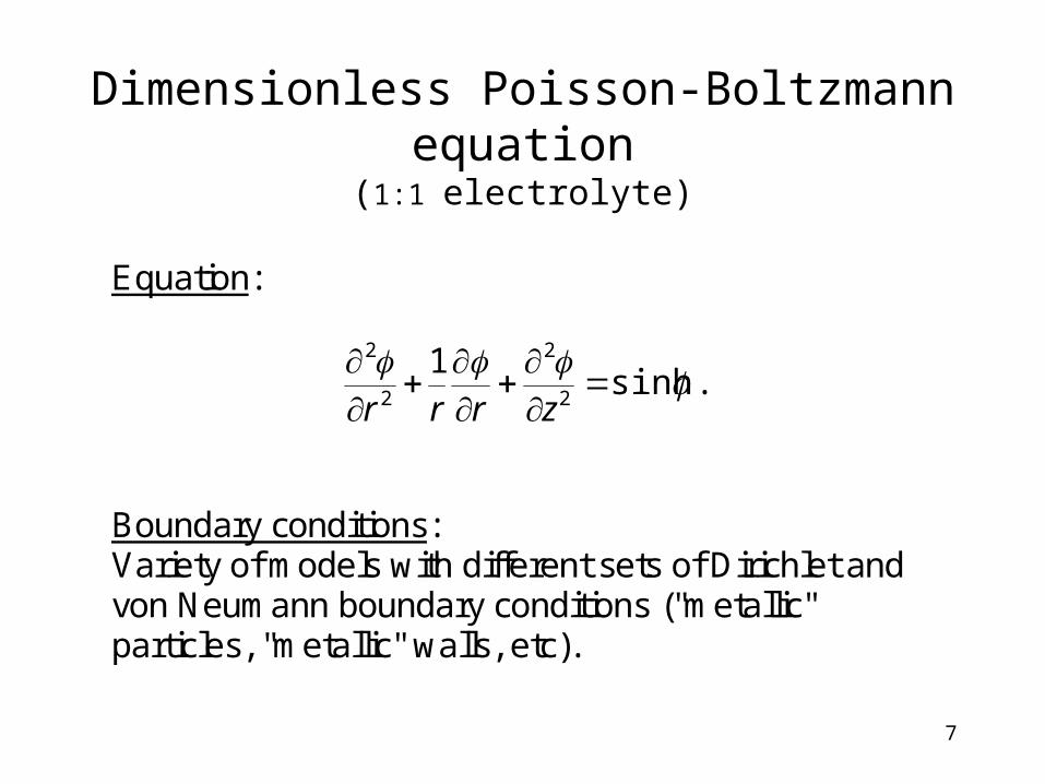
Dimensionless Poisson-Boltzmann equation

(1:1 electrolyte)

Equation:

sinh

12

2

2

2

zrrr.

Boundary conditions: Variety of models with different sets of Dirichlet and von Neumann boundary conditions ("metallic" particles, "metallic" walls, etc).

8

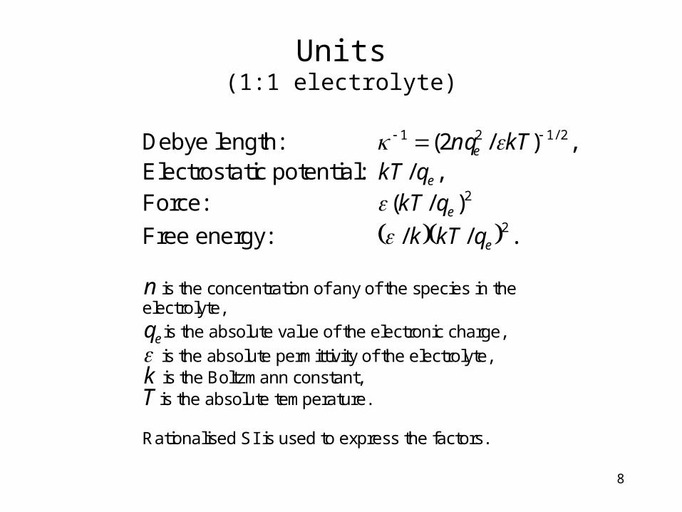
Units(1:1 electrolyte)

Debye length: 2/121 )/2( kTnqe , Electrostatic potential: eqkT / , Force: 2)/( eqkT

Free energy: 2// eqkTk . n is the concentration of any of the species in the electrolyte,

eq is the absolute value of the electronic charge,

is the absolute permittivity of the electrolyte, k is the Boltzmann constant, T is the absolute temperature. Rationalised SI is used to express the factors.

9

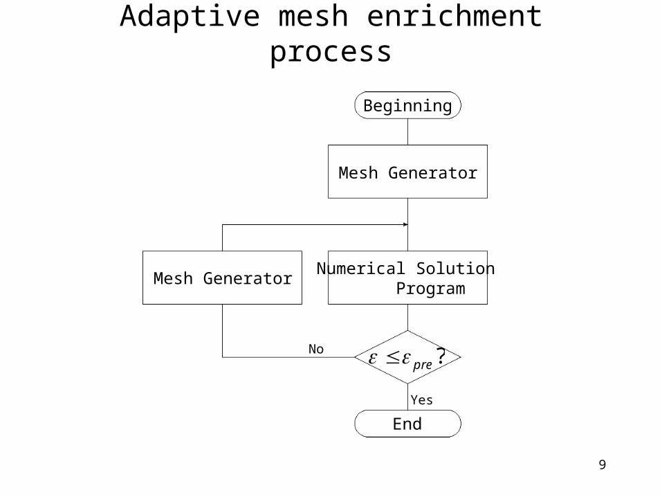
Adaptive mesh enrichment process

Beginning

End

Mesh Generator

Mesh GeneratorNumerical Solution Program

No

Yes

?pre

10

Numerical method

• Galerkin finite-element method• Irregular 2D mesh • Triangular elements• Quadratic approximation (six nodes on an

element)• Quasi-Newton method for the system of non-

linear algebraic equations• The sparse matrix technique

11

Mesh generator

• The mesh is a Delaunay Triangulation• Irregular mesh• Triangular elements• Any number of straight-line or round

boundaries.• Freely available at http://people.ulstu.ru/~pavel/

12

Error evaluation (1)

A posteriori error estimator O. C. Zienkiewicz and J. Z. Zhu, Int. J. Numer. Meth. Eng. 33, 1331 (1992). E - "finite-element" electric field, a gradient

of the FE potential. E

- "exact'' electric field, obtained by some kind of the gradient recovery technique. The error is defined as a deviation of one quantity from the other.

13

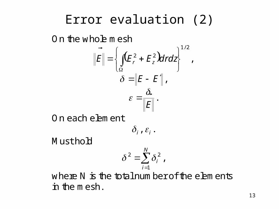
Error evaluation (2)

On the whole mesh

2/1

22

drdzEEE zr

,

EE

,

E .

On each element

i , i . Must hold

N

ii

1

22 ,

where N is the total number of the elements in the mesh.

14

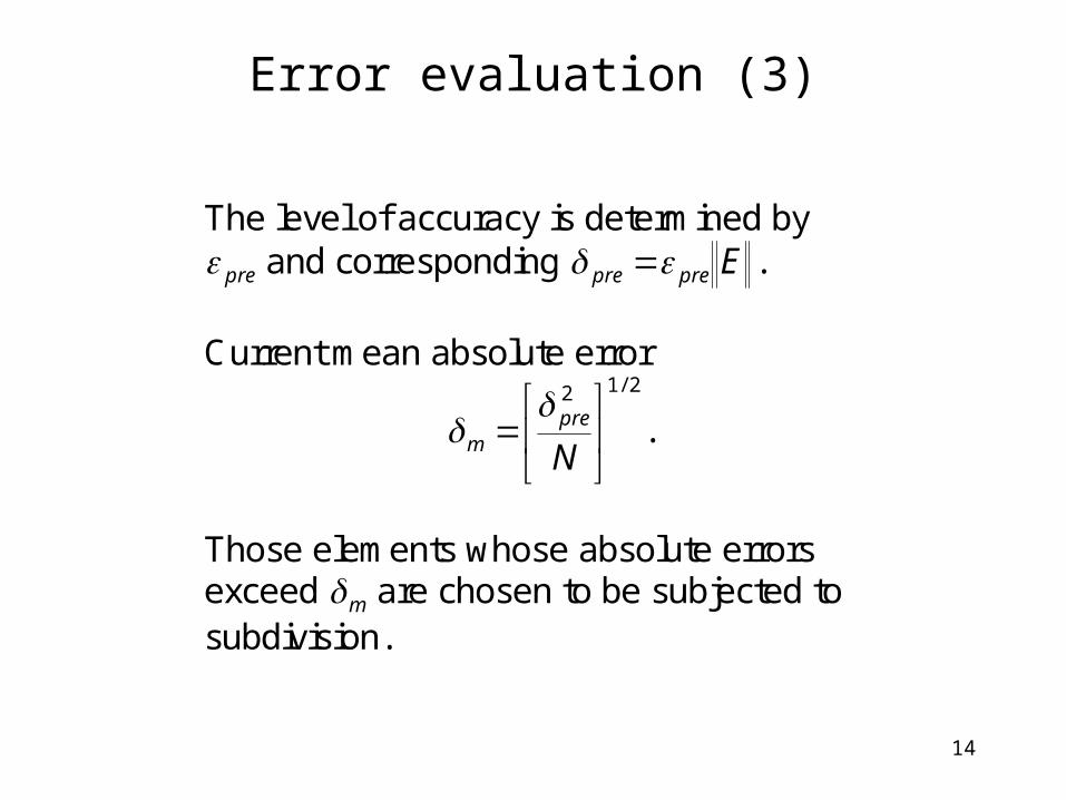
Error evaluation (3)

The level of accuracy is determined by

pre and corresponding Eprepre

.

Current mean absolute error

2/12

Npre

m

.

Those elements whose absolute errors exceed m are chosen to be subjected to subdivision.

15

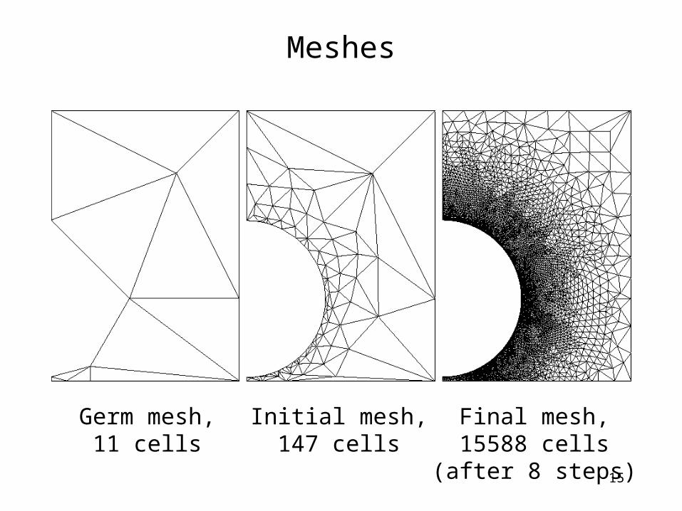
Meshes

Germ mesh,11 cells

Initial mesh,147 cells

Final mesh,15588 cells

(after 8 steps)

16

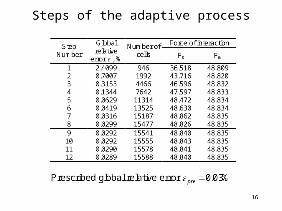
Steps of the adaptive process

Prescribed global relative error %03.0pre

Force of interaction Step Number

Global relative

error , %

Number of cells Fs Fm

1 2.4099 946 36.518 48.809 2 0.7007 1992 43.716 48.820 3 0.3153 4466 46.596 48.832 4 0.1344 7642 47.597 48.833 5 0.0629 11314 48.472 48.834 6 0.0419 13525 48.630 48.834 7 0.0316 15187 48.862 48.835 8 0.0299 15477 48.826 48.835 9 0.0292 15541 48.840 48.835

10 0.0292 15555 48.843 48.835 11 0.0290 15578 48.841 48.835 12 0.0289 15588 48.840 48.835

17

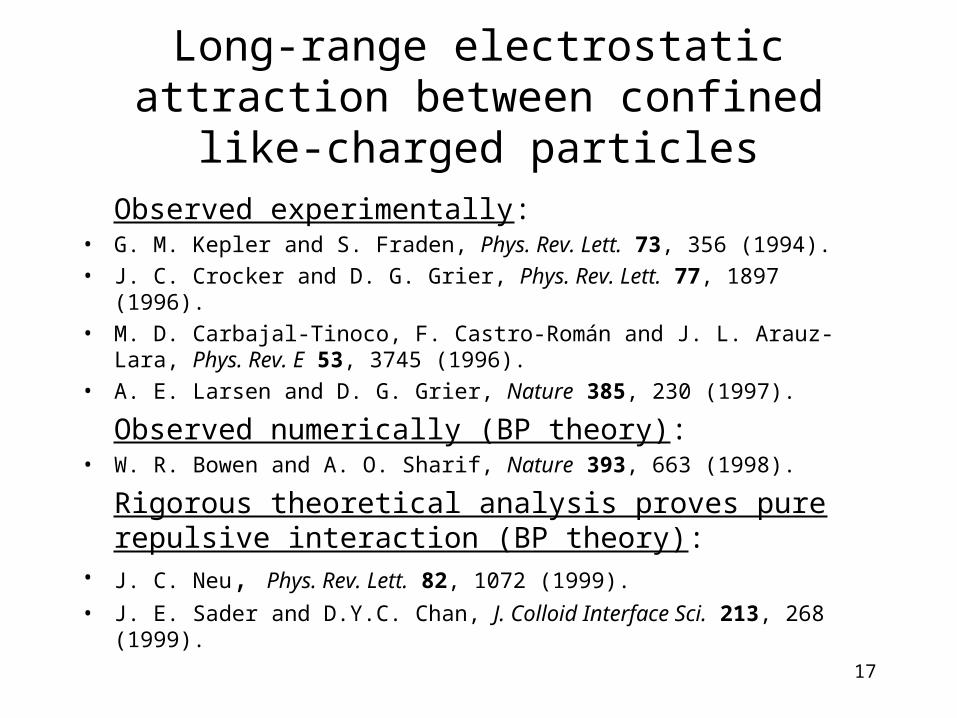
Long-range electrostatic attraction between confined like-charged particles

Observed experimentally:• G. M. Kepler and S. Fraden, Phys. Rev. Lett. 73, 356 (1994).

• J. C. Crocker and D. G. Grier, Phys. Rev. Lett. 77, 1897 (1996).

• M. D. Carbajal-Tinoco, F. Castro-Román and J. L. Arauz-Lara, Phys. Rev. E 53, 3745 (1996).

• A. E. Larsen and D. G. Grier, Nature 385, 230 (1997).

Observed numerically (BP theory):• W. R. Bowen and A. O. Sharif, Nature 393, 663 (1998).

Rigorous theoretical analysis proves pure repulsive interaction (BP theory):

• J. C. Neu, Phys. Rev. Lett. 82, 1072 (1999).

• J. E. Sader and D.Y.C. Chan, J. Colloid Interface Sci. 213, 268 (1999).

18

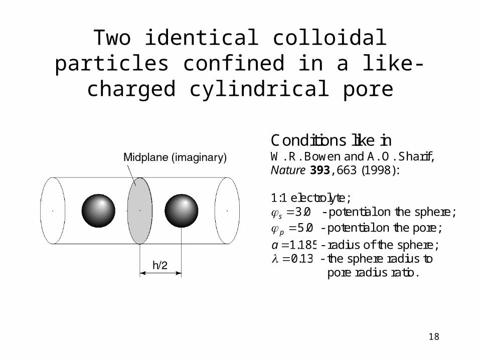
Two identical colloidal particles confined in a like-charged cylindrical pore

Conditions like in W. R. Bowen and A. O. Sharif, Nature 393, 663 (1998): 1:1 electrolyte;

0.3s - potential on the sphere; 0.5p - potential on the pore;

185.1a - radius of the sphere; 13.0 - the sphere radius to

pore radius ratio.

19

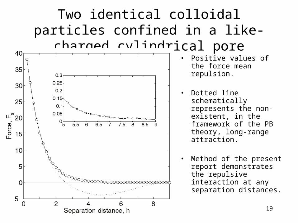
Two identical colloidal particles confined in a like-charged cylindrical pore

• Positive values of the force mean repulsion.

• Dotted line schematically represents the non-existent, in the framework of the PB theory, long-range attraction.

• Method of the present report demonstrates the repulsive interaction at any separation distances.

20

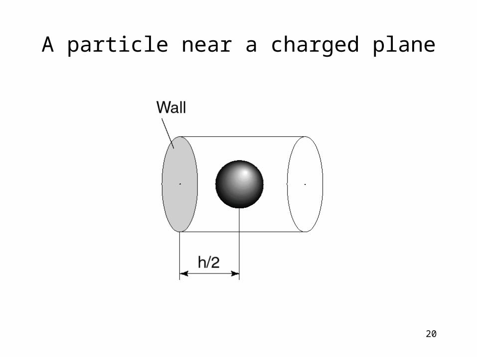
A particle near a charged plane

21

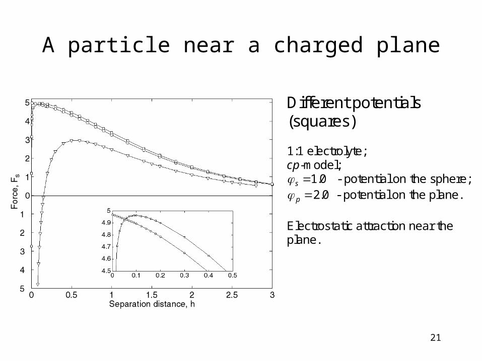
A particle near a charged plane

Different potentials (squares) 1:1 electrolyte; cp-model;

0.1s - potential on the sphere; 0.2p - potential on the plane.

Electrostatic attraction near the plane.

22

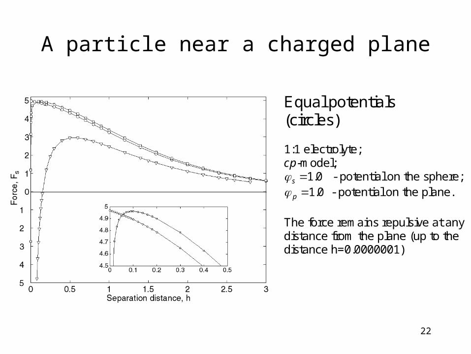
A particle near a charged plane

Equal potentials (circles) 1:1 electrolyte; cp-model;

0.1s - potential on the sphere; 0.1p - potential on the plane.

The force remains repulsive at any distance from the plane (up to the distance h=0.0000001)

23

Constant total charge model of a colloidal particle, ctc-model

• The total charge of the particle is kept constant.• The charge can move freely over the surface of the

particle.• Potential is uniform over the surface of the particle.

The difference between the ctc- and cp- models is that the total charge rather than the potential is kept constant.

24

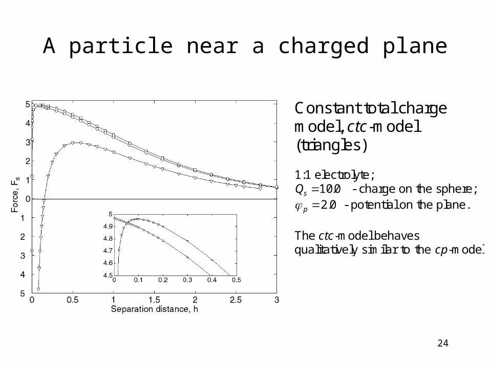
A particle near a charged plane

Constant total charge model, ctc-model (triangles) 1:1 electrolyte;

0.10sQ - charge on the sphere; 0.2p - potential on the plane.

The ctc-model behaves qualitatively similar to the cp-model.

25

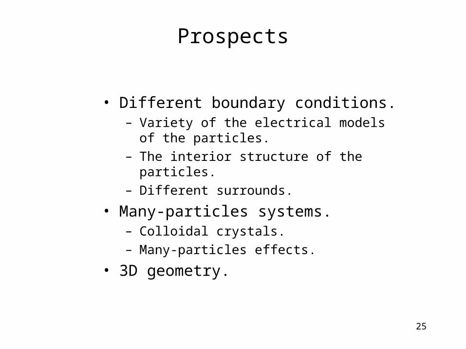
Prospects

• Different boundary conditions.– Variety of the electrical models of the

particles.– The interior structure of the particles.– Different surrounds.

• Many-particles systems.– Colloidal crystals.– Many-particles effects.

• 3D geometry.