Numerical modeling of magnetic induction and heating in ...orbit.dtu.dk/files/59842092/Numerical_modeling_of... · Numerical modeling of magnetic induction and ... main mechanisms

General rights Copyright and moral rights for the publications made accessible in the public portal are retained by the authors and/or other copyright owners and it is a condition of accessing publications that users recognise and abide by the legal requirements associated with these rights.

• Users may download and print one copy of any publication from the public portal for the purpose of private study or research. • You may not further distribute the material or use it for any profit-making activity or commercial gain • You may freely distribute the URL identifying the publication in the public portal

If you believe that this document breaches copyright please contact us providing details, and we will remove access to the work immediately and investigate your claim.

Downloaded from orbit.dtu.dk on: Jul 12, 2018

Numerical modeling of magnetic induction and heating in injection molding tools

Guerrier, Patrick; Hattel, Jesper Henri

Published in:Proceedings of International Conference on Advanced Manufacturing Engineering and Technologies(NEWTECH 2013)

Publication date:2013

Link back to DTU Orbit

Citation (APA):Guerrier, P., & Hattel, J. H. (2013). Numerical modeling of magnetic induction and heating in injection moldingtools. In Proceedings of International Conference on Advanced Manufacturing Engineering and Technologies(NEWTECH 2013) Kungl. Tekniska högskolan I Stockholm.

http://orbit.dtu.dk/en/publications/numerical-modeling-of-magnetic-induction-and-heating-in-injection-molding-tools(cd84290d-3b77-42b0-8c1f-ebc28fb2f0de).html

International Conference on Advanced Manufacturing Engineering and Technologies

Numerical modeling of magnetic induction and heating in

injection molding tools

Patrick Guerrier1, Jesper H. Hattel

1

1Technical University of Denmark, Department of Mechanical Engineering, Section of

Manufacturing Engineering, Denmark email [email protected]

ABSTRACT Injection molding of parts with special requirements or features such as micro-

or nanostructures on the surface, a good surface finish, or long and thin features

results in the need of a specialized technique to ensure proper filling and acceptable

cycle time. The aim of this study is to increase the temperatures as close as possible

to the cavity surface, by means of an integrated induction heating system in the

injection molding tool, to improve the fluidity of the polymer melt hereby ensuring

that the polymer melt will continue to flow until the mold cavity is completely filled.

The presented work uses numerical modeling of the induction heating in the mold to

investigate how the temperature in the mold will be distributed and how it is affected

by different material properties.

KEYWORDS: Induction heating, injection molding, finite element, coupled.

1. INRTRODUCTION

In order to injection mold special parts having micro- or nanostructures on the surface,

being long and having thin features, or requiring a good surface finish, elevated mold

temperatures will help ensuring complete filling of the cavity [1-3]. However, this can also

lead to an increased cycle time due to a longer cooling time, if the heating is not only done

locally where needed. The aim is therefore to only increase the temperature as close as

possible to the surface by means of an induction heating system to improve the fluidity of the

polymer melt hereby ensuring that the polymer melt will continue to flow until the mold

cavity is completely filled. The temperature required will depend on the transition temperature

of the polymer [1].

Recent studies [4-10] have been investigating induction heating of the mold tool, but

they are mainly focused on using an induction coil to heat up the surface of the mold before

the injection of the polymer. One drawback with this method is that a lot of the heat will

already be dissipated out into the mold and away from the surface. This will in turn not be

much warmer than without induction, as the whole mold will be heated up instead, again

leading to a longer cooling time.

mailto:[email protected]


The basic idea behind this new concept is that a coil should be placed beneath the mold

cavity surface, encased, on the backside, in a magnetic material, typically ferrite. The mold

cavity in front should be made of a non-magnetic material electroplated with a layer of

magnetic material e.g. nickel, to have the magnetic field running as close as possible to the

surface of the cavity side.

The presented work uses numerical modeling of the induction heating in the mold to

investigate the temperature distribution in the mold and especially at its surface. There are two

main mechanisms taking place in induction heating, namely electromagnetism and thermal

conduction. The electromagnetism is described by Maxwell’s equations which need to be

solved. A rapid changing magnetic field induces Eddy currents, which gives rise to a resistive

heating effect, known as Joule heating. The thermal conduction is controlled by the heat

conduction equation wherein the Joule heating is acting as a source term. The Eddy currents

tend to run at the surface of a magnetic conducting material due to the well-known effect of

the skin depth [11]. It is desired to find a combination of materials with different electrical

properties to get the heating as close as possible to the cavity surface. In this study different

material properties are investigated to find such a combination.

2. MECHANISMS

The electromagnetic part of induction heating is controlled by Maxwell’s equations,

which here are presented in terms of free charges and currents [12]:

f D (1)

0 B (2)

t

BE (3)

tf

DJH (4)

Where D is the electric flux density, B is the magnetic flux density, E is the electric

field, H is the magnetic field, fJ is the free current density, f is the free charge density, t

is the time. Relating D and H in terms of E and B depends on the material, and for linear

media it can be related through the following constitutive relations:

EED r0 (5)

BBHr0

11

(6)

Where 0 is the vacuum permittivity, r is the relative permittivity, 0 is the vacuum

permeability, and r is the relative permeability. Furthermore the current density and electric

field can be related by the well-known Ohm’s law:

EJ (7)


Where is the electrical conductivity. The displacement current in equation (4) will be

ignored and the assumption that a time-harmonic varying source current density will result in

a sinusoidally varying magnetic field will be made. Combining Maxwell’s equations (1)-(4)

with the constitutive equations (5)-(7), the following complex diffusion equation can be

derived [11]:

s2 i

1JAA

(8)

Where A is the magnetic vector potential related to the magnetic flux by AB ,

sJ is the source current density in the coil, f2 is the angular frequency (and f the

frequency), and the overbar is denoting the peak value or the amplitude. Assuming an

axisymmetric cylindrical system, the magnetic vector potential has an azimuthal component

only and equation (8) reduces to:

,s2

2

JAiz

A

r

Ar

rr

11 (9)

The magnetic flux can be found from the solution of the magnetic vector potential by

taking the curl of A , hence for the axisymmetric case it can be calculated as:

r

A

r

AB;

z

AB zr

(10)

The magnetic field can then be found using equation (6). The induced Eddy currents in

the conductors can be found from:

AiJe (11)

From which the Joule heating can be found via:

2

e21 JQ

(12)

Which is the volumetric heat source induced by the Eddy currents. A well-known and

useful expression is the current skin depth or penetration depth, which can also be derived

from Maxwell’s equations. This quantity is defined as the distance for which the amplitude of

a plane wave decreases by a factor of 368.01 e , and will prove useful later:

f

1 (13)

The other mechanism taking place in induction heating is the heat conduction, which can

be described by the transient heat conduction equation:


QTkt

Tc 2

p

(14)

Where T is the temperature, is the density, pc is the specific heat capacity, k is the

thermal conductivity, and Q is the heat source from equation (12).

3. FINITE ELEMENT FORMULATION

The finite element method has been used to solve equation (9) and (14). This implies

first finding the heat source term from the electromagnetic solution and then using it in the

transient heat conduction equation to get the resulting temperature distribution. The

implementation of the finite element formulation is done in-house and is self-developed using

MATLAB. The implementation is tested against the commercial software COMSOL and

QuickField, to validate the code. For the actual experimental setup presented here, it was

chosen to use the self-developed implementation due to its code flexibility and fast solution

time. Using the Galerkin method to approximate the solution on a set of discrete points we get

0JAiz

A

r

Ar

rr

11N ,s2

2T

d (15)

where N is a row vector containing the shape functions, and is the domain of

interest. The total matrix system becomes:

fACiK (16)

with the following element matrix equations:

dBBKT1

e ;

dNNCT

e ;

dT

NJf se (17)

where B is the derivative of the shape function also called gradient matrix. Linear

triangular elements have been employed and a closed form solution of the integration has been

done with the resulting elemental matrices being similar to those described in [11].

The heat conduction equation is discretized in a similar way. Employing equation (14) in

cylindrical coordinates and using the Galerkin method we obtain

0t

TcQ

z

T

r

Tr

rr

1kN p2

2T

d (18)

Inserting the spatial approximation of the temperature will then result in the following

form of matrix equation:


fTKt

TC

(19)

With similar element matrices to those in equation (17) but substituting 1 with k ,

with pc , and sJ with Q . The time derivative is discretized using an implicit Euler

approximation (backward finite difference) to yield the following form:

ftTCTKtCn1n

(20)

Where t is the time step. The implicit formulation has the advantage of being

unconditionally stable. Both equation systems seen in equation (16) and (20) are built as

sparse matrices and both are solved using MATLAB’s build-in solver, which can solve

unsymmetrical sparse linear systems on the form bxA .

4. GEOMETRICAL SETUP

An induction heating setup has been employed with the self-developed finite element

code and in COMSOL. Only the results from the self-developed code will be shown as they

are identical to the COMSOL implementation. This is done to investigate the temperature

distribution in the mold utilizing a unique combination of materials to get the Eddy currents as

close as possible to the mold cavity. All components have been integrated into the mold itself,

in order to avoid external inductors to heat the mold surface. Also, the unit can be used with a

conventional injection molding machine, with the only extra equipment being the power

supply.

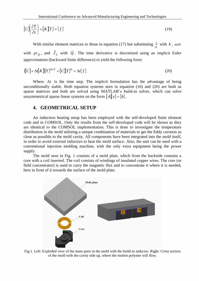
The mold seen in Fig. 1 consists of a mold plate, which from the backside contains a

core with a coil inserted. The coil consists of windings of insulated copper wires. The core (or

field concentrator) is used to carry the magnetic flux and to concentrate it where it is needed,

here in front of it towards the surface of the mold plate.

Fig.1. Left: Exploded view of the main parts in the mold with the build-in inductor. Right: Cross section

of the mold with the cavity side up, where the molten polymer will flow.


5. NUMERICAL MODEL SETUP

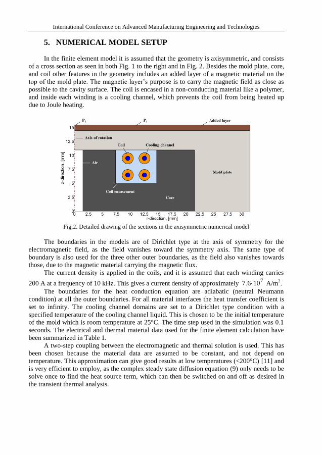
In the finite element model it is assumed that the geometry is axisymmetric, and consists

of a cross section as seen in both Fig. 1 to the right and in Fig. 2. Besides the mold plate, core,

and coil other features in the geometry includes an added layer of a magnetic material on the

top of the mold plate. The magnetic layer’s purpose is to carry the magnetic field as close as

possible to the cavity surface. The coil is encased in a non-conducting material like a polymer,

and inside each winding is a cooling channel, which prevents the coil from being heated up

due to Joule heating.

Fig.2. Detailed drawing of the sections in the axisymmetric numerical model

The boundaries in the models are of Dirichlet type at the axis of symmetry for the

electromagnetic field, as the field vanishes toward the symmetry axis. The same type of

boundary is also used for the three other outer boundaries, as the field also vanishes towards

those, due to the magnetic material carrying the magnetic flux.

The current density is applied in the coils, and it is assumed that each winding carries

200 A at a frequency of 10 kHz. This gives a current density of approximately 7107.6 A/m

2.

The boundaries for the heat conduction equation are adiabatic (neutral Neumann

condition) at all the outer boundaries. For all material interfaces the heat transfer coefficient is

set to infinity. The cooling channel domains are set to a Dirichlet type condition with a

specified temperature of the cooling channel liquid. This is chosen to be the initial temperature

of the mold which is room temperature at 25°C. The time step used in the simulation was 0.1

seconds. The electrical and thermal material data used for the finite element calculation have

been summarized in Table 1.

A two-step coupling between the electromagnetic and thermal solution is used. This has

been chosen because the material data are assumed to be constant, and not depend on

temperature. This approximation can give good results at low temperatures (<200°C) [11] and

is very efficient to employ, as the complex steady state diffusion equation (9) only needs to be

solve once to find the heat source term, which can then be switched on and off as desired in

the transient thermal analysis.


Table 1. Electromagnetic and thermal properties used for the different materials (sections)

Material Relative

permea-

Bility [-]

Electrical

conductivity

[S/m]

Thermal

conductivity

[W/mK]

Density

[kg/m3]

Specific heat

capacity

[J/kgK]

Air 1 0 0.0257 1.205 1.005

Copper (Coil) 1 6e7 400 8700 385

Ferromagnetic

ceramic (Core) 600 100 4 5000 700

Non-magnetic

Steel (Mold) 1 1.45e6 28 7750 460

Nickel (Layer) 100 1.43e7 91 8900 460

Silicone (Enca.) 1 3.16e-12 0.3 1550 1200

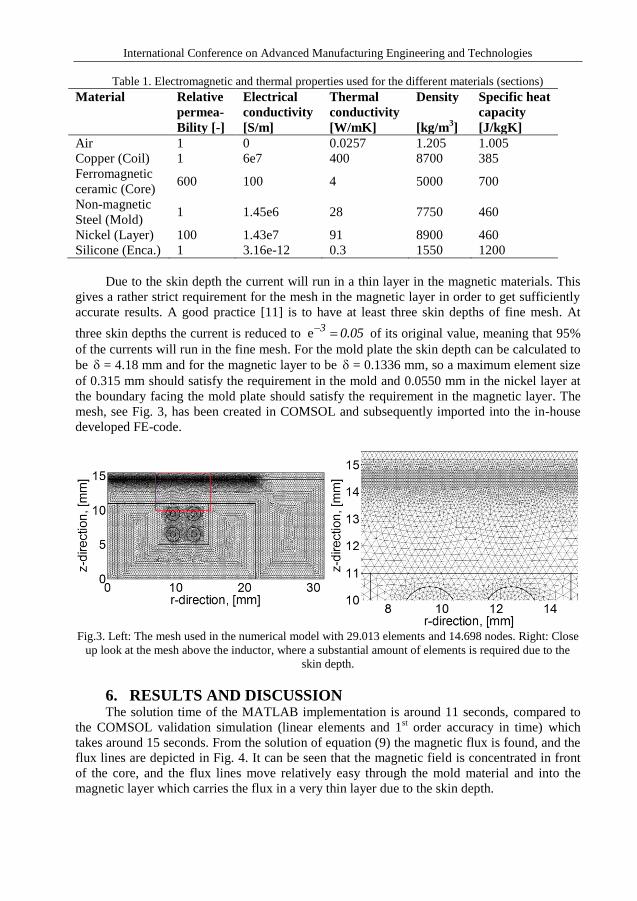
Due to the skin depth the current will run in a thin layer in the magnetic materials. This

gives a rather strict requirement for the mesh in the magnetic layer in order to get sufficiently

accurate results. A good practice [11] is to have at least three skin depths of fine mesh. At

three skin depths the current is reduced to 05.03 e of its original value, meaning that 95%

of the currents will run in the fine mesh. For the mold plate the skin depth can be calculated to

be = 4.18 mm and for the magnetic layer to be = 0.1336 mm, so a maximum element size

of 0.315 mm should satisfy the requirement in the mold and 0.0550 mm in the nickel layer at

the boundary facing the mold plate should satisfy the requirement in the magnetic layer. The

mesh, see Fig. 3, has been created in COMSOL and subsequently imported into the in-house

developed FE-code.

Fig.3. Left: The mesh used in the numerical model with 29.013 elements and 14.698 nodes. Right: Close

up look at the mesh above the inductor, where a substantial amount of elements is required due to the

skin depth.

6. RESULTS AND DISCUSSION The solution time of the MATLAB implementation is around 11 seconds, compared to

the COMSOL validation simulation (linear elements and 1st order accuracy in time) which

takes around 15 seconds. From the solution of equation (9) the magnetic flux is found, and the

flux lines are depicted in Fig. 4. It can be seen that the magnetic field is concentrated in front

of the core, and the flux lines move relatively easy through the mold material and into the

magnetic layer which carries the flux in a very thin layer due to the skin depth.


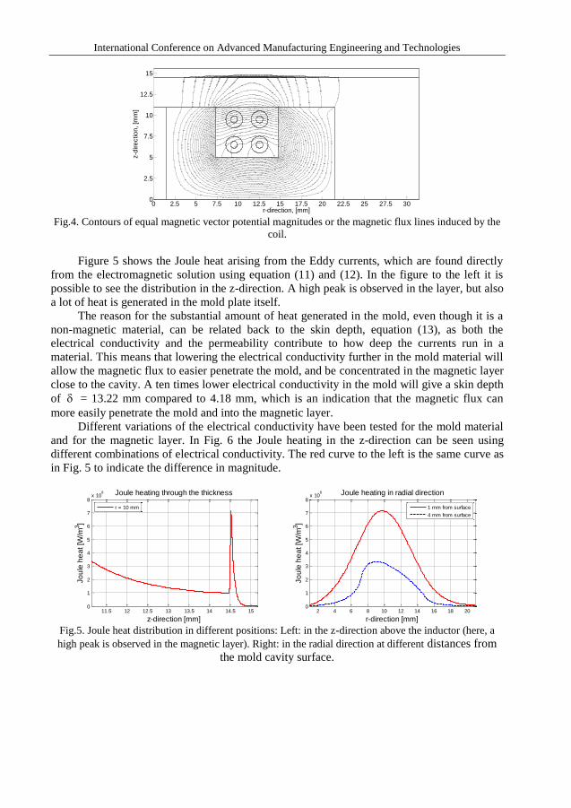
Fig.4. Contours of equal magnetic vector potential magnitudes or the magnetic flux lines induced by the

coil.

Figure 5 shows the Joule heat arising from the Eddy currents, which are found directly

from the electromagnetic solution using equation (11) and (12). In the figure to the left it is

possible to see the distribution in the z-direction. A high peak is observed in the layer, but also

a lot of heat is generated in the mold plate itself.

The reason for the substantial amount of heat generated in the mold, even though it is a

non-magnetic material, can be related back to the skin depth, equation (13), as both the

electrical conductivity and the permeability contribute to how deep the currents run in a

material. This means that lowering the electrical conductivity further in the mold material will

allow the magnetic flux to easier penetrate the mold, and be concentrated in the magnetic layer

close to the cavity. A ten times lower electrical conductivity in the mold will give a skin depth

of = 13.22 mm compared to 4.18 mm, which is an indication that the magnetic flux can

more easily penetrate the mold and into the magnetic layer.

Different variations of the electrical conductivity have been tested for the mold material

and for the magnetic layer. In Fig. 6 the Joule heating in the z-direction can be seen using

different combinations of electrical conductivity. The red curve to the left is the same curve as

in Fig. 5 to indicate the difference in magnitude.

Fig.5. Joule heat distribution in different positions: Left: in the z-direction above the inductor (here, a

high peak is observed in the magnetic layer). Right: in the radial direction at different distances from

the mold cavity surface.

0 2.5 5 7.5 10 12.5 15 17.5 20 22.5 25 27.5 300

2.5

5

7.5

10

12.5

15

r-direction, [mm]

z-d

ire

ctio

n, [m

m]

11.5 12 12.5 13 13.5 14 14.5 150

1

2

3

4

5

6

7

8x 10

8 Joule heating through the thickness

z-direction [mm]

Jo

ule

he

at [W

/m3]

r = 10 mm

2 4 6 8 10 12 14 16 18 200

1

2

3

4

5

6

7

8x 10

8 Joule heating in radial direction

r-direction [mm]

Jo

ule

he

at [W

/m3]

1 mm from surface

4 mm from surface


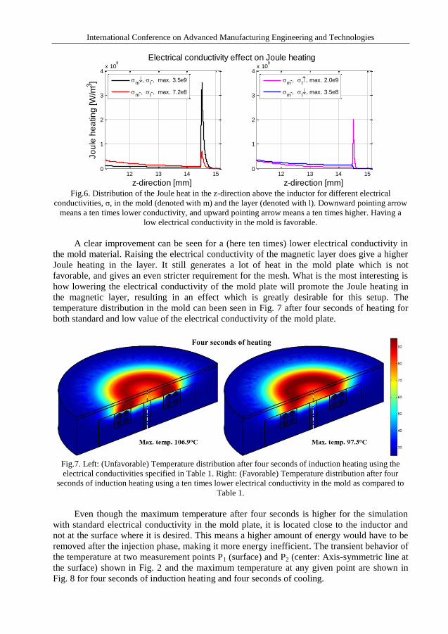
Fig.6. Distribution of the Joule heat in the z-direction above the inductor for different electrical

conductivities, σ, in the mold (denoted with m) and the layer (denoted with l). Downward pointing arrow

means a ten times lower conductivity, and upward pointing arrow means a ten times higher. Having a

low electrical conductivity in the mold is favorable.

A clear improvement can be seen for a (here ten times) lower electrical conductivity in

the mold material. Raising the electrical conductivity of the magnetic layer does give a higher

Joule heating in the layer. It still generates a lot of heat in the mold plate which is not

favorable, and gives an even stricter requirement for the mesh. What is the most interesting is

how lowering the electrical conductivity of the mold plate will promote the Joule heating in

the magnetic layer, resulting in an effect which is greatly desirable for this setup. The

temperature distribution in the mold can been seen in Fig. 7 after four seconds of heating for

both standard and low value of the electrical conductivity of the mold plate.

Fig.7. Left: (Unfavorable) Temperature distribution after four seconds of induction heating using the

electrical conductivities specified in Table 1. Right: (Favorable) Temperature distribution after four

seconds of induction heating using a ten times lower electrical conductivity in the mold as compared to

Table 1.

Even though the maximum temperature after four seconds is higher for the simulation

with standard electrical conductivity in the mold plate, it is located close to the inductor and

not at the surface where it is desired. This means a higher amount of energy would have to be

removed after the injection phase, making it more energy inefficient. The transient behavior of

the temperature at two measurement points P1 (surface) and P2 (center: Axis-symmetric line at

the surface) shown in Fig. 2 and the maximum temperature at any given point are shown in

Fig. 8 for four seconds of induction heating and four seconds of cooling.

12 13 14 150

1

2

3

4x 10

9

z-direction [mm]

Jo

ule

he

atin

g [W

/m3]

m,

l-, max. 3.5e9

m

-, l-, max. 7.2e8

12 13 14 150

1

2

3

4x 10

9

z-direction [mm]

m

-, l, max. 2.0e9

m

-, l, max. 3.5e8

Electrical conductivity effect on Joule heating


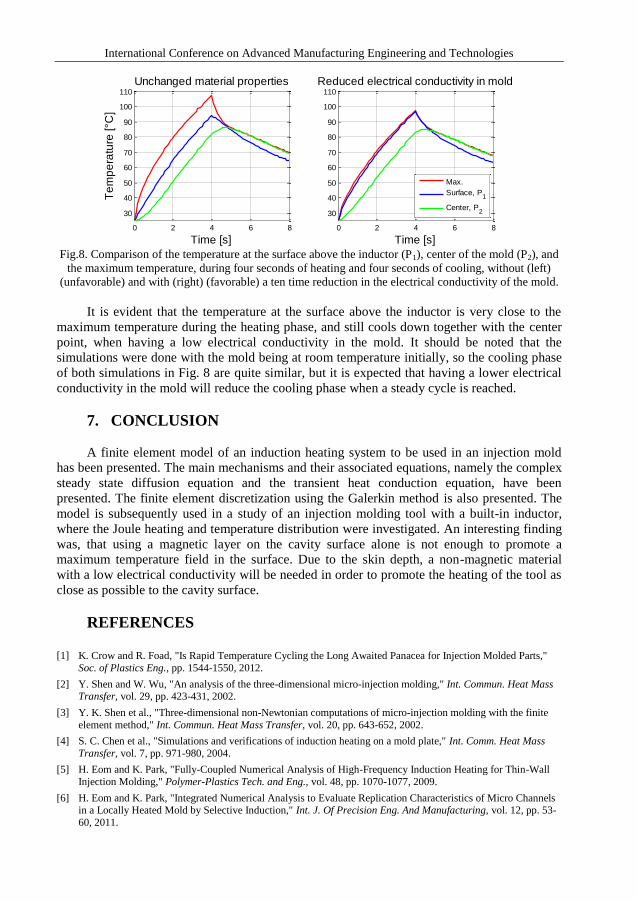
Fig.8. Comparison of the temperature at the surface above the inductor (P1), center of the mold (P2), and

the maximum temperature, during four seconds of heating and four seconds of cooling, without (left)

(unfavorable) and with (right) (favorable) a ten time reduction in the electrical conductivity of the mold.

It is evident that the temperature at the surface above the inductor is very close to the

maximum temperature during the heating phase, and still cools down together with the center

point, when having a low electrical conductivity in the mold. It should be noted that the

simulations were done with the mold being at room temperature initially, so the cooling phase

of both simulations in Fig. 8 are quite similar, but it is expected that having a lower electrical

conductivity in the mold will reduce the cooling phase when a steady cycle is reached.

7. CONCLUSION

A finite element model of an induction heating system to be used in an injection mold

has been presented. The main mechanisms and their associated equations, namely the complex

steady state diffusion equation and the transient heat conduction equation, have been

presented. The finite element discretization using the Galerkin method is also presented. The

model is subsequently used in a study of an injection molding tool with a built-in inductor,

where the Joule heating and temperature distribution were investigated. An interesting finding

was, that using a magnetic layer on the cavity surface alone is not enough to promote a

maximum temperature field in the surface. Due to the skin depth, a non-magnetic material

with a low electrical conductivity will be needed in order to promote the heating of the tool as

close as possible to the cavity surface.

REFERENCES

[1] K. Crow and R. Foad, "Is Rapid Temperature Cycling the Long Awaited Panacea for Injection Molded Parts,"

Soc. of Plastics Eng., pp. 1544-1550, 2012.

[2] Y. Shen and W. Wu, "An analysis of the three-dimensional micro-injection molding," Int. Commun. Heat Mass Transfer, vol. 29, pp. 423-431, 2002.

[3] Y. K. Shen et al., "Three-dimensional non-Newtonian computations of micro-injection molding with the finite

element method," Int. Commun. Heat Mass Transfer, vol. 20, pp. 643-652, 2002.

[4] S. C. Chen et al., "Simulations and verifications of induction heating on a mold plate," Int. Comm. Heat Mass

Transfer, vol. 7, pp. 971-980, 2004.

[5] H. Eom and K. Park, "Fully-Coupled Numerical Analysis of High-Frequency Induction Heating for Thin-Wall

Injection Molding," Polymer-Plastics Tech. and Eng., vol. 48, pp. 1070-1077, 2009.

[6] H. Eom and K. Park, "Integrated Numerical Analysis to Evaluate Replication Characteristics of Micro Channels in a Locally Heated Mold by Selective Induction," Int. J. Of Precision Eng. And Manufacturing, vol. 12, pp. 53-

60, 2011.

0 2 4 6 8

30

40

50

60

70

80

90

100

110

Unchanged material properties

Time [s]

Te

mp

era

ture

[°C

]

0 2 4 6 8

30

40

50

60

70

80

90

100

110

Time [s]

Reduced electrical conductivity in mold

Max.

Surface, P1

Center, P2


[7] M.-S. Huang et al., "Electromagnetic Induction Coil Design for Mold Surface," Soc. of Plastics Eng., pp. 1471-

1476, 2012.

[8] H.-L. Lin et al., "Induction heating with the ring effect for injection molding plates," Int. Commun. in Heat and

Mass Transfer, vol. 39, pp. 514-522, 2012.

[9] K. Park and S.-I. Lee, "Localized mold heating with the aid of selective induction for injection molding of high aspect ratio micro-features," J. Of Micromechanics And Microengineering, vol. 20, pp. 1-11, 2010.

[10] Y.-T. Sung et al., "Design of Induction Heating Module for Uniform Cavity," Soc. of Plastics Eng., pp. 1427-

1436, 2012.

[11] V. Rudnec et al., Handbook of Induction Heating, Marcel Dekker, Inc., 2003.

[12] D. J. Griffiths, Introduction to Electrodynamics, Prentice Hall, 1999.

Documents

Numerical modeling of magnetic induction and heating in ...orbit.dtu.dk/files/59842092/Numerical_modeling_of... · Numerical modeling of magnetic induction and ... main mechanisms