Received May 1, 2019, accepted May 20, 2019, date of publication May 27, 2019, date of current version June 10, 2019.

Digital Object Identifier 10.1109/ACCESS.2019.2919140

Magnetic Induction Tomography Using MagneticDipole and Lumped Parameter ModelJIYUN JEON , WONMO CHUNG , AND HUNGSUN SON , (Member, IEEE)Ulsan National Institute of Science and Technology, Ulsan 44919, South Korea

Corresponding author: Hungsun Son (hson@unist.ac.kr)

This work was supported in part by the Ulsan National Institute of Science and Technology (UNIST) through the Future InnovationResearch Funds under Grant 1.190011.01, in part by the Development of Multi-Degrees Of Freedom Spherical Motion Platform underGrant 2.190080.01, and in part by the Development of Drone System for Ship and Marine Mission of Civil Military TechnologyCooperation Center under Grant 2.180832.01.

ABSTRACT This paper presents a novel approach to analyze the magnetic field of magnetic inductiontomography (MIT) using magnetic dipoles and a lumped parameter model. The MIT is a next-generationmedical imaging technique that can identify the conductivity of target objects and construct images. It isnoninvasive and can be compact in design and, thus, used as a portable instrument. However, it still exhibitsinferior performance due to the nonlinearity, low signal-to-noise ratio of the magnetic field, and ill-posedinverse problem. To overcome such difficulties, the magnetic field of the MIT system is first modeledusing magnetic dipoles and a lumped parameter. In particular, the extended distributed multipole (eDMP)model is proposed to analyze the system, using magnetic dipoles. The method can dramatically reduce thecomputational efforts and improve the ill-posed condition. Hence, the forward and inverse problems of MITare solved using the eDMP method. The modeling method can be validated by comparing with experiments,varying the modeling parameters. Finally, the image can be reconstructed, and then, the position and shapeof the object can be characterized to develop the MIT.

INDEX TERMS Extended distributed multipole (eDMP), equivalent circuit modeling, magnetic dipolemodeling, magnetic induction tomography (MIT), time-varying magnetic field, eddy current model.

I. INTRODUCTIONMagnetic induction tomography (MIT) is a medical imag-ing device that uses electromagnetic properties, such asconductivity, to characterize a target object. The exist-ing imaging devices, such as X-ray, CT, and MRI, havebeen in use for several decades. However, the instrumentsused in these devices are large and incur high power andcost. In addition, an expert is required to operate thedevices, as they can be harmful. In contrast, MIT incurslow power and cost, and thus, is portable and can beused during emergency. In addition, owing to its noninva-sive and harmless properties, experts are not required foroperation.

AMIT system comprises numerous transmitter coils (Txs)and receiver coils (Rxs). Unknown conductive objects areplaced in a region of interest (ROI) and cause magneticperturbation, as Txs are activated. The perturbation is shown

The associate editor coordinating the review of this manuscript andapproving it for publication was Kezhi Li.

as phase shift at Rxs and analyzed to reconstruct an image.The principle has been utilized in the industry to detect themetal crack for a hundred years [1]. However, as humantissues are extremely low conductivity materials (< 5 S/m),the signal-to-noise ratio (SNR) is also low. Thus, researchershave been trying to improve the performance of MIT sinceearly 90s [2]. Various designs and arrangements of Txs andRxs have been attempted: multichannel Rxs, changing ori-entation [3]; hemispherical array [4]; and planar array [5].In addition, there have been attempts to change the coil typeof an Rx, not only a voice coil but also planar coil [6], gra-diometer [7]–[9], atomic magnetometer [10], superconduct-ing quantum interference device (SQUID) [1]. To enhanceSNR, shielding Txs and Rxs from noise and inserting aniron core into Txs are suggested in [11]. As the conductivityof human tissues depends on frequency, a multifrequencyinput has been applied to identify the function [4], [8], [12].Target objects have also been examined from the salinewater [13] and agarose [14] administered to rats [15] andrabbits [16], [17]. It is also applied to detect metal for the

VOLUME 7, 20192169-3536 2019 IEEE. Translations and content mining are permitted for academic research only.

Personal use is also permitted, but republication/redistribution requires IEEE permission.See http://www.ieee.org/publications_standards/publications/rights/index.html for more information.

70287

J. Jeon et al.: MIT Using Magnetic Dipole and Lumped Parameter Model

industrial applications, such as steel and alloy [18], [19].MIT can be combined with existing techniques, such asmagneto-acousto-electrical tomography [20] and holographytechnique [21].

So far, various designs of an MIT system have been devel-oped, but it still shows inferior performance because themagnetic field is intrinsically weak and the analysis of thefield is nonlinear and rather complicated. Thus, numericalmethods have been utilized to analyze the magnetic fieldand design MIT systems for high accuracy [22]–[24]. How-ever, the method requires heavy computational effort andcontributes to increasing the system volume. Thus, a novelapproach demanding fast computation and high accuracyis required to achieve a MIT system. A lumped parame-ter method is applied to identify and control the systemin real time with first-order accuracy. The equivalent cir-cuit model can identify eddy current distribution, and itsinteraction in tissues [25], [26]. However, this method facesdifficulty in describing the detailed characters of the sys-tem, such as positions and orientations of Txs and Rxs.Thus, various methods are used to supplement the draw-back. For example, in [25], an analytic method computesthe induced voltage, and in [26], a numerical method solvesthe forward problem of MIT. However, combining the ana-lytic and numerical method still requires high computationalresource.

The magnetic dipole moment model can analyze the time-varying magnetic field in real time considering the geometryof the system components. The magnetic single-dipole (SD)model is applied to compute the magnetic far-field accurately.The extended distributed multipole (eDMP) method has beenproposed to enhance accuracy in the near-field and computethe interaction between magnetic fields, such as magneticinduction, Lorentz force, and torque fast [27]–[29]. In thisstudy, the eDMP method is applied to supplement the equiv-alent circuit model. The equivalent circuit modeling is appliedto identify an entire system of the MIT using Z-parameters.Then, the eDMP can estimate the Z-parameters, consideringthe properties of the objects and system setup. Once forwardmodeling is constructed, an inverse algorithm can be devel-oped. Then, conductivity in the ROI can be determined bysolving the inverse of phase shift and image processing canbe achieved.

The experiments are performed to demonstrate the methodis applicable to a MIT system. The object with uniformconductivity is applied as illustration and the effect of theobject properties is studied since it requires high sensitivityfor variation in the properties.

The remainder of this paper is organized as follows:First, the eDMP model and the equivalent circuit model areapplied to modeling MIT. The modeling method is com-pared with experiments and other simulation method vary-ing the object properties for validation. Then, the imageis reconstructed to characterize the object in the ROI. Theresults can estimate the applicability of the eDMP methodto MIT.

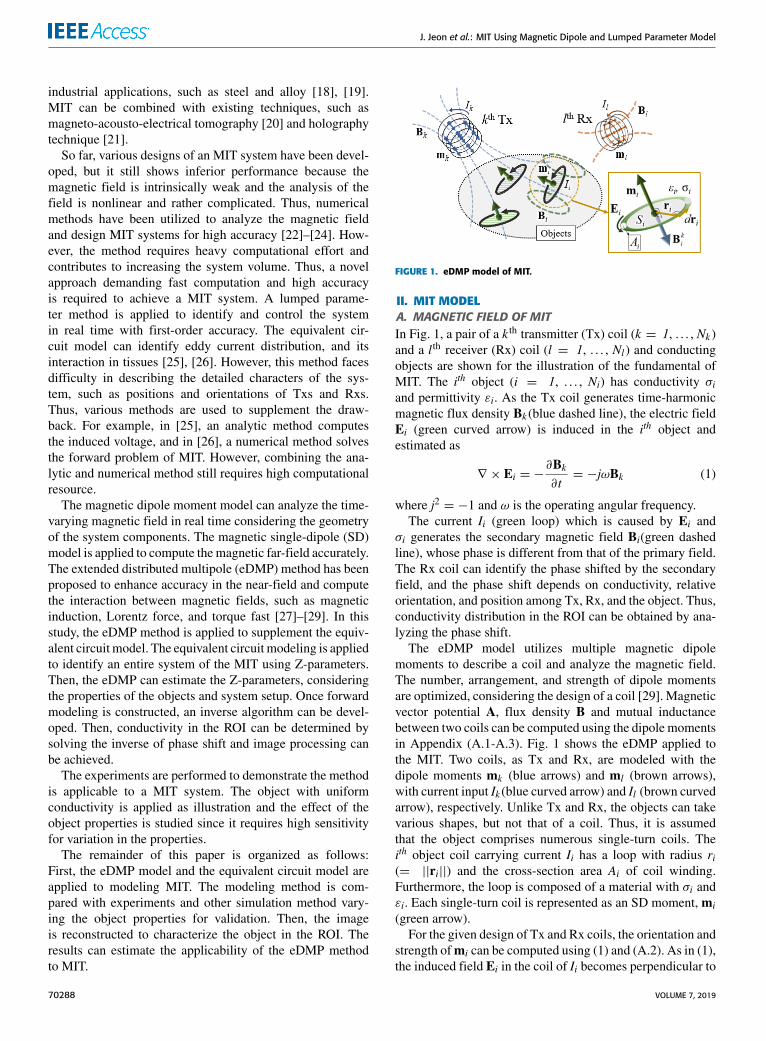
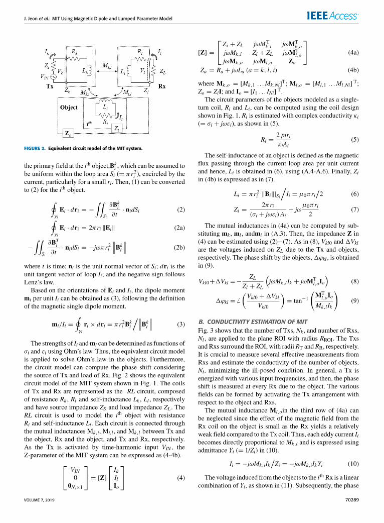
FIGURE 1. eDMP model of MIT.

II. MIT MODELA. MAGNETIC FIELD OF MITIn Fig. 1, a pair of a k th transmitter (Tx) coil (k = 1, . . . , Nk )and a l th receiver (Rx) coil (l = 1, . . . , Nl) and conductingobjects are shown for the illustration of the fundamental ofMIT. The ith object (i = 1, . . . , Ni) has conductivity σiand permittivity εi. As the Tx coil generates time-harmonicmagnetic flux density Bk (blue dashed line), the electric fieldEi (green curved arrow) is induced in the ith object andestimated as

∇ × Ei = −∂Bk∂t= −jωBk (1)

where j2 = −1 and ω is the operating angular frequency.The current Ii (green loop) which is caused by Ei and

σi generates the secondary magnetic field Bi(green dashedline), whose phase is different from that of the primary field.The Rx coil can identify the phase shifted by the secondaryfield, and the phase shift depends on conductivity, relativeorientation, and position among Tx, Rx, and the object. Thus,conductivity distribution in the ROI can be obtained by ana-lyzing the phase shift.

The eDMP model utilizes multiple magnetic dipolemoments to describe a coil and analyze the magnetic field.The number, arrangement, and strength of dipole momentsare optimized, considering the design of a coil [29]. Magneticvector potential A, flux density B and mutual inductancebetween two coils can be computed using the dipole momentsin Appendix (A.1-A.3). Fig. 1 shows the eDMP applied tothe MIT. Two coils, as Tx and Rx, are modeled with thedipole moments mk (blue arrows) and ml (brown arrows),with current input Ik (blue curved arrow) and Il (brown curvedarrow), respectively. Unlike Tx and Rx, the objects can takevarious shapes, but not that of a coil. Thus, it is assumedthat the object comprises numerous single-turn coils. Theith object coil carrying current Ii has a loop with radius ri(= ||ri||) and the cross-section area Ai of coil winding.Furthermore, the loop is composed of a material with σi andεi. Each single-turn coil is represented as an SD moment,mi(green arrow).

For the given design of Tx and Rx coils, the orientation andstrength ofmi can be computed using (1) and (A.2). As in (1),the induced field Ei in the coil of Ii becomes perpendicular to

70288 VOLUME 7, 2019

J. Jeon et al.: MIT Using Magnetic Dipole and Lumped Parameter Model

FIGURE 2. Equivalent circuit model of the MIT system.

the primary field at the ith object,Bki , which can be assumed tobe uniform within the loop area Si (= πr2i ), encircled by thecurrent, particularly for a small ri. Then, (1) can be convertedto (2) for the ith object.∮

γi

Ei · dri = −∫∫

Si

∂Bki∂t· nidSi (2)∮

γi

Ei · dri = 2πri ‖Ei‖ (2a)

−

∫∫Si

∂BTi∂t· nidSi = −jωπr2i

∥∥∥Bki ∥∥∥ (2b)

where t is time; ni is the unit normal vector of Si; dri is theunit tangent vector of loop Ii; and the negative sign followsLenz’s law.

Based on the orientations of Ei and Ii, the dipole momentmi per unit Ii can be obtained as (3), following the definitionof the magnetic single dipole moment.

mi/Ii =∮γi

ri × dri = πr2i Bki

/∥∥∥Bki ∥∥∥ (3)

The strengths of Ii andmi can be determined as functions ofσi and εi using Ohm’s law. Thus, the equivalent circuit modelis applied to solve Ohm’s law in the objects. Furthermore,the circuit model can compute the phase shift consideringthe source of Tx and load of Rx. Fig. 2 shows the equivalentcircuit model of the MIT system shown in Fig. 1. The coilsof Tx and Rx are represented as the RL circuit, composedof resistance Rk , Rl and self-inductance Lk , Ll , respectivelyand have source impedance ZS and load impedance ZL . TheRL circuit is used to model the ith object with resistanceRi and self-inductance Li. Each circuit is connected throughthe mutual inductances Mk,i, Mi,l , and Mk,l between Tx andthe object, Rx and the object, and Tx and Rx, respectively.As the Tx is activated by time-harmonic input VIN , theZ-parameter of the MIT system can be expressed as (4-4b). VIN

00Ni×1

= [Z]

IkIlIo

(4)

[Z] =

Zs + Zk jωMTk,l jωMT

k,ojωMk,l Zl + ZL jωMT

l,ojωMk,o jωMl,o Zo

(4a)

Za = Ra + jωLa (a = k, l, i) (4b)

where Mk,o = [Mk,1 . . .Mk,Ni]T; Ml,o = [Ml,1 . . .Ml,Ni] T;Zo = ZiI; and Io = [I1 . . . INi] T.The circuit parameters of the objects modeled as a single-

turn coil, Ri and Li, can be computed using the coil designshown in Fig. 1. Ri is estimated with complex conductivity κi(= σi + jωεi), as shown in (5).

Ri =2 piriκiAi

(5)

The self-inductance of an object is defined as the magneticflux passing through the current loop area per unit currentand hence, Li is obtained in (6), using (A.4-A.6). Finally, Ziin (4b) is expressed as in (7).

Li = πr2i ‖Bi‖|Si/Ii = µ0πri

/2 (6)

Zi =2πri

(σi + jωεi)Ai+ jω

µ0πri2

(7)

The mutual inductances in (4a) can be computed by sub-stituting mk , ml , andmi in (A.3). Then, the impedance Z in(4) can be estimated using (2)−(7). As in (8), Vkl0 and 1Vklare the voltages induced on ZL due to the Tx and objects,respectively. The phase shift by the objects,1ϕkl , is obtainedin (9).

Vkl0+1Vkl =−ZL

Zl + ZL

(jωMk,lIk + jωMT

l,oIo)

(8)

1ϕkl = 6

(Vkl0 +1Vkl

Vkl0

)= tan−1

(MT

l,oIoMk,lIk

)(9)

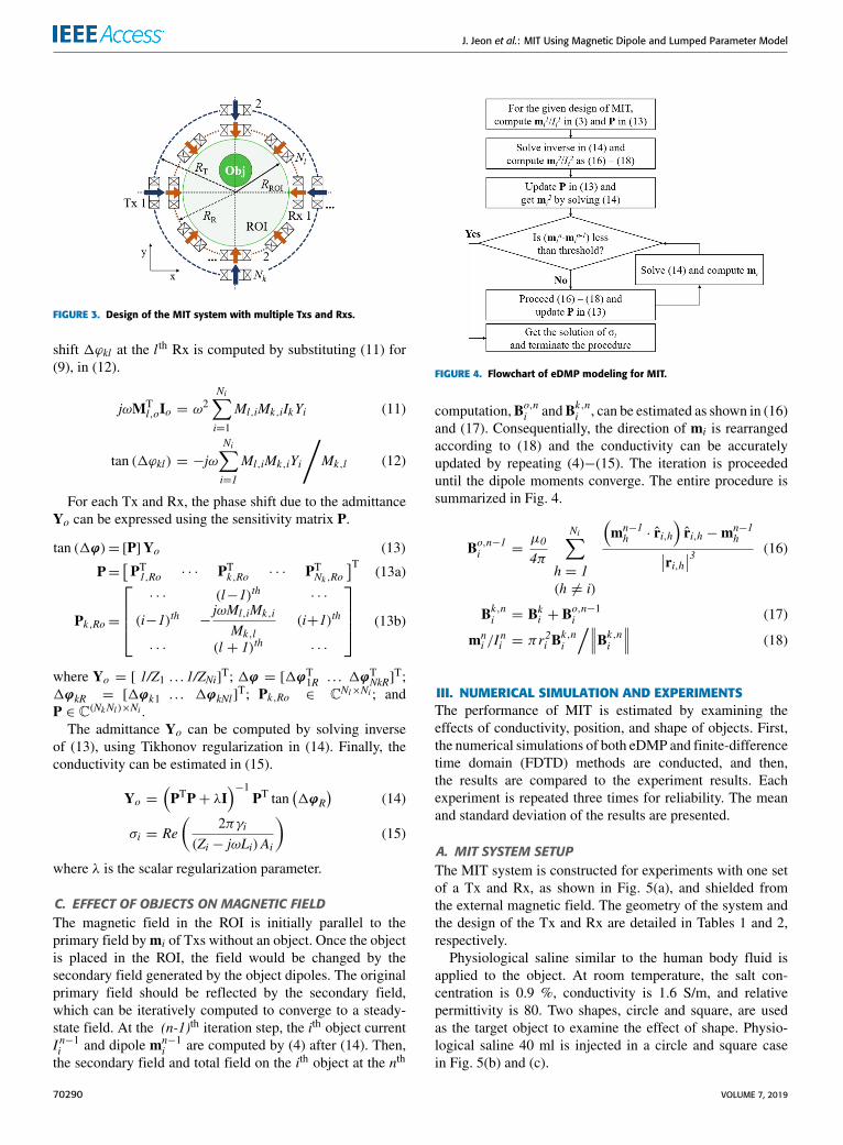
B. CONDUCTIVITY ESTIMATION OF MITFig. 3 shows that the number of Txs, Nk , and number of Rxs,Nl , are applied to the plane ROI with radius RROI. The Txsand Rxs surround the ROI, with radii RT and RR, respectively.It is crucial to measure several effective measurements fromRxs and estimate the conductivity of the number of objects,Ni, minimizing the ill-posed condition. In general, a Tx isenergized with various input frequencies, and then, the phaseshift is measured at every Rx due to the object. The variousfields can be formed by activating the Tx arrangement withrespect to the object and Rxs.

The mutual inductance Ml,oin the third row of (4a) canbe neglected since the effect of the magnetic field from theRx coil on the object is small as the Rx yields a relativelyweak field compared to the Tx coil. Thus, each eddy current Iibecomes directly proportional toMk,i and is expressed usingadmittance Yi (= 1/Zi) in (10).

Ii = −jωMk,iIk/Zi = −jωMk,iIkYi (10)

The voltage induced from the objects to the l th Rx is a linearcombination of Yi, as shown in (11). Subsequently, the phase

VOLUME 7, 2019 70289

J. Jeon et al.: MIT Using Magnetic Dipole and Lumped Parameter Model

FIGURE 3. Design of the MIT system with multiple Txs and Rxs.

shift 1ϕkl at the l th Rx is computed by substituting (11) for(9), in (12).

jωMTl,oIo = ω

2Ni∑i=1

Ml,iMk,iIkYi (11)

tan (1ϕkl) = −jωNi∑i=1

Ml,iMk,iYi

/Mk,l (12)

For each Tx and Rx, the phase shift due to the admittanceYo can be expressed using the sensitivity matrix P.

tan (1ϕ)= [P]Yo (13)

P=[PT1,Ro · · · PT

k,Ro · · · PTNk ,Ro

]T(13a)

Pk,Ro=

· · · (l−1)th · · ·

(i−1)th −jωMl,iMk,i

Mk,l(i+1)th

· · · (l + 1)th · · ·

(13b)

where Yo = [ 1/Z1 . . . 1/ZNi]T; 1ϕ = [1ϕT1R . . . 1ϕT

NkR]T;

1ϕkR = [1ϕk1 . . . 1ϕkNl]T; Pk,Ro ∈ CNl×Ni ; and

P ∈ C(NkNl )×Ni .The admittance Yo can be computed by solving inverse

of (13), using Tikhonov regularization in (14). Finally, theconductivity can be estimated in (15).

Yo =

(PTP+ λI

)−1PT tan

(1ϕR

)(14)

σi = Re(

2πγi(Zi − jωLi)Ai

)(15)

where λ is the scalar regularization parameter.

C. EFFECT OF OBJECTS ON MAGNETIC FIELDThe magnetic field in the ROI is initially parallel to theprimary field bymi of Txs without an object. Once the objectis placed in the ROI, the field would be changed by thesecondary field generated by the object dipoles. The originalprimary field should be reflected by the secondary field,which can be iteratively computed to converge to a steady-state field. At the (n-1)th iteration step, the ith object currentIn−1i and dipole mn−1

i are computed by (4) after (14). Then,the secondary field and total field on the ith object at the nth

FIGURE 4. Flowchart of eDMP modeling for MIT.

computation,Bo,ni andBk,ni , can be estimated as shown in (16)and (17). Consequentially, the direction of mi is rearrangedaccording to (18) and the conductivity can be accuratelyupdated by repeating (4)−(15). The iteration is proceededuntil the dipole moments converge. The entire procedure issummarized in Fig. 4.

Bo,n−1i =µ0

4π

Ni∑h = 1(h 6= i)

(mn−1h · r̂i,h

)r̂i,h −mn−1

h∣∣ri,h∣∣3 (16)

Bk,ni = Bki + Bo,n−1i (17)

mni /I

ni = πr

2i B

k,ni

/∥∥∥Bk,ni ∥∥∥ (18)

III. NUMERICAL SIMULATION AND EXPERIMENTSThe performance of MIT is estimated by examining theeffects of conductivity, position, and shape of objects. First,the numerical simulations of both eDMP and finite-differencetime domain (FDTD) methods are conducted, and then,the results are compared to the experiment results. Eachexperiment is repeated three times for reliability. The meanand standard deviation of the results are presented.

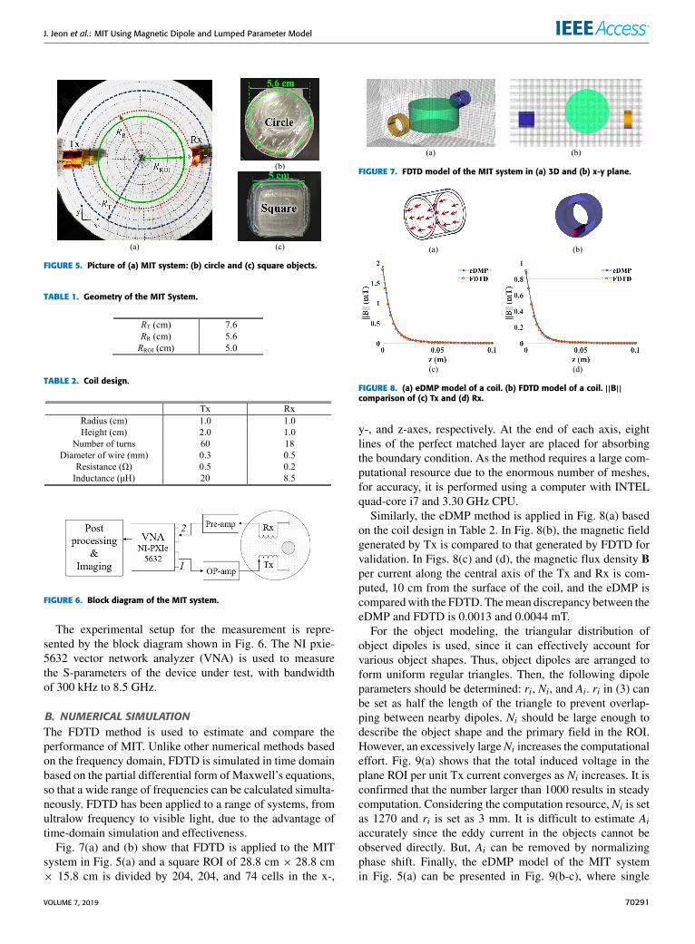
A. MIT SYSTEM SETUPThe MIT system is constructed for experiments with one setof a Tx and Rx, as shown in Fig. 5(a), and shielded fromthe external magnetic field. The geometry of the system andthe design of the Tx and Rx are detailed in Tables 1 and 2,respectively.

Physiological saline similar to the human body fluid isapplied to the object. At room temperature, the salt con-centration is 0.9 %, conductivity is 1.6 S/m, and relativepermittivity is 80. Two shapes, circle and square, are usedas the target object to examine the effect of shape. Physio-logical saline 40 ml is injected in a circle and square casein Fig. 5(b) and (c).

70290 VOLUME 7, 2019

J. Jeon et al.: MIT Using Magnetic Dipole and Lumped Parameter Model

FIGURE 5. Picture of (a) MIT system: (b) circle and (c) square objects.

TABLE 1. Geometry of the MIT System.

TABLE 2. Coil design.

FIGURE 6. Block diagram of the MIT system.

The experimental setup for the measurement is repre-sented by the block diagram shown in Fig. 6. The NI pxie-5632 vector network analyzer (VNA) is used to measurethe S-parameters of the device under test, with bandwidthof 300 kHz to 8.5 GHz.

B. NUMERICAL SIMULATIONThe FDTD method is used to estimate and compare theperformance of MIT. Unlike other numerical methods basedon the frequency domain, FDTD is simulated in time domainbased on the partial differential form of Maxwell’s equations,so that a wide range of frequencies can be calculated simulta-neously. FDTD has been applied to a range of systems, fromultralow frequency to visible light, due to the advantage oftime-domain simulation and effectiveness.

Fig. 7(a) and (b) show that FDTD is applied to the MITsystem in Fig. 5(a) and a square ROI of 28.8 cm × 28.8 cm× 15.8 cm is divided by 204, 204, and 74 cells in the x-,

FIGURE 7. FDTD model of the MIT system in (a) 3D and (b) x-y plane.

FIGURE 8. (a) eDMP model of a coil. (b) FDTD model of a coil. ||B||

comparison of (c) Tx and (d) Rx.

y-, and z-axes, respectively. At the end of each axis, eightlines of the perfect matched layer are placed for absorbingthe boundary condition. As the method requires a large com-putational resource due to the enormous number of meshes,for accuracy, it is performed using a computer with INTELquad-core i7 and 3.30 GHz CPU.

Similarly, the eDMP method is applied in Fig. 8(a) basedon the coil design in Table 2. In Fig. 8(b), the magnetic fieldgenerated by Tx is compared to that generated by FDTD forvalidation. In Figs. 8(c) and (d), the magnetic flux density Bper current along the central axis of the Tx and Rx is com-puted, 10 cm from the surface of the coil, and the eDMP iscomparedwith the FDTD. Themean discrepancy between theeDMP and FDTD is 0.0013 and 0.0044 mT.

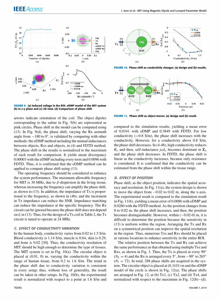
For the object modeling, the triangular distribution ofobject dipoles is used, since it can effectively account forvarious object shapes. Thus, object dipoles are arranged toform uniform regular triangles. Then, the following dipoleparameters should be determined: ri, Ni, and Ai. ri in (3) canbe set as half the length of the triangle to prevent overlap-ping between nearby dipoles. Ni should be large enough todescribe the object shape and the primary field in the ROI.However, an excessively largeNi increases the computationaleffort. Fig. 9(a) shows that the total induced voltage in theplane ROI per unit Tx current converges as Ni increases. It isconfirmed that the number larger than 1000 results in steadycomputation. Considering the computation resource, Ni is setas 1270 and ri is set as 3 mm. It is difficult to estimate Aiaccurately since the eddy current in the objects cannot beobserved directly. But, Ai can be removed by normalizingphase shift. Finally, the eDMP model of the MIT systemin Fig. 5(a) can be presented in Fig. 9(b-c), where single

VOLUME 7, 2019 70291

J. Jeon et al.: MIT Using Magnetic Dipole and Lumped Parameter Model

FIGURE 9. (a) Induced voltage in the ROI. eDMP model of the MIT system(b) in x-y plane and (c) 3D view. (d) Comparison of phase shift.

arrows indicate orientation of the coil. The object dipolescorresponding to the saline in Fig. 5(b) are represented aspink circles. Phase shift in the model can be computed using(13). In Fig. 9(d), the phase shift, varying the Rx azimuthangle from −180 to 0◦, is validated by comparing with othermethods: the eDMPmethod including themutual inductancesbetween objects, Rxs and objects, in (4) and FDTD method.The phase shift in the results is normalized to the maximumof each result for comparison. It yields mean discrepancy0.00003with the eDMP including every term and 0.0096withFDTD. Thus, it is confirmed that the eDMP method can beapplied to compute phase shift using (13).

The operating frequency should be considered to enhancethe system performance. The maximum allowable frequencyfor MIT is 30 MHz, due to β-dispersion in the living tissue,whereas increasing the frequency can amplify the phase shift,as shown in (13). In addition, the impedance of Tx is propor-tional to the frequency, as shown in (4b), and the incrementin Tx impedance can reduce the SNR. Impedance matchingcan reduce the impedance at the specific frequency. The Rxcircuit can be ignored because the phase shift does not dependon Il in (13). Thus, for the design of a Tx coil in Table 2, the Txcircuit is tuned to operate at 24 MHz.

C. EFFECT OF CONDUCTIVITY VARIATIONIn the human body, conductivity varies from 0.02 to 1.5 S/m.Blood conductivity is 1.14 S/m, muscle is 0.64, skin is 0.29,and bone is 0.02 [30]. Thus, the conductivity resolution ofMIT should be high enough to determine the type of tissues.The MIT system is set in Fig. 10(a). The circular object isplaced at (0.01, 0) m, varying the conductivity within therange of human tissue, from 0.2 to 1.6 S/m. The trend inthe phase shift due to conductivity variation is consistentin every setup; thus, without loss of generality, the resultcan be taken in other setups. In Fig. 10(b), the experimentalresult is normalized with respect to a point at 1.6 S/m and

FIGURE 10. Phase shift as conductivity changes: (a) design and (b) results.

FIGURE 11. Phase shift as object moves: (a) design and (b) result.

compared to the simulation results, yielding a mean errorof 0.0341 with eDMP and 0.3849 with FDTD. For lowconductivity (<0.8 S/m), the phase shift increases with theconductivity. However, for a conductivity above 0.8 S/m,the phase shift decreases. In (4-4b), high conductivity reducesRi, and then, self-inductance jωLi becomes dominant in Zoand the phase shift decreases. In FDTD, the phase shift islinear as the conductivity increases, because only resistanceis considered. It is confirmed that the conductivity can beestimated from the phase shift within the tissue range.

D. EFFECT OF POSITIONPhase shift, as the object position, indicates the spatial accu-racy and resolution. In Fig. 11(a), the system design is shownto move the object from −0.02 to 0.02 m, along the x-axis.The experimental result is compared to the simulation resultin Fig. 11(b), yielding a mean error of 0.0086 with eDMP and0.0260 with the FDTDmethod. As the position changes from0 to 0.02 m, the phase shift increases, and then, the positionbecomes distinguishable. However, within (−0.02-0) m, it isdifficult to determine the position because the sensitivity in(13) is uniform within the region. Arranging the Tx and Rxon a symmetrical position can improve the spatial resolutionin the region. Thus, numerous Txs and Rxs should be placedat various locations to enhance sensitivity in the entire ROI.

The relative position between the Tx and Rx can achievethe same performance as that obtained usingmultiple Txs andRxs, as shown in Fig. 3. Thus, the Tx is placed at every 90◦

(Nk = 4) and the Rx is arranged every 5◦, from−90◦ to 265◦

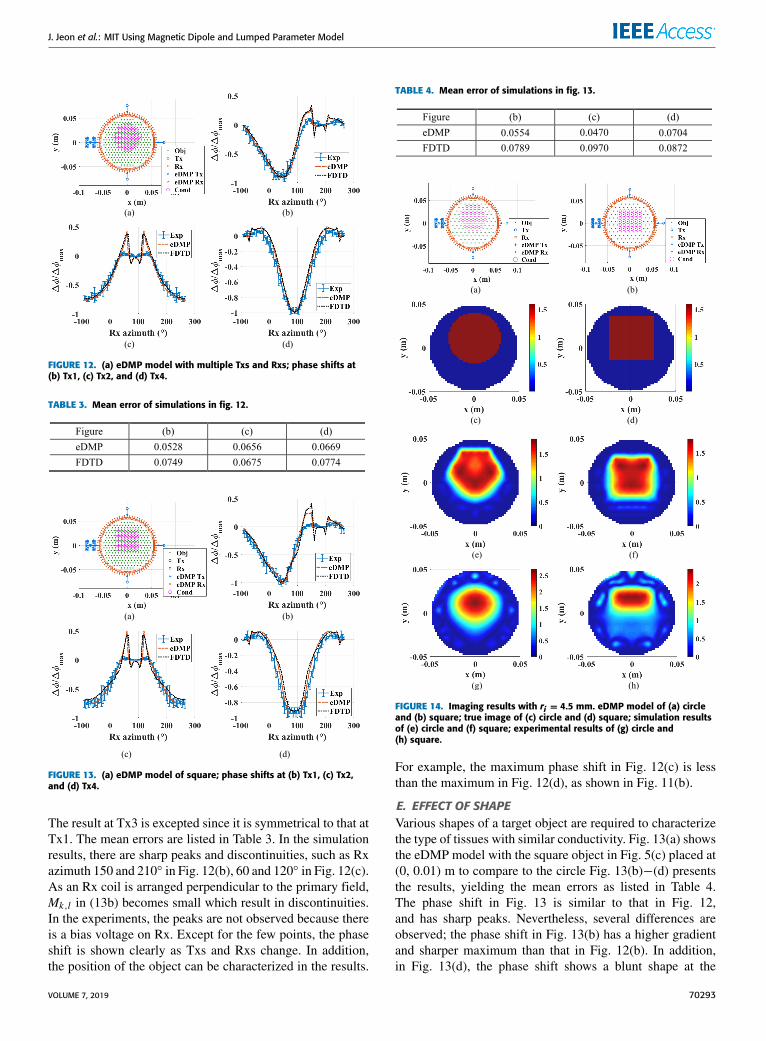
(Nl = 72). In total, 288 phase shifts are acquired in the sys-tem. The circular object is placed at (0, 0.01) m and the eDMPmodel of the circle is shown in Fig. 12(a). The phase shiftsare arranged in Fig. 12, at (b) Tx1, (c) Tx2, and (d) Tx4, andnormalized with respect to the maximum in Fig. 12(b)−(d).

70292 VOLUME 7, 2019

J. Jeon et al.: MIT Using Magnetic Dipole and Lumped Parameter Model

FIGURE 12. (a) eDMP model with multiple Txs and Rxs; phase shifts at(b) Tx1, (c) Tx2, and (d) Tx4.

TABLE 3. Mean error of simulations in fig. 12.

FIGURE 13. (a) eDMP model of square; phase shifts at (b) Tx1, (c) Tx2,and (d) Tx4.

The result at Tx3 is excepted since it is symmetrical to that atTx1. The mean errors are listed in Table 3. In the simulationresults, there are sharp peaks and discontinuities, such as Rxazimuth 150 and 210◦ in Fig. 12(b), 60 and 120◦ in Fig. 12(c).As an Rx coil is arranged perpendicular to the primary field,Mk,l in (13b) becomes small which result in discontinuities.In the experiments, the peaks are not observed because thereis a bias voltage on Rx. Except for the few points, the phaseshift is shown clearly as Txs and Rxs change. In addition,the position of the object can be characterized in the results.

TABLE 4. Mean error of simulations in fig. 13.

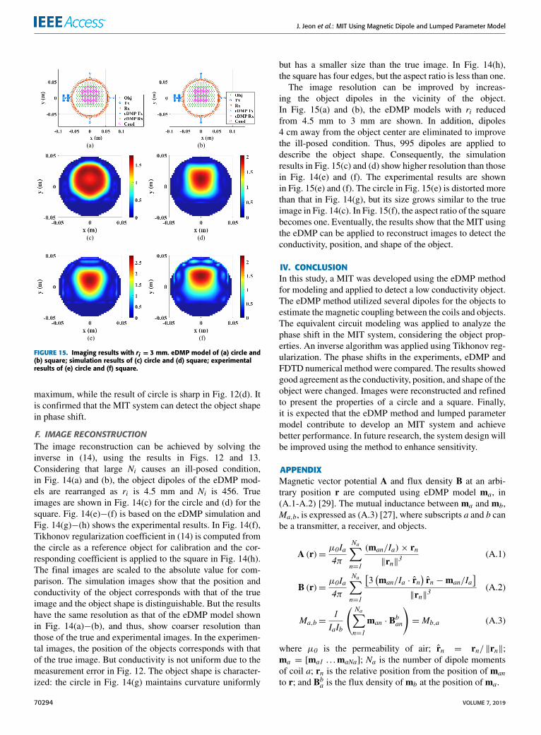
FIGURE 14. Imaging results with ri = 4.5 mm. eDMP model of (a) circleand (b) square; true image of (c) circle and (d) square; simulation resultsof (e) circle and (f) square; experimental results of (g) circle and(h) square.

For example, the maximum phase shift in Fig. 12(c) is lessthan the maximum in Fig. 12(d), as shown in Fig. 11(b).

E. EFFECT OF SHAPEVarious shapes of a target object are required to characterizethe type of tissues with similar conductivity. Fig. 13(a) showsthe eDMP model with the square object in Fig. 5(c) placed at(0, 0.01) m to compare to the circle Fig. 13(b)−(d) presentsthe results, yielding the mean errors as listed in Table 4.The phase shift in Fig. 13 is similar to that in Fig. 12,and has sharp peaks. Nevertheless, several differences areobserved; the phase shift in Fig. 13(b) has a higher gradientand sharper maximum than that in Fig. 12(b). In addition,in Fig. 13(d), the phase shift shows a blunt shape at the

VOLUME 7, 2019 70293

J. Jeon et al.: MIT Using Magnetic Dipole and Lumped Parameter Model

FIGURE 15. Imaging results with ri = 3 mm. eDMP model of (a) circle and(b) square; simulation results of (c) circle and (d) square; experimentalresults of (e) circle and (f) square.

maximum, while the result of circle is sharp in Fig. 12(d). Itis confirmed that the MIT system can detect the object shapein phase shift.

F. IMAGE RECONSTRUCTIONThe image reconstruction can be achieved by solving theinverse in (14), using the results in Figs. 12 and 13.Considering that large Ni causes an ill-posed condition,in Fig. 14(a) and (b), the object dipoles of the eDMP mod-els are rearranged as ri is 4.5 mm and Ni is 456. Trueimages are shown in Fig. 14(c) for the circle and (d) for thesquare. Fig. 14(e)−(f) is based on the eDMP simulation andFig. 14(g)−(h) shows the experimental results. In Fig. 14(f),Tikhonov regularization coefficient in (14) is computed fromthe circle as a reference object for calibration and the cor-responding coefficient is applied to the square in Fig. 14(h).The final images are scaled to the absolute value for com-parison. The simulation images show that the position andconductivity of the object corresponds with that of the trueimage and the object shape is distinguishable. But the resultshave the same resolution as that of the eDMP model shownin Fig. 14(a)−(b), and thus, show coarser resolution thanthose of the true and experimental images. In the experimen-tal images, the position of the objects corresponds with thatof the true image. But conductivity is not uniform due to themeasurement error in Fig. 12. The object shape is character-ized: the circle in Fig. 14(g) maintains curvature uniformly

but has a smaller size than the true image. In Fig. 14(h),the square has four edges, but the aspect ratio is less than one.

The image resolution can be improved by increas-ing the object dipoles in the vicinity of the object.In Fig. 15(a) and (b), the eDMP models with ri reducedfrom 4.5 mm to 3 mm are shown. In addition, dipoles4 cm away from the object center are eliminated to improvethe ill-posed condition. Thus, 995 dipoles are applied todescribe the object shape. Consequently, the simulationresults in Fig. 15(c) and (d) show higher resolution than thosein Fig. 14(e) and (f). The experimental results are shownin Fig. 15(e) and (f). The circle in Fig. 15(e) is distorted morethan that in Fig. 14(g), but its size grows similar to the trueimage in Fig. 14(c). In Fig. 15(f), the aspect ratio of the squarebecomes one. Eventually, the results show that the MIT usingthe eDMP can be applied to reconstruct images to detect theconductivity, position, and shape of the object.

IV. CONCLUSIONIn this study, a MIT was developed using the eDMP methodfor modeling and applied to detect a low conductivity object.The eDMP method utilized several dipoles for the objects toestimate the magnetic coupling between the coils and objects.The equivalent circuit modeling was applied to analyze thephase shift in the MIT system, considering the object prop-erties. An inverse algorithm was applied using Tikhonov reg-ularization. The phase shifts in the experiments, eDMP andFDTD numerical methodwere compared. The results showedgood agreement as the conductivity, position, and shape of theobject were changed. Images were reconstructed and refinedto present the properties of a circle and a square. Finally,it is expected that the eDMP method and lumped parametermodel contribute to develop an MIT system and achievebetter performance. In future research, the system design willbe improved using the method to enhance sensitivity.

APPENDIXMagnetic vector potential A and flux density B at an arbi-trary position r are computed using eDMP model ma, in(A.1-A.2) [29]. The mutual inductance between ma and mb,Ma,b, is expressed as (A.3) [27], where subscripts a and b canbe a transmitter, a receiver, and objects.

A (r)=µ0Ia4π

Na∑n=1

(man/Ia)× rn‖rn‖3

(A.1)

B (r)=µ0Ia4π

Na∑n=1

[3(man/Ia · r̂n

)r̂n −man/Ia

]‖rn‖3

(A.2)

Ma,b=1IaIb

( Na∑n=1

man · Bban

)= Mb,a (A.3)

where µ0 is the permeability of air; r̂n = rn/ ‖rn‖;ma = [ma1 . . .maNa]; Na is the number of dipole momentsof coil a; rn is the relative position from the position of manto r; and Bba is the flux density of mb at the position of ma.

70294 VOLUME 7, 2019

J. Jeon et al.: MIT Using Magnetic Dipole and Lumped Parameter Model

The magnetic flux density in (6) can be converted to vectorpotential Ai on the loop of Ii, as shown in (A.4). Ai can becomputed by substitutingmi in (A1), and hence, Li in (4b) isobtained as

Li=πr2i ‖Bi‖|Si/Ii = 2πri ‖Ai‖|ri

/Ii (A.4)

(Ai/Ii)|r=ri =µ0

4π(mi/Ii)× ri

r3i= −

µ0

4dri (A.5)

Li=µ0πri/2. (A.6)

REFERENCES[1] J. García-Martín, J. Gómez-Gil, and E. Vázquez-Sánchez,

‘‘Non-destructive techniques based on eddy current testing,’’ Sensors,vol. 11, no. 3, pp. 2525–2565, Feb. 2011.

[2] H. Griffiths, ‘‘Magnetic induction tomography,’’ Meas. Sci. Technol.,vol. 12, no. 8, pp. 1126–1131, Jun. 2001.

[3] D. Gürsoy and H. Scharfetter, ‘‘The effect of receiver coil orientations onthe imaging performance of magnetic induction tomography,’’ Meas. Sci.Technol., vol. 20, no. 10, Sep. 2009, Art. no. 105505.

[4] M. Zolgharni, H. Griffiths, and P. D. Ledger, ‘‘Frequency-difference MITimaging of cerebral haemorrhage with a hemispherical coil array: Numer-ical modelling,’’ Physiol. Meas., vol. 31, no. 8, pp. S111–S125, Jul. 2010.

[5] C. H. Igney, S.Watson, R. J.Williams, H. Griffiths, andO. Dössel, ‘‘Designand performance of a planar-array MIT system with normal sensor align-ment,’’ Physiol. Meas., vol. 26, no. 2, pp. S263–S278, Mar. 2005.

[6] C. H. Riedel, M. Keppelen, S. Nani, R. D. Merges, and O. Dössel, ‘‘Planarsystem for magnetic induction conductivity measurement using a sensormatrix,’’ Physiol. Meas., vol. 25, no. 1, pp. 403–411, Feb. 2004.

[7] B. U. Karbeyaz and N. G. Gencer, ‘‘Electrical conductivity imaging viacontactless measurements: An experimental study,’’ IEEE Trans. Med.Imag., vol. 22, no. 5, pp. 627–635, May 2003.

[8] S. Hermann, K. L. Helmut, and R. Javier, ‘‘Magnetic induction tomogra-phy: Hardware for multi-frequency measurements in biological tissues,’’Physiol. Meas., vol. 22, no. 1, pp. 131–146, 2001.

[9] D. Gürsoy and H. Scharfetter, ‘‘Imaging artifacts in magnetic inductiontomography caused by the structural incorrectness of the sensor model,’’Meas. Sci. Technol., vol. 22, no. 1, Dec. 2011, Art. no. 015502.

[10] C. Deans, L. Marmugi, S. Hussain, and F. Renzoni, ‘‘Electromagneticinduction imaging with a radio-frequency atomic magnetometer,’’ Appl.Phys. Lett., vol. 108, no. 10, Mar. 2016, Art. no. 103503.

[11] K. Stawicki, S. Gratkowski, M. Komorowski, and T. Pietrusewicz,‘‘A new transducer for magnetic induction tomography,’’ IEEE Trans.Magn., vol. 45, no. 3, pp. 1832–1835, Mar. 2009.

[12] C. Tan, Y. Wu, Z. Xiao, and F. Dong, ‘‘Optimization of dualfrequency-difference MIT sensor array based on sensitivity and resolutionanalysis,’’ IEEE Access, vol. 6, pp. 34911–34920, 2018.

[13] H.-Y.Wei andM. Soleimani, ‘‘Hardware and software design for a nationalinstrument-based magnetic induction tomography system for prospectivebiomedical applications,’’ Physiol. Meas., vol. 33, no. 5, pp. 863–879,Apr. 2012.

[14] J. R. Feldkamp, ‘‘Single-coil magnetic induction tomographic three-dimensional imaging,’’ J. Med. Imag., vol. 2, no. 1, Mar. 2015,Art. no. 013502.

[15] C. A. González, C. Villanueva, C. Vera, O. Flores, R. D. Reyes, andB. Rubinsky, ‘‘The detection of brain ischaemia in rats by inductive phaseshift spectroscopy,’’ Physiol. Meas., vol. 30, pp. 809–819, Jun. 2009.

[16] G. Jin, J. Sun, M. Qin, Q. Tang, L. Xu, X. Ning, J. Xu, X. Pu, andM. Chen,‘‘A new method for detecting cerebral hemorrhage in rabbits by magneticinductive phase shift,’’Biosensors Bioelectron., vol. 52, no. 4, pp. 374–378,2014.

[17] S. Zhao, G. Li, S. Gu, J. Ren, J. Chen, L. Xu, M. Chen, J. Yang,K. W. Leung, and J. Sun, ‘‘An experimental study of relationship betweenmagnetic induction phase shift and brain parenchyma volume with brainedema in traumatic brain injury,’’ IEEE Access, vol. 7, pp. 20974–20983,Feb. 2019.

[18] M. Soleimani, W. R. B. Lionheart, and A. J. Peyton, ‘‘Image reconstructionfor high-contrast conductivity imaging in mutual induction tomographyfor industrial applications,’’ IEEE Trans. Instrum. Meas., vol. 56, no. 5,pp. 2024–2032, Oct. 2007.

[19] L. Ma, S. Spagnul, and M. Soleimani, ‘‘Metal solidification imagingprocess by magnetic induction tomography,’’ Sci. Rep., vol. 7, no. 1,Nov. 2017, Art. no. 14502.

[20] Y. Zhou, Q.Ma, G. Guo, J. Tu, and D. Zhang, ‘‘Magneto-acousto-electricalmeasurement based electrical conductivity reconstruction for tissues,’’IEEE Trans. Biomed. Eng., vol. 65, no. 5, pp. 1086–1094, May 2018.

[21] L. Wang and A. M. Al-Jumaily, ‘‘Imaging of lung structure usingholographic electromagnetic induction,’’ IEEE Access, vol. 5,pp. 20313–20318, 2017.

[22] R. Merwa, K. Hollaus, B. Brandstätter, and H. Scharfetter, ‘‘Numericalsolution of the general 3D eddy current problem for magnetic inductiontomography (spectroscopy),’’ Physiol. Meas., vol. 24, no. 2, pp. 545–554,Apr. 2003.

[23] L. Ma and M. Soleimani, ‘‘Magnetic induction tomography methods andapplications: A review,’’ Meas. Sci. Technol., vol. 28, no. 7, Jun. 2017,Art. no. 072001.

[24] Q. Wang, Practical Design of Magnetostatic Structure Using NumericalSimulation. Hoboken, NJ, USA: Wiley, 2013.

[25] N. DeGeeter, G. Crevecoeur, and L. Dupré, ‘‘An efficient 3-D eddy-currentsolver using an independent impedance method for transcranial magneticstimulation,’’ IEEE Trans. Biomed. Eng., vol. 58, no. 2, pp. 310–320,Feb. 2011.

[26] Z. Xiao, C. Tan, and F. Dong, ‘‘Effect of inter-tissue inductive cou-pling on multi-frequency imaging of intracranial hemorrhage by magneticinduction tomography,’’ Meas. Sci. Technol., vol. 28, no. 8, Jul. 2017,Art. no. 084001.

[27] F. Wu, J. Jeon, S. K. Moon, H. J. Choi, and H. Son, ‘‘Voice coil navigationsensor for flexible silicone intubation,’’ IEEE/ASME Trans. Mechatronics,vol. 21, no. 2, pp. 851–859, Apr. 2016.

[28] F. Wu, S. K. Moon, and H. Son, ‘‘Orientation measurement based on mag-netic inductance by the extended distributed multi-pole model,’’ Sensors,vol. 14, pp. 11504–11521, Jun. 2014.

[29] J. Jeon and H. Son, ‘‘Active control of magnetic field using eDMP modelfor biomedical applications,’’ IEEE/ASME Trans. Mechatronics, vol. 23,no. 1, pp. 29–37, Feb. 2018.

[30] P. A. Hasgall. (May 15, 2018). IT’IS Database for Thermal and Electro-magnetic Parameters of Biological Tissues. [Online]. Available: http://itis.swiss/database

JIYUN JEON received the B.S. degree in mechan-ical and nuclear engineering from the UlsanNational Institute of Science and Technology(UNIST), Ulsan, South Korea, in 2014, whereshe is currently pursuing the Ph.D. degree withthe School of Mechanical, Aerospace and NuclearEngineering. Her research interests include mag-netic sensors, magnetic induction tomography, andmagnetic field design.

WONMO CHUNG received the B.S. degree inmechanical and nuclear engineering from theUlsan National Institute of Science and Technol-ogy (UNIST), Ulsan, South Korea, in 2016, wherehe is currently pursuing the Ph.D. degree withthe School of Mechanical, Aerospace and NuclearEngineering. His research interests include mag-netic sensors, magnetic induction tomography, androbust control of UAV.

HUNGSUN SON (S’07–M’09) received the M.S.degree in aero and astronautical engineering fromStanford University, Stanford, CA, USA, in 2002,and the Ph.D. degree in mechanical engineeringfrom the Georgia Institute of Technology, Atlanta,in 2007. He is currently an Associate Professorin mechanical, aerospace, and nuclear engineeringwith the Ulsan National Institute of Science andTechnology (UNIST), South Korea. His currentresearch interests include mechatronics, sensors

and actuators, dynamic system modeling, design optimization, automation,and control.

VOLUME 7, 2019 70295