Magnetic induction tomography guided

electrical capacitance tomography imaging with

grounded conductors

Maomao Zhang, Lu Ma, Manuchehr Soleimani

Egnineering Tomography Laborotory (ETL), Department of Electronic and Electrical Engineering,

University of Bath, Bath, UK

Abstract –Electrical capacitance tomography (ECT) is an imaging technique

commonly used for imaging dielectric permittivity of insulating objects. In applications

such industrial process tomography and non-destructive testing (NDT), the objects under test

may exhibit variations in both dielectric permittivity and electrical conductivity. In particular,

a sample that includes high conductivity, such as metal, can cause a large change in electrical

field in ECT. The metal sample in imaging area will cause a large change in the sensitivity

map of ECT compared to free space, which will make the ECT image reconstruction

inaccurate. This effect is more severe in grounded conductor than floating conductors, so this

paper focuses on grounded conductor. In order to update the sensitivity map, one needs to

gain information about the conductivity distribution in ECT problem. Magnetic induction

tomography (MIT) is sensitive to electrical conductivity and not sensitive to permittivity

variations; therefore, it can be used to visualize the conductivity distribution of the target

under test. In this paper, a dual-modality MIT and ECT system is proposed to image a

medium including conductors and dielectrics. Both simulated and experimental results are

presented, which demonstrate the feasibility of the proposed method.

Keywords: Dual- modality ECT/MIT, dielectric imaging with grounded conductors,

sensitivity map.

1. Introduction

Electrical capacitance tomography (ECT) is a non-invasive technology that can be used to

monitor industrial processes or defect detections in non-destructive testing (NDT). The aim of

ECT is to visualize the unknown permittivity distribution via measuring capacitances between

pairs of peripheral electrodes around the samples. Recent applications of ECT include

monitoring gas-solid flows in pneumatic conveyors and gas-oil in oil pipeline [1, 2].

Typically, a time difference imaging is used in ECT image reconstruction. The change in

permittivity is reconstructed by the sensitivity map of reference condition and the difference

between reference measurements and sample measurements [3]. Therefore, the accuracy of a

sensitivity map has a significant effect on results of ECT image reconstruction.

When there are grounded conductors in ECT sensor area, the electric fields will be

significantly different than that of a medium with only dielectric materials. Therefore, the

sensitivity map of a typical reference condition, i.e. air-filled sensor, is not accurate [4]. To

decrease the effect of increased nonlinearity caused by high conductivity, a precise forward

model must be introduced. This modified model, which is close to the real physical scenario,

includes the highly conductive content, which is modelled as grounded conductor. The

previous study of metal in an ECT sensor has been done by Ville Rimpiläinena et al. [5],

where the high-shear mixer has a typical structure with a metal shaft in the centre. For better

quality of visualization of the process in the mixer, the known position and size of central

shaft was taken into account. Similar to the method used in EIT with metallic samples in [6],

the surface of metal is regarded as one electrode of the sensor, and it is considered

electrically grounded. Furthermore, the boundary condition on conductor is set at zero voltage.

In all above applications location of grounded conductors are known. Here we extended this

to the case that the location of conductor is unknown.

To detect and identify the high conductivity in ECT imaging, magnetic induction tomography

(MIT) imaging is used. Using the location of grounded metal a precise sensitivity map in

ECT is created. MIT aims to visualized the distribution of passive electromagnetic properties

in particular permeability 𝜇 or conductivity 𝜎 [7]. In MIT, the magnetic field induces eddy

currents in the conductive object, which produces a change in the magnetic field received by

the receiver coils. This paper proposes a combined MIT and ECT system as a dual modality

imaging solution for imaging metallic and dielectric samples. MIT is not sensitive to

dielectric permittivity variations, which allows a sequential data fusion to be adapted on this

dual modality method. The information of electrical conductivity from MIT feeds into the

ECT image reconstruction software allowing reconstruction of both conductivity and

permittivity. Compared to the dual-modality electrical resistance tomography systems (ERT)

and ECT [8, 9], ECT and MIT combination offers a fully contactless imaging solution. ERT

requires electrical connection to objects making it unsuitable for many applications. In [10], a

two electrode capacitive measurement system is used to image either void (dielectric

permittivity change) or rebar (metal) . In this paper we propose a dual modality method, in

which dielectric permittivity changes and grounded conductor can be monitored

simultaneously. This dual modality imaging method provides a wider range of applications

for ECT, where the conductive media between an object and a sensor is not known. This

paper demonstrates that the ECT imaging capability of dielectric variations will be

substantially reduced, in particular when the ground conductors are close to the dielectric

inclusions. The dual modality has potential applications for mixture of both conductive and

dielectric samples, such as defect detection for steel reinforced concrete.

The aim of this paper is to investigate a dual modality imaging for a combination of ground

conductors and dielectric inclusions using MIT and ECT. The structure of the paper is

organised as follows. In section 2, the ECT and MIT hardware and models are introduced. In

section 3, the error tolerance of ECT is will be evaluated by the figure of merits, which is

developed by Andy Adler et al.[11]. In section Error! Reference source not found., the

experiment of dual-modality MIT/ECT is conducted, and the final results are assessed.

2. ECT and MIT hardware and models

Here we briefly describe ECT and MIT system, sensor and forward modelling and sensitivity

maps. A 16 channel MIT system and a 12 channel ECT system is used for sequential data

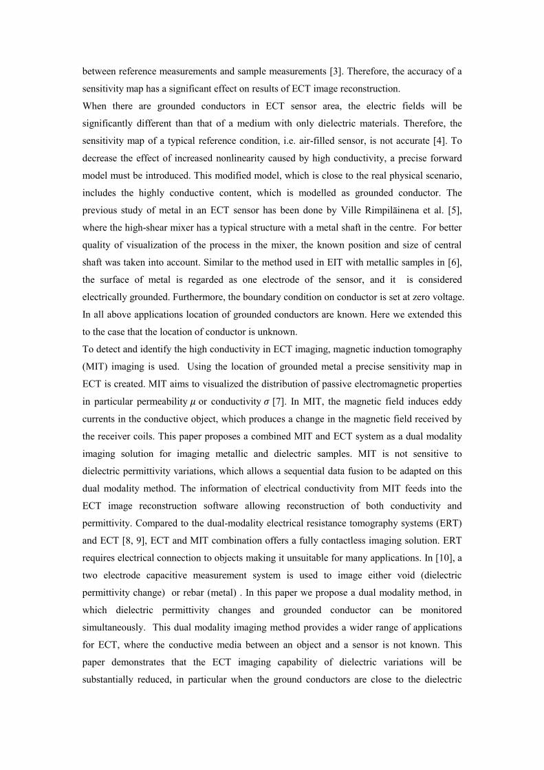
fusion in dual modality ECT and MIT imaging, Figure 1 shows both sensor arrays.

(a) (b)

Figure 1. (a) The 12-electrode ECT sensor; (b) The 16-coil MIT sensor.

2.1 ECT

A typical ECT sensor consists of 6, 8, 12 or 24 electrodes [12], which are evenly mounted

outside a pipe-shaped non-conductive wall and separated with radial screens. And an external

screen for shielding the noise from outside is installed. All electrically grounded screens

reduce the effect of the external capacitance between pairs of electrodes. In some special

cases, where the wall is conductive, the electrodes are built on the inner surface of the wall,

like a metal vessel or pipe.

Figure 1(a) is the ECT sensor used in our experiment, which is composed of a plastic pipe,

12 electrodes, radial screen between the electrodes and external shielding. The external

diameter of pipe is 150 mm, the size of the electrode is 217×32 mm2 and the screens between

the electrodes are 3 mm wide. The capacitance measurement unit is the PTL 300E ECT

system, whose excitation frequency is fixed at 1.25MHz. Twelve channels are connected to

the electrodes to measure the inter-capacitance.

Forward problem of ECT is to calculate the capacitance, 𝐶, for give values of the known

permittivity distribution, 𝜀(𝑥, 𝑦), over a given geometric region and excitation signal (the

voltage of the excited electrode, 𝑢). During the measurement, one electrode is selected for

excitation and the other electrodes are grounded as detectors, then this protocol will be

applied to each electrode in turn. Maxwell’s equations in electro quasi-static are applied to

solve the forward problem of ECT [13]. The propagation effects can be neglected, since the

dimensions of the sensor are much smaller than the wavelength of the signal wave in low

frequency (10Hz-2MHz). The ECT governing equation is

∇ ∙ 𝜀(𝑥, 𝑦)∇𝑢(𝑥, 𝑦) = 0 in Ω (1)

where 𝑢(𝑥, 𝑦) is the electric potential. And the potential on the excited electrodes is known as

𝑢(𝑥, 𝑦) = V on 𝑆𝑖 (2)

And potential on sensing electrodes are

𝑢(𝑥, 𝑦) = 0 on 𝑆𝑗 (3)

where 𝑆𝑖 and 𝑆𝑗 are the surface of the excited and receiver electrodes respectively, and V is

the excitation voltage.

The derivative form of electrical potential is applied in the equation of electric charge, 𝑄𝑗, on

the excited electrode, 𝑆𝑗:

𝑄𝑗 = − ∫ 𝜀(𝑥, 𝑦)𝜕𝑢(𝑥,𝑦)

𝜕𝒏𝑒𝑗𝑑𝑆 (4)

where 𝒏 is the inward normal of 𝑆𝑙.

Therefore the capacitance between electrodes i and j can be expressed as a function of

permittivity distribution.

𝐶𝑖𝑗 =𝑄𝑗

𝑉= 𝑓(𝜀(𝑥, 𝑦)) (5)

Based on finite element method (FEM), the permittivity distribution is divided into 𝑛

elements. And the forward problem can be solved to calculate the potential distribution,

distribution of electric fields and estimated capacitance measurements.

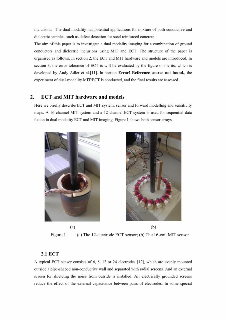
The sensitivity map can be calculated using an efficient formulation based on calculated

fields from excitation and sensing electrodes [4].

𝜕𝐶𝑖𝑗

𝜕ℰ= − ∫ ∇𝑢𝑖∇𝑢𝑗𝑑𝑆

Ω (6)

where 𝑢𝑖 and 𝑢𝑗 are potential over region Ω when electrodes 𝑖 and electrode 𝑗 are excitation

electrodes respectively.

Then the perturbation of the permittivity distribution brings the change in the electric charge

on electrode 𝑙 has been given in [4] and [14].

∆𝐶 = [𝜕𝐶1(𝜀)

𝜕𝜀1

𝜕𝐶2(𝜀)

𝜕𝜀2⋯

𝜕𝐶𝑙(𝜀)

𝜕𝜀𝑛]

1∗𝑛∗ [

∆𝜀1

∆𝜀2

⋮∆𝜀𝑛

]

𝑛∗1

(7)

In the case of free space, the sensitivity map of a pair of electrodes is shown in Figure 2. The

shallow valley indicates sensitivity distribution of a measurement between a pair of electrodes

in opposite position.

Figure 2. The sensitivity of opposite capacitance measurement in free space

2.2 MIT

A 16 channel low frequency (50 kHz excitation for metallic imaging) MIT system is used to

realise the proposed dual-modality imaging technique. The MIT system consists of: (1) a coil

array of sixteen air-cored inductive sensors, shown in Figure 1(b); (2) a sixteen channel

multiplexer for channel switching; (3) a national instrument (NI-6295) data acquisition card;

and (4) a host computer, where the data process and image reconstruction take place. This

system was designed to measure targeted object(s) with high conductivity, which corresponds

to a negative imaginary part of the magnetic field perturbation, as such, the measurements can

be approximated by their amplitudes, the phase shifts are therefore neglected [15]. The

system development has been reported in[16], and many applications have been proposed

using this system architecture.

To solve the forward problem, finding the magnetic vector potential 𝐴 is the key. There are

many FEM based formulations can be used to solve the A field, such as (A,A-V) and (A,A)

formulation. In this study, we adopted a (A, A) formulation using edge based FEM [17, 18].

∇ × ((1

𝜇) ∇ × 𝐴) + 𝑗𝜔𝜎𝐴 = 𝐽𝑠 (8)

where 𝜎 is conductivity, 𝜔 is angular frequency of the excitation current, 𝜇 is permeability,

and current density 𝐽𝑠 can be prescribed by magnetic vector potential from the Biot-Savart

Law. If the total current in the excitation coil was 𝐼0 the sensitivity of the induced voltage to

the conductivity change can be written as:

𝜕𝑉𝑚𝑛

𝜕𝜎𝑘= −𝜔2

∫ 𝐴𝑚𝐴𝑛𝑑𝑣Ω𝑘

𝐼0 (9)

where 𝑉𝑚𝑛 is the measured voltage, 𝜎𝑘 is the conductivity of pixel 𝑘, Ω𝑘 is the volume of the

perturbation (pixel 𝑘), 𝐴𝑚 and 𝐴𝑛 are respectively solutions of the forward problem when

excitation coil (𝑚) is excited by 𝐼0 and sensing coil (𝑛) is excited with unit current.

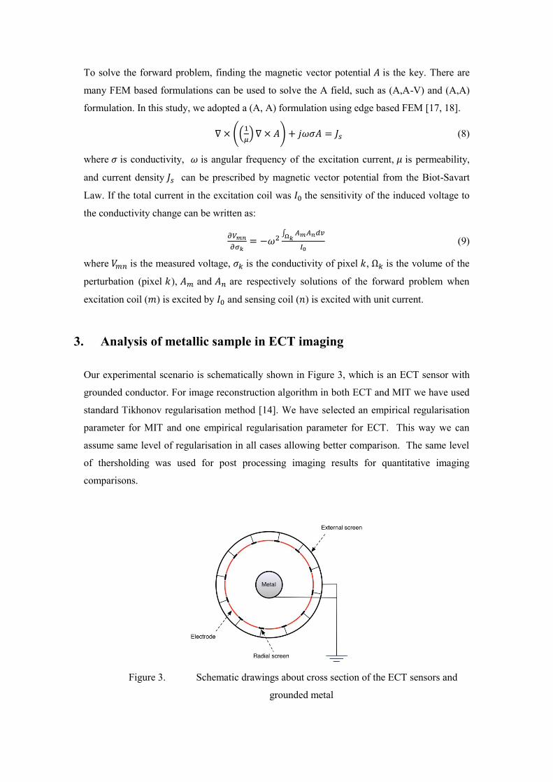
3. Analysis of metallic sample in ECT imaging

Our experimental scenario is schematically shown in Figure 3, which is an ECT sensor with

grounded conductor. For image reconstruction algorithm in both ECT and MIT we have used

standard Tikhonov regularisation method [14]. We have selected an empirical regularisation

parameter for MIT and one empirical regularisation parameter for ECT. This way we can

assume same level of regularisation in all cases allowing better comparison. The same level

of thersholding was used for post processing imaging results for quantitative imaging

comparisons.

Figure 3. Schematic drawings about cross section of the ECT sensors and

grounded metal

3.1 Reference measurement: In our experiment the sample under test consists of a metallic bar and a wooden bar.

Traditional ECT utilizes the difference between the reference capacitance (Cr) and the

measured capacitance of the sample (Cm) to visualize the dielectric distribution change. In the

case of sensing a mixture of a metallic sample and a dielectric sample, without knowing the

existence of the metal, the capacitance measurement of the air-fulfilled sensor (Cair), is chosen

as the background data (or reference data). The difference between the measurement of

samples (Cm) and Cair is utilized to solve the inverse problems; however the metal will affect

the imaging on the rest of dielectric region. Therefore choosing the capacitance measurement

of metal and air, (Cmetal+air) as the reference measurement describes the real condition more

precisely.

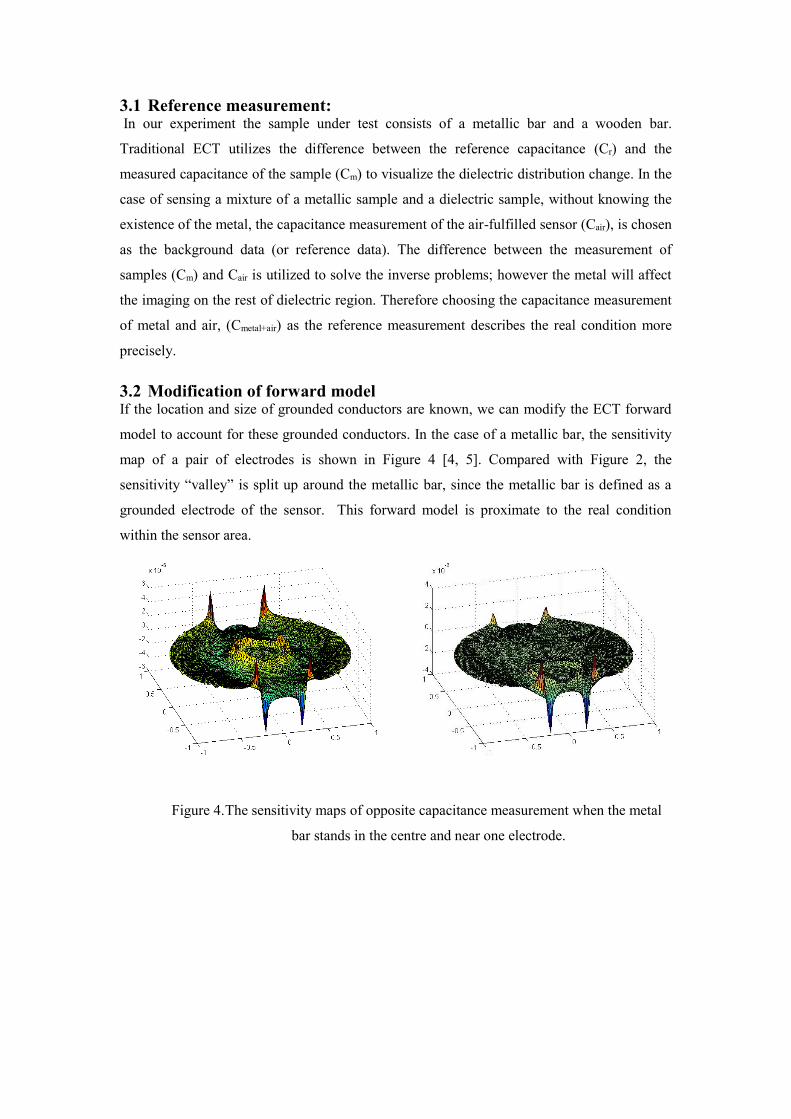
3.2 Modification of forward model If the location and size of grounded conductors are known, we can modify the ECT forward

model to account for these grounded conductors. In the case of a metallic bar, the sensitivity

map of a pair of electrodes is shown in Figure 4 [4, 5]. Compared with Figure 2, the

sensitivity “valley” is split up around the metallic bar, since the metallic bar is defined as a

grounded electrode of the sensor. This forward model is proximate to the real condition

within the sensor area.

Figure 4. The sensitivity maps of opposite capacitance measurement when the metal

bar stands in the centre and near one electrode.

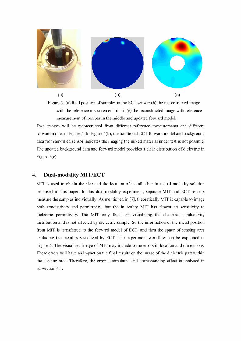
(a) (b) (c)

Figure 5. (a) Real position of samples in the ECT sensor; (b) the reconstructed image

with the reference measurement of air; (c) the reconstructed image with reference

measurement of iron bar in the middle and updated forward model.

Two images will be reconstructed from different reference measurements and different

forward model in Figure 5. In Figure 5(b), the traditional ECT forward model and background

data from air-filled sensor indicates the imaging the mixed material under test is not possible.

The updated background data and forward model provides a clear distribution of dielectric in

Figure 5(c).

4. Dual-modality MIT/ECT

MIT is used to obtain the size and the location of metallic bar in a dual modality solution

proposed in this paper. In this dual-modality experiment, separate MIT and ECT sensors

measure the samples individually. As mentioned in [7], theoretically MIT is capable to image

both conductivity and permittivity, but the in reality MIT has almost no sensitivity to

dielectric permittivity. The MIT only focus on visualizing the electrical conductivity

distribution and is not affected by dielectric sample. So the information of the metal position

from MIT is transferred to the forward model of ECT, and then the space of sensing area

excluding the metal is visualized by ECT. The experiment workflow can be explained in

Figure 6. The visualized image of MIT may include some errors in location and dimensions.

These errors will have an impact on the final results on the image of the dielectric part within

the sensing area. Therefore, the error is simulated and corresponding effect is analysed in

subsection 4.1.

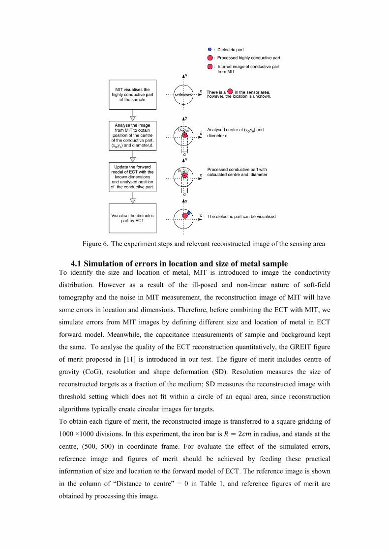
Figure 6. The experiment steps and relevant reconstructed image of the sensing area

4.1 Simulation of errors in location and size of metal sample To identify the size and location of metal, MIT is introduced to image the conductivity

distribution. However as a result of the ill-posed and non-linear nature of soft-field

tomography and the noise in MIT measurement, the reconstruction image of MIT will have

some errors in location and dimensions. Therefore, before combining the ECT with MIT, we

simulate errors from MIT images by defining different size and location of metal in ECT

forward model. Meanwhile, the capacitance measurements of sample and background kept

the same. To analyse the quality of the ECT reconstruction quantitatively, the GREIT figure

of merit proposed in [11] is introduced in our test. The figure of merit includes centre of

gravity (CoG), resolution and shape deformation (SD). Resolution measures the size of

reconstructed targets as a fraction of the medium; SD measures the reconstructed image with

threshold setting which does not fit within a circle of an equal area, since reconstruction

algorithms typically create circular images for targets.

To obtain each figure of merit, the reconstructed image is transferred to a square gridding of

1000 ×1000 divisions. In this experiment, the iron bar is 𝑅 = 2𝑐𝑚 in radius, and stands at the

centre, (500, 500) in coordinate frame. For evaluate the effect of the simulated errors,

reference image and figures of merit should be achieved by feeding these practical

information of size and location to the forward model of ECT. The reference image is shown

in the column of “Distance to centre” = 0 in Table 1, and reference figures of merit are

obtained by processing this image.

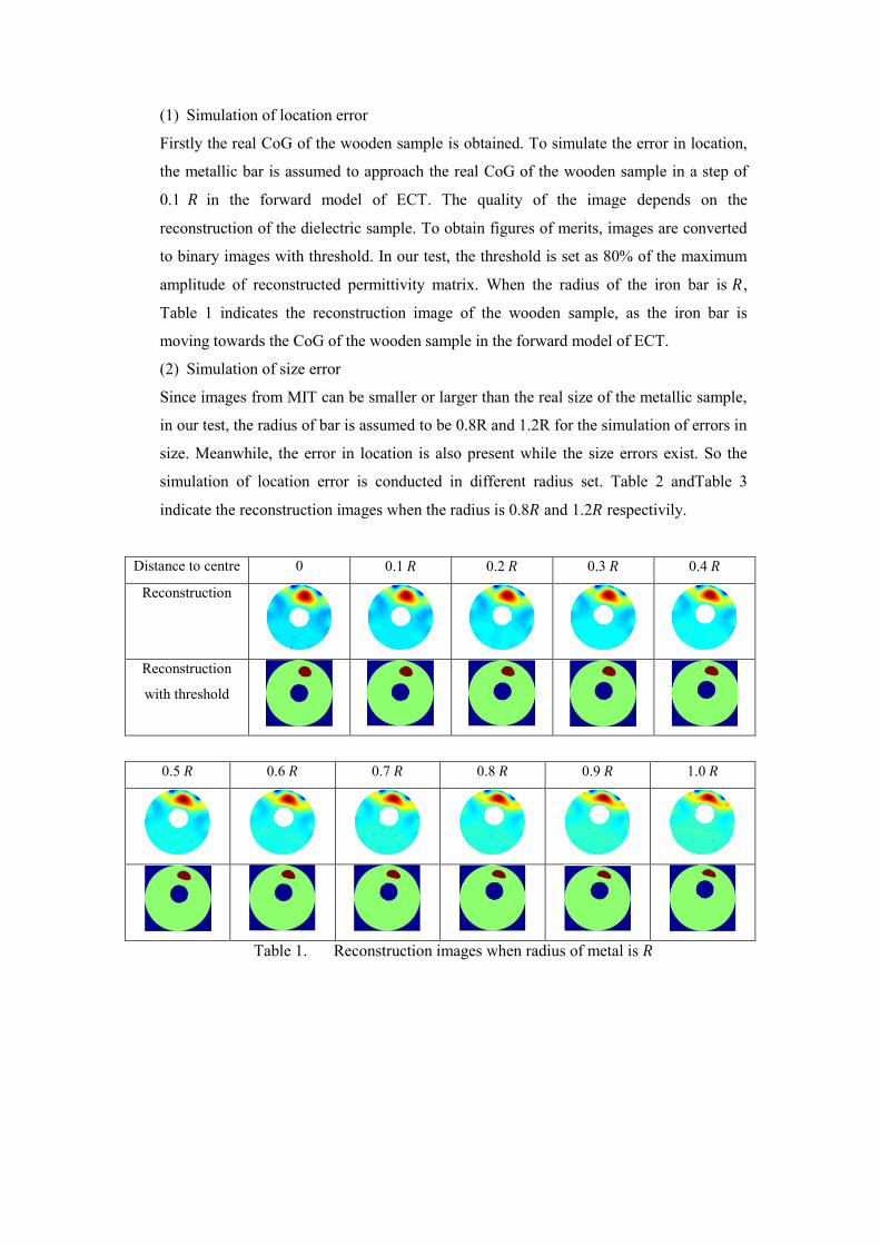
(1) Simulation of location error

Firstly the real CoG of the wooden sample is obtained. To simulate the error in location,

the metallic bar is assumed to approach the real CoG of the wooden sample in a step of

0.1 𝑅 in the forward model of ECT. The quality of the image depends on the

reconstruction of the dielectric sample. To obtain figures of merits, images are converted

to binary images with threshold. In our test, the threshold is set as 80% of the maximum

amplitude of reconstructed permittivity matrix. When the radius of the iron bar is 𝑅,

Table 1 indicates the reconstruction image of the wooden sample, as the iron bar is

moving towards the CoG of the wooden sample in the forward model of ECT.

(2) Simulation of size error

Since images from MIT can be smaller or larger than the real size of the metallic sample,

in our test, the radius of bar is assumed to be 0.8R and 1.2R for the simulation of errors in

size. Meanwhile, the error in location is also present while the size errors exist. So the

simulation of location error is conducted in different radius set. Table 2 andTable 3

indicate the reconstruction images when the radius is 0.8𝑅 and 1.2𝑅 respectivily.

Distance to centre 0 0.1 𝑅 0.2 𝑅 0.3 𝑅 0.4 𝑅

Reconstruction

Reconstruction

with threshold

0.5 𝑅 0.6 𝑅 0.7 𝑅 0.8 𝑅 0.9 𝑅 1.0 𝑅

Table 1. Reconstruction images when radius of metal is 𝑅

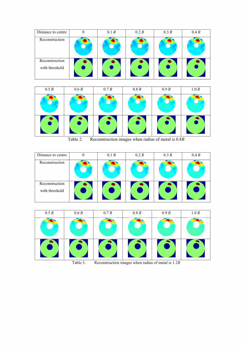
Distance to centre 0 0.1 𝑅 0.2 𝑅 0.3 𝑅 0.4 𝑅

Reconstruction

Reconstruction

with threshold

0.5 𝑅 0.6 𝑅 0.7 𝑅 0.8 𝑅 0.9 𝑅 1.0 𝑅

Table 2. Reconstruction images when radius of metal is 0.8𝑅

Distance to centre 0 0.1 𝑅 0.2 𝑅 0.3 𝑅 0.4 𝑅

Reconstruction

Reconstruction

with threshold

0.5 𝑅 0.6 𝑅 0.7 𝑅 0.8 𝑅 0.9 𝑅 1.0 𝑅

Table 3. Reconstruction images when radius of metal is 1.2𝑅

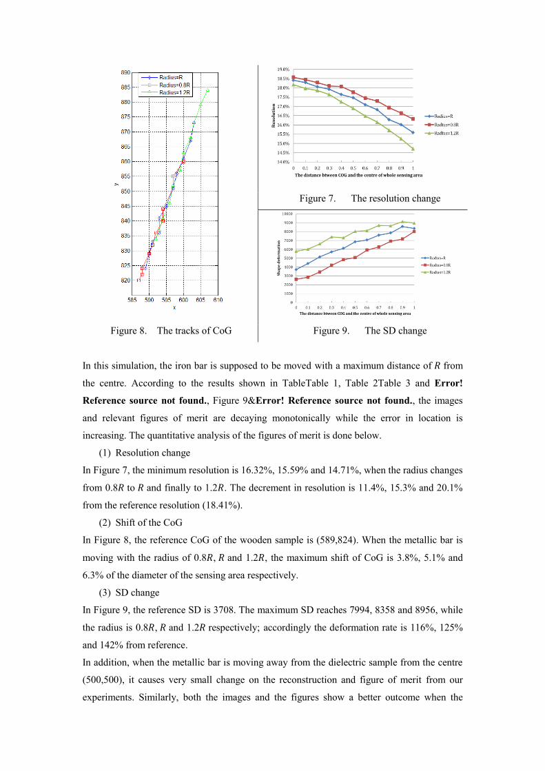
Figure 7. The resolution change

Figure 8. The tracks of CoG Figure 9. The SD change

In this simulation, the iron bar is supposed to be moved with a maximum distance of 𝑅 from

the centre. According to the results shown in TableTable 1, Table 2Table 3 and Error!

Reference source not found., Figure 9&Error! Reference source not found., the images

and relevant figures of merit are decaying monotonically while the error in location is

increasing. The quantitative analysis of the figures of merit is done below.

(1) Resolution change

In Figure 7, the minimum resolution is 16.32%, 15.59% and 14.71%, when the radius changes

from 0.8𝑅 to 𝑅 and finally to 1.2𝑅. The decrement in resolution is 11.4%, 15.3% and 20.1%

from the reference resolution (18.41%).

(2) Shift of the CoG

In Figure 8, the reference CoG of the wooden sample is (589,824). When the metallic bar is

moving with the radius of 0.8𝑅, 𝑅 and 1.2𝑅, the maximum shift of CoG is 3.8%, 5.1% and

6.3% of the diameter of the sensing area respectively.

(3) SD change

In Figure 9, the reference SD is 3708. The maximum SD reaches 7994, 8358 and 8956, while

the radius is 0.8𝑅, 𝑅 and 1.2𝑅 respectively; accordingly the deformation rate is 116%, 125%

and 142% from reference.

In addition, when the metallic bar is moving away from the dielectric sample from the centre

(500,500), it causes very small change on the reconstruction and figure of merit from our

experiments. Similarly, both the images and the figures show a better outcome when the

radius is 0.8𝑅, where reduction in size results in the same effect caused by movement of the

iron bar away from the wooden sample.

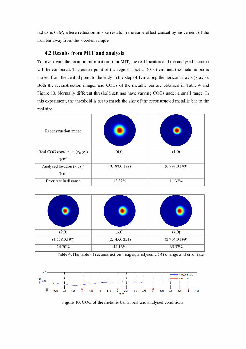
4.2 Results from MIT and analysis

To investigate the location information from MIT, the real location and the analysed location

will be compared. The centre point of the region is set as (0, 0) cm, and the metallic bar is

moved from the central point to the eddy in the step of 1cm along the horizontal axis (x-axis).

Both the reconstruction images and COGs of the metallic bar are obtained in Table 4 and

Figure 10. Normally different threshold settings have varying COGs under a small range. In

this experiment, the threshold is set to match the size of the reconstructed metallic bar to the

real size.

Reconstruction image

Real COG coordinate (𝑥0, 𝑦0)

/(cm)

(0,0) (1,0)

Analysed location (𝑥𝑖 , 𝑦𝑖)

/(cm)

(0.188,0.188) (0.797,0.100)

Error rate in distance 13.32% 11.32%

(2,0) (3,0) (4,0)

(1.558,0.197) (2.145,0.221) (2.704,0.199)

24.20% 44.16% 65.57%

Table 4. The table of reconstruction images, analysed COG change and error rate

Figure 10. COG of the metallic bar in real and analysed conditions

In Table 4 both the practical and analysed location of COG are listed. The location error rate

is defined as the equation below:

location error rate (LER) =‖(𝑥𝑖,𝑦𝑖)−(𝑥0,𝑦0)‖

𝑅 (9)

In section 3, the simulation is conducted under the condition that the metallic bar is shifted

from 0.1 𝑅 to 1 𝑅 in forward model of ECT, so the coefficient before 𝑅 represents the

simulated LER. In Figure 10, in comparison to the real COG, the COG from MIT is pulled

back to centre along x-axis. If the metallic bar is placed further from centre, the LER is

increasingly larger. Due to the symmetric structure of MIT sensor, the shifts happened in y-

axis is caused by the inevitable inaccuracy in placing the metallic bar along the x-axis during

experiments. These analysed data of COG are inputted to the forward model of ECT.

Subsequently the reconstruction images and the figures of merits will judge the quality of

dual-modality.

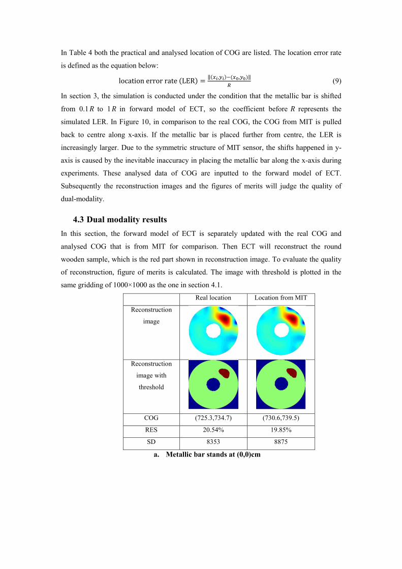
4.3 Dual modality results

In this section, the forward model of ECT is separately updated with the real COG and

analysed COG that is from MIT for comparison. Then ECT will reconstruct the round

wooden sample, which is the red part shown in reconstruction image. To evaluate the quality

of reconstruction, figure of merits is calculated. The image with threshold is plotted in the

same gridding of 1000×1000 as the one in section 4.1.

Real location Location from MIT

Reconstruction

image

Reconstruction

image with

threshold

COG (725.3,734.7) (730.6,739.5)

RES 20.54% 19.85%

SD 8353 8875

a. Metallic bar stands at (0,0)cm

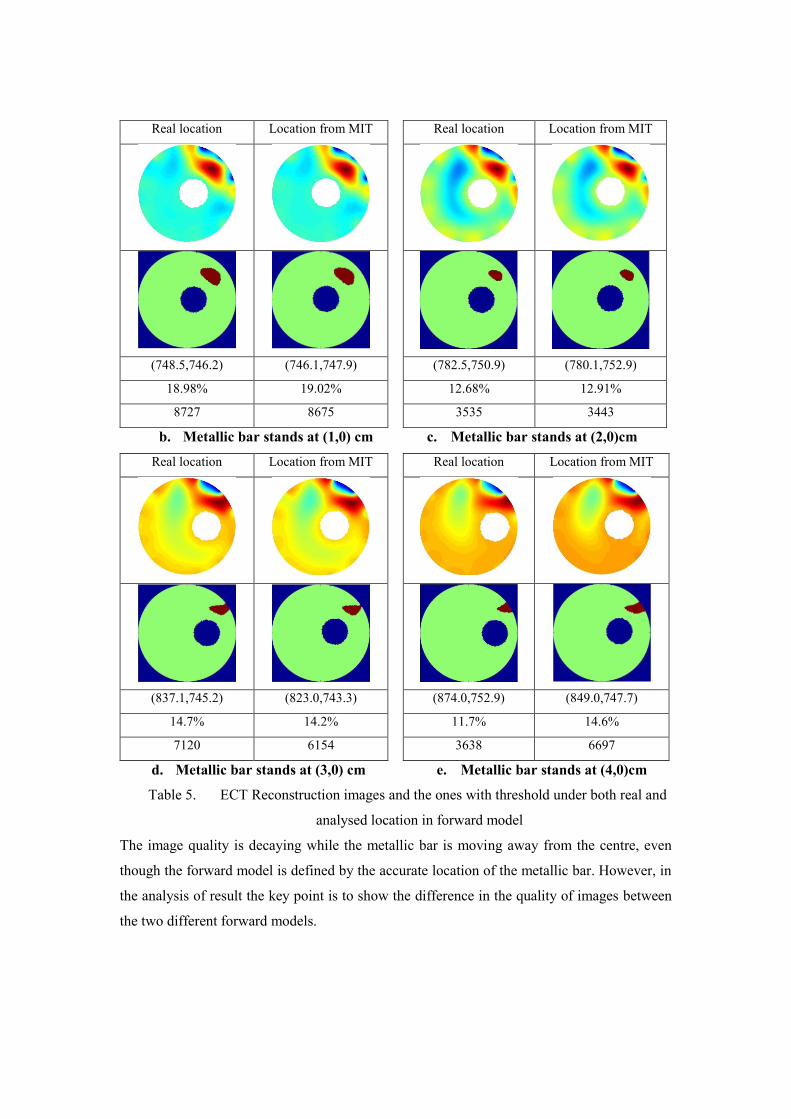
Real location Location from MIT

(748.5,746.2) (746.1,747.9)

18.98% 19.02%

8727 8675

Real location Location from MIT

(782.5,750.9) (780.1,752.9)

12.68% 12.91%

3535 3443

b. Metallic bar stands at (1,0) cm c. Metallic bar stands at (2,0)cm

Real location Location from MIT

(837.1,745.2) (823.0,743.3)

14.7% 14.2%

7120 6154

Real location Location from MIT

(874.0,752.9) (849.0,747.7)

11.7% 14.6%

3638 6697

d. Metallic bar stands at (3,0) cm e. Metallic bar stands at (4,0)cm

Table 5. ECT Reconstruction images and the ones with threshold under both real and

analysed location in forward model

The image quality is decaying while the metallic bar is moving away from the centre, even

though the forward model is defined by the accurate location of the metallic bar. However, in

the analysis of result the key point is to show the difference in the quality of images between

the two different forward models.

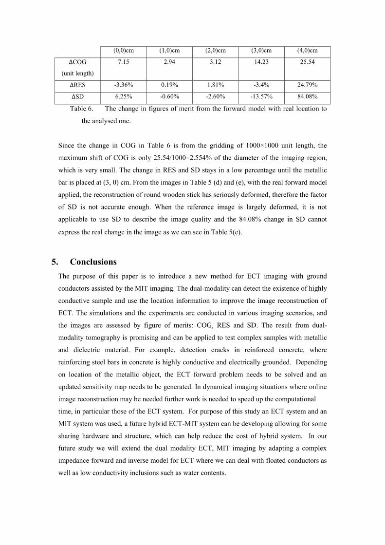
(0,0)cm (1,0)cm (2,0)cm (3,0)cm (4,0)cm

∆COG

(unit length)

7.15 2.94 3.12 14.23 25.54

∆RES -3.36% 0.19% 1.81% -3.4% 24.79%

∆SD 6.25% -0.60% -2.60% -13.57% 84.08%

Table 6. The change in figures of merit from the forward model with real location to

the analysed one.

Since the change in COG in Table 6 is from the gridding of 1000×1000 unit length, the

maximum shift of COG is only 25.54/1000=2.554% of the diameter of the imaging region,

which is very small. The change in RES and SD stays in a low percentage until the metallic

bar is placed at (3, 0) cm. From the images in Table 5 (d) and (e), with the real forward model

applied, the reconstruction of round wooden stick has seriously deformed, therefore the factor

of SD is not accurate enough. When the reference image is largely deformed, it is not

applicable to use SD to describe the image quality and the 84.08% change in SD cannot

express the real change in the image as we can see in Table 5(e).

5. Conclusions

The purpose of this paper is to introduce a new method for ECT imaging with ground

conductors assisted by the MIT imaging. The dual-modality can detect the existence of highly

conductive sample and use the location information to improve the image reconstruction of

ECT. The simulations and the experiments are conducted in various imaging scenarios, and

the images are assessed by figure of merits: COG, RES and SD. The result from dual-

modality tomography is promising and can be applied to test complex samples with metallic

and dielectric material. For example, detection cracks in reinforced concrete, where

reinforcing steel bars in concrete is highly conductive and electrically grounded. Depending

on location of the metallic object, the ECT forward problem needs to be solved and an

updated sensitivity map needs to be generated. In dynamical imaging situations where online

image reconstruction may be needed further work is needed to speed up the computational

time, in particular those of the ECT system. For purpose of this study an ECT system and an

MIT system was used, a future hybrid ECT-MIT system can be developing allowing for some

sharing hardware and structure, which can help reduce the cost of hybrid system. In our

future study we will extend the dual modality ECT, MIT imaging by adapting a complex

impedance forward and inverse model for ECT where we can deal with floated conductors as

well as low conductivity inclusions such as water contents.

References: 1. Jeanmeure, L.F.C., et al., Direct flow-pattern identification using electrical

capacitance tomography. Experimental Thermal and Fluid Science, 2002.

26(6-7): p. 763-773.

2. Jaworski, A.J. and T. Dyakowski, Application of electrical capacitance

tomography for measurement of gas-solids flow characteristics in a pneumatic

conveying system. Measurement Science & Technology, 2001. 12(8): p. 1109-

1119.

3. Soleimani, M., et al., Dynamic imaging in electrical capacitance tomography

and electromagnetic induction tomography using a Kalman filter.

Measurement Science & Technology, 2007. 18(11): p. 3287-3294.

4. Soleimani, M. and W.R.B. Lionheart, Nonlinear image reconstruction for

electrical capacitance tomography using experimental data. Measurement

Science & Technology, 2005. 16(10): p. 1987-1996.

5. Rimpilainen, V., et al., Electrical capacitance tomography as a monitoring

tool for high-shear mixing and granulation. Chemical Engineering Science,

2011. 66(18): p. 4090-4100.

6. Heikkinen, L., et al., Modelling of internal structures and electrodes in

electrical process tomography. Measurement Science and Technology, 2001.

12(8): p. 1012.

7. Griffiths, H., Magnetic induction tomography. Measurement Science &

Technology, 2001. 12(8): p. 1126-1131.

8. Qiu, C., B. Hoyle, and F. Podd, Engineering and application of a dual-

modality process tomography system. Flow Measurement and Instrumentation,

2007. 18(5): p. 247-254.

9. Wang, B., Z. Huang, and H. Li. Design of high-speed ECT and ERT system. in

Journal of Physics: Conference Series. 2009. IOP Publishing.

10. Yin, X., et al., Non-destructive evaluation of concrete using a capacitive

imaging technique: Preliminary modelling and experiments. Cement and

Concrete Research, 2010. 40(12): p. 1734-1743.

11. Adler, A., et al., GREIT: a unified approach to 2D linear EIT reconstruction

of lung images. Physiological measurement, 2009. 30(6): p. S35.

12. Yang, W.Q., Modelling of capacitance tomography sensors. Iee Proceedings-

Science Measurement and Technology, 1997. 144(5): p. 203-208.

13. Li, Y. and M. Soleimani, Imaging conductive materials with high frequency

electrical capacitance tomography. Measurement, 2013. 46(9): p. 3355-3361.

14. Yang, W.Q. and L.H. Peng, Image reconstruction algorithms for electrical

capacitance tomography. Measurement Science & Technology, 2003. 14(1):

p. R1-R13.

15. Korjenevsky, A., V. Cherepenin, and S. Sapetsky, Magnetic induction

tomography: experimental realization. Physiological Measurement, 2000.

21(1): p. 89-94.

16. Wei, H.-Y. and M. Soleimani, A Magnetic Induction Tomography System for

Prospective Industrial Processing Applications. Chinese Journal of Chemical

Engineering, 2012. 20(2): p. 406-410.

17. Bíró, O., Edge element formulations of eddy current problems. Computer

methods in applied mechanics and engineering, 1999. 169(3): p. 391-405.

18. Biro, O. and K. Preis, An edge finite element eddy current formulation using a

reduced magnetic and a current vector potential. Magnetics, IEEE

Transactions on, 2000. 36(5): p. 3128-3130.