Embed Size (px)
Citation preview
Printed in USA March 2000
NoticeHewlett-Packard to Agilent Technologies TransitionThis documentation supports a product that previously shipped under the Hewlett-Packard company brand name. The brand name has now been changed to AgilentTechnologies. The two products are functionally identical, only our name has changed. Thedocument still includes references to Hewlett-Packard products, some of which have beentransitioned to Agilent Technologies.
Programmer's Guide
HP 8753D Network Analyzer
Including Option 011
ABCDE
HP Part No. 08753-90256 Supersedes October 1995Printed in USA July 1997
Notice.
The information contained in this document is subject to change without notice.
Hewlett-Packard makes no warranty of any kind with regard to this material, including
but not limited to, the implied warranties of merchantability and �tness for a particular
purpose. Hewlett-Packard shall not be liable for errors contained herein or for incidental or
consequential damages in connection with the furnishing, performance, or use of this material.
c Copyright Hewlett-Packard Company 1994, 1995, 1997
All Rights Reserved. Reproduction, adaptation, or translation without prior written permission
is prohibited, except as allowed under the copyright laws.
1400 Fountaingrove Parkway, Santa Rosa, CA, 95403-1799, USA
Warranty
This Hewlett-Packard instrument product is warranted against defects in material and
workmanship for a period of one year from date of shipment. During the warranty period,
Hewlett-Packard Company will, at its option, either repair or replace products which prove to
be defective.
For warranty service or repair, this product must be returned to a service facility designated by
Hewlett-Packard. Buyer shall prepay shipping charges to Hewlett-Packard and Hewlett-Packard
shall pay shipping charges to return the product to Buyer. However, Buyer shall pay all
shipping charges, duties, and taxes for products returned to Hewlett-Packard from another
country.
Hewlett-Packard warrants that its software and �rmware designated by Hewlett-Packard for
use with an instrument will execute its programming instructions when properly installed on
that instrument. Hewlett-Packard does not warrant that the operation of the instrument, or
software, or �rmware will be uninterrupted or error-free.
Limitation of Warranty
The foregoing warranty shall not apply to defects resulting from improper or inadequate
maintenance by Buyer, Buyer-supplied software or interfacing, unauthorized modi�cation or
misuse, operation outside of the environmental speci�cations for the product, or improper
site preparation or maintenance.
NO OTHER WARRANTY IS EXPRESSED OR IMPLIED. HEWLETT-PACKARD SPECIFICALLY
DISCLAIMS THE IMPLIED WARRANTIES OF MERCHANTABILITY AND FITNESS FOR A
PARTICULAR PURPOSE.
Exclusive Remedies
THE REMEDIES PROVIDED HEREIN ARE BUYER'S SOLE AND EXCLUSIVE REMEDIES.
HEWLETT-PACKARD SHALL NOT BE LIABLE FOR ANY DIRECT, INDIRECT, SPECIAL,
INCIDENTAL, OR CONSEQUENTIAL DAMAGES, WHETHER BASED ON CONTRACT, TORT,
OR ANY OTHER LEGAL THEORY.
iii
2 Chapter 1
Contacting Agilent
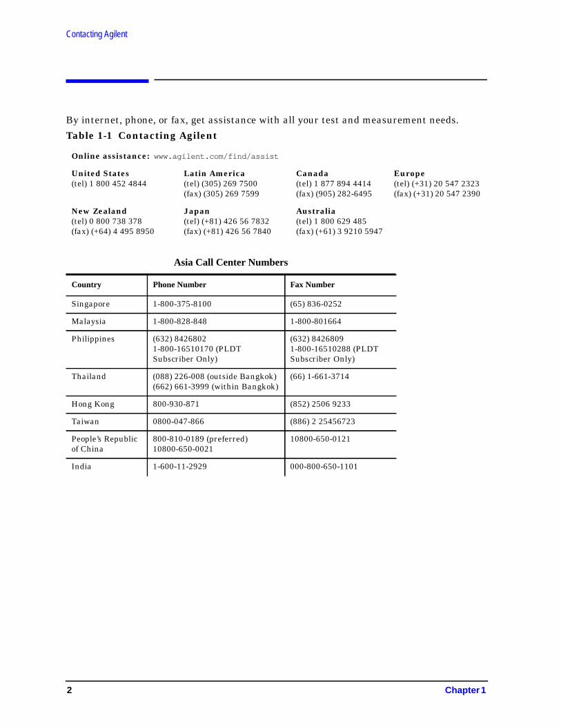
By internet, phone, or fax, get assistance with all your test and measurement needs.
Table 1-1 Contacting Agilent
Online assistance: www.agilent.com/find/assist
United States(tel) 1 800 452 4844
Latin America(tel) (305) 269 7500(fax) (305) 269 7599
Canada(tel) 1 877 894 4414(fax) (905) 282-6495
Europe(tel) (+31) 20 547 2323(fax) (+31) 20 547 2390
New Zealand(tel) 0 800 738 378(fax) (+64) 4 495 8950
Japan(tel) (+81) 426 56 7832(fax) (+81) 426 56 7840
Australia(tel) 1 800 629 485(fax) (+61) 3 9210 5947
Asia Call Center Numbers
Country Phone Number Fax Number
Singapore 1-800-375-8100 (65) 836-0252
Malaysia 1-800-828-848 1-800-801664
Philippines (632) 84268021-800-16510170 (PLDTSubscriber Only)
(632) 84268091-800-16510288 (PLDTSubscriber Only)
Thailand (088) 226-008 (outside Bangkok)(662) 661-3999 (within Bangkok)
(66) 1-661-3714
Hong Kong 800-930-871 (852) 2506 9233
Taiwan 0800-047-866 (886) 2 25456723
People’s Republicof China
800-810-0189 (preferred)10800-650-0021
10800-650-0121
India 1-600-11-2929 000-800-650-1101
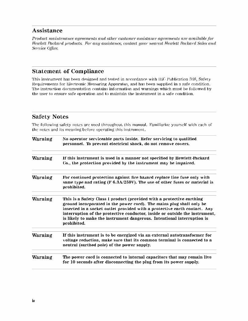
Assistance
Product maintenance agreements and other customer assistance agreements are available for
Hewlett-Packard products. For any assistance, contact your nearest Hewlett-Packard Sales and
Service O�ce.
Statement of Compliance
This instrument has been designed and tested in accordance with IEC Publication 348, Safety
Requirements for Electronic Measuring Apparatus, and has been supplied in a safe condition.
The instruction documentation contains information and warnings which must be followed by
the user to ensure safe operation and to maintain the instrument in a safe condition.
Safety Notes
The following safety notes are used throughout this manual. Familiarize yourself with each of
the notes and its meaning before operating this instrument.
Warning No operator serviceable parts inside. Refer servicing to quali�edpersonnel. To prevent electrical shock, do not remove covers.
Warning If this instrument is used in a manner not speci�ed by Hewlett-PackardCo., the protection provided by the instrument may be impaired.
Warning For continued protection against �re hazard replace line fuse only withsame type and rating (F 6.3A/250V). The use of other fuses or material isprohibited.
Warning This is a Safety Class I product (provided with a protective earthingground incorporated in the power cord). The mains plug shall only beinserted in a socket outlet provided with a protective earth contact. Anyinterruption of the protective conductor, inside or outside the instrument,is likely to make the instrument dangerous. Intentional interruption isprohibited.
Warning If this instrument is to be energized via an external autotransformer forvoltage reduction, make sure that its common terminal is connected to aneutral (earthed pole) of the power supply.
Warning The power cord is connected to internal capacitors that may remain livefor 10 seconds after disconnecting the plug from its power supply.
iv
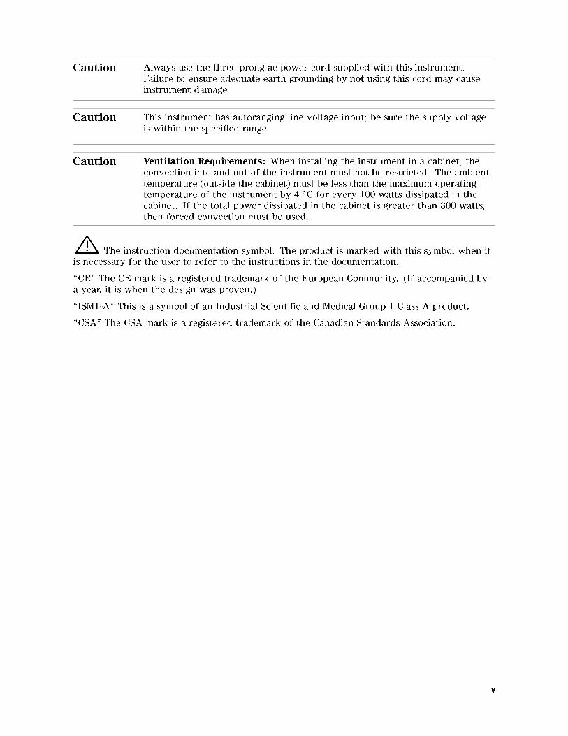
Caution Always use the three-prong ac power cord supplied with this instrument.
Failure to ensure adequate earth grounding by not using this cord may cause
instrument damage.
Caution This instrument has autoranging line voltage input; be sure the supply voltage
is within the speci�ed range.
Caution Ventilation Requirements: When installing the instrument in a cabinet, the
convection into and out of the instrument must not be restricted. The ambient
temperature (outside the cabinet) must be less than the maximum operating
temperature of the instrument by 4 �C for every 100 watts dissipated in the
cabinet. If the total power dissipated in the cabinet is greater than 800 watts,
then forced convection must be used.
L The instruction documentation symbol. The product is marked with this symbol when it
is necessary for the user to refer to the instructions in the documentation.
\CE" The CE mark is a registered trademark of the European Community. (If accompanied by
a year, it is when the design was proven.)
\ISM1-A" This is a symbol of an Industrial Scienti�c and Medical Group 1 Class A product.
\CSA" The CSA mark is a registered trademark of the Canadian Standards Association.
v

How to Use This Guide
This guide uses the following conventions:
�FRONT-PANEL KEY�This represents a key physically located on the instrument.NNNNNNNNNNNNNNNNNNNNNNNSoftkey This represents a \softkey," a key whose label is determined by the
instrument's �rmware.
Screen Text This represents text displayed on the instrument's screen.
vi
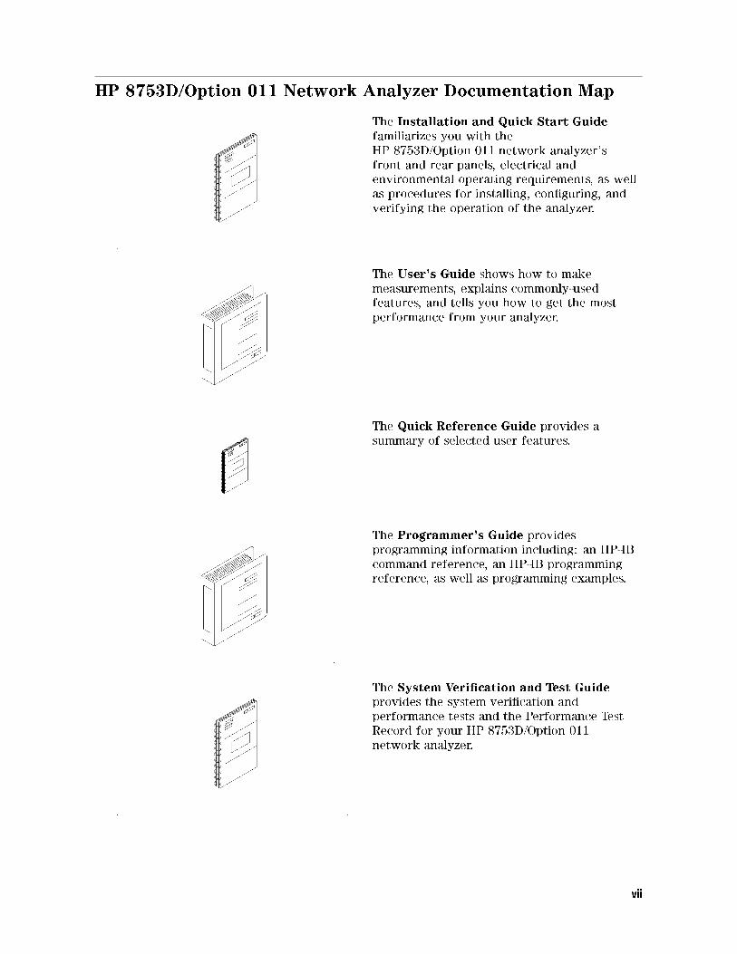
HP 8753D/Option 011 Network Analyzer Documentation Map
The Installation and Quick Start Guidefamiliarizes you with the
HP 8753D/Option 011 network analyzer's
front and rear panels, electrical and
environmental operating requirements, as well
as procedures for installing, con�guring, and
verifying the operation of the analyzer.
The User's Guide shows how to make
measurements, explains commonly-used
features, and tells you how to get the most
performance from your analyzer.
The Quick Reference Guide provides a
summary of selected user features.
The Programmer's Guide provides
programming information including: an HP-IB
command reference, an HP-IB programming
reference, as well as programming examples.
The System Veri�cation and Test Guideprovides the system veri�cation and
performance tests and the Performance Test
Record for your HP 8753D/Option 011
network analyzer.
vii

Contents
1. HP-IB Programming and Command ReferenceWhere to Look for More Information . . . . . . . . . . . . . . . . . . . . . 1-2
Analyzer Command Syntax . . . . . . . . . . . . . . . . . . . . . . . . . . 1-3
Code Naming Convention . . . . . . . . . . . . . . . . . . . . . . . . . 1-3
Valid Characters . . . . . . . . . . . . . . . . . . . . . . . . . . . . . . 1-4
Units . . . . . . . . . . . . . . . . . . . . . . . . . . . . . . . . . . . 1-4
Command Formats . . . . . . . . . . . . . . . . . . . . . . . . . . . . . 1-4
General Structure: . . . . . . . . . . . . . . . . . . . . . . . . . . . . 1-4
Syntax Types . . . . . . . . . . . . . . . . . . . . . . . . . . . . . . 1-5
HP-IB Operation . . . . . . . . . . . . . . . . . . . . . . . . . . . . . . . 1-6
Device Types . . . . . . . . . . . . . . . . . . . . . . . . . . . . . . . 1-6
Talker . . . . . . . . . . . . . . . . . . . . . . . . . . . . . . . . . . 1-6
Listener . . . . . . . . . . . . . . . . . . . . . . . . . . . . . . . . . 1-6
Controller . . . . . . . . . . . . . . . . . . . . . . . . . . . . . . . . 1-6
HP-IB Bus Structure . . . . . . . . . . . . . . . . . . . . . . . . . . . . 1-7
Data Bus . . . . . . . . . . . . . . . . . . . . . . . . . . . . . . . . 1-7
Handshake Lines . . . . . . . . . . . . . . . . . . . . . . . . . . . . 1-7
Control Lines . . . . . . . . . . . . . . . . . . . . . . . . . . . . . . 1-7
HP-IB Requirements . . . . . . . . . . . . . . . . . . . . . . . . . . . . 1-8
HP-IB Operational Capabilities . . . . . . . . . . . . . . . . . . . . . . . 1-9
HP-IB Status Indicators . . . . . . . . . . . . . . . . . . . . . . . . . 1-10
Bus Device Modes . . . . . . . . . . . . . . . . . . . . . . . . . . . . . 1-10
System-Controller Mode . . . . . . . . . . . . . . . . . . . . . . . . . 1-11
Talker/Listener Mode . . . . . . . . . . . . . . . . . . . . . . . . . . . 1-11
Pass-Control Mode . . . . . . . . . . . . . . . . . . . . . . . . . . . . 1-11
Analyzer Bus Modes . . . . . . . . . . . . . . . . . . . . . . . . . . . 1-11
Setting HP-IB Addresses . . . . . . . . . . . . . . . . . . . . . . . . . . 1-12
Response to HP-IB Meta-Messages (IEEE-488 Universal Commands) . . . . . . 1-12
Abort . . . . . . . . . . . . . . . . . . . . . . . . . . . . . . . . . . 1-12
Device Clear . . . . . . . . . . . . . . . . . . . . . . . . . . . . . . . 1-12
Local . . . . . . . . . . . . . . . . . . . . . . . . . . . . . . . . . . 1-12
Local Lockout . . . . . . . . . . . . . . . . . . . . . . . . . . . . . . 1-13
Parallel Poll . . . . . . . . . . . . . . . . . . . . . . . . . . . . . . . 1-13
Pass Control . . . . . . . . . . . . . . . . . . . . . . . . . . . . . . . 1-13
Remote . . . . . . . . . . . . . . . . . . . . . . . . . . . . . . . . . 1-13
Serial Poll . . . . . . . . . . . . . . . . . . . . . . . . . . . . . . . . 1-13
Trigger . . . . . . . . . . . . . . . . . . . . . . . . . . . . . . . . . 1-13
Analyzer Operation . . . . . . . . . . . . . . . . . . . . . . . . . . . . . 1-14
Operation Complete . . . . . . . . . . . . . . . . . . . . . . . . . . . . 1-14
Reading Analyzer Data . . . . . . . . . . . . . . . . . . . . . . . . . . . . 1-15
Output Queue . . . . . . . . . . . . . . . . . . . . . . . . . . . . . . . 1-15
Command Query . . . . . . . . . . . . . . . . . . . . . . . . . . . . . . 1-15
Identi�cation . . . . . . . . . . . . . . . . . . . . . . . . . . . . . . . 1-15
Output Syntax . . . . . . . . . . . . . . . . . . . . . . . . . . . . . . . 1-15
Marker data . . . . . . . . . . . . . . . . . . . . . . . . . . . . . . . . 1-16
Array-Data Formats . . . . . . . . . . . . . . . . . . . . . . . . . . . . 1-17
Contents-1
Trace-Data Transfers . . . . . . . . . . . . . . . . . . . . . . . . . . . . 1-19
Stimulus-Related Values . . . . . . . . . . . . . . . . . . . . . . . . . . 1-20
Data-Processing Chain . . . . . . . . . . . . . . . . . . . . . . . . . . . . 1-21
Data Arrays . . . . . . . . . . . . . . . . . . . . . . . . . . . . . . . . 1-21
Fast Data Transfer Commands . . . . . . . . . . . . . . . . . . . . . . . 1-23
Data Levels . . . . . . . . . . . . . . . . . . . . . . . . . . . . . . . . 1-23
Learn String and Calibration-Kit String . . . . . . . . . . . . . . . . . . . 1-24
Error Reporting . . . . . . . . . . . . . . . . . . . . . . . . . . . . . . . 1-25
Status Reporting . . . . . . . . . . . . . . . . . . . . . . . . . . . . . . 1-25
The Status Byte . . . . . . . . . . . . . . . . . . . . . . . . . . . . . . 1-27
The Event-Status Register and Event-Status Register B . . . . . . . . . . . . 1-27
Error Output . . . . . . . . . . . . . . . . . . . . . . . . . . . . . . . 1-28
Calibration . . . . . . . . . . . . . . . . . . . . . . . . . . . . . . . . . 1-28
Disk File Names . . . . . . . . . . . . . . . . . . . . . . . . . . . . . . 1-31
Using Key Codes . . . . . . . . . . . . . . . . . . . . . . . . . . . . . . 1-32
Key Select Codes Arranged by Front-Panel Hardkey . . . . . . . . . . . . . . 1-33
HP-IB Only Commands . . . . . . . . . . . . . . . . . . . . . . . . . . . . 1-57
Alphabetical Mnemonic Listing . . . . . . . . . . . . . . . . . . . . . . . . 1-64
2. HP BASIC Programming ExamplesIntroduction . . . . . . . . . . . . . . . . . . . . . . . . . . . . . . . . . 2-1
Required Equipment . . . . . . . . . . . . . . . . . . . . . . . . . . . . 2-2
Optional Equipment . . . . . . . . . . . . . . . . . . . . . . . . . . . 2-2
System Setup and HP-IB Veri�cation . . . . . . . . . . . . . . . . . . . . 2-2
HP 8753D Network Analyzer Instrument Control Using BASIC . . . . . . . . . 2-5
Command Structure in BASIC . . . . . . . . . . . . . . . . . . . . . . . 2-5
Command Query . . . . . . . . . . . . . . . . . . . . . . . . . . . . . . 2-6
Running the Program . . . . . . . . . . . . . . . . . . . . . . . . . . 2-7
Operation Complete . . . . . . . . . . . . . . . . . . . . . . . . . . . . 2-8
Running the Program . . . . . . . . . . . . . . . . . . . . . . . . . . 2-8
Preparing for Remote (HP-IB) Control . . . . . . . . . . . . . . . . . . . . 2-8
I/O Paths . . . . . . . . . . . . . . . . . . . . . . . . . . . . . . . . . 2-10
Measurement Process . . . . . . . . . . . . . . . . . . . . . . . . . . . . 2-11
Step 1. Setting Up the Instrument . . . . . . . . . . . . . . . . . . . . . 2-11
Step 2. Calibrating the Test Setup . . . . . . . . . . . . . . . . . . . . . 2-11
Step 3. Connecting the Device under Test . . . . . . . . . . . . . . . . . . 2-12
Step 4. Taking the Measurement Data . . . . . . . . . . . . . . . . . . . . 2-12
Step 5. Post-Processing the Measurement Data . . . . . . . . . . . . . . . 2-12
Step 6. Transferring the Measurement Data . . . . . . . . . . . . . . . . . 2-12
BASIC Programming Examples . . . . . . . . . . . . . . . . . . . . . . . . 2-13
Program Information . . . . . . . . . . . . . . . . . . . . . . . . . . . . 2-14
Analyzer Features Helpful in Developing Programming Routines . . . . . . . 2-14
Analyzer-Debug Mode . . . . . . . . . . . . . . . . . . . . . . . . . . 2-14
User-Controllable Sweep . . . . . . . . . . . . . . . . . . . . . . . . . 2-14
Example 1: Measurement Setup . . . . . . . . . . . . . . . . . . . . . . . 2-15
Example 1A: Setting Parameters . . . . . . . . . . . . . . . . . . . . . . 2-15
Running the Program . . . . . . . . . . . . . . . . . . . . . . . . . . 2-16
Example 1B: Verifying Parameters . . . . . . . . . . . . . . . . . . . . . 2-17
Running the Program . . . . . . . . . . . . . . . . . . . . . . . . . . 2-18
Example 2: Measurement Calibration . . . . . . . . . . . . . . . . . . . . . 2-19
Calibration Kits . . . . . . . . . . . . . . . . . . . . . . . . . . . . . . 2-19
Example 2A: S11 1-Port Calibration . . . . . . . . . . . . . . . . . . . . . 2-20
Running the Program . . . . . . . . . . . . . . . . . . . . . . . . . . 2-22
Example 2B: Full 2-Port Measurement Calibration . . . . . . . . . . . . . . 2-23
Running the Program . . . . . . . . . . . . . . . . . . . . . . . . . . 2-26
Contents-2
Example 2C: Adapter Removal Calibration . . . . . . . . . . . . . . . . . 2-27
Running the Program . . . . . . . . . . . . . . . . . . . . . . . . . . 2-28
Example 2D: Using Raw Data to Create a Calibration (Simmcal) . . . . . . . . 2-29
Running the Program . . . . . . . . . . . . . . . . . . . . . . . . . . 2-34
Example 2E: Take4 | Error Correction Processed on an External PC . . . . . 2-36
Overview . . . . . . . . . . . . . . . . . . . . . . . . . . . . . . . . 2-36
Using the Take4 Mode . . . . . . . . . . . . . . . . . . . . . . . . . . 2-36
Programming Example . . . . . . . . . . . . . . . . . . . . . . . . . . 2-37
Running the Program . . . . . . . . . . . . . . . . . . . . . . . . . . 2-42
Example 3: Measurement Data Transfer . . . . . . . . . . . . . . . . . . . 2-44
Trace-Data Formats and Transfers . . . . . . . . . . . . . . . . . . . . . 2-44
Example 3A: Data Transfer Using Markers . . . . . . . . . . . . . . . . . 2-45
Running the Program . . . . . . . . . . . . . . . . . . . . . . . . . . 2-46
Example 3B: Data Transfer Using FORM 4 (ASCII Transfer) . . . . . . . . . . 2-47
Running the Program . . . . . . . . . . . . . . . . . . . . . . . . . . 2-49
Example 3C: Data Transfer Using Floating-Point Numbers . . . . . . . . . . 2-50
Running the Program . . . . . . . . . . . . . . . . . . . . . . . . . . 2-51
Example 3D: Data Transfer Using Frequency-Array Information . . . . . . . 2-52
Running the Program . . . . . . . . . . . . . . . . . . . . . . . . . . 2-54
Example 3E: Data Transfer Using FORM 1 (Internal-Binary Format) . . . . . . 2-55
Running the Program . . . . . . . . . . . . . . . . . . . . . . . . . . 2-56
Example 4: Measurement Process Synchronization . . . . . . . . . . . . . . . 2-57
Status Reporting . . . . . . . . . . . . . . . . . . . . . . . . . . . . . . 2-57
Example 4A: Using the Error Queue . . . . . . . . . . . . . . . . . . . . 2-58
Running the Program . . . . . . . . . . . . . . . . . . . . . . . . . . 2-59
Example 4B: Generating Interrupts . . . . . . . . . . . . . . . . . . . . . 2-61
Running the Program . . . . . . . . . . . . . . . . . . . . . . . . . . 2-63
Example 4C: Power Meter Calibration . . . . . . . . . . . . . . . . . . . . 2-64
Running the Program . . . . . . . . . . . . . . . . . . . . . . . . . . 2-67
Example 5: Network Analyzer System Setups . . . . . . . . . . . . . . . . . 2-68
Saving and Recalling Instrument States . . . . . . . . . . . . . . . . . . . 2-68
Example 5A: Using the Learn String . . . . . . . . . . . . . . . . . . . . 2-68
Running the Program . . . . . . . . . . . . . . . . . . . . . . . . . . 2-69
Example 5B: Reading Calibration Data . . . . . . . . . . . . . . . . . . . 2-70
Running the Program . . . . . . . . . . . . . . . . . . . . . . . . . . 2-72
Example 5C: Saving and Restoring the Analyzer Instrument State . . . . . . . 2-73
Running the Program . . . . . . . . . . . . . . . . . . . . . . . . . . 2-75
Example 6: Limit-Line Testing . . . . . . . . . . . . . . . . . . . . . . . . 2-76
Using List-Frequency Mode . . . . . . . . . . . . . . . . . . . . . . . . . 2-76
Example 6A: Setting Up a List-Frequency Sweep . . . . . . . . . . . . . . 2-76
Running the Program . . . . . . . . . . . . . . . . . . . . . . . . . . 2-78
Example 6B: Selecting a Single Segment from a Table of Segments . . . . . . 2-79
Running the Program . . . . . . . . . . . . . . . . . . . . . . . . . . 2-81
Using Limit Lines to Perform PASS/FAIL Tests . . . . . . . . . . . . . . . . 2-81
Example 6C: Setting Up Limit Lines . . . . . . . . . . . . . . . . . . . . . 2-82
Running the Program . . . . . . . . . . . . . . . . . . . . . . . . . . 2-84
Example 6D: Performing PASS/FAIL Tests While Tuning . . . . . . . . . . . 2-85
Running the Program . . . . . . . . . . . . . . . . . . . . . . . . . . 2-87
Example 7: Report Generation . . . . . . . . . . . . . . . . . . . . . . . . 2-88
Example 7A1: Operation Using Talker/Listener Mode . . . . . . . . . . . . 2-88
Running the Program . . . . . . . . . . . . . . . . . . . . . . . . . . 2-89
Example 7A2: Controlling Peripherals Using Pass-Control Mode . . . . . . . . 2-90
Running the Program . . . . . . . . . . . . . . . . . . . . . . . . . . 2-92
Example 7A3: Printing with the Serial Port . . . . . . . . . . . . . . . . . 2-93
Running the Program . . . . . . . . . . . . . . . . . . . . . . . . . . 2-94
Contents-3
Example 7B: Plotting to a File and Transferring the File Data to a Plotter . . . 2-95
Running the Program . . . . . . . . . . . . . . . . . . . . . . . . . . 2-96
Utilizing PC-Graphics Applications Using the Plot File . . . . . . . . . . . . 2-97
Example 7C: Reading ASCII Disk Files to the Instrument Controller's Disk File 2-97
Running the Program . . . . . . . . . . . . . . . . . . . . . . . . . . 2-101
Example 8: Mixer Measurements . . . . . . . . . . . . . . . . . . . . . . . 2-102
Example 8A: Comparison of Two Mixers | Group Delay, Amplitude or Phase . 2-102
Running the Program . . . . . . . . . . . . . . . . . . . . . . . . . . 2-105
Limit Line and Data Point Special Functions . . . . . . . . . . . . . . . . . . 2-106
Overview . . . . . . . . . . . . . . . . . . . . . . . . . . . . . . . . . 2-107
Example Display of Limit Lines . . . . . . . . . . . . . . . . . . . . . . 2-109
Limit Segments . . . . . . . . . . . . . . . . . . . . . . . . . . . . . 2-110
Output Results . . . . . . . . . . . . . . . . . . . . . . . . . . . . . . 2-111
Constants Used Throughout This Document . . . . . . . . . . . . . . . . . 2-112
Output Limit Test Pass/Fail Status Per Limit Segment . . . . . . . . . . . . . 2-113
Output Pass/Fail Status for All Segments . . . . . . . . . . . . . . . . . . 2-114
Example Program of OUTPSEGAF Using BASIC . . . . . . . . . . . . . . 2-114
Output Minimum and Maximum Point Per Limit Segment . . . . . . . . . . . 2-116
Output Minimum and Maximum Point For All Segments . . . . . . . . . . . 2-117
Example Program of OUTPSEGAM Using BASIC . . . . . . . . . . . . . . 2-118
Output Data Per Point . . . . . . . . . . . . . . . . . . . . . . . . . . . 2-119
Output Data Per Range of Points . . . . . . . . . . . . . . . . . . . . . . 2-120
Output Limit Pass/Fail by Channel . . . . . . . . . . . . . . . . . . . . . 2-121
Index
Contents-4
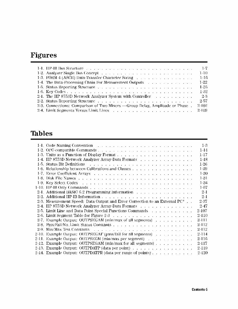
Figures
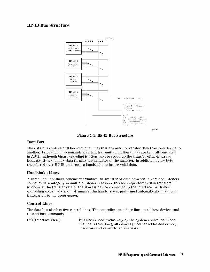
1-1. HP-IB Bus Structure . . . . . . . . . . . . . . . . . . . . . . . . . . . . 1-7
1-2. Analyzer Single Bus Concept . . . . . . . . . . . . . . . . . . . . . . . . 1-10
1-3. FORM 4 (ASCII) Data-Transfer Character String . . . . . . . . . . . . . . . 1-16
1-4. The Data-Processing Chain For Measurement Outputs . . . . . . . . . . . . 1-22
1-5. Status Reporting Structure . . . . . . . . . . . . . . . . . . . . . . . . . 1-25
1-6. Key Codes . . . . . . . . . . . . . . . . . . . . . . . . . . . . . . . . . 1-32
2-1. The HP 8753D Network Analyzer System with Controller . . . . . . . . . . 2-3
2-2. Status Reporting Structure . . . . . . . . . . . . . . . . . . . . . . . . . 2-57
2-3. Connections: Comparison of Two Mixers | Group Delay, Amplitude or Phase . 2-102
2-4. Limit Segments Versus Limit Lines . . . . . . . . . . . . . . . . . . . . . 2-109
Tables
1-1. Code Naming Convention . . . . . . . . . . . . . . . . . . . . . . . . . 1-3
1-2. OPC-compatible Commands . . . . . . . . . . . . . . . . . . . . . . . . . 1-14
1-3. Units as a Function of Display Format . . . . . . . . . . . . . . . . . . . . 1-17
1-4. HP 8753D Network Analyzer Array-Data Formats . . . . . . . . . . . . . . 1-18
1-5. Status Bit De�nitions . . . . . . . . . . . . . . . . . . . . . . . . . . . 1-26
1-6. Relationship between Calibrations and Classes . . . . . . . . . . . . . . . . 1-29
1-7. Error Coe�cient Arrays . . . . . . . . . . . . . . . . . . . . . . . . . . 1-30
1-8. Disk File Names . . . . . . . . . . . . . . . . . . . . . . . . . . . . . . 1-31
1-9. Key Select Codes . . . . . . . . . . . . . . . . . . . . . . . . . . . . . 1-34
1-10. HP-IB Only Commands . . . . . . . . . . . . . . . . . . . . . . . . . . . 1-57
2-1. Additional BASIC 6.2 Programming Information . . . . . . . . . . . . . . . 2-1
2-2. Additional HP-IB Information . . . . . . . . . . . . . . . . . . . . . . . . 2-1
2-3. Measurement Speed: Data Output and Error Correction to an External PC* . . 2-37
2-4. HP 8753D Network Analyzer Array-Data Formats . . . . . . . . . . . . . . 2-47
2-5. Limit Line and Data Point Special Functions Commands . . . . . . . . . . . 2-107
2-6. Limit Segment Table for Figure 2-3 . . . . . . . . . . . . . . . . . . . . . 2-110
2-7. Example Output: OUTPSEGAM (min/max of all segments) . . . . . . . . . . 2-111
2-8. Pass/Fail/No Limit Status Constants . . . . . . . . . . . . . . . . . . . . . 2-112
2-9. Min/Max Test Constants . . . . . . . . . . . . . . . . . . . . . . . . . . 2-112
2-10. Example Output: OUTPSEGAF (pass/fail for all segments) . . . . . . . . . . 2-114
2-11. Example Output: OUTPSEGM (min/max per segment) . . . . . . . . . . . . 2-116
2-12. Example Output: OUTPSEGAM (min/max for all segments) . . . . . . . . . . 2-117
2-13. Example Output: OUTPDATP (data per point) . . . . . . . . . . . . . . . . 2-119
2-14. Example Output: OUTPDATPR (data per range of points) . . . . . . . . . . . 2-120
Contents-5

1
HP-IB Programming and Command Reference
This chapter is a reference for operation of the network analyzer under HP-IB control. You
should already be familiar with making measurements with the analyzer. Information about the
HP-IB commands is organized as follows:
Analyzer Command Syntax
Code Naming Convention
Valid Characters
Units
Command Formats
HP-IB Operation
Device Types
HP-IB Bus Structure
HP-IB Requirements
HP-IB Operational Capabilities
Bus Device Modes
Setting HP-IB Addresses
Response to HP-IB Meta-Messages (IEEE-488 Universal Commands)
Analyzer Operation-Complete Commands
Reading Analyzer Data
Output Queue
Command Query
Identi�cation
Output Syntax
Marker Data
Array-Data Formats
Trace-Data Transfers
Stimulus-Related Values
Data Processing Chain
Data Arrays
Fast Data Transfer Commands
Data Levels
Learn String and Calibration Kit String
HP-IB Programming and Command Reference 1-1
Error Reporting
Status Reporting
The Status Byte
The Event-Status Register and Event-Status Register B
Error Output
Calibration
Disk File Names
Using Key Codes
Key Select Codes Arranged by Front-Panel Hardkey
HP-IB Only Commands
Alphabetical Mnemonic Listing
For information about manual operation of the analyzer, refer to the HP 8753D Network
Analyzer User's Guide.
Where to Look for More Information
Additional information covering many of the topics discussed in this chapter is located in the
following:
Tutorial Description of the Hewlett-Packard Interface Bus, presents a description and
discussion of all aspects of the HP-IB. A thorough overview of all technical details as a broad
tutorial. HP publication, HP part number 5021-1927.
IEEE Standard Digital Interface for Programmable Instrumentation ANSI/IEEE std
488.1-1987 contains detailed information on IEEE-488 operation. Published by the Institute
of Electrical and Electronics Engineers, Inc., 345 East 47th Street, New York,
New York 10017.
Chapter 2, \HP BASIC Programming Examples," includes programming examples in
HP BASIC.
1-2 HP-IB Programming and Command Reference
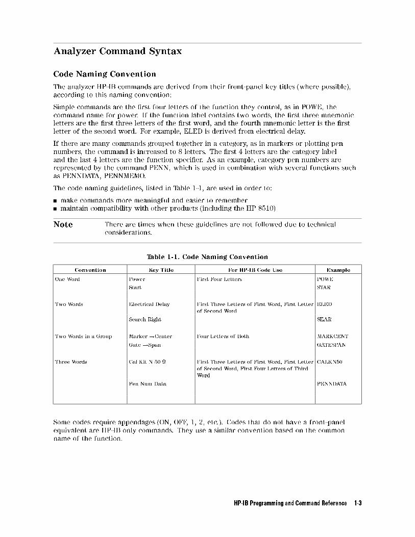
Analyzer Command Syntax
Code Naming Convention
The analyzer HP-IB commands are derived from their front-panel key titles (where possible),
according to this naming convention:
Simple commands are the �rst four letters of the function they control, as in POWE, the
command name for power. If the function label contains two words, the �rst three mnemonic
letters are the �rst three letters of the �rst word, and the fourth mnemonic letter is the �rst
letter of the second word. For example, ELED is derived from electrical delay.
If there are many commands grouped together in a category, as in markers or plotting pen
numbers, the command is increased to 8 letters. The �rst 4 letters are the category label
and the last 4 letters are the function speci�er. As an example, category pen numbers are
represented by the command PENN, which is used in combination with several functions such
as PENNDATA, PENNMEMO.
The code naming guidelines, listed in Table 1-1, are used in order to:
make commands more meaningful and easier to remember
maintain compatibility with other products (including the HP 8510)
Note There are times when these guidelines are not followed due to technical
considerations.
Table 1-1. Code Naming Convention
Convention Key Title For HP-IB Code Use Example
One Word Power First Four Letters POWE
Start STAR
Two Words Electrical Delay First Three Letters of First Word, First Letter
of Second Word
ELED
Search Right SEAR
Two Words in a Group Marker !Center Four Letters of Both MARKCENT
Gate !Span GATESPAN
Three Words Cal Kit N 50 First Three Letters of First Word, First Letter
of Second Word, First Four Letters of Third
Word
CALKN50
Pen Num Data PENNDATA
Some codes require appendages (ON, OFF, 1, 2, etc.). Codes that do not have a front-panel
equivalent are HP-IB only commands. They use a similar convention based on the common
name of the function.
HP-IB Programming and Command Reference 1-3
Valid Characters
The analyzer accepts the following ASCII characters:
letters
numbers
decimal points
+/�semicolons (;)
quotation marks (")
carriage returns (CR)
linefeeds (LF)
Both upper- and lower-case letters are acceptable. Carriage returns, leading zeros, spaces, and
unnecessary terminators are ignored, except for those within a command or appendage. If the
analyzer does not recognize a character as appropriate, it generates a syntax error message and
recovers at the next terminator.
Units
The analyzer can input and output data in basic units such as Hz, dB, seconds, etc.
S Seconds HZ Hertz
V Volts DB dB or dBm
Input data is assumed to be in basic units (see above) unless one of the following units is used
(upper and lower case are equivalent):
MS Milliseconds KHZ Kilohertz
US Microseconds MHZ Megahertz
NS Nanoseconds GHZ Gigahertz
PS Picoseconds FS Femtoseconds
Command Formats
The HP-IB commands accepted by the analyzer can be grouped into �ve input-syntax types.
The analyzer does not distinguish between upper- and lower-case letters.
General Structure:
The general syntax structure is: [code][appendage][data][unit][terminator]
The individual sections of the syntax code are explained below.
[code] The root mnemonic (these codes are described in the \Alphabetical Mnemonic
Listing" later in this chapter.)
[appendage] A quali�er attached to the root mnemonic. Possible appendages are ON or
OFF (toggle a function ON or OFF), or integers, which specify one capability
out of several. There can be no spaces or symbols between the code and the
appendage.
1-4 HP-IB Programming and Command Reference
[data] A single operand used by the root mnemonic, usually to set the value of a
function. The data can be a number or a character string. Numbers are
accepted as integers or decimals, with power of ten speci�ed by E (for
example, STAR 0.2E+10; sets the start frequency to 2 GHz). Character strings
must be enclosed by double quotation marks.
For example:A title string using RMB BASIC would look like:
OUTPUT 716;"TITL"""Unit1""";"
where the �rst two "" are an escape so that RMB BASIC will interpret the
third " properly.
[unit] The units of the operand, if applicable. If no units are speci�ed, the analyzer
assumes the basic units as described above. The data is entered into the
function when either units or a terminator are received.
[terminator] Indicates the end of the command, enters the data, and switches the
active-entry area OFF. A semicolon (;) is the recommended terminator.
Terminators are not necessary for the analyzer to interpret commands
correctly, but in the case of a syntax error, the analyzer will attempt to recover
at the next terminator. The analyzer also interprets line feeds and HP-IB END
OR IDENTIFY (EOI) messages as terminators.
Syntax Types
The speci�c syntax types are:
SYNTAX TYPE 1: [code] [terminator]
These are simple action commands that require no complementary information, such as
AUTO; (autoscales the active channel).
SYNTAX TYPE 2: [code][appendage][terminator]
These are simple action commands requiring limited customization, such as CORRON; and
CORROFF; (error correction ON or OFF) or RECA1;, RECA2;, RECA3; (recall register 1, 2, 3).
There can be no characters or symbols between the code and the appendage.
Note In the following cases: CLEAREG[D], RECAREG[D], SAVEREG[D], and EG[D],
[D] must be 2 characters. For example, CLEAREG01; will execute, while
CLEAREG1; will generate a syntax error.
SYNTAX TYPE 3: [code] [data] [unit][terminator]
These are data-input commands such as STAR 1.0 GHZ; (set the start frequency to 1 GHz).
SYNTAX TYPE 4: [code] [appendage] [data] [terminator]
These are titling and marker commands that have an appendage, such as TITR1 "STATE1"
(title register 1 STATE1), TITR2 "TEST2" (title register 2 TEST2).
QUERY SYNTAX: [code][?]
To query a front-panel-equivalent function, append a question mark (?) to the root
mnemonic. (For example, POWE?, AVERO?, or REAL?.) To query commands with integer
appendages, place the question mark after the appendage.
HP-IB Programming and Command Reference 1-5
HP-IB Operation
The Hewlett-Packard Interface Bus (HP-IB) is Hewlett-Packard's hardware, software,
documentation, and support for IEEE 488.2 and IEC-625 worldwide standards for interfacing
instruments. This interface allows you to operate the analyzer and peripherals in two methods:
by an external system controller
by the network analyzer in system-controller mode
Device Types
The HP-IB employs a party-line bus structure in which up to 15 devices can be connected
on one contiguous bus. The interface consists of 16 signal lines and 8 ground lines within a
shielded cable. With this cabling system, many di�erent types of devices including instruments,
computers, power meters, plotters, printers, and disk drives can be connected in parallel.
Every HP-IB device must be capable of performing one or more of the following interface
functions:
Talker
A talker is a device capable of transmitting device-dependent data when addressed to talk.
There can be only one active talker at any given time. Examples of this type of device include:
power meters
disk drives
voltmeters
counters
tape readers
The network analyzer is a talker when it sends trace data or marker information over the bus.
Listener
A listener is a device capable of receiving device-dependent data over the interface when
addressed to listen. There can be as many as 14 listeners connected to the interface at any
given time. Examples of this type of device include:
printers
power supplies
signal generators
The network analyzer is a listener when it is controlled over the bus by a system controller.
Controller
A controller is de�ned as a device capable of:
1. managing the operation of the bus
2. addressing talkers and listeners
There can be only one active controller on the interface at any time. Examples of controllers
include desktop computers, minicomputers, workstations, and the network analyzer. In a
multiple-controller system, active control can be passed between controllers, but there can
only be one system controller connected to the interface. The system controller acts as the
master and can regain active control at any time. The analyzer is an active controller when it
plots, prints, or stores to an external disk drive in the pass-control mode. The analyzer is also a
system controller when it is operating in the system controller mode.
1-6 HP-IB Programming and Command Reference
HP-IB Bus Structure
Figure 1-1. HP-IB Bus Structure
Data Bus
The data bus consists of 8 bi-directional lines that are used to transfer data from one device to
another. Programming commands and data transmitted on these lines are typically encoded
in ASCII, although binary encoding is often used to speed up the transfer of large arrays.
Both ASCII- and binary-data formats are available to the analyzer. In addition, every byte
transferred over HP-IB undergoes a handshake to insure valid data.
Handshake Lines
A three-line handshake scheme coordinates the transfer of data between talkers and listeners.
To insure data integrity in multiple-listener transfers, this technique forces data transfers
to occur at the transfer rate of the slowest device connected to the interface. With most
computing controllers and instruments, the handshake is performed automatically, making it
transparent to the programmer.
Control Lines
The data bus also has �ve control lines. The controller uses these lines to address devices and
to send bus commands.
IFC (Interface Clear) This line is used exclusively by the system controller. When
this line is true (low), all devices (whether addressed or not)
unaddress and revert to an idle state.
HP-IB Programming and Command Reference 1-7
ATN (Attention) The active controller uses this line to de�ne whether
the information on the data bus is command-oriented or
data-oriented. When this line is true (low), the bus is in the
command mode, and the data lines carry bus commands. When
this line is false (high), the bus is in the data mode, and the
data lines carry device-dependent instructions or data.
SRQ (Service Request) This line is set true (low) when a device requests service
and the active controller services the requesting device. The
network analyzer can be enabled to pull the SRQ line for a
variety of reasons such as requesting control of the interface,
for the purposes of printing, plotting, or accessing a disk.
REN (Remote Enable) This line is used exclusively by the system controller. When this
line is set true (low), the bus is in the remote mode, and devices
are addressed by the controller to either listen or talk. When
the bus is in remote mode and a device is addressed, it receives
instructions from the system controller via HP-IB rather than
from its front panel (pressing �Local� returns the device tofront-panel operation). When this line is set false (high), the
bus and all of the connected devices return to local operation.
EOI (End or Identify) This line is used by a talker to indicate the last data byte in a
multiple-byte transmission, or by an active controller to initiate
a parallel-poll sequence. The analyzer recognizes the EOI line
as a terminator, and it pulls the EOI line with the last byte of a
message output (data, markers, plots, prints, error messages).
The analyzer does not respond to parallel poll.
HP-IB Requirements
Number of Interconnected Devices: 15 maximum.
Interconnection Path Maximum Cable Length: 20 meters maximum or 2 meters per device
(whichever is less).
Message Transfer Scheme: Byte serial, bit parallel asynchronous data
transfer using a 3-line handshake system.
Data Rate: Maximum of 1 megabyte-per-second over the
speci�ed distances with tri-state drivers. Actual
data rate depends on the transfer rate of the
slowest device connected to the bus.
Address Capability: Primary addresses: 31 talk, 31 listen. A
maximum of 1 talker and 14 listeners can be
connected to the interface at given time.
Multiple-Controller Capability: In systems with more than one controller (such
as this instrument), only one controller can be
active at any given time. The active controller
can pass control to another controller, but only
the system controller can assume unconditional
control. Only one system controller is allowed.
1-8 HP-IB Programming and Command Reference
HP-IB Operational Capabilities
On the network analyzer's rear panel, next to the HP-IB connector, there is a list of HP-IB
device subsets as de�ned by the IEEE 488.2 standard. The analyzer has the following
capabilities:
SH1 Full-source handshake.
AH1 Full-acceptor handshake.
T6 Basic talker, answers serial poll, unaddresses if MLA is issued. No talk-only mode.
L4 Basic listener, unaddresses if MTA is issued. No listen-only mode.
SR1 Complete service request (SRQ) capabilities.
RL1 Complete remote/local capability including local lockout.
PP0 Does not respond to parallel poll.
DC1 Complete device clear.
DT1 Responds to a Group Execute Trigger (GET) in the hold-trigger mode.
C1,C2,C3 System controller capabilities in system-controller mode.
C10 Pass control capabilities in pass-control mode.
E2 Tri-state drivers.
LE0 No extended listener capabilities.
TE0 No extended talker capabilities.
These codes are completely explained in the IEEE Std 488 documents, published by the
Institute of Electrical and Electronic Engineers, Inc., 345 East 47th Street, New York,
New York 11017.
HP-IB Programming and Command Reference 1-9
HP-IB Status Indicators
When the analyzer is connected to other instruments over the HP-IB, the HP-IB status
indicators illuminate to display the current status of the analyzer. The HP-IB status indicators
are located in the instrument-state function block on the front panel of the network analyzer.
R = Remote Operation
L = Listen mode
T = Talk mode
S = Service request (SRQ) asserted by the analyzer
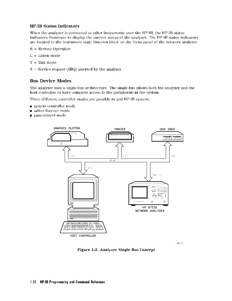
Bus Device Modes
The analyzer uses a single-bus architecture. The single bus allows both the analyzer and the
host controller to have complete access to the peripherals in the system.
Three di�erent controller modes are possible in and HP-IB system:
system-controller mode
talker/listener mode
pass-control mode
Figure 1-2. Analyzer Single Bus Concept
1-10 HP-IB Programming and Command Reference
System-Controller Mode
This mode allows the analyzer to control peripherals directly in a stand-alone environment
(without an external controller). This mode can only be selected manually from the
analyzer's front panel. It can only be used if no active computer or instrument controller is
connected to the system via HP-IB. If an attempt is made to set the network analyzer to the
system-controller mode when another controller is connected to the interface, the following
message is displayed on the analyzer's display screen:
"ANOTHER SYSTEM CONTROLLER ON HP-IB BUS"
The analyzer must be set to the system-controller mode in order to access peripherals from the
front panel. In this mode, the analyzer can directly control peripherals (plotters, printers, disk
drives, power meters, etc.) and the analyzer may plot, print, store on disk or perform power
meter functions.
Note Do not attempt to use this mode for programming. HP recommends using an
external instrument controller when programming. See the following section,
\Talker/Listener Mode."
Talker/Listener Mode
This is the mode that is normally used for remote programming of the analyzer. In
talker/listener mode, the analyzer and all peripheral devices are controlled from an external
instrument controller. The controller can command the analyzer to talk and other devices
to listen. The analyzer and peripheral devices cannot talk directly to each other unless the
computer sets up a data path between them. This mode allows the analyzer to act as either
a talker or a listener, as required by the controlling computer for the particular operation in
progress.
Pass-Control Mode
This mode allows the computer to control the analyzer via HP-IB (as with the talker/listener
mode), but also allows the analyzer to take control of the interface in order to plot, print, or
access a disk. During an analyzer-controlled peripheral operation, the host computer is free to
perform other internal tasks (i.e. data or display manipulation) while the analyzer is controlling
the bus. After the analyzer-controlled task is completed, the analyzer returns control to the
system controller.
Note Performing an instrument preset does not a�ect the selected bus mode,
although the bus mode will return to talker/listener mode if the line power is
cycled.
Note \Speci�cations and Measurement Uncertainties" in the HP 8753D Network
Analyzer User's Guide provides information on setting the correct bus mode
from the front-panel menu.
Analyzer Bus Modes
As discussed earlier, under HP-IB control, the analyzer can operate in one of three modes:
talker/listener, pass-control, or system-controller mode.
In talker/listener mode, the analyzer behaves as a simple device on the bus. While in this
mode, the analyzer can make a plot or print using the OUTPPLOT; or OUTPPRIN; commands.
The analyzer will wait until it is addresses to talk by the system controller and then dump
the display to a plotter/printer that the system controller has addressed to listen. Use of the
commands PLOT; and PRINALL; require control to be passed to another controller.
HP-IB Programming and Command Reference 1-11
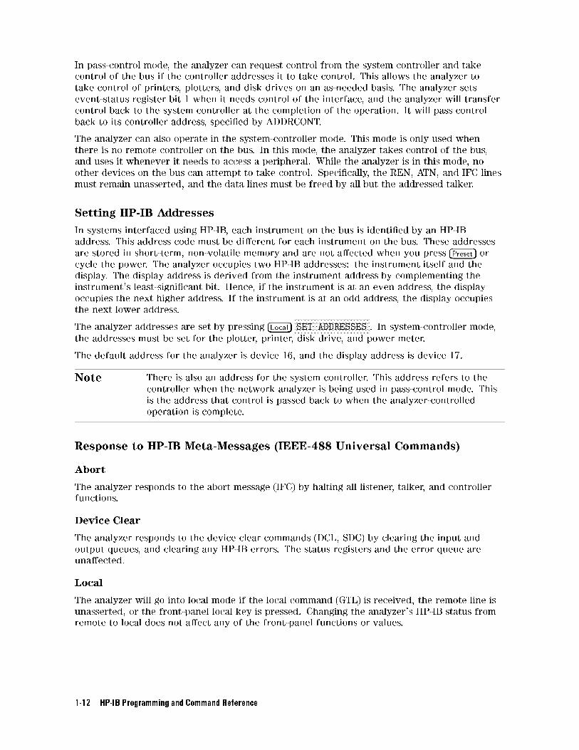
In pass-control mode, the analyzer can request control from the system controller and take
control of the bus if the controller addresses it to take control. This allows the analyzer to
take control of printers, plotters, and disk drives on an as-needed basis. The analyzer sets
event-status register bit 1 when it needs control of the interface, and the analyzer will transfer
control back to the system controller at the completion of the operation. It will pass control
back to its controller address, speci�ed by ADDRCONT.
The analyzer can also operate in the system-controller mode. This mode is only used when
there is no remote controller on the bus. In this mode, the analyzer takes control of the bus,
and uses it whenever it needs to access a peripheral. While the analyzer is in this mode, no
other devices on the bus can attempt to take control. Speci�cally, the REN, ATN, and IFC lines
must remain unasserted, and the data lines must be freed by all but the addressed talker.
Setting HP-IB Addresses
In systems interfaced using HP-IB, each instrument on the bus is identi�ed by an HP-IB
address. This address code must be di�erent for each instrument on the bus. These addresses
are stored in short-term, non-volatile memory and are not a�ected when you press �Preset� orcycle the power. The analyzer occupies two HP-IB addresses: the instrument itself and the
display. The display address is derived from the instrument address by complementing the
instrument's least-signi�cant bit. Hence, if the instrument is at an even address, the display
occupies the next higher address. If the instrument is at an odd address, the display occupies
the next lower address.
The analyzer addresses are set by pressing �Local�NNNNNNNNNNNNNNNNNNNNNNNNNNNNNNNNNNNNNNNNNSET ADDRESSES . In system-controller mode,
the addresses must be set for the plotter, printer, disk drive, and power meter.
The default address for the analyzer is device 16, and the display address is device 17.
Note There is also an address for the system controller. This address refers to the
controller when the network analyzer is being used in pass-control mode. This
is the address that control is passed back to when the analyzer-controlled
operation is complete.
Response to HP-IB Meta-Messages (IEEE-488 Universal Commands)
Abort
The analyzer responds to the abort message (IFC) by halting all listener, talker, and controller
functions.
Device Clear
The analyzer responds to the device clear commands (DCL, SDC) by clearing the input and
output queues, and clearing any HP-IB errors. The status registers and the error queue are
una�ected.
Local
The analyzer will go into local mode if the local command (GTL) is received, the remote line is
unasserted, or the front-panel local key is pressed. Changing the analyzer's HP-IB status from
remote to local does not a�ect any of the front-panel functions or values.
1-12 HP-IB Programming and Command Reference
Local Lockout
If the analyzer receives the local-lockout command (LLO) while it is in remote mode, it will
disable the entire front panel except for the line power switch. A local-lockout condition can
only be cleared by releasing the remote line, although the local command (GTL) will place the
instrument temporarily in local mode.
Parallel Poll
The analyzer does not respond to parallel-poll con�gure (PPC) or parallel-poll uncon�gure (PPU)
messages.
Pass Control
If the analyzer is in pass-control mode, is addressed to talk, and receives the take-control
command (TCT), from the system control it will take active control of the bus. If the analyzer
is not requesting control, it will immediately pass control to the system controller's address.
Otherwise, the analyzer will execute the function for which it sought control of the bus and
then pass control back to the system controller.
Remote
The analyzer will go into remote mode when the remote line is asserted and the analyzer is
addressed to listen. While the analyzer is held in remote mode, all front-panel keys (with the
exception of �Local�) are disabled. Changing the analyzer's HP-IB status from remote to local
does not a�ect any front-panel settings or values.
Serial Poll
The analyzer will respond to a serial poll with its status byte, as de�ned in the \Status
Reporting" section of this chapter. To initiate the serial-poll sequence, address the analyzer to
talk and issue a serial-poll enable command (SPE). Upon receiving this command, the analyzer
will return its status byte. End the sequence by issuing a serial-poll disable command (SPD). A
serial poll does not a�ect the value of the status byte, and it does not set the instrument to
remote mode.
Trigger
In hold mode, the analyzer responds to device trigger by taking a single sweep. The analyzer
responds only to selected-device trigger (SDT). This means that it will not respond to group
execute-trigger (GET) unless it is addressed to listen. The analyzer will not respond to GET if it
is not in hold mode.
HP-IB Programming and Command Reference 1-13
Analyzer Operation
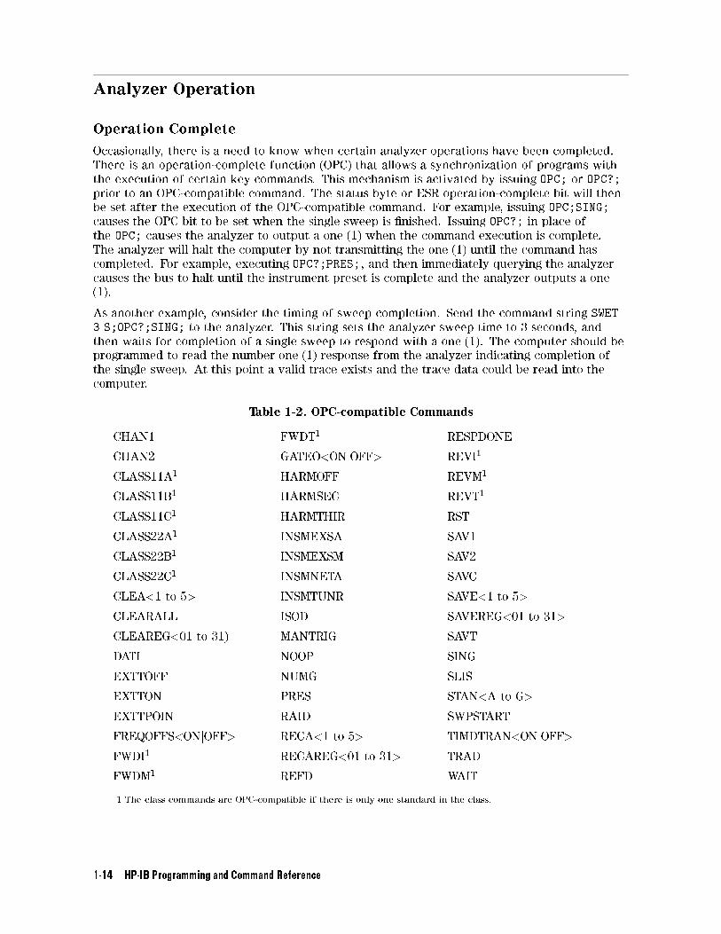
Operation Complete
Occasionally, there is a need to know when certain analyzer operations have been completed.
There is an operation-complete function (OPC) that allows a synchronization of programs with
the execution of certain key commands. This mechanism is activated by issuing OPC; or OPC?;
prior to an OPC-compatible command. The status byte or ESR operation-complete bit will then
be set after the execution of the OPC-compatible command. For example, issuing OPC;SING;
causes the OPC bit to be set when the single sweep is �nished. Issuing OPC?; in place of
the OPC; causes the analyzer to output a one (1) when the command execution is complete.
The analyzer will halt the computer by not transmitting the one (1) until the command has
completed. For example, executing OPC?;PRES;, and then immediately querying the analyzer
causes the bus to halt until the instrument preset is complete and the analyzer outputs a one
(1).
As another example, consider the timing of sweep completion. Send the command string SWET
3 S;OPC?;SING; to the analyzer. This string sets the analyzer sweep time to 3 seconds, and
then waits for completion of a single sweep to respond with a one (1). The computer should be
programmed to read the number one (1) response from the analyzer indicating completion of
the single sweep. At this point a valid trace exists and the trace data could be read into the
computer.
Table 1-2. OPC-compatible Commands
CHAN1
CHAN2
CLASS11A1
CLASS11B1
CLASS11C1
CLASS22A1
CLASS22B1
CLASS22C1
CLEA<1 to 5>
CLEARALL
CLEAREG<01 to 31)
DATI
EXTTOFF
EXTTON
EXTTPOIN
FREQOFFS<ONjOFF>
FWDI1
FWDM1
FWDT1
GATEO<ONjOFF>
HARMOFF
HARMSEC
HARMTHIR
INSMEXSA
INSMEXSM
INSMNETA
INSMTUNR
ISOD
MANTRIG
NOOP
NUMG
PRES
RAID
RECA<1 to 5>
RECAREG<01 to 31>
REFD
RESPDONE
REVI1
REVM1
REVT1
RST
SAV1
SAV2
SAVC
SAVE<1 to 5>
SAVEREG<01 to 31>
SAVT
SING
SLIS
STAN<A to G>
SWPSTART
TIMDTRAN<ONjOFF>
TRAD
WAIT
1 The class commands are OPC-compatible if there is only one standard in the class.
1-14 HP-IB Programming and Command Reference
Reading Analyzer Data
Output Queue
Whenever an output-data command is received, the analyzer puts the data into the output
queue (or bu�er) where it is held until the system controller outputs the next read command.
The queue, however, is only one event long: the next output-data command will overwrite the
data already in the queue. Therefore, it is important to read the output queue immediately
after every query or data request from the analyzer.
Command Query
All instrument functions can be queried to �nd the current ON/OFF state or value. For
instrument state commands, append the question mark character (?) to the command to
query the state of the functions. Suppose the operator has changed the power level from the
analyzer's front panel. The computer can ascertain the new power level using the analyzer's
command-query function. If a question mark is appended to the root of a command, the
analyzer will output the value of that function. For instance, POWE 7 DB; sets the source power
to 7 dB, and POWE?; outputs the current RF source power at the test port. When the analyzer
receives POWE?;, it prepares to transmit the current RF source power level. This condition
illuminates the analyzer front-panel talk light (T). In this case, the analyzer transmits the
output power to the controller.
ON/OFF commands can be also be queried. The reply is a one (1) if the function is ON or a
zero (0) if it is OFF. For example, if a command controls an active function that is underlined
on the analyzer display, querying that command yields a one (1) if the command is underlined
or a zero (0) if it is not. As another example, there are nine options on the format menu and
only one option is underlined at a time. Only the underlined option will return a one when
queried.
For instance, send the command string DUAC?; to the analyzer. If dual-channel display is
switched ON, the analyzer will return a one (1) to the instrument controller.
Similarly, to determine if phase is being measured and displayed, send the command string
PHAS?; to the analyzer. In this case, the analyzer will return a one (1) if phase is currently
being displayed. Since the command only applies to the active channel, the response to the
PHAS?; query depends on which channel is active.
Identi�cation
The analyzer's response to IDN?; is HEWLETT PACKARD,87NND,0,X.XX where 87NND is the
model number of the instrument and X.XX is the �rmware revision of the instrument.
The analyzer also has the capability to output its serial number with the command OUTPSERN;,
and to output its installed options with the command OUTPOPTS;.
Output Syntax
The following three types of data are transmitted by the analyzer in ASCII format:
response to query
certain output commands
ASCII oating-point (FORM 4) array transfers
HP-IB Programming and Command Reference 1-15
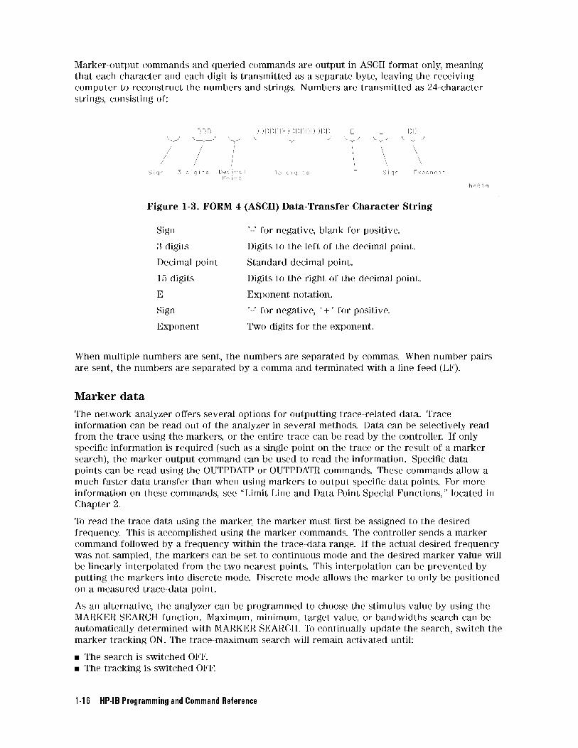
Marker-output commands and queried commands are output in ASCII format only, meaning
that each character and each digit is transmitted as a separate byte, leaving the receiving
computer to reconstruct the numbers and strings. Numbers are transmitted as 24-character
strings, consisting of:
Figure 1-3. FORM 4 (ASCII) Data-Transfer Character String
Sign '-' for negative, blank for positive.
3 digits Digits to the left of the decimal point.
Decimal point Standard decimal point.
15 digits Digits to the right of the decimal point.
E Exponent notation.
Sign '-' for negative, '+' for positive.
Exponent Two digits for the exponent.
When multiple numbers are sent, the numbers are separated by commas. When number pairs
are sent, the numbers are separated by a comma and terminated with a line feed (LF).
Marker data
The network analyzer o�ers several options for outputting trace-related data. Trace
information can be read out of the analyzer in several methods. Data can be selectively read
from the trace using the markers, or the entire trace can be read by the controller. If only
speci�c information is required (such as a single point on the trace or the result of a marker
search), the marker output command can be used to read the information. Speci�c data
points can be read using the OUTPDATP or OUTPDATR commands. These commands allow a
much faster data transfer than when using markers to output speci�c data points. For more
information on these commands, see \Limit Line and Data Point Special Functions," located in
Chapter 2.
To read the trace data using the marker, the marker must �rst be assigned to the desired
frequency. This is accomplished using the marker commands. The controller sends a marker
command followed by a frequency within the trace-data range. If the actual desired frequency
was not sampled, the markers can be set to continuous mode and the desired marker value will
be linearly interpolated from the two nearest points. This interpolation can be prevented by
putting the markers into discrete mode. Discrete mode allows the marker to only be positioned
on a measured trace-data point.
As an alternative, the analyzer can be programmed to choose the stimulus value by using the
MARKER SEARCH function. Maximum, minimum, target value, or bandwidths search can be
automatically determined with MARKER SEARCH. To continually update the search, switch the
marker tracking ON. The trace-maximum search will remain activated until:
The search is switched OFF.
The tracking is switched OFF.
1-16 HP-IB Programming and Command Reference
All markers are switched OFF.
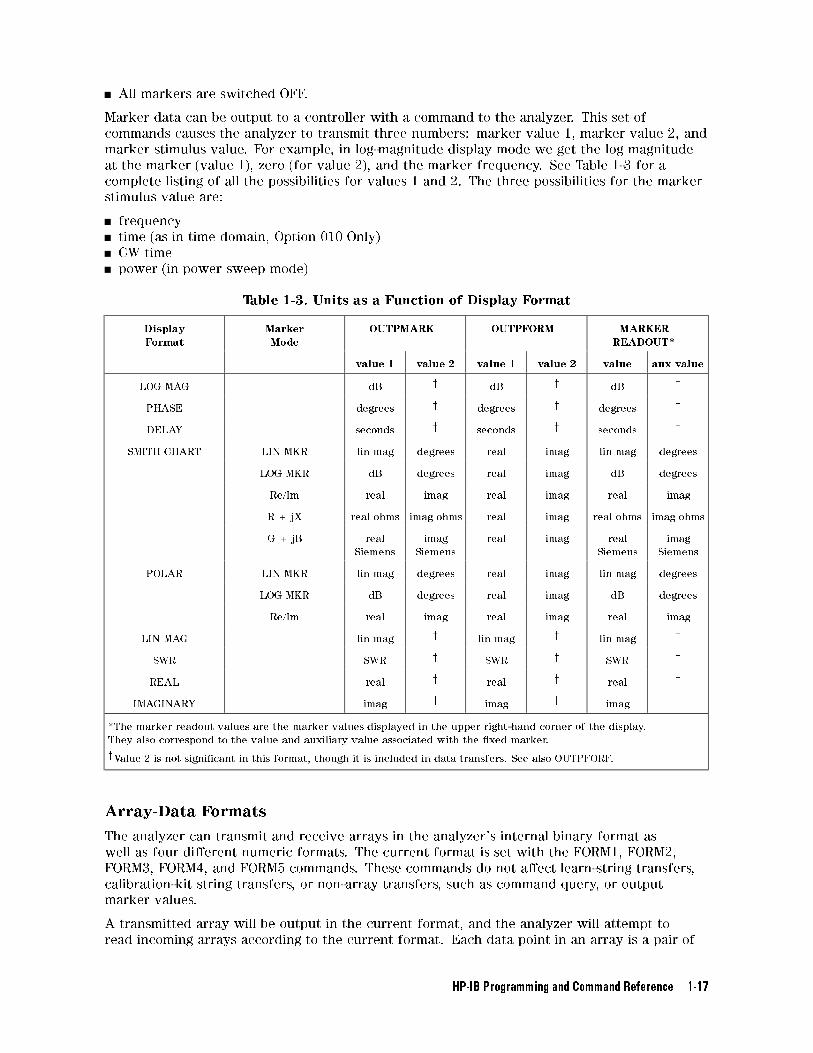
Marker data can be output to a controller with a command to the analyzer. This set of
commands causes the analyzer to transmit three numbers: marker value 1, marker value 2, and
marker stimulus value. For example, in log-magnitude display mode we get the log magnitude
at the marker (value 1), zero (for value 2), and the marker frequency. See Table 1-3 for a
complete listing of all the possibilities for values 1 and 2. The three possibilities for the marker
stimulus value are:
frequency
time (as in time domain, Option 010 Only)
CW time
power (in power sweep mode)
Table 1-3. Units as a Function of Display Format
Display
Format
Marker
Mode
OUTPMARK OUTPFORM MARKER
READOUT*
value 1 value 2 value 1 value 2 value aux value
LOG MAG dB y dB y dB y
PHASE degrees y degrees y degrees y
DELAY seconds y seconds y seconds y
SMITH CHART LIN MKR lin mag degrees real imag lin mag degrees
LOG MKR dB degrees real imag dB degrees
Re/Im real imag real imag real imag
R + jX real ohms imag ohms real imag real ohms imag ohms
G + jB real
Siemens
imag
Siemens
real imag real
Siemens
imag
Siemens
POLAR LIN MKR lin mag degrees real imag lin mag degrees
LOG MKR dB degrees real imag dB degrees
Re/Im real imag real imag real imag
LIN MAG lin mag y lin mag y lin mag y
SWR SWR y SWR y SWR y
REAL real y real y real y
IMAGINARY imag y imag y imag y
*The marker readout values are the marker values displayed in the upper right-hand corner of the display.
They also correspond to the value and auxiliary value associated with the �xed marker.
yValue 2 is not signi�cant in this format, though it is included in data transfers. See also OUTPFORF.
Array-Data Formats
The analyzer can transmit and receive arrays in the analyzer's internal binary format as
well as four di�erent numeric formats. The current format is set with the FORM1, FORM2,
FORM3, FORM4, and FORM5 commands. These commands do not a�ect learn-string transfers,
calibration-kit string transfers, or non-array transfers, such as command query, or output
marker values.
A transmitted array will be output in the current format, and the analyzer will attempt to
read incoming arrays according to the current format. Each data point in an array is a pair of
HP-IB Programming and Command Reference 1-17
numbers, usually a real/imaginary pair. The number of data points in each array is the same as
the number of points in the current sweep.
The �ve formats are described below:
FORM1 The analyzer's internal binary format, 6 bytes-per-data point. The array is
preceded by a four-byte header. The �rst two bytes represent the string "#A",
the standard block header. The second two bytes are an integer representing
the number of bytes in the block to follow. FORM 1 is best applied when rapid
data transfers, not to be modi�ed by the computer nor interpreted by the user,
are required.
FORM2 IEEE 32-bit oating-point format, 8 bytes-per-data point. The data is preceded
by the same header as in FORM1. Each number consists of a 1-bit sign, an 8-bit
biased exponent, and a 23-bit mantissa. FORM 2 is the format of choice if your
computer supports single-precision oating-point numbers.
FORM3 IEEE 64-bit oating-point format, 16 bytes-per-data point. The data is
preceded by the same header as in FORM 1. Each number consists of a 1-bit
sign, an 11-bit biased exponent, and a 52-bit mantissa. This format may be
used with double-precision oating-point numbers. No additional precision
is available in the analyzer data, but FORM 3 may be a convenient form for
transferring data to your computer.
FORM4 ASCII oating-point format. The data is transmitted as ASCII numbers, as
described in \Output Syntax".
There is no header. The analyzer always uses FORM 4 to transfer data that is
not related to array transfers (i.e. marker responses and instrument settings).
FORM5 PC-DOS 32-bit oating-point format with 4 bytes-per-number, 8 bytes-per-data
point. The data is preceded by the same header as in FORM 1. The byte order
is reversed to comply with PC-DOS formats. If you are using a PC-based
controller, FORM 5 is the most e�ective format to use.
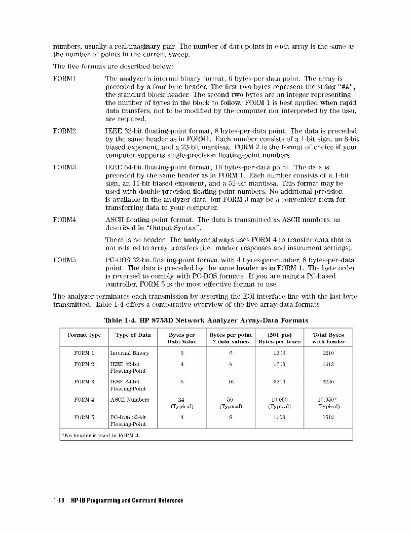
The analyzer terminates each transmission by asserting the EOI interface line with the last byte
transmitted. Table 1-4 o�ers a comparative overview of the �ve array-data formats.
Table 1-4. HP 8753D Network Analyzer Array-Data Formats
Format type Type of Data Bytes per
Data Value
Bytes per point
2 data values
(201 pts)
Bytes per trace
Total Bytes
with header
FORM 1 Internal Binary 3 6 1206 1210
FORM 2 IEEE 32-bit
Floating-Point
4 8 1608 1612
FORM 3 IEEE 64-bit
Floating-Point
8 16 3216 3220
FORM 4 ASCII Numbers 24
(Typical)
50
(Typical)
10,050
(Typical)
10,050*
(Typical)
FORM 5 PC-DOS 32-bit
Floating-Point
4 8 1608 1612
*No header is used in FORM 4.
1-18 HP-IB Programming and Command Reference
Trace-Data Transfers
Transferring trace-data from the analyzer using an instrument controller can be divided into
three steps:
1. allocating an array to receive and store the data
2. commanding the analyzer to transmit the data
3. accepting the transferred data
Data residing in the analyzer is always stored in pairs for each data point (to accommodate
real/imaginary pairs). Hence, the receiving array has to be two elements wide, and as deep
as the number of points in the array being transferred. Memory space for the array must be
declared before any data can be transferred from the analyzer to the computer.
As mentioned earlier, the analyzer can transmit data over HP-IB in �ve di�erent formats. The
type of format a�ects what kind of data array is declared (real or integer), because the format
determines what type of data is transferred. Examples of data transfers using di�erent formats
are discussed \Example 3: Measurement Data Transfer." For information on the various types
of data that can be obtained (raw data, error-corrected data, etc.), see \Data Levels," located
later in this chapter.
For information on transferring trace-data by selected points, see \Limit Line and Data Point
Special Functions," located in Chapter 2.
Note \Example 7C: Reading ASCII Disk Files to the Instrument Controller's Disk
File," located in Chapter 2, explains how to access disk �les from a computer.
HP-IB Programming and Command Reference 1-19
Stimulus-Related Values
Frequency-related values are calculated for the analyzer display. The start and stop
frequencies or center and span frequencies of the selected frequency range are available to the
programmer.
In a linear frequency range, the frequency values can be easily calculated because the trace
data points are equally spaced across the trace. Relating the data from a linear frequency
sweep to frequency can be done by querying the start frequency, the frequency span, and the
number of points in the trace.
Given that information, the frequency of point n in a linear-frequency sweep is represented by
the equation:
F=Start frequency + (n�1) � Span/(Points�1)
In most cases, this is an easy solution for determining the related frequency value that
corresponds with a data point. This technique is illustrated in \Example 3B: Data Transfer
Using FORM 4 (ASCII Format)."
When using log sweep or a list-frequency sweep, the points are not evenly spaced over the
frequency range of the sweep. In these cases, an e�ective way of determining the frequencies
of the current sweep is to use the OUTPLIML command. Although this command is normally
used for limit lines, it can also be used to identify all of the frequency points in a sweep. Limit
lines do not need to be on in order to read the frequencies directly out of the instrument
with the OUTPLIML command. Refer to example 3D, \Data Transfer Using Frequency Array
Information."
Note Another method of identifying all of the frequency points in a sweep is to
use the marker commands MARKBUCKx and OUTPMARK in a FOR NEXT
programming loop that corresponds to the number of points in the sweep.
MARKBUCKx places a marker at a point in the sweep, where x is the number
of the point in a sweep, and OUTPMARK outputs the stimulus value as part of
the marker data.
1-20 HP-IB Programming and Command Reference
Data-Processing Chain
This section describes the manner in which the analyzer processes measurement data. It
includes information on data arrays, common output commands, data levels, the learn string,
and the calibration kit string.
Data Arrays
Figure 1-4 shows the di�erent kinds of data available within the instrument:
pre-raw measured data
raw measured data
error-corrected data
formatted data
trace memory
calibration coe�cients
Trace memory can be directly output to a controller with OUTPMEMO;, but it cannot be directly
transmitted back.
HP-IB Programming and Command Reference 1-21
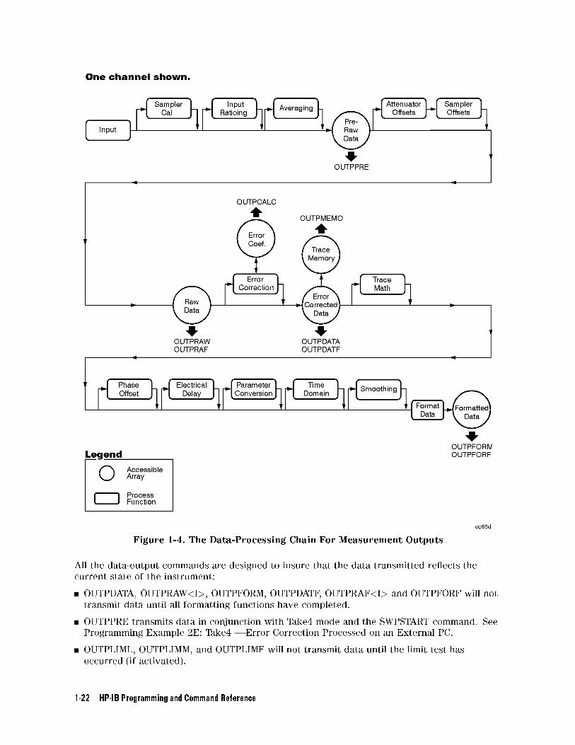
Figure 1-4. The Data-Processing Chain For Measurement Outputs
All the data-output commands are designed to insure that the data transmitted re ects the
current state of the instrument:
OUTPDATA, OUTPRAW<I>, OUTPFORM, OUTPDATF, OUTPRAF<I> and OUTPFORF will not
transmit data until all formatting functions have completed.
OUTPPRE transmits data in conjunction with Take4 mode and the SWPSTART command. See
Programming Example 2E: Take4 | Error Correction Processed on an External PC.
OUTPLIML, OUTPLIMM, and OUTPLIMF will not transmit data until the limit test has
occurred (if activated).
1-22 HP-IB Programming and Command Reference
OUTPMARK will activate a marker if a marker is not already selected. It will also insure that
any current marker searches have been completed before transmitting data.
OUTPMSTA insures that the statistics have been calculated for the current trace before
transmitting data. If the statistics are not activated, it will activate the statistics long enough
to update the current values before deactivating the statistics.
OUTPMWID insures that a bandwidth search has been executed for the current trace before
transmitting data. If the bandwidth-search function is not activated, it will activate the
bandwidth-search function long enough to update the current values before switching OFF
the bandwidth-search functions.
Fast Data Transfer Commands
The HP 8753D has four distinct fast data transfer commands. These commands circumvent
the internal \byte handler" routine and output trace dumps as block data. In other words, the
analyzer outputs the entire array without allowing any process swapping to occur. FORM4,
ASCII data transfer times are not a�ected by these routines. However, there are speed
improvements with binary data formats. The following is a description of the four fast data
transfer commands:
OUTPDATF outputs the error corrected data from the active channel in the current output
format. This data may be input to the analyzer using the INPUDATA command.
OUTPFORF outputs the formatted display trace array from the active channel in the current
output format, but only the �rst number in each of the OUTPFORM data pairs is actually
transferred for the display formatsNNNNNNNNNNNNNNNNNNNNNNNLOG MAG ,
NNNNNNNNNNNNNNNNNPHASE , group
NNNNNNNNNNNNNNNNNDELAY ,
NNNNNNNNNNNNNNNNNNNNNNNLIN MAG ,
NNNNNNNNNNNSWR ,
NNNNNNNNNNNNNNREAL
andNNNNNNNNNNNNNNIMAG inary. Because the data array does not contain the second value for these display
formats, the INPUFORM command may not be used to re-input the data back into the
analyzer. The second value may not be signi�cant in some display formats (see Table 1-4),
thus eliminating it reduces the number of bytes transferred.
OUTPMEMF outputs the memory trace from the active channel. The data is in real/imaginary
pairs, and, as such, may be input back into the memory trace using INPUDATA or INPUFORM
followed by the DATI command.
OUTPRAF<I> outputs the raw measurement data trace. The data may be input back into the
memory trace using the INPURAW<I> command.
Data Levels
Di�erent levels of data can be read out of the instrument. Refer to the data-processing chain
in Figure 1-4. The following list describes the di�erent types of data that are available from
the network analyzer.
Pre-raw data This is the raw data without sampler correction or attenuator
o�sets applied. With raw o�sets turned o�, the calibration
coe�cients generated can be transferred to an external
controller and used with the data gathered using the
OUTPPRE[1-4] commands. See Programming Example 2E: Take4
| Error Correction Processed on an External Computer. The
four arrays refer to S11, S21, S12 and S22 respectively. These
four arrays are available only if 2-port correction or Take4
mode is on. This data is represented in real/imaginary pairs.
Raw data The basic measurement data, re ecting the stimulus
parameters, IF averaging, and IF bandwidth. If a full 2-port
measurement calibration is activated, there are actually four
HP-IB Programming and Command Reference 1-23
raw arrays kept: one for each raw S-parameter. The data can
be output to a controller with the commands OUTPRAW1,
OUTPRAW2, OUTPRAW3, OUTPRAW4. Normally, only raw 1
is available, and it holds the current parameter. If a 2-port
measurement calibration is active, the four arrays refer to
S11, S21, S12, and S22 respectively. This data is represented in
real/imaginary pairs.
Error-corrected data This is the raw data with error-correction applied. The array
represents the currently measured parameter, and is stored in
real/imaginary pairs. The error-corrected data can be output to
a controller with the OUTPDATA; command. The OUTPMEMO;
command reads the trace memory, if available. The trace
memory also contains error-corrected data. Note that neither
raw nor error-corrected data re ect such post-processing
functions as electrical-delay o�set, trace math, or time-domain
gating.
Formatted data This is the array of data actually being displayed. It re ects
all post-processing functions such as electrical delay and time
domain. The units of the array output depend on the current
display format. See Table 1-3 for the various units de�ned as a
function of display format.
Calibration coe�cients The results of a measurement calibration are arrays containing
calibration coe�cients. These calibration coe�cients are then
used in the error-correction routines. Each array corresponds to
a speci�c error term in the error model. The HP 8753D Network
Analyzer User's details which error coe�cients are used for
speci�c calibration types, as well as the arrays those coe�cients
can be found in. Not all calibration types use all 12 arrays. The
data is stored as real/imaginary pairs.
Generally, formatted data is the most useful of the �ve data levels, because it is the same
information the operator sees on the display. However if post-processing is unnecessary
(e.g. possibly in cases involving smoothing), error-corrected data may be more desirable.
Error-corrected data also a�ords the user the opportunity to input the data to the network
analyzer and apply post-processing at another time.
Learn String and Calibration-Kit String
The learn string is a summary of the instrument state. It includes all the front-panel settings,
the limit-test tables, and the list-frequency table for the current instrument state. It does not
include calibration data or the information stored in the save/recall registers.
The learn string can be output to a controller with the OUTPLEAS; command, which commands
the analyzer to start transmitting the binary string. The string has a �xed length for a given
�rmware revision. The array has the same header as in FORM 1. See Example 5, \Using the
Learn String."
The calibration kit includes a set of key characteristics of the calibration standards used to
determine the calibration accuracy. There are default kits for several di�erent connector
types. There is also space for a user-de�ned calibration kit. The command OUTPCALK outputs
the currently active calibration kit as a binary string in FORM 1. As with the learn string, the
calibration-kit string has a �xed length for a given �rmware revision.
1-24 HP-IB Programming and Command Reference
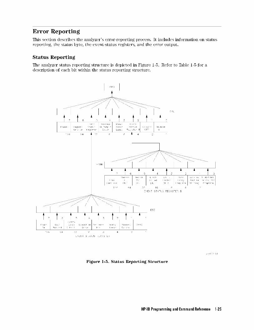
Error Reporting
This section describes the analyzer's error-reporting process. It includes information on status
reporting, the status byte, the event-status registers, and the error output.
Status Reporting
The analyzer status reporting structure is depicted in Figure 1-5. Refer to Table 1-5 for a
description of each bit within the status reporting structure.
Figure 1-5. Status Reporting Structure
HP-IB Programming and Command Reference 1-25
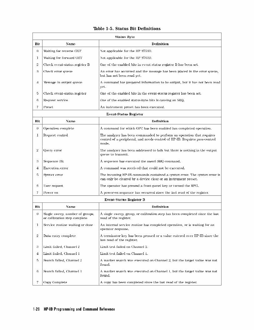
Table 1-5. Status Bit De�nitions
Status Byte
Bit Name De�nition
0 Waiting for reverse GET Not applicable for the HP 8753D.
1 Waiting for forward GET Not applicable for the HP 8753D.
2 Check event-status register B One of the enabled bits in event status register B has been set.
3 Check error queue An error has occurred and the message has been placed in the error queue,
but has not been read yet.
4 Message in output queue A command has prepared information to be output, but it has not been read
yet.
5 Check event-status register One of the enabled bits in the event-status register has been set.
6 Request service One of the enabled status-byte bits is causing an SRQ.
7 Preset An instrument preset has been executed.
Event-Status Register
Bit Name De�nition
0 Operation complete A command for which OPC has been enabled has completed operation.
1 Request control The analyzer has been commanded to perform an operation that requires
control of a peripheral, and needs control of HP-IB. Requires pass-control
mode.
2 Query error The analyzer has been addressed to talk but there is nothing in the output
queue to transmit.
3 Sequence Bit A sequence has executed the assert SRQ command.
4 Execution error A command was received that could not be executed.
5 Syntax error The incoming HP-IB commands contained a syntax error. The syntax error is
can only be cleared by a device clear or an instrument preset.
6 User request The operator has pressed a front-panel key or turned the RPG.
7 Power on A power-on sequence has occurred since the last read of the register.
Event-Status Register B
Bit Name De�nition
0 Single sweep, number of groups,
or calibration step complete
A single sweep, group, or calibration step has been completed since the last
read of the register.
1 Service routine waiting or done An internal service routine has completed operation, or is waiting for an
operator response.
2 Data entry complete A terminator key has been pressed or a value entered over HP-IB since the
last read of the register.
3 Limit failed, Channel 2 Limit test failed on Channel 2.
4 Limit failed, Channel 1 Limit test failed on Channel 1.
5 Search failed, Channel 2 A marker search was executed on Channel 2, but the target value was not
found.
6 Search failed, Channel 1 A marker search was executed on Channel 1, but the target value was not
found.
7 Copy Complete A copy has been completed since the last read of the register.
1-26 HP-IB Programming and Command Reference
The Status Byte
The analyzer has a status-reporting mechanism that reports information about speci�c analyzer
functions and events. The status byte (consisting of summary bits) is the top-level register.
Each bit re ects the condition of another register or queue. If a summary bit is set (equals
1), the corresponding register or queue should be read to obtain the status information and
clear the condition. Reading the status byte does not a�ect the state of the summary bits.
The summary bits always re ect the condition of the summarized queue or register. The
status byte can be read by a serial poll or by using the command OUTPSTAT. When using
this command, the sequencing bit can be set by the operator during the execution of a test
sequence. OUTPSTAT does not automatically put the instrument in remote mode, thus giving
the operator access to the analyzer front-panel functions.
The status byte:
summarizes the error queue
summarizes two event-status registers that monitor speci�c conditions inside the instrument
contains a bit that is set when the instrument is issuing a service request (SRQ) over HP-IB
contains a bit that is set when the analyzer has data to transmit over HP-IB
Any bit in the status byte can be selectively enabled to generate a service request (SRQ) when
set. Setting a bit in the service-request-enable register with the SREnn; command enables the
corresponding bit in the status byte. The units variable nn represents the binary equivalent of
the bit in the status byte. For example, SRE24; enables status-byte bits 3 and 4 (since 23 + 24
= 24) and disables all the other bits. SRE will not a�ect the state of the status-register bits.
The status byte also summarizes two queues: the output queue and the error queue. (The
error queue is described in the next section.) When the analyzer outputs information, it puts
the information in the output queue where it resides until the controller reads it. The output
queue is only one event long. Therefore, the next output request will clear the current data.
The summary bit is set whenever there is data in the output queue.
The Event-Status Register and Event-Status Register B
The event-status register and event-status register B are the other two registers in the
status-reporting structure. They are selectively summarized by bits in the status byte via
enable registers. The event-status registers consist of latched bits. A latched bit is set at the
beginning of a speci�c trigger condition in the instrument. It can only be cleared by reading
the register. The bit will not be reactivated until the condition occurs again. If a bit in one of
these two registers is enabled, it is summarized by the summary bit in the status byte. The
registers are enabled using the commands ESEnn; and ESNBnn;, both of which work in the
same manner as SREnn. The units variable nn represents the binary equivalent of the bit in the
status byte.
If a bit in one of the event-status registers is enabled, and therefore, the summary bit in the
status byte is enabled, an SRQ will be generated. The SRQ will not be cleared until one of the
�ve following conditions transpire:
1. The event-status register is read, clearing the latched bit.
2. The summary bit in the status byte is disabled.
3. The event-status register bit is disabled.
4. The status registers are cleared with the CLES; command.
5. An instrument preset is performed.
HP-IB Programming and Command Reference 1-27
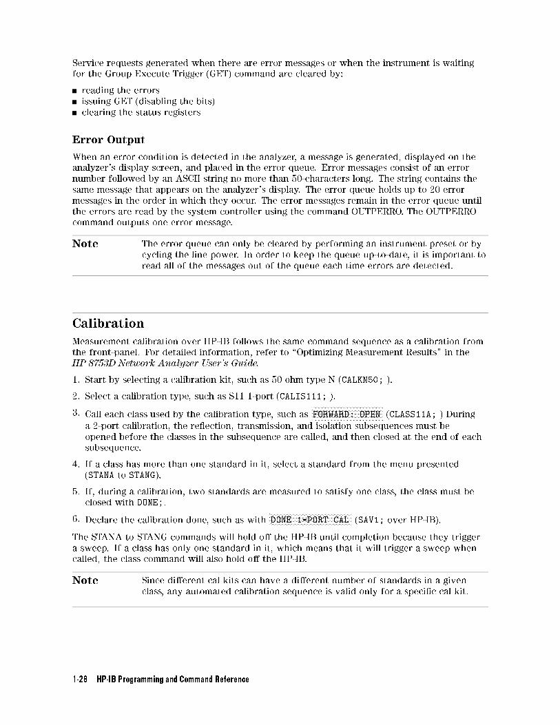
Service requests generated when there are error messages or when the instrument is waiting
for the Group Execute Trigger (GET) command are cleared by:
reading the errors
issuing GET (disabling the bits)
clearing the status registers
Error Output
When an error condition is detected in the analyzer, a message is generated, displayed on the
analyzer's display screen, and placed in the error queue. Error messages consist of an error
number followed by an ASCII string no more than 50-characters long. The string contains the
same message that appears on the analyzer's display. The error queue holds up to 20 error
messages in the order in which they occur. The error messages remain in the error queue until
the errors are read by the system controller using the command OUTPERRO. The OUTPERRO
command outputs one error message.
Note The error queue can only be cleared by performing an instrument preset or by
cycling the line power. In order to keep the queue up-to-date, it is important to
read all of the messages out of the queue each time errors are detected.
Calibration
Measurement calibration over HP-IB follows the same command sequence as a calibration from
the front-panel. For detailed information, refer to \Optimizing Measurement Results" in the
HP 8753D Network Analyzer User's Guide.
1. Start by selecting a calibration kit, such as 50 ohm type N (CALKN50; ).
2. Select a calibration type, such as S11 1-port (CALIS111; ).
3. Call each class used by the calibration type, such asNNNNNNNNNNNNNNNNNNNNNNNNNNNNNNNNNNNNNNNNNFORWARD: OPEN (CLASS11A; ) During
a 2-port calibration, the re ection, transmission, and isolation subsequences must be
opened before the classes in the subsequence are called, and then closed at the end of each
subsequence.
4. If a class has more than one standard in it, select a standard from the menu presented
(STANA to STANG).
5. If, during a calibration, two standards are measured to satisfy one class, the class must be
closed with DONE;.
6. Declare the calibration done, such as withNNNNNNNNNNNNNNNNNNNNNNNNNNNNNNNNNNNNNNNNNNNNNNNDONE 1-PORT CAL (SAV1; over HP-IB).
The STANA to STANG commands will hold o� the HP-IB until completion because they trigger
a sweep. If a class has only one standard in it, which means that it will trigger a sweep when
called, the class command will also hold o� the HP-IB.
Note Since di�erent cal kits can have a di�erent number of standards in a given
class, any automated calibration sequence is valid only for a speci�c cal kit.
1-28 HP-IB Programming and Command Reference
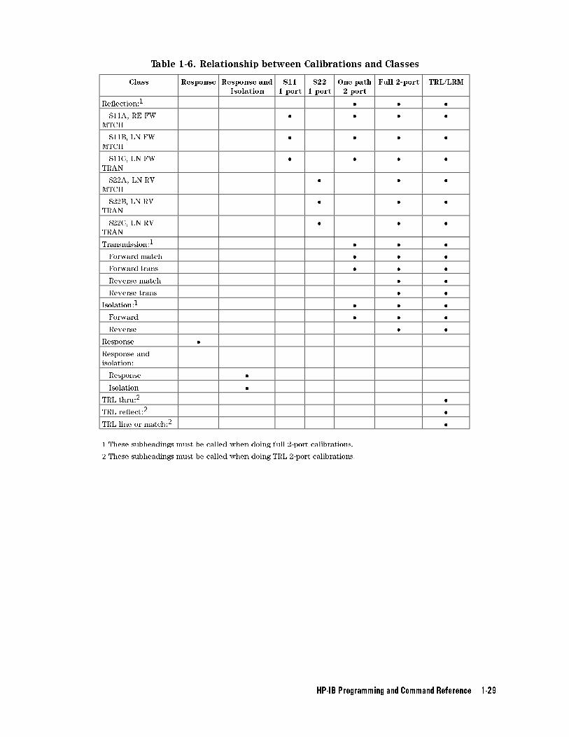
Table 1-6. Relationship between Calibrations and Classes
Class Response Response and
Isolation
S11
1-port
S22
1-port
One path
2-port
Full 2-port TRL/LRM
Re ection:1 � � �
S11A, RE FW
MTCH
� � � �
S11B, LN FW
MTCH
� � � �
S11C, LN FW
TRAN
� � � �
S22A, LN RV
MTCH
� � �
S22B, LN RV
TRAN
� � �
S22C, LN RV
TRAN
� � �
Transmission:1 � � �
Forward match � � �
Forward trans � � �
Reverse match � �
Reverse trans � �
Isolation:1 � � �
Forward � � �
Reverse � �
Response �
Response and
isolation:
Response �
Isolation �
TRL thru:2 �
TRL re ect:2 �
TRL line or match:2 �
1 These subheadings must be called when doing full 2-port calibrations.
2 These subheadings must be called when doing TRL 2-port calibrations.
HP-IB Programming and Command Reference 1-29
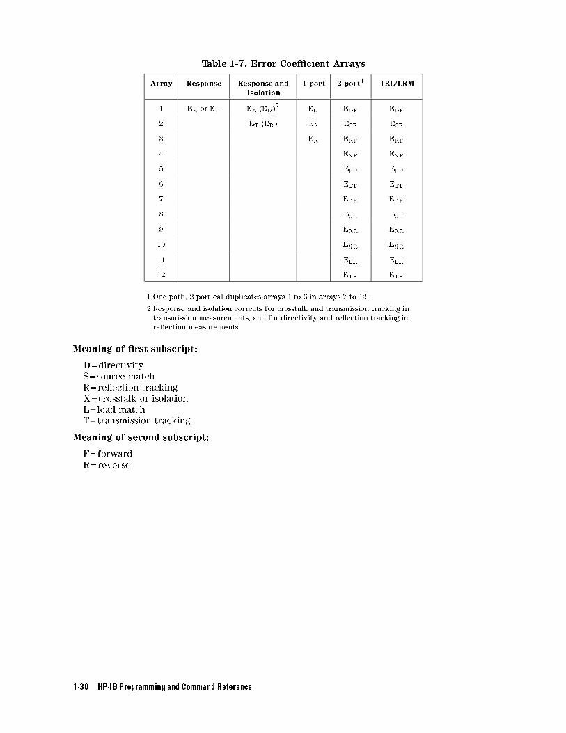
Table 1-7. Error Coe�cient Arrays
Array Response Response and
Isolation
1-port 2-port1 TRL/LRM
1 ER or ET EX (ED)2 ED EDF EDF
2 ET (ER) ES ESF ESF
3 ER ERF ERF
4 EXF EXF
5 ELF ELF
6 ETF ETF
7 EDR EDR
8 ESR ESR
9 ERR ERR
10 EXR EXR
11 ELR ELR
12 ETR ETR
1 One path, 2-port cal duplicates arrays 1 to 6 in arrays 7 to 12.
2 Response and isolation corrects for crosstalk and transmission tracking in
transmission measurements, and for directivity and re ection tracking in
re ection measurements.
Meaning of �rst subscript:
D=directivity
S=source match
R=re ection tracking
X=crosstalk or isolation
L=load match
T=transmission tracking
Meaning of second subscript:
F=forward
R=reverse
1-30 HP-IB Programming and Command Reference
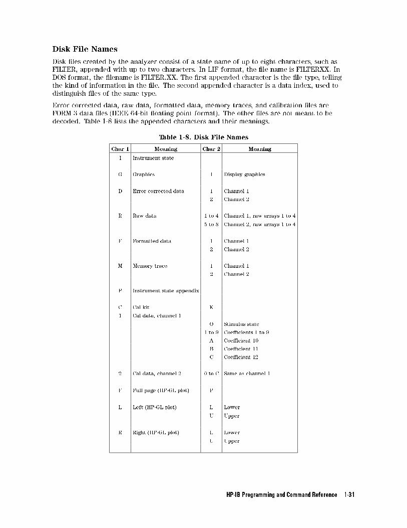
Disk File Names
Disk �les created by the analyzer consist of a state name of up to eight characters, such as
FILTER, appended with up to two characters. In LIF format, the �le name is FILTERXX. In
DOS format, the �lename is FILTER.XX. The �rst appended character is the �le type, telling
the kind of information in the �le. The second appended character is a data index, used to
distinguish �les of the same type.
Error corrected data, raw data, formatted data, memory traces, and calibration �les are
FORM 3 data �les (IEEE 64-bit oating point format). The other �les are not meant to be
decoded. Table 1-8 lists the appended characters and their meanings.
Table 1-8. Disk File Names
Char 1 Meaning Char 2 Meaning
I Instrument state
G Graphics 1 Display graphics
D Error corrected data 1 Channel 1
2 Channel 2
R Raw data 1 to 4 Channel 1, raw arrays 1 to 4
5 to 8 Channel 2, raw arrays 1 to 4
F Formatted data 1 Channel 1
2 Channel 2
M Memory trace 1 Channel 1
2 Channel 2
P Instrument state appendix
C Cal kit K
1 Cal data, channel 1
O Stimulus state
1 to 9 Coe�cients 1 to 9
A Coe�cient 10
B Coe�cient 11
C Coe�cient 12
2 Cal data, channel 2 0 to C Same as channel 1
F Full page (HP-GL plot) P
L Left (HP-GL plot) L Lower
U Upper
R Right (HP-GL plot) L Lower
U Upper
HP-IB Programming and Command Reference 1-31
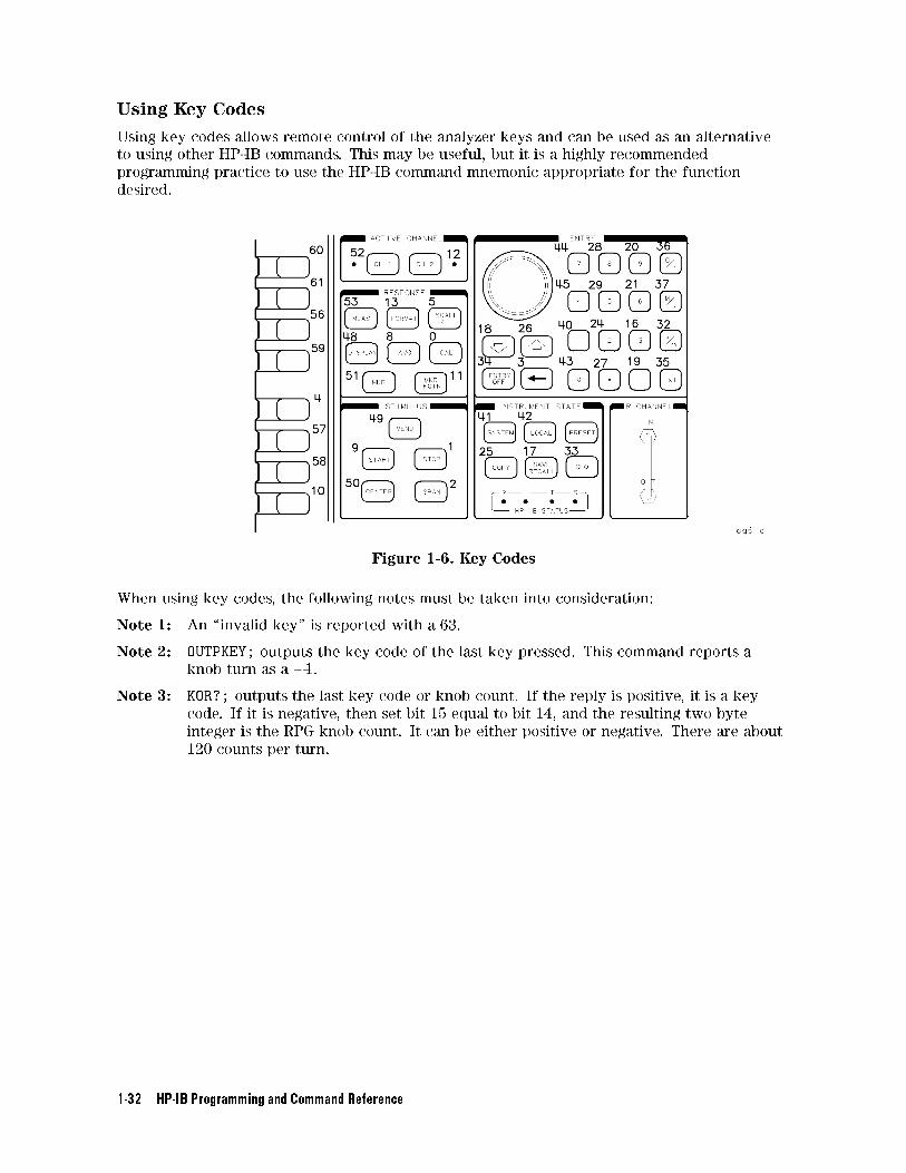
Using Key Codes
Using key codes allows remote control of the analyzer keys and can be used as an alternative
to using other HP-IB commands. This may be useful, but it is a highly recommended
programming practice to use the HP-IB command mnemonic appropriate for the function
desired.
Figure 1-6. Key Codes
When using key codes, the following notes must be taken into consideration:
Note 1: An \invalid key" is reported with a 63.
Note 2: OUTPKEY; outputs the key code of the last key pressed. This command reports a
knob turn as a �1.
Note 3: KOR?; outputs the last key code or knob count. If the reply is positive, it is a key
code. If it is negative, then set bit 15 equal to bit 14, and the resulting two byte
integer is the RPG knob count. It can be either positive or negative. There are about
120 counts per turn.
1-32 HP-IB Programming and Command Reference
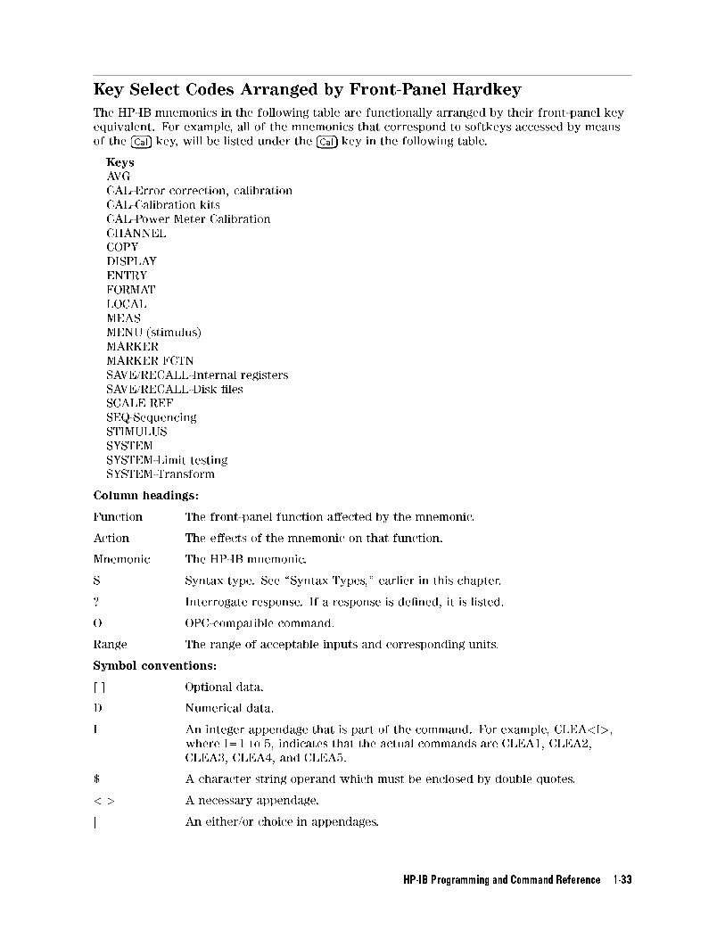
Key Select Codes Arranged by Front-Panel Hardkey
The HP-IB mnemonics in the following table are functionally arranged by their front-panel key
equivalent. For example, all of the mnemonics that correspond to softkeys accessed by means
of the �Cal� key, will be listed under the �Cal� key in the following table.
KeysAVG
CAL-Error correction, calibration
CAL-Calibration kits
CAL-Power Meter Calibration
CHANNEL
COPY
DISPLAY
ENTRY
FORMAT
LOCAL
MEAS
MENU (stimulus)
MARKER
MARKER FCTN
SAVE/RECALL-Internal registers
SAVE/RECALL-Disk �les
SCALE REF
SEQ-Sequencing
STIMULUS
SYSTEM
SYSTEM-Limit testing
SYSTEM-Transform
Column headings:
Function The front-panel function a�ected by the mnemonic.
Action The e�ects of the mnemonic on that function.
Mnemonic The HP-IB mnemonic.
S Syntax type. See \Syntax Types," earlier in this chapter.
? Interrogate response. If a response is de�ned, it is listed.
O OPC-compatible command.
Range The range of acceptable inputs and corresponding units.
Symbol conventions:
[ ] Optional data.
D Numerical data.
I An integer appendage that is part of the command. For example, CLEA<I>,
where I=1 to 5, indicates that the actual commands are CLEA1, CLEA2,
CLEA3, CLEA4, and CLEA5.
$ A character string operand which must be enclosed by double quotes.
< > A necessary appendage.
j An either/or choice in appendages.
HP-IB Programming and Command Reference 1-33
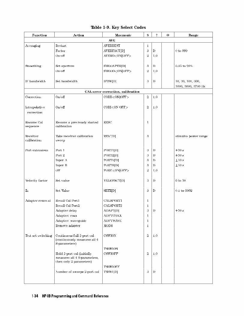
Table 1-9. Key Select Codes
Function Action Mnemonic S ? O Range
AVG
Averaging Restart AVERREST 1
Factor AVERFACT[D] 3 D 0 to 999
On/o� AVERO<ONjOFF> 2 1,0
Smoothing Set aperture SMOOAPER[D] 3 D 0.05 to 20%
On/o� SMOOO<ONjOFF> 2 1,0
IF bandwidth Set bandwidth IFBW[D] 3 D 10, 30, 100, 300,
1000, 3000, 3700 Hz
CAL-error correction, calibration
Correction On/o� CORR<ONjOFF> 2 1,0
Interpolative On/o� CORI<ONjOFF> 2 1,0
correction
Resume Cal
sequence
Resume a previously started
calibration
RESC 1
Receiver
calibration
Take receiver calibration
sweep
REIC[D] 3 stimulus power range
Port extensions Port 1 PORT1[D] 3 D �10 s
Port 2 PORT2[D] 3 D �10 s
Input A PORTA[D] 3 D �10 s
Input B PORTB[D] 3 D �10 s
O� PORE<ONjOFF> 2 1,0
Velocity factor Set value VELOFACT[D] 3 D 0 to 10
Z0 Set Value SETZ[D] 3 D 0.1 to 500
Adapter removal Recall Cal Port1 CALSPORT1 1
Recall Cal Port2 CALSPORT2 1
Adapter delay ADAP1[D] 3 D �10 s
Adapter: coax ADPTCOAX 1
Adapter: waveguide ADPTWAVE 1
Remove adapter MODS 1
Test set switching Continuous/full 2-port cal
(continuously measures all 4
S-parameters)
CSWION 2 1,0
TSSWION
Hold 2-port cal (initially
measures all 4 S-parameters,
then only 2 parameters)
CSWIOFF 2 1,0
TSSWIOFF
Number of sweeps 2-port cal TSSWI[D] 3 D
1-34 HP-IB Programming and Command Reference
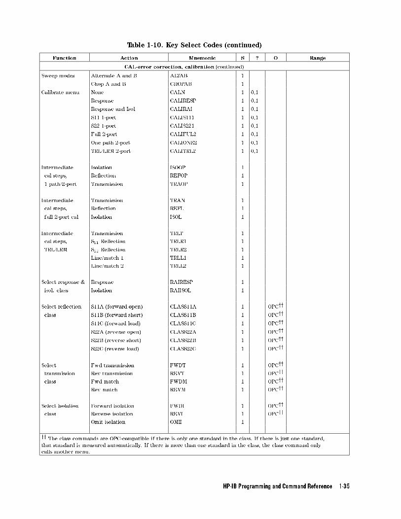
Table 1-10. Key Select Codes (continued)
Function Action Mnemonic S ? O Range
CAL-error correction, calibration (continued)
Sweep modes Alternate A and B ALTAB 1
Chop A and B CHOPAB 1
Calibrate menu None CALN 1 0,1
Response CALIRESP 1 0,1
Response and Isol CALIRAI 1 0,1
S11 1-port CALIS111 1 0,1
S22 1-port CALIS221 1 0,1
Full 2-port CALIFUL2 1 0,1
One path 2-port CALIONE2 1 0,1
TRL/LRM 2-port CALITRL2 1 0,1
Intermediate Isolation ISOOP 1
cal steps, Re ection REFOP 1
1 path/2-port Transmission TRAOP 1
Intermediate Transmission TRAN 1
cal steps, Re ection REFL 1
full 2-port cal Isolation ISOL 1
Intermediate Transmission TRLT 1
cal steps, S11 Re ection TRLR1 1
TRL/LRM S22 Re ection TRLR2 1
Line/match 1 TRLL1 1
Line/match 2 TRLL2 1
Select response & Response RAIRESP 1
isol. class Isolation RAIISOL 1
Select re ection S11A (forward open) CLASS11A 1 OPCyy
class S11B (forward short) CLASS11B 1 OPCyy
S11C (forward load) CLASS11C 1 OPCyy
S22A (reverse open) CLASS22A 1 OPCyy
S22B (reverse short) CLASS22B 1 OPCyy
S22C (reverse load) CLASS22C 1 OPCyy
Select Fwd transmission FWDT 1 OPCyy
transmission Rev transmission REVT 1 OPCyy
class Fwd match FWDM 1 OPCyy
Rev match REVM 1 OPCyy
Select isolation Forward isolation FWDI 1 OPCyy
class Reverse isolation REVI 1 OPCyy
Omit isolation OMII 1
yy The class commands are OPC-compatible if there is only one standard in the class. If there is just one standard,
that standard is measured automatically. If there is more than one standard in the class, the class command only
calls another menu.
HP-IB Programming and Command Reference 1-35
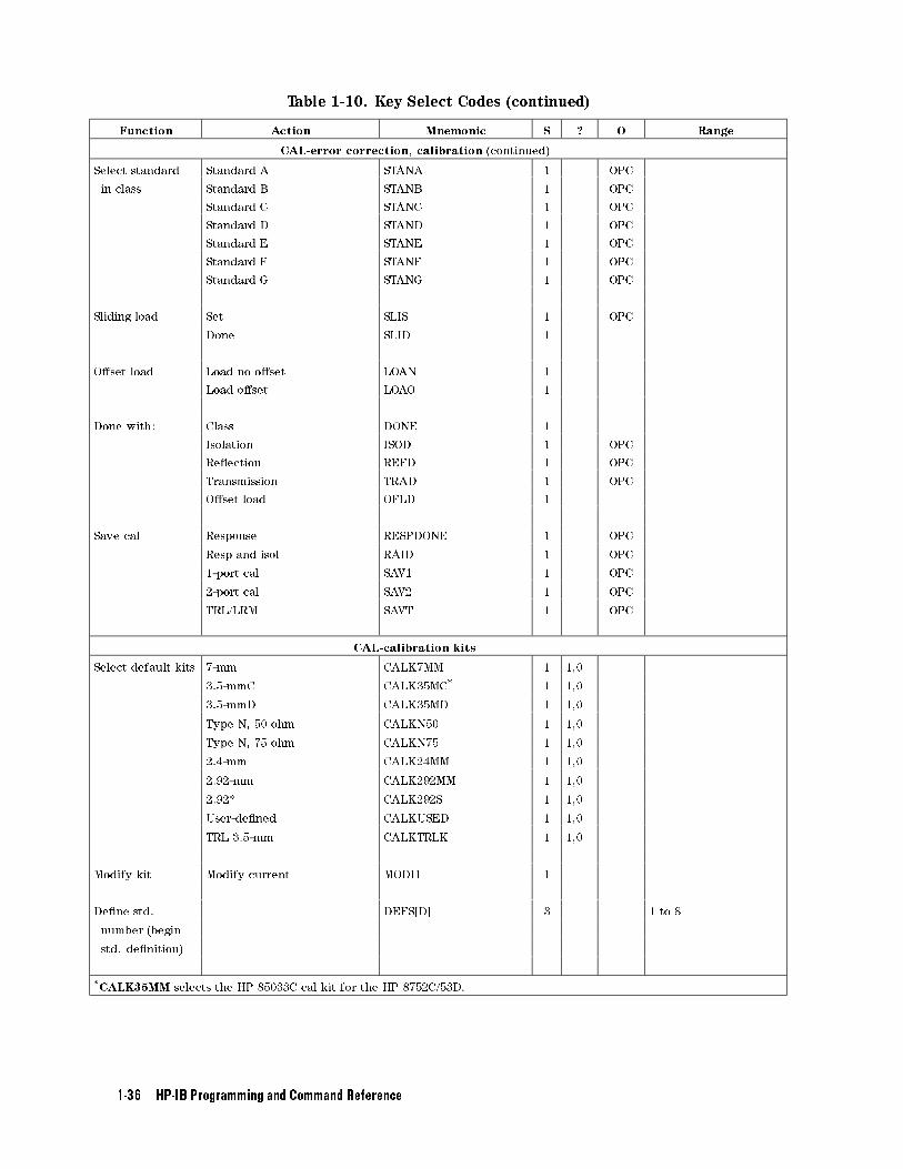
Table 1-10. Key Select Codes (continued)
Function Action Mnemonic S ? O Range
CAL-error correction, calibration (continued)
Select standard Standard A STANA 1 OPC
in class Standard B STANB 1 OPC
Standard C STANC 1 OPC
Standard D STAND 1 OPC
Standard E STANE 1 OPC
Standard F STANF 1 OPC
Standard G STANG 1 OPC
Sliding load Set SLIS 1 OPC
Done SLID 1
O�set load Load no o�set LOAN 1
Load o�set LOAO 1
Done with: Class DONE 1
Isolation ISOD 1 OPC
Re ection REFD 1 OPC
Transmission TRAD 1 OPC
O�set load OFLD 1
Save cal Response RESPDONE 1 OPC
Resp and isol RAID 1 OPC
1-port cal SAV1 1 OPC
2-port cal SAV2 1 OPC
TRL/LRM SAVT 1 OPC
CAL-calibration kits
Select default kits 7-mm CALK7MM 1 1,0
3.5-mmC CALK35MC* 1 1,0
3.5-mmD CALK35MD 1 1,0
Type N, 50 ohm CALKN50 1 1,0
Type N, 75 ohm CALKN75 1 1,0
2.4-mm CALK24MM 1 1,0
2.92-mm CALK292MM 1 1,0
2.92* CALK292S 1 1,0
User-de�ned CALKUSED 1 1,0
TRL 3.5-mm CALKTRLK 1 1,0
Modify kit Modify current MODI1 1
De�ne std. DEFS[D] 3 1 to 8
number (begin
std. de�nition)
*CALK35MM selects the HP 85033C cal kit for the HP 8752C/53D.
1-36 HP-IB Programming and Command Reference
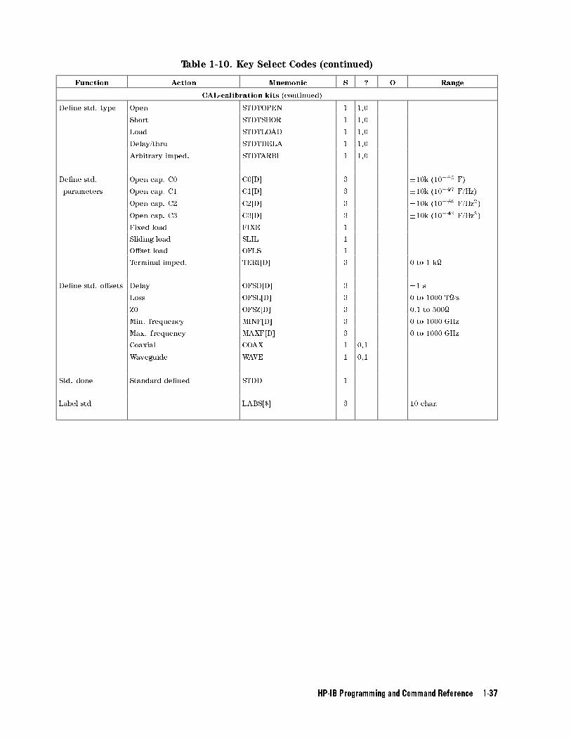
Table 1-10. Key Select Codes (continued)
Function Action Mnemonic S ? O Range
CAL-calibration kits (continued)
De�ne std. type Open STDTOPEN 1 1,0
Short STDTSHOR 1 1,0
Load STDTLOAD 1 1,0
Delay/thru STDTDELA 1 1,0
Arbitrary imped. STDTARBI 1 1,0
De�ne std. Open cap. C0 C0[D] 3 �10k (10�15 F)
parameters Open cap. C1 C1[D] 3 �10k (10�27 F/Hz)
Open cap. C2 C2[D] 3 �10k (10�36 F/Hz2)
Open cap. C3 C3[D] 3 �10k (10�45 F/Hz3)
Fixed load FIXE 1
Sliding load SLIL 1
O�set load OFLS 1
Terminal imped. TERI[D] 3 0 to 1 k
De�ne std. o�sets Delay OFSD[D] 3 �1 s
Loss OFSL[D] 3 0 to 1000 T/s
Z0 OFSZ[D] 3 0.1 to 500
Min. frequency MINF[D] 3 0 to 1000 GHz
Max. frequency MAXF[D] 3 0 to 1000 GHz
Coaxial COAX 1 0,1
Waveguide WAVE 1 0,1
Std. done Standard de�ned STDD 1
Label std LABS[$] 3 10 char.
HP-IB Programming and Command Reference 1-37
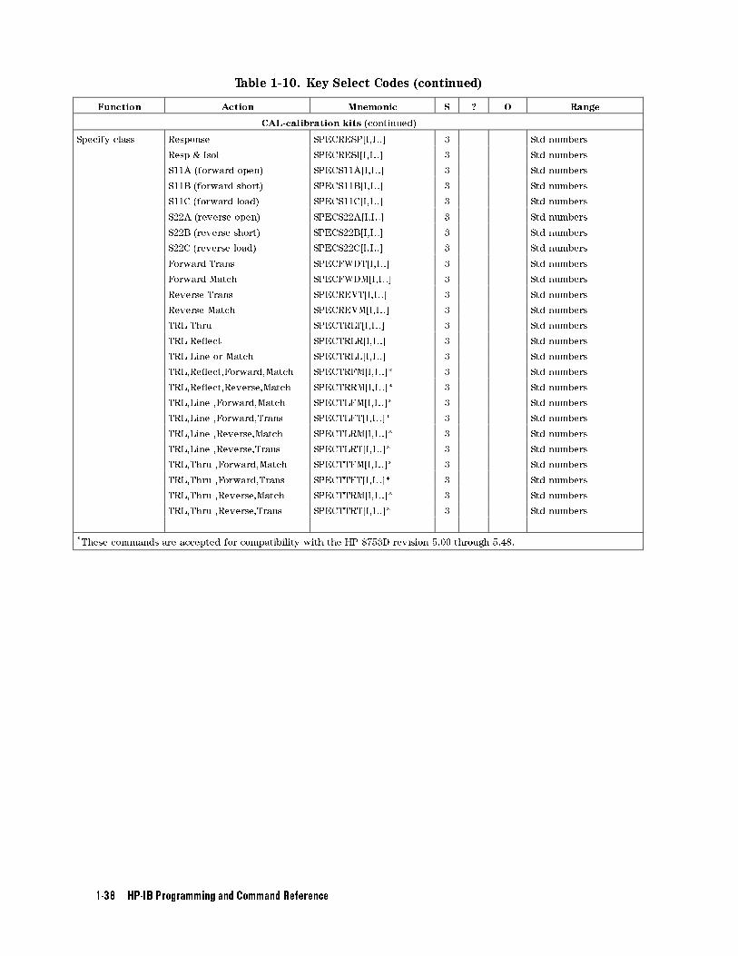
Table 1-10. Key Select Codes (continued)
Function Action Mnemonic S ? O Range
CAL-calibration kits (continued)
Specify class Response SPECRESP[I,I..] 3 Std numbers
Resp & Isol SPECRESI[I,I..] 3 Std numbers
S11A (forward open) SPECS11A[I,I..] 3 Std numbers
S11B (forward short) SPECS11B[I,I..] 3 Std numbers
S11C (forward load) SPECS11C[I,I..] 3 Std numbers
S22A (reverse open) SPECS22A[I,I..] 3 Std numbers
S22B (reverse short) SPECS22B[I,I..] 3 Std numbers
S22C (reverse load) SPECS22C[I,I..] 3 Std numbers
Forward Trans SPECFWDT[I,I..] 3 Std numbers
Forward Match SPECFWDM[I,I..] 3 Std numbers
Reverse Trans SPECREVT[I,I..] 3 Std numbers
Reverse Match SPECREVM[I,I..] 3 Std numbers
TRL Thru SPECTRLT[I,I..] 3 Std numbers
TRL Re ect SPECTRLR[I,I..] 3 Std numbers
TRL Line or Match SPECTRLL[I,I..] 3 Std numbers
TRL,Re ect,Forward,Match SPECTRFM[I,I..]* 3 Std numbers
TRL,Re ect,Reverse,Match SPECTRRM[I,I..]* 3 Std numbers
TRL,Line ,Forward,Match SPECTLFM[I,I..]* 3 Std numbers
TRL,Line ,Forward,Trans SPECTLFT[I,I..]* 3 Std numbers
TRL,Line ,Reverse,Match SPECTLRM[I,I..]* 3 Std numbers
TRL,Line ,Reverse,Trans SPECTLRT[I,I..]* 3 Std numbers
TRL,Thru ,Forward,Match SPECTTFM[I,I..]* 3 Std numbers
TRL,Thru ,Forward,Trans SPECTTFT[I,I..]* 3 Std numbers
TRL,Thru ,Reverse,Match SPECTTRM[I,I..]* 3 Std numbers
TRL,Thru ,Reverse,Trans SPECTTRT[I,I..]* 3 Std numbers
*These commands are accepted for compatibility with the HP 8753D revision 5.00 through 5.48.
1-38 HP-IB Programming and Command Reference
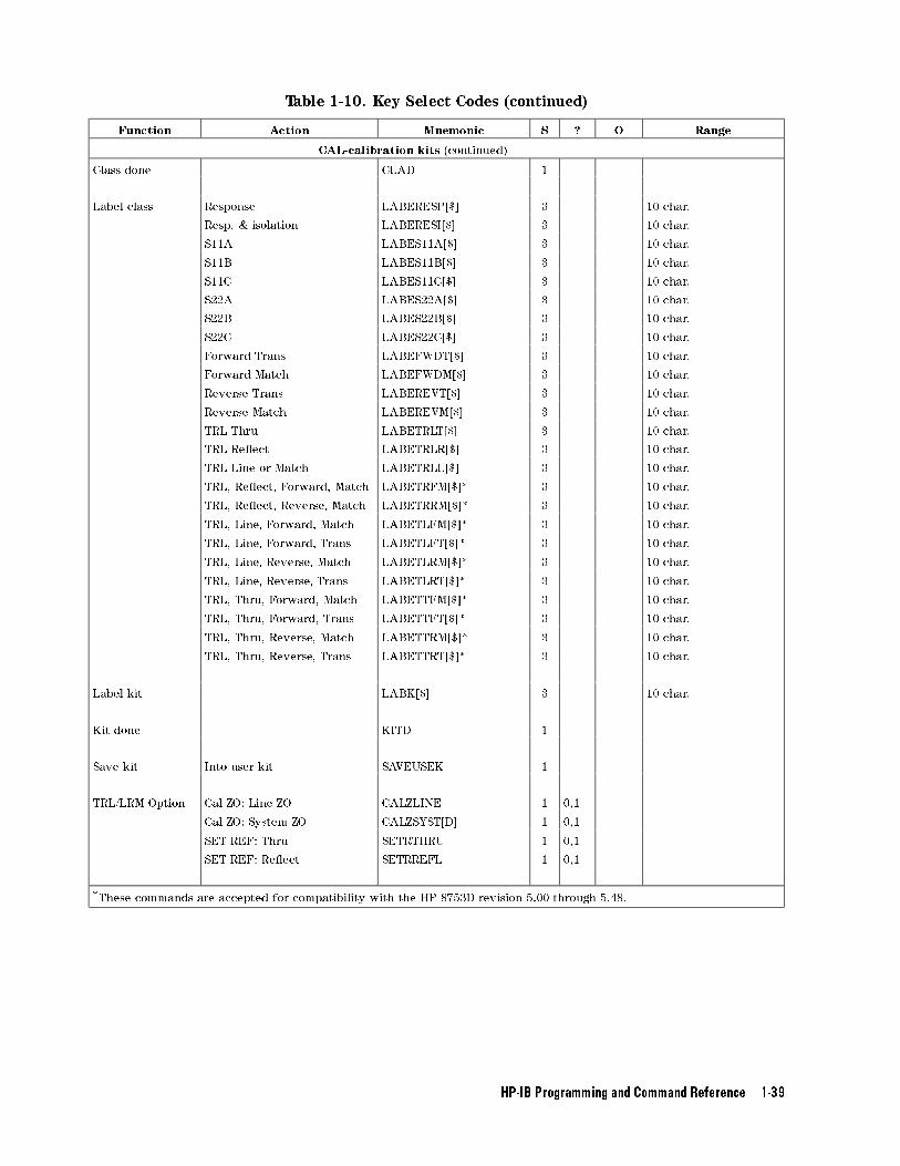
Table 1-10. Key Select Codes (continued)
Function Action Mnemonic S ? O Range
CAL-calibration kits (continued)
Class done CLAD 1
Label class Response LABERESP[$] 3 10 char.
Resp. & isolation LABERESI[$] 3 10 char.
S11A LABES11A[$] 3 10 char.
S11B LABES11B[$] 3 10 char.
S11C LABES11C[$] 3 10 char.
S22A LABES22A[$] 3 10 char.
S22B LABES22B[$] 3 10 char.
S22C LABES22C[$] 3 10 char.
Forward Trans LABEFWDT[$] 3 10 char.
Forward Match LABEFWDM[$] 3 10 char.
Reverse Trans LABEREVT[$] 3 10 char.
Reverse Match LABEREVM[$] 3 10 char.
TRL Thru LABETRLT[$] 3 10 char.
TRL Re ect LABETRLR[$] 3 10 char.
TRL Line or Match LABETRLL[$] 3 10 char.
TRL, Re ect, Forward, Match LABETRFM[$]* 3 10 char.
TRL, Re ect, Reverse, Match LABETRRM[$]* 3 10 char.
TRL, Line, Forward, Match LABETLFM[$]* 3 10 char.
TRL, Line, Forward, Trans LABETLFT[$]* 3 10 char.
TRL, Line, Reverse, Match LABETLRM[$]* 3 10 char.
TRL, Line, Reverse, Trans LABETLRT[$]* 3 10 char.
TRL, Thru, Forward, Match LABETTFM[$]* 3 10 char.
TRL, Thru, Forward, Trans LABETTFT[$]* 3 10 char.
TRL, Thru, Reverse, Match LABETTRM[$]* 3 10 char.
TRL, Thru, Reverse, Trans LABETTRT[$]* 3 10 char.
Label kit LABK[$] 3 10 char.
Kit done KITD 1
Save kit Into user kit SAVEUSEK 1
TRL/LRM Option Cal ZO: Line ZO CALZLINE 1 0,1
Cal ZO: System ZO CALZSYST[D] 1 0,1
SET REF: Thru SETRTHRU 1 0,1
SET REF: Re ect SETRREFL 1 0,1
*These commands are accepted for compatibility with the HP 8753D revision 5.00 through 5.48.
HP-IB Programming and Command Reference 1-39
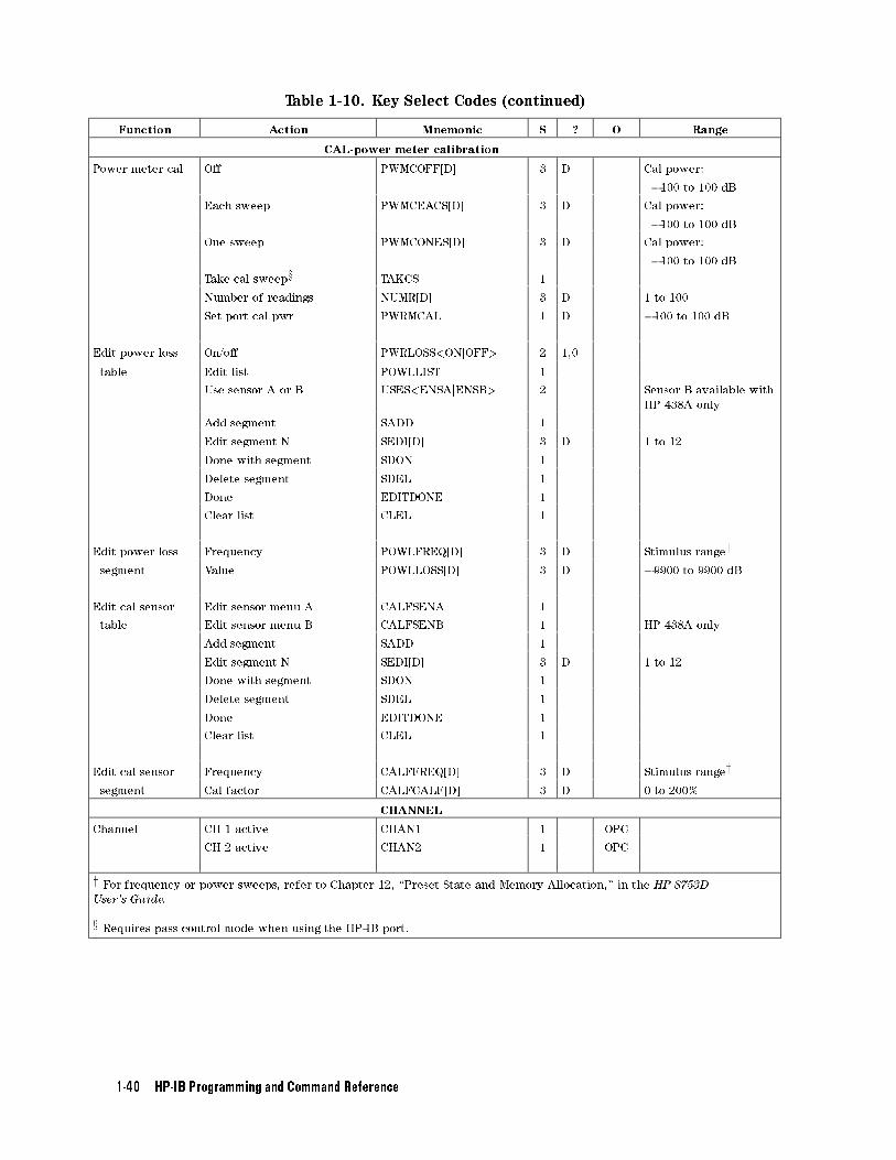
Table 1-10. Key Select Codes (continued)
Function Action Mnemonic S ? O Range
CAL-power meter calibration
Power meter cal O� PWMCOFF[D] 3 D Cal power:
�100 to 100 dB
Each sweep PWMCEACS[D] 3 D Cal power:
�100 to 100 dB
One sweep PWMCONES[D] 3 D Cal power:
�100 to 100 dB
Take cal sweepx TAKCS 1
Number of readings NUMR[D] 3 D 1 to 100
Set port cal pwr PWRMCAL 1 D �100 to 100 dB
Edit power loss On/o� PWRLOSS<ONjOFF> 2 1,0
table Edit list POWLLIST 1
Use sensor A or B USES<ENSAjENSB> 2 Sensor B available with
HP 438A only
Add segment SADD 1
Edit segment N SEDI[D] 3 D 1 to 12
Done with segment SDON 1
Delete segment SDEL 1
Done EDITDONE 1
Clear list CLEL 1
Edit power loss Frequency POWLFREQ[D] 3 D Stimulus rangey
segment Value POWLLOSS[D] 3 D �9900 to 9900 dB
Edit cal sensor Edit sensor menu A CALFSENA 1
table Edit sensor menu B CALFSENB 1 HP 438A only
Add segment SADD 1
Edit segment N SEDI[D] 3 D 1 to 12
Done with segment SDON 1
Delete segment SDEL 1
Done EDITDONE 1
Clear list CLEL 1
Edit cal sensor Frequency CALFFREQ[D] 3 D Stimulus rangey
segment Cal factor CALFCALF[D] 3 D 0 to 200%
CHANNEL
Channel CH 1 active CHAN1 1 OPC
CH 2 active CHAN2 1 OPC
y For frequency or power sweeps, refer to Chapter 12, \Preset State and Memory Allocation," in the HP 8753D
User's Guide.
x Requires pass control mode when using the HP-IB port.
1-40 HP-IB Programming and Command Reference
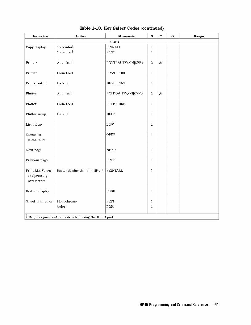
Table 1-10. Key Select Codes (continued)
Function Action Mnemonic S ? O Range
COPY
Copy display To printerx PRINALL 1
To plotterx PLOT 1
Printer Auto feed PRNTRAUTF<ONjOFF> 2 1,0
Printer Form feed PRNTRFORF 1
Printer setup Default DEFLPRINT 1
Plotter Auto feed PLTTRAUTF<ONjOFF> 2 1,0
Plotter Form feed PLTTRFORF 1
Plotter setup Default DFLT 1
List values LISV 1
Operating OPEP 1
parameters
Next page NEXP 1
Previous page PREP 1
Print List Values Raster display dump to HP-IBx PRINTALL 1
or Operating
parameters
Restore display RESD 1
Select print color Monochrome PRIS 1
Color PRIC 1
x Requires pass control mode when using the HP-IB port.
HP-IB Programming and Command Reference 1-41
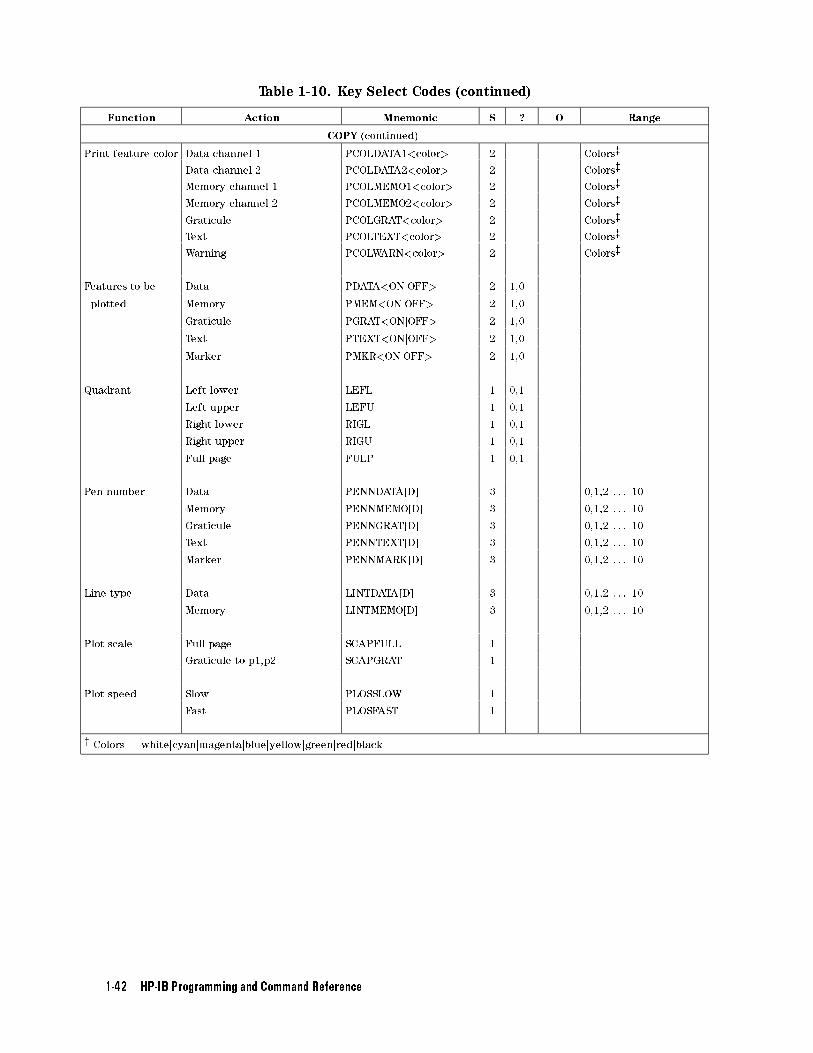
Table 1-10. Key Select Codes (continued)
Function Action Mnemonic S ? O Range
COPY (continued)
Print feature color Data channel 1 PCOLDATA1<color> 2 Colorsz
Data channel 2 PCOLDATA2<color> 2 Colorsz
Memory channel 1 PCOLMEMO1<color> 2 Colorsz
Memory channel 2 PCOLMEMO2<color> 2 Colorsz
Graticule PCOLGRAT<color> 2 Colorsz
Text PCOLTEXT<color> 2 Colorsz
Warning PCOLWARN<color> 2 Colorsz
Features to be Data PDATA<ONjOFF> 2 1,0
plotted Memory PMEM<ONjOFF> 2 1,0
Graticule PGRAT<ONjOFF> 2 1,0
Text PTEXT<ONjOFF> 2 1,0
Marker PMKR<ONjOFF> 2 1,0
Quadrant Left lower LEFL 1 0,1
Left upper LEFU 1 0,1
Right lower RIGL 1 0,1
Right upper RIGU 1 0,1
Full page FULP 1 0,1
Pen number Data PENNDATA[D] 3 0,1,2 . . . 10
Memory PENNMEMO[D] 3 0,1,2 . . . 10
Graticule PENNGRAT[D] 3 0,1,2 . . . 10
Text PENNTEXT[D] 3 0,1,2 . . . 10
Marker PENNMARK[D] 3 0,1,2 . . . 10
Line type Data LINTDATA[D] 3 0,1,2 . . . 10
Memory LINTMEMO[D] 3 0,1,2 . . . 10
Plot scale Full page SCAPFULL 1
Graticule to p1,p2 SCAPGRAT 1
Plot speed Slow PLOSSLOW 1
Fast PLOSFAST 1
z Colors = whitejcyanjmagentajbluejyellowjgreenjredjblack
1-42 HP-IB Programming and Command Reference
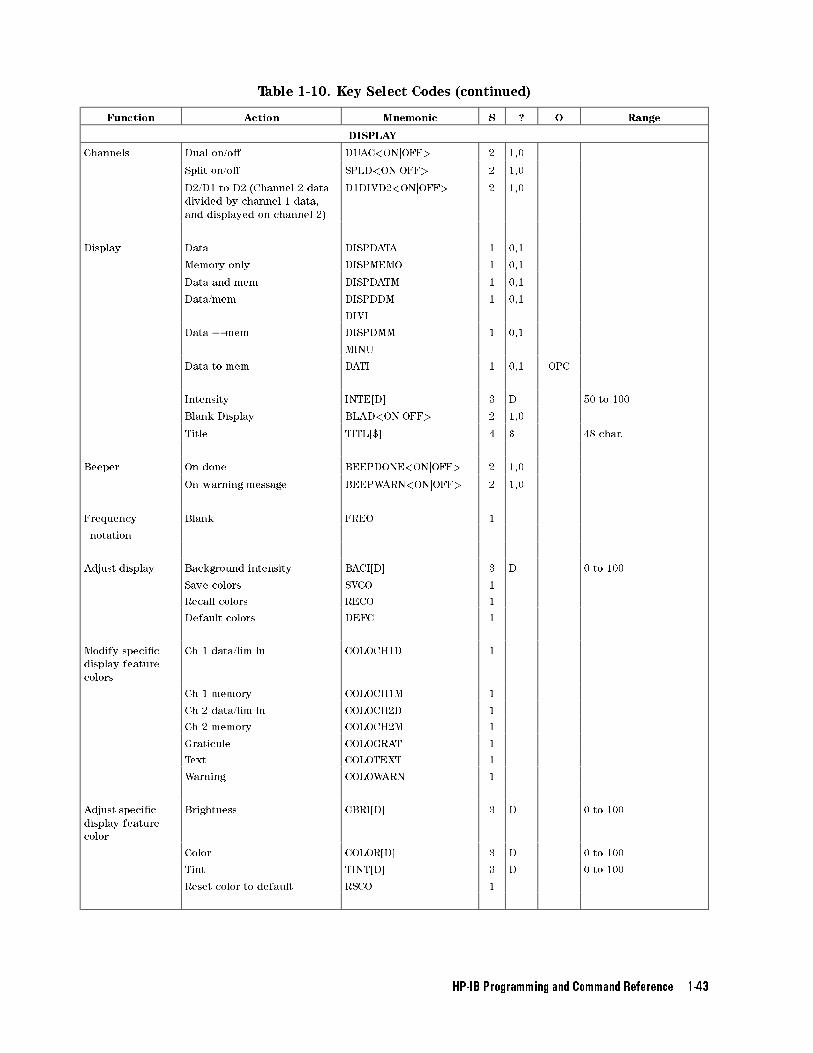
Table 1-10. Key Select Codes (continued)
Function Action Mnemonic S ? O Range
DISPLAY
Channels Dual on/o� DUAC<ONjOFF> 2 1,0
Split on/o� SPLD<ONjOFF> 2 1,0
D2/D1 to D2 (Channel 2 data
divided by channel 1 data,
and displayed on channel 2)
D1DIVD2<ONjOFF> 2 1,0
Display Data DISPDATA 1 0,1
Memory only DISPMEMO 1 0,1
Data and mem DISPDATM 1 0,1
Data/mem DISPDDM 1 0,1
DIVI
Data | mem DISPDMM 1 0,1
MINU
Data to mem DATI 1 0,1 OPC
Intensity INTE[D] 3 D 50 to 100
Blank Display BLAD<ONjOFF> 2 1,0
Title TITL[$] 4 $ 48 char.
Beeper On done BEEPDONE<ONjOFF> 2 1,0
On warning message BEEPWARN<ONjOFF> 2 1,0
Frequency Blank FREO 1
notation
Adjust display Background intensity BACI[D] 3 D 0 to 100
Save colors SVCO 1
Recall colors RECO 1
Default colors DEFC 1
Modify speci�c
display feature
colors
Ch 1 data/lim ln COLOCH1D 1
Ch 1 memory COLOCH1M 1
Ch 2 data/lim ln COLOCH2D 1
Ch 2 memory COLOCH2M 1
Graticule COLOGRAT 1
Text COLOTEXT 1
Warning COLOWARN 1
Adjust speci�c
display feature
color
Brightness CBRI[D] 3 D 0 to 100
Color COLOR[D] 3 D 0 to 100
Tint TINT[D] 3 D 0 to 100
Reset color to default RSCO 1
HP-IB Programming and Command Reference 1-43
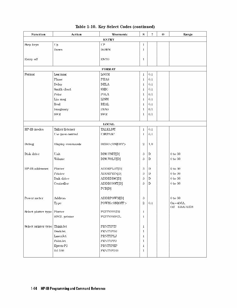
Table 1-10. Key Select Codes (continued)
Function Action Mnemonic S ? O Range
ENTRY
Step keys Up UP 1
Down DOWN 1
Entry o� ENTO 1
FORMAT
Format Log mag LOGM 1 0,1
Phase PHAS 1 0,1
Delay DELA 1 0,1
Smith chart SMIC 1 0,1
Polar POLA 1 0,1
Lin mag LINM 1 0,1
Real REAL 1 0,1
Imaginary IMAG 1 0,1
SWR SWR 1 0,1
LOCAL
HP-IB modes Talker/listener TALKLIST 1 0,1
Use pass control USEPASC 1 0,1
Debug Display commands DEBU<ONjOFF> 2 1,0
Disk drive Unit DISCUNIT[D] 3 D 0 to 30
Volume DISCVOLU[D] 3 D 0 to 30
HP-IB addresses Plotter ADDRPLOT[D] 3 D 0 to 30
Printer ADDRPRIN[D] 3 D 0 to 30
Disk drive ADDRDISC[D] 3 D 0 to 30
Controller ADDRCONT[D] 3 D 0 to 30
PCB[D]
Power meter Address ADDRPOWM[D] 3 0 to 30
Type POWM<ONjOFF> 2 0,1 On=436A,
O�=438A/437B
Select plotter type Plotter PLTTYPPLTR 1
HPGL printer PLTTYPHPGL 1
Select printer type ThinkJet PRNTYPTJ 1
DeskJet PRNTYPDJ 1
LaserJet PRNTYPLJ 1
PaintJet PRNTYPPJ 1
Epson-P2 PRNTYPEP 1
DJ 540 PRNTYP540 1
1-44 HP-IB Programming and Command Reference
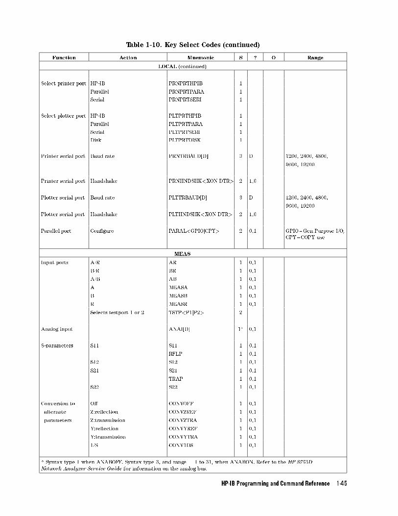
Table 1-10. Key Select Codes (continued)
Function Action Mnemonic S ? O Range
LOCAL (continued)
Select printer port HP-IB PRNPRTHPIB 1
Parallel PRNPRTPARA 1
Serial PRNPRTSERI 1
Select plotter port HP-IB PLTPRTHPIB 1
Parallel PLTPRTPARA 1
Serial PLTPRTSERI 1
Disk PLTPRTDISK 1
Printer serial port Baud rate PRNTRBAUD[D] 3 D 1200, 2400, 4800,
9600, 19200
Printer serial port Handshake PRNHNDSHK<XONjDTR> 2 1,0
Plotter serial port Baud rate PLTTRBAUD[D] 3 D 1200, 2400, 4800,
9600, 19200
Plotter serial port Handshake PLTHNDSHK<XONjDTR> 2 1,0
Parallel port Con�gure PARAL<GPIOjCPY> 2 0,1 GPIO=Gen.Purpose I/O,
CPY=COPY use
MEAS
Input ports A/R AR 1 0,1
B/R BR 1 0,1
A/B AB 1 0,1
A MEASA 1 0,1
B MEASB 1 0,1
R MEASR 1 0,1
Selects testport 1 or 2 TSTP<P1jP2> 2
Analog input ANAI[D] 1* 0,1
S-parameters S11 S11 1 0,1
RFLP 1 0,1
S12 S12 1 0,1
S21 S21 1 0,1
TRAP 1 0,1
S22 S22 1 0,1
Conversion to O� CONVOFF 1 0,1
alternate Z:re ection CONVZREF 1 0,1
parameters Z:transmission CONVZTRA 1 0,1
Y:re ection CONVYREF 1 0,1
Y:transmission CONVYTRA 1 0,1
1/S CONV1DS 1 0,1
* Syntax type 1 when ANABOFF. Syntax type 3, and range = 1 to 31, when ANABON. Refer to the HP 8753D
Network Analyzer Service Guide for information on the analog bus.
HP-IB Programming and Command Reference 1-45
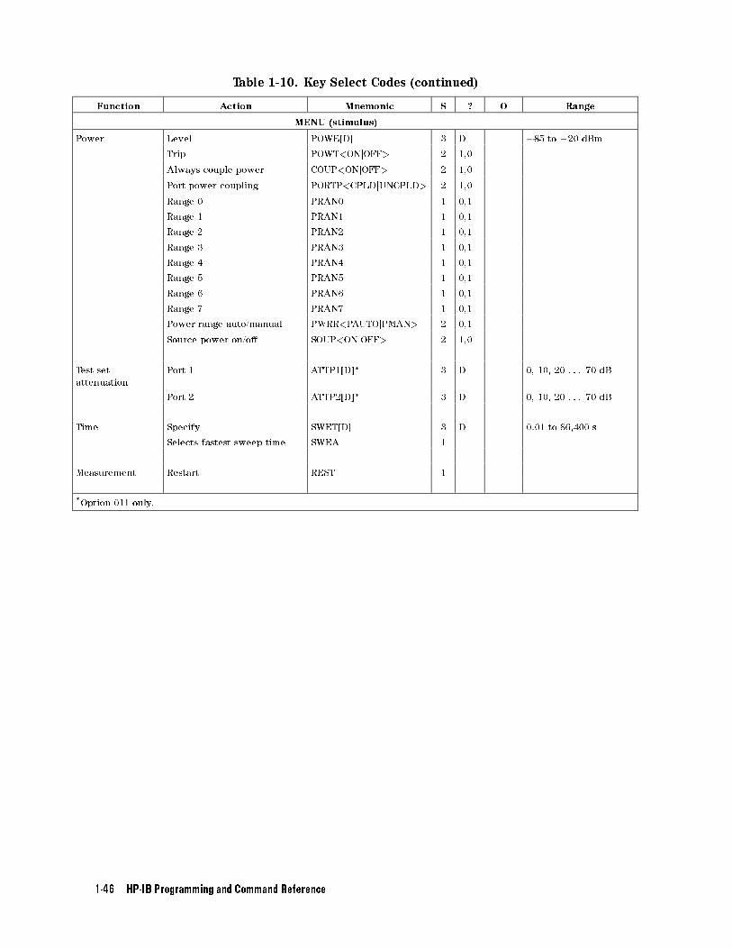
Table 1-10. Key Select Codes (continued)
Function Action Mnemonic S ? O Range
MENU (stimulus)
Power Level POWE[D] 3 D �85 to +20 dBm
Trip POWT<ONjOFF> 2 1,0
Always couple power COUP<ONjOFF> 2 1,0
Port power coupling PORTP<CPLDjUNCPLD> 2 1,0
Range 0 PRAN0 1 0,1
Range 1 PRAN1 1 0,1
Range 2 PRAN2 1 0,1
Range 3 PRAN3 1 0,1
Range 4 PRAN4 1 0,1
Range 5 PRAN5 1 0,1
Range 6 PRAN6 1 0,1
Range 7 PRAN7 1 0,1
Power range auto/manual PWRR<PAUTOjPMAN> 2 0,1
Source power on/o� SOUP<ONjOFF> 2 1,0
Test set
attenuation
Port 1 ATTP1[D]* 3 D 0, 10, 20 . . . 70 dB
Port 2 ATTP2[D]* 3 D 0, 10, 20 . . . 70 dB
Time Specify SWET[D] 3 D 0.01 to 86,400 s
Selects fastest sweep time SWEA 1
Measurement Restart REST 1
*Option 011 only.
1-46 HP-IB Programming and Command Reference
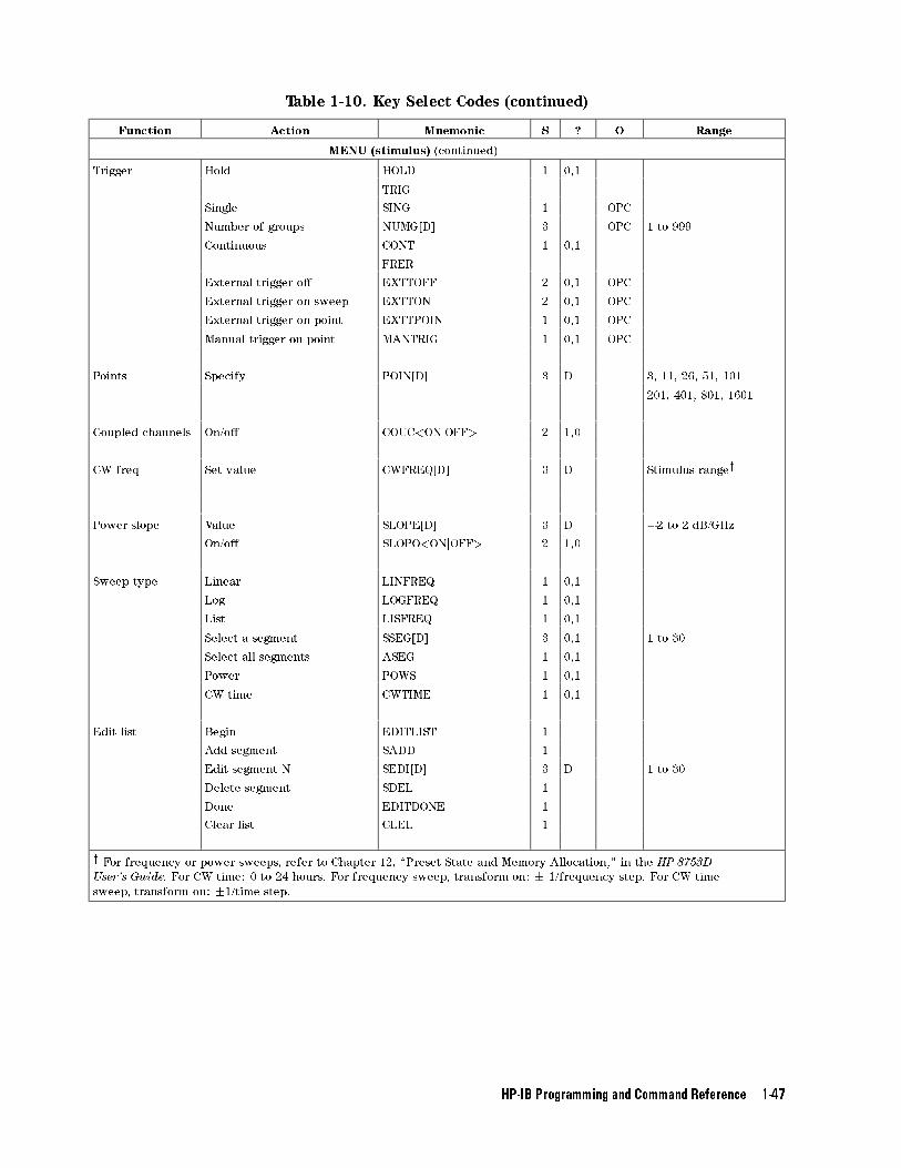
Table 1-10. Key Select Codes (continued)
Function Action Mnemonic S ? O Range
MENU (stimulus) (continued)
Trigger Hold HOLD 1 0,1
TRIG
Single SING 1 OPC
Number of groups NUMG[D] 3 OPC 1 to 999
Continuous CONT 1 0,1
FRER
External trigger o� EXTTOFF 2 0,1 OPC
External trigger on sweep EXTTON 2 0,1 OPC
External trigger on point EXTTPOIN 1 0,1 OPC
Manual trigger on point MANTRIG 1 0,1 OPC
Points Specify POIN[D] 3 D 3, 11, 26, 51, 101
201, 401, 801, 1601
Coupled channels On/o� COUC<ONjOFF> 2 1,0
CW freq Set value CWFREQ[D] 3 D Stimulus rangey
Power slope Value SLOPE[D] 3 D �2 to 2 dB/GHz
On/o� SLOPO<ONjOFF> 2 1,0
Sweep type Linear LINFREQ 1 0,1
Log LOGFREQ 1 0,1
List LISFREQ 1 0,1
Select a segment SSEG[D] 3 0,1 1 to 30
Select all segments ASEG 1 0,1
Power POWS 1 0,1
CW time CWTIME 1 0,1
Edit list Begin EDITLIST 1
Add segment SADD 1
Edit segment N SEDI[D] 3 D 1 to 30
Delete segment SDEL 1
Done EDITDONE 1
Clear list CLEL 1
y For frequency or power sweeps, refer to Chapter 12, \Preset State and Memory Allocation," in the HP 8753D
User's Guide. For CW time: 0 to 24 hours. For frequency sweep, transform on: � 1/frequency step. For CW time
sweep, transform on: �1/time step.
HP-IB Programming and Command Reference 1-47
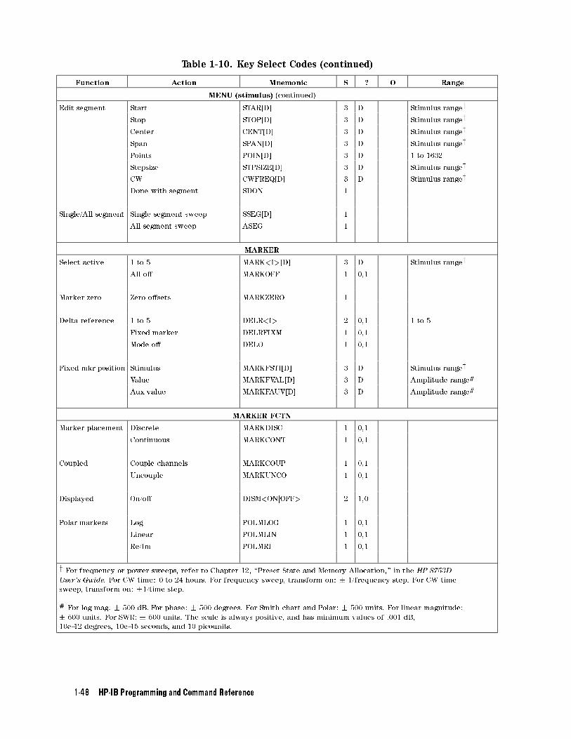
Table 1-10. Key Select Codes (continued)
Function Action Mnemonic S ? O Range
MENU (stimulus) (continued)
Edit segment Start STAR[D] 3 D Stimulus rangey
Stop STOP[D] 3 D Stimulus rangey
Center CENT[D] 3 D Stimulus rangey
Span SPAN[D] 3 D Stimulus rangey
Points POIN[D] 3 D 1 to 1632
Stepsize STPSIZE[D] 3 D Stimulus rangey
CW CWFREQ[D] 3 D Stimulus rangey
Done with segment SDON 1
Single/All segment Single segment sweep SSEG[D] 1
All segment sweep ASEG 1
MARKER
Select active 1 to 5 MARK<I>[D] 3 D Stimulus rangey
All o� MARKOFF 1 0,1
Marker zero Zero o�sets MARKZERO 1
Delta reference 1 to 5 DELR<I> 2 0,1 1 to 5
Fixed marker DELRFIXM 1 0,1
Mode o� DELO 1 0,1
Fixed mkr position Stimulus MARKFSTI[D] 3 D Stimulus rangey
Value MARKFVAL[D] 3 D Amplitude range#
Aux value MARKFAUV[D] 3 D Amplitude range#
MARKER FCTN
Marker placement Discrete MARKDISC 1 0,1
Continuous MARKCONT 1 0,1
Coupled Couple channels MARKCOUP 1 0,1
Uncouple MARKUNCO 1 0,1
Displayed On/o� DISM<ONjOFF> 2 1,0
Polar markers Log POLMLOG 1 0,1
Linear POLMLIN 1 0,1
Re/Im POLMRI 1 0,1
y For frequency or power sweeps, refer to Chapter 12, \Preset State and Memory Allocation," in the HP 8753D
User's Guide. For CW time: 0 to 24 hours. For frequency sweep, transform on: � 1/frequency step. For CW time
sweep, transform on: �1/time step.
# For log mag: � 500 dB. For phase: � 500 degrees. For Smith chart and Polar: � 500 units. For linear magnitude:
� 500 units. For SWR: � 500 units. The scale is always positive, and has minimum values of .001 dB,
10e-12 degrees, 10e-15 seconds, and 10 picounits.
1-48 HP-IB Programming and Command Reference
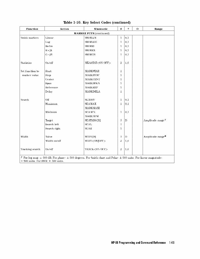
Table 1-10. Key Select Codes (continued)
Function Action Mnemonic S ? O Range
MARKER FCTN (continued)
Smith markers Linear SMIMLIN 1 0,1
Log SMIMLOG 1 0,1
Re/Im SMIMRI 1 0,1
R+jX SMIMRX 1 0,1
G+jB SMIMGB 1 0,1
Statistics On/o� MEASTAT<ONjOFF> 2 1,0
Set function to Start MARKSTAR 1
marker value Stop MARKSTOP 1
Center MARKCENT 1
Span MARKSPAN 1
Reference MARKREF 1
Delay MARKDELA 1
Search O� SEAOFF 1 0,1
Maximum SEAMAX 1 0,1
MARKMAXI
Minimum SEAMIN 1 0,1
MARKMINI
Target SEATARG[D] 3 D Amplitude range#
Search left SEAL 1
Search right SEAR 1
Width Value WIDV[D] 3 D Amplitude range#
Width on/o� WIDT<ONjOFF> 2 1,0
Tracking search On/o� TRACK<ONjOFF> 2 1,0
# For log mag: � 500 dB. For phase: � 500 degrees. For Smith chart and Polar: � 500 units. For linear magnitude:
� 500 units. For SWR: � 500 units.
HP-IB Programming and Command Reference 1-49
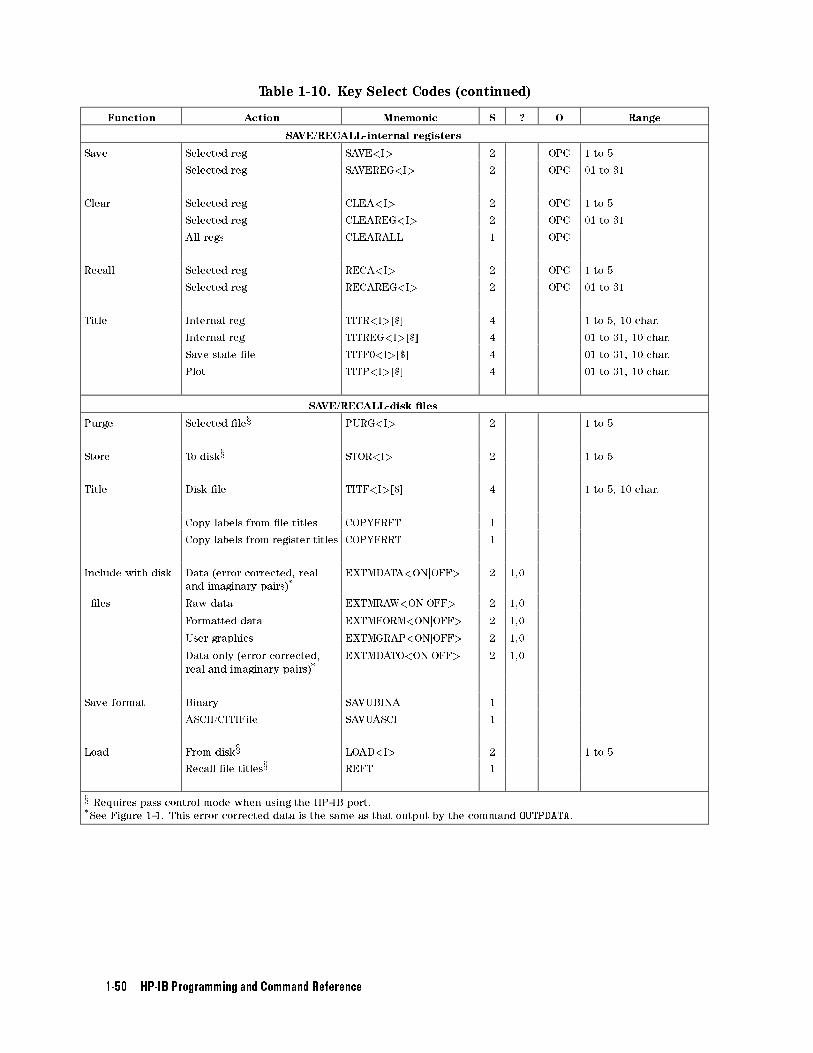
Table 1-10. Key Select Codes (continued)
Function Action Mnemonic S ? O Range
SAVE/RECALL-internal registers
Save Selected reg SAVE<I> 2 OPC 1 to 5
Selected reg SAVEREG<I> 2 OPC 01 to 31
Clear Selected reg CLEA<I> 2 OPC 1 to 5
Selected reg CLEAREG<I> 2 OPC 01 to 31
All regs CLEARALL 1 OPC
Recall Selected reg RECA<I> 2 OPC 1 to 5
Selected reg RECAREG<I> 2 OPC 01 to 31
Title Internal reg TITR<I>[$] 4 1 to 5, 10 char.
Internal reg TITREG<I>[$] 4 01 to 31, 10 char.
Save state �le TITF0<I>[$] 4 01 to 31, 10 char.
Plot TITP<I>[$] 4 01 to 31, 10 char.
SAVE/RECALL-disk �les
Purge Selected �lex PURG<I> 2 1 to 5
Store To diskx STOR<I> 2 1 to 5
Title Disk �le TITF<I>[$] 4 1 to 5, 10 char.
Copy labels from �le titles COPYFRFT 1
Copy labels from register titles COPYFRRT 1
Include with disk Data (error corrected, real
and imaginary pairs)*EXTMDATA<ONjOFF> 2 1,0
�les Raw data EXTMRAW<ONjOFF> 2 1,0
Formatted data EXTMFORM<ONjOFF> 2 1,0
User graphics EXTMGRAP<ONjOFF> 2 1,0
Data only (error corrected,
real and imaginary pairs)*EXTMDATO<ONjOFF> 2 1,0
Save format Binary SAVUBINA 1
ASCII/CITIFile SAVUASCI 1
Load From diskx LOAD<I> 2 1 to 5
Recall �le titlesx REFT 1
x Requires pass control mode when using the HP-IB port.*See Figure 1-1. This error corrected data is the same as that output by the command OUTPDATA.
1-50 HP-IB Programming and Command Reference
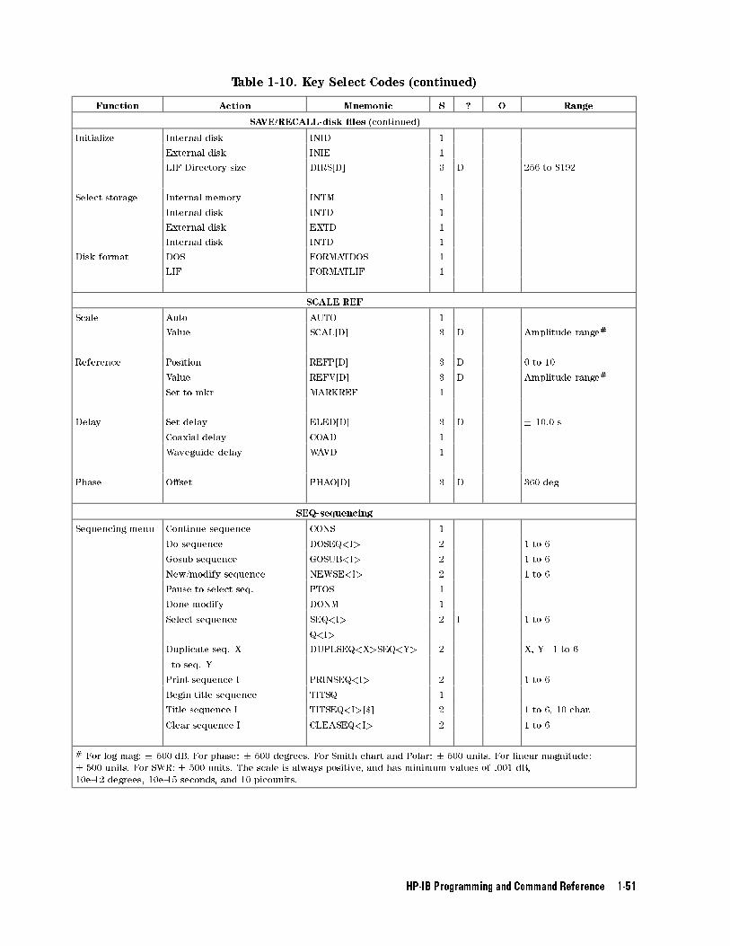
Table 1-10. Key Select Codes (continued)
Function Action Mnemonic S ? O Range
SAVE/RECALL-disk �les (continued)
Initialize Internal disk INID 1
External disk INIE 1
LIF Directory size DIRS[D] 3 D 256 to 8192
Select storage Internal memory INTM 1
Internal disk INTD 1
External disk EXTD 1
Internal disk INTD 1
Disk format DOS FORMATDOS 1
LIF FORMATLIF 1
SCALE REF
Scale Auto AUTO 1
Value SCAL[D] 3 D Amplitude range#
Reference Position REFP[D] 3 D 0 to 10
Value REFV[D] 3 D Amplitude range#
Set to mkr MARKREF 1
Delay Set delay ELED[D] 3 D � 10.0 s
Coaxial delay COAD 1
Waveguide delay WAVD 1
Phase O�set PHAO[D] 3 D 360 deg
SEQ-sequencing
Sequencing menu Continue sequence CONS 1
Do sequence DOSEQ<I> 2 1 to 6
Gosub sequence GOSUB<I> 2 1 to 6
New/modify sequence NEWSE<I> 2 1 to 6
Pause to select seq. PTOS 1
Done modify DONM 1
Select sequence SEQ<I> 2 I 1 to 6
Q<I>
Duplicate seq. X DUPLSEQ<X>SEQ<Y> 2 X, Y=1 to 6
to seq. Y
Print sequence I PRINSEQ<I> 2 1 to 6
Begin title sequence TITSQ 1
Title sequence I TITSEQ<I>[$] 2 1 to 6, 10 char.
Clear sequence I CLEASEQ<I> 2 1 to 6
# For log mag: � 500 dB. For phase: � 500 degrees. For Smith chart and Polar: � 500 units. For linear magnitude:
� 500 units. For SWR: � 500 units. The scale is always positive, and has minimum values of .001 dB,
10e-12 degrees, 10e-15 seconds, and 10 picounits.
HP-IB Programming and Command Reference 1-51
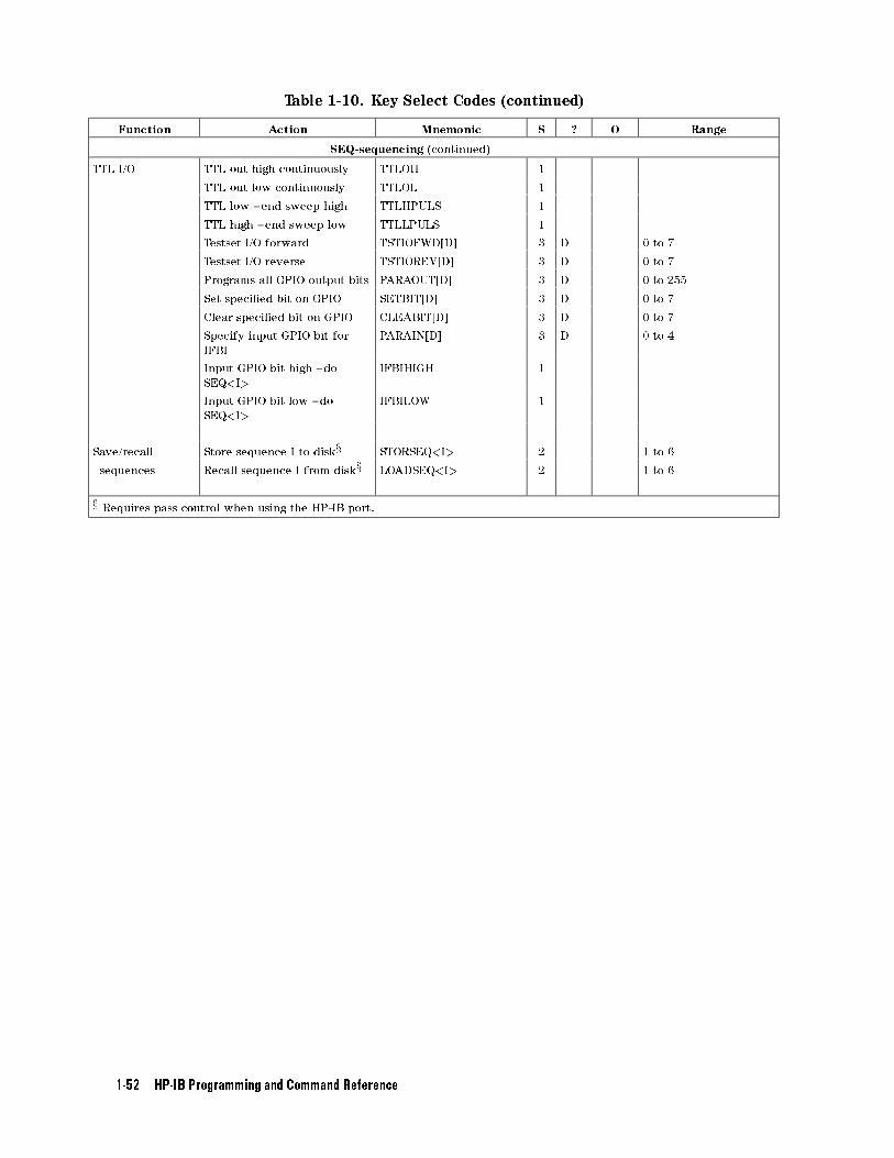
Table 1-10. Key Select Codes (continued)
Function Action Mnemonic S ? O Range
SEQ-sequencing (continued)
TTL I/O TTL out high continuously TTLOH 1
TTL out low continuously TTLOL 1
TTL low - end sweep high TTLHPULS 1
TTL high - end sweep low TTLLPULS 1
Testset I/O forward TSTIOFWD[D] 3 D 0 to 7
Testset I/O reverse TSTIOREV[D] 3 D 0 to 7
Programs all GPIO output bits PARAOUT[D] 3 D 0 to 255
Set speci�ed bit on GPIO SETBIT[D] 3 D 0 to 7
Clear speci�ed bit on GPIO CLEABIT[D] 3 D 0 to 7
Specify input GPIO bit for
IFBI
PARAIN[D] 3 D 0 to 4
Input GPIO bit high - do
SEQ<I>
IFBIHIGH 1
Input GPIO bit low - do
SEQ<I>
IFBILOW 1
Save/recall Store sequence I to diskx STORSEQ<I> 2 1 to 6
sequences Recall sequence I from diskx LOADSEQ<I> 2 1 to 6
x Requires pass control when using the HP-IB port.
1-52 HP-IB Programming and Command Reference
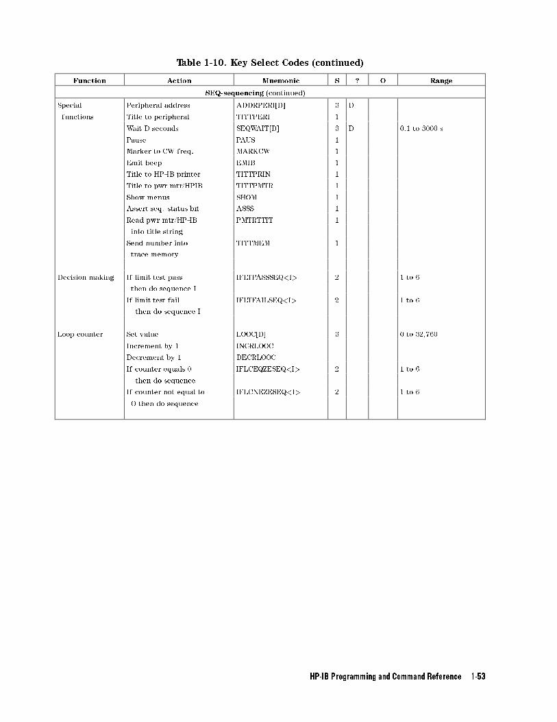
Table 1-10. Key Select Codes (continued)
Function Action Mnemonic S ? O Range
SEQ-sequencing (continued)
Special Peripheral address ADDRPERI[D] 3 D
functions Title to peripheral TITTPERI 1
Wait D seconds SEQWAIT[D] 3 D 0.1 to 3000 s
Pause PAUS 1
Marker to CW freq. MARKCW 1
Emit beep EMIB 1
Title to HP-IB printer TITTPRIN 1
Title to pwr mtr/HPIB TITTPMTR 1
Show menus SHOM 1
Assert seq. status bit ASSS 1
Read pwr mtr/HP-IB PMTRTTIT 1
into title string
Send number into TITTMEM 1
trace memory
Decision making If limit test pass IFLTPASSSEQ<I> 2 1 to 6
then do sequence I
If limit test fail IFLTFAILSEQ<I> 2 1 to 6
then do sequence I
Loop counter Set value LOOC[D] 3 0 to 32,760
Increment by 1 INCRLOOC
Decrement by 1 DECRLOOC
If counter equals 0 IFLCEQZESEQ<I> 2 1 to 6
then do sequence
If counter not equal to IFLCNEZESEQ<I> 2 1 to 6
O then do sequence
HP-IB Programming and Command Reference 1-53
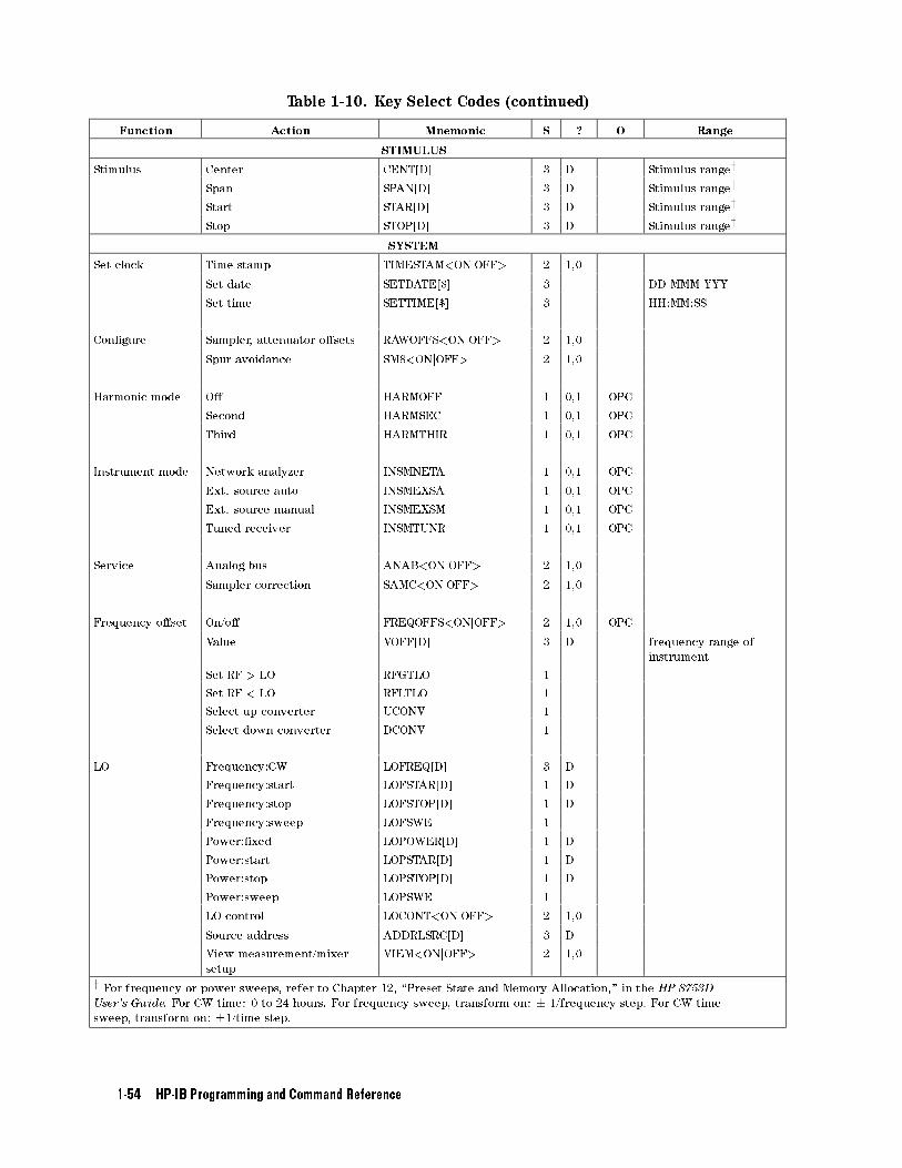
Table 1-10. Key Select Codes (continued)
Function Action Mnemonic S ? O Range
STIMULUS
Stimulus Center CENT[D] 3 D Stimulus rangey
Span SPAN[D] 3 D Stimulus rangey
Start STAR[D] 3 D Stimulus rangey
Stop STOP[D] 3 D Stimulus rangey
SYSTEM
Set clock Time stamp TIMESTAM<ONjOFF> 2 1,0
Set date SETDATE[$] 3 DD MMM YYY
Set time SETTIME[$] 3 HH:MM:SS
Con�gure Sampler, attenuator o�sets RAWOFFS<ONjOFF> 2 1,0
Spur avoidance SM8<ONjOFF> 2 1,0
Harmonic mode O� HARMOFF 1 0,1 OPC
Second HARMSEC 1 0,1 OPC
Third HARMTHIR 1 0,1 OPC
Instrument mode Network analyzer INSMNETA 1 0,1 OPC
Ext. source auto INSMEXSA 1 0,1 OPC
Ext. source manual INSMEXSM 1 0,1 OPC
Tuned receiver INSMTUNR 1 0,1 OPC
Service Analog bus ANAB<ONjOFF> 2 1,0
Sampler correction SAMC<ONjOFF> 2 1,0
Frequency o�set On/o� FREQOFFS<ONjOFF> 2 1,0 OPC
Value VOFF[D] 3 D frequency range of
instrument
Set RF > LO RFGTLO 1
Set RF < LO RFLTLO 1
Select up converter UCONV 1
Select down converter DCONV 1
LO Frequency:CW LOFREQ[D] 3 D
Frequency:start LOFSTAR[D] 1 D
Frequency:stop LOFSTOP[D] 1 D
Frequency:sweep LOFSWE 1
Power:�xed LOPOWER[D] 1 D
Power:start LOPSTAR[D] 1 D
Power:stop LOPSTOP[D] 1 D
Power:sweep LOPSWE 1
LO control LOCONT<ONjOFF> 2 1,0
Source address ADDRLSRC[D] 3 D
View measurement/mixer
setup
VIEM<ONjOFF> 2 1,0
y For frequency or power sweeps, refer to Chapter 12, \Preset State and Memory Allocation," in the HP 8753D
User's Guide. For CW time: 0 to 24 hours. For frequency sweep, transform on: � 1/frequency step. For CW time
sweep, transform on: �1/time step.
1-54 HP-IB Programming and Command Reference
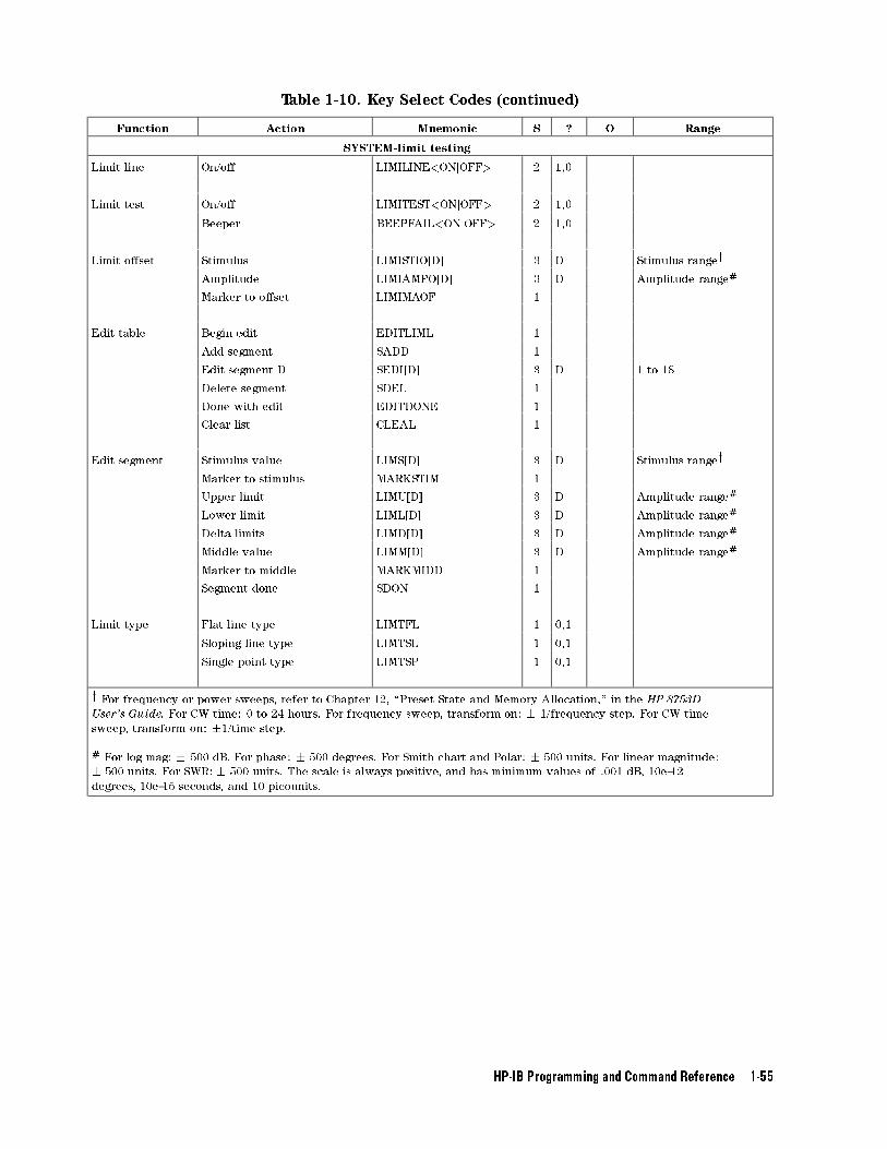
Table 1-10. Key Select Codes (continued)
Function Action Mnemonic S ? O Range
SYSTEM-limit testing
Limit line On/o� LIMILINE<ONjOFF> 2 1,0
Limit test On/o� LIMITEST<ONjOFF> 2 1,0
Beeper BEEPFAIL<ONjOFF> 2 1,0
Limit o�set Stimulus LIMISTIO[D] 3 D Stimulus rangey
Amplitude LIMIAMPO[D] 3 D Amplitude range#
Marker to o�set LIMIMAOF 1
Edit table Begin edit EDITLIML 1
Add segment SADD 1
Edit segment D SEDI[D] 3 D 1 to 18
Delete segment SDEL 1
Done with edit EDITDONE 1
Clear list CLEAL 1
Edit segment Stimulus value LIMS[D] 3 D Stimulus rangey
Marker to stimulus MARKSTIM 1
Upper limit LIMU[D] 3 D Amplitude range#
Lower limit LIML[D] 3 D Amplitude range#
Delta limits LIMD[D] 3 D Amplitude range#
Middle value LIMM[D] 3 D Amplitude range#
Marker to middle MARKMIDD 1
Segment done SDON 1
Limit type Flat line type LIMTFL 1 0,1
Sloping line type LIMTSL 1 0,1
Single point type LIMTSP 1 0,1
y For frequency or power sweeps, refer to Chapter 12, \Preset State and Memory Allocation," in the HP 8753D
User's Guide. For CW time: 0 to 24 hours. For frequency sweep, transform on: � 1/frequency step. For CW time
sweep, transform on: �1/time step.
# For log mag: � 500 dB. For phase: � 500 degrees. For Smith chart and Polar: � 500 units. For linear magnitude:
� 500 units. For SWR: � 500 units. The scale is always positive, and has minimum values of .001 dB, 10e-12
degrees, 10e-15 seconds, and 10 picounits.
HP-IB Programming and Command Reference 1-55
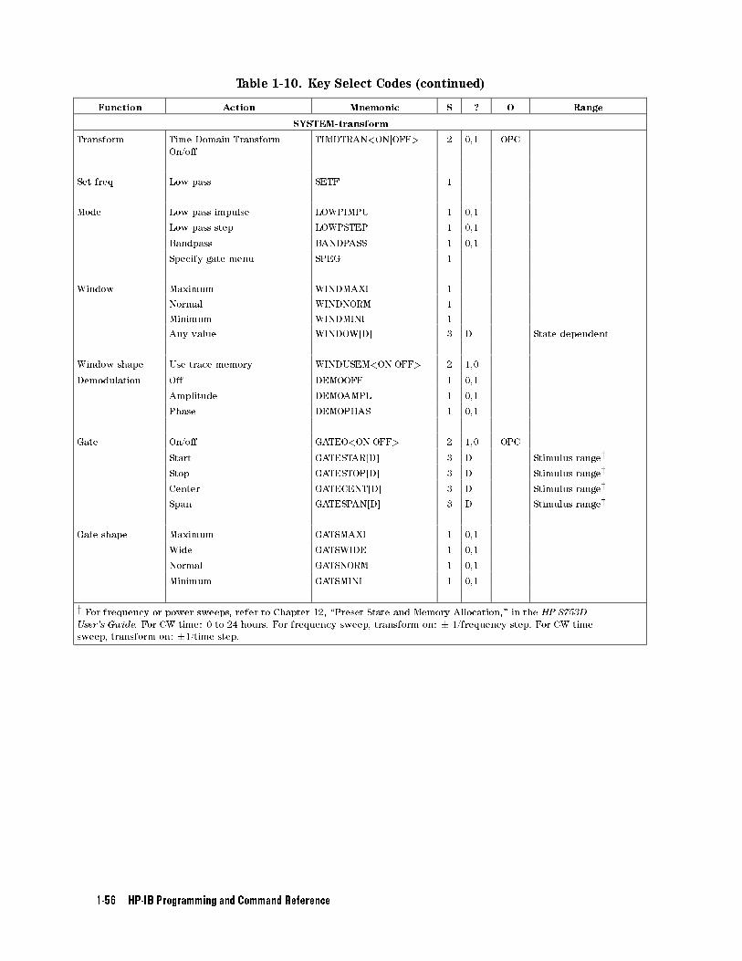
Table 1-10. Key Select Codes (continued)
Function Action Mnemonic S ? O Range
SYSTEM-transform
Transform Time Domain Transform
On/o�
TIMDTRAN<ONjOFF> 2 0,1 OPC
Set freq Low pass SETF 1
Mode Low pass impulse LOWPIMPU 1 0,1
Low pass step LOWPSTEP 1 0,1
Bandpass BANDPASS 1 0,1
Specify gate menu SPEG 1
Window Maximum WINDMAXI 1
Normal WINDNORM 1
Minimum WINDMINI 1
Any value WINDOW[D] 3 D State dependent
Window shape Use trace memory WINDUSEM<ONjOFF> 2 1,0
Demodulation O� DEMOOFF 1 0,1
Amplitude DEMOAMPL 1 0,1
Phase DEMOPHAS 1 0,1
Gate On/o� GATEO<ONjOFF> 2 1,0 OPC
Start GATESTAR[D] 3 D Stimulus rangey
Stop GATESTOP[D] 3 D Stimulus rangey
Center GATECENT[D] 3 D Stimulus rangey
Span GATESPAN[D] 3 D Stimulus rangey
Gate shape Maximum GATSMAXI 1 0,1
Wide GATSWIDE 1 0,1
Normal GATSNORM 1 0,1
Minimum GATSMINI 1 0,1
y For frequency or power sweeps, refer to Chapter 12, \Preset State and Memory Allocation," in the HP 8753D
User's Guide. For CW time: 0 to 24 hours. For frequency sweep, transform on: � 1/frequency step. For CW time
sweep, transform on: �1/time step.
1-56 HP-IB Programming and Command Reference
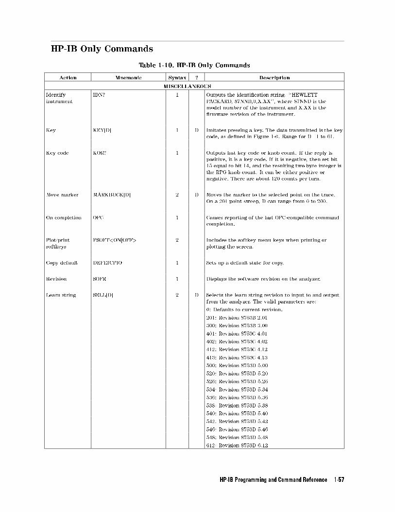
HP-IB Only Commands
Table 1-10. HP-IB Only Commands
Action Mnemonic Syntax ? Description
MISCELLANEOUS
Identify
instrument
IDN? 1 Outputs the identi�cation string: ``HEWLETT
PACKARD, 87NND,0,X.XX'', where 87NND is the
model number of the instrument and X.XX is the
�rmware revision of the instrument.
Key KEY[D] 1 D Imitates pressing a key. The data transmitted is the key
code, as de�ned in Figure 1-6. Range for D=1 to 61.
Key code KOR? 1 Outputs last key code or knob count. If the reply is
positive, it is a key code. If it is negative, then set bit
15 equal to bit 14, and the resulting two byte integer is
the RPG knob count. It can be either positive or
negative. There are about 120 counts per turn.
Move marker MARKBUCK[D] 2 D Moves the marker to the selected point on the trace.
On a 201 point sweep, D can range from 0 to 200.
On completion OPC 1 Causes reporting of the last OPC-compatible command
completion.
Plot/print
softkeys
PSOFT<ONjOFF> 2 Includes the softkey menu keys when printing or
plotting the screen.
Copy default DEFLTCPIO 1 Sets up a default state for copy.
Revision SOFR 1 Displays the software revision on the analyzer.
Learn string SELL[D] 2 D Selects the learn string revision to input to and output
from the analyzer. The valid parameters are:
0: Defaults to current revision.
201: Revision 8753B 2.01
300: Revision 8753B 3.00
401: Revision 8753C 4.01
402: Revision 8753C 4.02
412: Revision 8753C 4.12
413: Revision 8753C 4.13
500: Revision 8753D 5.00
520: Revision 8753D 5.20
526: Revision 8753D 5.26
534: Revision 8753D 5.34
536: Revision 8753D 5.36
538: Revision 8753D 5.38
540: Revision 8753D 5.40
542: Revision 8753D 5.42
546: Revision 8753D 5.46
548: Revision 8753D 5.48
612: Revision 8753D 6.12
HP-IB Programming and Command Reference 1-57
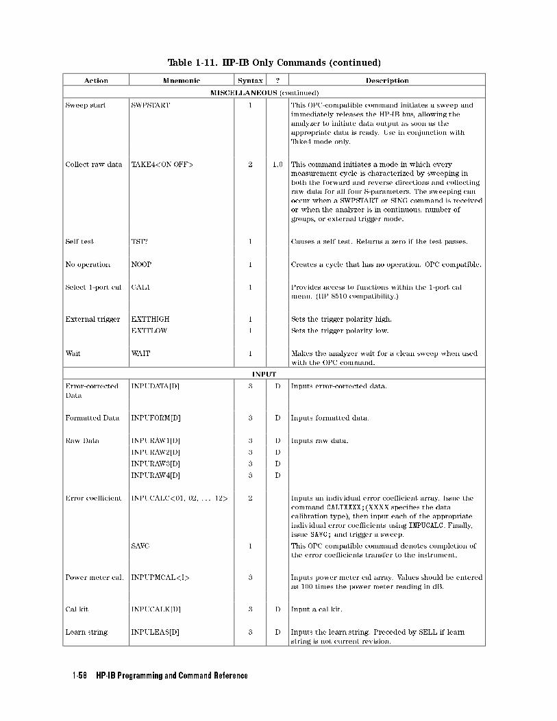
Table 1-11. HP-IB Only Commands (continued)
Action Mnemonic Syntax ? Description
MISCELLANEOUS (continued)
Sweep start SWPSTART 1 This OPC-compatible command initiates a sweep and
immediately releases the HP-IB bus, allowing the
analyzer to initiate data output as soon as the
appropriate data is ready. Use in conjunction with
Take4 mode only.
Collect raw data TAKE4<ONjOFF> 2 1,0 This command initiates a mode in which every
measurement cycle is characterized by sweeping in
both the forward and reverse directions and collecting
raw data for all four S-parameters. The sweeping can
occur when a SWPSTART or SING command is received
or when the analyzer is in continuous, number of
groups, or external trigger mode.
Self test TST? 1 Causes a self test. Returns a zero if the test passes.
No operation NOOP 1 Creates a cycle that has no operation. OPC compatible.
Select 1-port cal CAL1 1 Provides access to functions within the 1-port cal
menu. (HP 8510 compatibility.)
External trigger EXTTHIGH 1 Sets the trigger polarity high.
EXTTLOW 1 Sets the trigger polarity low.
Wait WAIT 1 Makes the analyzer wait for a clean sweep when used
with the OPC command.
INPUT
Error-corrected
Data
INPUDATA[D] 3 D Inputs error-corrected data.
Formatted Data INPUFORM[D] 3 D Inputs formatted data.
Raw Data INPURAW1[D] 3 D Inputs raw data.
INPURAW2[D] 3 D
INPURAW3[D] 3 D
INPURAW4[D] 3 D
Error coe�cient INPUCALC<01, 02, . . . 12> 2 Inputs an individual error coe�cient array. Issue the
command CALIXXXX;(XXXX speci�es the data
calibration type), then input each of the appropriate
individual error coe�cients using INPUCALC. Finally,
issue SAVC; and trigger a sweep.
SAVC 1 This OPC compatible command denotes completion of
the error coe�cients transfer to the instrument.
Power meter cal. INPUPMCAL<I> 3 Inputs power meter cal array. Values should be entered
as 100 times the power meter reading in dB.
Cal kit INPUCALK[D] 3 D Input a cal kit.
Learn string INPULEAS[D] 3 D Inputs the learn string. Preceded by SELL if learn
string is not current revision.
1-58 HP-IB Programming and Command Reference
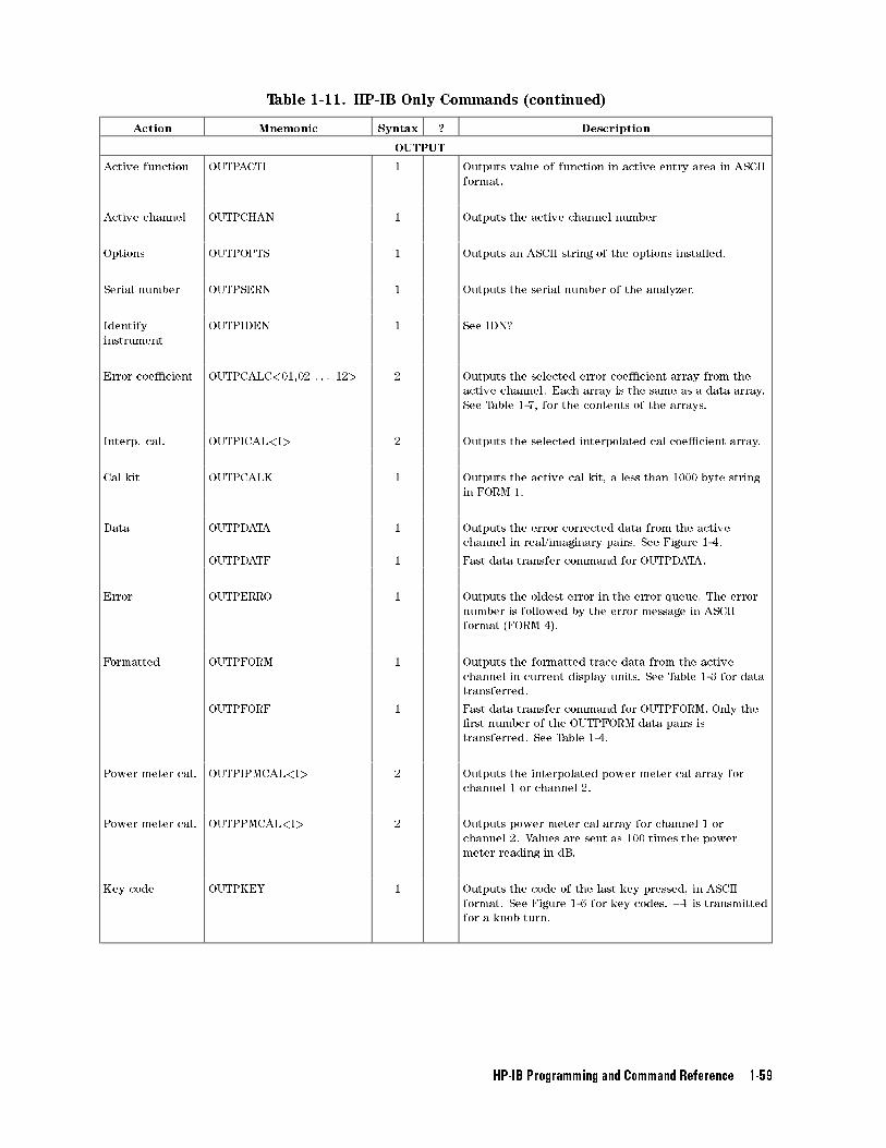
Table 1-11. HP-IB Only Commands (continued)
Action Mnemonic Syntax ? Description
OUTPUT
Active function OUTPACTI 1 Outputs value of function in active entry area in ASCII
format.
Active channel OUTPCHAN 1 Outputs the active channel number.
Options OUTPOPTS 1 Outputs an ASCII string of the options installed.
Serial number OUTPSERN 1 Outputs the serial number of the analyzer.
Identify
instrument
OUTPIDEN 1 See IDN?
Error coe�cient OUTPCALC<01,02 . . . 12> 2 Outputs the selected error coe�cient array from the
active channel. Each array is the same as a data array.
See Table 1-7, for the contents of the arrays.
Interp. cal. OUTPICAL<I> 2 Outputs the selected interpolated cal coe�cient array.
Cal kit OUTPCALK 1 Outputs the active cal kit, a less than 1000 byte string
in FORM 1.
Data OUTPDATA 1 Outputs the error corrected data from the active
channel in real/imaginary pairs. See Figure 1-4.
OUTPDATF 1 Fast data transfer command for OUTPDATA.
Error OUTPERRO 1 Outputs the oldest error in the error queue. The error
number is followed by the error message in ASCII
format (FORM 4).
Formatted OUTPFORM 1 Outputs the formatted trace data from the active
channel in current display units. See Table 1-3 for data
transferred.
OUTPFORF 1 Fast data transfer command for OUTPFORM. Only the
�rst number of the OUTPFORM data pairs is
transferred. See Table 1-4.
Power meter cal. OUTPIPMCAL<I> 2 Outputs the interpolated power meter cal array for
channel 1 or channel 2.
Power meter cal. OUTPPMCAL<I> 2 Outputs power meter cal array for channel 1 or
channel 2. Values are sent as 100 times the power
meter reading in dB.
Key code OUTPKEY 1 Outputs the code of the last key pressed, in ASCII
format. See Figure 1-6 for key codes. �1 is transmitted
for a knob turn.
HP-IB Programming and Command Reference 1-59
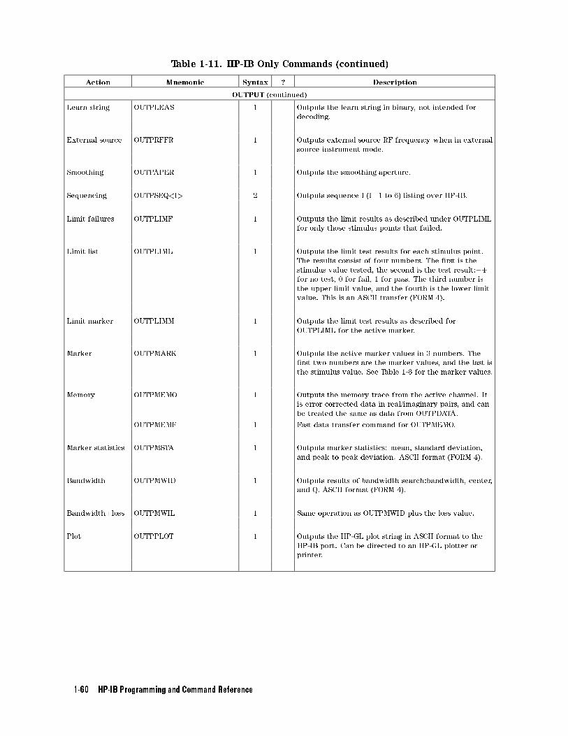
Table 1-11. HP-IB Only Commands (continued)
Action Mnemonic Syntax ? Description
OUTPUT (continued)
Learn string OUTPLEAS 1 Outputs the learn string in binary, not intended for
decoding.
External source OUTPRFFR 1 Outputs external source RF frequency when in external
source instrument mode.
Smoothing OUTPAPER 1 Outputs the smoothing aperture.
Sequencing OUTPSEQ<I> 2 Outputs sequence I (I=1 to 6) listing over HP-IB.
Limit failures OUTPLIMF 1 Outputs the limit results as described under OUTPLIML
for only those stimulus points that failed.
Limit list OUTPLIML 1 Outputs the limit test results for each stimulus point.
The results consist of four numbers. The �rst is the
stimulus value tested, the second is the test result:|1
for no test, 0 for fail, 1 for pass. The third number is
the upper limit value, and the fourth is the lower limit
value. This is an ASCII transfer (FORM 4).
Limit marker OUTPLIMM 1 Outputs the limit test results as described for
OUTPLIML for the active marker.
Marker OUTPMARK 1 Outputs the active marker values in 3 numbers. The
�rst two numbers are the marker values, and the last is
the stimulus value. See Table 1-3 for the marker values.
Memory OUTPMEMO 1 Outputs the memory trace from the active channel. It
is error corrected data in real/imaginary pairs, and can
be treated the same as data from OUTPDATA.
OUTPMEMF 1 Fast data transfer command for OUTPMEMO.
Marker statistics OUTPMSTA 1 Outputs marker statistics: mean, standard deviation,
and peak to peak deviation. ASCII format (FORM 4).
Bandwidth OUTPMWID 1 Outputs results of bandwidth search:bandwidth, center,
and Q. ASCII format (FORM 4).
Bandwidth+loss OUTPMWIL 1 Same operation as OUTPMWID plus the loss value.
Plot OUTPPLOT 1 Outputs the HP-GL plot string in ASCII format to the
HP-IB port. Can be directed to an HP-GL plotter or
printer.
1-60 HP-IB Programming and Command Reference
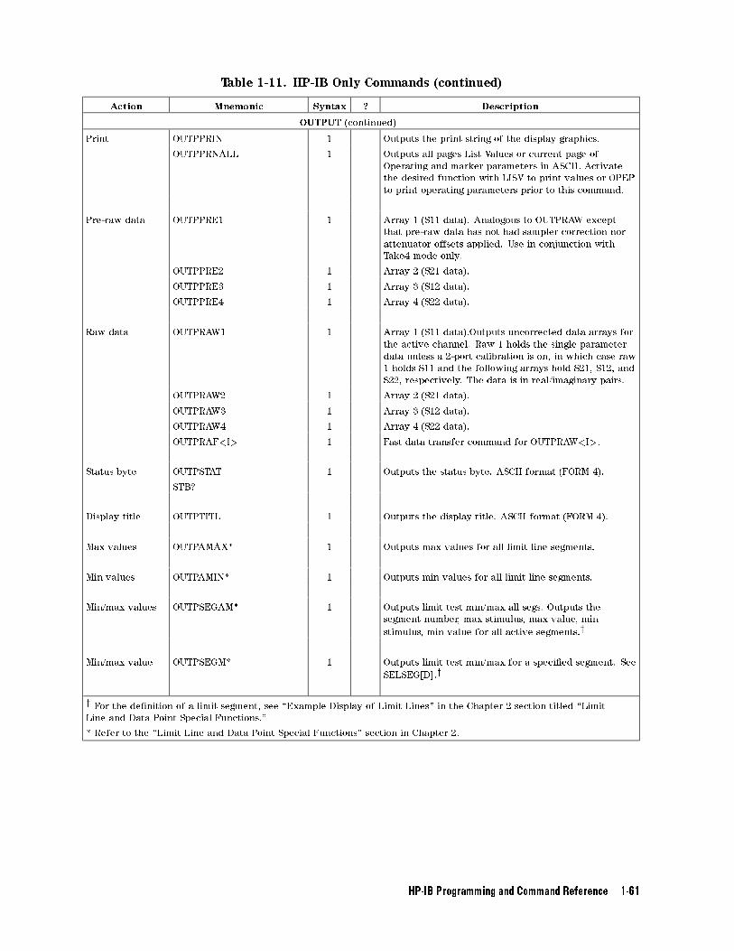
Table 1-11. HP-IB Only Commands (continued)
Action Mnemonic Syntax ? Description
OUTPUT (continued)
Print OUTPPRIN 1 Outputs the print string of the display graphics.
OUTPPRNALL 1 Outputs all pages List Values or current page of
Operating and marker parameters in ASCII. Activate
the desired function with LISV to print values or OPEP
to print operating parameters prior to this command.
Pre-raw data OUTPPRE1 1 Array 1 (S11 data). Analogous to OUTPRAW except
that pre-raw data has not had sampler correction nor
attenuator o�sets applied. Use in conjunction with
Take4 mode only.
OUTPPRE2 1 Array 2 (S21 data).
OUTPPRE3 1 Array 3 (S12 data).
OUTPPRE4 1 Array 4 (S22 data).
Raw data OUTPRAW1 1 Array 1 (S11 data).Outputs uncorrected data arrays for
the active channel. Raw 1 holds the single parameter
data unless a 2-port calibration is on, in which case raw
1 holds S11 and the following arrays hold S21, S12, and
S22, respectively. The data is in real/imaginary pairs.
OUTPRAW2 1 Array 2 (S21 data).
OUTPRAW3 1 Array 3 (S12 data).
OUTPRAW4 1 Array 4 (S22 data).
OUTPRAF<I> 1 Fast data transfer command for OUTPRAW<I>.
Status byte OUTPSTAT 1 Outputs the status byte. ASCII format (FORM 4).
STB?
Display title OUTPTITL 1 Outputs the display title. ASCII format (FORM 4).
Max values OUTPAMAX* 1 Outputs max values for all limit line segments.
Min values OUTPAMIN* 1 Outputs min values for all limit line segments.
Min/max values OUTPSEGAM* 1 Outputs limit test min/max all segs. Outputs the
segment number, max stimulus, max value, min
stimulus, min value for all active segments.y
Min/max value OUTPSEGM* 1 Outputs limit test min/max for a speci�ed segment. See
SELSEG[D].y
y For the de�nition of a limit segment, see \Example Display of Limit Lines" in the Chapter 2 section titled \Limit
Line and Data Point Special Functions."
* Refer to the \Limit Line and Data Point Special Functions" section in Chapter 2.
HP-IB Programming and Command Reference 1-61
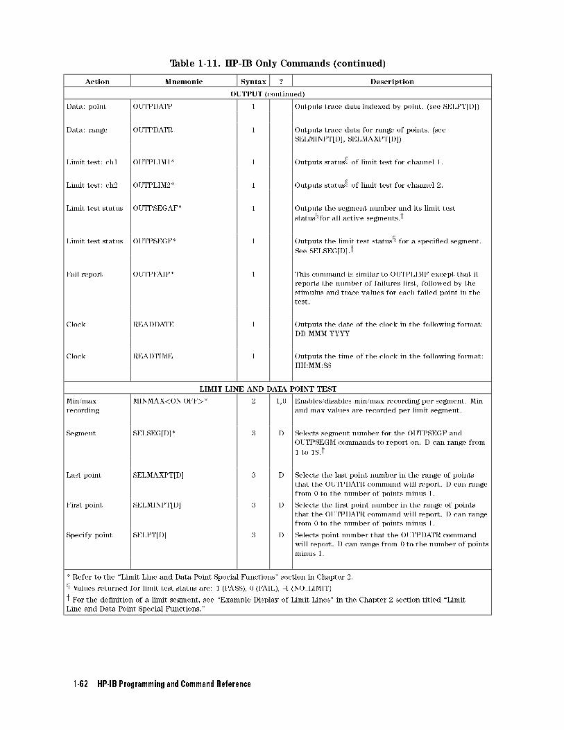
Table 1-11. HP-IB Only Commands (continued)
Action Mnemonic Syntax ? Description
OUTPUT (continued)
Data: point OUTPDATP 1 Outputs trace data indexed by point. (see SELPT[D])
Data: range OUTPDATR 1 Outputs trace data for range of points. (see
SELMINPT[D], SELMAXPT[D])
Limit test: ch1 OUTPLIM1* 1 Outputs statusx of limit test for channel 1.
Limit test: ch2 OUTPLIM2* 1 Outputs statusx of limit test for channel 2.
Limit test status OUTPSEGAF* 1 Outputs the segment number and its limit test
statusxfor all active segments.y
Limit test status OUTPSEGF* 1 Outputs the limit test statusx for a speci�ed segment.
See SELSEG[D].y
Fail report OUTPFAIP* 1 This command is similar to OUTPLIMF except that it
reports the number of failures �rst, followed by the
stimulus and trace values for each failed point in the
test.
Clock READDATE 1 Outputs the date of the clock in the following format:
DD MMM YYYY
Clock READTIME 1 Outputs the time of the clock in the following format:
HH:MM:SS
LIMIT LINE AND DATA POINT TEST
Min/max
recording
MINMAX<ONjOFF>* 2 1,0 Enables/disables min/max recording per segment. Min
and max values are recorded per limit segment.
Segment SELSEG[D]* 3 D Selects segment number for the OUTPSEGF and
OUTPSEGM commands to report on. D can range from
1 to 18.y
Last point SELMAXPT[D] 3 D Selects the last point number in the range of points
that the OUTPDATR command will report. D can range
from 0 to the number of points minus 1.
First point SELMINPT[D] 3 D Selects the �rst point number in the range of points
that the OUTPDATR command will report. D can range
from 0 to the number of points minus 1.
Specify point SELPT[D] 3 D Selects point number that the OUTPDATR command
will report. D can range from 0 to the number of points
minus 1.
* Refer to the \Limit Line and Data Point Special Functions" section in Chapter 2.
x Values returned for limit test status are: 1 (PASS), 0 (FAIL), -1 (NO LIMIT)
y For the de�nition of a limit segment, see \Example Display of Limit Lines" in the Chapter 2 section titled \Limit
Line and Data Point Special Functions."
1-62 HP-IB Programming and Command Reference
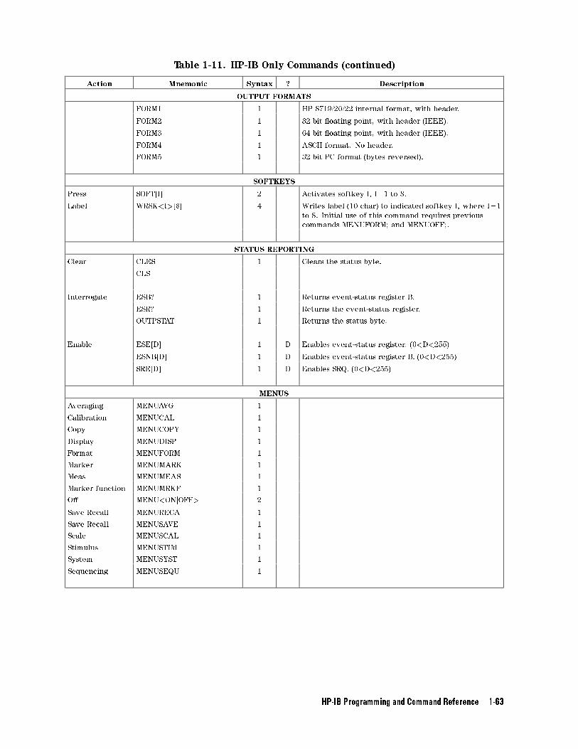
Table 1-11. HP-IB Only Commands (continued)
Action Mnemonic Syntax ? Description
OUTPUT FORMATS
FORM1 1 HP 8719/20/22 internal format, with header.
FORM2 1 32 bit oating point, with header (IEEE).
FORM3 1 64 bit oating point, with header (IEEE).
FORM4 1 ASCII format. No header.
FORM5 1 32 bit PC format (bytes reversed).
SOFTKEYS
Press SOFT[I] 2 Activates softkey I, I=1 to 8.
Label WRSK<I>[$] 4 Writes label (10 char) to indicated softkey I, where I=1
to 8. Initial use of this command requires previous
commands MENUFORM; and MENUOFF;.
STATUS REPORTING
Clear CLES 1 Clears the status byte.
CLS
Interrogate ESB? 1 Returns event-status register B.
ESR? 1 Returns the event-status register.
OUTPSTAT 1 Returns the status byte.
Enable ESE[D] 1 D Enables event-status register. (0<D<255)
ESNB[D] 1 D Enables event-status register B. (0<D<255)
SRE[D] 1 D Enables SRQ. (0<D<255)
MENUS
Averaging MENUAVG 1
Calibration MENUCAL 1
Copy MENUCOPY 1
Display MENUDISP 1
Format MENUFORM 1
Marker MENUMARK 1
Meas MENUMEAS 1
Marker function MENUMRKF 1
O� MENU<ONjOFF> 2
Save Recall MENURECA 1
Save Recall MENUSAVE 1
Scale MENUSCAL 1
Stimulus MENUSTIM 1
System MENUSYST 1
Sequencing MENUSEQU 1
HP-IB Programming and Command Reference 1-63
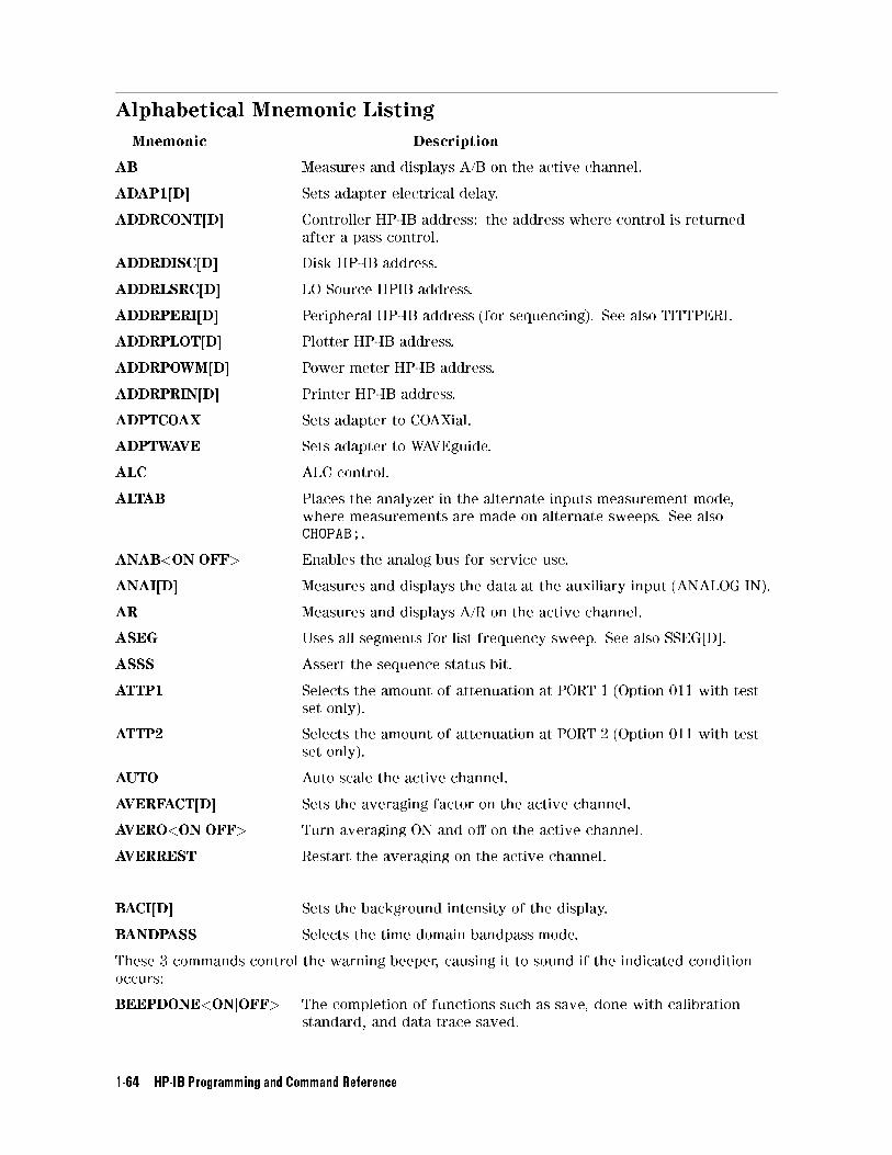
Alphabetical Mnemonic Listing
Mnemonic Description
AB Measures and displays A/B on the active channel.
ADAP1[D] Sets adapter electrical delay.
ADDRCONT[D] Controller HP-IB address: the address where control is returned
after a pass control.
ADDRDISC[D] Disk HP-IB address.
ADDRLSRC[D] LO Source HPIB address.
ADDRPERI[D] Peripheral HP-IB address (for sequencing). See also TITTPERI.
ADDRPLOT[D] Plotter HP-IB address.
ADDRPOWM[D] Power meter HP-IB address.
ADDRPRIN[D] Printer HP-IB address.
ADPTCOAX Sets adapter to COAXial.
ADPTWAVE Sets adapter to WAVEguide.
ALC ALC control.
ALTAB Places the analyzer in the alternate inputs measurement mode,
where measurements are made on alternate sweeps. See also
CHOPAB;.
ANAB<ONjOFF> Enables the analog bus for service use.
ANAI[D] Measures and displays the data at the auxiliary input (ANALOG IN).
AR Measures and displays A/R on the active channel.
ASEG Uses all segments for list frequency sweep. See also SSEG[D].
ASSS Assert the sequence status bit.
ATTP1 Selects the amount of attenuation at PORT 1 (Option 011 with test
set only).
ATTP2 Selects the amount of attenuation at PORT 2 (Option 011 with test
set only).
AUTO Auto scale the active channel.
AVERFACT[D] Sets the averaging factor on the active channel.
AVERO<ONjOFF> Turn averaging ON and o� on the active channel.
AVERREST Restart the averaging on the active channel.
BACI[D] Sets the background intensity of the display.
BANDPASS Selects the time domain bandpass mode.
These 3 commands control the warning beeper, causing it to sound if the indicated condition
occurs:
BEEPDONE<ONjOFF> The completion of functions such as save, done with calibration
standard, and data trace saved.
1-64 HP-IB Programming and Command Reference
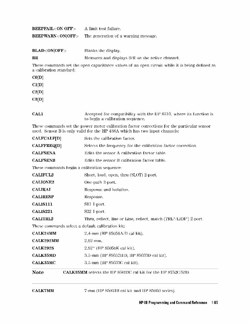
BEEPFAIL<ONjOFF> A limit test failure.
BEEPWARN<ONjOFF> The generation of a warning message.
BLAD<ONjOFF> Blanks the display.
BR Measures and displays B/R on the active channel.
These commands set the open capacitance values of an open circuit while it is being de�ned as
a calibration standard:
C0[D]
C1[D]
C2[D]
C3[D]
CAL1 Accepted for compatibility with the HP 8510, where its function is
to begin a calibration sequence.
These commands set the power meter calibration factor corrections for the particular sensor
used. Sensor B is only valid for the HP 438A which has two input channels:
CALFCALF[D] Sets the calibration factor.
CALFFREQ[D] Selects the frequency for the calibration factor correction.
CALFSENA Edits the sensor A calibration factor table.
CALFSENB Edits the sensor B calibration factor table.
These commands begin a calibration sequence:
CALIFUL2 Short, load, open, thru (SLOT) 2-port.
CALIONE2 One-path 2-port.
CALIRAI Response and isolation.
CALIRESP Response.
CALIS111 S11 1-port.
CALIS221 S22 1-port.
CALITRL2 Thru, re ect, line or Line, re ect, match (TRL*/LRM*) 2-port.
These commands select a default calibration kit:
CALK24MM 2.4-mm (HP 85056A/D cal kit).
CALK292MM 2.92-mm.
CALK292S 2.92* (HP 85056K cal kit).
CALK35MD 3.5-mm (HP 85052B/D, HP 85033D cal kit).
CALK35MC 3.5-mm (HP 85033C cal kit).
Note CALK35MM selects the HP 85033C cal kit for the HP 8752C/53D.
CALK7MM 7-mm (HP 85031B cal kit and HP 85050 series).
HP-IB Programming and Command Reference 1-65
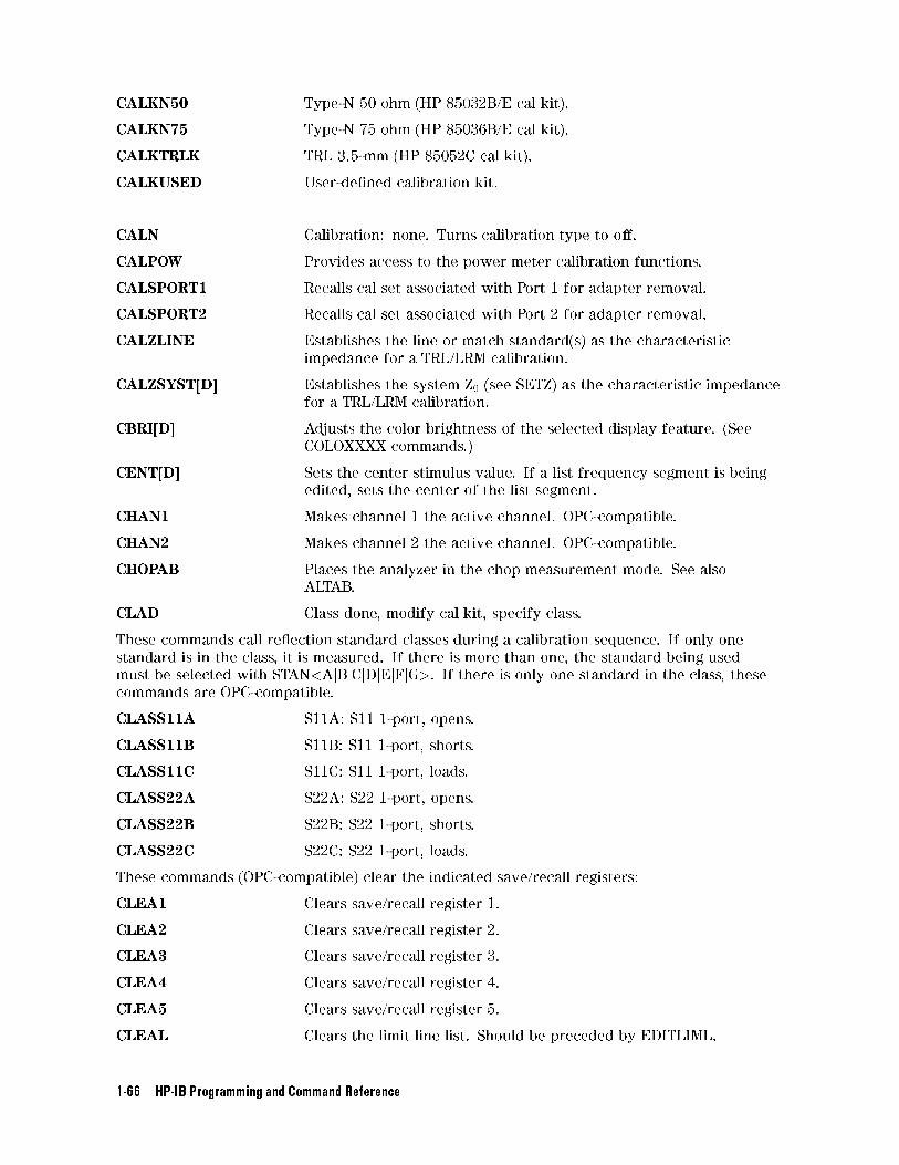
CALKN50 Type-N 50 ohm (HP 85032B/E cal kit).
CALKN75 Type-N 75 ohm (HP 85036B/E cal kit).
CALKTRLK TRL 3.5-mm (HP 85052C cal kit).
CALKUSED User-de�ned calibration kit.
CALN Calibration: none. Turns calibration type to o�.
CALPOW Provides access to the power meter calibration functions.
CALSPORT1 Recalls cal set associated with Port 1 for adapter removal.
CALSPORT2 Recalls cal set associated with Port 2 for adapter removal.
CALZLINE Establishes the line or match standard(s) as the characteristic
impedance for a TRL/LRM calibration.
CALZSYST[D] Establishes the system Z0 (see SETZ) as the characteristic impedance
for a TRL/LRM calibration.
CBRI[D] Adjusts the color brightness of the selected display feature. (See
COLOXXXX commands.)
CENT[D] Sets the center stimulus value. If a list frequency segment is being
edited, sets the center of the list segment.
CHAN1 Makes channel 1 the active channel. OPC-compatible.
CHAN2 Makes channel 2 the active channel. OPC-compatible.
CHOPAB Places the analyzer in the chop measurement mode. See also
ALTAB.
CLAD Class done, modify cal kit, specify class.
These commands call re ection standard classes during a calibration sequence. If only one
standard is in the class, it is measured. If there is more than one, the standard being used
must be selected with STAN<AjBjCjDjEjFjG>. If there is only one standard in the class, these
commands are OPC-compatible.
CLASS11A S11A: S11 1-port, opens.
CLASS11B S11B: S11 1-port, shorts.
CLASS11C S11C: S11 1-port, loads.
CLASS22A S22A: S22 1-port, opens.
CLASS22B S22B: S22 1-port, shorts.
CLASS22C S22C: S22 1-port, loads.
These commands (OPC-compatible) clear the indicated save/recall registers:
CLEA1 Clears save/recall register 1.
CLEA2 Clears save/recall register 2.
CLEA3 Clears save/recall register 3.
CLEA4 Clears save/recall register 4.
CLEA5 Clears save/recall register 5.
CLEAL Clears the limit line list. Should be preceded by EDITLIML.
1-66 HP-IB Programming and Command Reference
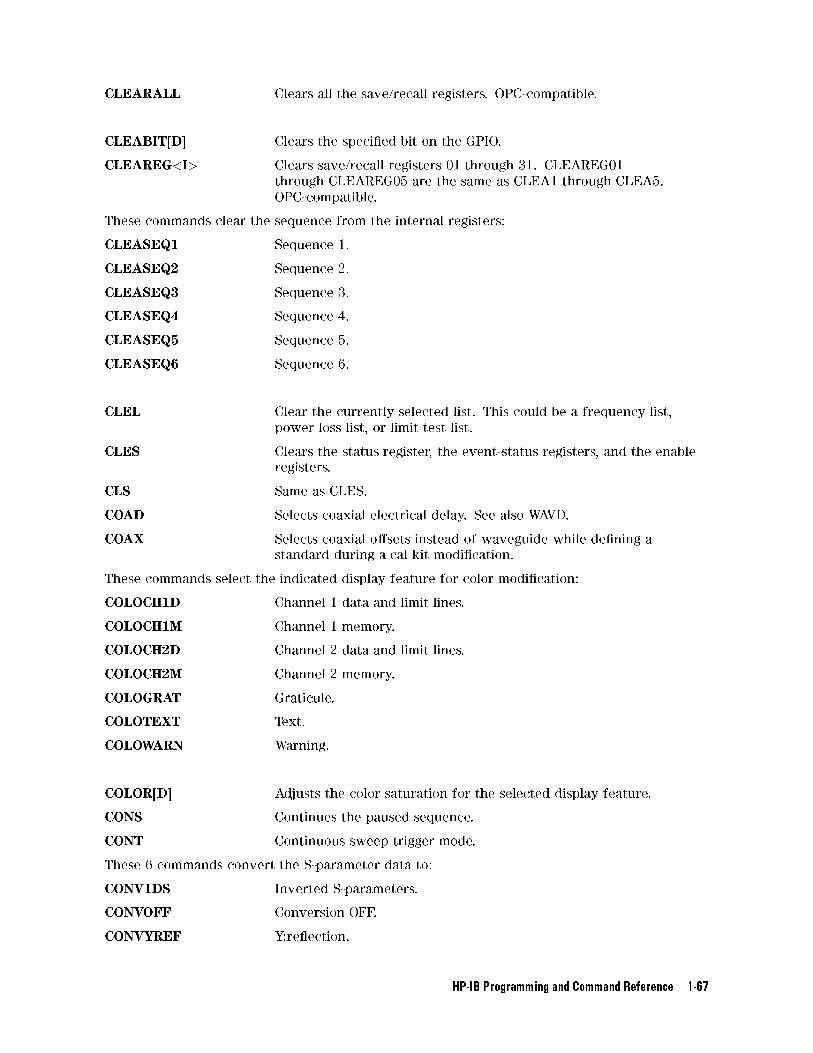
CLEARALL Clears all the save/recall registers. OPC-compatible.
CLEABIT[D] Clears the speci�ed bit on the GPIO.
CLEAREG<I> Clears save/recall registers 01 through 31. CLEAREG01
through CLEAREG05 are the same as CLEA1 through CLEA5.
OPC-compatible.
These commands clear the sequence from the internal registers:
CLEASEQ1 Sequence 1.
CLEASEQ2 Sequence 2.
CLEASEQ3 Sequence 3.
CLEASEQ4 Sequence 4.
CLEASEQ5 Sequence 5.
CLEASEQ6 Sequence 6.
CLEL Clear the currently selected list. This could be a frequency list,
power loss list, or limit test list.
CLES Clears the status register, the event-status registers, and the enable
registers.
CLS Same as CLES.
COAD Selects coaxial electrical delay. See also WAVD.
COAX Selects coaxial o�sets instead of waveguide while de�ning a
standard during a cal kit modi�cation.
These commands select the indicated display feature for color modi�cation:
COLOCH1D Channel 1 data and limit lines.
COLOCH1M Channel 1 memory.
COLOCH2D Channel 2 data and limit lines.
COLOCH2M Channel 2 memory.
COLOGRAT Graticule.
COLOTEXT Text.
COLOWARN Warning.
COLOR[D] Adjusts the color saturation for the selected display feature.
CONS Continues the paused sequence.
CONT Continuous sweep trigger mode.
These 6 commands convert the S-parameter data to:
CONV1DS Inverted S-parameters.
CONVOFF Conversion OFF.
CONVYREF Y:re ection.
HP-IB Programming and Command Reference 1-67
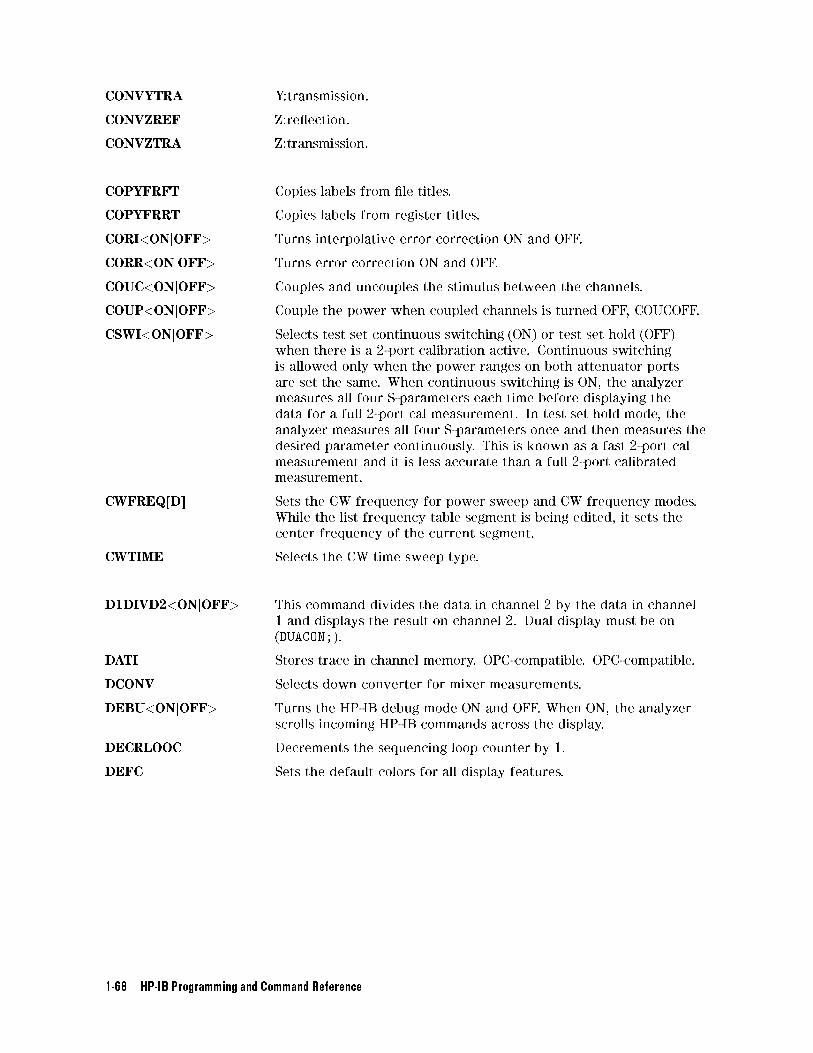
CONVYTRA Y:transmission.
CONVZREF Z:re ection.
CONVZTRA Z:transmission.
COPYFRFT Copies labels from �le titles.
COPYFRRT Copies labels from register titles.
CORI<ONjOFF> Turns interpolative error correction ON and OFF.
CORR<ONjOFF> Turns error correction ON and OFF.
COUC<ONjOFF> Couples and uncouples the stimulus between the channels.
COUP<ONjOFF> Couple the power when coupled channels is turned OFF, COUCOFF.
CSWI<ONjOFF> Selects test set continuous switching (ON) or test set hold (OFF)
when there is a 2-port calibration active. Continuous switching
is allowed only when the power ranges on both attenuator ports
are set the same. When continuous switching is ON, the analyzer
measures all four S-parameters each time before displaying the
data for a full 2-port cal measurement. In test set hold mode, the
analyzer measures all four S-parameters once and then measures the
desired parameter continuously. This is known as a fast 2-port cal
measurement and it is less accurate than a full 2-port calibrated
measurement.
CWFREQ[D] Sets the CW frequency for power sweep and CW frequency modes.
While the list frequency table segment is being edited, it sets the
center frequency of the current segment.
CWTIME Selects the CW time sweep type.
D1DIVD2<ONjOFF> This command divides the data in channel 2 by the data in channel
1 and displays the result on channel 2. Dual display must be on
(DUACON;).
DATI Stores trace in channel memory. OPC-compatible. OPC-compatible.
DCONV Selects down converter for mixer measurements.
DEBU<ONjOFF> Turns the HP-IB debug mode ON and OFF. When ON, the analyzer
scrolls incoming HP-IB commands across the display.
DECRLOOC Decrements the sequencing loop counter by 1.
DEFC Sets the default colors for all display features.
1-68 HP-IB Programming and Command Reference
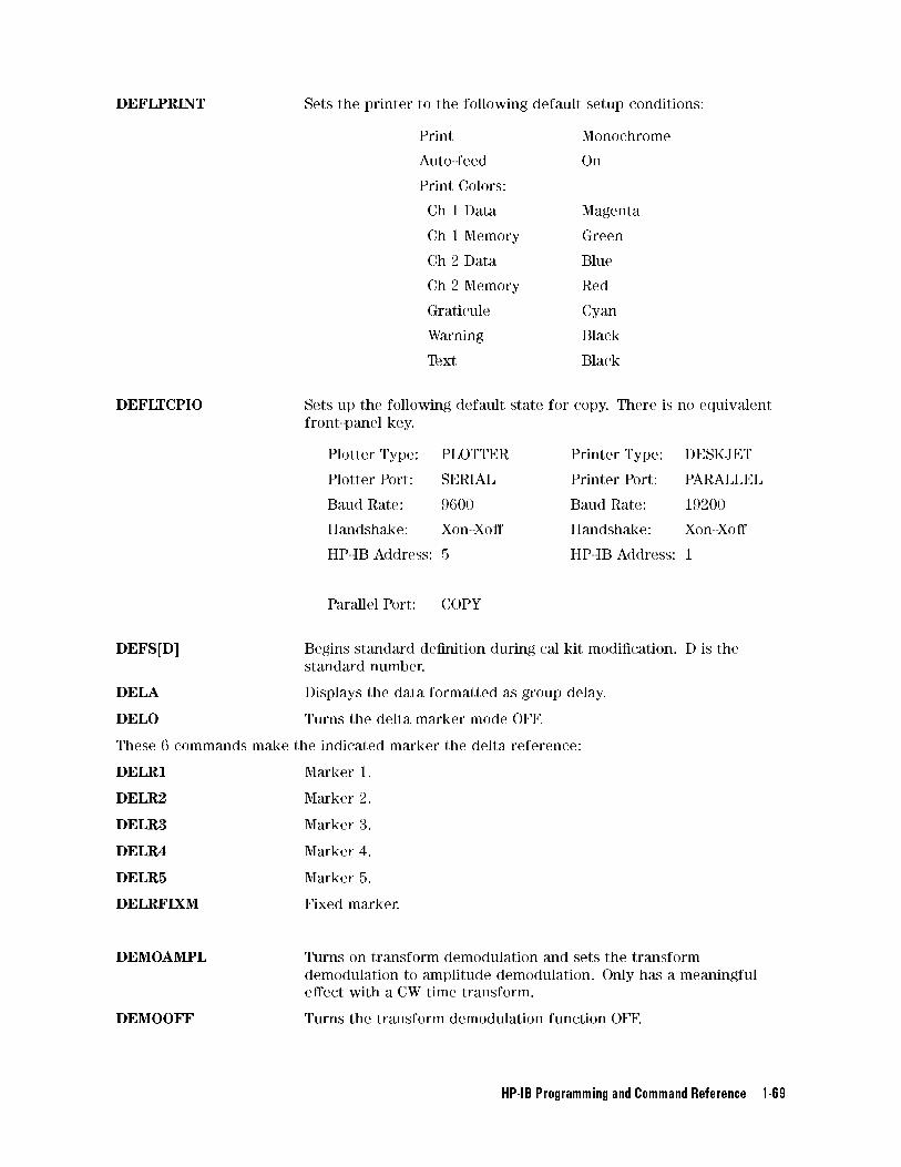
DEFLPRINT Sets the printer to the following default setup conditions:
Print Monochrome
Auto-feed On
Print Colors:
Ch 1 Data Magenta
Ch 1 Memory Green
Ch 2 Data Blue
Ch 2 Memory Red
Graticule Cyan
Warning Black
Text Black
DEFLTCPIO Sets up the following default state for copy. There is no equivalent
front-panel key.
Plotter Type: PLOTTER Printer Type: DESKJET
Plotter Port: SERIAL Printer Port: PARALLEL
Baud Rate: 9600 Baud Rate: 19200
Handshake: Xon-Xo� Handshake: Xon-Xo�
HP-IB Address: 5 HP-IB Address: 1
Parallel Port: COPY
DEFS[D] Begins standard de�nition during cal kit modi�cation. D is the
standard number.
DELA Displays the data formatted as group delay.
DELO Turns the delta marker mode OFF.
These 6 commands make the indicated marker the delta reference:
DELR1 Marker 1.
DELR2 Marker 2.
DELR3 Marker 3.
DELR4 Marker 4.
DELR5 Marker 5.
DELRFIXM Fixed marker.
DEMOAMPL Turns on transform demodulation and sets the transform
demodulation to amplitude demodulation. Only has a meaningful
e�ect with a CW time transform.
DEMOOFF Turns the transform demodulation function OFF.
HP-IB Programming and Command Reference 1-69
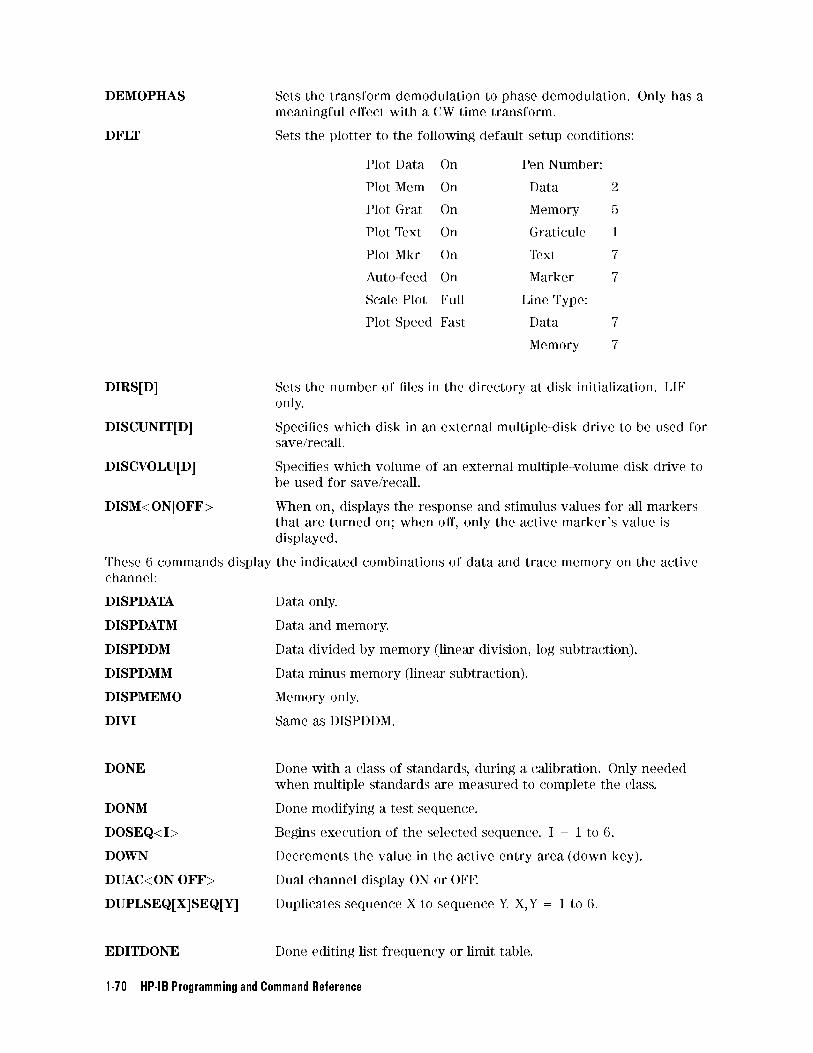
DEMOPHAS Sets the transform demodulation to phase demodulation. Only has a
meaningful e�ect with a CW time transform.
DFLT Sets the plotter to the following default setup conditions:
Plot Data On Pen Number:
Plot Mem On Data 2
Plot Grat On Memory 5
Plot Text On Graticule 1
Plot Mkr On Text 7
Auto-feed On Marker 7
Scale Plot Full Line Type:
Plot Speed Fast Data 7
Memory 7
DIRS[D] Sets the number of �les in the directory at disk initialization. LIF
only.
DISCUNIT[D] Speci�es which disk in an external multiple-disk drive to be used for
save/recall.
DISCVOLU[D] Speci�es which volume of an external multiple-volume disk drive to
be used for save/recall.
DISM<ONjOFF> When on, displays the response and stimulus values for all markers
that are turned on; when o�, only the active marker's value is
displayed.
These 6 commands display the indicated combinations of data and trace memory on the active
channel:
DISPDATA Data only.
DISPDATM Data and memory.
DISPDDM Data divided by memory (linear division, log subtraction).
DISPDMM Data minus memory (linear subtraction).
DISPMEMO Memory only.
DIVI Same as DISPDDM.
DONE Done with a class of standards, during a calibration. Only needed
when multiple standards are measured to complete the class.
DONM Done modifying a test sequence.
DOSEQ<I> Begins execution of the selected sequence. I = 1 to 6.
DOWN Decrements the value in the active entry area (down key).
DUAC<ONjOFF> Dual channel display ON or OFF.
DUPLSEQ[X]SEQ[Y] Duplicates sequence X to sequence Y. X,Y = 1 to 6.
EDITDONE Done editing list frequency or limit table.
1-70 HP-IB Programming and Command Reference
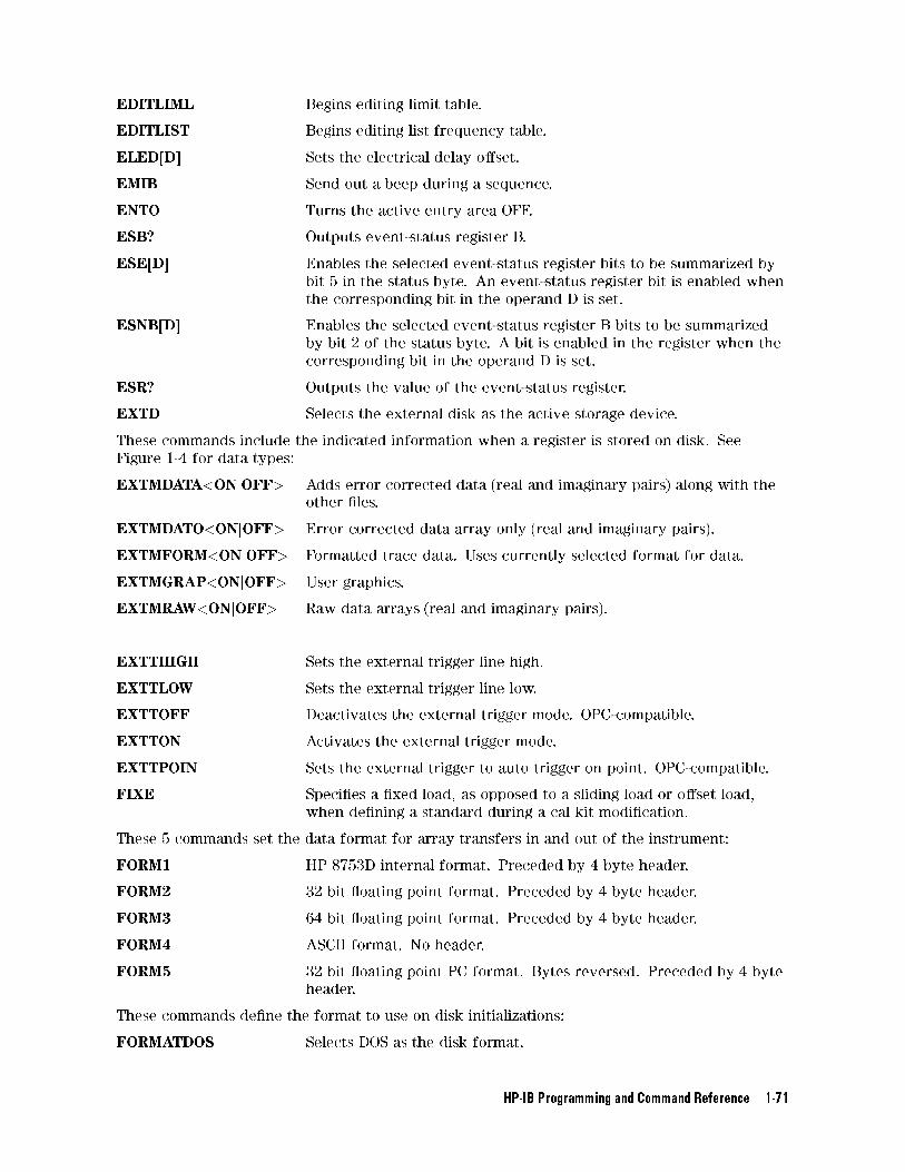
EDITLIML Begins editing limit table.
EDITLIST Begins editing list frequency table.
ELED[D] Sets the electrical delay o�set.
EMIB Send out a beep during a sequence.
ENTO Turns the active entry area OFF.
ESB? Outputs event-status register B.
ESE[D] Enables the selected event-status register bits to be summarized by
bit 5 in the status byte. An event-status register bit is enabled when
the corresponding bit in the operand D is set.
ESNB[D] Enables the selected event-status register B bits to be summarized
by bit 2 of the status byte. A bit is enabled in the register when the
corresponding bit in the operand D is set.
ESR? Outputs the value of the event-status register.
EXTD Selects the external disk as the active storage device.
These commands include the indicated information when a register is stored on disk. See
Figure 1-4 for data types:
EXTMDATA<ONjOFF> Adds error corrected data (real and imaginary pairs) along with the
other �les.
EXTMDATO<ONjOFF> Error corrected data array only (real and imaginary pairs).
EXTMFORM<ONjOFF> Formatted trace data. Uses currently selected format for data.
EXTMGRAP<ONjOFF> User graphics.
EXTMRAW<ONjOFF> Raw data arrays (real and imaginary pairs).
EXTTHIGH Sets the external trigger line high.
EXTTLOW Sets the external trigger line low.
EXTTOFF Deactivates the external trigger mode. OPC-compatible.
EXTTON Activates the external trigger mode.
EXTTPOIN Sets the external trigger to auto trigger on point. OPC-compatible.
FIXE Speci�es a �xed load, as opposed to a sliding load or o�set load,
when de�ning a standard during a cal kit modi�cation.
These 5 commands set the data format for array transfers in and out of the instrument:
FORM1 HP 8753D internal format. Preceded by 4 byte header.
FORM2 32 bit oating point format. Preceded by 4 byte header.
FORM3 64 bit oating point format. Preceded by 4 byte header.
FORM4 ASCII format. No header.
FORM5 32 bit oating point PC format. Bytes reversed. Preceded by 4 byte
header.
These commands de�ne the format to use on disk initializations:
FORMATDOS Selects DOS as the disk format.
HP-IB Programming and Command Reference 1-71
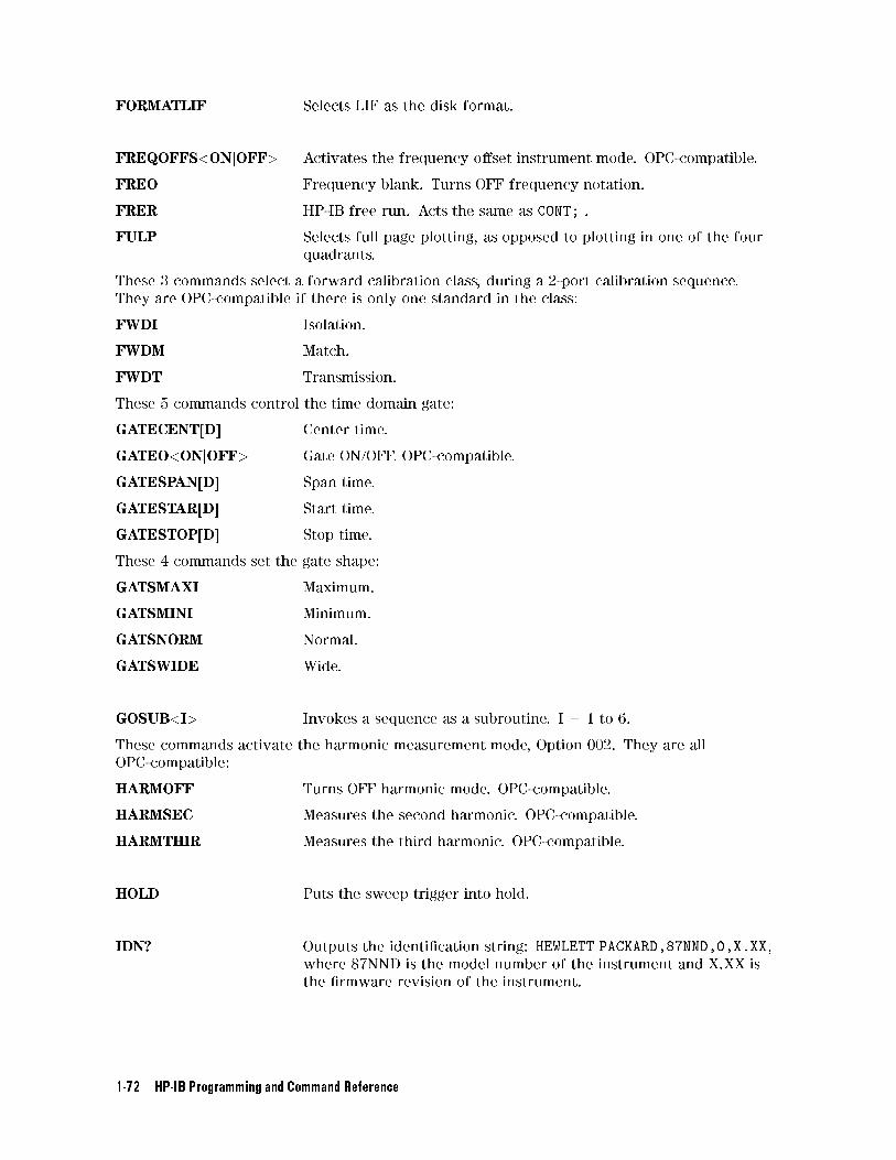
FORMATLIF Selects LIF as the disk format.
FREQOFFS<ONjOFF> Activates the frequency o�set instrument mode. OPC-compatible.
FREO Frequency blank. Turns OFF frequency notation.
FRER HP-IB free run. Acts the same as CONT; .
FULP Selects full page plotting, as opposed to plotting in one of the four
quadrants.
These 3 commands select a forward calibration class, during a 2-port calibration sequence.
They are OPC-compatible if there is only one standard in the class:
FWDI Isolation.
FWDM Match.
FWDT Transmission.
These 5 commands control the time domain gate:
GATECENT[D] Center time.
GATEO<ONjOFF> Gate ON/OFF. OPC-compatible.
GATESPAN[D] Span time.
GATESTAR[D] Start time.
GATESTOP[D] Stop time.
These 4 commands set the gate shape:
GATSMAXI Maximum.
GATSMINI Minimum.
GATSNORM Normal.
GATSWIDE Wide.
GOSUB<I> Invokes a sequence as a subroutine. I = 1 to 6.
These commands activate the harmonic measurement mode, Option 002. They are all
OPC-compatible:
HARMOFF Turns OFF harmonic mode. OPC-compatible.
HARMSEC Measures the second harmonic. OPC-compatible.
HARMTHIR Measures the third harmonic. OPC-compatible.
HOLD Puts the sweep trigger into hold.
IDN? Outputs the identi�cation string: HEWLETT PACKARD,87NND,0,X.XX,
where 87NND is the model number of the instrument and X.XX is
the �rmware revision of the instrument.
1-72 HP-IB Programming and Command Reference
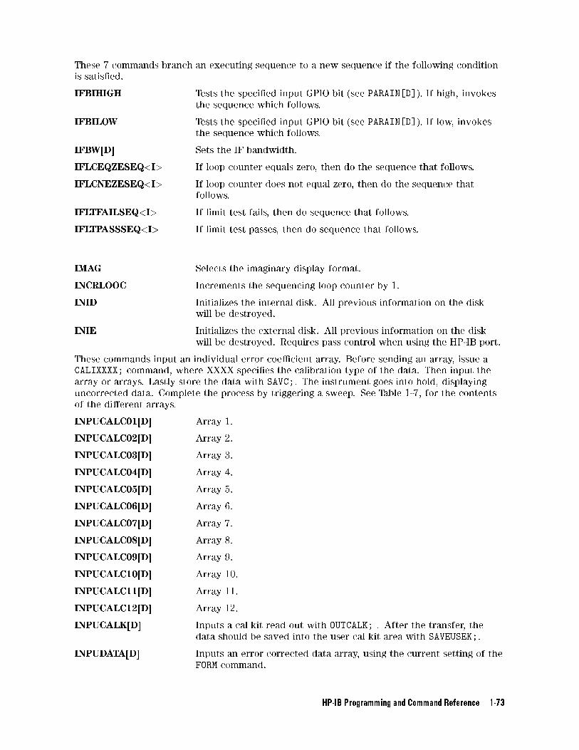
These 7 commands branch an executing sequence to a new sequence if the following condition
is satis�ed.
IFBIHIGH Tests the speci�ed input GPIO bit (see PARAIN[D]). If high, invokes
the sequence which follows.
IFBILOW Tests the speci�ed input GPIO bit (see PARAIN[D]). If low, invokes
the sequence which follows.
IFBW[D] Sets the IF bandwidth.
IFLCEQZESEQ<I> If loop counter equals zero, then do the sequence that follows.
IFLCNEZESEQ<I> If loop counter does not equal zero, then do the sequence that
follows.
IFLTFAILSEQ<I> If limit test fails, then do sequence that follows.
IFLTPASSSEQ<I> If limit test passes, then do sequence that follows.
IMAG Selects the imaginary display format.
INCRLOOC Increments the sequencing loop counter by 1.
INID Initializes the internal disk. All previous information on the disk
will be destroyed.
INIE Initializes the external disk. All previous information on the disk
will be destroyed. Requires pass control when using the HP-IB port.
These commands input an individual error coe�cient array. Before sending an array, issue a
CALIXXXX; command, where XXXX speci�es the calibration type of the data. Then input the
array or arrays. Lastly store the data with SAVC;. The instrument goes into hold, displaying
uncorrected data. Complete the process by triggering a sweep. See Table 1-7, for the contents
of the di�erent arrays.
INPUCALC01[D] Array 1.
INPUCALC02[D] Array 2.
INPUCALC03[D] Array 3.
INPUCALC04[D] Array 4.
INPUCALC05[D] Array 5.
INPUCALC06[D] Array 6.
INPUCALC07[D] Array 7.
INPUCALC08[D] Array 8.
INPUCALC09[D] Array 9.
INPUCALC10[D] Array 10.
INPUCALC11[D] Array 11.
INPUCALC12[D] Array 12.
INPUCALK[D] Inputs a cal kit read out with OUTCALK; . After the transfer, the
data should be saved into the user cal kit area with SAVEUSEK;.
INPUDATA[D] Inputs an error corrected data array, using the current setting of the
FORM command.
HP-IB Programming and Command Reference 1-73
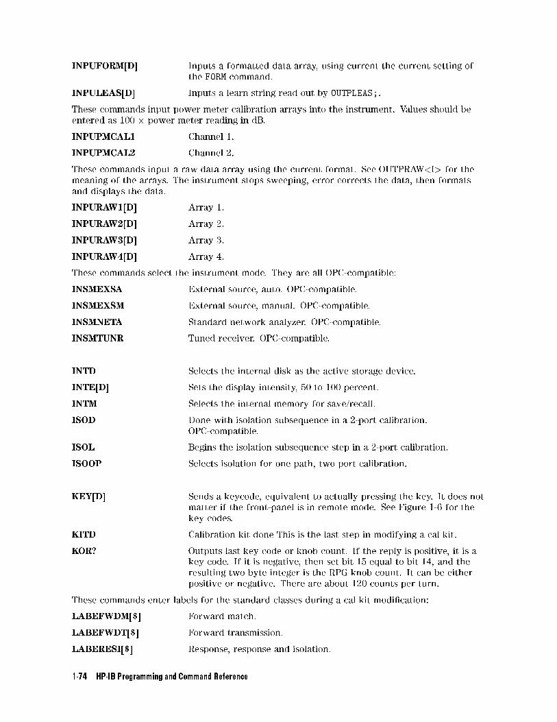
INPUFORM[D] Inputs a formatted data array, using current the current setting of
the FORM command.
INPULEAS[D] Inputs a learn string read out by OUTPLEAS;.
These commands input power meter calibration arrays into the instrument. Values should be
entered as 100 � power meter reading in dB.
INPUPMCAL1 Channel 1.
INPUPMCAL2 Channel 2.
These commands input a raw data array using the current format. See OUTPRAW<I> for the
meaning of the arrays. The instrument stops sweeping, error corrects the data, then formats
and displays the data.
INPURAW1[D] Array 1.
INPURAW2[D] Array 2.
INPURAW3[D] Array 3.
INPURAW4[D] Array 4.
These commands select the instrument mode. They are all OPC-compatible:
INSMEXSA External source, auto. OPC-compatible.
INSMEXSM External source, manual. OPC-compatible.
INSMNETA Standard network analyzer. OPC-compatible.
INSMTUNR Tuned receiver. OPC-compatible.
INTD Selects the internal disk as the active storage device.
INTE[D] Sets the display intensity, 50 to 100 percent.
INTM Selects the internal memory for save/recall.
ISOD Done with isolation subsequence in a 2-port calibration.
OPC-compatible.
ISOL Begins the isolation subsequence step in a 2-port calibration.
ISOOP Selects isolation for one path, two port calibration.
KEY[D] Sends a keycode, equivalent to actually pressing the key. It does not
matter if the front-panel is in remote mode. See Figure 1-6 for the
key codes.
KITD Calibration kit done This is the last step in modifying a cal kit.
KOR? Outputs last key code or knob count. If the reply is positive, it is a
key code. If it is negative, then set bit 15 equal to bit 14, and the
resulting two byte integer is the RPG knob count. It can be either
positive or negative. There are about 120 counts per turn.
These commands enter labels for the standard classes during a cal kit modi�cation:
LABEFWDM[$] Forward match.
LABEFWDT[$] Forward transmission.
LABERESI[$] Response, response and isolation.
1-74 HP-IB Programming and Command Reference
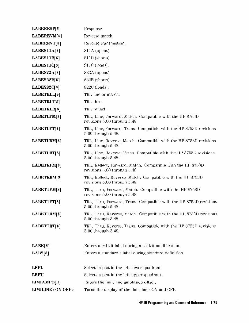
LABERESP[$] Response.
LABEREVM[$] Reverse match.
LABEREVT[$] Reverse transmission.
LABES11A[$] S11A (opens).
LABES11B[$] S11B (shorts).
LABES11C[$] S11C (loads).
LABES22A[$] S22A (opens).
LABES22B[$] S22B (shorts).
LABES22C[$] S22C (loads).
LABETRLL[$] TRL line or match.
LABETRLT[$] TRL thru.
LABETRLR[$] TRL re ect.
LABETLFM[$] TRL, Line, Forward, Match. Compatible with the HP 8753D
revisions 5.00 through 5.48.
LABETLFT[$] TRL, Line, Forward, Trans. Compatible with the HP 8753D revisions
5.00 through 5.48.
LABETLRM[$] TRL, Line, Reverse, Match. Compatible with the HP 8753D revisions
5.00 through 5.48.
LABETLRT[$] TRL, Line, Reverse, Trans. Compatible with the HP 8753D revisions
5.00 through 5.48.
LABETRFM[$] TRL, Re ect, Forward, Match. Compatible with the HP 8753D
revisions 5.00 through 5.48.
LABETRRM[$] TRL, Re ect, Reverse, Match. Compatible with the HP 8753D
revisions 5.00 through 5.48.
LABETTFM[$] TRL, Thru, Forward, Match. Compatible with the HP 8753D
revisions 5.00 through 5.48.
LABETTFT[$] TRL, Thru, Forward, Trans. Compatible with the HP 8753D revisions
5.00 through 5.48.
LABETTRM[$] TRL, Thru, Reverse, Match. Compatible with the HP 8753D revisions
5.00 through 5.48.
LABETTRT[$] TRL, Thru, Reverse, Trans. Compatible with the HP 8753D revisions
5.00 through 5.48.
LABK[$] Enters a cal kit label during a cal kit modi�cation.
LABS[$] Enters a standard's label during standard de�nition.
LEFL Selects a plot in the left lower quadrant.
LEFU Selects a plot in the left upper quadrant.
LIMIAMPO[D] Enters the limit line amplitude o�set.
LIMILINE<ONjOFF> Turns the display of the limit lines ON and OFF.
HP-IB Programming and Command Reference 1-75
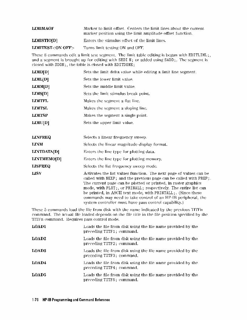
LIMIMAOF Marker to limit o�set. Centers the limit lines about the current
marker position using the limit amplitude o�set function.
LIMISTIO[D] Enters the stimulus o�set of the limit lines.
LIMITEST<ONjOFF> Turns limit testing ON and OFF.
These 8 commands edit a limit test segment. The limit table editing is begun with EDITLIML;,
and a segment is brought up for editing with SEDI N; or added using SADD;. The segment is
closed with SDON;, the table is closed with EDITDONE;
LIMD[D] Sets the limit delta value while editing a limit line segment.
LIML[D] Sets the lower limit value.
LIMM[D] Sets the middle limit value.
LIMS[D] Sets the limit stimulus break point.
LIMTFL Makes the segment a at line.
LIMTSL Makes the segment a sloping line.
LIMTSP Makes the segment a single point.
LIMU[D] Sets the upper limit value.
LINFREQ Selects a linear frequency sweep.
LINM Selects the linear magnitude display format.
LINTDATA[D] Enters the line type for plotting data.
LINTMEMO[D] Enters the line type for plotting memory.
LISFREQ Selects the list frequency sweep mode.
LISV Activates the list values function. The next page of values can be
called with NEXP; and the previous page can be called with PREP;.
The current page can be plotted or printed, in raster graphics
mode, with PLOT;, or PRINALL; respectively. The entire list can
be printed, in ASCII text mode, with PRINTALL;. (Since these
commands may need to take control of an HP-IB peripheral, the
system controller must have pass control capability.)
These 5 commands load the �le from disk with the name indicated by the previous TITFn
command. The actual �le loaded depends on the �le title in the �le position speci�ed by the
TITFn command. Requires pass control mode.
LOAD1 Loads the �le from disk using the �le name provided by the
preceding TITF1; command.
LOAD2 Loads the �le from disk using the �le name provided by the
preceding TITF2; command.
LOAD3 Loads the �le from disk using the �le name provided by the
preceding TITF3; command.
LOAD4 Loads the �le from disk using the �le name provided by the
preceding TITF4; command.
LOAD5 Loads the �le from disk using the �le name provided by the
preceding TITF5; command.
1-76 HP-IB Programming and Command Reference
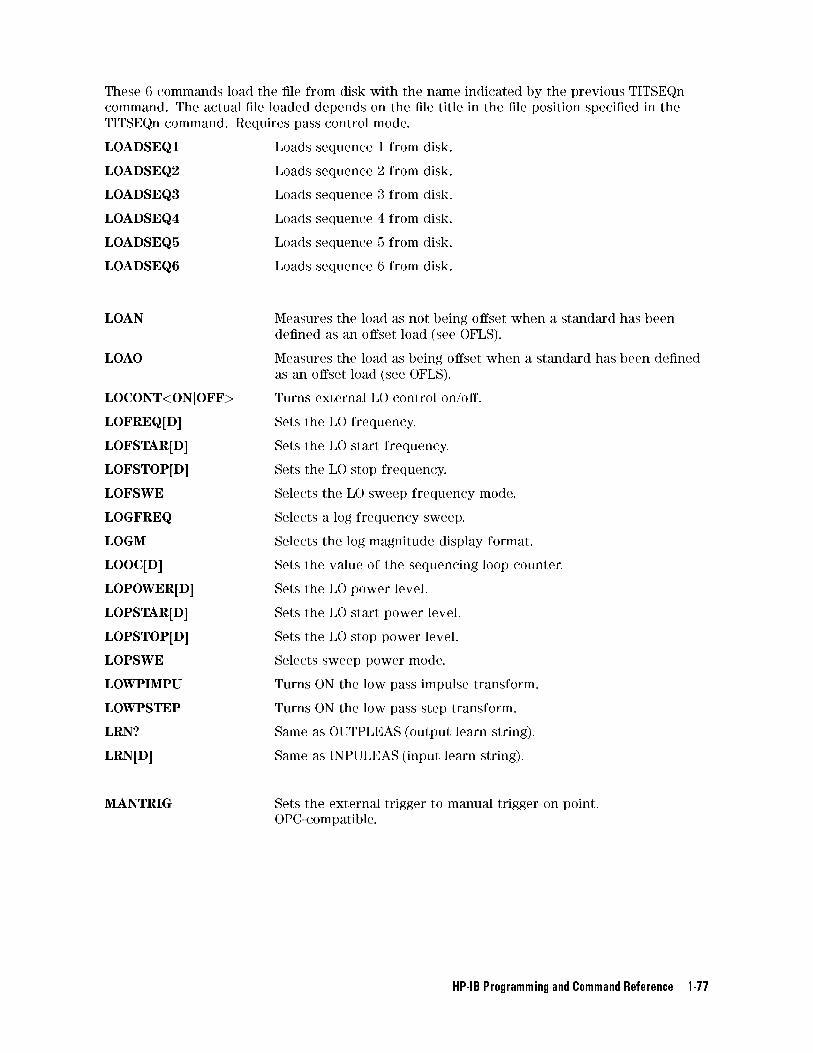
These 6 commands load the �le from disk with the name indicated by the previous TITSEQn
command. The actual �le loaded depends on the �le title in the �le position speci�ed in the
TITSEQn command. Requires pass control mode.
LOADSEQ1 Loads sequence 1 from disk.
LOADSEQ2 Loads sequence 2 from disk.
LOADSEQ3 Loads sequence 3 from disk.
LOADSEQ4 Loads sequence 4 from disk.
LOADSEQ5 Loads sequence 5 from disk.
LOADSEQ6 Loads sequence 6 from disk.
LOAN Measures the load as not being o�set when a standard has been
de�ned as an o�set load (see OFLS).
LOAO Measures the load as being o�set when a standard has been de�ned
as an o�set load (see OFLS).
LOCONT<ONjOFF> Turns external LO control on/o�.
LOFREQ[D] Sets the LO frequency.
LOFSTAR[D] Sets the LO start frequency.
LOFSTOP[D] Sets the LO stop frequency.
LOFSWE Selects the LO sweep frequency mode.
LOGFREQ Selects a log frequency sweep.
LOGM Selects the log magnitude display format.
LOOC[D] Sets the value of the sequencing loop counter.
LOPOWER[D] Sets the LO power level.
LOPSTAR[D] Sets the LO start power level.
LOPSTOP[D] Sets the LO stop power level.
LOPSWE Selects sweep power mode.
LOWPIMPU Turns ON the low pass impulse transform.
LOWPSTEP Turns ON the low pass step transform.
LRN? Same as OUTPLEAS (output learn string).
LRN[D] Same as INPULEAS (input learn string).
MANTRIG Sets the external trigger to manual trigger on point.
OPC-compatible.
HP-IB Programming and Command Reference 1-77
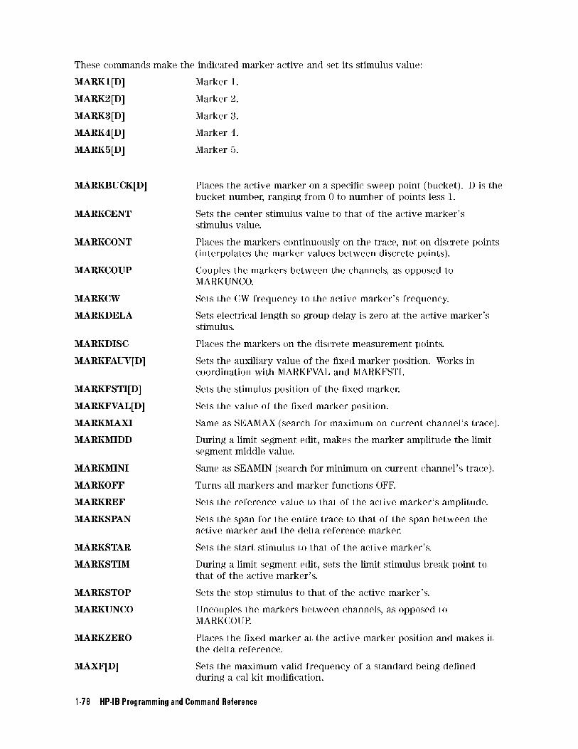
These commands make the indicated marker active and set its stimulus value:
MARK1[D] Marker 1.
MARK2[D] Marker 2.
MARK3[D] Marker 3.
MARK4[D] Marker 4.
MARK5[D] Marker 5.
MARKBUCK[D] Places the active marker on a speci�c sweep point (bucket). D is the
bucket number, ranging from 0 to number of points less 1.
MARKCENT Sets the center stimulus value to that of the active marker's
stimulus value.
MARKCONT Places the markers continuously on the trace, not on discrete points
(interpolates the marker values between discrete points).
MARKCOUP Couples the markers between the channels, as opposed to
MARKUNCO.
MARKCW Sets the CW frequency to the active marker's frequency.
MARKDELA Sets electrical length so group delay is zero at the active marker's
stimulus.
MARKDISC Places the markers on the discrete measurement points.
MARKFAUV[D] Sets the auxiliary value of the �xed marker position. Works in
coordination with MARKFVAL and MARKFSTI.
MARKFSTI[D] Sets the stimulus position of the �xed marker.
MARKFVAL[D] Sets the value of the �xed marker position.
MARKMAXI Same as SEAMAX (search for maximum on current channel's trace).
MARKMIDD During a limit segment edit, makes the marker amplitude the limit
segment middle value.
MARKMINI Same as SEAMIN (search for minimum on current channel's trace).
MARKOFF Turns all markers and marker functions OFF.
MARKREF Sets the reference value to that of the active marker's amplitude.
MARKSPAN Sets the span for the entire trace to that of the span between the
active marker and the delta reference marker.
MARKSTAR Sets the start stimulus to that of the active marker's.
MARKSTIM During a limit segment edit, sets the limit stimulus break point to
that of the active marker's.
MARKSTOP Sets the stop stimulus to that of the active marker's.
MARKUNCO Uncouples the markers between channels, as opposed to
MARKCOUP.
MARKZERO Places the �xed marker at the active marker position and makes it
the delta reference.
MAXF[D] Sets the maximum valid frequency of a standard being de�ned
during a cal kit modi�cation.
1-78 HP-IB Programming and Command Reference
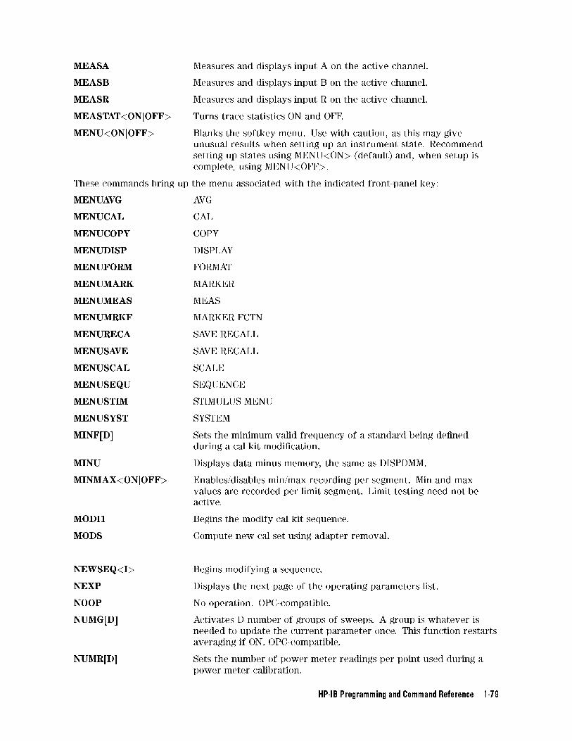
MEASA Measures and displays input A on the active channel.
MEASB Measures and displays input B on the active channel.
MEASR Measures and displays input R on the active channel.
MEASTAT<ONjOFF> Turns trace statistics ON and OFF.
MENU<ONjOFF> Blanks the softkey menu. Use with caution, as this may give
unusual results when setting up an instrument state. Recommend
setting up states using MENU<ON> (default) and, when setup is
complete, using MENU<OFF>.
These commands bring up the menu associated with the indicated front-panel key:
MENUAVG AVG
MENUCAL CAL
MENUCOPY COPY
MENUDISP DISPLAY
MENUFORM FORMAT
MENUMARK MARKER
MENUMEAS MEAS
MENUMRKF MARKER FCTN
MENURECA SAVE RECALL
MENUSAVE SAVE RECALL
MENUSCAL SCALE
MENUSEQU SEQUENCE
MENUSTIM STIMULUS MENU
MENUSYST SYSTEM
MINF[D] Sets the minimum valid frequency of a standard being de�ned
during a cal kit modi�cation.
MINU Displays data minus memory, the same as DISPDMM.
MINMAX<ONjOFF> Enables/disables min/max recording per segment. Min and max
values are recorded per limit segment. Limit testing need not be
active.
MODI1 Begins the modify cal kit sequence.
MODS Compute new cal set using adapter removal.
NEWSEQ<I> Begins modifying a sequence.
NEXP Displays the next page of the operating parameters list.
NOOP No operation. OPC-compatible.
NUMG[D] Activates D number of groups of sweeps. A group is whatever is
needed to update the current parameter once. This function restarts
averaging if ON. OPC-compatible.
NUMR[D] Sets the number of power meter readings per point used during a
power meter calibration.
HP-IB Programming and Command Reference 1-79
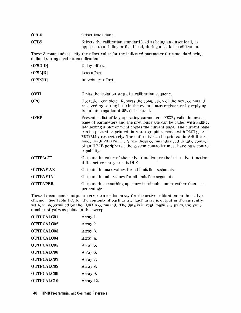
OFLD O�set loads done.
OFLS Selects the calibration standard load as being an o�set load, as
opposed to a sliding or �xed load, during a cal kit modi�cation.
These 3 commands specify the o�set value for the indicated parameter for a standard being
de�ned during a cal kit modi�cation:
OFSD[D] Delay o�set.
OFSL[D] Loss o�set.
OFSZ[D] Impedance o�set.
OMII Omits the isolation step of a calibration sequence.
OPC Operation complete. Reports the completion of the next command
received by setting bit 0 in the event-status register, or by replying
to an interrogation if OPC?; is issued.
OPEP Presents a list of key operating parameters. NEXP; calls the next
page of parameters and the previous page can be called with PREP;.
Requesting a plot or print copies the current page. The current page
can be plotted or printed, in raster graphics mode, with PLOT;, or
PRINALL; respectively. The entire list can be printed, in ASCII text
mode, with PRINTALL;. Since these commands need to take control
of an HP-IB peripheral, the system controller must have pass control
capability.
OUTPACTI Outputs the value of the active function, or the last active function
if the active entry area is OFF.
OUTPAMAX Outputs the max values for all limit line segments.
OUTPAMIN Outputs the min values for all limit line segments.
OUTPAPER Outputs the smoothing aperture in stimulus units, rather than as a
percentage.
These 12 commands output an error correction array for the active calibration on the active
channel. See Table 1-7, for the contents of each array. Each array is output in the currently
set form determined by the FORMn command. The data is in real/imaginary pairs, the same
number of pairs as points in the sweep.
OUTPCALC01 Array 1.
OUTPCALC02 Array 2.
OUTPCALC03 Array 3.
OUTPCALC04 Array 4.
OUTPCALC05 Array 5.
OUTPCALC06 Array 6.
OUTPCALC07 Array 7.
OUTPCALC08 Array 8.
OUTPCALC09 Array 9.
OUTPCALC10 Array 10.
1-80 HP-IB Programming and Command Reference
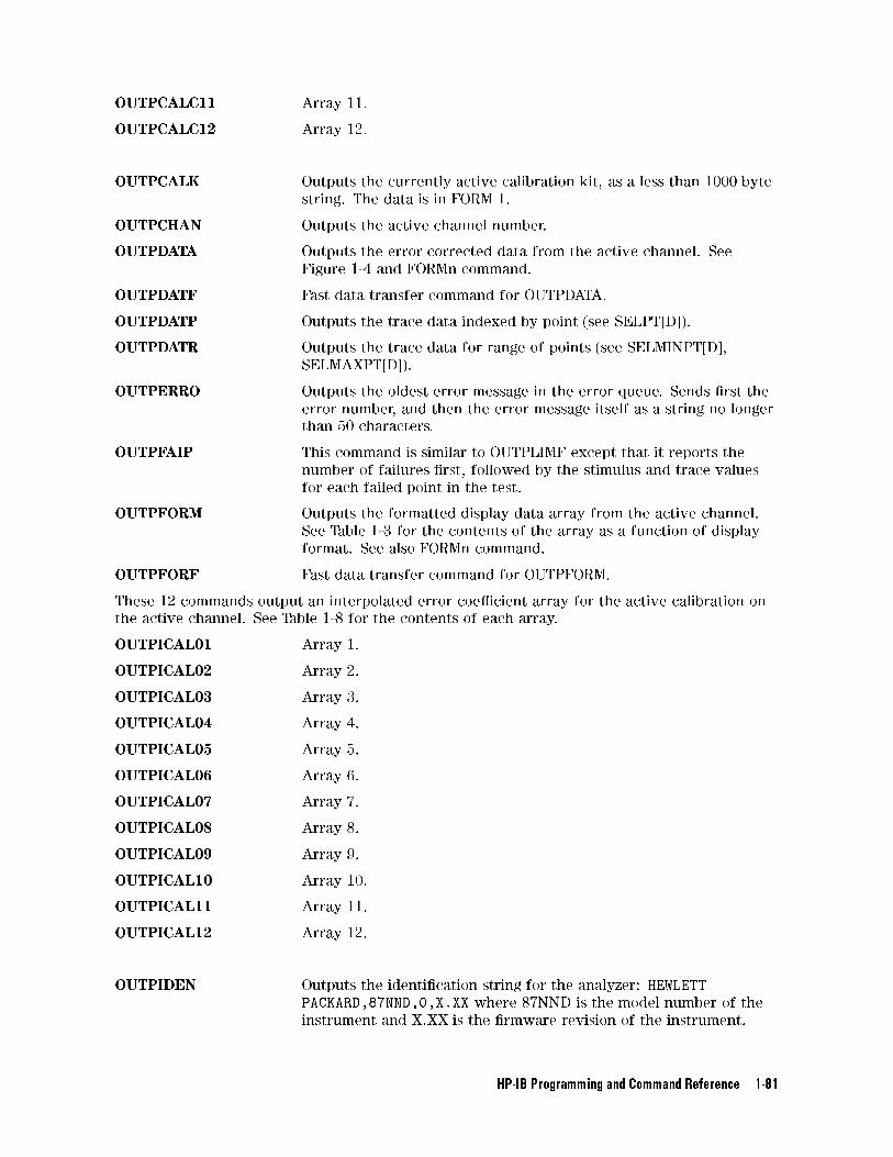
OUTPCALC11 Array 11.
OUTPCALC12 Array 12.
OUTPCALK Outputs the currently active calibration kit, as a less than 1000 byte
string. The data is in FORM 1.
OUTPCHAN Outputs the active channel number.
OUTPDATA Outputs the error corrected data from the active channel. See
Figure 1-4 and FORMn command.
OUTPDATF Fast data transfer command for OUTPDATA.
OUTPDATP Outputs the trace data indexed by point (see SELPT[D]).
OUTPDATR Outputs the trace data for range of points (see SELMINPT[D],
SELMAXPT[D]).
OUTPERRO Outputs the oldest error message in the error queue. Sends �rst the
error number, and then the error message itself as a string no longer
than 50 characters.
OUTPFAIP This command is similar to OUTPLIMF except that it reports the
number of failures �rst, followed by the stimulus and trace values
for each failed point in the test.
OUTPFORM Outputs the formatted display data array from the active channel.
See Table 1-3 for the contents of the array as a function of display
format. See also FORMn command.
OUTPFORF Fast data transfer command for OUTPFORM.
These 12 commands output an interpolated error coe�cient array for the active calibration on
the active channel. See Table 1-8 for the contents of each array.
OUTPICAL01 Array 1.
OUTPICAL02 Array 2.
OUTPICAL03 Array 3.
OUTPICAL04 Array 4.
OUTPICAL05 Array 5.
OUTPICAL06 Array 6.
OUTPICAL07 Array 7.
OUTPICAL08 Array 8.
OUTPICAL09 Array 9.
OUTPICAL10 Array 10.
OUTPICAL11 Array 11.
OUTPICAL12 Array 12.
OUTPIDEN Outputs the identi�cation string for the analyzer: HEWLETT
PACKARD,87NND,0,X.XX where 87NND is the model number of the
instrument and X.XX is the �rmware revision of the instrument.
HP-IB Programming and Command Reference 1-81
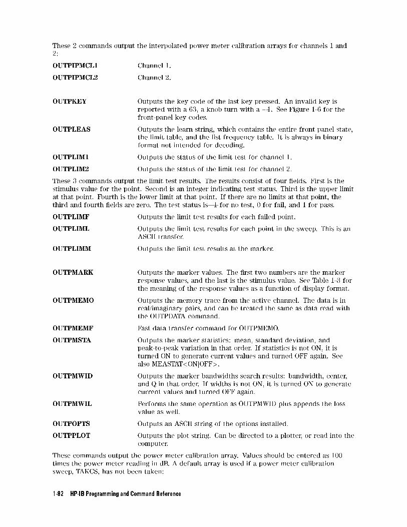
These 2 commands output the interpolated power meter calibration arrays for channels 1 and
2:
OUTPIPMCL1 Channel 1.
OUTPIPMCL2 Channel 2.
OUTPKEY Outputs the key code of the last key pressed. An invalid key is
reported with a 63, a knob turn with a �1. See Figure 1-6 for the
front-panel key codes.
OUTPLEAS Outputs the learn string, which contains the entire front panel state,
the limit table, and the list frequency table. It is always in binary
format not intended for decoding.
OUTPLIM1 Outputs the status of the limit test for channel 1.
OUTPLIM2 Outputs the status of the limit test for channel 2.
These 3 commands output the limit test results. The results consist of four �elds. First is the
stimulus value for the point. Second is an integer indicating test status. Third is the upper limit
at that point. Fourth is the lower limit at that point. If there are no limits at that point, the
third and fourth �elds are zero. The test status is|1 for no test, 0 for fail, and 1 for pass.
OUTPLIMF Outputs the limit test results for each failed point.
OUTPLIML Outputs the limit test results for each point in the sweep. This is an
ASCII transfer.
OUTPLIMM Outputs the limit test results at the marker.
OUTPMARK Outputs the marker values. The �rst two numbers are the marker
response values, and the last is the stimulus value. See Table 1-3 for
the meaning of the response values as a function of display format.
OUTPMEMO Outputs the memory trace from the active channel. The data is in
real/imaginary pairs, and can be treated the same as data read with
the OUTPDATA command.
OUTPMEMF Fast data transfer command for OUTPMEMO.
OUTPMSTA Outputs the marker statistics: mean, standard deviation, and
peak-to-peak variation in that order. If statistics is not ON, it is
turned ON to generate current values and turned OFF again. See
also MEASTAT<ONjOFF>.
OUTPMWID Outputs the marker bandwidths search results: bandwidth, center,
and Q in that order. If widths is not ON, it is turned ON to generate
current values and turned OFF again.
OUTPMWIL Performs the same operation as OUTPMWID plus appends the loss
value as well.
OUTPOPTS Outputs an ASCII string of the options installed.
OUTPPLOT Outputs the plot string. Can be directed to a plotter, or read into the
computer.
These commands output the power meter calibration array. Values should be entered as 100
times the power meter reading in dB. A default array is used if a power meter calibration
sweep, TAKCS, has not been taken:
1-82 HP-IB Programming and Command Reference
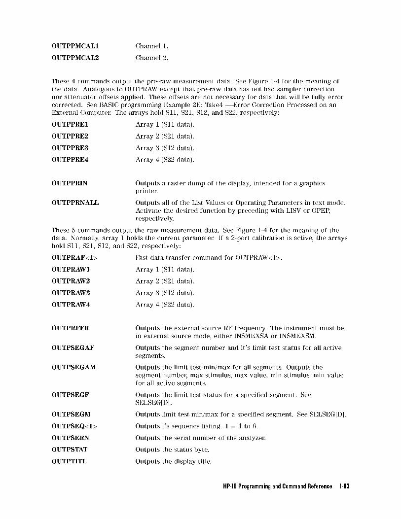
OUTPPMCAL1 Channel 1.
OUTPPMCAL2 Channel 2.
These 4 commands output the pre-raw measurement data. See Figure 1-4 for the meaning of
the data. Analogous to OUTPRAW except that pre-raw data has not had sampler correction
nor attenuator o�sets applied. These o�sets are not necessary for data that will be fully error
corrected. See BASIC programming Example 2E: Take4 | Error Correction Processed on an
External Computer. The arrays hold S11, S21, S12, and S22, respectively:
OUTPPRE1 Array 1 (S11 data).
OUTPPRE2 Array 2 (S21 data).
OUTPPRE3 Array 3 (S12 data).
OUTPPRE4 Array 4 (S22 data).
OUTPPRIN Outputs a raster dump of the display, intended for a graphics
printer.
OUTPPRNALL Outputs all of the List Values or Operating Parameters in text mode.
Activate the desired function by preceding with LISV or OPEP,
respectively.
These 5 commands output the raw measurement data. See Figure 1-4 for the meaning of the
data. Normally, array 1 holds the current parameter. If a 2-port calibration is active, the arrays
hold S11, S21, S12, and S22, respectively:
OUTPRAF<I> Fast data transfer command for OUTPRAW<I>.
OUTPRAW1 Array 1 (S11 data).
OUTPRAW2 Array 2 (S21 data).
OUTPRAW3 Array 3 (S12 data).
OUTPRAW4 Array 4 (S22 data).
OUTPRFFR Outputs the external source RF frequency. The instrument must be
in external source mode, either INSMEXSA or INSMEXSM.
OUTPSEGAF Outputs the segment number and it's limit test status for all active
segments.
OUTPSEGAM Outputs the limit test min/max for all segments. Outputs the
segment number, max stimulus, max value, min stimulus, min value
for all active segments.
OUTPSEGF Outputs the limit test status for a speci�ed segment. See
SELSEG[D].
OUTPSEGM Outputs limit test min/max for a speci�ed segment. See SELSEG[D].
OUTPSEQ<I> Outputs I's sequence listing. I = 1 to 6.
OUTPSERN Outputs the serial number of the analyzer.
OUTPSTAT Outputs the status byte.
OUTPTITL Outputs the display title.
HP-IB Programming and Command Reference 1-83
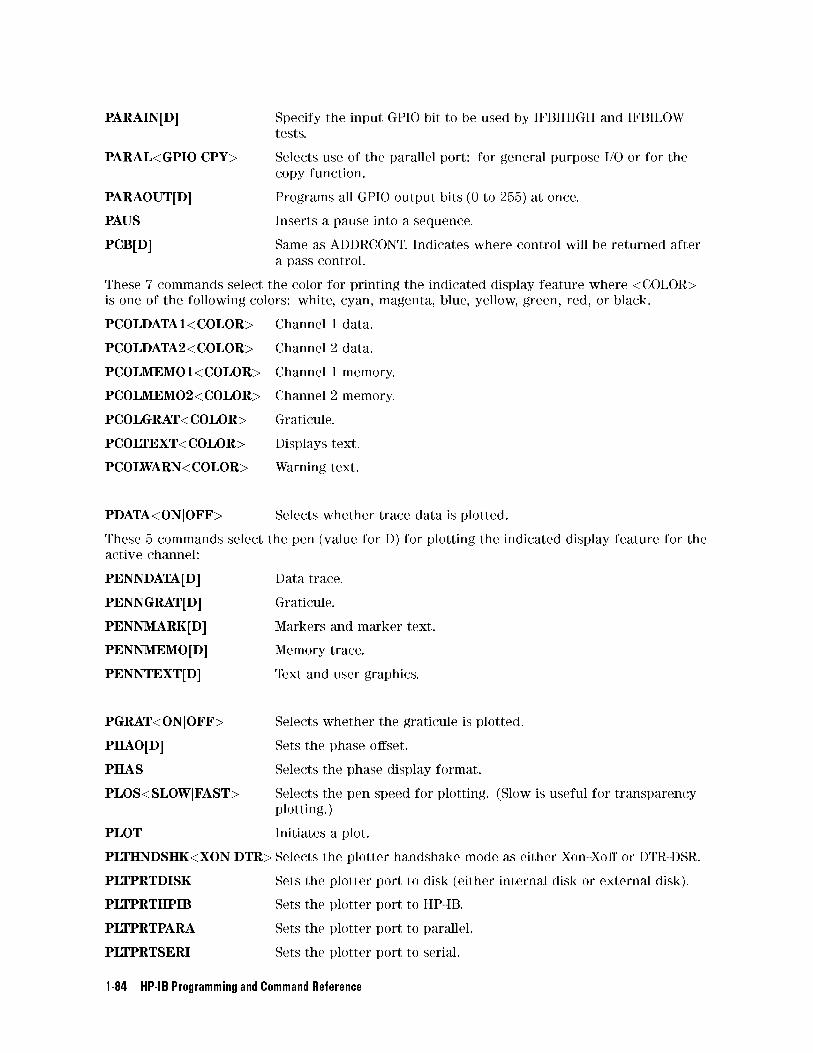
PARAIN[D] Specify the input GPIO bit to be used by IFBIHIGH and IFBILOW
tests.
PARAL<GPIOjCPY> Selects use of the parallel port: for general purpose I/O or for the
copy function.
PARAOUT[D] Programs all GPIO output bits (0 to 255) at once.
PAUS Inserts a pause into a sequence.
PCB[D] Same as ADDRCONT. Indicates where control will be returned after
a pass control.
These 7 commands select the color for printing the indicated display feature where <COLOR>
is one of the following colors: white, cyan, magenta, blue, yellow, green, red, or black.
PCOLDATA1<COLOR> Channel 1 data.
PCOLDATA2<COLOR> Channel 2 data.
PCOLMEMO1<COLOR> Channel 1 memory.
PCOLMEMO2<COLOR> Channel 2 memory.
PCOLGRAT<COLOR> Graticule.
PCOLTEXT<COLOR> Displays text.
PCOLWARN<COLOR> Warning text.
PDATA<ONjOFF> Selects whether trace data is plotted.
These 5 commands select the pen (value for D) for plotting the indicated display feature for the
active channel:
PENNDATA[D] Data trace.
PENNGRAT[D] Graticule.
PENNMARK[D] Markers and marker text.
PENNMEMO[D] Memory trace.
PENNTEXT[D] Text and user graphics.
PGRAT<ONjOFF> Selects whether the graticule is plotted.
PHAO[D] Sets the phase o�set.
PHAS Selects the phase display format.
PLOS<SLOWjFAST> Selects the pen speed for plotting. (Slow is useful for transparency
plotting.)
PLOT Initiates a plot.
PLTHNDSHK<XONjDTR>Selects the plotter handshake mode as either Xon-Xo� or DTR-DSR.
PLTPRTDISK Sets the plotter port to disk (either internal disk or external disk).
PLTPRTHPIB Sets the plotter port to HP-IB.
PLTPRTPARA Sets the plotter port to parallel.
PLTPRTSERI Sets the plotter port to serial.
1-84 HP-IB Programming and Command Reference
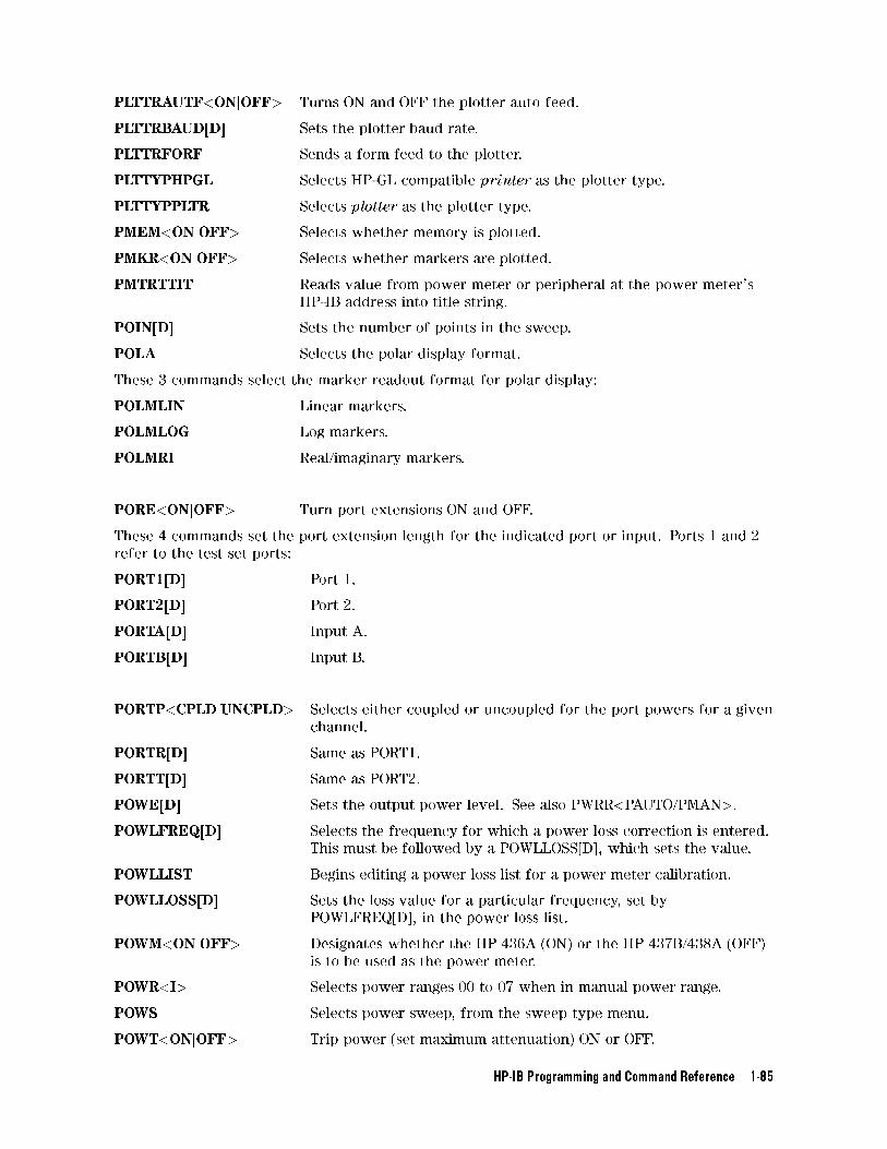
PLTTRAUTF<ONjOFF> Turns ON and OFF the plotter auto feed.
PLTTRBAUD[D] Sets the plotter baud rate.
PLTTRFORF Sends a form feed to the plotter.
PLTTYPHPGL Selects HP-GL compatible printer as the plotter type.
PLTTYPPLTR Selects plotter as the plotter type.
PMEM<ONjOFF> Selects whether memory is plotted.
PMKR<ONjOFF> Selects whether markers are plotted.
PMTRTTIT Reads value from power meter or peripheral at the power meter's
HP-IB address into title string.
POIN[D] Sets the number of points in the sweep.
POLA Selects the polar display format.
These 3 commands select the marker readout format for polar display:
POLMLIN Linear markers.
POLMLOG Log markers.
POLMRI Real/imaginary markers.
PORE<ONjOFF> Turn port extensions ON and OFF.
These 4 commands set the port extension length for the indicated port or input. Ports 1 and 2
refer to the test set ports:
PORT1[D] Port 1.
PORT2[D] Port 2.
PORTA[D] Input A.
PORTB[D] Input B.
PORTP<CPLDjUNCPLD> Selects either coupled or uncoupled for the port powers for a given
channel.
PORTR[D] Same as PORT1.
PORTT[D] Same as PORT2.
POWE[D] Sets the output power level. See also PWRR<PAUTO/PMAN>.
POWLFREQ[D] Selects the frequency for which a power loss correction is entered.
This must be followed by a POWLLOSS[D], which sets the value.
POWLLIST Begins editing a power loss list for a power meter calibration.
POWLLOSS[D] Sets the loss value for a particular frequency, set by
POWLFREQ[D], in the power loss list.
POWM<ONjOFF> Designates whether the HP 436A (ON) or the HP 437B/438A (OFF)
is to be used as the power meter.
POWR<I> Selects power ranges 00 to 07 when in manual power range.
POWS Selects power sweep, from the sweep type menu.
POWT<ONjOFF> Trip power (set maximum attenuation) ON or OFF.
HP-IB Programming and Command Reference 1-85
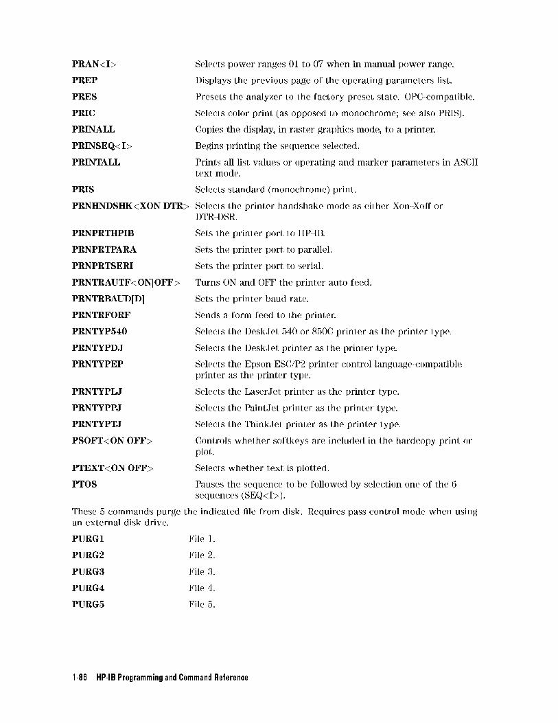
PRAN<I> Selects power ranges 01 to 07 when in manual power range.
PREP Displays the previous page of the operating parameters list.
PRES Presets the analyzer to the factory preset state. OPC-compatible.
PRIC Selects color print (as opposed to monochrome; see also PRIS).
PRINALL Copies the display, in raster graphics mode, to a printer.
PRINSEQ<I> Begins printing the sequence selected.
PRINTALL Prints all list values or operating and marker parameters in ASCII
text mode.
PRIS Selects standard (monochrome) print.
PRNHNDSHK<XONjDTR> Selects the printer handshake mode as either Xon-Xo� or
DTR-DSR.
PRNPRTHPIB Sets the printer port to HP-IB.
PRNPRTPARA Sets the printer port to parallel.
PRNPRTSERI Sets the printer port to serial.
PRNTRAUTF<ONjOFF> Turns ON and OFF the printer auto feed.
PRNTRBAUD[D] Sets the printer baud rate.
PRNTRFORF Sends a form feed to the printer.
PRNTYP540 Selects the DeskJet 540 or 850C printer as the printer type.
PRNTYPDJ Selects the DeskJet printer as the printer type.
PRNTYPEP Selects the Epson ESC/P2 printer control language-compatible
printer as the printer type.
PRNTYPLJ Selects the LaserJet printer as the printer type.
PRNTYPPJ Selects the PaintJet printer as the printer type.
PRNTYPTJ Selects the ThinkJet printer as the printer type.
PSOFT<ONjOFF> Controls whether softkeys are included in the hardcopy print or
plot.
PTEXT<ONjOFF> Selects whether text is plotted.
PTOS Pauses the sequence to be followed by selection one of the 6
sequences (SEQ<I>).
These 5 commands purge the indicated �le from disk. Requires pass control mode when using
an external disk drive.
PURG1 File 1.
PURG2 File 2.
PURG3 File 3.
PURG4 File 4.
PURG5 File 5.
1-86 HP-IB Programming and Command Reference
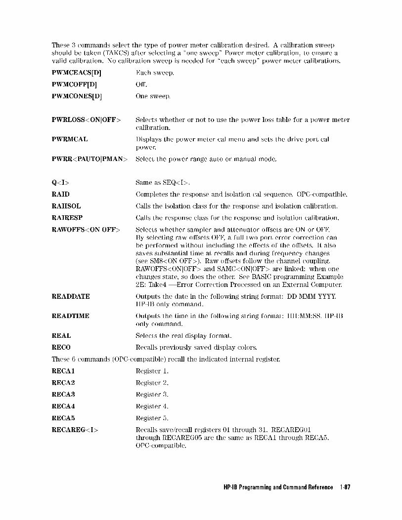
These 3 commands select the type of power meter calibration desired. A calibration sweep
should be taken (TAKCS) after selecting a \one sweep" Power meter calibration, to ensure a
valid calibration. No calibration sweep is needed for \each sweep" power meter calibrations.
PWMCEACS[D] Each sweep.
PWMCOFF[D] O�.
PWMCONES[D] One sweep.
PWRLOSS<ONjOFF> Selects whether or not to use the power loss table for a power meter
calibration.
PWRMCAL Displays the power meter cal menu and sets the drive port cal
power.
PWRR<PAUTOjPMAN> Select the power range auto or manual mode.
Q<I> Same as SEQ<I>.
RAID Completes the response and isolation cal sequence. OPC-compatible.
RAIISOL Calls the isolation class for the response and isolation calibration.
RAIRESP Calls the response class for the response and isolation calibration.
RAWOFFS<ONjOFF> Selects whether sampler and attenuator o�sets are ON or OFF.
By selecting raw o�sets OFF, a full two port error correction can
be performed without including the e�ects of the o�sets. It also
saves substantial time at recalls and during frequency changes
(see SM8<ONjOFF>). Raw o�sets follow the channel coupling.
RAWOFFS<ONjOFF> and SAMC<ONjOFF> are linked: when one
changes state, so does the other. See BASIC programming Example
2E: Take4 | Error Correction Processed on an External Computer.
READDATE Outputs the date in the following string format: DD MMM YYYY.
HP-IB only command.
READTIME Outputs the time in the following string format: HH:MM:SS. HP-IB
only command.
REAL Selects the real display format.
RECO Recalls previously saved display colors.
These 6 commands (OPC-compatible) recall the indicated internal register.
RECA1 Register 1.
RECA2 Register 2.
RECA3 Register 3.
RECA4 Register 4.
RECA5 Register 5.
RECAREG<I> Recalls save/recall registers 01 through 31. RECAREG01
through RECAREG05 are the same as RECA1 through RECA5.
OPC-compatible.
HP-IB Programming and Command Reference 1-87
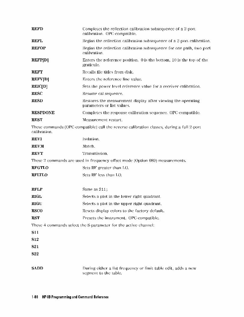
REFD Completes the re ection calibration subsequence of a 2-port
calibration. OPC-compatible.
REFL Begins the re ection calibration subsequence of a 2-port calibration.
REFOP Begins the re ection calibration subsequence for one path, two port
calibration.
REFP[D] Enters the reference position. 0 is the bottom, 10 is the top of the
graticule.
REFT Recalls �le titles from disk.
REFV[D] Enters the reference line value.
REIC[D] Sets the power level reference value for a receiver calibration.
RESC Resume cal sequence.
RESD Restores the measurement display after viewing the operating
parameters or list values.
RESPDONE Completes the response calibration sequence. OPC-compatible.
REST Measurement restart.
These commands (OPC-compatible) call the reverse calibration classes, during a full 2-port
calibration.
REVI Isolation.
REVM Match.
REVT Transmission.
These 2 commands are used in frequency o�set mode (Option 089) measurements.
RFGTLO Sets RF greater than LO.
RFLTLO Sets RF less than LO.
RFLP Same as S11;
RIGL Selects a plot in the lower right quadrant.
RIGU Selects a plot in the upper right quadrant.
RSCO Resets display colors to the factory default.
RST Presets the instrument. OPC-compatible.
These 4 commands select the S-parameter for the active channel:
S11
S12
S21
S22
SADD During either a list frequency or limit table edit, adds a new
segment to the table.
1-88 HP-IB Programming and Command Reference
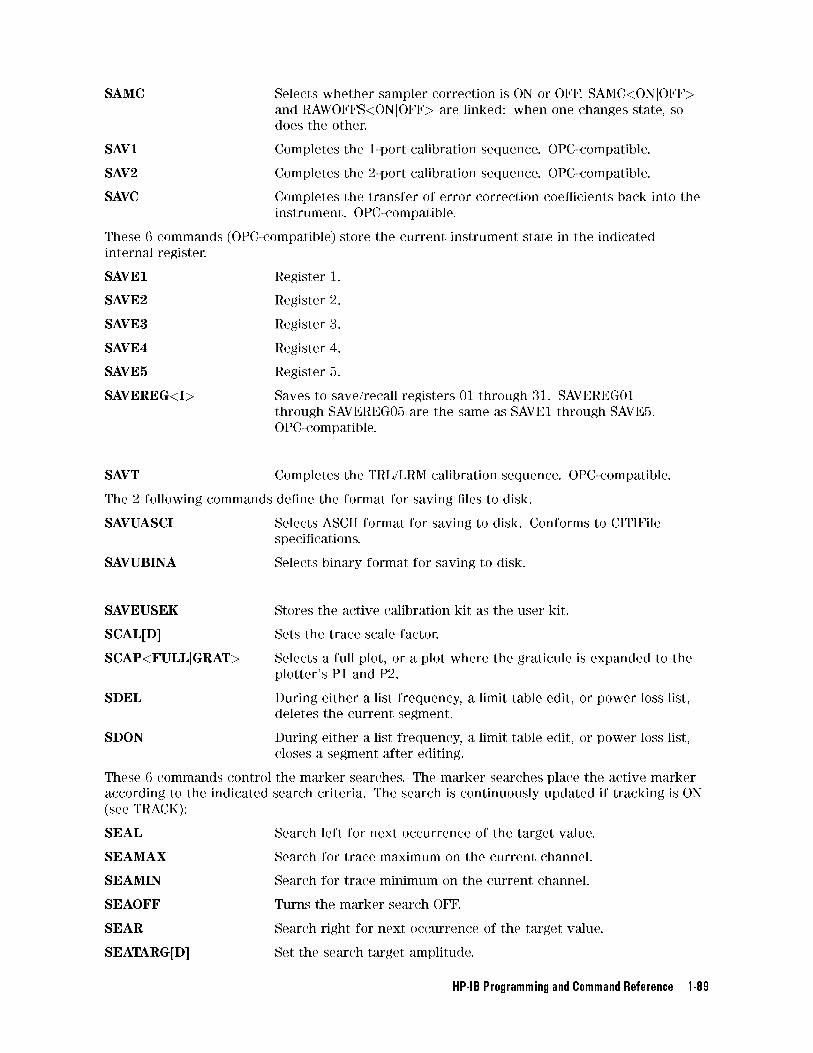
SAMC Selects whether sampler correction is ON or OFF. SAMC<ONjOFF>and RAWOFFS<ONjOFF> are linked: when one changes state, so
does the other.
SAV1 Completes the 1-port calibration sequence. OPC-compatible.
SAV2 Completes the 2-port calibration sequence. OPC-compatible.
SAVC Completes the transfer of error correction coe�cients back into the
instrument. OPC-compatible.
These 6 commands (OPC-compatible) store the current instrument state in the indicated
internal register.
SAVE1 Register 1.
SAVE2 Register 2.
SAVE3 Register 3.
SAVE4 Register 4.
SAVE5 Register 5.
SAVEREG<I> Saves to save/recall registers 01 through 31. SAVEREG01
through SAVEREG05 are the same as SAVE1 through SAVE5.
OPC-compatible.
SAVT Completes the TRL/LRM calibration sequence. OPC-compatible.
The 2 following commands de�ne the format for saving �les to disk.
SAVUASCI Selects ASCII format for saving to disk. Conforms to CITIFile
speci�cations.
SAVUBINA Selects binary format for saving to disk.
SAVEUSEK Stores the active calibration kit as the user kit.
SCAL[D] Sets the trace scale factor.
SCAP<FULLjGRAT> Selects a full plot, or a plot where the graticule is expanded to the
plotter's P1 and P2.
SDEL During either a list frequency, a limit table edit, or power loss list,
deletes the current segment.
SDON During either a list frequency, a limit table edit, or power loss list,
closes a segment after editing.
These 6 commands control the marker searches. The marker searches place the active marker
according to the indicated search criteria. The search is continuously updated if tracking is ON
(see TRACK):
SEAL Search left for next occurrence of the target value.
SEAMAX Search for trace maximum on the current channel.
SEAMIN Search for trace minimum on the current channel.
SEAOFF Turns the marker search OFF.
SEAR Search right for next occurrence of the target value.
SEATARG[D] Set the search target amplitude.
HP-IB Programming and Command Reference 1-89
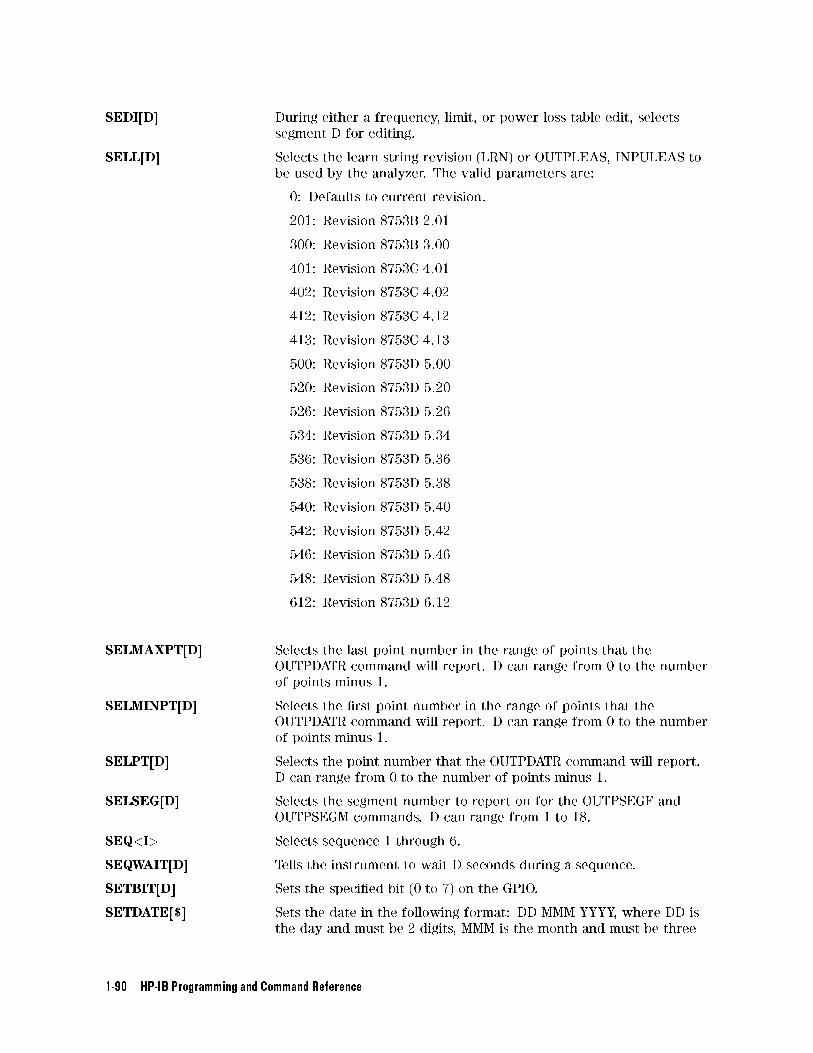
SEDI[D] During either a frequency, limit, or power loss table edit, selects
segment D for editing.
SELL[D] Selects the learn string revision (LRN) or OUTPLEAS, INPULEAS to
be used by the analyzer. The valid parameters are:
0: Defaults to current revision.
201: Revision 8753B 2.01
300: Revision 8753B 3.00
401: Revision 8753C 4.01
402: Revision 8753C 4.02
412: Revision 8753C 4.12
413: Revision 8753C 4.13
500: Revision 8753D 5.00
520: Revision 8753D 5.20
526: Revision 8753D 5.26
534: Revision 8753D 5.34
536: Revision 8753D 5.36
538: Revision 8753D 5.38
540: Revision 8753D 5.40
542: Revision 8753D 5.42
546: Revision 8753D 5.46
548: Revision 8753D 5.48
612: Revision 8753D 6.12
SELMAXPT[D] Selects the last point number in the range of points that the
OUTPDATR command will report. D can range from 0 to the number
of points minus 1.
SELMINPT[D] Selects the �rst point number in the range of points that the
OUTPDATR command will report. D can range from 0 to the number
of points minus 1.
SELPT[D] Selects the point number that the OUTPDATR command will report.
D can range from 0 to the number of points minus 1.
SELSEG[D] Selects the segment number to report on for the OUTPSEGF and
OUTPSEGM commands. D can range from 1 to 18.
SEQ<I> Selects sequence 1 through 6.
SEQWAIT[D] Tells the instrument to wait D seconds during a sequence.
SETBIT[D] Sets the speci�ed bit (0 to 7) on the GPIO.
SETDATE[$] Sets the date in the following format: DD MMM YYYY, where DD is
the day and must be 2 digits, MMM is the month and must be three
1-90 HP-IB Programming and Command Reference
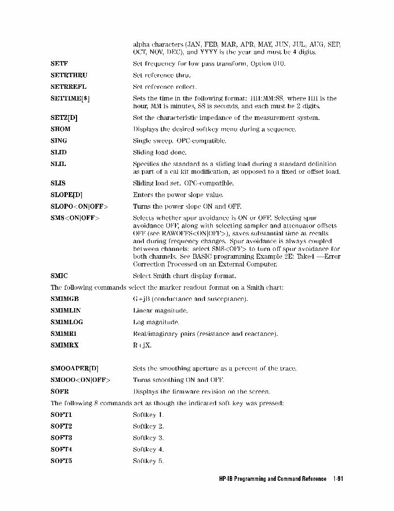
alpha characters (JAN, FEB, MAR, APR, MAY, JUN, JUL, AUG, SEP,
OCT, NOV, DEC), and YYYY is the year and must be 4 digits.
SETF Set frequency for low pass transform, Option 010.
SETRTHRU Set reference thru.
SETRREFL Set reference re ect.
SETTIME[$] Sets the time in the following format: HH:MM:SS, where HH is the
hour, MM is minutes, SS is seconds, and each must be 2 digits.
SETZ[D] Set the characteristic impedance of the measurement system.
SHOM Displays the desired softkey menu during a sequence.
SING Single sweep. OPC-compatible.
SLID Sliding load done.
SLIL Speci�es the standard as a sliding load during a standard de�nition
as part of a cal kit modi�cation, as opposed to a �xed or o�set load.
SLIS Sliding load set. OPC-compatible.
SLOPE[D] Enters the power slope value.
SLOPO<ONjOFF> Turns the power slope ON and OFF.
SM8<ONjOFF> Selects whether spur avoidance is ON or OFF. Selecting spur
avoidance OFF, along with selecting sampler and attenuator o�sets
OFF (see RAWOFFS<ONjOFF>), saves substantial time at recallsand during frequency changes. Spur avoidance is always coupled
between channels: select SM8<OFF> to turn o� spur avoidance for
both channels. See BASIC programming Example 2E: Take4 | Error
Correction Processed on an External Computer.
SMIC Select Smith chart display format.
The following commands select the marker readout format on a Smith chart:
SMIMGB G+jB (conductance and susceptance).
SMIMLIN Linear magnitude.
SMIMLOG Log magnitude.
SMIMRI Real/imaginary pairs (resistance and reactance).
SMIMRX R+jX.
SMOOAPER[D] Sets the smoothing aperture as a percent of the trace.
SMOOO<ONjOFF> Turns smoothing ON and OFF.
SOFR Displays the �rmware revision on the screen.
The following 8 commands act as though the indicated soft key was pressed:
SOFT1 Softkey 1.
SOFT2 Softkey 2.
SOFT3 Softkey 3.
SOFT4 Softkey 4.
SOFT5 Softkey 5.
HP-IB Programming and Command Reference 1-91
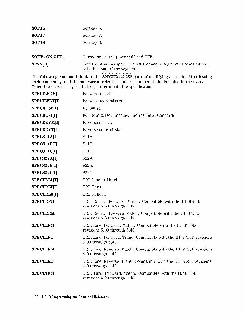
SOFT6 Softkey 6.
SOFT7 Softkey 7.
SOFT8 Softkey 8.
SOUP<ONjOFF> Turns the source power ON and OFF.
SPAN[D] Sets the stimulus span. If a list frequency segment is being edited,
sets the span of the segment.
The following commands initiate theNNNNNNNNNNNNNNNNNNNNNNNNNNNNNNNNNNNNNNNNNSPECIFY CLASS part of modifying a cal kit. After issuing
each command, send the analyzer a series of standard numbers to be included in the class.
When the class is full, send CLAD; to terminate the speci�cation.
SPECFWDM[I] Forward match.
SPECFWDT[I] Forward transmission.
SPECRESP[I] Response.
SPECRESI[I] For Resp & Isol, speci�es the response standards.
SPECREVM[I] Reverse match.
SPECREVT[I] Reverse transmission.
SPECS11A[I] S11A.
SPECS11B[I] S11B.
SPECS11C[I] S11C.
SPECS22A[I] S22A.
SPECS22B[I] S22B.
SPECS22C[I] S22C.
SPECTRLL[I] TRL Line or Match.
SPECTRLT[I] TRL Thru.
SPECTRLR[I] TRL Re ect.
SPECTRFM TRL, Re ect, Forward, Match. Compatible with the HP 8753D
revisions 5.00 through 5.48.
SPECTRRM TRL, Re ect, Reverse, Match. Compatible with the HP 8753D
revisions 5.00 through 5.48.
SPECTLFM TRL, Line, Forward, Match. Compatible with the HP 8753D
revisions 5.00 through 5.48.
SPECTLFT TRL, Line, Forward, Trans. Compatible with the HP 8753D revisions
5.00 through 5.48.
SPECTLRM TRL, Line, Reverse, Match. Compatible with the HP 8753D revisions
5.00 through 5.48.
SPECTLRT TRL, Line, Reverse, Trans. Compatible with the HP 8753D revisions
5.00 through 5.48.
SPECTTFM TRL, Thru, Forward, Match. Compatible with the HP 8753D
revisions 5.00 through 5.48.
1-92 HP-IB Programming and Command Reference
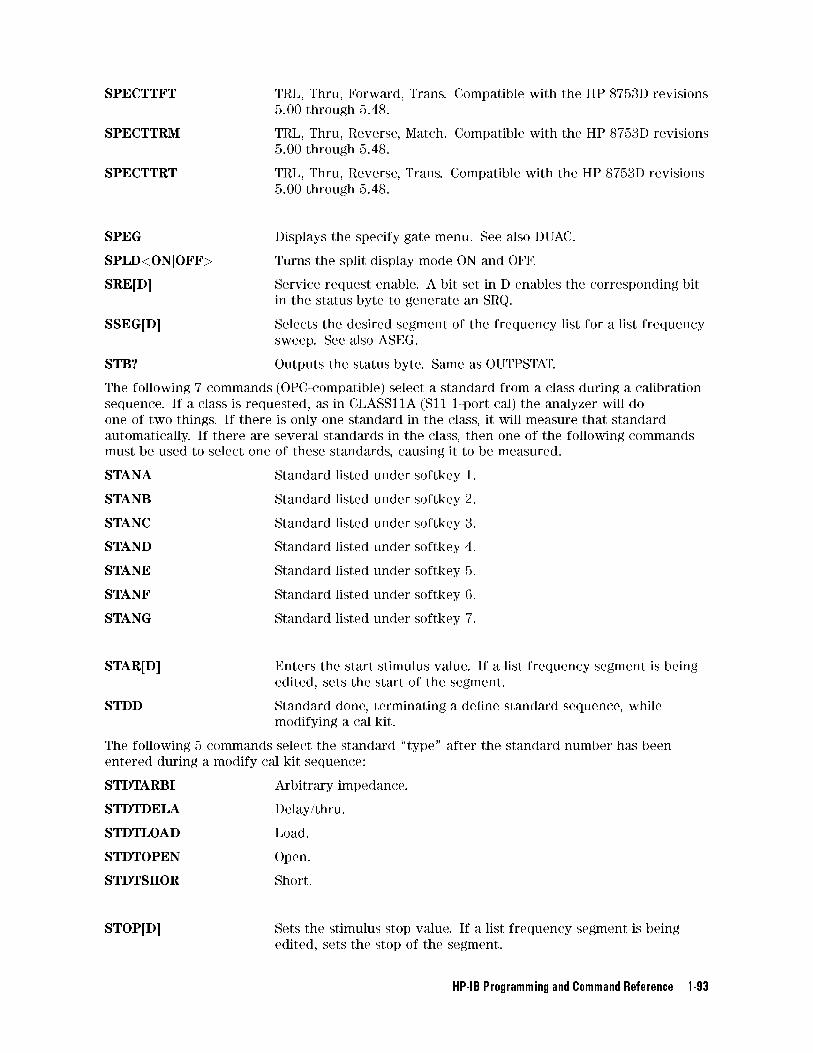
SPECTTFT TRL, Thru, Forward, Trans. Compatible with the HP 8753D revisions
5.00 through 5.48.
SPECTTRM TRL, Thru, Reverse, Match. Compatible with the HP 8753D revisions
5.00 through 5.48.
SPECTTRT TRL, Thru, Reverse, Trans. Compatible with the HP 8753D revisions
5.00 through 5.48.
SPEG Displays the specify gate menu. See also DUAC.
SPLD<ONjOFF> Turns the split display mode ON and OFF.
SRE[D] Service request enable. A bit set in D enables the corresponding bit
in the status byte to generate an SRQ.
SSEG[D] Selects the desired segment of the frequency list for a list frequency
sweep. See also ASEG.
STB? Outputs the status byte. Same as OUTPSTAT.
The following 7 commands (OPC-compatible) select a standard from a class during a calibration
sequence. If a class is requested, as in CLASS11A (S11 1-port cal) the analyzer will do
one of two things. If there is only one standard in the class, it will measure that standard
automatically. If there are several standards in the class, then one of the following commands
must be used to select one of these standards, causing it to be measured.
STANA Standard listed under softkey 1.
STANB Standard listed under softkey 2.
STANC Standard listed under softkey 3.
STAND Standard listed under softkey 4.
STANE Standard listed under softkey 5.
STANF Standard listed under softkey 6.
STANG Standard listed under softkey 7.
STAR[D] Enters the start stimulus value. If a list frequency segment is being
edited, sets the start of the segment.
STDD Standard done, terminating a de�ne standard sequence, while
modifying a cal kit.
The following 5 commands select the standard \type" after the standard number has been
entered during a modify cal kit sequence:
STDTARBI Arbitrary impedance.
STDTDELA Delay/thru.
STDTLOAD Load.
STDTOPEN Open.
STDTSHOR Short.
STOP[D] Sets the stimulus stop value. If a list frequency segment is being
edited, sets the stop of the segment.
HP-IB Programming and Command Reference 1-93
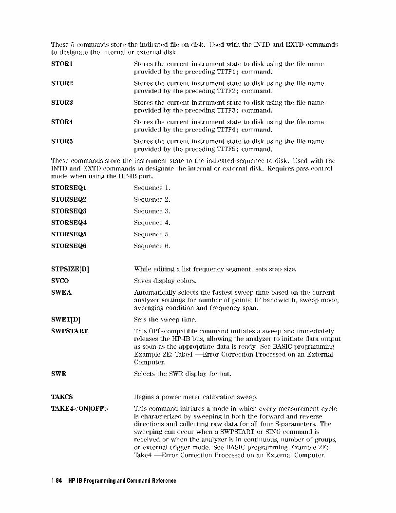
These 5 commands store the indicated �le on disk. Used with the INTD and EXTD commands
to designate the internal or external disk.
STOR1 Stores the current instrument state to disk using the �le name
provided by the preceding TITF1; command.
STOR2 Stores the current instrument state to disk using the �le name
provided by the preceding TITF2; command.
STOR3 Stores the current instrument state to disk using the �le name
provided by the preceding TITF3; command.
STOR4 Stores the current instrument state to disk using the �le name
provided by the preceding TITF4; command.
STOR5 Stores the current instrument state to disk using the �le name
provided by the preceding TITF5; command.
These commands store the instrument state to the indicated sequence to disk. Used with the
INTD and EXTD commands to designate the internal or external disk. Requires pass control
mode when using the HP-IB port.
STORSEQ1 Sequence 1.
STORSEQ2 Sequence 2.
STORSEQ3 Sequence 3.
STORSEQ4 Sequence 4.
STORSEQ5 Sequence 5.
STORSEQ6 Sequence 6.
STPSIZE[D] While editing a list frequency segment, sets step size.
SVCO Saves display colors.
SWEA Automatically selects the fastest sweep time based on the current
analyzer settings for number of points, IF bandwidth, sweep mode,
averaging condition and frequency span.
SWET[D] Sets the sweep time.
SWPSTART This OPC-compatible command initiates a sweep and immediately
releases the HP-IB bus, allowing the analyzer to initiate data output
as soon as the appropriate data is ready. See BASIC programming
Example 2E: Take4 | Error Correction Processed on an External
Computer.
SWR Selects the SWR display format.
TAKCS Begins a power meter calibration sweep.
TAKE4<ONjOFF> This command initiates a mode in which every measurement cycle
is characterized by sweeping in both the forward and reverse
directions and collecting raw data for all four S-parameters. The
sweeping can occur when a SWPSTART or SING command is
received or when the analyzer is in continuous, number of groups,
or external trigger mode. See BASIC programming Example 2E:
Take4 | Error Correction Processed on an External Computer.
1-94 HP-IB Programming and Command Reference
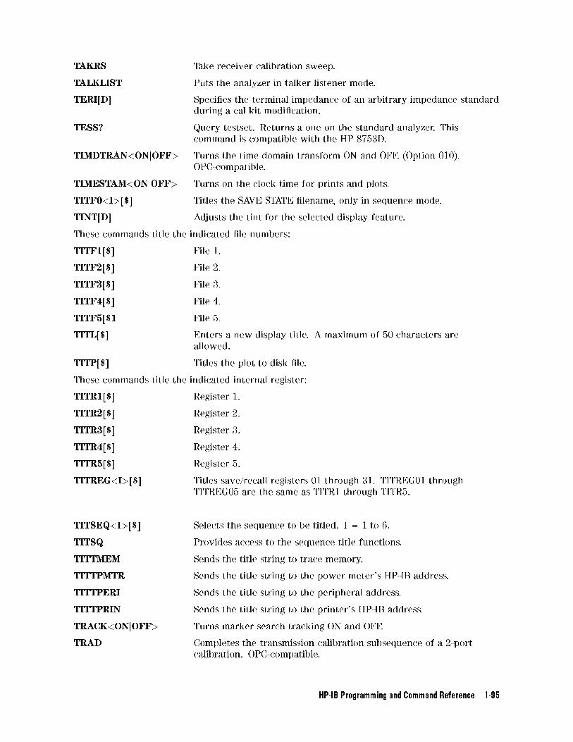
TAKRS Take receiver calibration sweep.
TALKLIST Puts the analyzer in talker listener mode.
TERI[D] Speci�es the terminal impedance of an arbitrary impedance standard
during a cal kit modi�cation.
TESS? Query testset. Returns a one on the standard analyzer. This
command is compatible with the HP 8753D.
TIMDTRAN<ONjOFF> Turns the time domain transform ON and OFF. (Option 010).
OPC-compatible.
TIMESTAM<ONjOFF> Turns on the clock time for prints and plots.
TITF0<I>[$] Titles the SAVE STATE �lename, only in sequence mode.
TINT[D] Adjusts the tint for the selected display feature.
These commands title the indicated �le numbers:
TITF1[$] File 1.
TITF2[$] File 2.
TITF3[$] File 3.
TITF4[$] File 4.
TITF5[$1 File 5.
TITL[$] Enters a new display title. A maximum of 50 characters are
allowed.
TITP[$] Titles the plot to disk �le.
These commands title the indicated internal register:
TITR1[$] Register 1.
TITR2[$] Register 2.
TITR3[$] Register 3.
TITR4[$] Register 4.
TITR5[$] Register 5.
TITREG<I>[$] Titles save/recall registers 01 through 31. TITREG01 through
TITREG05 are the same as TITR1 through TITR5.
TITSEQ<I>[$] Selects the sequence to be titled. I = 1 to 6.
TITSQ Provides access to the sequence title functions.
TITTMEM Sends the title string to trace memory.
TITTPMTR Sends the title string to the power meter's HP-IB address.
TITTPERI Sends the title string to the peripheral address.
TITTPRIN Sends the title string to the printer's HP-IB address.
TRACK<ONjOFF> Turns marker search tracking ON and OFF.
TRAD Completes the transmission calibration subsequence of a 2-port
calibration. OPC-compatible.
HP-IB Programming and Command Reference 1-95
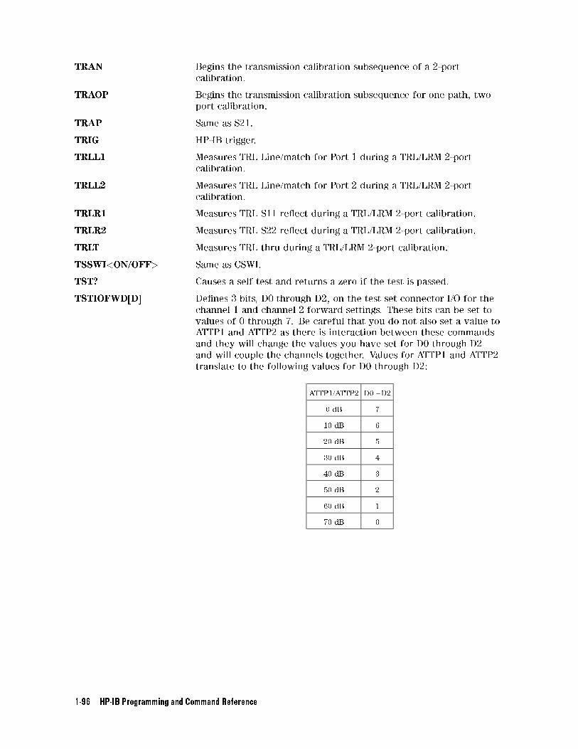
TRAN Begins the transmission calibration subsequence of a 2-port
calibration.
TRAOP Begins the transmission calibration subsequence for one path, two
port calibration.
TRAP Same as S21.
TRIG HP-IB trigger.
TRLL1 Measures TRL Line/match for Port 1 during a TRL/LRM 2-port
calibration.
TRLL2 Measures TRL Line/match for Port 2 during a TRL/LRM 2-port
calibration.
TRLR1 Measures TRL S11 re ect during a TRL/LRM 2-port calibration.
TRLR2 Measures TRL S22 re ect during a TRL/LRM 2-port calibration.
TRLT Measures TRL thru during a TRL/LRM 2-port calibration.
TSSWI<ON/OFF> Same as CSWI.
TST? Causes a self test and returns a zero if the test is passed.
TSTIOFWD[D] De�nes 3 bits, D0 through D2, on the test set connector I/O for the
channel 1 and channel 2 forward settings. These bits can be set to
values of 0 through 7. Be careful that you do not also set a value to
ATTP1 and ATTP2 as there is interaction between these commands
and they will change the values you have set for D0 through D2
and will couple the channels together. Values for ATTP1 and ATTP2
translate to the following values for D0 through D2:
ATTP1/ATTP2 D0 - D2
0 dB 7
10 dB 6
20 dB 5
30 dB 4
40 dB 3
50 dB 2
60 dB 1
70 dB 0
1-96 HP-IB Programming and Command Reference
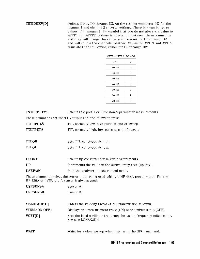
TSTIOREV[D] De�nes 3 bits, D0 through D2, on the test set connector I/O for the
channel 1 and channel 2 reverse settings. These bits can be set to
values of 0 through 7. Be careful that you do not also set a value to
ATTP1 and ATTP2 as there is interaction between these commands
and they will change the values you have set for D0 through D2
and will couple the channels together. Values for ATTP1 and ATTP2
translate to the following values for D0 through D2:
ATTP1/ATTP2 D0 - D2
0 dB 7
10 dB 6
20 dB 5
30 dB 4
40 dB 3
50 dB 2
60 dB 1
70 dB 0
TSTP<P1jP2> Selects test port 1 or 2 for non-S-parameter measurements.
These commands set the TTL output and end of sweep pulse:
TTLHPULS TTL normally low, high pulse at end of sweep.
TTLLPULS TTL normally high, low pulse at end of sweep.
TTLOH Sets TTL continuously high.
TTLOL Sets TTL continuously low.
UCONV Selects up converter for mixer measurements.
UP Increments the value in the active entry area (up key).
USEPASC Puts the analyzer in pass control mode.
These commands select the sensor input being used with the HP 438A power meter. For the
HP 436A or 437B, the A sensor is always used:
USESENSA Sensor A.
USESENSB Sensor B.
VELOFACT[D] Enters the velocity factor of the transmission medium.
VIEM<ONjOFF> Displays the measurement trace (ON) or the mixer setup (OFF).
VOFF[D] Sets the local oscillator frequency for use in frequency o�set mode.
See also LOFREQ[D].
WAIT Waits for a clean sweep when used with the OPC command.
HP-IB Programming and Command Reference 1-97
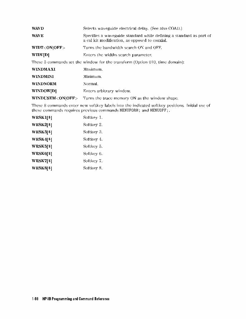
WAVD Selects waveguide electrical delay. (See also COAD.)
WAVE Speci�es a waveguide standard while de�ning a standard as part of
a cal kit modi�cation, as opposed to coaxial.
WIDT<ONjOFF> Turns the bandwidth search ON and OFF.
WIDV[D] Enters the widths search parameter.
These 5 commands set the window for the transform (Option 010, time domain):
WINDMAXI Maximum.
WINDMINI Minimum.
WINDNORM Normal.
WINDOW[D] Enters arbitrary window.
WINDUSEM<ONjOFF> Turns the trace memory ON as the window shape.
These 8 commands enter new softkey labels into the indicated softkey positions. Initial use of
these commands requires previous commands MENUFORM; and MENUOFF;.
WRSK1[$] Softkey 1.
WRSK2[$] Softkey 2.
WRSK3[$] Softkey 3.
WRSK4[$] Softkey 4.
WRSK5[$] Softkey 5.
WRSK6[$] Softkey 6.
WRSK7[$] Softkey 7.
WRSK8[$] Softkey 8.
1-98 HP-IB Programming and Command Reference
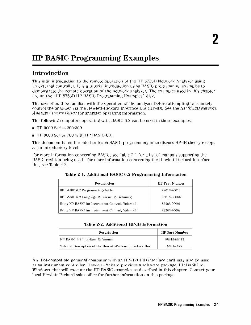
2
HP BASIC Programming Examples
Introduction
This is an introduction to the remote operation of the HP 8753D Network Analyzer using
an external controller. It is a tutorial introduction using BASIC programming examples to
demonstrate the remote operation of the network analyzer. The examples used in this chapter
are on the \HP 8753D HP BASIC Programming Examples" disk.
The user should be familiar with the operation of the analyzer before attempting to remotely
control the analyzer via the Hewlett-Packard Interface Bus (HP-IB). See the HP 8753D Network
Analyzer User's Guide for analyzer operating information.
The following computers operating with BASIC 6.2 can be used in these examples:
HP 9000 Series 200/300
HP 9000 Series 700 with HP BASIC-UX
This document is not intended to teach BASIC programming or to discuss HP-IB theory except
at an introductory level.
For more information concerning BASIC, see Table 2-1 for a list of manuals supporting the
BASIC revision being used. For more information concerning the Hewlett-Packard Interface
Bus, see Table 2-2.
Table 2-1. Additional BASIC 6.2 Programming Information
Description HP Part Number
HP BASIC 6.2 Programming Guide 98616-90010
HP BASIC 6.2 Language Reference (2 Volumes) 98616-90004
Using HP BASIC for Instrument Control, Volume I 82303-90001
Using HP BASIC for Instrument Control, Volume II 82303-90002
Table 2-2. Additional HP-IB Information
Description HP Part Number
HP BASIC 6.2 Interface Reference 98616-90013
Tutorial Description of the Hewlett-Packard Interface Bus 5021-1927
An IBM-compatible personal computer with an HP-IB/GPIB interface card may also be used
as an instrument controller. Hewlett-Packard provides a software package, HP BASIC for
Windows, that will execute the HP BASIC examples as described in this chapter. Contact your
local Hewlett-Packard sales o�ce for further information on this package.
HP BASIC Programming Examples 2-1
Required Equipment
Computer : : : : : : : : : : : : : : : : : : : : : : : : : : : : : : : : : : : : : : : : : : : : : : : : : : : : : : : : : : : : : : : : : : : : : : : : :HP 9000 Series
BASIC operating system: : : : : : : : : : : : : : : : : : : : : : : : : : : : : : : : : : : : : : : : : : : : : : : : : : : : : : : : : : : : : : : :BASIC 6.2
HP BASIC Programming Examples disk : : : : : : : : : : : : : : : : : : : : : : : : : : : : : : : : : : : : : : : : : : : : : 08753-10028
HP-IB interconnect cables : : : : : : : : : : : : : : : : : : : : : : : : : : : : : : : : : : : : : : : : : : : : : : : : : : : : :HP 10833A/B/C/D
Test device : : : : : : : : : : : : : : : : : : : : : : : : : : : : : : : : : : : : : : : : : : : : : : : : : : : : such as a 125 MHz bandpass �lter
Note The test device shipped with the instrument is a 10.24 GHz bandpass �lter. If
you wish to use this device, the frequency ranges of the example programs
must be modi�ed accordingly.
Note The computer must have enough memory to store:
BASIC 6.2 (4 MBytes of memory is required)
the required binaries
Upon receipt, make copies of the \Programming Examples" disks. Label them
\Programming Examples BACKUP". These disks will act as reserves in the
event of loss or damage to the original disks.
Optional Equipment
See the \Compatible Peripherals" chapter in the HP 8753D Network Analyzer User's Guide for
complete information on the following optional equipment:
Calibration kits
Test port return cables
Plotter
Printer
Disk drive
System Setup and HP-IB Veri�cation
This section describes how to:
Connect the test system.
Set the test system addresses.
Set the network analyzer's control mode.
Verify the operation of the system's interface bus (HP-IB).
2-2 HP BASIC Programming Examples
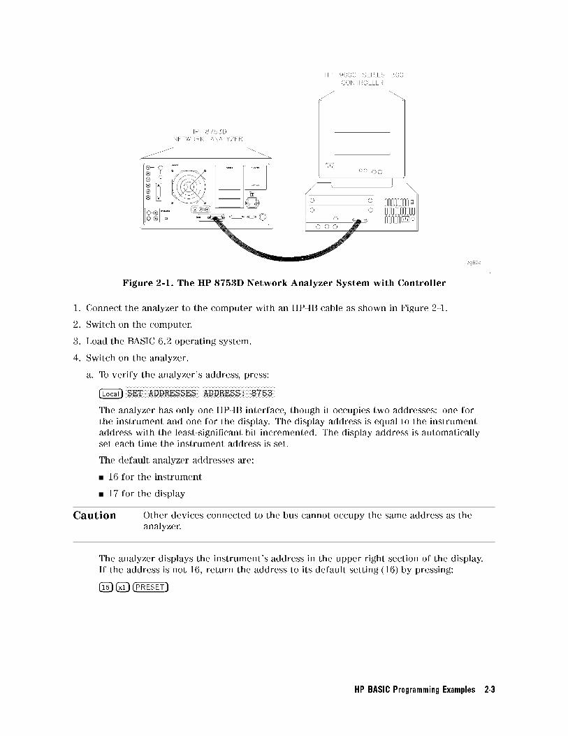
Figure 2-1. The HP 8753D Network Analyzer System with Controller
1. Connect the analyzer to the computer with an HP-IB cable as shown in Figure 2-1.
2. Switch on the computer.
3. Load the BASIC 6.2 operating system.
4. Switch on the analyzer.
a. To verify the analyzer's address, press:
�Local�NNNNNNNNNNNNNNNNNNNNNNNNNNNNNNNNNNNNNNNNNSET ADDRESSES
NNNNNNNNNNNNNNNNNNNNNNNNNNNNNNNNNNNNNNNNNADDRESS: 8753
The analyzer has only one HP-IB interface, though it occupies two addresses: one for
the instrument and one for the display. The display address is equal to the instrument
address with the least-signi�cant bit incremented. The display address is automatically
set each time the instrument address is set.
The default analyzer addresses are:
16 for the instrument
17 for the display
Caution Other devices connected to the bus cannot occupy the same address as the
analyzer.
The analyzer displays the instrument's address in the upper right section of the display.
If the address is not 16, return the address to its default setting (16) by pressing:
�16� �x1� �PRESET�
HP BASIC Programming Examples 2-3
b. Set the system control mode to either \pass-control" or \talker/listener" mode. These
are the only control modes in which the analyzer will accept commands over HP-IB. For
more information on control modes, see Chapter 1, \HP-IB Programming and Command
Reference." To set the system-control mode, press:
�Local�NNNNNNNNNNNNNNNNNNNNNNNNNNNNNNNNNNNNNNNNNNNNNNNTALKER/LISTENER
or
�Local�NNNNNNNNNNNNNNNNNNNNNNNNNNNNNNNNNNNNNNNNNNNNNNNNNNUSE PASS CONTROL
5. Check the interface bus by performing a simple command from the computer controller.
Type the following command on the controller:
OUTPUT 716;"PRES;" �EXECUTE� or �RETURN�
Note HP 9000 Series 300 computers use the �RETURN� key as both execute and enter.
Some other computers may have an �ENTER�, �EXECUTE�, or �EXEC� key that
performs the same function. For reasons of simplicity, the notation �RETURN� isused throughout this chapter.
This command should preset the analyzer. If an instrument preset does not occur, there is a
problem. Check all HP-IB addresses and connections. Most HP-IB problems are caused by an
incorrect address and faulty/loose HP-IB cables.
2-4 HP BASIC Programming Examples
HP 8753D Network Analyzer Instrument Control Using BASIC
A remote controller can manipulate the functions of the analyzer by sending commands to the
analyzer via the Hewlett-Packard Interface Bus (HP-IB). The commands used are speci�c to the
analyzer. Remote commands executed over the bus take precedence over manual commands
executed from the instrument's front panel. Remote commands are executed as soon as they
are received by the analyzer. A command only applies to the active channel (except in cases
where functions are coupled between channels). Most commands are equivalent to front-panel
hardkeys and softkeys.
Command Structure in BASIC
Consider the BASIC command for setting the analyzer's start frequency to 50 MHz:
OUTPUT 716;"STAR 50 MHZ;"
The command structure in BASIC has several di�erent elements:
the BASIC command statement OUTPUT - The BASIC data-output statement.
the appendage 716 - The data is directed to interface 7 (HP-IB), and
on to the device at address 16 (the analyzer). This
appendage is terminated with a semicolon. The next
appendage is STAR, the instrument mnemonic for
setting the analyzer's start frequency.
data 50 - a single operand used by the root mnemonic
STAR to set the value.
unit MHZ - the units that the operand is expressed in.
terminator ; - indicates the end of a command, enters the data,
and deactivates the active-entry area.
The "STAR 50 MHZ;" command performs the same function as pressing the following keys on
the analyzer's front panel:
�START� �50� �M/u�
STAR is the root mnemonic for the start key, 50 is the data, and MHZ are the units. Where
possible, the analyzer's root mnemonics are derived from the equivalent key label. Otherwise
they are derived from the common name for the function. Chapter 1, \HP-IB Programming and
Command Reference," lists all the root mnemonics and all the di�erent units accepted.
The semicolon (;) following MHZ terminates the command within the analyzer. It removes start
frequency from the active-entry area, and prepares the analyzer for the next command. If
there is a syntax error in a command, the analyzer will ignore the command and look for the
next terminator. When it �nds the next terminator, it starts processing incoming commands
normally. Characters between the syntax error and the next terminator are lost. A line feed
also acts as a terminator. The BASIC OUTPUT statement transmits a carriage return/line feed
following the data. This can be suppressed by putting a semicolon at the end of the statement.
The OUTPUT 716; statement will transmit all items listed (as long as they are separated by
commas or semicolons) including:
literal information enclosed in quotes,
numeric variables,
string variables,
and arrays.
A carriage return/line feed is transmitted after each item. Again, this can be suppressed by
terminating the commands with a semicolon. The analyzer automatically goes into remote
HP BASIC Programming Examples 2-5
mode when it receives an OUTPUT command from the controller. When this happens, the
front-panel remote (R) and listen (L) HP-IB status indicators illuminate. In remote mode, the
analyzer ignores any data that is input with the front-panel keys, with the exception of �Local�.Pressing �Local� returns the analyzer to manual operation, unless the universal HP-IB command
LOCAL LOCKOUT 7 has been issued. There are two ways to exit from a local lockout. Either
issue the LOCAL 7 command from the controller or cycle the line power on the analyzer.
Setting a parameter such as start frequency is just one form of command the analyzer will
accept. It will also accept simple commands that require no operand at all. For example,
execute:
OUTPUT 716;"AUTO;"
In response, the analyzer autoscales the active channel. Autoscale only applies to the active
channel, unlike start frequency, which applies to both channels as long as the channels are
stimulus-coupled.
The analyzer will also accept commands that switch various functions ON and OFF. For
example, to switch on dual-channel display, execute:
OUTPUT 716;"DUACON;"
DUACON is the analyzer root mnemonic for \dual-channel display on". This causes the analyzer
to display both channels. To go back to single-channel display mode, for example, switch o�
dual-channel display, execute:
OUTPUT 716;"DUACOFF;"
The construction of the command starts with the root mnemonic DUAC (dual-channel display,)
and ON or OFF is appended to the root to form the entire command.
The analyzer does not distinguish between upper- and lower-case letters. For example, execute:
OUTPUT 716;"auto;"
Note The analyzer also has a debug mode to aid in troubleshooting systems.
When the debug mode is ON, the analyzer scrolls incoming HP-IB commands
across the display. To manually activate the debug mode, press �Local�NNNNNNNNNNNNNNNNNNNNNNNNNNNNNNNNNNNNNNNNNHP-IB DIAG ON . To deactivate the debug mode from the controller, execute:
OUTPUT 716;"DEBUOFF;"
Command Query
Suppose the operator has changed the power level from the front panel. The computer can
�nd the new power level using the analyzer's command-query function. If a question mark is
appended to the root of a command, the analyzer will output the value of that function.
For instance, POWE 7 DB; sets the analyzer's output power to 7 dB, and POWE?; outputs the
current RF output power at the test port to the system controller. For example:
Type SCRATCH and press �RETURN� to clear old programs.
Type EDIT and press �RETURN� to access the edit mode.
2-6 HP BASIC Programming Examples
Then type in:
10 OUTPUT 716;"POWE?;"
20 ENTER 716;Reply
30 DISP Reply
40 END
Running the Program
The computer will display the preset source-power level in dBm. Change the power level by
pressing �Local� �Menu�NNNNNNNNNNNNNNNNNPOWER �XX� �x1�. Now run the program again.
When the analyzer receives POWE?, it prepares to transmit the current RF source-power level.
The BASIC statement ENTER 716 allows the analyzer to transmit information to the computer
by addressing the analyzer to talk. This illuminates the analyzer front-panel talk (T) light. The
computer places the data transmitted by the analyzer into the variables listed in the ENTER
statement. In this case, the analyzer transmits the output power, which gets placed in the
variable Reply.
The ENTER statement takes the stream of binary-data output from the analyzer and reformats
it back into numbers and ASCII strings. With the formatting set to its default state, the ENTER
statement will format the data into real variables, integers, or ASCII strings, depending on
the variable being �lled. The variable list must match the data the analyzer has to transmit.
If there are not enough variables, data is lost. If there are too many variables for the data
available, a BASIC error is generated.
The formatting done by the ENTER statement can be changed. For more information on data
formatting, see Chapter 1, \HP-IB Programming and Command Reference" under the section
titled \Array Data Formats." The formatting can be deactivated to allow binary transfers of
data. Also, the ENTER USING statement can be used to selectively control the formatting.
ON/OFF commands can be also be queried. The reply is a one (1) if the function is active, a
zero (0) if it is not active. Similarly, if a command controls a function that is underlined on the
analyzer softkey menu when active, querying that command yields a one (1) if the command is
underlined, a zero (0) if it is not. For example, press �Meas�. Though there are seven options on
the measurement menu, only one is underlined at a time. The underlined option will return a
one (1) when queried.
For instance, rewrite line 10 as:
10 OUTPUT 716;"DUAC?;"
Run the program once and note the result. Then press �Local� �DISPLAY�NNNNNNNNNNNNNNNNNNNNNNNNNNNNNDUAL CHAN to toggle the
display mode, and run the program again.
Another example is to rewrite line 10 as:
10 OUTPUT 716;"PHAS?;"
In this case, the program will display a one (1) if phase is currently being displayed. Since the
command only applies to the active channel, the response to the PHAS? inquiry depends on
which channel is active.
HP BASIC Programming Examples 2-7
Operation Complete
Occasionally, there is a need to query the analyzer as to when certain analyzer operations
have completed. For instance, a program should not have the operator connect the next
calibration standard while the analyzer is still measuring the current one. To provide such
information, the analyzer has an \operation complete" reporting mechanism, or OPC command,
that will indicate when certain key commands have completed operation. The mechanism is
activated by sending either OPC or OPC? immediately before an OPC-compatible command.
When the command completes execution, bit 0 of the event-status register will be set. If OPC
was queried with OPC?, the analyzer will also output a one (1) when the command completes
execution.
As an example, type SCRATCH and press �RETURN�.
Type EDIT and press �RETURN�.
Type in the following program:
10 OUTPUT 716;"SWET 3 S;OPC?;SING;" Set the sweep time to 3 seconds, and OPC a
single sweep.
20 DISP "SWEEPING"
30 ENTER 716;Reply The program will halt at this point until the
analyzer completes the sweep and issues a
one (1).
40 DISP "DONE"
50 END
Running the Program
Running this program causes the computer to display the sweeping message as the instrument
executes the sweep. The computer will display DONE just as the instrument goes into hold.
When DONE appears, the program could then continue on, being assured that there is a valid
data trace in the instrument.
Preparing for Remote (HP-IB) Control
At the beginning of a program, the analyzer is taken from an unknown state and brought under
remote control. This is done with an abort/clear sequence. ABORT 7 is used to halt bus activity
and return control to the computer. CLEAR 716 will then prepare the analyzer to receive
commands by:
clearing syntax errors
clearing the input-command bu�er
clearing any messages waiting to be output
The abort/clear sequence readies the analyzer to receive HP-IB commands. The next step
involves programming a known state into the analyzer. The most convenient way to do this is
to preset the analyzer by sending the PRES (preset) command. If preset cannot be used, the
status-reporting mechanism may be employed. When using the status-reporting register, CLES
(Clear Status) can be transmitted to the analyzer to clear all of the status-reporting registers
and their enables.
Type SCRATCH and press �RETURN�.
2-8 HP BASIC Programming Examples
Type EDIT and press �RETURN�. Type in the following program:
10 ABORT 7 This halts all bus action and gives active control to the computer.
20 CLEAR 716 This clears all HP-IB errors, resets the HP-IB interface, and
clears the syntax errors. It does not a�ect the status-reporting
system.
30 OUTPUT 716;"PRES;" Presets the instrument. This clears the status-reporting system,
as well as resets all of the front-panel settings, except for the HP-
IB mode and the HP-IB addresses.
40 END Running this program brings the analyzer to a known state,
ready to respond to HP-IB control.
The analyzer will not respond to HP-IB commands unless the remote line is asserted. When the
remote line is asserted, the analyzer is addressed to listen for commands from the controller.
In remote mode, all the front-panel keys are disabled (with the exception of �Local� and the
line-power switch). ABORT 7 asserts the remote line, which remains asserted until a LOCAL 7
statement is executed. Another way to assert the remote line is to execute:
REMOTE 716
This statement asserts the analyzer's remote-operation mode and addresses the analyzer to
listen for commands from the controller. Press any front-panel key except �Local�. Note thatnone of the front-panel keys will respond until �Local� has been pressed.
�Local� can also be disabled with the sequence:
REMOTE 716
LOCAL LOCKOUT 7
After executing the code above, none of front-panel keys will respond. The analyzer can be
returned to local mode temporarily with:
LOCAL 716
As soon as the analyzer is addressed to listen, it goes back into local-lockout mode. The only
way to clear the local- lockout mode, aside from cycling line power, is to execute:
LOCAL 7
This command un-asserts the remote line on the interface. This puts the instrument into
local mode and clears the local-lockout command. Return the instrument to remote mode by
pressing:
�Local�NNNNNNNNNNNNNNNNNNNNNNNNNNNNNNNNNNNNNNNNNNNNNNNTALKER/LISTENER
or
�Local�NNNNNNNNNNNNNNNNNNNNNNNNNNNNNNNNNNNNNNNNNNNNNNNNNNUSE PASS CONTROL
HP BASIC Programming Examples 2-9
I/O Paths
One of the features of HP BASIC is the use of input/output paths. The instrument may be
addressed directly by the instrument's device number as shown in the previous examples.
However, a more sophisticated approach is to declare I/O paths such as: ASSIGN @Nwa TO
716. Assigning an I/O path builds a look-up table in the computer's memory that contains the
device-address codes and several other parameters. It is easy to quickly change addresses
throughout the entire program at one location. I/O operation is more e�cient because it uses
a table, in place of calculating or searching for values related to I/O. In the more elaborate
examples where �le I/O is discussed, the look-up table contains all the information about the
�le. Execution time is decreased, because the computer no longer has to calculate a device's
address each time that device is addressed.
For example:
Type SCRATCH and press �RETURN�.
Type EDIT and press �RETURN�.
Type in the following program:
10 ASSIGN @Nwa TO 716 Assigns the analyzer to ADDRESS 716.
20 OUTPUT @Nwa;"STAR 50 MHZ;" Sets the analyzer's start frequency to 50 MHz.
Note The use of I/O paths in binary-format transfers allows the user to quickly
distinguish the type of transfer taking place. I/O paths are used throughout the
examples and are highly recommended for use in device input/output.
2-10 HP BASIC Programming Examples
Measurement Process
This section explains how to organize instrument commands into a measurement sequence. A
typical measurement sequence consists of the following steps:
1. setting up the instrument
2. calibrating the test setup
3. connecting the device under test
4. taking the measurement data
5. post-processing the measurement data
6. transferring the measurement data
Step 1. Setting Up the Instrument
De�ne the measurement by setting all of the basic measurement parameters. These include:
the sweep type
the frequency span
the sweep time
the number of points (in the data trace)
the RF power level
the type of measurement
the IF averaging
the IF bandwidth
You can quickly set up an entire instrument state, using the save/recall registers and the learn
string. The learn string is a summary of the instrument state compacted into a string that the
computer reads and retransmits to the analyzer. See \Example 5A: Using the Learn String."
Step 2. Calibrating the Test Setup
After you have de�ned an instrument state, you should perform a measurement calibration.
Although it is not required, a measurement calibration improves the accuracy of your
measurement data.
The following list describes several methods to calibrate the analyzer:
Stop the program and perform a calibration from the analyzer's front panel.
Use the computer to guide you through the calibration, as discussed in:
\Example 2A: S11 1-Port Measurement Calibration."
\Example 2B: Full 2-Port Measurement Calibration."
\Example 2C: Adapter Removal Calibration."
\Example 2D: Using Raw Data to Create a Calibration (Simmcal)."
\Example 2E: Take4 | Error Correction Processed on an External PC."
Transfer the calibration data from a previous calibration back into the analyzer, as discussed
in \Example 5C: Saving and Restoring the Analyzer Instrument State."
HP BASIC Programming Examples 2-11
Step 3. Connecting the Device under Test
After you connect your test device, you can use the computer to speed up any necessary
device adjustments such as limit testing, bandwidth searches, and trace statistics.
Step 4. Taking the Measurement Data
Measure the device response and set the analyzer to hold the data. This captures the data on
the analyzer display.
By using the single-sweep command (SING), you can insure a valid sweep. When you use this
command, the analyzer completes all stimulus changes before starting the sweep, and does not
release the HP-IB hold state until it has displayed the formatted trace. Then when the analyzer
completes the sweep, the instrument is put into hold mode, freezing the data. Because single
sweep is OPC-compatible, it is easy to determine when the sweep has been completed.
The number-of-groups command (NUMGn) triggers multiple sweeps. It is designed to work the
same as single-sweep command. NUMGn is useful for making a measurement with an averaging
factor n (n can be 1 to 999). Both the single-sweep and number-of-groups commands restart
averaging.
Step 5. Post-Processing the Measurement Data
Figure 1-4 shows the process functions used to a�ect the data after you have made an
error-corrected measurement. These process functions have parameters that can be adjusted
to manipulate the error-corrected data prior to formatting. They do not a�ect the analyzer's
data gathering. The most useful functions are trace statistics, marker searches, electrical-delay
o�set, time domain, and gating.
After Performing and activating a full 2-port measurement calibration, any of the four
S-parameters may be viewed without taking a new sweep.
Step 6. Transferring the Measurement Data
Read your measurement results. All the data-output commands are designed to insure that the
data transmitted re ects the current state of the instrument.
2-12 HP BASIC Programming Examples
BASIC Programming Examples
The following sample programs provide the user with factory-tested solutions for several
remotely-controlled analyzer processes. The programs can be used in their present state or
modi�ed to suit speci�c needs. The programs discussed in this section can be found on the
\HP 8753D HP BASIC Programming Examples" disk received with the analyzer.
Example 1: Measurement Setup
Example 1A: Setting Parameters
Example 1B: Verifying Parameters
Example 2: Measurement Calibration
Example 2A: S11 1-Port Measurement Calibration
Example 2B: Full 2-Port Measurement Calibration
Example 2C: Adapter Removal Calibration
Example 2D: Using Raw Data to Create a Calibration (Simmcal)
Example 2E: Take4 | Error Correction Processed on an External PC
Example 3: Measurement Data Transfer
Example 3A: Data Transfer Using Markers
Example 3B: Data Transfer Using FORM 4 (ASCII Transfer)
Example 3C: Data Transfer Using Floating-Point Numbers
Example 3D: Data Transfer Using Frequency�Array Information
Example 3E: Data Transfer Using FORM 1 (Internal Binary Format)
Example 4: Measurement Process Synchronization
Example 4A: Using the Error Queue
Example 4B: Generating Interrupts
Example 4C: Power Meter Calibration
Example 5: Network Analyzer System Setups
Example 5A: Using the Learn String
Example 5B: Reading Calibration Data
Example 5C: Saving and Restoring the Analyzer Instrument State
Example 6: Limit-Line Testing
Example 6A: Setting Up a List-Frequency Sweep
Example 6B: Selecting a Single Segment from a Table of Segments
Example 6C: Setting Up Limit Lines
Example 6D: Performing PASS/FAIL Tests While Tuning
Example 7: Report Generation
Example 7A1: Operation Using Talker/Listener Mode
Example 7A2: Controlling Peripherals Using Pass-Control Mode
Example 7A3: Printing with the Serial Port
HP BASIC Programming Examples 2-13
Example 7B: Plotting to a File and Transferring the File Data to a Plotter
Utilizing PC-Graphics Applications Using the Plot File
Example 7C: Reading ASCII Disk Files to the Instrument Controller's Disk File
Example 8: Mixer Measurements
Example 8A: Comparison of Two Mixers | Group Delay, Amplitude or Phase
Program Information
The following information is provided for every example program included on the
\Programming Examples" disk:
A program description
An outline of the program's processing sequence
A step-by-step instrument-command-level tutorial explanation of the program including:
The command mnemonic and command name for the HP-IB instrument command used in
the program.
An explanation of the operations and a�ects of the HP-IB instrument commands used in
the program.
Note The HP BASIC programming code for each of these examples is contained in
\HP BASIC Programming Examples."
Analyzer Features Helpful in Developing Programming Routines
Analyzer-Debug Mode
The analyzer-debug mode aids you in developing programming routines. The analyzer displays
the commands being received. If a syntax error occurs, the analyzer displays the last bu�er
and points to the �rst character in the command line that it could not understand.
You can enable this mode from the front panel by pressing �Local�NNNNNNNNNNNNNNNNNNNNNNNNNNNNNNNNNNNNNNNNNHP-IB DIAG ON . The debug
mode remains activated until you preset the analyzer or deactivate the mode. You can also
enable this mode over the HP-IB using the DEBUON; command and disable the debug mode
using the DEBUOFF; command.
User-Controllable Sweep
There are three important advantages to using the single-sweep mode:
1. The user can initiate the sweep.
2. The user can determine when the sweep has completed.
3. The user can be con�dent that the trace data has be derived from a valid sweep.
Execute the command string OPC?;SING; to place the analyzer in single-sweep mode and
trigger a sweep. Once the sweep is complete, the analyzer returns an ASCII character one (1) to
indicate the completion of the sweep.
Note The measurement cycle and the data acquisition cycle must always be
synchronized. The analyzer must complete a measurement sweep for the data
to be valid.
2-14 HP BASIC Programming Examples
Example 1: Measurement Setup
The programs included in Example 1 provide the user the option to perform instrument-setup
functions for the analyzer from a remote controller. Example 1A is a program designed to
setup the analyzer's measurement parameters. Example 1B is a program designed to verify the
measurement parameters.
Example 1A: Setting Parameters
Note This program is stored as EXAMP1A on the \Programming Examples" disk
received with the network analyzer.
In general, the procedure for setting up measurements on the network analyzer via HP-IB
follows the same sequence as if the setup was performed manually. There is no required order,
as long as the desired frequency range, number of points, and power level are set prior to
performing the calibration �rst, and the measurement second.
This example sets the following parameters:
re ection log magnitude on channel 1
re ection phase on channel 2
dual channel display mode
frequency range from 100 MHz to 500 MHz
The following is an outline of the program's processing sequence:
An I/O path is assigned for the analyzer.
The system is initialized.
The analyzer is adjusted to measure return loss (S11) on channel 1 and display it in log
magnitude.
The analyzer is adjusted to measure return loss (S11) on channel 2 and display the phase.
The dual-channel display mode is activated.
The system operator is prompted to enter the frequency range of the measurement.
The displays are autoscaled.
The analyzer is released from remote control and the program ends.
HP BASIC Programming Examples 2-15
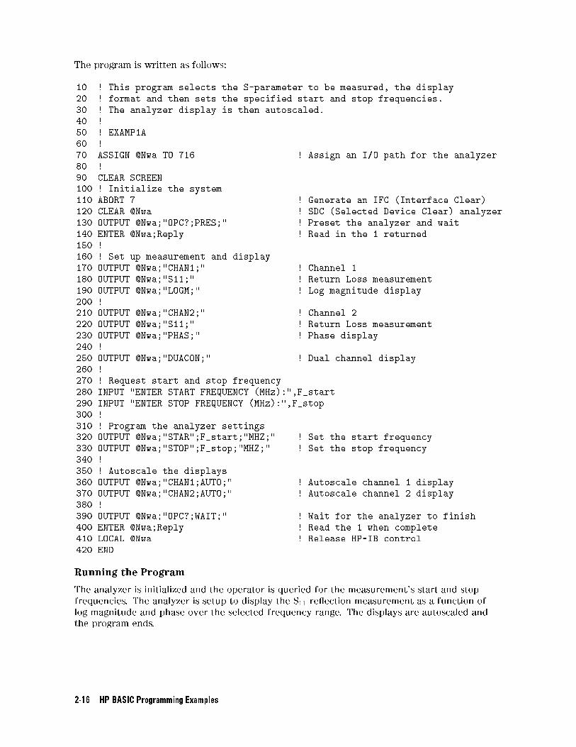
The program is written as follows:
10 ! This program selects the S-parameter to be measured, the display
20 ! format and then sets the specified start and stop frequencies.
30 ! The analyzer display is then autoscaled.
40 !
50 ! EXAMP1A
60 !
70 ASSIGN @Nwa TO 716 ! Assign an I/O path for the analyzer
80 !
90 CLEAR SCREEN
100 ! Initialize the system
110 ABORT 7 ! Generate an IFC (Interface Clear)
120 CLEAR @Nwa ! SDC (Selected Device Clear) analyzer
130 OUTPUT @Nwa;"OPC?;PRES;" ! Preset the analyzer and wait
140 ENTER @Nwa;Reply ! Read in the 1 returned
150 !
160 ! Set up measurement and display
170 OUTPUT @Nwa;"CHAN1;" ! Channel 1
180 OUTPUT @Nwa;"S11;" ! Return Loss measurement
190 OUTPUT @Nwa;"LOGM;" ! Log magnitude display
200 !
210 OUTPUT @Nwa;"CHAN2;" ! Channel 2
220 OUTPUT @Nwa;"S11;" ! Return Loss measurement
230 OUTPUT @Nwa;"PHAS;" ! Phase display
240 !
250 OUTPUT @Nwa;"DUACON;" ! Dual channel display
260 !
270 ! Request start and stop frequency
280 INPUT "ENTER START FREQUENCY (MHz):",F_start
290 INPUT "ENTER STOP FREQUENCY (MHz):",F_stop
300 !
310 ! Program the analyzer settings
320 OUTPUT @Nwa;"STAR";F_start;"MHZ;" ! Set the start frequency
330 OUTPUT @Nwa;"STOP";F_stop;"MHZ;" ! Set the stop frequency
340 !
350 ! Autoscale the displays
360 OUTPUT @Nwa;"CHAN1;AUTO;" ! Autoscale channel 1 display
370 OUTPUT @Nwa;"CHAN2;AUTO;" ! Autoscale channel 2 display
380 !
390 OUTPUT @Nwa;"OPC?;WAIT;" ! Wait for the analyzer to finish
400 ENTER @Nwa;Reply ! Read the 1 when complete
410 LOCAL @Nwa ! Release HP-IB control
420 END
Running the Program
The analyzer is initialized and the operator is queried for the measurement's start and stop
frequencies. The analyzer is setup to display the S11 re ection measurement as a function of
log magnitude and phase over the selected frequency range. The displays are autoscaled and
the program ends.
2-16 HP BASIC Programming Examples
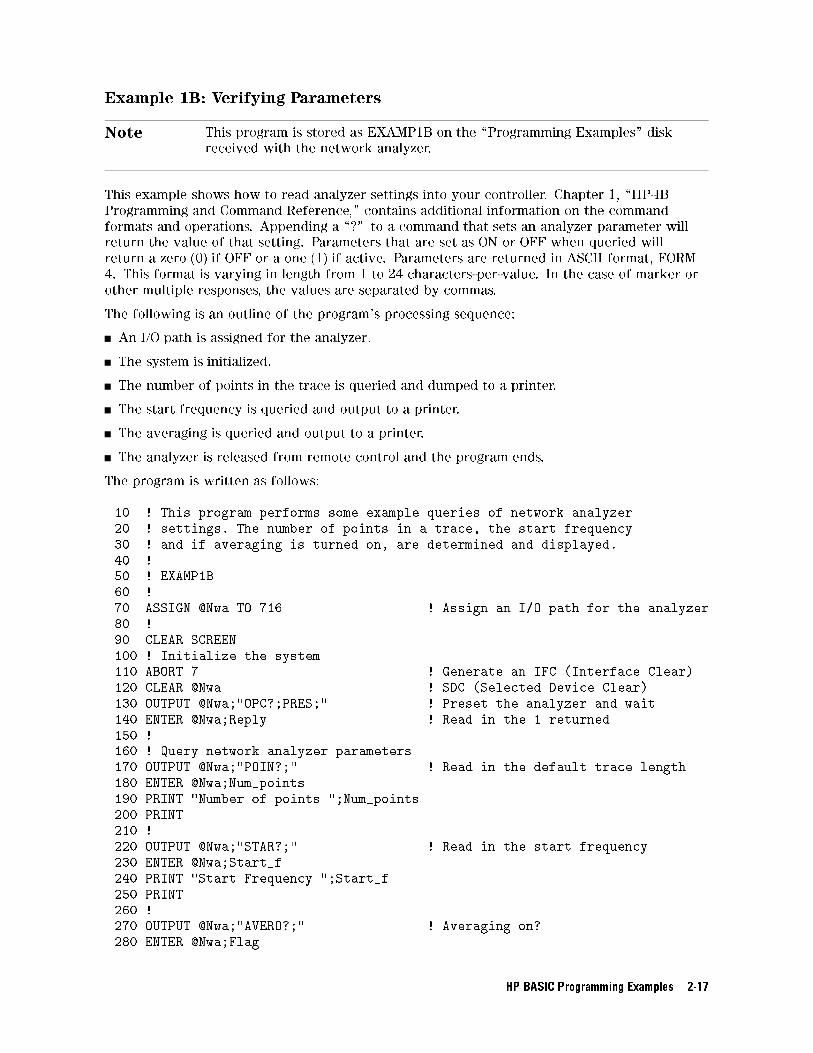
Example 1B: Verifying Parameters
Note This program is stored as EXAMP1B on the \Programming Examples" disk
received with the network analyzer.
This example shows how to read analyzer settings into your controller. Chapter 1, \HP-IB
Programming and Command Reference," contains additional information on the command
formats and operations. Appending a \?" to a command that sets an analyzer parameter will
return the value of that setting. Parameters that are set as ON or OFF when queried will
return a zero (0) if OFF or a one (1) if active. Parameters are returned in ASCII format, FORM
4. This format is varying in length from 1 to 24 characters-per-value. In the case of marker or
other multiple responses, the values are separated by commas.
The following is an outline of the program's processing sequence:
An I/O path is assigned for the analyzer.
The system is initialized.
The number of points in the trace is queried and dumped to a printer.
The start frequency is queried and output to a printer.
The averaging is queried and output to a printer.
The analyzer is released from remote control and the program ends.
The program is written as follows:
10 ! This program performs some example queries of network analyzer
20 ! settings. The number of points in a trace, the start frequency
30 ! and if averaging is turned on, are determined and displayed.
40 !
50 ! EXAMP1B
60 !
70 ASSIGN @Nwa TO 716 ! Assign an I/O path for the analyzer
80 !
90 CLEAR SCREEN
100 ! Initialize the system
110 ABORT 7 ! Generate an IFC (Interface Clear)
120 CLEAR @Nwa ! SDC (Selected Device Clear)
130 OUTPUT @Nwa;"OPC?;PRES;" ! Preset the analyzer and wait
140 ENTER @Nwa;Reply ! Read in the 1 returned
150 !
160 ! Query network analyzer parameters
170 OUTPUT @Nwa;"POIN?;" ! Read in the default trace length
180 ENTER @Nwa;Num_points
190 PRINT "Number of points ";Num_points
200 PRINT
210 !
220 OUTPUT @Nwa;"STAR?;" ! Read in the start frequency
230 ENTER @Nwa;Start_f
240 PRINT "Start Frequency ";Start_f
250 PRINT
260 !
270 OUTPUT @Nwa;"AVERO?;" ! Averaging on?
280 ENTER @Nwa;Flag
HP BASIC Programming Examples 2-17
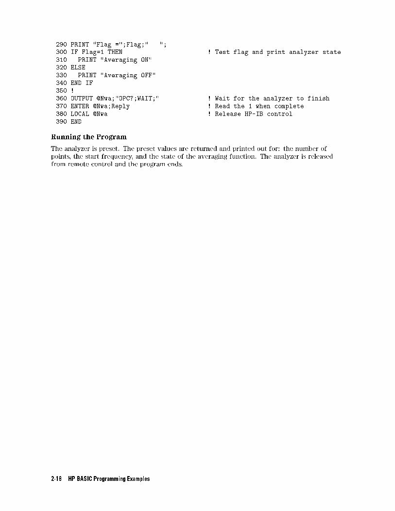
290 PRINT "Flag =";Flag;" ";
300 IF Flag=1 THEN ! Test flag and print analyzer state
310 PRINT "Averaging ON"
320 ELSE
330 PRINT "Averaging OFF"
340 END IF
350 !
360 OUTPUT @Nwa;"OPC?;WAIT;" ! Wait for the analyzer to finish
370 ENTER @Nwa;Reply ! Read the 1 when complete
380 LOCAL @Nwa ! Release HP-IB control
390 END
Running the Program
The analyzer is preset. The preset values are returned and printed out for: the number of
points, the start frequency, and the state of the averaging function. The analyzer is released
from remote control and the program ends.
2-18 HP BASIC Programming Examples
Example 2: Measurement Calibration
This section shows you how to coordinate a measurement calibration over HP-IB. You can use
the following sequence for performing either a manual measurement calibration, or a remote
measurement calibration via HP-IB:
1. Select the calibration type.
2. Measure the calibration standards.
3. Declare the calibration done.
The actual sequence depends on the calibration kit and changes slightly for 2-port calibrations,
which are divided into three calibration sub-sequences. The following examples are included:
Example 2A is a program designed to perform an S11 1-port measurement calibration.
Example 2B is a program designed to perform a full 2-port measurement calibration.
Example 2C is a program designed to accurately measure a \non-insertable" 2-port device,
using adapter removal.
Example 2D is a program designed to use raw data to create a calibration, sometimes called
Simmcal.
Example 2E is a program designed to o�oad the calculation of the 2-port error corrected
data to an external computer.
Calibration Kits
The calibration kit tells the analyzer what standards to expect at each step of the calibration.
The set of standards associated with a given calibration is termed a \class." For example,
measuring the short during an S11 1-port measurement calibration is one calibration step. All
of the shorts that can be used for this calibration step make up the class, which is called class
S11B. For the 7-mm and the 3.5-mm cal kits, class S11B uses only one standard. For type-N cal
kits, class S11B contains two standards: male and female shorts.
When doing an S11 1-port measurement calibration using a 7- or 3.5-mm calibration kit,
selectingNNNNNNNNNNNNNNNNNSHORT automatically measures the short because the class contains only one
standard. When doing the same calibration in type-N, selectingNNNNNNNNNNNNNNNNNSHORT brings up a second
menu, allowing the operator to select which standard in the class is to be measured. The sex
listed refers to the test port: if the test port is female, then the operator selects the female
short option. Once the standard has been selected and measured, theNNNNNNNNNNNNNNDONE key must be
pressed to exit the class.
Doing an S11 1-port measurement calibration over HP-IB is very similar. When using a 7- or
3.5-mm calibration kit, sending CLASS11B will automatically measure the short. In type-N,
sending CLASS11B brings up the menu with the male and female short options. To select a
standard, use STANA or STANB. The STAN command is appended with the letters A through G,
corresponding to the standards listed under softkeys 1 through 7, softkey 1 being the topmost
softkey.
The STAN command is OPC-compatible. A command that calls a class is only OPC-compatible
if that class has only one standard in it. If there is more than one standard in a class, the
command that calls the class brings up another menu, and there is no need to query it. DONE;
must be sent to exit the class.
HP BASIC Programming Examples 2-19
Example 2A: S11 1-Port Calibration
Note This program is stored as EXAMP2A on the \Programming Examples" disk
received with the network analyzer.
The following program performs an S11 1-port calibration, using either the HP 85031B
7-mm calibration kit or the HP 85033D 3.5-mm calibration kit. If you wish to use a di�erent
calibration kit, modify the example program accordingly. This program simpli�es the
calibration by providing explicit directions on the analyzer display while allowing the
user to run the program from the controller keyboard. More information on selecting
calibration standards can be found in the Optimizing Measurement Results chapter of the
HP 8753D/Option 011 Network Analyzer User's Guide.
The following is an outline of the program's processing sequence:
An I/O path is assigned for the analyzer.
The system is initialized.
The appropriate calibration kit is selected.
The softkey menu is deactivated.
The S11-calibration sequence is run.
The S11-calibration data is saved.
The softkey menu is activated.
The analyzer is released from remote control and the program ends.
2-20 HP BASIC Programming Examples
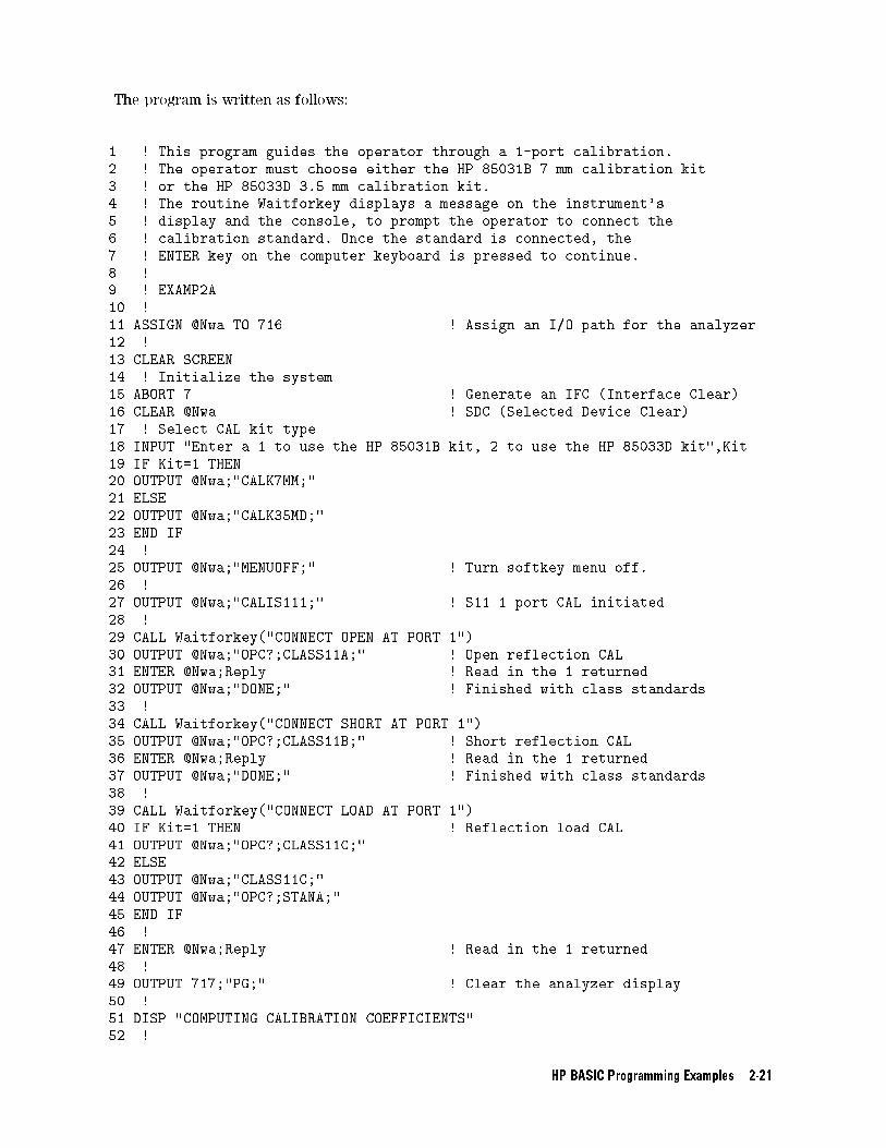
The program is written as follows:
1 ! This program guides the operator through a 1-port calibration.
2 ! The operator must choose either the HP 85031B 7 mm calibration kit
3 ! or the HP 85033D 3.5 mm calibration kit.
4 ! The routine Waitforkey displays a message on the instrument's
5 ! display and the console, to prompt the operator to connect the
6 ! calibration standard. Once the standard is connected, the
7 ! ENTER key on the computer keyboard is pressed to continue.
8 !
9 ! EXAMP2A
10 !
11 ASSIGN @Nwa TO 716 ! Assign an I/O path for the analyzer
12 !
13 CLEAR SCREEN
14 ! Initialize the system
15 ABORT 7 ! Generate an IFC (Interface Clear)
16 CLEAR @Nwa ! SDC (Selected Device Clear)
17 ! Select CAL kit type
18 INPUT "Enter a 1 to use the HP 85031B kit, 2 to use the HP 85033D kit",Kit
19 IF Kit=1 THEN
20 OUTPUT @Nwa;"CALK7MM;"
21 ELSE
22 OUTPUT @Nwa;"CALK35MD;"
23 END IF
24 !
25 OUTPUT @Nwa;"MENUOFF;" ! Turn softkey menu off.
26 !
27 OUTPUT @Nwa;"CALIS111;" ! S11 1 port CAL initiated
28 !
29 CALL Waitforkey("CONNECT OPEN AT PORT 1")
30 OUTPUT @Nwa;"OPC?;CLASS11A;" ! Open reflection CAL
31 ENTER @Nwa;Reply ! Read in the 1 returned
32 OUTPUT @Nwa;"DONE;" ! Finished with class standards
33 !
34 CALL Waitforkey("CONNECT SHORT AT PORT 1")
35 OUTPUT @Nwa;"OPC?;CLASS11B;" ! Short reflection CAL
36 ENTER @Nwa;Reply ! Read in the 1 returned
37 OUTPUT @Nwa;"DONE;" ! Finished with class standards
38 !
39 CALL Waitforkey("CONNECT LOAD AT PORT 1")
40 IF Kit=1 THEN ! Reflection load CAL
41 OUTPUT @Nwa;"OPC?;CLASS11C;"
42 ELSE
43 OUTPUT @Nwa;"CLASS11C;"
44 OUTPUT @Nwa;"OPC?;STANA;"
45 END IF
46 !
47 ENTER @Nwa;Reply ! Read in the 1 returned
48 !
49 OUTPUT 717;"PG;" ! Clear the analyzer display
50 !
51 DISP "COMPUTING CALIBRATION COEFFICIENTS"
52 !
HP BASIC Programming Examples 2-21
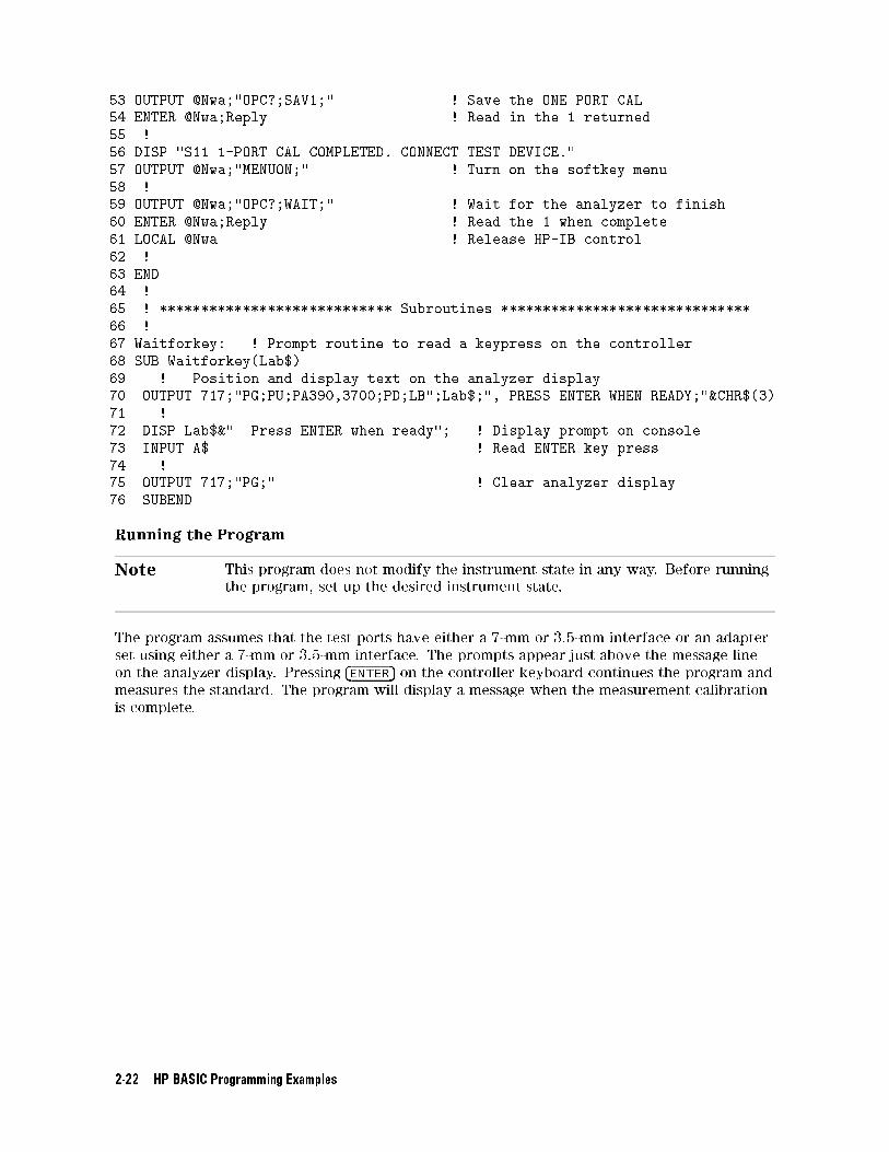
53 OUTPUT @Nwa;"OPC?;SAV1;" ! Save the ONE PORT CAL
54 ENTER @Nwa;Reply ! Read in the 1 returned
55 !
56 DISP "S11 1-PORT CAL COMPLETED. CONNECT TEST DEVICE."
57 OUTPUT @Nwa;"MENUON;" ! Turn on the softkey menu
58 !
59 OUTPUT @Nwa;"OPC?;WAIT;" ! Wait for the analyzer to finish
60 ENTER @Nwa;Reply ! Read the 1 when complete
61 LOCAL @Nwa ! Release HP-IB control
62 !
63 END
64 !
65 ! **************************** Subroutines ******************************
66 !
67 Waitforkey: ! Prompt routine to read a keypress on the controller
68 SUB Waitforkey(Lab$)
69 ! Position and display text on the analyzer display
70 OUTPUT 717;"PG;PU;PA390,3700;PD;LB";Lab$;", PRESS ENTER WHEN READY;"&CHR$(3)
71 !
72 DISP Lab$&" Press ENTER when ready"; ! Display prompt on console
73 INPUT A$ ! Read ENTER key press
74 !
75 OUTPUT 717;"PG;" ! Clear analyzer display
76 SUBEND
Running the Program
Note This program does not modify the instrument state in any way. Before running
the program, set up the desired instrument state.
The program assumes that the test ports have either a 7-mm or 3.5-mm interface or an adapter
set using either a 7-mm or 3.5-mm interface. The prompts appear just above the message line
on the analyzer display. Pressing �ENTER� on the controller keyboard continues the program and
measures the standard. The program will display a message when the measurement calibration
is complete.
2-22 HP BASIC Programming Examples
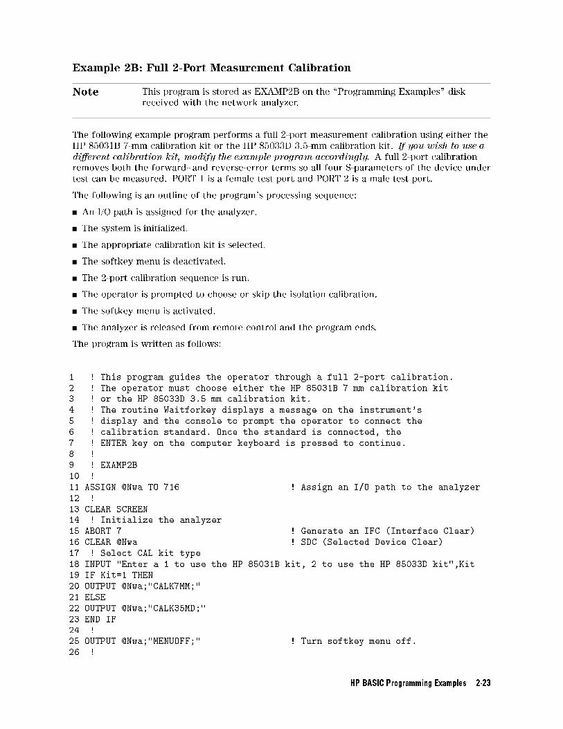
Example 2B: Full 2-Port Measurement Calibration
Note This program is stored as EXAMP2B on the \Programming Examples" disk
received with the network analyzer.
The following example program performs a full 2-port measurement calibration using either the
HP 85031B 7-mm calibration kit or the HP 85033D 3.5-mm calibration kit. If you wish to use a
di�erent calibration kit, modify the example program accordingly. A full 2-port calibration
removes both the forward- and reverse-error terms so all four S-parameters of the device under
test can be measured. PORT 1 is a female test port and PORT 2 is a male test port.
The following is an outline of the program's processing sequence:
An I/O path is assigned for the analyzer.
The system is initialized.
The appropriate calibration kit is selected.
The softkey menu is deactivated.
The 2-port calibration sequence is run.
The operator is prompted to choose or skip the isolation calibration.
The softkey menu is activated.
The analyzer is released from remote control and the program ends.
The program is written as follows:
1 ! This program guides the operator through a full 2-port calibration.
2 ! The operator must choose either the HP 85031B 7 mm calibration kit
3 ! or the HP 85033D 3.5 mm calibration kit.
4 ! The routine Waitforkey displays a message on the instrument's
5 ! display and the console to prompt the operator to connect the
6 ! calibration standard. Once the standard is connected, the
7 ! ENTER key on the computer keyboard is pressed to continue.
8 !
9 ! EXAMP2B
10 !
11 ASSIGN @Nwa TO 716 ! Assign an I/O path to the analyzer
12 !
13 CLEAR SCREEN
14 ! Initialize the analyzer
15 ABORT 7 ! Generate an IFC (Interface Clear)
16 CLEAR @Nwa ! SDC (Selected Device Clear)
17 ! Select CAL kit type
18 INPUT "Enter a 1 to use the HP 85031B kit, 2 to use the HP 85033D kit",Kit
19 IF Kit=1 THEN
20 OUTPUT @Nwa;"CALK7MM;"
21 ELSE
22 OUTPUT @Nwa;"CALK35MD;"
23 END IF
24 !
25 OUTPUT @Nwa;"MENUOFF;" ! Turn softkey menu off.
26 !
HP BASIC Programming Examples 2-23
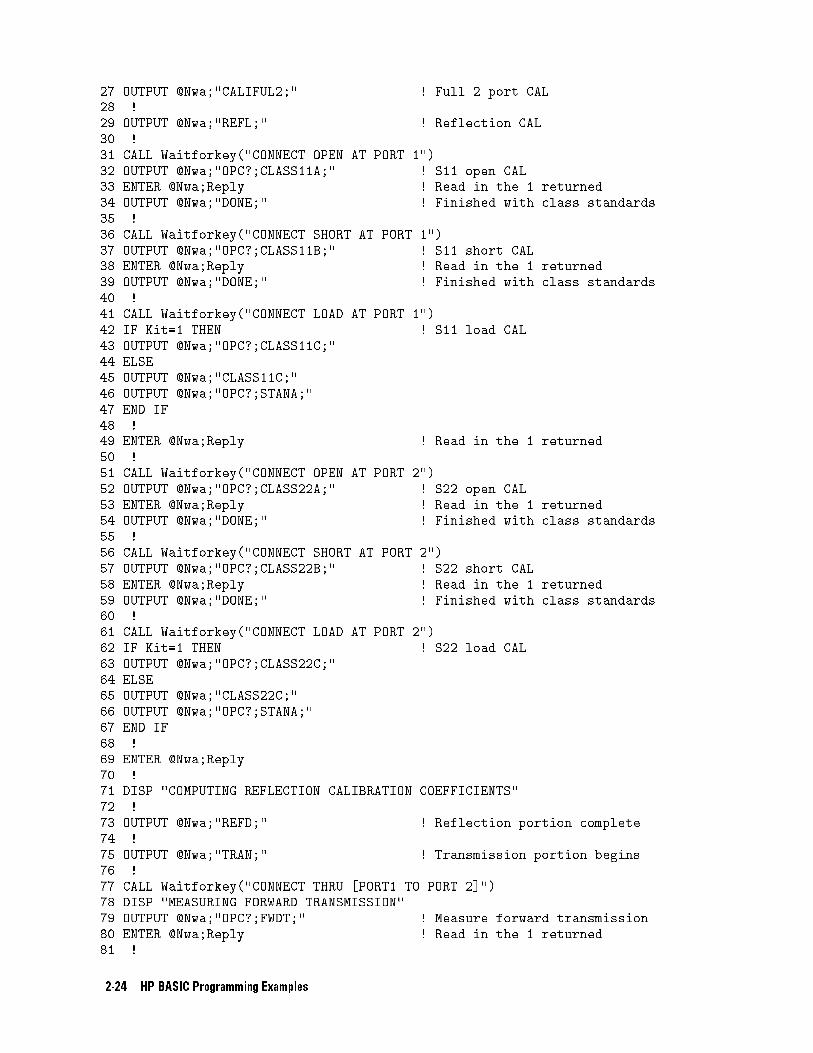
27 OUTPUT @Nwa;"CALIFUL2;" ! Full 2 port CAL
28 !
29 OUTPUT @Nwa;"REFL;" ! Reflection CAL
30 !
31 CALL Waitforkey("CONNECT OPEN AT PORT 1")
32 OUTPUT @Nwa;"OPC?;CLASS11A;" ! S11 open CAL
33 ENTER @Nwa;Reply ! Read in the 1 returned
34 OUTPUT @Nwa;"DONE;" ! Finished with class standards
35 !
36 CALL Waitforkey("CONNECT SHORT AT PORT 1")
37 OUTPUT @Nwa;"OPC?;CLASS11B;" ! S11 short CAL
38 ENTER @Nwa;Reply ! Read in the 1 returned
39 OUTPUT @Nwa;"DONE;" ! Finished with class standards
40 !
41 CALL Waitforkey("CONNECT LOAD AT PORT 1")
42 IF Kit=1 THEN ! S11 load CAL
43 OUTPUT @Nwa;"OPC?;CLASS11C;"
44 ELSE
45 OUTPUT @Nwa;"CLASS11C;"
46 OUTPUT @Nwa;"OPC?;STANA;"
47 END IF
48 !
49 ENTER @Nwa;Reply ! Read in the 1 returned
50 !
51 CALL Waitforkey("CONNECT OPEN AT PORT 2")
52 OUTPUT @Nwa;"OPC?;CLASS22A;" ! S22 open CAL
53 ENTER @Nwa;Reply ! Read in the 1 returned
54 OUTPUT @Nwa;"DONE;" ! Finished with class standards
55 !
56 CALL Waitforkey("CONNECT SHORT AT PORT 2")
57 OUTPUT @Nwa;"OPC?;CLASS22B;" ! S22 short CAL
58 ENTER @Nwa;Reply ! Read in the 1 returned
59 OUTPUT @Nwa;"DONE;" ! Finished with class standards
60 !
61 CALL Waitforkey("CONNECT LOAD AT PORT 2")
62 IF Kit=1 THEN ! S22 load CAL
63 OUTPUT @Nwa;"OPC?;CLASS22C;"
64 ELSE
65 OUTPUT @Nwa;"CLASS22C;"
66 OUTPUT @Nwa;"OPC?;STANA;"
67 END IF
68 !
69 ENTER @Nwa;Reply
70 !
71 DISP "COMPUTING REFLECTION CALIBRATION COEFFICIENTS"
72 !
73 OUTPUT @Nwa;"REFD;" ! Reflection portion complete
74 !
75 OUTPUT @Nwa;"TRAN;" ! Transmission portion begins
76 !
77 CALL Waitforkey("CONNECT THRU [PORT1 TO PORT 2]")
78 DISP "MEASURING FORWARD TRANSMISSION"
79 OUTPUT @Nwa;"OPC?;FWDT;" ! Measure forward transmission
80 ENTER @Nwa;Reply ! Read in the 1 returned
81 !
2-24 HP BASIC Programming Examples
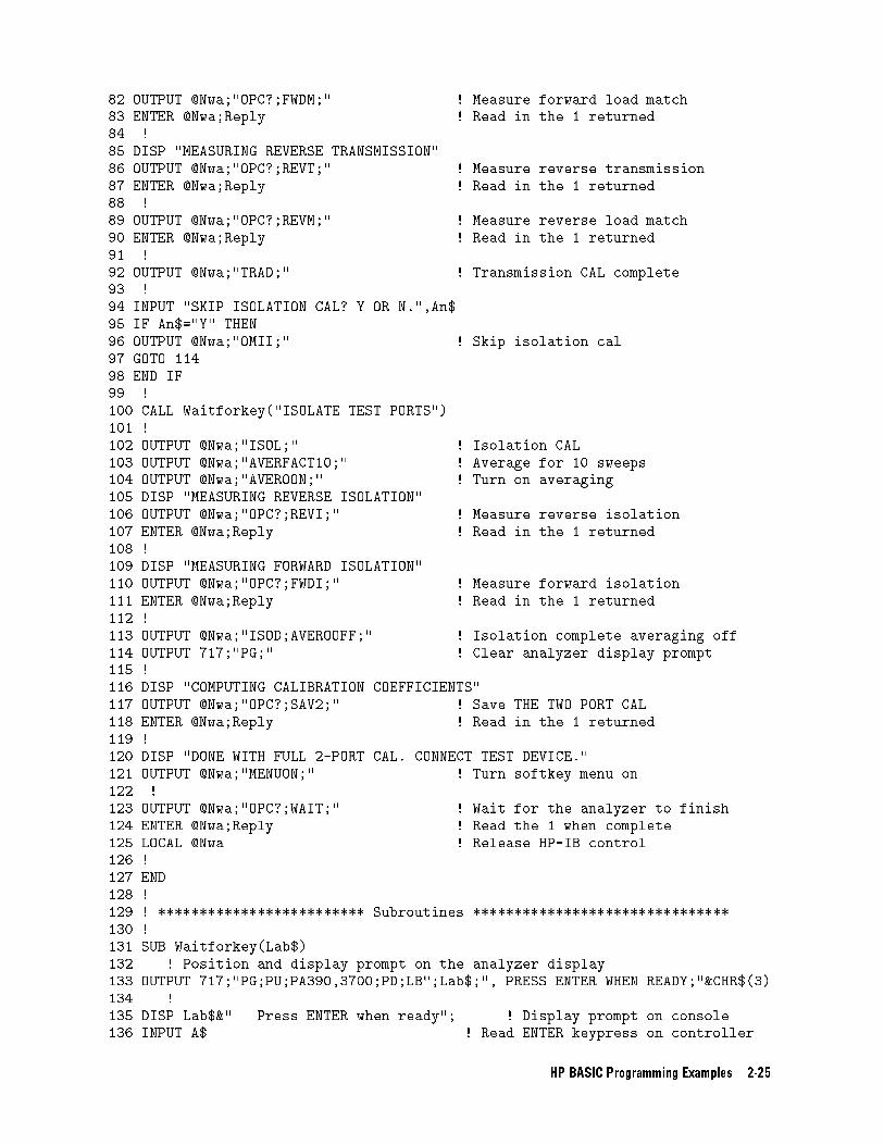
82 OUTPUT @Nwa;"OPC?;FWDM;" ! Measure forward load match
83 ENTER @Nwa;Reply ! Read in the 1 returned
84 !
85 DISP "MEASURING REVERSE TRANSMISSION"
86 OUTPUT @Nwa;"OPC?;REVT;" ! Measure reverse transmission
87 ENTER @Nwa;Reply ! Read in the 1 returned
88 !
89 OUTPUT @Nwa;"OPC?;REVM;" ! Measure reverse load match
90 ENTER @Nwa;Reply ! Read in the 1 returned
91 !
92 OUTPUT @Nwa;"TRAD;" ! Transmission CAL complete
93 !
94 INPUT "SKIP ISOLATION CAL? Y OR N.",An$
95 IF An$="Y" THEN
96 OUTPUT @Nwa;"OMII;" ! Skip isolation cal
97 GOTO 114
98 END IF
99 !
100 CALL Waitforkey("ISOLATE TEST PORTS")
101 !
102 OUTPUT @Nwa;"ISOL;" ! Isolation CAL
103 OUTPUT @Nwa;"AVERFACT10;" ! Average for 10 sweeps
104 OUTPUT @Nwa;"AVEROON;" ! Turn on averaging
105 DISP "MEASURING REVERSE ISOLATION"
106 OUTPUT @Nwa;"OPC?;REVI;" ! Measure reverse isolation
107 ENTER @Nwa;Reply ! Read in the 1 returned
108 !
109 DISP "MEASURING FORWARD ISOLATION"
110 OUTPUT @Nwa;"OPC?;FWDI;" ! Measure forward isolation
111 ENTER @Nwa;Reply ! Read in the 1 returned
112 !
113 OUTPUT @Nwa;"ISOD;AVEROOFF;" ! Isolation complete averaging off
114 OUTPUT 717;"PG;" ! Clear analyzer display prompt
115 !
116 DISP "COMPUTING CALIBRATION COEFFICIENTS"
117 OUTPUT @Nwa;"OPC?;SAV2;" ! Save THE TWO PORT CAL
118 ENTER @Nwa;Reply ! Read in the 1 returned
119 !
120 DISP "DONE WITH FULL 2-PORT CAL. CONNECT TEST DEVICE."
121 OUTPUT @Nwa;"MENUON;" ! Turn softkey menu on
122 !
123 OUTPUT @Nwa;"OPC?;WAIT;" ! Wait for the analyzer to finish
124 ENTER @Nwa;Reply ! Read the 1 when complete
125 LOCAL @Nwa ! Release HP-IB control
126 !
127 END
128 !
129 ! ************************* Subroutines *******************************
130 !
131 SUB Waitforkey(Lab$)
132 ! Position and display prompt on the analyzer display
133 OUTPUT 717;"PG;PU;PA390,3700;PD;LB";Lab$;", PRESS ENTER WHEN READY;"&CHR$(3)
134 !
135 DISP Lab$&" Press ENTER when ready"; ! Display prompt on console
136 INPUT A$ ! Read ENTER keypress on controller
HP BASIC Programming Examples 2-25
137 OUTPUT 717;"PG;" ! Clear analyzer display
138 SUBEND
Running the Program
Note Before running the program, set the desired instrument state. This program
does not modify the instrument state in any way.
Run the program and connect the standards as prompted. After the standard is connected,
press �ENTER� on the controller keyboard to continue the program.
The program assumes that the test ports have either a 7-mm or 3.5-mm interface or an adapter
set using either a 7-mm or 3.5-mm interface. The prompts appear just above the message
line on the analyzer display. After the prompt is displayed, pressing �ENTER� on the computer
console continues the program and measures the standard. The operator has the option
of omitting the isolation calibration. If the isolation calibration is performed, averaging is
automatically employed to insure a good calibration. The program will display a message when
the measurement calibration is complete.
2-26 HP BASIC Programming Examples
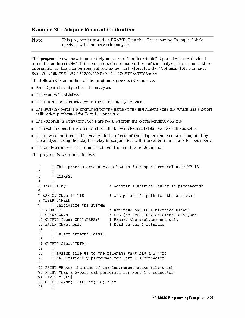
Example 2C: Adapter Removal Calibration
Note This program is stored as EXAMP2C on the \Programming Examples" disk
received with the network analyzer.
This program shows how to accurately measure a \non-insertable" 2-port device. A device is
termed \non-insertable" if its connectors do not match those of the analyzer front panel. More
information on the adapter removal technique can be found in the \Optimizing Measurement
Results" chapter of the HP 8753D Network Analyzer User's Guide.
The following is an outline of the program's processing sequence:
An I/O path is assigned for the analyzer.
The system is initialized.
The internal disk is selected as the active storage device.
The system operator is prompted for the name of the instrument state �le which has a 2-port
calibration performed for Port 1's connector.
The calibration arrays for Port 1 are recalled from the corresponding disk �le.
The system operator is prompted for the known electrical delay value of the adapter.
The new calibration coe�cients, with the e�ects of the adapter removed, are computed by
the analyzer using the adapter delay in conjunction with the calibration arrays for both ports.
The analyzer is released from remote control and the program ends.
The program is written as follows:
1 ! This program demonstrates how to do adapter removal over HP-IB.
2 !
3 ! EXAMP2C
4 !
5 REAL Delay ! Adapter electrical delay in picoseconds
6 !
7 ASSIGN @Nwa TO 716 ! Assign an I/O path for the analyzer
8 CLEAR SCREEN
9 ! Initialize the system
10 ABORT 7 ! Generate an IFC (Interface Clear)
11 CLEAR @Nwa ! SDC (Selected Device Clear) analyzer
12 OUTPUT @Nwa;"OPC?;PRES;" ! Preset the analyzer and wait
13 ENTER @Nwa;Reply ! Read in the 1 returned
14 !
15 ! Select internal disk.
16 !
17 OUTPUT @Nwa;"INTD;"
18 !
19 ! Assign file #1 to the filename that has a 2-port
20 ! cal previously performed for Port 1's connector.
21 !
22 PRINT "Enter the name of the instrument state file which"
23 PRINT "has a 2-port cal performed for Port 1's connector"
24 INPUT "",F1$
25 OUTPUT @Nwa;"TITF1""";F1$;""";"
26 !
HP BASIC Programming Examples 2-27
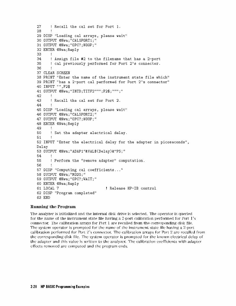
27 ! Recall the cal set for Port 1.
28 !
29 DISP "Loading cal arrays, please wait"
30 OUTPUT @Nwa;"CALSPORT1;"
31 OUTPUT @Nwa;"OPC?;NOOP;"
32 ENTER @Nwa;Reply
33 !
34 ! Assign file #2 to the filename that has a 2-port
35 ! cal previously performed for Port 2's connector.
36 !
37 CLEAR SCREEN
38 PRINT "Enter the name of the instrument state file which"
39 PRINT "has a 2-port cal performed for Port 2's connector"
40 INPUT "",F2$
41 OUTPUT @Nwa;"INTD;TITF2""";F2$;""";"
42 !
43 ! Recall the cal set for Port 2.
44 !
45 DISP "Loading cal arrays, please wait"
46 OUTPUT @Nwa;"CALSPORT2;"
47 OUTPUT @Nwa;"OPC?;NOOP;"
48 ENTER @Nwa;Reply
49 !
50 ! Set the adapter electrical delay.
51 !
52 INPUT "Enter the electrical delay for the adapter in picoseconds",
Delay
53 OUTPUT @Nwa;"ADAP1"&VAL$(Delay)&"PS;"
54 !
55 ! Perform the "remove adapter" computation.
56 !
57 DISP "Computing cal coefficients..."
58 OUTPUT @Nwa;"MODS;"
59 OUTPUT @Nwa;"OPC?;WAIT;"
60 ENTER @Nwa;Reply
61 LOCAL 7 ! Release HP-IB control
62 DISP "Program completed"
63 END
Running the Program
The analyzer is initialized and the internal disk drive is selected. The operator is queried
for the name of the instrument state �le having a 2-port calibration performed for Port 1's
connector. The calibration arrays for Port 1 are recalled from the corresponding disk �le.
The system operator is prompted for the name of the instrument state �le having a 2-port
calibration performed for Port 2's connector. The calibration arrays for Port 2 are recalled from
the corresponding disk �le. The system operator is prompted for the known electrical delay of
the adapter and this value is written to the analyzer. The calibration coe�cients with adapter
e�ects removed are computed and the program ends.
2-28 HP BASIC Programming Examples
Example 2D: Using Raw Data to Create a Calibration (Simmcal)
Note This program is stored as EXAMP2D on the \Programming Examples" disk
received with the network analyzer.
This program simulates a full 2-port cal by measuring the raw data for each \standard" and
then loading it later into the appropriate arrays. The program can be adapted to create
additional calibrations using the same arrays. It uses the HP85031B 7-mm cal kit.
Caution This feature is not currently supported with TRL calibrations.
The following is an outline of the programs' processing sequence:
An I/O path is assigned for the analyzer.
The system is initiated.
The number of points is set to correspond to the size of the dimensioned memory arrays and
ASCII data format is selected.
The 7-mm calibration kit is selected, sweep time is set to 1 second, and the analyzer is placed
into hold mode.
S11 measurement is selected for gathering the forward re ection standards.
The system operator is prompted to connect each of the three standards, one at a time.
Following each prompt, a single sweep is taken and the raw measured data for that standard
is read from the analyzer into a corresponding memory array in the controller.
S22 measurement is selected for gathering the reverse re ection standards.
The system operator is prompted in the same manner as before and the raw data for the
three standards is measured and stored away as before.
The system operator is prompted to make the thru connection between Port 1 and Port 2.
S21 measurement is selected, a single sweep is taken and the raw data is read into an array
corresponding to forward transmission.
S11 measurement is selected, a single sweep is taken and the raw data is read into an array
corresponding to forward thru match.
S12 measurement is selected, a single sweep is taken and the raw data is read into an array
corresponding to reverse transmission.
S22 measurement is selected, a single sweep is taken and the raw data is read into an array
corresponding to reverse thru match.
The analyzer begins the normal 2-port calibration procedure, but with the default beep
turned o�.
A single sweep is taken for the measurement of each standard to provide \dummy" data,
which is immediately replaced with the previously measured raw data from the array
corresponding to that measurement.
The analyzer uses the raw data to compute the error coe�cients and is placed back into
continuous sweep mode.
The analyzer is released from remote control and the program ends.
HP BASIC Programming Examples 2-29
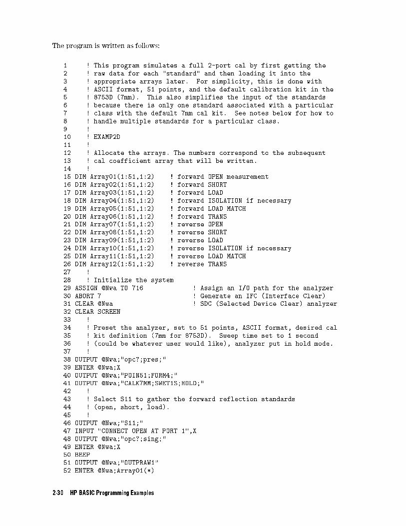
The program is written as follows:
1 ! This program simulates a full 2-port cal by first getting the
2 ! raw data for each "standard" and then loading it into the
3 ! appropriate arrays later. For simplicity, this is done with
4 ! ASCII format, 51 points, and the default calibration kit in the
5 ! 8753D (7mm). This also simplifies the input of the standards
6 ! because there is only one standard associated with a particular
7 ! class with the default 7mm cal kit. See notes below for how to
8 ! handle multiple standards for a particular class.
9 !
10 ! EXAMP2D
11 !
12 ! Allocate the arrays. The numbers correspond to the subsequent
13 ! cal coefficient array that will be written.
14 !
15 DIM Array01(1:51,1:2) ! forward OPEN measurement
16 DIM Array02(1:51,1:2) ! forward SHORT
17 DIM Array03(1:51,1:2) ! forward LOAD
18 DIM Array04(1:51,1:2) ! forward ISOLATION if necessary
19 DIM Array05(1:51,1:2) ! forward LOAD MATCH
20 DIM Array06(1:51,1:2) ! forward TRANS
21 DIM Array07(1:51,1:2) ! reverse OPEN
22 DIM Array08(1:51,1:2) ! reverse SHORT
23 DIM Array09(1:51,1:2) ! reverse LOAD
24 DIM Array10(1:51,1:2) ! reverse ISOLATION if necessary
25 DIM Array11(1:51,1:2) ! reverse LOAD MATCH
26 DIM Array12(1:51,1:2) ! reverse TRANS
27 !
28 ! Initialize the system
29 ASSIGN @Nwa TO 716 ! Assign an I/O path for the analyzer
30 ABORT 7 ! Generate an IFC (Interface Clear)
31 CLEAR @Nwa ! SDC (Selected Device Clear) analyzer
32 CLEAR SCREEN
33 !
34 ! Preset the analyzer, set to 51 points, ASCII format, desired cal
35 ! kit definition (7mm for 8753D). Sweep time set to 1 second
36 ! (could be whatever user would like), analyzer put in hold mode.
37 !
38 OUTPUT @Nwa;"opc?;pres;"
39 ENTER @Nwa;X
40 OUTPUT @Nwa;"POIN51;FORM4;"
41 OUTPUT @Nwa;"CALK7MM;SWET1S;HOLD;"
42 !
43 ! Select S11 to gather the forward reflection standards
44 ! (open, short, load).
45 !
46 OUTPUT @Nwa;"S11;"
47 INPUT "CONNECT OPEN AT PORT 1",X
48 OUTPUT @Nwa;"opc?;sing;"
49 ENTER @Nwa;X
50 BEEP
51 OUTPUT @Nwa;"OUTPRAW1"
52 ENTER @Nwa;Array01(*)
2-30 HP BASIC Programming Examples
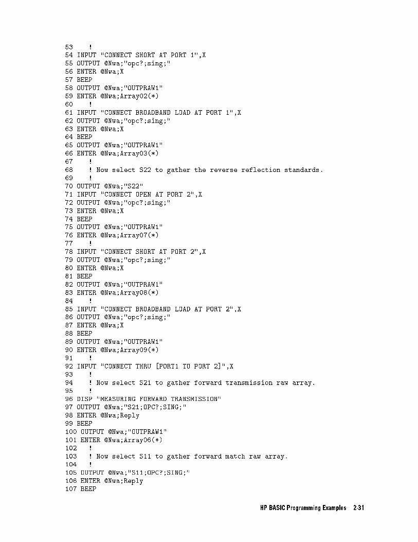
53 !
54 INPUT "CONNECT SHORT AT PORT 1",X
55 OUTPUT @Nwa;"opc?;sing;"
56 ENTER @Nwa;X
57 BEEP
58 OUTPUT @Nwa;"OUTPRAW1"
59 ENTER @Nwa;Array02(*)
60 !
61 INPUT "CONNECT BROADBAND LOAD AT PORT 1",X
62 OUTPUT @Nwa;"opc?;sing;"
63 ENTER @Nwa;X
64 BEEP
65 OUTPUT @Nwa;"OUTPRAW1"
66 ENTER @Nwa;Array03(*)
67 !
68 ! Now select S22 to gather the reverse reflection standards.
69 !
70 OUTPUT @Nwa;"S22"
71 INPUT "CONNECT OPEN AT PORT 2",X
72 OUTPUT @Nwa;"opc?;sing;"
73 ENTER @Nwa;X
74 BEEP
75 OUTPUT @Nwa;"OUTPRAW1"
76 ENTER @Nwa;Array07(*)
77 !
78 INPUT "CONNECT SHORT AT PORT 2",X
79 OUTPUT @Nwa;"opc?;sing;"
80 ENTER @Nwa;X
81 BEEP
82 OUTPUT @Nwa;"OUTPRAW1"
83 ENTER @Nwa;Array08(*)
84 !
85 INPUT "CONNECT BROADBAND LOAD AT PORT 2",X
86 OUTPUT @Nwa;"opc?;sing;"
87 ENTER @Nwa;X
88 BEEP
89 OUTPUT @Nwa;"OUTPRAW1"
90 ENTER @Nwa;Array09(*)
91 !
92 INPUT "CONNECT THRU [PORT1 TO PORT 2]",X
93 !
94 ! Now select S21 to gather forward transmission raw array.
95 !
96 DISP "MEASURING FORWARD TRANSMISSION"
97 OUTPUT @Nwa;"S21;OPC?;SING;"
98 ENTER @Nwa;Reply
99 BEEP
100 OUTPUT @Nwa;"OUTPRAW1"
101 ENTER @Nwa;Array06(*)
102 !
103 ! Now select S11 to gather forward match raw array.
104 !
105 OUTPUT @Nwa;"S11;OPC?;SING;"
106 ENTER @Nwa;Reply
107 BEEP
HP BASIC Programming Examples 2-31
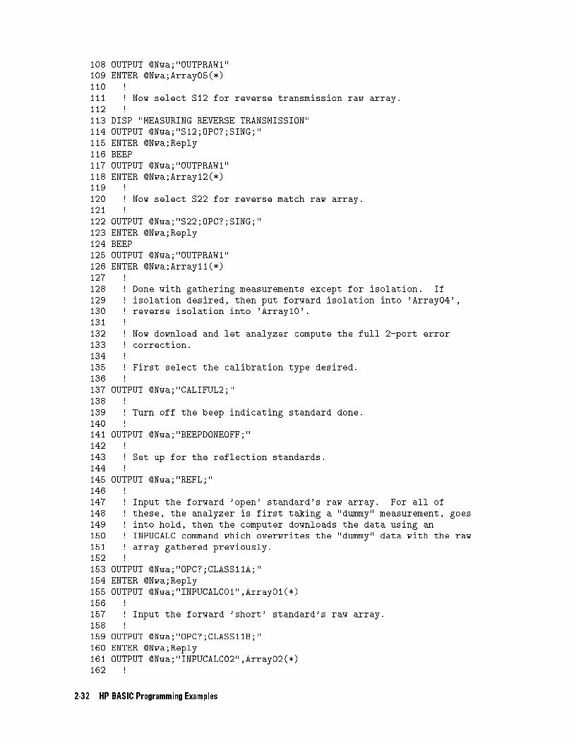
108 OUTPUT @Nwa;"OUTPRAW1"
109 ENTER @Nwa;Array05(*)
110 !
111 ! Now select S12 for reverse transmission raw array.
112 !
113 DISP "MEASURING REVERSE TRANSMISSION"
114 OUTPUT @Nwa;"S12;OPC?;SING;"
115 ENTER @Nwa;Reply
116 BEEP
117 OUTPUT @Nwa;"OUTPRAW1"
118 ENTER @Nwa;Array12(*)
119 !
120 ! Now select S22 for reverse match raw array.
121 !
122 OUTPUT @Nwa;"S22;OPC?;SING;"
123 ENTER @Nwa;Reply
124 BEEP
125 OUTPUT @Nwa;"OUTPRAW1"
126 ENTER @Nwa;Array11(*)
127 !
128 ! Done with gathering measurements except for isolation. If
129 ! isolation desired, then put forward isolation into 'Array04',
130 ! reverse isolation into 'Array10'.
131 !
132 ! Now download and let analyzer compute the full 2-port error
133 ! correction.
134 !
135 ! First select the calibration type desired.
136 !
137 OUTPUT @Nwa;"CALIFUL2;"
138 !
139 ! Turn off the beep indicating standard done.
140 !
141 OUTPUT @Nwa;"BEEPDONEOFF;"
142 !
143 ! Set up for the reflection standards.
144 !
145 OUTPUT @Nwa;"REFL;"
146 !
147 ! Input the forward 'open' standard's raw array. For all of
148 ! these, the analyzer is first taking a "dummy" measurement, goes
149 ! into hold, then the computer downloads the data using an
150 ! INPUCALC command which overwrites the "dummy" data with the raw
151 ! array gathered previously.
152 !
153 OUTPUT @Nwa;"OPC?;CLASS11A;"
154 ENTER @Nwa;Reply
155 OUTPUT @Nwa;"INPUCALC01",Array01(*)
156 !
157 ! Input the forward 'short' standard's raw array.
158 !
159 OUTPUT @Nwa;"OPC?;CLASS11B;"
160 ENTER @Nwa;Reply
161 OUTPUT @Nwa;"INPUCALC02",Array02(*)
162 !
2-32 HP BASIC Programming Examples
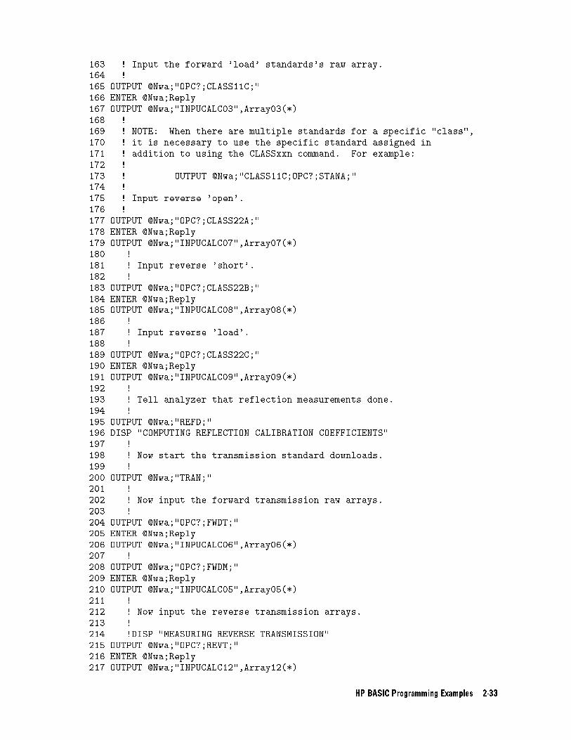
163 ! Input the forward 'load' standards's raw array.
164 !
165 OUTPUT @Nwa;"OPC?;CLASS11C;"
166 ENTER @Nwa;Reply
167 OUTPUT @Nwa;"INPUCALC03",Array03(*)
168 !
169 ! NOTE: When there are multiple standards for a specific "class",
170 ! it is necessary to use the specific standard assigned in
171 ! addition to using the CLASSxxn command. For example:
172 !
173 ! OUTPUT @Nwa;"CLASS11C;OPC?;STANA;"
174 !
175 ! Input reverse 'open'.
176 !
177 OUTPUT @Nwa;"OPC?;CLASS22A;"
178 ENTER @Nwa;Reply
179 OUTPUT @Nwa;"INPUCALC07",Array07(*)
180 !
181 ! Input reverse 'short'.
182 !
183 OUTPUT @Nwa;"OPC?;CLASS22B;"
184 ENTER @Nwa;Reply
185 OUTPUT @Nwa;"INPUCALC08",Array08(*)
186 !
187 ! Input reverse 'load'.
188 !
189 OUTPUT @Nwa;"OPC?;CLASS22C;"
190 ENTER @Nwa;Reply
191 OUTPUT @Nwa;"INPUCALC09",Array09(*)
192 !
193 ! Tell analyzer that reflection measurements done.
194 !
195 OUTPUT @Nwa;"REFD;"
196 DISP "COMPUTING REFLECTION CALIBRATION COEFFICIENTS"
197 !
198 ! Now start the transmission standard downloads.
199 !
200 OUTPUT @Nwa;"TRAN;"
201 !
202 ! Now input the forward transmission raw arrays.
203 !
204 OUTPUT @Nwa;"OPC?;FWDT;"
205 ENTER @Nwa;Reply
206 OUTPUT @Nwa;"INPUCALC06",Array06(*)
207 !
208 OUTPUT @Nwa;"OPC?;FWDM;"
209 ENTER @Nwa;Reply
210 OUTPUT @Nwa;"INPUCALC05",Array05(*)
211 !
212 ! Now input the reverse transmission arrays.
213 !
214 !DISP "MEASURING REVERSE TRANSMISSION"
215 OUTPUT @Nwa;"OPC?;REVT;"
216 ENTER @Nwa;Reply
217 OUTPUT @Nwa;"INPUCALC12",Array12(*)
HP BASIC Programming Examples 2-33
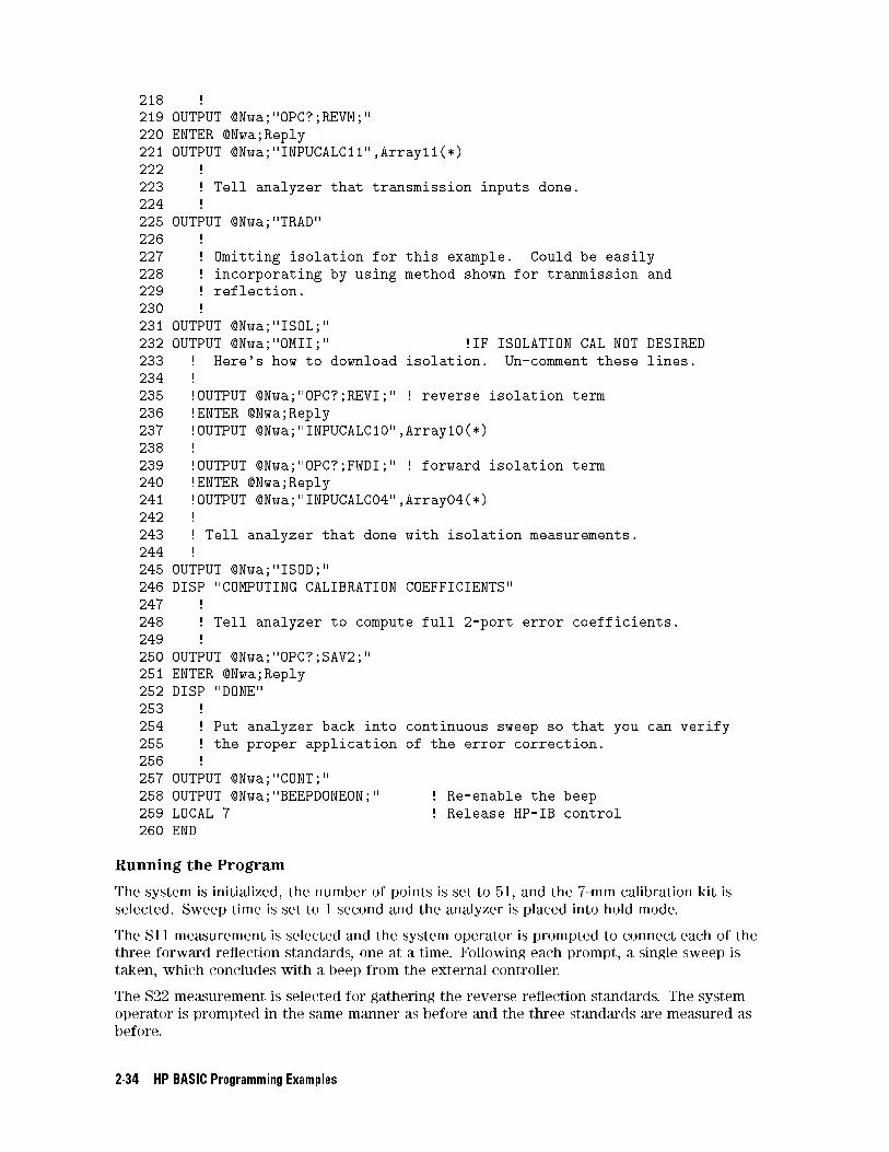
218 !
219 OUTPUT @Nwa;"OPC?;REVM;"
220 ENTER @Nwa;Reply
221 OUTPUT @Nwa;"INPUCALC11",Array11(*)
222 !
223 ! Tell analyzer that transmission inputs done.
224 !
225 OUTPUT @Nwa;"TRAD"
226 !
227 ! Omitting isolation for this example. Could be easily
228 ! incorporating by using method shown for tranmission and
229 ! reflection.
230 !
231 OUTPUT @Nwa;"ISOL;"
232 OUTPUT @Nwa;"OMII;" !IF ISOLATION CAL NOT DESIRED
233 ! Here's how to download isolation. Un-comment these lines.
234 !
235 !OUTPUT @Nwa;"OPC?;REVI;" ! reverse isolation term
236 !ENTER @Nwa;Reply
237 !OUTPUT @Nwa;"INPUCALC10",Array10(*)
238 !
239 !OUTPUT @Nwa;"OPC?;FWDI;" ! forward isolation term
240 !ENTER @Nwa;Reply
241 !OUTPUT @Nwa;"INPUCALC04",Array04(*)
242 !
243 ! Tell analyzer that done with isolation measurements.
244 !
245 OUTPUT @Nwa;"ISOD;"
246 DISP "COMPUTING CALIBRATION COEFFICIENTS"
247 !
248 ! Tell analyzer to compute full 2-port error coefficients.
249 !
250 OUTPUT @Nwa;"OPC?;SAV2;"
251 ENTER @Nwa;Reply
252 DISP "DONE"
253 !
254 ! Put analyzer back into continuous sweep so that you can verify
255 ! the proper application of the error correction.
256 !
257 OUTPUT @Nwa;"CONT;"
258 OUTPUT @Nwa;"BEEPDONEON;" ! Re-enable the beep
259 LOCAL 7 ! Release HP-IB control
260 END
Running the Program
The system is initialized, the number of points is set to 51, and the 7-mm calibration kit is
selected. Sweep time is set to 1 second and the analyzer is placed into hold mode.
The S11 measurement is selected and the system operator is prompted to connect each of the
three forward re ection standards, one at a time. Following each prompt, a single sweep is
taken, which concludes with a beep from the external controller.
The S22 measurement is selected for gathering the reverse re ection standards. The system
operator is prompted in the same manner as before and the three standards are measured as
before.
2-34 HP BASIC Programming Examples

The system operator is prompted to make the thru connection between Port 1 and Port 2. A
single sweep is taken for each of the four S-parameters, each concluding with a beep.
The analyzer begins the normal 2-port calibration procedure, but with the default beep turned
o�. A single sweep is taken for each measurement of each standard, providing \dummy"
data which is immediately replaced with the data from the array corresponding to that
measurement. The analyzer computes the error correction coe�cients and is placed back into
continuous sweep mode. The default beep is re-enabled and the program ends.
HP BASIC Programming Examples 2-35
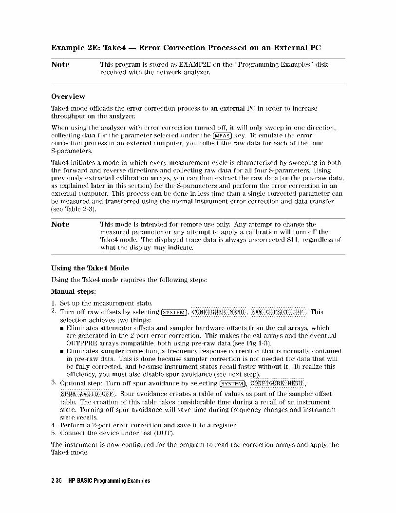
Example 2E: Take4 | Error Correction Processed on an External PC
Note This program is stored as EXAMP2E on the \Programming Examples" disk
received with the network analyzer.
Overview
Take4 mode o�oads the error correction process to an external PC in order to increase
throughput on the analyzer.
When using the analyzer with error correction turned o�, it will only sweep in one direction,
collecting data for the parameter selected under the �MEAS� key. To emulate the errorcorrection process in an external computer, you collect the raw data for each of the four
S-parameters.
Take4 initiates a mode in which every measurement cycle is characterized by sweeping in both
the forward and reverse directions and collecting raw data for all four S-parameters. Using
previously extracted calibration arrays, you can then extract the raw data (or the pre-raw data,
as explained later in this section) for the S-parameters and perform the error correction in an
external computer. This process can be done in less time than a single corrected parameter can
be measured and transferred using the normal instrument error correction and data transfer
(see Table 2-3).
Note This mode is intended for remote use only. Any attempt to change the
measured parameter or any attempt to apply a calibration will turn o� the
Take4 mode. The displayed trace data is always uncorrected S11, regardless of
what the display may indicate.
Using the Take4 Mode
Using the Take4 mode requires the following steps:
Manual steps:
1. Set up the measurement state.
2. Turn o� raw o�sets by selecting �SYSTEM�,NNNNNNNNNNNNNNNNNNNNNNNNNNNNNNNNNNNNNNNNNNNNCONFIGURE MENU ,
NNNNNNNNNNNNNNNNNNNNNNNNNNNNNNNNNNNNNNNNNNNNRAW OFFSET OFF . This
selection achieves two things:
Eliminates attenuator o�sets and sampler hardware o�sets from the cal arrays, which
are generated in the 2-port error correction. This makes the cal arrays and the eventual
OUTPPRE arrays compatible, both using pre-raw data (see Fig 1-3).
Eliminates sampler correction, a frequency response correction that is normally contained
in pre-raw data. This is done because sampler correction is not needed for data that will
be fully corrected, and because instrument states recall faster without it. To realize this
e�ciency, you must also disable spur avoidance (see next step).
3. Optional step: Turn o� spur avoidance by selecting �SYSTEM�,NNNNNNNNNNNNNNNNNNNNNNNNNNNNNNNNNNNNNNNNNNNNCONFIGURE MENU ,
NNNNNNNNNNNNNNNNNNNNNNNNNNNNNNNNNNNNNNNNNNNNSPUR AVOID OFF . Spur avoidance creates a table of values as part of the sampler o�set
table. The creation of this table takes considerable time during a recall of an instrument
state. Turning o� spur avoidance will save time during frequency changes and instrument
state recalls.
4. Perform a 2-port error correction and save it to a register.
5. Connect the device under test (DUT).
The instrument is now con�gured for the program to read the correction arrays and apply the
Take4 mode.
2-36 HP BASIC Programming Examples
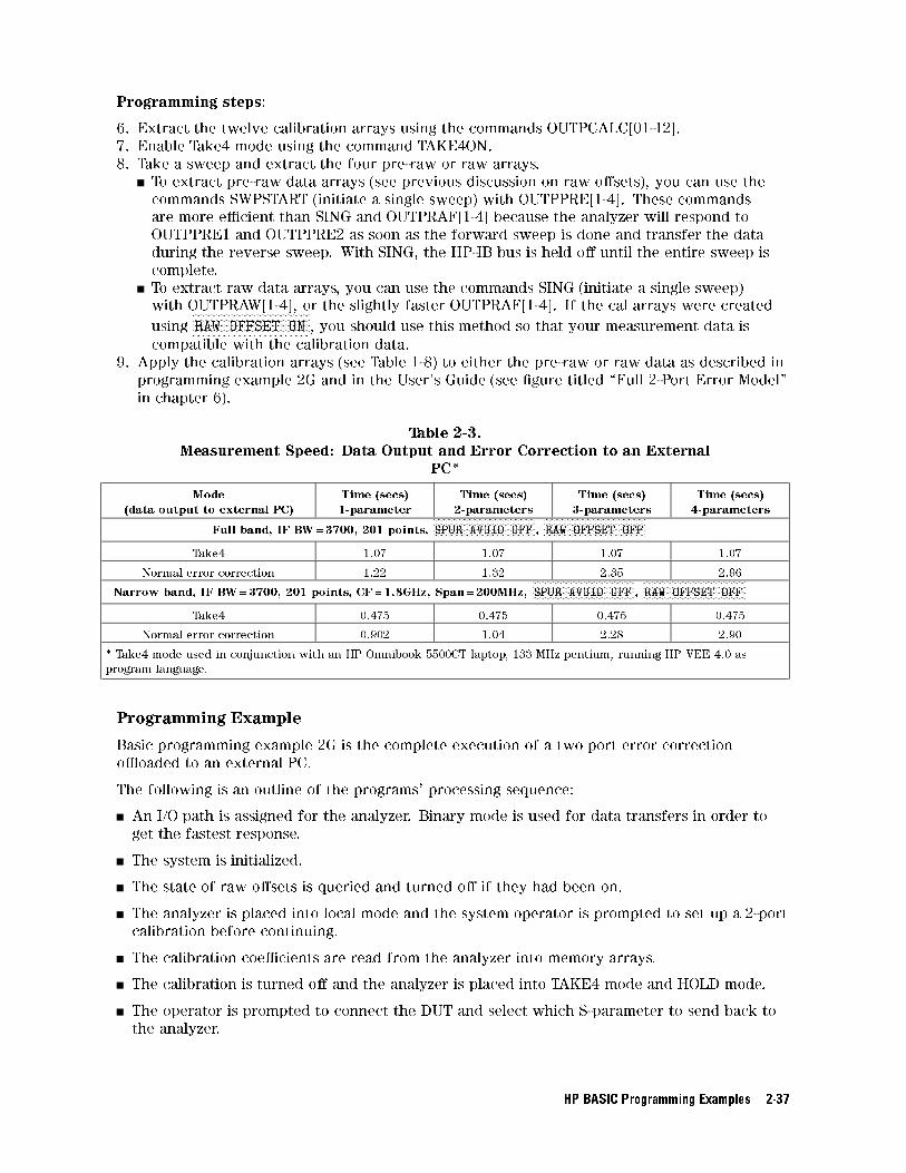
Programming steps:
6. Extract the twelve calibration arrays using the commands OUTPCALC[01-12].
7. Enable Take4 mode using the command TAKE4ON.
8. Take a sweep and extract the four pre-raw or raw arrays.
To extract pre-raw data arrays (see previous discussion on raw o�sets), you can use the
commands SWPSTART (initiate a single sweep) with OUTPPRE[1-4]. These commands
are more e�cient than SING and OUTPRAF[1-4] because the analyzer will respond to
OUTPPRE1 and OUTPPRE2 as soon as the forward sweep is done and transfer the data
during the reverse sweep. With SING, the HP-IB bus is held o� until the entire sweep is
complete.
To extract raw data arrays, you can use the commands SING (initiate a single sweep)
with OUTPRAW[1-4], or the slightly faster OUTPRAF[1-4]. If the cal arrays were created
usingNNNNNNNNNNNNNNNNNNNNNNNNNNNNNNNNNNNNNNNNNRAW OFFSET ON , you should use this method so that your measurement data is
compatible with the calibration data.
9. Apply the calibration arrays (see Table 1-8) to either the pre-raw or raw data as described in
programming example 2G and in the User's Guide (see �gure titled \Full 2-Port Error Model"
in chapter 6).
Table 2-3.Measurement Speed: Data Output and Error Correction to an External
PC*
Mode
(data output to external PC)
Time (secs)
1-parameter
Time (secs)
2-parameters
Time (secs)
3-parameters
Time (secs)
4-parameters
Full band, IF BW=3700, 201 points,FFFFFFFFFFFFFFFFFFFFFFFFFFFFFFFFFFFFSPUR AVOID OFF ,
FFFFFFFFFFFFFFFFFFFFFFFFFFFFFFFFFFFFRAW OFFSET OFF
Take4 1.07 1.07 1.07 1.07
Normal error correction 1.22 1.32 2.35 2.96
Narrow band, IF BW=3700, 201 points, CF=1.8GHz, Span=200MHz,FFFFFFFFFFFFFFFFFFFFFFFFFFFFFFFFFFFFSPUR AVOID OFF ,
FFFFFFFFFFFFFFFFFFFFFFFFFFFFFFFFFFFFRAW OFFSET OFF
Take4 0.475 0.475 0.475 0.475
Normal error correction 0.902 1.04 2.28 2.90
* Take4 mode used in conjunction with an HP Omnibook 5500CT laptop, 133 MHz pentium, running HP VEE 4.0 as
program language.
Programming Example
Basic programming example 2G is the complete execution of a two port error correction
o�oaded to an external PC.
The following is an outline of the programs' processing sequence:
An I/O path is assigned for the analyzer. Binary mode is used for data transfers in order to
get the fastest response.
The system is initialized.
The state of raw o�sets is queried and turned o� if they had been on.
The analyzer is placed into local mode and the system operator is prompted to set up a 2-port
calibration before continuing.
The calibration coe�cients are read from the analyzer into memory arrays.
The calibration is turned o� and the analyzer is placed into TAKE4 mode and HOLD mode.
The operator is prompted to connect the DUT and select which S-parameter to send back to
the analyzer.
HP BASIC Programming Examples 2-37
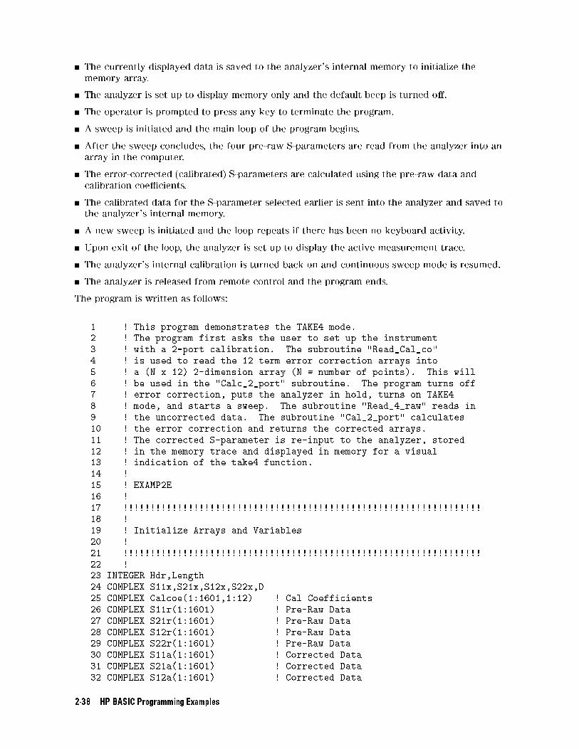
The currently displayed data is saved to the analyzer's internal memory to initialize the
memory array.
The analyzer is set up to display memory only and the default beep is turned o�.
The operator is prompted to press any key to terminate the program.
A sweep is initiated and the main loop of the program begins.
After the sweep concludes, the four pre-raw S-parameters are read from the analyzer into an
array in the computer.
The error-corrected (calibrated) S-parameters are calculated using the pre-raw data and
calibration coe�cients.
The calibrated data for the S-parameter selected earlier is sent into the analyzer and saved to
the analyzer's internal memory.
A new sweep is initiated and the loop repeats if there has been no keyboard activity.
Upon exit of the loop, the analyzer is set up to display the active measurement trace.
The analyzer's internal calibration is turned back on and continuous sweep mode is resumed.
The analyzer is released from remote control and the program ends.
The program is written as follows:
1 ! This program demonstrates the TAKE4 mode.
2 ! The program first asks the user to set up the instrument
3 ! with a 2-port calibration. The subroutine "Read_Cal_co"
4 ! is used to read the 12 term error correction arrays into
5 ! a (N x 12) 2-dimension array (N = number of points). This will
6 ! be used in the "Calc_2_port" subroutine. The program turns off
7 ! error correction, puts the analyzer in hold, turns on TAKE4
8 ! mode, and starts a sweep. The subroutine "Read_4_raw" reads in
9 ! the uncorrected data. The subroutine "Cal_2_port" calculates
10 ! the error correction and returns the corrected arrays.
11 ! The corrected S-parameter is re-input to the analyzer, stored
12 ! in the memory trace and displayed in memory for a visual
13 ! indication of the take4 function.
14 !
15 ! EXAMP2E
16 !
17 !!!!!!!!!!!!!!!!!!!!!!!!!!!!!!!!!!!!!!!!!!!!!!!!!!!!!!!!!!!!!!!!!!
18 !
19 ! Initialize Arrays and Variables
20 !
21 !!!!!!!!!!!!!!!!!!!!!!!!!!!!!!!!!!!!!!!!!!!!!!!!!!!!!!!!!!!!!!!!!!
22 !
23 INTEGER Hdr,Length
24 COMPLEX S11x,S21x,S12x,S22x,D
25 COMPLEX Calcoe(1:1601,1:12) ! Cal Coefficients
26 COMPLEX S11r(1:1601) ! Pre-Raw Data
27 COMPLEX S21r(1:1601) ! Pre-Raw Data
28 COMPLEX S12r(1:1601) ! Pre-Raw Data
29 COMPLEX S22r(1:1601) ! Pre-Raw Data
30 COMPLEX S11a(1:1601) ! Corrected Data
31 COMPLEX S21a(1:1601) ! Corrected Data
32 COMPLEX S12a(1:1601) ! Corrected Data
2-38 HP BASIC Programming Examples
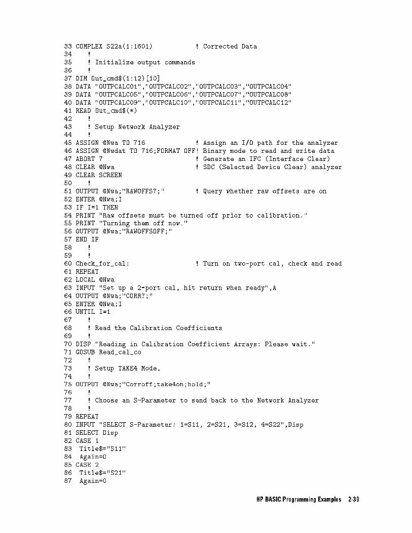
33 COMPLEX S22a(1:1601) ! Corrected Data
34 !
35 ! Initialize output commands
36 !
37 DIM Out_cmd$(1:12)[10]
38 DATA "OUTPCALC01","OUTPCALC02","OUTPCALC03","OUTPCALC04"
39 DATA "OUTPCALC05","OUTPCALC06","OUTPCALC07","OUTPCALC08"
40 DATA "OUTPCALC09","OUTPCALC10","OUTPCALC11","OUTPCALC12"
41 READ Out_cmd$(*)
42 !
43 ! Setup Network Analyzer
44 !
45 ASSIGN @Nwa TO 716 ! Assign an I/O path for the analyzer
46 ASSIGN @Nwdat TO 716;FORMAT OFF! Binary mode to read and write data
47 ABORT 7 ! Generate an IFC (Interface Clear)
48 CLEAR @Nwa ! SDC (Selected Device Clear) analyzer
49 CLEAR SCREEN
50 !
51 OUTPUT @Nwa;"RAWOFFS?;" ! Query whether raw offsets are on
52 ENTER @Nwa;I
53 IF I=1 THEN
54 PRINT "Raw offsets must be turned off prior to calibration."
55 PRINT "Turning them off now."
56 OUTPUT @Nwa;"RAWOFFSOFF;"
57 END IF
58 !
59 !
60 Check_for_cal: ! Turn on two-port cal, check and read
61 REPEAT
62 LOCAL @Nwa
63 INPUT "Set up a 2-port cal, hit return when ready",A
64 OUTPUT @Nwa;"CORR?;"
65 ENTER @Nwa;I
66 UNTIL I=1
67 !
68 ! Read the Calibration Coefficients
69 !
70 DISP "Reading in Calibration Coefficient Arrays: Please wait."
71 GOSUB Read_cal_co
72 !
73 ! Setup TAKE4 Mode,
74 !
75 OUTPUT @Nwa;"Corroff;take4on;hold;"
76 !
77 ! Choose an S-Parameter to send back to the Network Analyzer
78 !
79 REPEAT
80 INPUT "SELECT S-Parameter: 1=S11, 2=S21, 3=S12, 4=S22",Disp
81 SELECT Disp
82 CASE 1
83 Title$="S11"
84 Again=0
85 CASE 2
86 Title$="S21"
87 Again=0
HP BASIC Programming Examples 2-39
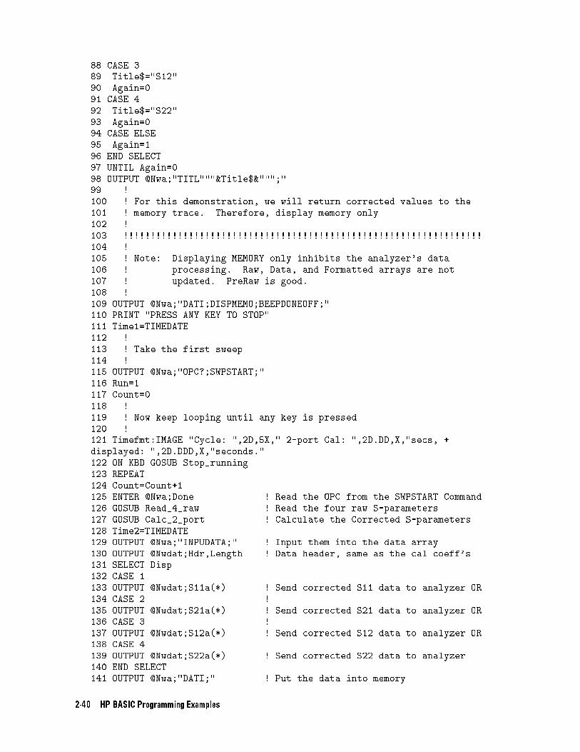
88 CASE 3
89 Title$="S12"
90 Again=0
91 CASE 4
92 Title$="S22"
93 Again=0
94 CASE ELSE
95 Again=1
96 END SELECT
97 UNTIL Again=0
98 OUTPUT @Nwa;"TITL"""&Title$&""";"
99 !
100 ! For this demonstration, we will return corrected values to the
101 ! memory trace. Therefore, display memory only
102 !
103 !!!!!!!!!!!!!!!!!!!!!!!!!!!!!!!!!!!!!!!!!!!!!!!!!!!!!!!!!!!!!!!!!!
104 !
105 ! Note: Displaying MEMORY only inhibits the analyzer's data
106 ! processing. Raw, Data, and Formatted arrays are not
107 ! updated. PreRaw is good.
108 !
109 OUTPUT @Nwa;"DATI;DISPMEMO;BEEPDONEOFF;"
110 PRINT "PRESS ANY KEY TO STOP"
111 Time1=TIMEDATE
112 !
113 ! Take the first sweep
114 !
115 OUTPUT @Nwa;"OPC?;SWPSTART;"
116 Run=1
117 Count=0
118 !
119 ! Now keep looping until any key is pressed
120 !
121 Timefmt:IMAGE "Cycle: ",2D,5X," 2-port Cal: ",2D.DD,X,"secs, +
displayed: ",2D.DDD,X,"seconds."
122 ON KBD GOSUB Stop_running
123 REPEAT
124 Count=Count+1
125 ENTER @Nwa;Done ! Read the OPC from the SWPSTART Command
126 GOSUB Read_4_raw ! Read the four raw S-parameters
127 GOSUB Calc_2_port ! Calculate the Corrected S-parameters
128 Time2=TIMEDATE
129 OUTPUT @Nwa;"INPUDATA;" ! Input them into the data array
130 OUTPUT @Nwdat;Hdr,Length ! Data header, same as the cal coeff's
131 SELECT Disp
132 CASE 1
133 OUTPUT @Nwdat;S11a(*) ! Send corrected S11 data to analyzer OR
134 CASE 2 !
135 OUTPUT @Nwdat;S21a(*) ! Send corrected S21 data to analyzer OR
136 CASE 3 !
137 OUTPUT @Nwdat;S12a(*) ! Send corrected S12 data to analyzer OR
138 CASE 4
139 OUTPUT @Nwdat;S22a(*) ! Send corrected S22 data to analyzer
140 END SELECT
141 OUTPUT @Nwa;"DATI;" ! Put the data into memory
2-40 HP BASIC Programming Examples
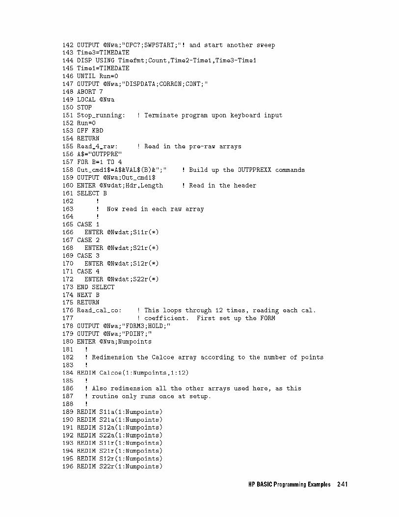
142 OUTPUT @Nwa;"OPC?;SWPSTART;"! and start another sweep
143 Time3=TIMEDATE
144 DISP USING Timefmt;Count,Time2-Time1,Time3-Time1
145 Time1=TIMEDATE
146 UNTIL Run=0
147 OUTPUT @Nwa;"DISPDATA;CORRON;CONT;"
148 ABORT 7
149 LOCAL @Nwa
150 STOP
151 Stop_running: ! Terminate program upon keyboard input
152 Run=0
153 OFF KBD
154 RETURN
155 Read_4_raw: ! Read in the pre-raw arrays
156 A$="OUTPPRE"
157 FOR B=1 TO 4
158 Out_cmd1$=A$&VAL$(B)&";" ! Build up the OUTPPREXX commands
159 OUTPUT @Nwa;Out_cmd1$
160 ENTER @Nwdat;Hdr,Length ! Read in the header
161 SELECT B
162 !
163 ! Now read in each raw array
164 !
165 CASE 1
166 ENTER @Nwdat;S11r(*)
167 CASE 2
168 ENTER @Nwdat;S21r(*)
169 CASE 3
170 ENTER @Nwdat;S12r(*)
171 CASE 4
172 ENTER @Nwdat;S22r(*)
173 END SELECT
174 NEXT B
175 RETURN
176 Read_cal_co: ! This loops through 12 times, reading each cal.
177 ! coefficient. First set up the FORM
178 OUTPUT @Nwa;"FORM3;HOLD;"
179 OUTPUT @Nwa;"POIN?;"
180 ENTER @Nwa;Numpoints
181 !
182 ! Redimension the Calcoe array according to the number of points
183 !
184 REDIM Calcoe(1:Numpoints,1:12)
185 !
186 ! Also redimension all the other arrays used here, as this
187 ! routine only runs once at setup.
188 !
189 REDIM S11a(1:Numpoints)
190 REDIM S21a(1:Numpoints)
191 REDIM S12a(1:Numpoints)
192 REDIM S22a(1:Numpoints)
193 REDIM S11r(1:Numpoints)
194 REDIM S21r(1:Numpoints)
195 REDIM S12r(1:Numpoints)
196 REDIM S22r(1:Numpoints)
HP BASIC Programming Examples 2-41
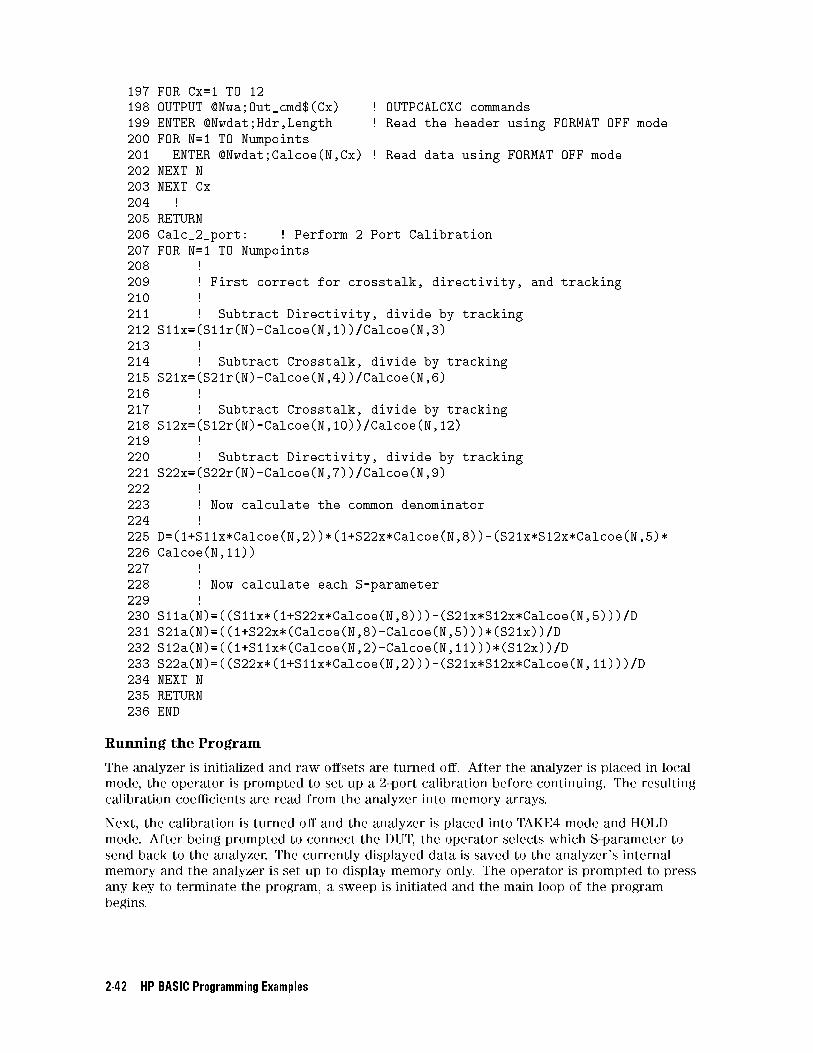
197 FOR Cx=1 TO 12
198 OUTPUT @Nwa;Out_cmd$(Cx) ! OUTPCALCXC commands
199 ENTER @Nwdat;Hdr,Length ! Read the header using FORMAT OFF mode
200 FOR N=1 TO Numpoints
201 ENTER @Nwdat;Calcoe(N,Cx) ! Read data using FORMAT OFF mode
202 NEXT N
203 NEXT Cx
204 !
205 RETURN
206 Calc_2_port: ! Perform 2 Port Calibration
207 FOR N=1 TO Numpoints
208 !
209 ! First correct for crosstalk, directivity, and tracking
210 !
211 ! Subtract Directivity, divide by tracking
212 S11x=(S11r(N)-Calcoe(N,1))/Calcoe(N,3)
213 !
214 ! Subtract Crosstalk, divide by tracking
215 S21x=(S21r(N)-Calcoe(N,4))/Calcoe(N,6)
216 !
217 ! Subtract Crosstalk, divide by tracking
218 S12x=(S12r(N)-Calcoe(N,10))/Calcoe(N,12)
219 !
220 ! Subtract Directivity, divide by tracking
221 S22x=(S22r(N)-Calcoe(N,7))/Calcoe(N,9)
222 !
223 ! Now calculate the common denominator
224 !
225 D=(1+S11x*Calcoe(N,2))*(1+S22x*Calcoe(N,8))-(S21x*S12x*Calcoe(N,5)*
226 Calcoe(N,11))
227 !
228 ! Now calculate each S-parameter
229 !
230 S11a(N)=((S11x*(1+S22x*Calcoe(N,8)))-(S21x*S12x*Calcoe(N,5)))/D
231 S21a(N)=((1+S22x*(Calcoe(N,8)-Calcoe(N,5)))*(S21x))/D
232 S12a(N)=((1+S11x*(Calcoe(N,2)-Calcoe(N,11)))*(S12x))/D
233 S22a(N)=((S22x*(1+S11x*Calcoe(N,2)))-(S21x*S12x*Calcoe(N,11)))/D
234 NEXT N
235 RETURN
236 END
Running the Program
The analyzer is initialized and raw o�sets are turned o�. After the analyzer is placed in local
mode, the operator is prompted to set up a 2-port calibration before continuing. The resulting
calibration coe�cients are read from the analyzer into memory arrays.
Next, the calibration is turned o� and the analyzer is placed into TAKE4 mode and HOLD
mode. After being prompted to connect the DUT, the operator selects which S-parameter to
send back to the analyzer. The currently displayed data is saved to the analyzer's internal
memory and the analyzer is set up to display memory only. The operator is prompted to press
any key to terminate the program, a sweep is initiated and the main loop of the program
begins.
2-42 HP BASIC Programming Examples

After the sweep concludes, the four pre-raw S-parameters are read from the analyzer into
memory arrays. The error-corrected (calibrated) S-parameters are calculated and the calibrated
data for the S-parameter selected earlier is read into the analyzer and saved to the analyzer's
internal memory. A new sweep is initiated and the loop repeats if there has been no keyboard
activity.
Upon exit of the loop, the analyzer is set up to display the active measurement trace. The
analyzer's internal calibration is turned back on and continuous sweep mode is resumed before
the program ends.
HP BASIC Programming Examples 2-43
Example 3: Measurement Data Transfer
There are two methods that can be used to read trace information from the analyzer:
selectively, using the trace markers
completely, using the trace-data array
If only speci�c information (such as a single point on the trace or the result of a marker
search) is required, the marker output command can be used to read the information. If all of
the trace data is required, see Examples 3B through 3E for examples of the various formats
available.
Trace-Data Formats and Transfers
Refer to Table 2-4. This table shows the number of bytes required to transfer a 201-point trace
in the di�erent formats. As you will see in the �rst example (FORM 4), ASCII data is the easiest
to transfer, but the most time consuming due to the number of bytes in the trace. If you are
using a PC-based controller, a more suitable format would be FORM 5. To use any trace data
format other than FORM 4 (ASCII data) requires some care in transferring the data to the
computer. Data types must be matched to read the bytes from the analyzer directly in to the
variable array. The computer must be told to stop formatting the incoming data and treat it
as a binary-data transfer. All of the other data formats also have a four byte header to deal
with. The �rst two bytes are the ASCII characters "#A" that indicate that a �xed length block
transfer follows, and the next two bytes form an integer containing the number of bytes in the
block to follow. The header must be read in to separate it from the rest of the block data that
is to be mapped into an array. \Array-Data Formats," located earlier in this chapter, discusses
the di�erent types of formats and their compositions.
Data may also be transferred from several di�erent locations in the trace-processing chain.
These examples will illustrate formatted-data transfers, but other locations in the trace-data
processing chains may be accessed. See Figure 1-3.
In this section, an example of each of the data formats will be shown for comparison. In
general, FORM 1 (internal binary format) should be used for traces that are not being utilized
for data content. Calibration data that is being transferred to a �le and back is good example.
See Example 3D.
Arrays which will be interpreted or processed within your program should be in FORM 2, 3 or
5, whichever is appropriate for your computer. Example 3C shows how to transfer a trace in
these formats.
In Examples 3B and 3C, the frequency counterpart of each data point in the array is also
determined. Many applications generate a frequency and magnitude, or a phase array for
the test results. Such data may be required for other data processing applications (such as
comparing data from other measurements).
In Example 3B, the frequency data is constructed from the frequency span information.
Alternatively, it is possible to read the frequencies directly out of the instrument with the
OUTPLIML command. OUTPLIML reports the limit-test results by transmitting the stimulus
point tested, a number indicating the limit-test results, and then the upper and lower limits at
that stimulus point (if available). The number indicating the limit results is a �1 for no test, 0
for fail, and 1 for pass. If there are no limits available, the analyzer transmits zeros. For this
example, we delete the limit test information and keep the stimulus information.
In Example 3C, the limit-test array is read into the controller and used to provide the values
directly from the analyzer memory. Reading from the limit-test array is convenient, although
it outputs the results in ASCII format (form 4), which may be slow. If there is no other way
to obtain the frequency data, this transfer time may be acceptable. Frequency information
becomes more di�cult to determine when not using the linear sweep mode. Log-frequency
2-44 HP BASIC Programming Examples
sweeps and list-frequency sweeps have quite di�erent values for each data point. For these
special cases, the additional time spent reading out the limit test results is an acceptable
solution for obtaining the valid frequency information for each data point in the trace.
Example 3A: Data Transfer Using Markers
Note This program is stored as EXAMP3A on the \Programming Examples" disk
received with the network analyzer.
Markers are the simplest form of trace-data transfer. A marker may be positioned using one of
three methods:
by a frequency location
by an actual data point location
by a trace-data value
In the following example, the marker is positioned on the trace's maximum value. Once
positioned on the trace, the trace data at that point can be read into the controller. The marker
data is always returned in FORM 4, ASCII format. Each number is sent as a 24-character
string. Characters can be digits, signs, or decimal points. All characters should be separated by
commas. In the case of markers, three numbers are sent. The display format determines the
values of the marker responses. See Table 1-4, \Units as a Function of Display Format."
When using trace data, it is important to control the network analyzer's sweep function (and
therefore the trace data) from the computer. Using the computer to control the instrument's
sweep insures that the data you read into the controller is in a quiescent or steady state. It also
insures that the measurement is complete.
The following is an outline of the program's processing sequence:
An I/O path is assigned for the analyzer.
The system is initialized.
The selected frequency span is swept once.
The marker is activated and placed on the maximum trace value.
The three marker values are output to the controller and displayed.
The instrument is returned to local control and the program ends.
HP BASIC Programming Examples 2-45
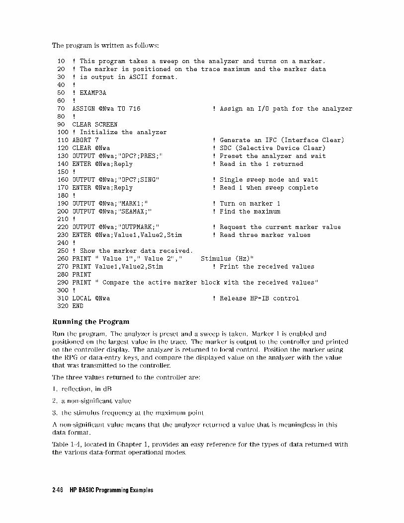
The program is written as follows:
10 ! This program takes a sweep on the analyzer and turns on a marker.
20 ! The marker is positioned on the trace maximum and the marker data
30 ! is output in ASCII format.
40 !
50 ! EXAMP3A
60 !
70 ASSIGN @Nwa TO 716 ! Assign an I/O path for the analyzer
80 !
90 CLEAR SCREEN
100 ! Initialize the analyzer
110 ABORT 7 ! Generate an IFC (Interface Clear)
120 CLEAR @Nwa ! SDC (Selective Device Clear)
130 OUTPUT @Nwa;"OPC?;PRES;" ! Preset the analyzer and wait
140 ENTER @Nwa;Reply ! Read in the 1 returned
150 !
160 OUTPUT @Nwa;"OPC?;SING" ! Single sweep mode and wait
170 ENTER @Nwa;Reply ! Read 1 when sweep complete
180 !
190 OUTPUT @Nwa;"MARK1;" ! Turn on marker 1
200 OUTPUT @Nwa;"SEAMAX;" ! Find the maximum
210 !
220 OUTPUT @Nwa;"OUTPMARK;" ! Request the current marker value
230 ENTER @Nwa;Value1,Value2,Stim ! Read three marker values
240 !
250 ! Show the marker data received.
260 PRINT " Value 1"," Value 2"," Stimulus (Hz)"
270 PRINT Value1,Value2,Stim ! Print the received values
280 PRINT
290 PRINT " Compare the active marker block with the received values"
300 !
310 LOCAL @Nwa ! Release HP-IB control
320 END
Running the Program
Run the program. The analyzer is preset and a sweep is taken. Marker 1 is enabled and
positioned on the largest value in the trace. The marker is output to the controller and printed
on the controller display. The analyzer is returned to local control. Position the marker using
the RPG or data-entry keys, and compare the displayed value on the analyzer with the value
that was transmitted to the controller.
The three values returned to the controller are:
1. re ection, in dB
2. a non-signi�cant value
3. the stimulus frequency at the maximum point
A non-signi�cant value means that the analyzer returned a value that is meaningless in this
data format.
Table 1-4, located in Chapter 1, provides an easy reference for the types of data returned with
the various data-format operational modes.
2-46 HP BASIC Programming Examples
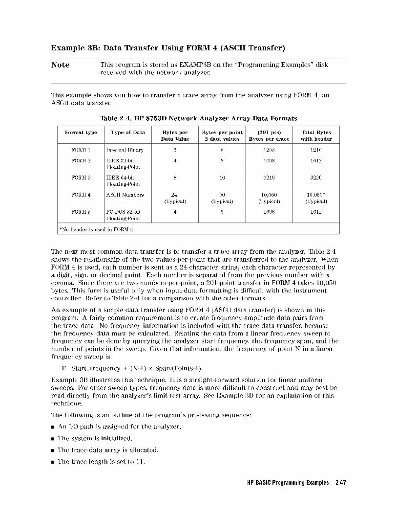
Example 3B: Data Transfer Using FORM 4 (ASCII Transfer)
Note This program is stored as EXAMP3B on the \Programming Examples" disk
received with the network analyzer.
This example shows you how to transfer a trace array from the analyzer using FORM 4, an
ASCII data transfer.
Table 2-4. HP 8753D Network Analyzer Array-Data Formats
Format type Type of Data Bytes per
Data Value
Bytes per point
2 data values
(201 pts)
Bytes per trace
Total Bytes
with header
FORM 1 Internal Binary 3 6 1206 1210
FORM 2 IEEE 32-bit
Floating-Point
4 8 1608 1612
FORM 3 IEEE 64-bit
Floating-Point
8 16 3216 3220
FORM 4 ASCII Numbers 24
(Typical)
50
(Typical)
10,050
(Typical)
10,050*
(Typical)
FORM 5 PC-DOS 32-bit
Floating-Point
4 8 1608 1612
*No header is used in FORM 4.
The next most common data transfer is to transfer a trace array from the analyzer. Table 2-4
shows the relationship of the two values-per-point that are transferred to the analyzer. When
FORM 4 is used, each number is sent as a 24-character string, each character represented by
a digit, sign, or decimal point. Each number is separated from the previous number with a
comma. Since there are two numbers-per-point, a 201-point transfer in FORM 4 takes 10,050
bytes. This form is useful only when input-data formatting is di�cult with the instrument
controller. Refer to Table 2-4 for a comparison with the other formats.
An example of a simple data transfer using FORM 4 (ASCII data transfer) is shown in this
program. A fairly common requirement is to create frequency-amplitude data pairs from
the trace data. No frequency information is included with the trace data transfer, because
the frequency data must be calculated. Relating the data from a linear frequency sweep to
frequency can be done by querying the analyzer start frequency, the frequency span, and the
number of points in the sweep. Given that information, the frequency of point N in a linear
frequency sweep is:
F=Start frequency + (N-1) � Span/(Points-1)
Example 3B illustrates this technique. It is a straight-forward solution for linear uniform
sweeps. For other sweep types, frequency data is more di�cult to construct and may best be
read directly from the analyzer's limit-test array. See Example 3D for an explanation of this
technique.
The following is an outline of the program's processing sequence:
An I/O path is assigned for the analyzer.
The system is initialized.
The trace-data array is allocated.
The trace length is set to 11.
HP BASIC Programming Examples 2-47
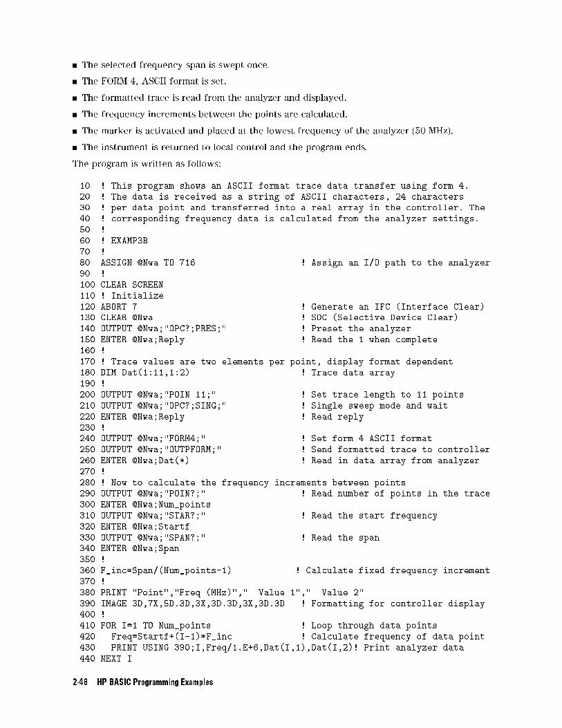
The selected frequency span is swept once.
The FORM 4, ASCII format is set.
The formatted trace is read from the analyzer and displayed.
The frequency increments between the points are calculated.
The marker is activated and placed at the lowest frequency of the analyzer (50 MHz).
The instrument is returned to local control and the program ends.
The program is written as follows:
10 ! This program shows an ASCII format trace data transfer using form 4.
20 ! The data is received as a string of ASCII characters, 24 characters
30 ! per data point and transferred into a real array in the controller. The
40 ! corresponding frequency data is calculated from the analyzer settings.
50 !
60 ! EXAMP3B
70 !
80 ASSIGN @Nwa TO 716 ! Assign an I/O path to the analyzer
90 !
100 CLEAR SCREEN
110 ! Initialize
120 ABORT 7 ! Generate an IFC (Interface Clear)
130 CLEAR @Nwa ! SDC (Selective Device Clear)
140 OUTPUT @Nwa;"OPC?;PRES;" ! Preset the analyzer
150 ENTER @Nwa;Reply ! Read the 1 when complete
160 !
170 ! Trace values are two elements per point, display format dependent
180 DIM Dat(1:11,1:2) ! Trace data array
190 !
200 OUTPUT @Nwa;"POIN 11;" ! Set trace length to 11 points
210 OUTPUT @Nwa;"OPC?;SING;" ! Single sweep mode and wait
220 ENTER @Nwa;Reply ! Read reply
230 !
240 OUTPUT @Nwa;"FORM4;" ! Set form 4 ASCII format
250 OUTPUT @Nwa;"OUTPFORM;" ! Send formatted trace to controller
260 ENTER @Nwa;Dat(*) ! Read in data array from analyzer
270 !
280 ! Now to calculate the frequency increments between points
290 OUTPUT @Nwa;"POIN?;" ! Read number of points in the trace
300 ENTER @Nwa;Num_points
310 OUTPUT @Nwa;"STAR?;" ! Read the start frequency
320 ENTER @Nwa;Startf
330 OUTPUT @Nwa;"SPAN?;" ! Read the span
340 ENTER @Nwa;Span
350 !
360 F_inc=Span/(Num_points-1) ! Calculate fixed frequency increment
370 !
380 PRINT "Point","Freq (MHz)"," Value 1"," Value 2"
390 IMAGE 3D,7X,5D.3D,3X,3D.3D,3X,3D.3D ! Formatting for controller display
400 !
410 FOR I=1 TO Num_points ! Loop through data points
420 Freq=Startf+(I-1)*F_inc ! Calculate frequency of data point
430 PRINT USING 390;I,Freq/1.E+6,Dat(I,1),Dat(I,2)! Print analyzer data
440 NEXT I
2-48 HP BASIC Programming Examples
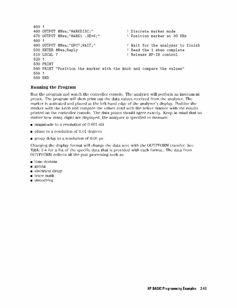
450 !
460 OUTPUT @Nwa;"MARKDISC;" ! Discrete marker mode
470 OUTPUT @Nwa;"MARK1 .3E+6;" ! Position marker at 30 KHz
480 !
490 OUTPUT @Nwa;"OPC?;WAIT;" ! Wait for the analyzer to finish
500 ENTER @Nwa;Reply ! Read the 1 when complete
510 LOCAL 7 ! Release HP-IB control
520 !
530 PRINT
540 PRINT "Position the marker with the knob and compare the values"
550 !
560 END
Running the Program
Run the program and watch the controller console. The analyzer will perform an instrument
preset. The program will then print out the data values received from the analyzer. The
marker is activated and placed at the left-hand edge of the analyzer's display. Position the
marker with the knob and compare the values read with the active marker with the results
printed on the controller console. The data points should agree exactly. Keep in mind that no
matter how many digits are displayed, the analyzer is speci�ed to measure:
magnitude to a resolution of 0.001 dB
phase to a resolution of 0.01 degrees
group delay to a resolution of 0.01 ps
Changing the display format will change the data sent with the OUTPFORM transfer. See
Table 2-4 for a list of the speci�c data that is provided with each format. The data from
OUTPFORM re ects all the post processing such as:
time domain
gating
electrical delay
trace math
smoothing
HP BASIC Programming Examples 2-49
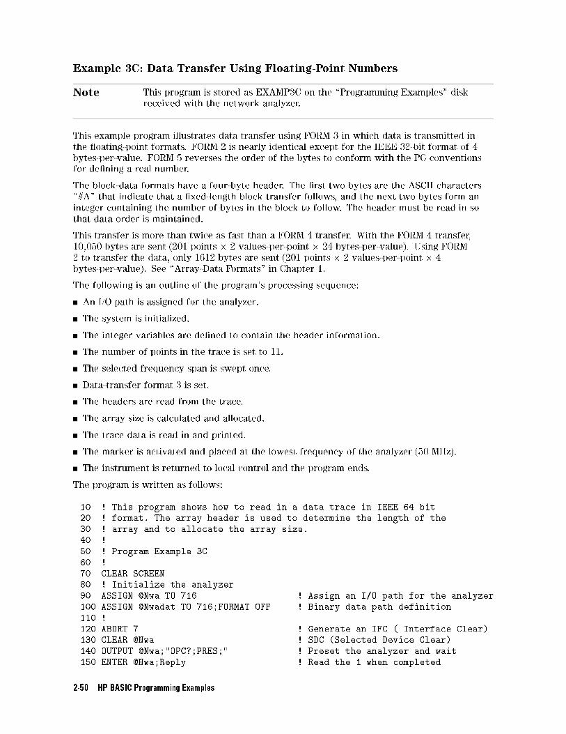
Example 3C: Data Transfer Using Floating-Point Numbers
Note This program is stored as EXAMP3C on the \Programming Examples" disk
received with the network analyzer.
This example program illustrates data transfer using FORM 3 in which data is transmitted in
the oating-point formats. FORM 2 is nearly identical except for the IEEE 32-bit format of 4
bytes-per-value. FORM 5 reverses the order of the bytes to conform with the PC conventions
for de�ning a real number.
The block-data formats have a four-byte header. The �rst two bytes are the ASCII characters
\#A" that indicate that a �xed-length block transfer follows, and the next two bytes form an
integer containing the number of bytes in the block to follow. The header must be read in so
that data order is maintained.
This transfer is more than twice as fast than a FORM 4 transfer. With the FORM 4 transfer,
10,050 bytes are sent (201 points � 2 values-per-point � 24 bytes-per-value). Using FORM
2 to transfer the data, only 1612 bytes are sent (201 points � 2 values-per-point � 4
bytes-per-value). See \Array-Data Formats" in Chapter 1.
The following is an outline of the program's processing sequence:
An I/O path is assigned for the analyzer.
The system is initialized.
The integer variables are de�ned to contain the header information.
The number of points in the trace is set to 11.
The selected frequency span is swept once.
Data-transfer format 3 is set.
The headers are read from the trace.
The array size is calculated and allocated.
The trace data is read in and printed.
The marker is activated and placed at the lowest frequency of the analyzer (50 MHz).
The instrument is returned to local control and the program ends.
The program is written as follows:
10 ! This program shows how to read in a data trace in IEEE 64 bit
20 ! format. The array header is used to determine the length of the
30 ! array and to allocate the array size.
40 !
50 ! Program Example 3C
60 !
70 CLEAR SCREEN
80 ! Initialize the analyzer
90 ASSIGN @Nwa TO 716 ! Assign an I/O path for the analyzer
100 ASSIGN @Nwadat TO 716;FORMAT OFF ! Binary data path definition
110 !
120 ABORT 7 ! Generate an IFC ( Interface Clear)
130 CLEAR @Nwa ! SDC (Selected Device Clear)
140 OUTPUT @Nwa;"OPC?;PRES;" ! Preset the analyzer and wait
150 ENTER @Nwa;Reply ! Read the 1 when completed
2-50 HP BASIC Programming Examples
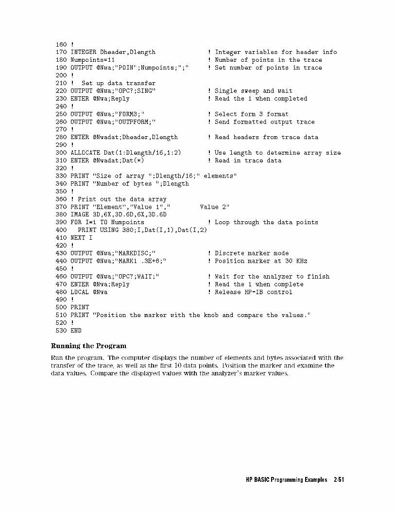
160 !
170 INTEGER Dheader,Dlength ! Integer variables for header info
180 Numpoints=11 ! Number of points in the trace
190 OUTPUT @Nwa;"POIN";Numpoints;";" ! Set number of points in trace
200 !
210 ! Set up data transfer
220 OUTPUT @Nwa;"OPC?;SING" ! Single sweep and wait
230 ENTER @Nwa;Reply ! Read the 1 when completed
240 !
250 OUTPUT @Nwa;"FORM3;" ! Select form 3 format
260 OUTPUT @Nwa;"OUTPFORM;" ! Send formatted output trace
270 !
280 ENTER @Nwadat;Dheader,Dlength ! Read headers from trace data
290 !
300 ALLOCATE Dat(1:Dlength/16,1:2) ! Use length to determine array size
310 ENTER @Nwadat;Dat(*) ! Read in trace data
320 !
330 PRINT "Size of array ";Dlength/16;" elements"
340 PRINT "Number of bytes ";Dlength
350 !
360 ! Print out the data array
370 PRINT "Element","Value 1"," Value 2"
380 IMAGE 3D,6X,3D.6D,6X,3D.6D
390 FOR I=1 TO Numpoints ! Loop through the data points
400 PRINT USING 380;I,Dat(I,1),Dat(I,2)
410 NEXT I
420 !
430 OUTPUT @Nwa;"MARKDISC;" ! Discrete marker mode
440 OUTPUT @Nwa;"MARK1 .3E+6;" ! Position marker at 30 KHz
450 !
460 OUTPUT @Nwa;"OPC?;WAIT;" ! Wait for the analyzer to finish
470 ENTER @Nwa;Reply ! Read the 1 when complete
480 LOCAL @Nwa ! Release HP-IB control
490 !
500 PRINT
510 PRINT "Position the marker with the knob and compare the values."
520 !
530 END
Running the Program
Run the program. The computer displays the number of elements and bytes associated with the
transfer of the trace, as well as the �rst 10 data points. Position the marker and examine the
data values. Compare the displayed values with the analyzer's marker values.
HP BASIC Programming Examples 2-51
Example 3D: Data Transfer Using Frequency-Array Information
Note This program is stored as EXAMP3D on the \Programming Examples" disk
received with the network analyzer.
Example 3C was used to read in the trace-data array. Example 3D explains how to use the
limit-test array to read the corresponding frequency values for the completed trace array
into the controller. The analyzer is set to sweep from 50 MHz to 200 MHz in log-frequency
mode with the number of points in the trace set to 11. This makes it very di�cult to compute
the frequency-point spacing in the trace. The points are equally spaced across the trace, but
not equally spaced in relation to frequency (because the frequency span is displayed in a
logarithmic scale, as opposed to a linear scale). The limit-test data array may be read from
the analyzer to provide the frequency values for each data point. Four values are read for
each data point on the analyzer. The test results and limit values are not used in this example.
Only the frequency values are used. This technique is an e�ective method of obtaining the
non-linear frequency data from the analyzer display. The test data and frequencies are printed
on the controller display and the marker is enabled to allow the operator to examine the actual
locations on the analyzer display.
The following is an outline of the program's processing sequence:
An I/O path is assigned for the analyzer.
The system is initialized.
The integer variables for the header information are de�ned.
The number of points in the trace is set to 11.
The frequency span (50 MHz to 200 MHz) is selected.
The log-frequency sweep is selected.
The data-transfer format 3 is set.
The headers are read from the trace.
The array size is calculated and allocated.
The trace data is read in.
The limit-test array is calculated and allocated.
The limit-line test array is read in.
The table header is printed.
The program cycles through the trace values.
The trace data and frequency are printed.
The discrete-marker mode is activated.
The marker is activated and placed at the lowest frequency of the analyzer (50 MHz).
The instrument is returned to local control and the program ends.
2-52 HP BASIC Programming Examples
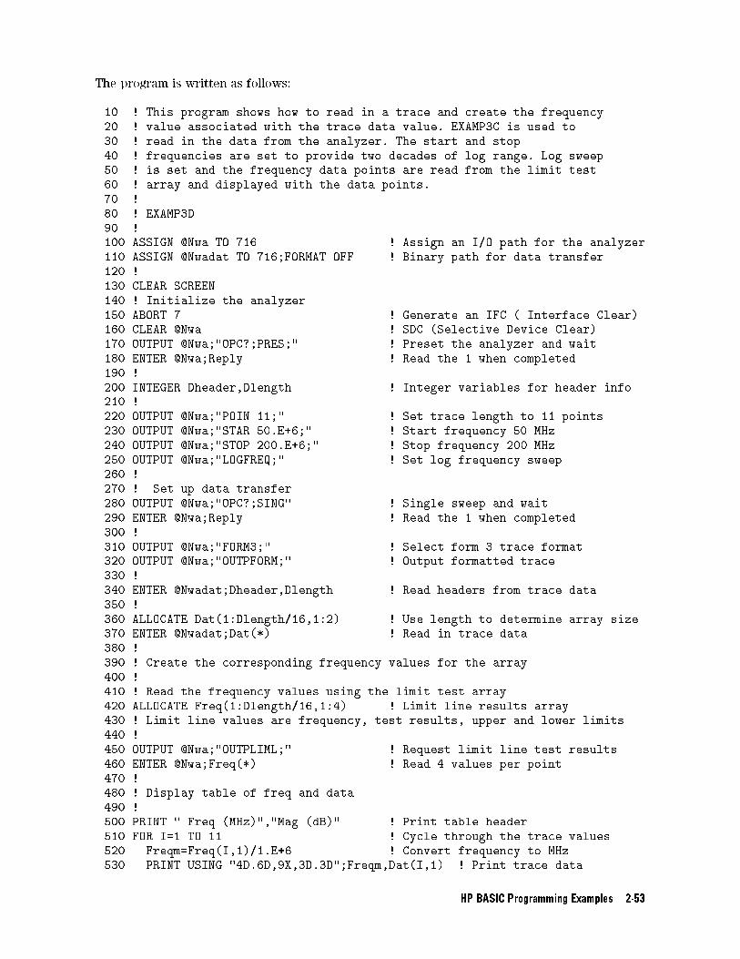
The program is written as follows:
10 ! This program shows how to read in a trace and create the frequency
20 ! value associated with the trace data value. EXAMP3C is used to
30 ! read in the data from the analyzer. The start and stop
40 ! frequencies are set to provide two decades of log range. Log sweep
50 ! is set and the frequency data points are read from the limit test
60 ! array and displayed with the data points.
70 !
80 ! EXAMP3D
90 !
100 ASSIGN @Nwa TO 716 ! Assign an I/O path for the analyzer
110 ASSIGN @Nwadat TO 716;FORMAT OFF ! Binary path for data transfer
120 !
130 CLEAR SCREEN
140 ! Initialize the analyzer
150 ABORT 7 ! Generate an IFC ( Interface Clear)
160 CLEAR @Nwa ! SDC (Selective Device Clear)
170 OUTPUT @Nwa;"OPC?;PRES;" ! Preset the analyzer and wait
180 ENTER @Nwa;Reply ! Read the 1 when completed
190 !
200 INTEGER Dheader,Dlength ! Integer variables for header info
210 !
220 OUTPUT @Nwa;"POIN 11;" ! Set trace length to 11 points
230 OUTPUT @Nwa;"STAR 50.E+6;" ! Start frequency 50 MHz
240 OUTPUT @Nwa;"STOP 200.E+6;" ! Stop frequency 200 MHz
250 OUTPUT @Nwa;"LOGFREQ;" ! Set log frequency sweep
260 !
270 ! Set up data transfer
280 OUTPUT @Nwa;"OPC?;SING" ! Single sweep and wait
290 ENTER @Nwa;Reply ! Read the 1 when completed
300 !
310 OUTPUT @Nwa;"FORM3;" ! Select form 3 trace format
320 OUTPUT @Nwa;"OUTPFORM;" ! Output formatted trace
330 !
340 ENTER @Nwadat;Dheader,Dlength ! Read headers from trace data
350 !
360 ALLOCATE Dat(1:Dlength/16,1:2) ! Use length to determine array size
370 ENTER @Nwadat;Dat(*) ! Read in trace data
380 !
390 ! Create the corresponding frequency values for the array
400 !
410 ! Read the frequency values using the limit test array
420 ALLOCATE Freq(1:Dlength/16,1:4) ! Limit line results array
430 ! Limit line values are frequency, test results, upper and lower limits
440 !
450 OUTPUT @Nwa;"OUTPLIML;" ! Request limit line test results
460 ENTER @Nwa;Freq(*) ! Read 4 values per point
470 !
480 ! Display table of freq and data
490 !
500 PRINT " Freq (MHz)","Mag (dB)" ! Print table header
510 FOR I=1 TO 11 ! Cycle through the trace values
520 Freqm=Freq(I,1)/1.E+6 ! Convert frequency to MHz
530 PRINT USING "4D.6D,9X,3D.3D";Freqm,Dat(I,1) ! Print trace data
HP BASIC Programming Examples 2-53
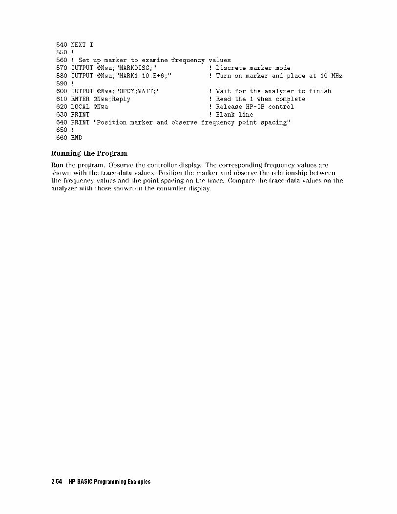
540 NEXT I
550 !
560 ! Set up marker to examine frequency values
570 OUTPUT @Nwa;"MARKDISC;" ! Discrete marker mode
580 OUTPUT @Nwa;"MARK1 10.E+6;" ! Turn on marker and place at 10 MHz
590 !
600 OUTPUT @Nwa;"OPC?;WAIT;" ! Wait for the analyzer to finish
610 ENTER @Nwa;Reply ! Read the 1 when complete
620 LOCAL @Nwa ! Release HP-IB control
630 PRINT ! Blank line
640 PRINT "Position marker and observe frequency point spacing"
650 !
660 END
Running the Program
Run the program. Observe the controller display. The corresponding frequency values are
shown with the trace-data values. Position the marker and observe the relationship between
the frequency values and the point spacing on the trace. Compare the trace-data values on the
analyzer with those shown on the controller display.
2-54 HP BASIC Programming Examples
Example 3E: Data Transfer Using FORM 1 (Internal-Binary Format)
Note This program is stored as EXAMP3E on the \Programming Examples" disk
received with the network analyzer.
FORM 1 is used for rapid I/O transfer of analyzer data. It contains the least number of
bytes-per-trace and does not require re-formatting in the analyzer. This format is more di�cult
to convert into a numeric array in the controller.
The following is an outline of the program's processing sequence:
An I/O path is assigned for the analyzer.
The system is initialized.
The integer variables for the header information are de�ned.
The string variable for the header is de�ned.
The selected frequency span is swept once.
The internal-binary format is selected.
The error-corrected data is output from the analyzer.
The two data-header characters and the two length bytes are read in.
The string bu�er is allocated for data.
The trace data is read into the string bu�er.
The analyzer is restored to continuous-sweep mode and queried for command completion.
The instrument is returned to local control and the program ends.
HP BASIC Programming Examples 2-55
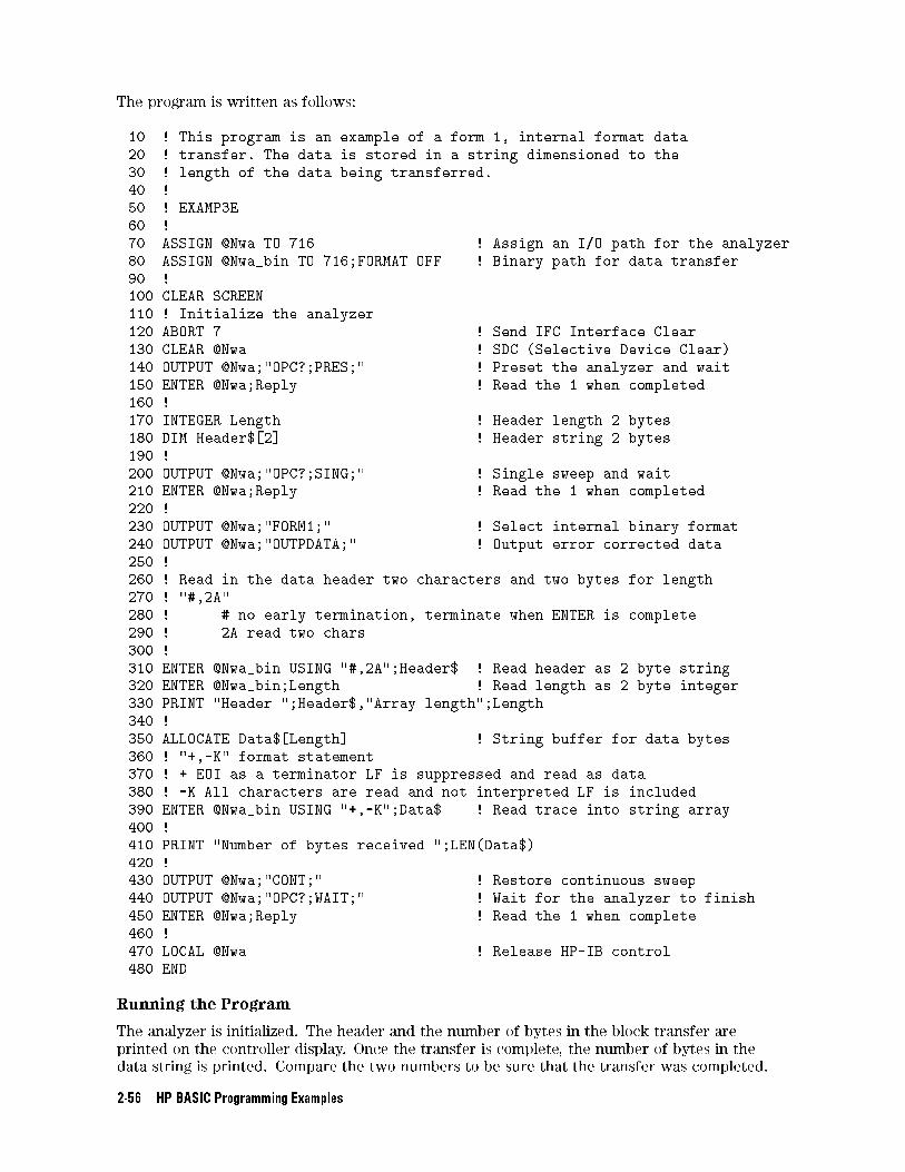
The program is written as follows:
10 ! This program is an example of a form 1, internal format data
20 ! transfer. The data is stored in a string dimensioned to the
30 ! length of the data being transferred.
40 !
50 ! EXAMP3E
60 !
70 ASSIGN @Nwa TO 716 ! Assign an I/O path for the analyzer
80 ASSIGN @Nwa_bin TO 716;FORMAT OFF ! Binary path for data transfer
90 !
100 CLEAR SCREEN
110 ! Initialize the analyzer
120 ABORT 7 ! Send IFC Interface Clear
130 CLEAR @Nwa ! SDC (Selective Device Clear)
140 OUTPUT @Nwa;"OPC?;PRES;" ! Preset the analyzer and wait
150 ENTER @Nwa;Reply ! Read the 1 when completed
160 !
170 INTEGER Length ! Header length 2 bytes
180 DIM Header$[2] ! Header string 2 bytes
190 !
200 OUTPUT @Nwa;"OPC?;SING;" ! Single sweep and wait
210 ENTER @Nwa;Reply ! Read the 1 when completed
220 !
230 OUTPUT @Nwa;"FORM1;" ! Select internal binary format
240 OUTPUT @Nwa;"OUTPDATA;" ! Output error corrected data
250 !
260 ! Read in the data header two characters and two bytes for length
270 ! "#,2A"
280 ! # no early termination, terminate when ENTER is complete
290 ! 2A read two chars
300 !
310 ENTER @Nwa_bin USING "#,2A";Header$ ! Read header as 2 byte string
320 ENTER @Nwa_bin;Length ! Read length as 2 byte integer
330 PRINT "Header ";Header$,"Array length";Length
340 !
350 ALLOCATE Data$[Length] ! String buffer for data bytes
360 ! "+,-K" format statement
370 ! + EOI as a terminator LF is suppressed and read as data
380 ! -K All characters are read and not interpreted LF is included
390 ENTER @Nwa_bin USING "+,-K";Data$ ! Read trace into string array
400 !
410 PRINT "Number of bytes received ";LEN(Data$)
420 !
430 OUTPUT @Nwa;"CONT;" ! Restore continuous sweep
440 OUTPUT @Nwa;"OPC?;WAIT;" ! Wait for the analyzer to finish
450 ENTER @Nwa;Reply ! Read the 1 when complete
460 !
470 LOCAL @Nwa ! Release HP-IB control
480 END
Running the Program
The analyzer is initialized. The header and the number of bytes in the block transfer are
printed on the controller display. Once the transfer is complete, the number of bytes in the
data string is printed. Compare the two numbers to be sure that the transfer was completed.
2-56 HP BASIC Programming Examples
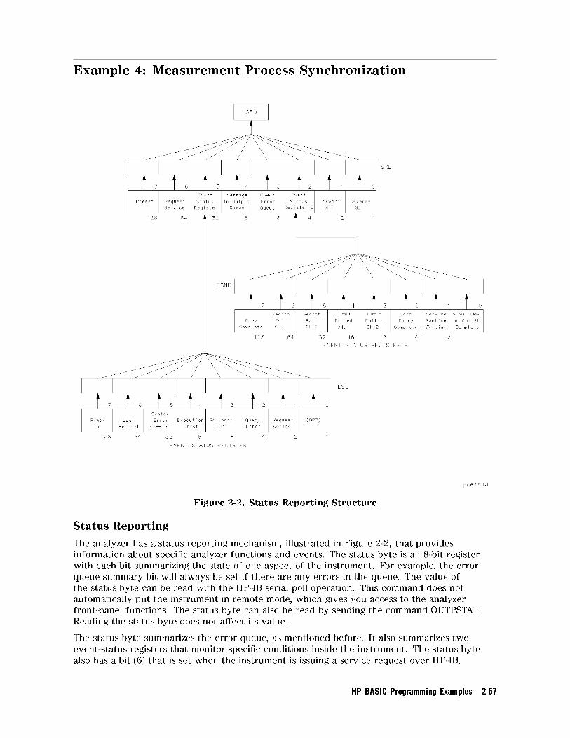
Example 4: Measurement Process Synchronization
Figure 2-2. Status Reporting Structure
Status Reporting
The analyzer has a status reporting mechanism, illustrated in Figure 2-2, that provides
information about speci�c analyzer functions and events. The status byte is an 8-bit register
with each bit summarizing the state of one aspect of the instrument. For example, the error
queue summary bit will always be set if there are any errors in the queue. The value of
the status byte can be read with the HP-IB serial poll operation. This command does not
automatically put the instrument in remote mode, which gives you access to the analyzer
front-panel functions. The status byte can also be read by sending the command OUTPSTAT.
Reading the status byte does not a�ect its value.
The status byte summarizes the error queue, as mentioned before. It also summarizes two
event-status registers that monitor speci�c conditions inside the instrument. The status byte
also has a bit (6) that is set when the instrument is issuing a service request over HP-IB,
HP BASIC Programming Examples 2-57
and a bit (0) that is set in the event-status register when the analyzer has data to send out
over HP-IB. See \Error Reporting," located in Chapter 1, for a discussion of the event-status
registers.
Example 4A: Using the Error Queue
Note This program is stored as EXAMP4A on the \Programming Examples" disk
received with the network analyzer.
The error queue holds up to 20 instrument errors and warnings in the order that they occurred.
Each time the analyzer detects an error condition, the analyzer displays a message, and puts
the error in the error queue. If there are any errors in the queue, bit 3 of the status byte will
be set. The errors can be read from the queue with the OUTPERRO command. OUTPERRO
causes the analyzer to transmit the error number and message of the oldest error in the queue.
The following is an outline of the program's processing sequence:
An I/O path is assigned for the analyzer.
The system is initialized.
The error-message string is allocated.
The analyzer is released from remote control.
The program begins an endless loop to read the error queue.
The status byte is read with a serial poll.
The program tests to see if an error is present in the queue.
The error-queue bit is set.
The program requests the content of the error queue.
The error number and string are read.
The error messages are printed until there are no more errors in the queue.
The instrument is returned to local control.
The controller emits a beep to attach the attention of the operator and resumes searching for
errors.
2-58 HP BASIC Programming Examples
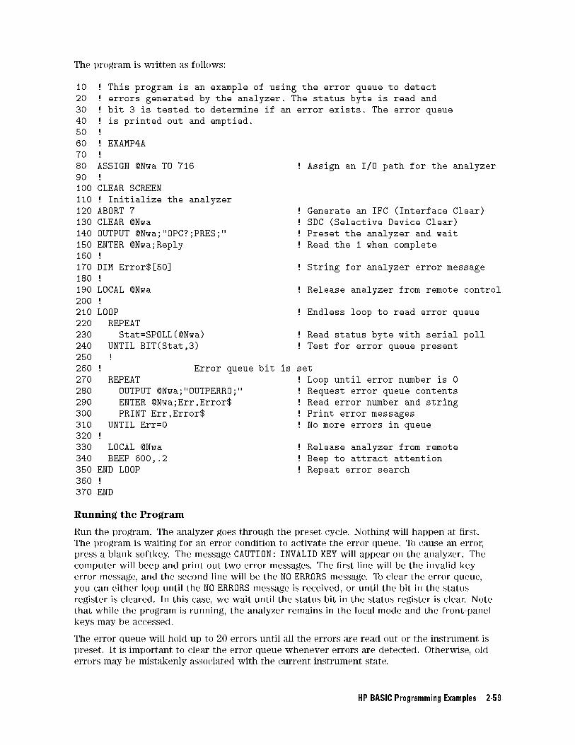
The program is written as follows:
10 ! This program is an example of using the error queue to detect
20 ! errors generated by the analyzer. The status byte is read and
30 ! bit 3 is tested to determine if an error exists. The error queue
40 ! is printed out and emptied.
50 !
60 ! EXAMP4A
70 !
80 ASSIGN @Nwa TO 716 ! Assign an I/O path for the analyzer
90 !
100 CLEAR SCREEN
110 ! Initialize the analyzer
120 ABORT 7 ! Generate an IFC (Interface Clear)
130 CLEAR @Nwa ! SDC (Selective Device Clear)
140 OUTPUT @Nwa;"OPC?;PRES;" ! Preset the analyzer and wait
150 ENTER @Nwa;Reply ! Read the 1 when complete
160 !
170 DIM Error$[50] ! String for analyzer error message
180 !
190 LOCAL @Nwa ! Release analyzer from remote control
200 !
210 LOOP ! Endless loop to read error queue
220 REPEAT
230 Stat=SPOLL(@Nwa) ! Read status byte with serial poll
240 UNTIL BIT(Stat,3) ! Test for error queue present
250 !
260 ! Error queue bit is set
270 REPEAT ! Loop until error number is 0
280 OUTPUT @Nwa;"OUTPERRO;" ! Request error queue contents
290 ENTER @Nwa;Err,Error$ ! Read error number and string
300 PRINT Err,Error$ ! Print error messages
310 UNTIL Err=0 ! No more errors in queue
320 !
330 LOCAL @Nwa ! Release analyzer from remote
340 BEEP 600,.2 ! Beep to attract attention
350 END LOOP ! Repeat error search
360 !
370 END
Running the Program
Run the program. The analyzer goes through the preset cycle. Nothing will happen at �rst.
The program is waiting for an error condition to activate the error queue. To cause an error,
press a blank softkey. The message CAUTION: INVALID KEY will appear on the analyzer. The
computer will beep and print out two error messages. The �rst line will be the invalid key
error message, and the second line will be the NO ERRORS message. To clear the error queue,
you can either loop until the NO ERRORS message is received, or until the bit in the status
register is cleared. In this case, we wait until the status bit in the status register is clear. Note
that while the program is running, the analyzer remains in the local mode and the front-panel
keys may be accessed.
The error queue will hold up to 20 errors until all the errors are read out or the instrument is
preset. It is important to clear the error queue whenever errors are detected. Otherwise, old
errors may be mistakenly associated with the current instrument state.
HP BASIC Programming Examples 2-59
Press �System� and then the unlabeled key several times quickly and watch the display. The
number of errors observed should correspond to the number of times you pressed the key.
As another example, press �Cal�NNNNNNNNNNNNNNNNNNNNNNNNNNNNNNNNNNNNNNNNNCORRECTION ON . A complete list of error messages and their
descriptions can be found in \Error Messages" of the HP 8753D Network Analyzer User's
Guide.
The program is in an in�nite loop waiting for errors to occur. End the program by pressing
�RESET� or �BREAK� on the controller keyboard.
Note Not all messages displayed by the analyzer are put in the error queue: operator
prompts and cautions are not included.
2-60 HP BASIC Programming Examples
Example 4B: Generating Interrupts
Note This program is stored as EXAMP4B on the \Programming Examples" disk
received with the network analyzer.
It is also possible to generate interrupts using the status-reporting mechanism. The status-byte
bits can be enabled to generate a service request (SRQ) when set. In turn, the instrument
controller can be set up to generate an interrupt on the SRQ and respond to the condition
which caused the SRQ.
To generate an SRQ, a bit in the status byte is enabled using the command SREn. A one (1)
in a bit position enables that bit in the status byte. Hence, SRE 8 enables an SRQ on bit 3,
the check-error queue, since the decimal value 8 equals 00001000 in binary representation.
Whenever an error is put into the error queue and bit 3 is set, the SRQ line is asserted,
illuminating the (S) indicator in the HP-IB status block on the front panel of the analyzer. The
only way to clear the SRQ is to disable bit 3, re-enable bit 3, or read out all the errors from the
queue.
A bit in the event-status register can be enabled so that it is summarized by bit 5 of the status
byte. If any enabled bit in the event-status register is set, bit 5 of the status byte will also
be set. For example ESE 66 enables bits 1 and 6 of the event-status register, since in binary,
the decimal number 66 equals 01000010. Hence, whenever active control is requested or a
front-panel key is pressed, bit 5 of the status byte will be set. Similarly, ESNBn enables bits in
event-status register B so that they will be summarized by bit 2 in the status byte.
To generate an SRQ from an event-status register, enable the desired event-status register
bit. Then enable the status byte to generate an SRQ. For instance, ESE 32;SRE 32; enables
the syntax-error bit. When the syntax-error bit is set, the summary bit in the status byte will
be set. This will, in turn, enable an SRQ on bit 5 of the status byte, the summary bit for the
event-status register.
The following is an outline of the program's processing sequence:
An I/O path is assigned for the analyzer.
The system is initialized.
The status registers are cleared.
The event-status register bit 5 is enabled.
The status-register bit 5 is enabled.
The interrupt pointer is enabled and points to a subroutine.
Two bad commands are set to the analyzer to generate errors.
The controller reads a serial-poll byte from HP-IB in the event of an interrupt.
The program tests for an SRQ.
If the SRQ is not generated by the analyzer, the subroutine stops and displays SRQ FROM
OTHER DEVICE.
If the SRQ was generated by the analyzer, the program reads the status byte and event-status
register.
If bit 5 in the event-status register is set, program prints: SYNTAX ERROR FROM ANALYZER.
If bit 5 in the event-status register is NOT set, program prints: SYNTAX ERROR BIT NOT SET.
The SRQ interrupt is re-enabled on the bus.
HP BASIC Programming Examples 2-61
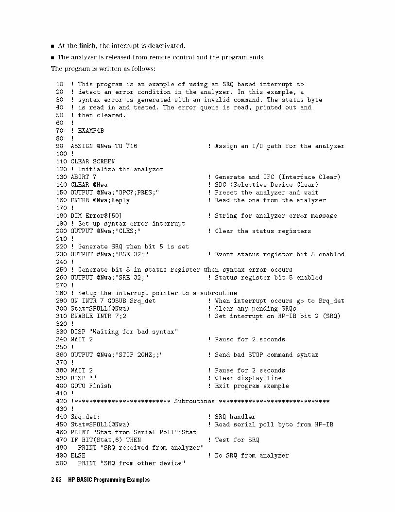
At the �nish, the interrupt is deactivated.
The analyzer is released from remote control and the program ends.
The program is written as follows:
10 ! This program is an example of using an SRQ based interrupt to
20 ! detect an error condition in the analyzer. In this example, a
30 ! syntax error is generated with an invalid command. The status byte
40 ! is read in and tested. The error queue is read, printed out and
50 ! then cleared.
60 !
70 ! EXAMP4B
80 !
90 ASSIGN @Nwa TO 716 ! Assign an I/O path for the analyzer
100 !
110 CLEAR SCREEN
120 ! Initialize the analyzer
130 ABORT 7 ! Generate and IFC (Interface Clear)
140 CLEAR @Nwa ! SDC (Selective Device Clear)
150 OUTPUT @Nwa;"OPC?;PRES;" ! Preset the analyzer and wait
160 ENTER @Nwa;Reply ! Read the one from the analyzer
170 !
180 DIM Error$[50] ! String for analyzer error message
190 ! Set up syntax error interrupt
200 OUTPUT @Nwa;"CLES;" ! Clear the status registers
210 !
220 ! Generate SRQ when bit 5 is set
230 OUTPUT @Nwa;"ESE 32;" ! Event status register bit 5 enabled
240 !
250 ! Generate bit 5 in status register when syntax error occurs
260 OUTPUT @Nwa;"SRE 32;" ! Status register bit 5 enabled
270 !
280 ! Setup the interrupt pointer to a subroutine
290 ON INTR 7 GOSUB Srq_det ! When interrupt occurs go to Srq_det
300 Stat=SPOLL(@Nwa) ! Clear any pending SRQs
310 ENABLE INTR 7;2 ! Set interrupt on HP-IB bit 2 (SRQ)
320 !
330 DISP "Waiting for bad syntax"
340 WAIT 2 ! Pause for 2 seconds
350 !
360 OUTPUT @Nwa;"STIP 2GHZ;;" ! Send bad STOP command syntax
370 !
380 WAIT 2 ! Pause for 2 seconds
390 DISP "" ! Clear display line
400 GOTO Finish ! Exit program example
410 !
420 !************************** Subroutines ******************************
430 !
440 Srq_det: ! SRQ handler
450 Stat=SPOLL(@Nwa) ! Read serial poll byte from HP-IB
460 PRINT "Stat from Serial Poll";Stat
470 IF BIT(Stat,6) THEN ! Test for SRQ
480 PRINT "SRQ received from analyzer"
490 ELSE ! No SRQ from analyzer
500 PRINT "SRQ from other device"
2-62 HP BASIC Programming Examples
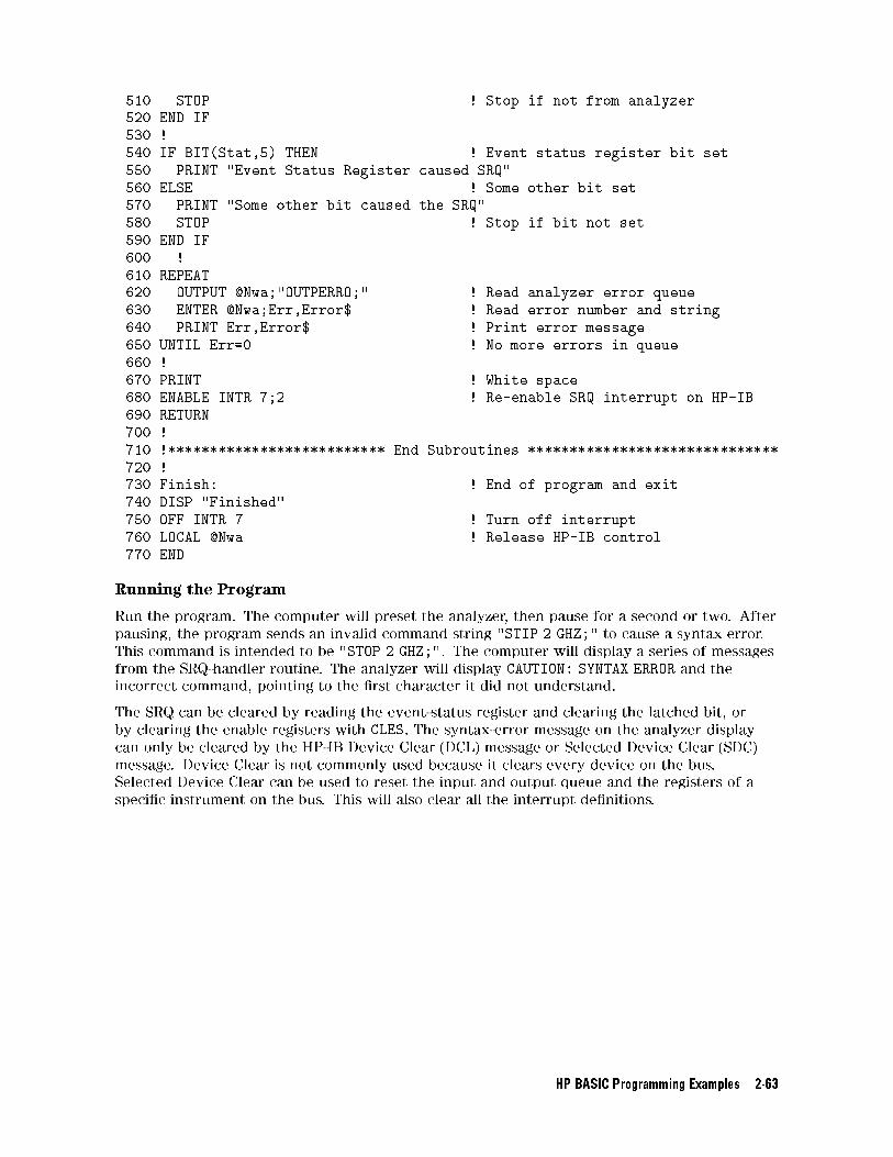
510 STOP ! Stop if not from analyzer
520 END IF
530 !
540 IF BIT(Stat,5) THEN ! Event status register bit set
550 PRINT "Event Status Register caused SRQ"
560 ELSE ! Some other bit set
570 PRINT "Some other bit caused the SRQ"
580 STOP ! Stop if bit not set
590 END IF
600 !
610 REPEAT
620 OUTPUT @Nwa;"OUTPERRO;" ! Read analyzer error queue
630 ENTER @Nwa;Err,Error$ ! Read error number and string
640 PRINT Err,Error$ ! Print error message
650 UNTIL Err=0 ! No more errors in queue
660 !
670 PRINT ! White space
680 ENABLE INTR 7;2 ! Re-enable SRQ interrupt on HP-IB
690 RETURN
700 !
710 !************************** End Subroutines ******************************
720 !
730 Finish: ! End of program and exit
740 DISP "Finished"
750 OFF INTR 7 ! Turn off interrupt
760 LOCAL @Nwa ! Release HP-IB control
770 END
Running the Program
Run the program. The computer will preset the analyzer, then pause for a second or two. After
pausing, the program sends an invalid command string "STIP 2 GHZ;" to cause a syntax error.
This command is intended to be "STOP 2 GHZ;". The computer will display a series of messages
from the SRQ-handler routine. The analyzer will display CAUTION: SYNTAX ERROR and the
incorrect command, pointing to the �rst character it did not understand.
The SRQ can be cleared by reading the event-status register and clearing the latched bit, or
by clearing the enable registers with CLES. The syntax-error message on the analyzer display
can only be cleared by the HP-IB Device Clear (DCL) message or Selected Device Clear (SDC)
message. Device Clear is not commonly used because it clears every device on the bus.
Selected Device Clear can be used to reset the input and output queue and the registers of a
speci�c instrument on the bus. This will also clear all the interrupt de�nitions.
HP BASIC Programming Examples 2-63
Example 4C: Power Meter Calibration
Note This program is stored as EXAMP4C on the \Programming Examples" disk
received with the network analyzer.
For increased accuracy of the analyzer's PORT 1-output power, a power meter calibration is
available. This measurement-accuracy enhancement technique is described in \Optimizing
Measurement Results" of the HP 8753D Network Analyzer User's Guide. The example
described will perform the sample and sweep calibration under HP-IB remote control.
The power meter is usually connected to PORT 1 for the forward measurements. Its address
must be set correctly and it must be connected to the HP-IB. The power meter address can be
set by pressing: �Local�NNNNNNNNNNNNNNNNNNNNNNNNNNNNNNNNNNNNNNNNNSET ADDRESSES
NNNNNNNNNNNNNNNNNNNNNNNNNNNNNNNNNNNNNNNNNNNNNNNNNNNNNNNNADDRESS P MTR/HPIB and using the �*� and �+� keys or
the numeric key pad to complete the process. The appropriate command must be selected for
the model number of power meter being used. PressNNNNNNNNNNNNNNNNNNNNNNNNNNNNNNNNNNNNNNNNNNNNPOWER MTR: [ ] until the model being
used is displayed between the brackets.
The correction factors for the power sensor are entered into the analyzer. All of these steps are
explained in the \Optimizing Measurement Results" chapter of the HP 8753D Network Analyzer
User's Guide.
The number of readings-per-point must also be selected before starting. The number of points
directly a�ects the measurement time of the calibration sequence. The power meter must
be triggered and read by the analyzer for each trace point. Typically, two readings-per-point
is considered appropriate. More than two readings-per-point could lead to unacceptable
processing time.
To control a power meter calibration via HP-IB, the analyzer must be set to pass-control mode.
The analyzer must step to the next point in the sweep and read the power present at the
power meter sensor. For this operation to take place, the system controller must set up the
measurement and then pass control to the analyzer to read each data point in the sweep. After
reading the data point from the power meter, the analyzer passes control back to the system
controller. The analyzer then sets up to measure the next point and again requests control from
the system controller. This process continues until the analyzer signals that the entire sweep
has been measured point-by-point.
The following is an outline of the program's processing sequence:
An I/O path is assigned for the analyzer.
The system is initialized.
The number of points in the trace is set.
The number of readings-per-point is set.
The frequency span is set.
Note The frequency span of this example program must be modi�ed in order to
correspond to the frequency ranges of the HP 8753D.
The reference channel is measured.
The power meter calibration array is allocated.
The power meter model is chosen.
The status registers are cleared.
2-64 HP BASIC Programming Examples
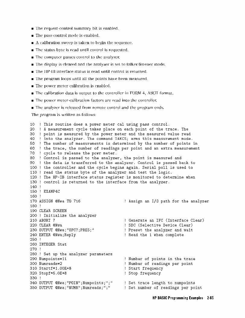
The request-control summary bit is enabled.
The pass-control mode is enabled.
A calibration sweep is taken to begin the sequence.
The status byte is read until control is requested.
The computer passes control to the analyzer.
The display is cleared and the analyzer is set to talker/listener mode.
The HP-IB interface status is read until control is returned.
The program loops until all the points have been measured.
The power meter calibration is enabled.
The calibration data is output to the controller in FORM 4, ASCII format.
The power meter-calibration factors are read into the controller.
The analyzer is released from remote control and the program ends.
The program is written as follows:
10 ! This routine does a power meter cal using pass control.
20 ! A measurement cycle takes place on each point of the trace. The
30 ! point is measured by the power meter and the measured value read
40 ! into the analyzer. The command TAKCS; arms this measurement mode.
50 ! The number of measurements is determined by the number of points in
60 ! the trace, the number of readings per point and an extra measurement
70 ! cycle to release the powr meter.
80 ! Control is passed to the analyzer, the point is measured and
90 ! the data is transferred to the analyzer. Control is passed back to
100 ! the controller and the cycle begins again. Serial poll is used to
110 ! read the status byte of the analyzer and test the logic.
120 ! The HP-IB interface status register is monitored to determine when
130 ! control is returned to the interface from the analyzer.
140 !
150 ! EXAMP4C
160 !
170 ASSIGN @Nwa TO 716 ! Assign an I/O path for the analyzer
180 !
190 CLEAR SCREEN
200 ! Initialize the analyzer
210 ABORT 7 ! Generate an IFC (Interface Clear)
220 CLEAR @Nwa ! SDC (Selective Device Clear)
230 OUTPUT @Nwa;"OPC?;PRES;" ! Preset the analyzer and wait
240 ENTER @Nwa;Reply ! Read the 1 when complete
250 !
260 INTEGER Stat
270 !
280 ! Set up the analyzer parameters
290 Numpoints=11 ! Number of points in the trace
300 Numreads=2 ! Number of readings per point
310 Startf=1.00E+8 ! Start frequency
320 Stopf=5.0E+8 ! Stop frequency
330 !
340 OUTPUT @Nwa;"POIN";Numpoints;";" ! Set trace length to numpoints
350 OUTPUT @Nwa;"NUMR";Numreads;";" ! Set number of readings per point
HP BASIC Programming Examples 2-65
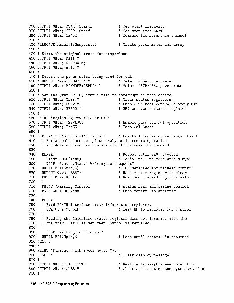
360 OUTPUT @Nwa;"STAR";Startf ! Set start frequency
370 OUTPUT @Nwa;"STOP";Stopf ! Set stop frequency
380 OUTPUT @Nwa;"MEASR;" ! Measure the reference channel
390 !
400 ALLOCATE Pmcal(1:Numpoints) ! Create power meter cal array
410 !
420 ! Store the original trace for comparison
430 OUTPUT @Nwa;"DATI;"
440 OUTPUT @Nwa;"DISPDATM;"
450 OUTPUT @Nwa;"AUTO;"
460 !
470 ! Select the power meter being used for cal
480 ! OUTPUT @Nwa;"POWM ON;" ! Select 436A power meter
490 OUTPUT @Nwa;"POWMOFF;DEBUON;" ! Select 437B/438A power meter
500 !
510 ! Set analyzer HP-IB, status regs to interrupt on pass control
520 OUTPUT @Nwa;"CLES;" ! Clear status registers
530 OUTPUT @Nwa;"ESE2;" ! Enable request control summary bit
540 OUTPUT @Nwa;"SRE32;" ! SRQ on events status register
550 !
560 PRINT "Beginning Power Meter CAL"
570 OUTPUT @Nwa;"USEPASC;" ! Enable pass control operation
580 OUTPUT @Nwa;"TAKCS;" ! Take Cal Sweep
590 !
600 FOR I=1 TO Numpoints*Numreads+1 ! Points * Number of readings plus 1
610 ! Serial poll does not place analyzer in remote operation
620 ! and does not require the analyzer to process the command.
630 !
640 REPEAT ! Repeat until SRQ detected
650 Stat=SPOLL(@Nwa) ! Serial poll to read status byte
660 DISP "Stat ";Stat;" Waiting for request"
670 UNTIL BIT(Stat,6) ! SRQ detected for request control
680 OUTPUT @Nwa;"ESR?;" ! Read status register to clear
690 ENTER @Nwa;Reply ! Read and discard register value
700 !
710 PRINT "Passing Control" ! status read and pasing control
720 PASS CONTROL @Nwa ! Pass control to analyzer
730 !
740 REPEAT
750 ! Read HP-IB interface state information register.
760 STATUS 7,6;Hpib ! Test HP-IB register for control
770 !
780 ! Reading the interface status register does not interact with the
790 ! analyzer. Bit 6 is set when control is returned.
800 !
810 DISP "Waiting for control"
820 UNTIL BIT(Hpib,6) ! Loop until control is returned
830 NEXT I
840 !
850 PRINT "Finished with Power meter Cal"
860 DISP "" ! Clear display message
870 !
880 OUTPUT @Nwa;"TALKLIST;" ! Restore Talker/Listener operation
890 OUTPUT @Nwa;"CLES;" ! Clear and reset status byte operation
900 !
2-66 HP BASIC Programming Examples
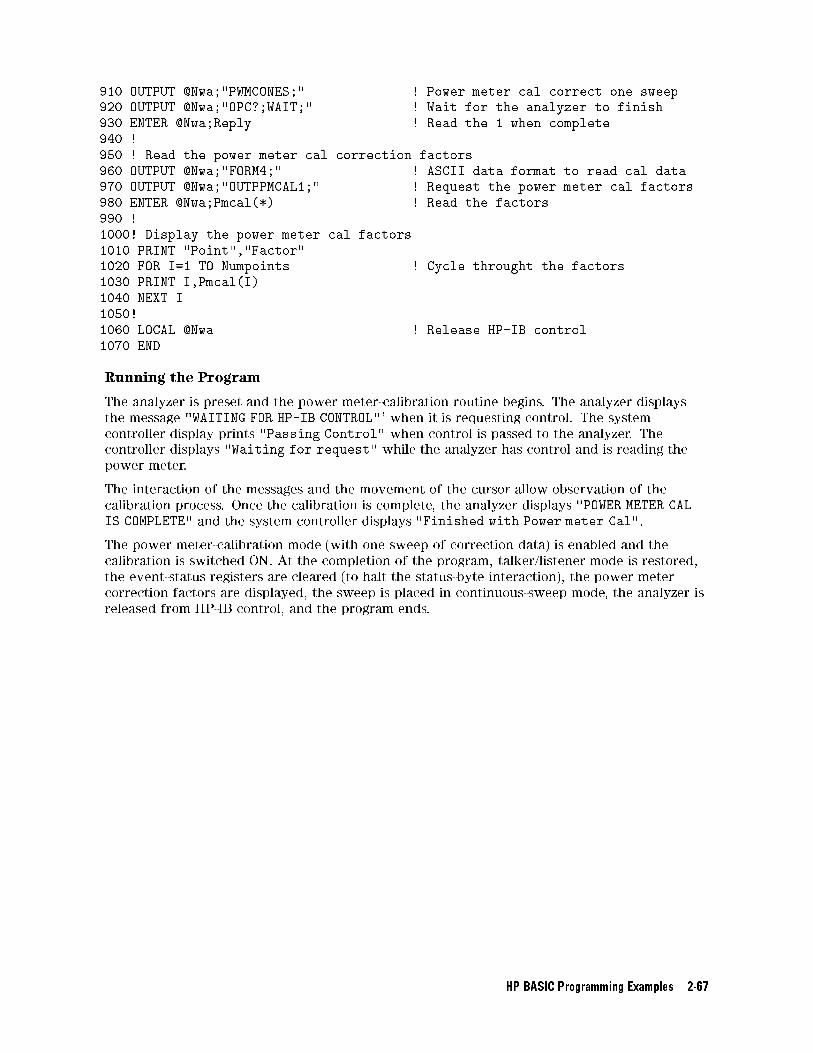
910 OUTPUT @Nwa;"PWMCONES;" ! Power meter cal correct one sweep
920 OUTPUT @Nwa;"OPC?;WAIT;" ! Wait for the analyzer to finish
930 ENTER @Nwa;Reply ! Read the 1 when complete
940 !
950 ! Read the power meter cal correction factors
960 OUTPUT @Nwa;"FORM4;" ! ASCII data format to read cal data
970 OUTPUT @Nwa;"OUTPPMCAL1;" ! Request the power meter cal factors
980 ENTER @Nwa;Pmcal(*) ! Read the factors
990 !
1000! Display the power meter cal factors
1010 PRINT "Point","Factor"
1020 FOR I=1 TO Numpoints ! Cycle throught the factors
1030 PRINT I,Pmcal(I)
1040 NEXT I
1050!
1060 LOCAL @Nwa ! Release HP-IB control
1070 END
Running the Program
The analyzer is preset and the power meter-calibration routine begins. The analyzer displays
the message "WAITING FOR HP-IB CONTROL"' when it is requesting control. The system
controller display prints "Passing Control" when control is passed to the analyzer. The
controller displays "Waiting for request" while the analyzer has control and is reading the
power meter.
The interaction of the messages and the movement of the cursor allow observation of the
calibration process. Once the calibration is complete, the analyzer displays "POWER METER CAL
IS COMPLETE" and the system controller displays "Finished with Power meter Cal".
The power meter-calibration mode (with one sweep of correction data) is enabled and the
calibration is switched ON. At the completion of the program, talker/listener mode is restored,
the event-status registers are cleared (to halt the status-byte interaction), the power meter
correction factors are displayed, the sweep is placed in continuous-sweep mode, the analyzer is
released from HP-IB control, and the program ends.
HP BASIC Programming Examples 2-67

Example 5: Network Analyzer System Setups
Saving and Recalling Instrument States
Note The most e�cient option for storing and recalling analyzer states is using the
analyzer's internal registers to save the CAL data. Recalling these registers is
the fastest solution to restoring analyzer setups. See \Printing, Plotting, or
Saving Measurement Results" in the HP 8753D Network Analyzer User's Guide
for detailed information on the analyzer's internal storage registers.
In the event that all the registers have been used, the internal disk drive is
not used, or if internal memory limitations exist, then these external solutions
become viable.
The purpose of this example is to demonstrate several programming options for storing and
recalling entire instrument states over HP-IB. The examples describe two di�erent processes for
storing and recalling instrument states. The �rst example accomplishes the task using the learn
string. The second example involves reading both the learn string and the calibration arrays
out of the analyzer and storing them to disk or storing them in the system controller itself.
Using the learn string is a very rapid way of saving the instrument state, but using direct disk
access has the advantage of automatically storing calibrations, cal kits, and data along with the
instrument state.
A complete analyzer setup requires sending the learn string and a calibration array to set
the analyzer parameters. The CAL array may also be placed in the analyzer, just as if a
calibration was performed. By sending both sets of data, the analyzer may be quickly setup for
a measurement.
Several di�erent measurements may be required in the course of testing a device. An e�cient
way of performing multiple measurements is to send both the calibration array and the learn
string, and then perform the measurements.
Example 5A: Using the Learn String
Note This program is stored as EXAMP5A on the \Programming Examples" disk
received with the network analyzer.
The learn string is a very fast and easy way to read an instrument state. The learn string
includes all front-panel settings, the limit table for each channel, and the list-frequency table.
It can be read out of the analyzer with the command OUTPLEAS, and input to the analyzer
with the command INPULEAS. The example for a FORM 1 transfer could also have been used.
However, Example 5A is the simplest solution for reading the learn string from the analyzer.
The following is an outline of the program's processing sequence:
An I/O path is assigned for the analyzer.
The system is initialized.
The string storage is allocated.
The learn string is requested.
The string is read without any processing.
The analyzer is released from remote control.
2-68 HP BASIC Programming Examples
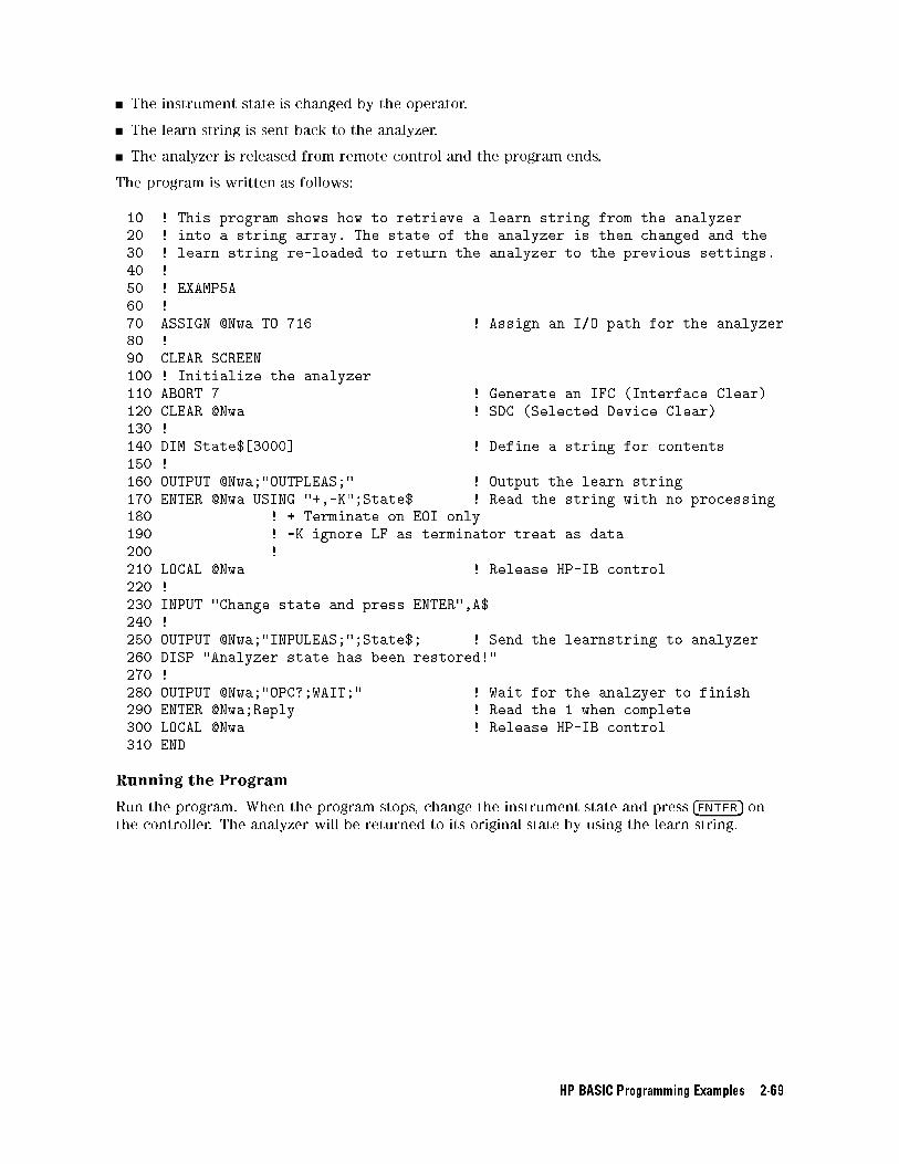
The instrument state is changed by the operator.
The learn string is sent back to the analyzer.
The analyzer is released from remote control and the program ends.
The program is written as follows:
10 ! This program shows how to retrieve a learn string from the analyzer
20 ! into a string array. The state of the analyzer is then changed and the
30 ! learn string re-loaded to return the analyzer to the previous settings.
40 !
50 ! EXAMP5A
60 !
70 ASSIGN @Nwa TO 716 ! Assign an I/O path for the analyzer
80 !
90 CLEAR SCREEN
100 ! Initialize the analyzer
110 ABORT 7 ! Generate an IFC (Interface Clear)
120 CLEAR @Nwa ! SDC (Selected Device Clear)
130 !
140 DIM State$[3000] ! Define a string for contents
150 !
160 OUTPUT @Nwa;"OUTPLEAS;" ! Output the learn string
170 ENTER @Nwa USING "+,-K";State$ ! Read the string with no processing
180 ! + Terminate on EOI only
190 ! -K ignore LF as terminator treat as data
200 !
210 LOCAL @Nwa ! Release HP-IB control
220 !
230 INPUT "Change state and press ENTER",A$
240 !
250 OUTPUT @Nwa;"INPULEAS;";State$; ! Send the learnstring to analyzer
260 DISP "Analyzer state has been restored!"
270 !
280 OUTPUT @Nwa;"OPC?;WAIT;" ! Wait for the analzyer to finish
290 ENTER @Nwa;Reply ! Read the 1 when complete
300 LOCAL @Nwa ! Release HP-IB control
310 END
Running the Program
Run the program. When the program stops, change the instrument state and press �ENTER� onthe controller. The analyzer will be returned to its original state by using the learn string.
HP BASIC Programming Examples 2-69
Example 5B: Reading Calibration Data
Note This program is stored as EXAMP5B on the \Programming Examples" disk
received with the network analyzer.
This example demonstrates:
how to read measurement calibration data out of the network analyzer
how to read it back into the analyzer
how to determine which calibration is active
The data used to perform measurement-error correction is stored inside the analyzer in one (or
more) of twelve calibration-coe�cient arrays. Each array is a speci�c error coe�cient, and is
stored and transmitted as an error-corrected data array. Each point is a real/imaginary pair,
and the number of points in the array is the same as the number of points in the sweep. The
�ve data formats also apply to the transfer of calibration-coe�cient arrays. \Printing, Plotting,
or Saving Measurement Results" in the HP 8753D Network Analyzer User's Guide contains
information on the storage locations for calibration coe�cients and di�erent calibration types.
A computer can read out the error coe�cients using the commands OUTPCALC01,
OUTPCALC02, . . . through OUTPCALC12. Each calibration type uses only as many arrays as
required, beginning with array 1. Hence, it is necessary to know the type of calibration about
to be read out: attempting to read an array not being used in the current calibration causes the
"REQUESTED DATA NOT CURRENTLY AVAILABLE" warning.
A computer can also store calibration coe�cients in the analyzer. To do this, declare the type
of calibration data about to be stored in the analyzer just as if you were about to perform that
calibration. Then, instead of calling up di�erent classes, transfer the calibration coe�cients
using the INPUCALCnn; commands. The variables nn are a data pair appended to the command
representing a calibration number from 01 through 12. When all the coe�cients are stored in
the analyzer, activate the calibration by issuing the mnemonic SAVC;, and trigger a sweep on
the analyzer.
This example reads the calibration coe�cients into a very large array, from which they can be
examined, modi�ed, stored, or put back into the instrument. If the data is to be directly stored
on to disk, it is usually more e�cient to use FORM 1 (analyzer's internal-binary format), and to
store each coe�cient array as it is read in.
The following is an outline of the program's processing sequence:
An I/O path is assigned for the analyzer.
A binary path is assigned.
The system is initialized.
The calibration types and number of arrays are de�ned.
The integer variables for reading the headers are de�ned.
The calibration type and number of arrays are read by the controller.
The output is formatted in FORM 3.
The number of points in the trace is read.
The memory is allocated for the calibration arrays.
Each calibration array is requested from the analyzer.
Header information is read with a binary I/O path.
2-70 HP BASIC Programming Examples
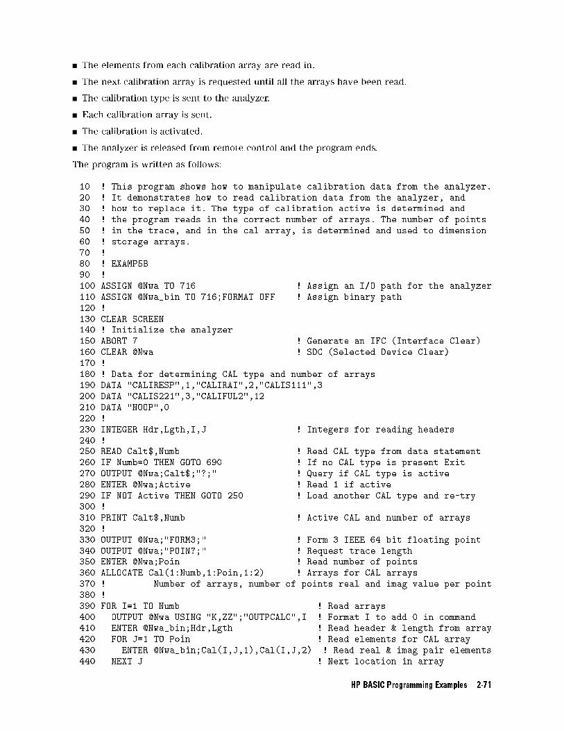
The elements from each calibration array are read in.
The next calibration array is requested until all the arrays have been read.
The calibration type is sent to the analyzer.
Each calibration array is sent.
The calibration is activated.
The analyzer is released from remote control and the program ends.
The program is written as follows:
10 ! This program shows how to manipulate calibration data from the analyzer.
20 ! It demonstrates how to read calibration data from the analyzer, and
30 ! how to replace it. The type of calibration active is determined and
40 ! the program reads in the correct number of arrays. The number of points
50 ! in the trace, and in the cal array, is determined and used to dimension
60 ! storage arrays.
70 !
80 ! EXAMP5B
90 !
100 ASSIGN @Nwa TO 716 ! Assign an I/O path for the analyzer
110 ASSIGN @Nwa_bin TO 716;FORMAT OFF ! Assign binary path
120 !
130 CLEAR SCREEN
140 ! Initialize the analyzer
150 ABORT 7 ! Generate an IFC (Interface Clear)
160 CLEAR @Nwa ! SDC (Selected Device Clear)
170 !
180 ! Data for determining CAL type and number of arrays
190 DATA "CALIRESP",1,"CALIRAI",2,"CALIS111",3
200 DATA "CALIS221",3,"CALIFUL2",12
210 DATA "NOOP",0
220 !
230 INTEGER Hdr,Lgth,I,J ! Integers for reading headers
240 !
250 READ Calt$,Numb ! Read CAL type from data statement
260 IF Numb=0 THEN GOTO 690 ! If no CAL type is present Exit
270 OUTPUT @Nwa;Calt$;"?;" ! Query if CAL type is active
280 ENTER @Nwa;Active ! Read 1 if active
290 IF NOT Active THEN GOTO 250 ! Load another CAL type and re-try
300 !
310 PRINT Calt$,Numb ! Active CAL and number of arrays
320 !
330 OUTPUT @Nwa;"FORM3;" ! Form 3 IEEE 64 bit floating point
340 OUTPUT @Nwa;"POIN?;" ! Request trace length
350 ENTER @Nwa;Poin ! Read number of points
360 ALLOCATE Cal(1:Numb,1:Poin,1:2) ! Arrays for CAL arrays
370 ! Number of arrays, number of points real and imag value per point
380 !
390 FOR I=1 TO Numb ! Read arrays
400 OUTPUT @Nwa USING "K,ZZ";"OUTPCALC",I ! Format I to add 0 in command
410 ENTER @Nwa_bin;Hdr,Lgth ! Read header & length from array
420 FOR J=1 TO Poin ! Read elements for CAL array
430 ENTER @Nwa_bin;Cal(I,J,1),Cal(I,J,2) ! Read real & imag pair elements
440 NEXT J ! Next location in array
HP BASIC Programming Examples 2-71
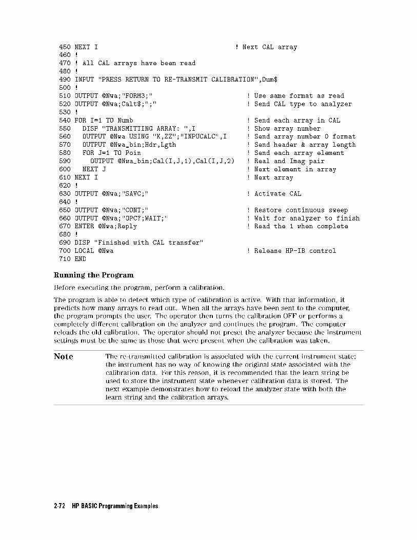
450 NEXT I ! Next CAL array
460 !
470 ! All CAL arrays have been read
480 !
490 INPUT "PRESS RETURN TO RE-TRANSMIT CALIBRATION",Dum$
500 !
510 OUTPUT @Nwa;"FORM3;" ! Use same format as read
520 OUTPUT @Nwa;Calt$;";" ! Send CAL type to analyzer
530 !
540 FOR I=1 TO Numb ! Send each array in CAL
550 DISP "TRANSMITTING ARRAY: ",I ! Show array number
560 OUTPUT @Nwa USING "K,ZZ";"INPUCALC",I ! Send array number 0 format
570 OUTPUT @Nwa_bin;Hdr,Lgth ! Send header & array length
580 FOR J=1 TO Poin ! Send each array element
590 OUTPUT @Nwa_bin;Cal(I,J,1),Cal(I,J,2) ! Real and Imag pair
600 NEXT J ! Next element in array
610 NEXT I ! Next array
620 !
630 OUTPUT @Nwa;"SAVC;" ! Activate CAL
640 !
650 OUTPUT @Nwa;"CONT;" ! Restore continuous sweep
660 OUTPUT @Nwa;"OPC?;WAIT;" ! Wait for analyzer to finish
670 ENTER @Nwa;Reply ! Read the 1 when complete
680 !
690 DISP "Finished with CAL transfer"
700 LOCAL @Nwa ! Release HP-IB control
710 END
Running the Program
Before executing the program, perform a calibration.
The program is able to detect which type of calibration is active. With that information, it
predicts how many arrays to read out. When all the arrays have been sent to the computer,
the program prompts the user. The operator then turns the calibration OFF or performs a
completely di�erent calibration on the analyzer and continues the program. The computer
reloads the old calibration. The operator should not preset the analyzer because the instrument
settings must be the same as those that were present when the calibration was taken.
Note The re-transmitted calibration is associated with the current instrument state:
the instrument has no way of knowing the original state associated with the
calibration data. For this reason, it is recommended that the learn string be
used to store the instrument state whenever calibration data is stored. The
next example demonstrates how to reload the analyzer state with both the
learn string and the calibration arrays.
2-72 HP BASIC Programming Examples
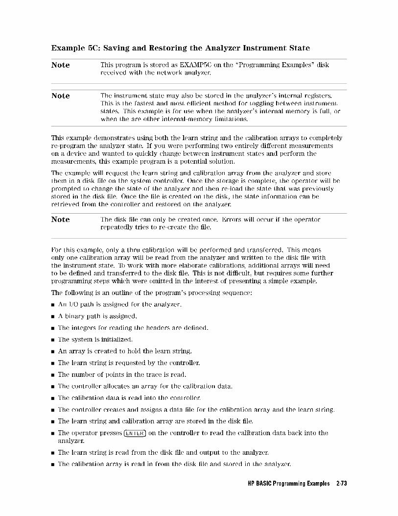
Example 5C: Saving and Restoring the Analyzer Instrument State
Note This program is stored as EXAMP5C on the \Programming Examples" disk
received with the network analyzer.
Note The instrument state may also be stored in the analyzer's internal registers.
This is the fastest and most e�cient method for toggling between instrument
states. This example is for use when the analyzer's internal memory is full, or
when the are other internal-memory limitations.
This example demonstrates using both the learn string and the calibration arrays to completely
re-program the analyzer state. If you were performing two entirely di�erent measurements
on a device and wanted to quickly change between instrument states and perform the
measurements, this example program is a potential solution.
The example will request the learn string and calibration array from the analyzer and store
them in a disk �le on the system controller. Once the storage is complete, the operator will be
prompted to change the state of the analyzer and then re-load the state that was previously
stored in the disk �le. Once the �le is created on the disk, the state information can be
retrieved from the controller and restored on the analyzer.
Note The disk �le can only be created once. Errors will occur if the operator
repeatedly tries to re-create the �le.
For this example, only a thru calibration will be performed and transferred. This means
only one calibration array will be read from the analyzer and written to the disk �le with
the instrument state. To work with more elaborate calibrations, additional arrays will need
to be de�ned and transferred to the disk �le. This is not di�cult, but requires some further
programming steps which were omitted in the interest of presenting a simple example.
The following is an outline of the program's processing sequence:
An I/O path is assigned for the analyzer.
A binary path is assigned.
The integers for reading the headers are de�ned.
The system is initialized.
An array is created to hold the learn string.
The learn string is requested by the controller.
The number of points in the trace is read.
The controller allocates an array for the calibration data.
The calibration data is read into the controller.
The controller creates and assigns a data �le for the calibration array and the learn string.
The learn string and calibration array are stored in the disk �le.
The operator presses �ENTER� on the controller to read the calibration data back into the
analyzer.
The learn string is read from the disk �le and output to the analyzer.
The calibration array is read in from the disk �le and stored in the analyzer.
HP BASIC Programming Examples 2-73
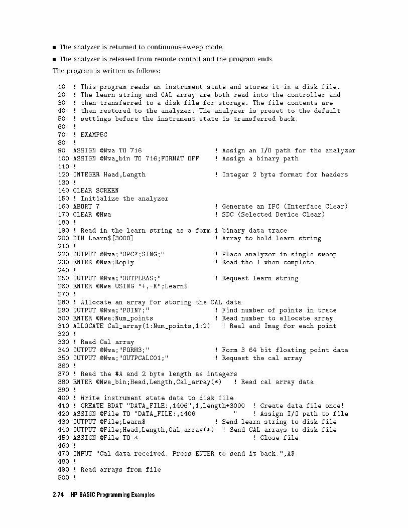
The analyzer is returned to continuous-sweep mode.
The analyzer is released from remote control and the program ends.
The program is written as follows:
10 ! This program reads an instrument state and stores it in a disk file.
20 ! The learn string and CAL array are both read into the controller and
30 ! then transferred to a disk file for storage. The file contents are
40 ! then restored to the analyzer. The analyzer is preset to the default
50 ! settings before the instrument state is transferred back.
60 !
70 ! EXAMP5C
80 !
90 ASSIGN @Nwa TO 716 ! Assign an I/O path for the analyzer
100 ASSIGN @Nwa_bin TO 716;FORMAT OFF ! Assign a binary path
110 !
120 INTEGER Head,Length ! Integer 2 byte format for headers
130 !
140 CLEAR SCREEN
150 ! Initialize the analyzer
160 ABORT 7 ! Generate an IFC (Interface Clear)
170 CLEAR @Nwa ! SDC (Selected Device Clear)
180 !
190 ! Read in the learn string as a form 1 binary data trace
200 DIM Learn$[3000] ! Array to hold learn string
210 !
220 OUTPUT @Nwa;"OPC?;SING;" ! Place analyzer in single sweep
230 ENTER @Nwa;Reply ! Read the 1 when complete
240 !
250 OUTPUT @Nwa;"OUTPLEAS;" ! Request learn string
260 ENTER @Nwa USING "+,-K";Learn$
270 !
280 ! Allocate an array for storing the CAL data
290 OUTPUT @Nwa;"POIN?;" ! Find number of points in trace
300 ENTER @Nwa;Num_points ! Read number to allocate array
310 ALLOCATE Cal_array(1:Num_points,1:2) ! Real and Imag for each point
320 !
330 ! Read Cal array
340 OUTPUT @Nwa;"FORM3;" ! Form 3 64 bit floating point data
350 OUTPUT @Nwa;"OUTPCALC01;" ! Request the cal array
360 !
370 ! Read the #A and 2 byte length as integers
380 ENTER @Nwa_bin;Head,Length,Cal_array(*) ! Read cal array data
390 !
400 ! Write instrument state data to disk file
410 ! CREATE BDAT "DATA_FILE:,1406",1,Length+3000 ! Create data file once!
420 ASSIGN @File TO "DATA_FILE:,1406 " ! Assign I/O path to file
430 OUTPUT @File;Learn$ ! Send learn string to disk file
440 OUTPUT @File;Head,Length,Cal_array(*) ! Send CAL arrays to disk file
450 ASSIGN @File TO * ! Close file
460 !
470 INPUT "Cal data received. Press ENTER to send it back.",A$
480 !
490 ! Read arrays from file
500 !
2-74 HP BASIC Programming Examples
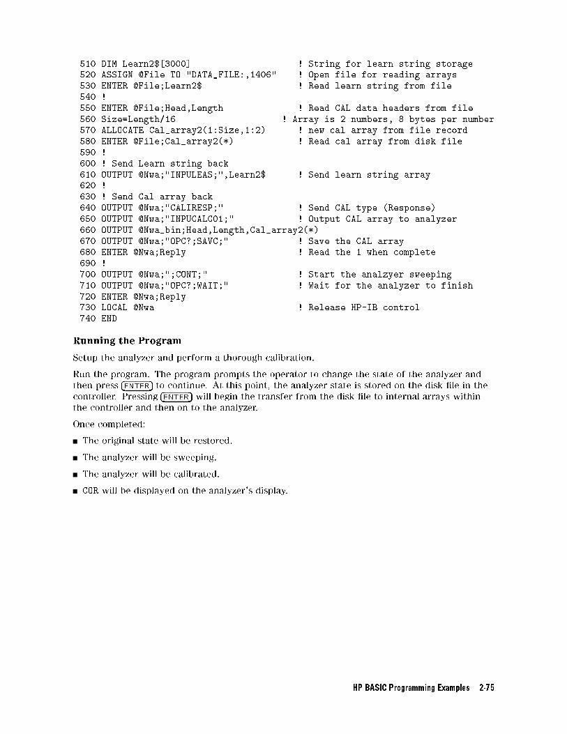
510 DIM Learn2$[3000] ! String for learn string storage
520 ASSIGN @File TO "DATA_FILE:,1406" ! Open file for reading arrays
530 ENTER @File;Learn2$ ! Read learn string from file
540 !
550 ENTER @File;Head,Length ! Read CAL data headers from file
560 Size=Length/16 ! Array is 2 numbers, 8 bytes per number
570 ALLOCATE Cal_array2(1:Size,1:2) ! new cal array from file record
580 ENTER @File;Cal_array2(*) ! Read cal array from disk file
590 !
600 ! Send Learn string back
610 OUTPUT @Nwa;"INPULEAS;",Learn2$ ! Send learn string array
620 !
630 ! Send Cal array back
640 OUTPUT @Nwa;"CALIRESP;" ! Send CAL type (Response)
650 OUTPUT @Nwa;"INPUCALC01;" ! Output CAL array to analyzer
660 OUTPUT @Nwa_bin;Head,Length,Cal_array2(*)
670 OUTPUT @Nwa;"OPC?;SAVC;" ! Save the CAL array
680 ENTER @Nwa;Reply ! Read the 1 when complete
690 !
700 OUTPUT @Nwa;";CONT;" ! Start the analzyer sweeping
710 OUTPUT @Nwa;"OPC?;WAIT;" ! Wait for the analyzer to finish
720 ENTER @Nwa;Reply
730 LOCAL @Nwa ! Release HP-IB control
740 END
Running the Program
Setup the analyzer and perform a thorough calibration.
Run the program. The program prompts the operator to change the state of the analyzer and
then press �ENTER� to continue. At this point, the analyzer state is stored on the disk �le in the
controller. Pressing �ENTER� will begin the transfer from the disk �le to internal arrays within
the controller and then on to the analyzer.
Once completed:
The original state will be restored.
The analyzer will be sweeping.
The analyzer will be calibrated.
COR will be displayed on the analyzer's display.
HP BASIC Programming Examples 2-75
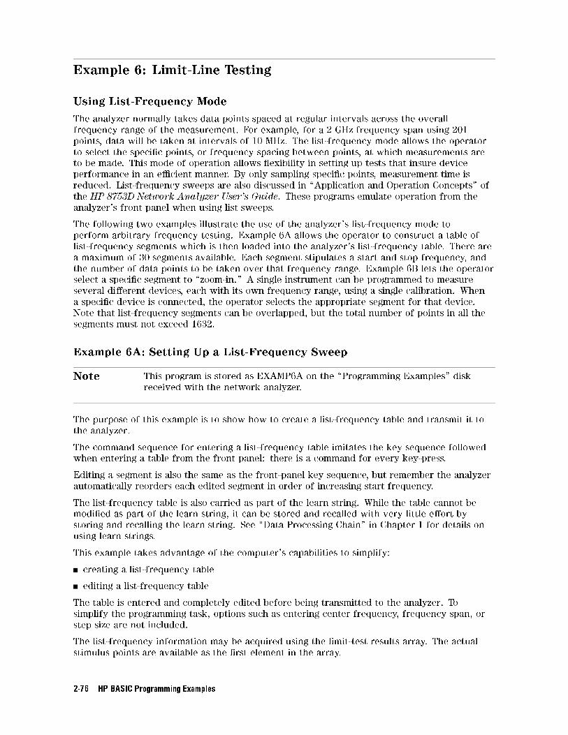
Example 6: Limit-Line Testing
Using List-Frequency Mode
The analyzer normally takes data points spaced at regular intervals across the overall
frequency range of the measurement. For example, for a 2 GHz frequency span using 201
points, data will be taken at intervals of 10 MHz. The list-frequency mode allows the operator
to select the speci�c points, or frequency spacing between points, at which measurements are
to be made. This mode of operation allows exibility in setting up tests that insure device
performance in an e�cient manner. By only sampling speci�c points, measurement time is
reduced. List-frequency sweeps are also discussed in \Application and Operation Concepts" of
the HP 8753D Network Analyzer User's Guide. These programs emulate operation from the
analyzer's front panel when using list sweeps.
The following two examples illustrate the use of the analyzer's list-frequency mode to
perform arbitrary frequency testing. Example 6A allows the operator to construct a table of
list-frequency segments which is then loaded into the analyzer's list-frequency table. There are
a maximum of 30 segments available. Each segment stipulates a start and stop frequency, and
the number of data points to be taken over that frequency range. Example 6B lets the operator
select a speci�c segment to \zoom-in." A single instrument can be programmed to measure
several di�erent devices, each with its own frequency range, using a single calibration. When
a speci�c device is connected, the operator selects the appropriate segment for that device.
Note that list-frequency segments can be overlapped, but the total number of points in all the
segments must not exceed 1632.
Example 6A: Setting Up a List-Frequency Sweep
Note This program is stored as EXAMP6A on the \Programming Examples" disk
received with the network analyzer.
The purpose of this example is to show how to create a list-frequency table and transmit it to
the analyzer.
The command sequence for entering a list-frequency table imitates the key sequence followed
when entering a table from the front panel: there is a command for every key-press.
Editing a segment is also the same as the front-panel key sequence, but remember the analyzer
automatically reorders each edited segment in order of increasing start frequency.
The list-frequency table is also carried as part of the learn string. While the table cannot be
modi�ed as part of the learn string, it can be stored and recalled with very little e�ort by
storing and recalling the learn string. See \Data Processing Chain" in Chapter 1 for details on
using learn strings.
This example takes advantage of the computer's capabilities to simplify:
creating a list-frequency table
editing a list-frequency table
The table is entered and completely edited before being transmitted to the analyzer. To
simplify the programming task, options such as entering center frequency, frequency span, or
step size are not included.
The list-frequency information may be acquired using the limit-test results array. The actual
stimulus points are available as the �rst element in the array.
2-76 HP BASIC Programming Examples
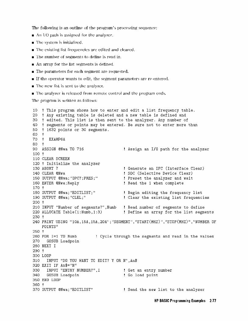
The following is an outline of the program's processing sequence:
An I/O path is assigned for the analyzer.
The system is initialized.
The existing list frequencies are edited and cleared.
The number of segments to de�ne is read in.
An array for the list segments is de�ned.
The parameters for each segment are requested.
If the operator wants to edit, the segment parameters are re-entered.
The new list is sent to the analyzer.
The analyzer is released from remote control and the program ends.
The program is written as follows:
10 ! This program shows how to enter and edit a list frequency table.
20 ! Any existing table is deleted and a new table is defined and
30 ! edited. This list is then sent to the analyzer. Any number of
40 ! segments or points may be entered. Be sure not to enter more than
50 ! 1632 points or 30 segments.
60 !
70 ! EXAMP6A
80 !
90 ASSIGN @Nwa TO 716 ! Assign an I/O path for the analyzer
100 !
110 CLEAR SCREEN
120 ! Initialize the analyzer
130 ABORT 7 ! Generate an IFC (Interface Clear)
140 CLEAR @Nwa ! SDC (Selective Device Clear)
150 OUTPUT @Nwa;"OPC?;PRES;" ! Preset the analyzer and wait
160 ENTER @Nwa;Reply ! Read the 1 when complete
170 !
180 OUTPUT @Nwa;"EDITLIST;" ! Begin editing the frequency list
190 OUTPUT @Nwa;"CLEL;" ! Clear the existing list frequencies
200 !
210 INPUT "Number of segments?",Numb ! Read number of segments to define
220 ALLOCATE Table(1:Numb,1:3) ! Define an array for the list segments
230 !
240 PRINT USING "10A,15A,15A,20A";"SEGMENT","START(MHZ)","STOP(MHZ)","NUMBER OF
POINTS"
250 !
260 FOR I=1 TO Numb ! Cycle through the segments and read in the values
270 GOSUB Loadpoin
280 NEXT I
290 !
300 LOOP
310 INPUT "DO YOU WANT TO EDIT? Y OR N",An$
320 EXIT IF An$="N"
330 INPUT "ENTRY NUMBER?",I ! Get an entry number
340 GOSUB Loadpoin ! Go load point
350 END LOOP
360 !
370 OUTPUT @Nwa;"EDITLIST" ! Send the new list to the analyzer
HP BASIC Programming Examples 2-77
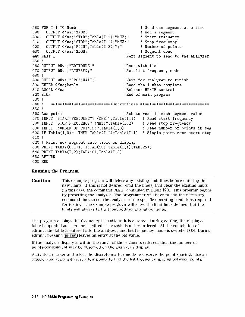
380 FOR I=1 TO Numb ! Send one segment at a time
390 OUTPUT @Nwa;"SADD;" ! Add a segment
400 OUTPUT @Nwa;"STAR";Table(I,1);"MHZ;" ! Start frequency
410 OUTPUT @Nwa;"STOP";Table(I,2);"MHZ;" ! Stop frequency
420 OUTPUT @Nwa;"POIN",Table(I,3),";" ! Number of points
430 OUTPUT @Nwa;"SDON;" ! Segment done
440 NEXT I ! Next segment to send to the analyzer
450 !
460 OUTPUT @Nwa;"EDITDONE;" ! Done with list
470 OUTPUT @Nwa;"LISFREQ;" ! Set list frequency mode
480 !
490 OUTPUT @Nwa;"OPC?;WAIT;" ! Wait for analyzer to finish
500 ENTER @Nwa;Reply ! Read the 1 when complete
510 LOCAL @Nwa ! Release HP-IB control
520 STOP ! End of main program
530 !
540 ! ***************************Subroutines ******************************
550 !
560 Loadpoin: ! Sub to read in each segment value
570 INPUT "START FREQUENCY? (MHZ)",Table(I,1) ! Read start frequency
580 INPUT "STOP FREQUENCY? (MHZ)",Table(I,2) ! Read stop frequency
590 INPUT "NUMBER OF POINTS?",Table(I,3) ! Read number of points in seg
600 IF Table(I,3)=1 THEN Table(I,2)=Table(I,1) ! Single point same start stop
610 !
620 ! Print new segment into table on display
630 PRINT TABXY(0,I+1);I;TAB(10);Table(I,1);TAB(25);
640 PRINT Table(I,2);TAB(40),Table(I,3)
650 RETURN
660 END
Running the Program
Caution This example program will delete any existing limit lines before entering the
new limits. If this is not desired, omit the line(s) that clear the existing limits
(in this case, the command CLEL; contained in LINE 190). This program begins
by presetting the analyzer. The programmer will have to add the necessary
command lines to set the analyzer to the speci�c operating conditions required
for testing. The example program will show the limit lines de�ned, but the
limits will always fail without additional analyzer setup.
The program displays the frequency-list table as it is entered. During editing, the displayed
table is updated as each line is edited. The table is not re-ordered. At the completion of
editing, the table is entered into the analyzer, and list-frequency mode is switched ON. During
editing, pressing �ENTER� leaves an entry at the old value.
If the analyzer display is within the range of the segments entered, then the number of
points-per-segment may be observed on the analyzer's display.
Activate a marker and select the discrete-marker mode to observe the point spacing. Use an
exaggerated scale with just a few points to �nd the list-frequency spacing between points.
2-78 HP BASIC Programming Examples
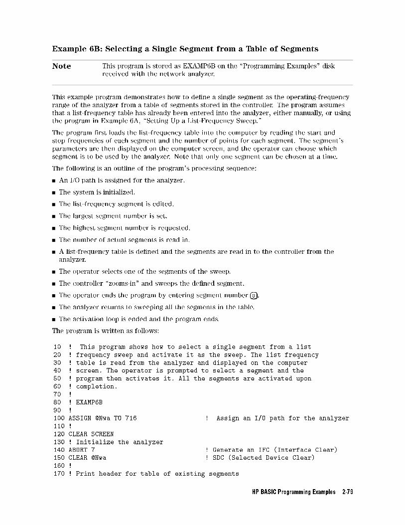
Example 6B: Selecting a Single Segment from a Table of Segments
Note This program is stored as EXAMP6B on the \Programming Examples" disk
received with the network analyzer.
This example program demonstrates how to de�ne a single segment as the operating-frequency
range of the analyzer from a table of segments stored in the controller. The program assumes
that a list-frequency table has already been entered into the analyzer, either manually, or using
the program in Example 6A, \Setting Up a List-Frequency Sweep."
The program �rst loads the list-frequency table into the computer by reading the start and
stop frequencies of each segment and the number of points for each segment. The segment's
parameters are then displayed on the computer screen, and the operator can choose which
segment is to be used by the analyzer. Note that only one segment can be chosen at a time.
The following is an outline of the program's processing sequence:
An I/O path is assigned for the analyzer.
The system is initialized.
The list-frequency segment is edited.
The largest segment number is set.
The highest segment number is requested.
The number of actual segments is read in.
A list-frequency table is de�ned and the segments are read in to the controller from the
analyzer.
The operator selects one of the segments of the sweep.
The controller \zooms-in" and sweeps the de�ned segment.
The operator ends the program by entering segment number �0�.
The analyzer returns to sweeping all the segments in the table.
The activation loop is ended and the program ends.
The program is written as follows:
10 ! This program shows how to select a single segment from a list
20 ! frequency sweep and activate it as the sweep. The list frequency
30 ! table is read from the analyzer and displayed on the computer
40 ! screen. The operator is prompted to select a segment and the
50 ! program then activates it. All the segments are activated upon
60 ! completion.
70 !
80 ! EXAMP6B
90 !
100 ASSIGN @Nwa TO 716 ! Assign an I/O path for the analyzer
110 !
120 CLEAR SCREEN
130 ! Initialize the analyzer
140 ABORT 7 ! Generate an IFC (Interface Clear)
150 CLEAR @Nwa ! SDC (Selected Device Clear)
160 !
170 ! Print header for table of existing segments
HP BASIC Programming Examples 2-79
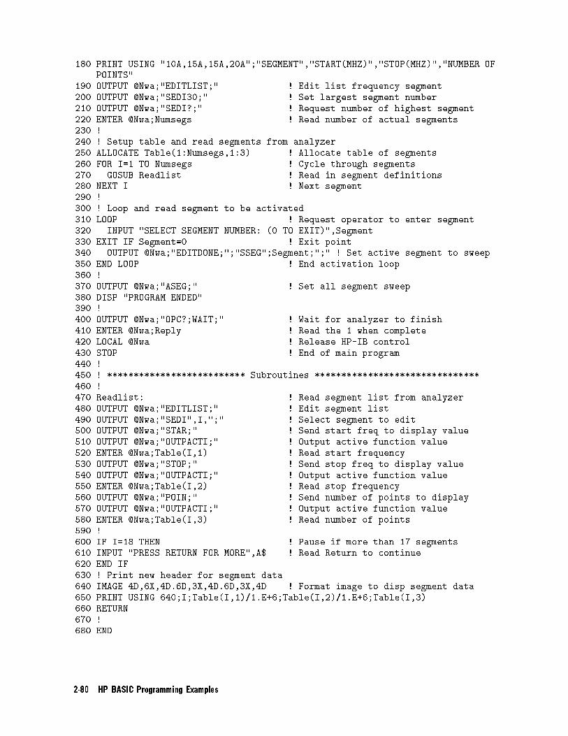
180 PRINT USING "10A,15A,15A,20A";"SEGMENT","START(MHZ)","STOP(MHZ)","NUMBER OF
POINTS"
190 OUTPUT @Nwa;"EDITLIST;" ! Edit list frequency segment
200 OUTPUT @Nwa;"SEDI30;" ! Set largest segment number
210 OUTPUT @Nwa;"SEDI?;" ! Request number of highest segment
220 ENTER @Nwa;Numsegs ! Read number of actual segments
230 !
240 ! Setup table and read segments from analyzer
250 ALLOCATE Table(1:Numsegs,1:3) ! Allocate table of segments
260 FOR I=1 TO Numsegs ! Cycle through segments
270 GOSUB Readlist ! Read in segment definitions
280 NEXT I ! Next segment
290 !
300 ! Loop and read segment to be activated
310 LOOP ! Request operator to enter segment
320 INPUT "SELECT SEGMENT NUMBER: (0 TO EXIT)",Segment
330 EXIT IF Segment=0 ! Exit point
340 OUTPUT @Nwa;"EDITDONE;";"SSEG";Segment;";" ! Set active segment to sweep
350 END LOOP ! End activation loop
360 !
370 OUTPUT @Nwa;"ASEG;" ! Set all segment sweep
380 DISP "PROGRAM ENDED"
390 !
400 OUTPUT @Nwa;"OPC?;WAIT;" ! Wait for analyzer to finish
410 ENTER @Nwa;Reply ! Read the 1 when complete
420 LOCAL @Nwa ! Release HP-IB control
430 STOP ! End of main program
440 !
450 ! ************************** Subroutines *******************************
460 !
470 Readlist: ! Read segment list from analyzer
480 OUTPUT @Nwa;"EDITLIST;" ! Edit segment list
490 OUTPUT @Nwa;"SEDI",I,";" ! Select segment to edit
500 OUTPUT @Nwa;"STAR;" ! Send start freq to display value
510 OUTPUT @Nwa;"OUTPACTI;" ! Output active function value
520 ENTER @Nwa;Table(I,1) ! Read start frequency
530 OUTPUT @Nwa;"STOP;" ! Send stop freq to display value
540 OUTPUT @Nwa;"OUTPACTI;" ! Output active function value
550 ENTER @Nwa;Table(I,2) ! Read stop frequency
560 OUTPUT @Nwa;"POIN;" ! Send number of points to display
570 OUTPUT @Nwa;"OUTPACTI;" ! Output active function value
580 ENTER @Nwa;Table(I,3) ! Read number of points
590 !
600 IF I=18 THEN ! Pause if more than 17 segments
610 INPUT "PRESS RETURN FOR MORE",A$ ! Read Return to continue
620 END IF
630 ! Print new header for segment data
640 IMAGE 4D,6X,4D.6D,3X,4D.6D,3X,4D ! Format image to disp segment data
650 PRINT USING 640;I;Table(I,1)/1.E+6;Table(I,2)/1.E+6;Table(I,3)
660 RETURN
670 !
680 END
2-80 HP BASIC Programming Examples
Running the Program
The program will read the parameters for each list-frequency segment from the analyzer, and
build a table containing all the segments. The parameters of each segment will be printed
on the computer screen. If there are more than 17 segments, the program will pause. Press
�RETURN� to see more segments. The maximum number of segments that can be read is 30
(the maximum number of segments the analyzer can hold). Use the computer's �Page Up� and�Page Down� keys to scroll through the list of segments if there are more than 17.
After all the segments are displayed, the program will prompt the operator for a speci�c
segment to be used. Type in the number of the segment, and the analyzer will then \zoom-in"
on that segment. The program will continue looping, allowing continuous selection of di�erent
segments. To exit the loop, type �0�. This will restore all the segments (with the command
ASEG), allowing the analyzer to sweep all of the segments, and the program will terminate.
Using Limit Lines to Perform PASS/FAIL Tests
There are two steps to performing limit testing on the analyzer via HP-IB. First, limit
speci�cations must be de�ned and loaded into the analyzer. Second, the limits are activated,
the device is measured, and its performance to the speci�ed limits is signaled by a pass or fail
message on the analyzer's display.
Example 6C illustrates the �rst step, setting up limits. Example 6D performs the actual limit
testing.
HP BASIC Programming Examples 2-81
Example 6C: Setting Up Limit Lines
Note This program is stored as EXAMP6C on the \Programming Examples" disk
received with the network analyzer.
The purpose of this example is to show how to create a limit-test table and transmit it to the
analyzer.
The command sequence for entering a limit-test table imitates the key sequence followed when
entering a table from the analyzer's front panel: there is a command for every key-press.
Editing a limit line is also the same as the key sequence, but remember that the analyzer
automatically re-orders the table in order of increasing start frequency.
The limit-test table is also carried as part of the learn string. While it cannot be modi�ed as
part of the learn string, the learn string can be stored and recalled with very little e�ort. See
\Data-Processing Chain" in Chapter 1 for details on using learn strings.
This example takes advantage of the computer's capabilities to simplify creating and editing
the table. The table is entered and completely edited before being transmitted to the analyzer.
To simplify the programming task, options such as entering o�sets are not included.
This example automates the front-panel operation of entering a limit-test table. Front-panel
operation and limits are discussed in the \Application and Operation Concepts" in the
HP 8753D Network Analyzer User's Guide.
The following is an outline of the program's processing sequence:
An I/O path is assigned for the analyzer.
The system is initialized.
The limit lines are edited and cleared.
The number of limits is requested.
The limit table is created.
The string array of limit types is created.
The operator is prompted to enter the new limit values.
The new limit table is sent back to the analyzer.
The limit line is activated.
The limit test is activated.
The analyzer is returned to local control and the program ends.
The program is written as follows:
10 ! This program shows how to create a limit table and send it to the
20 ! analyzer. The operator enters the desired limits when prompted for
30 ! the stimulus value, upper and lower value and type of limit
40 ! desired. Once the table is created, the limits are sent to the
50 ! analyzer and activated.
60 !
70 ! EXAMP6C
80 !
90 ASSIGN @Nwa TO 716 ! Assign an I/O path for the analyzer
100 !
110 CLEAR SCREEN
2-82 HP BASIC Programming Examples
120 ! Initialize the analyzer
130 ABORT 7 ! Generate an IFC (Interface clear)
140 CLEAR @Nwa ! SDC (Selected Device Clear)
150 OUTPUT @Nwa;"OPC?;PRES;" ! Preset the analyzer and wait
160 ENTER @Nwa;Reply ! Read the 1 when completed
170 !
180 OUTPUT @Nwa;"EDITLIML;" ! Edit limit lines
190 OUTPUT @Nwa;"CLEL;" ! Clear any existing limits
200 INPUT "NUMBER OF LIMITS?",Numb ! Request the number of limits
210 ALLOCATE Table(1:Numb,1:3) ! Create a table
220 ALLOCATE Limtype$(Numb)[2] ! Create string array of limit types
230 !
240 ! Print out the header for the table
250 PRINT USING "10A,20A,15A,20A";"SEG","STIMULUS (MHz)","UPPER (dB)","
LOWER (dB)", "TYPE"
260 !
270 ! Prompt the operator to enter the limit values
280 FOR I=1 TO Numb ! Cycle through the limits
290 GOSUB Loadlimit ! Go read limit values
300 NEXT I ! Next limit value
310 !
320 ! Allow the operator to edit the array entered
330 LOOP ! Cycle to edit limit lines
340 INPUT "DO YOU WANT TO EDIT? Y OR N",An$
350 EXIT IF An$="N" ! Exit loop on N and send to analyzer
360 INPUT "ENTRY NUMBER?",I ! Read limit number to edit
370 GOSUB Loadlimit ! Go read limit values
380 END LOOP ! Next edit entry
390 !
400 ! Send the limit line array segments to the analyzer
410 OUTPUT @Nwa;"EDITLIML;" ! Edit the limit
420 FOR I=1 TO Numb ! Each segment of the limit
430 OUTPUT @Nwa;"SADD;" ! Add segment
440 OUTPUT @Nwa;"LIMS";Table(I,1);"MHZ" ! Send segment stimulus value
450 OUTPUT @Nwa;"LIMU";Table(I,2);"DB" ! Upper limit value
460 OUTPUT @Nwa;"LIML";Table(I,3);"DB" ! Lower limit value
470 IF Limtype$(I)="FL" THEN OUTPUT @Nwa;"LIMTFL;" ! Flat limit
480 IF Limtype$(I)="SL" THEN OUTPUT @Nwa;"LIMTSL;" ! Sloping limit
490 IF Limtype$(I)="SP" THEN OUTPUT @Nwa;"LIMTSP;" ! Point limit
500 OUTPUT @Nwa;"SDON;" ! Segment done
510 NEXT I ! next segment
520 !
530 OUTPUT @Nwa;"EDITDONE;" ! Edit complete
540 OUTPUT @Nwa;"LIMILINEON;" ! Turn limit line on
550 OUTPUT @Nwa;"LIMITESTON;" ! Turn limit test on
560 !
570 OUTPUT @Nwa;"OPC?;WAIT;" ! Wait for the analyzer to finish
580 ENTER @Nwa;Reply ! Read the 1 when complete
590 !
600 LOCAL @Nwa ! Release HP-IB control
610 STOP ! End of main program
620 !
630 !************************** Subroutines ******************************
640 !
650 Loadlimit: ! Sub to interact to load data
HP BASIC Programming Examples 2-83
660 INPUT "STIMULUS VALUE? (MHz)",Table(I,1) ! and print table created
670 INPUT "UPPER LIMIT VALUE? (DB)",Table(I,2)
680 INPUT "LOWER LIMIT VALUE? (DB)",Table(I,3)
690 INPUT "LIMIT TYPE? (FL=FLAT, SL=SLOPED, SP=SINGLE POINT)",Limtype$(I)
700 !
710 ! Format and display table values
720 PRINT TABXY(0,I+1);I;TAB(10);Table(I,1);TAB(30);Table(I,2);TAB(45),
Table(I,3),TAB(67);Limtype$(I)
730 RETURN ! Next limit value
740 !
750 END
Running the Program
Caution This example program will delete any existing limit lines before entering
the new limits. If this is not desired, omit the line(s) that clear the existing
limits (in this case, the command "CLEL;" contained in LINE 190). This
program begins by presetting the analyzer. The programmer will have to add
the necessary command lines to set the analyzer to the operating conditions
required for testing. The example program will show the limit lines de�ned,
but the limits will always fail without additional analyzer setup.
The program displays the limit table as it is entered. During editing, the displayed table is
updated as each line is edited. The table is not reordered. At the completion of editing, the
table is entered into the analyzer, and limit-testing mode switched ON. The analyzer will
rearrange the table in ascending order starting with the lowest start frequency entry. During
editing, simply pressing �ENTER� leaves an entry at the old value.
2-84 HP BASIC Programming Examples
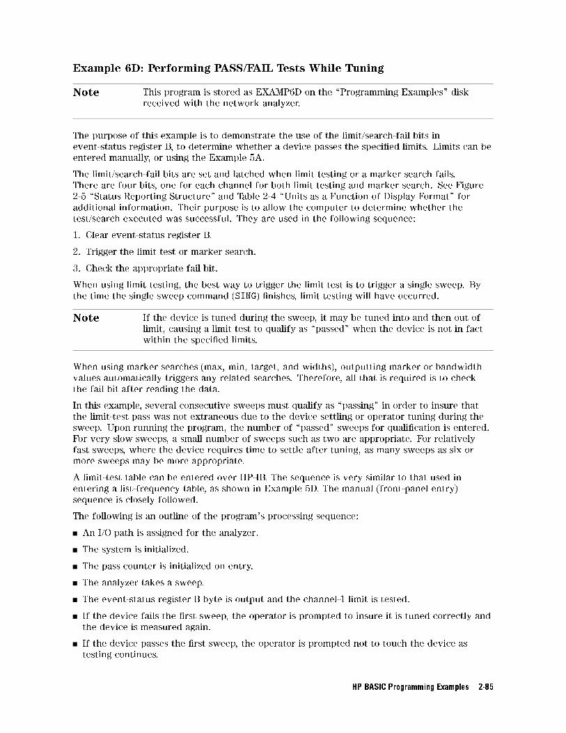
Example 6D: Performing PASS/FAIL Tests While Tuning
Note This program is stored as EXAMP6D on the \Programming Examples" disk
received with the network analyzer.
The purpose of this example is to demonstrate the use of the limit/search-fail bits in
event-status register B, to determine whether a device passes the speci�ed limits. Limits can be
entered manually, or using the Example 5A.
The limit/search-fail bits are set and latched when limit testing or a marker search fails.
There are four bits, one for each channel for both limit testing and marker search. See Figure
2-5 \Status Reporting Structure" and Table 2-4 \Units as a Function of Display Format" for
additional information. Their purpose is to allow the computer to determine whether the
test/search executed was successful. They are used in the following sequence:
1. Clear event-status register B.
2. Trigger the limit test or marker search.
3. Check the appropriate fail bit.
When using limit testing, the best way to trigger the limit test is to trigger a single sweep. By
the time the single sweep command (SING) �nishes, limit testing will have occurred.
Note If the device is tuned during the sweep, it may be tuned into and then out of
limit, causing a limit test to qualify as \passed" when the device is not in fact
within the speci�ed limits.
When using marker searches (max, min, target, and widths), outputting marker or bandwidth
values automatically triggers any related searches. Therefore, all that is required is to check
the fail bit after reading the data.
In this example, several consecutive sweeps must qualify as \passing" in order to insure that
the limit-test pass was not extraneous due to the device settling or operator tuning during the
sweep. Upon running the program, the number of \passed" sweeps for quali�cation is entered.
For very slow sweeps, a small number of sweeps such as two are appropriate. For relatively
fast sweeps, where the device requires time to settle after tuning, as many sweeps as six or
more sweeps may be more appropriate.
A limit-test table can be entered over HP-IB. The sequence is very similar to that used in
entering a list-frequency table, as shown in Example 5D. The manual (front-panel entry)
sequence is closely followed.
The following is an outline of the program's processing sequence:
An I/O path is assigned for the analyzer.
The system is initialized.
The pass counter is initialized on entry.
The analyzer takes a sweep.
The event-status register B byte is output and the channel-1 limit is tested.
If the device fails the �rst sweep, the operator is prompted to insure it is tuned correctly and
the device is measured again.
If the device passes the �rst sweep, the operator is prompted not to touch the device as
testing continues.
HP BASIC Programming Examples 2-85
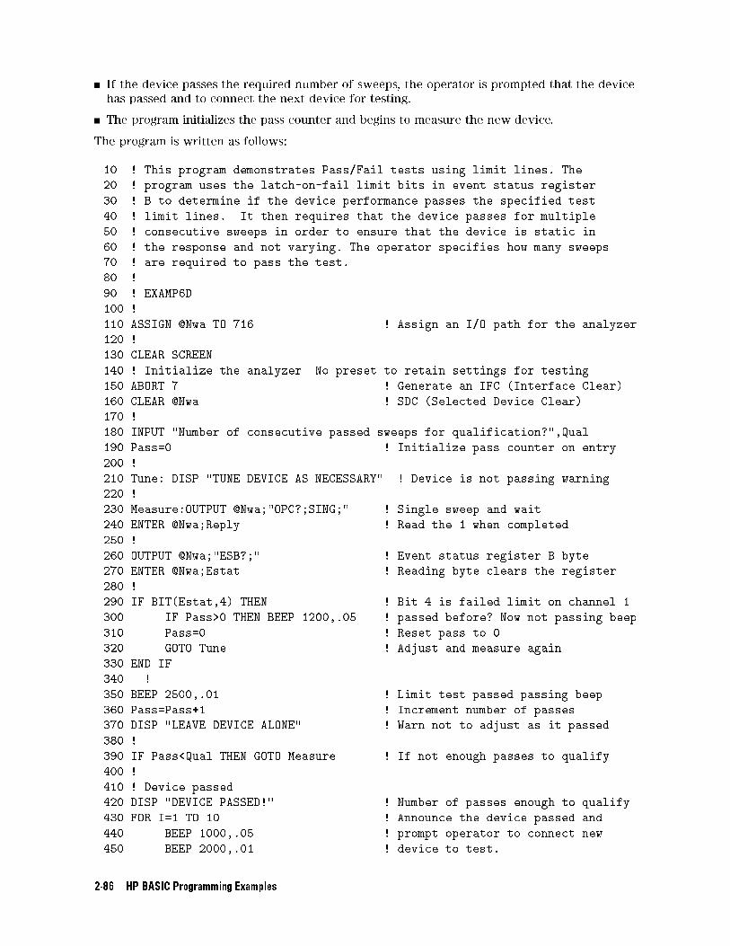
If the device passes the required number of sweeps, the operator is prompted that the device
has passed and to connect the next device for testing.
The program initializes the pass counter and begins to measure the new device.
The program is written as follows:
10 ! This program demonstrates Pass/Fail tests using limit lines. The
20 ! program uses the latch-on-fail limit bits in event status register
30 ! B to determine if the device performance passes the specified test
40 ! limit lines. It then requires that the device passes for multiple
50 ! consecutive sweeps in order to ensure that the device is static in
60 ! the response and not varying. The operator specifies how many sweeps
70 ! are required to pass the test.
80 !
90 ! EXAMP6D
100 !
110 ASSIGN @Nwa TO 716 ! Assign an I/O path for the analyzer
120 !
130 CLEAR SCREEN
140 ! Initialize the analyzer No preset to retain settings for testing
150 ABORT 7 ! Generate an IFC (Interface Clear)
160 CLEAR @Nwa ! SDC (Selected Device Clear)
170 !
180 INPUT "Number of consecutive passed sweeps for qualification?",Qual
190 Pass=0 ! Initialize pass counter on entry
200 !
210 Tune: DISP "TUNE DEVICE AS NECESSARY" ! Device is not passing warning
220 !
230 Measure:OUTPUT @Nwa;"OPC?;SING;" ! Single sweep and wait
240 ENTER @Nwa;Reply ! Read the 1 when completed
250 !
260 OUTPUT @Nwa;"ESB?;" ! Event status register B byte
270 ENTER @Nwa;Estat ! Reading byte clears the register
280 !
290 IF BIT(Estat,4) THEN ! Bit 4 is failed limit on channel 1
300 IF Pass>0 THEN BEEP 1200,.05 ! passed before? Now not passing beep
310 Pass=0 ! Reset pass to 0
320 GOTO Tune ! Adjust and measure again
330 END IF
340 !
350 BEEP 2500,.01 ! Limit test passed passing beep
360 Pass=Pass+1 ! Increment number of passes
370 DISP "LEAVE DEVICE ALONE" ! Warn not to adjust as it passed
380 !
390 IF Pass<Qual THEN GOTO Measure ! If not enough passes to qualify
400 !
410 ! Device passed
420 DISP "DEVICE PASSED!" ! Number of passes enough to qualify
430 FOR I=1 TO 10 ! Announce the device passed and
440 BEEP 1000,.05 ! prompt operator to connect new
450 BEEP 2000,.01 ! device to test.
2-86 HP BASIC Programming Examples
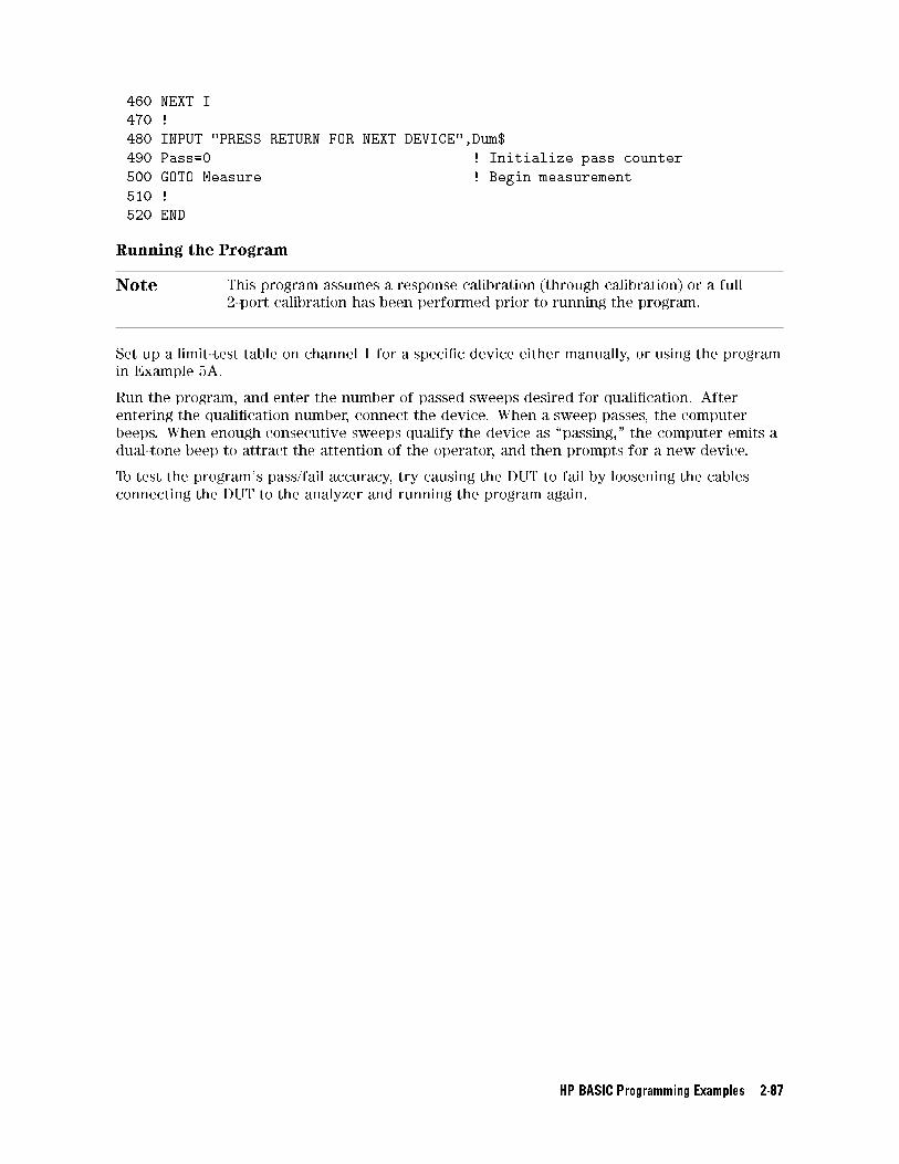
460 NEXT I
470 !
480 INPUT "PRESS RETURN FOR NEXT DEVICE",Dum$
490 Pass=0 ! Initialize pass counter
500 GOTO Measure ! Begin measurement
510 !
520 END
Running the Program
Note This program assumes a response calibration (through calibration) or a full
2-port calibration has been performed prior to running the program.
Set up a limit-test table on channel 1 for a speci�c device either manually, or using the program
in Example 5A.
Run the program, and enter the number of passed sweeps desired for quali�cation. After
entering the quali�cation number, connect the device. When a sweep passes, the computer
beeps. When enough consecutive sweeps qualify the device as \passing," the computer emits a
dual-tone beep to attract the attention of the operator, and then prompts for a new device.
To test the program's pass/fail accuracy, try causing the DUT to fail by loosening the cables
connecting the DUT to the analyzer and running the program again.
HP BASIC Programming Examples 2-87
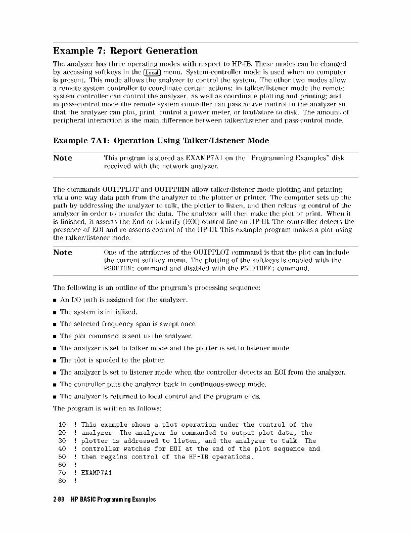
Example 7: Report Generation
The analyzer has three operating modes with respect to HP-IB. These modes can be changed
by accessing softkeys in the �Local� menu. System-controller mode is used when no computer
is present. This mode allows the analyzer to control the system. The other two modes allow
a remote system controller to coordinate certain actions: in talker/listener mode the remote
system controller can control the analyzer, as well as coordinate plotting and printing; and
in pass-control mode the remote system controller can pass active control to the analyzer so
that the analyzer can plot, print, control a power meter, or load/store to disk. The amount of
peripheral interaction is the main di�erence between talker/listener and pass-control mode.
Example 7A1: Operation Using Talker/Listener Mode
Note This program is stored as EXAMP7A1 on the \Programming Examples" disk
received with the network analyzer.
The commands OUTPPLOT and OUTPPRIN allow talker/listener mode plotting and printing
via a one way data path from the analyzer to the plotter or printer. The computer sets up the
path by addressing the analyzer to talk, the plotter to listen, and then releasing control of the
analyzer in order to transfer the data. The analyzer will then make the plot or print. When it
is �nished, it asserts the End or Identify (EOI) control line on HP-IB. The controller detects the
presence of EOI and re-asserts control of the HP-IB. This example program makes a plot using
the talker/listener mode.
Note One of the attributes of the OUTPPLOT command is that the plot can include
the current softkey menu. The plotting of the softkeys is enabled with the
PSOFTON; command and disabled with the PSOFTOFF; command.
The following is an outline of the program's processing sequence:
An I/O path is assigned for the analyzer.
The system is initialized.
The selected frequency span is swept once.
The plot command is sent to the analyzer.
The analyzer is set to talker mode and the plotter is set to listener mode.
The plot is spooled to the plotter.
The analyzer is set to listener mode when the controller detects an EOI from the analyzer.
The controller puts the analyzer back in continuous-sweep mode.
The analyzer is returned to local control and the program ends.
The program is written as follows:
10 ! This example shows a plot operation under the control of the
20 ! analyzer. The analyzer is commanded to output plot data, the
30 ! plotter is addressed to listen, and the analyzer to talk. The
40 ! controller watches for EOI at the end of the plot sequence and
50 ! then regains control of the HP-IB operations.
60 !
70 ! EXAMP7A1
80 !
2-88 HP BASIC Programming Examples
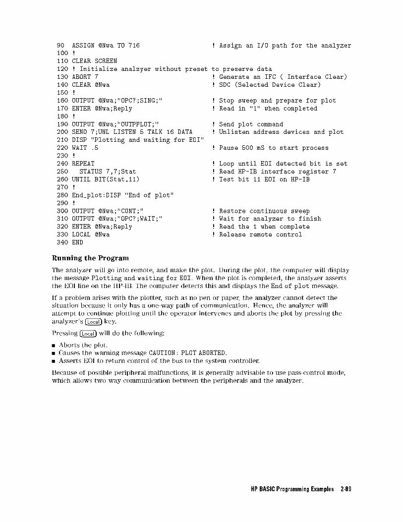
90 ASSIGN @Nwa TO 716 ! Assign an I/O path for the analyzer
100 !
110 CLEAR SCREEN
120 ! Initialize analzyer without preset to preserve data
130 ABORT 7 ! Generate an IFC ( Interface Clear)
140 CLEAR @Nwa ! SDC (Selected Device Clear)
150 !
160 OUTPUT @Nwa;"OPC?;SING;" ! Stop sweep and prepare for plot
170 ENTER @Nwa;Reply ! Read in "1" when completed
180 !
190 OUTPUT @Nwa;"OUTPPLOT;" ! Send plot command
200 SEND 7;UNL LISTEN 5 TALK 16 DATA ! Unlisten address devices and plot
210 DISP "Plotting and waiting for EOI"
220 WAIT .5 ! Pause 500 mS to start process
230 !
240 REPEAT ! Loop until EOI detected bit is set
250 STATUS 7,7;Stat ! Read HP-IB interface register 7
260 UNTIL BIT(Stat,11) ! Test bit 11 EOI on HP-IB
270 !
280 End_plot:DISP "End of plot"
290 !
300 OUTPUT @Nwa;"CONT;" ! Restore continuous sweep
310 OUTPUT @Nwa;"OPC?;WAIT;" ! Wait for analyzer to finish
320 ENTER @Nwa;Reply ! Read the 1 when complete
330 LOCAL @Nwa ! Release remote control
340 END
Running the Program
The analyzer will go into remote, and make the plot. During the plot, the computer will display
the message Plotting and waiting for EOI. When the plot is completed, the analyzer asserts
the EOI line on the HP-IB. The computer detects this and displays the End of plot message.
If a problem arises with the plotter, such as no pen or paper, the analyzer cannot detect the
situation because it only has a one-way path of communication. Hence, the analyzer will
attempt to continue plotting until the operator intervenes and aborts the plot by pressing the
analyzer's �Local� key.
Pressing �Local� will do the following:
Aborts the plot.
Causes the warning message CAUTION: PLOT ABORTED.
Asserts EOI to return control of the bus to the system controller.
Because of possible peripheral malfunctions, it is generally advisable to use pass-control mode,
which allows two way communication between the peripherals and the analyzer.
HP BASIC Programming Examples 2-89
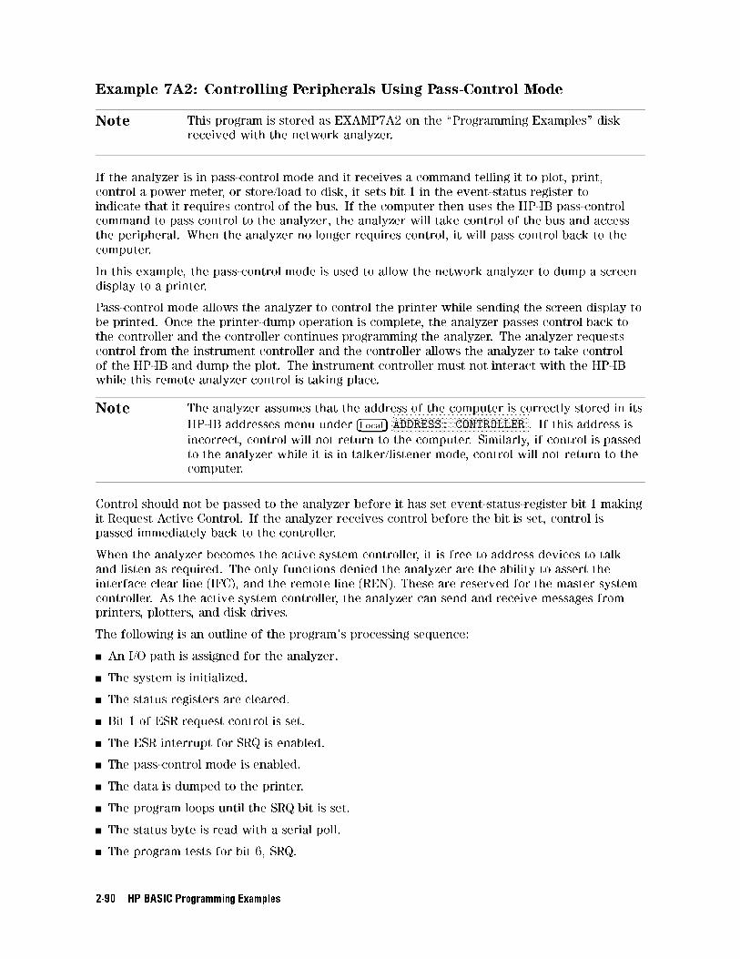
Example 7A2: Controlling Peripherals Using Pass-Control Mode
Note This program is stored as EXAMP7A2 on the \Programming Examples" disk
received with the network analyzer.
If the analyzer is in pass-control mode and it receives a command telling it to plot, print,
control a power meter, or store/load to disk, it sets bit 1 in the event-status register to
indicate that it requires control of the bus. If the computer then uses the HP-IB pass-control
command to pass control to the analyzer, the analyzer will take control of the bus and access
the peripheral. When the analyzer no longer requires control, it will pass control back to the
computer.
In this example, the pass-control mode is used to allow the network analyzer to dump a screen
display to a printer.
Pass-control mode allows the analyzer to control the printer while sending the screen display to
be printed. Once the printer-dump operation is complete, the analyzer passes control back to
the controller and the controller continues programming the analyzer. The analyzer requests
control from the instrument controller and the controller allows the analyzer to take control
of the HP-IB and dump the plot. The instrument controller must not interact with the HP-IB
while this remote analyzer control is taking place.
Note The analyzer assumes that the address of the computer is correctly stored in its
HP-IB addresses menu under �Local�NNNNNNNNNNNNNNNNNNNNNNNNNNNNNNNNNNNNNNNNNNNNNNNNNNNNNNNNNNNADDRESS: CONTROLLER . If this address is
incorrect, control will not return to the computer. Similarly, if control is passed
to the analyzer while it is in talker/listener mode, control will not return to the
computer.
Control should not be passed to the analyzer before it has set event-status-register bit 1 making
it Request Active Control. If the analyzer receives control before the bit is set, control is
passed immediately back to the controller.
When the analyzer becomes the active system controller, it is free to address devices to talk
and listen as required. The only functions denied the analyzer are the ability to assert the
interface clear line (IFC), and the remote line (REN). These are reserved for the master system
controller. As the active system controller, the analyzer can send and receive messages from
printers, plotters, and disk drives.
The following is an outline of the program's processing sequence:
An I/O path is assigned for the analyzer.
The system is initialized.
The status registers are cleared.
Bit 1 of ESR request control is set.
The ESR interrupt for SRQ is enabled.
The pass-control mode is enabled.
The data is dumped to the printer.
The program loops until the SRQ bit is set.
The status byte is read with a serial poll.
The program tests for bit 6, SRQ.
2-90 HP BASIC Programming Examples
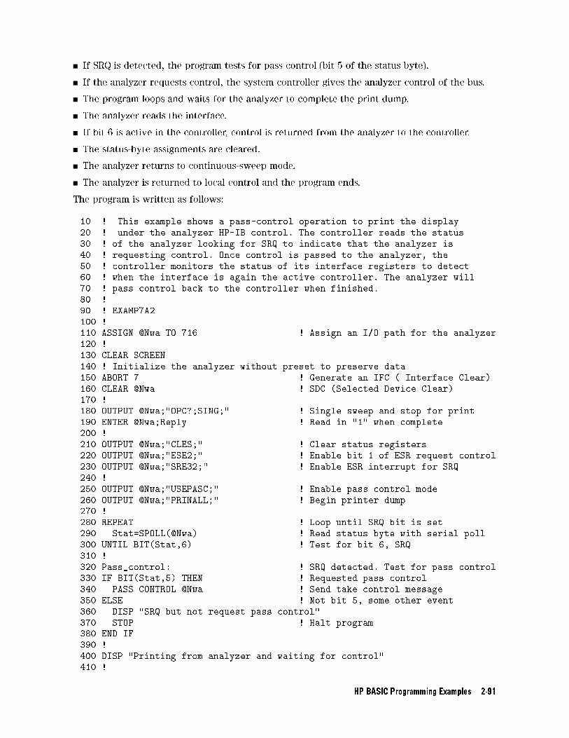
If SRQ is detected, the program tests for pass control (bit 5 of the status byte).
If the analyzer requests control, the system controller gives the analyzer control of the bus.
The program loops and waits for the analyzer to complete the print dump.
The analyzer reads the interface.
If bit 6 is active in the controller, control is returned from the analyzer to the controller.
The status-byte assignments are cleared.
The analyzer returns to continuous-sweep mode.
The analyzer is returned to local control and the program ends.
The program is written as follows:
10 ! This example shows a pass-control operation to print the display
20 ! under the analyzer HP-IB control. The controller reads the status
30 ! of the analyzer looking for SRQ to indicate that the analyzer is
40 ! requesting control. Once control is passed to the analyzer, the
50 ! controller monitors the status of its interface registers to detect
60 ! when the interface is again the active controller. The analyzer will
70 ! pass control back to the controller when finished.
80 !
90 ! EXAMP7A2
100 !
110 ASSIGN @Nwa TO 716 ! Assign an I/O path for the analyzer
120 !
130 CLEAR SCREEN
140 ! Initialize the analyzer without preset to preserve data
150 ABORT 7 ! Generate an IFC ( Interface Clear)
160 CLEAR @Nwa ! SDC (Selected Device Clear)
170 !
180 OUTPUT @Nwa;"OPC?;SING;" ! Single sweep and stop for print
190 ENTER @Nwa;Reply ! Read in "1" when complete
200 !
210 OUTPUT @Nwa;"CLES;" ! Clear status registers
220 OUTPUT @Nwa;"ESE2;" ! Enable bit 1 of ESR request control
230 OUTPUT @Nwa;"SRE32;" ! Enable ESR interrupt for SRQ
240 !
250 OUTPUT @Nwa;"USEPASC;" ! Enable pass control mode
260 OUTPUT @Nwa;"PRINALL;" ! Begin printer dump
270 !
280 REPEAT ! Loop until SRQ bit is set
290 Stat=SPOLL(@Nwa) ! Read status byte with serial poll
300 UNTIL BIT(Stat,6) ! Test for bit 6, SRQ
310 !
320 Pass_control: ! SRQ detected. Test for pass control
330 IF BIT(Stat,5) THEN ! Requested pass control
340 PASS CONTROL @Nwa ! Send take control message
350 ELSE ! Not bit 5, some other event
360 DISP "SRQ but not request pass control"
370 STOP ! Halt program
380 END IF
390 !
400 DISP "Printing from analyzer and waiting for control"
410 !
HP BASIC Programming Examples 2-91
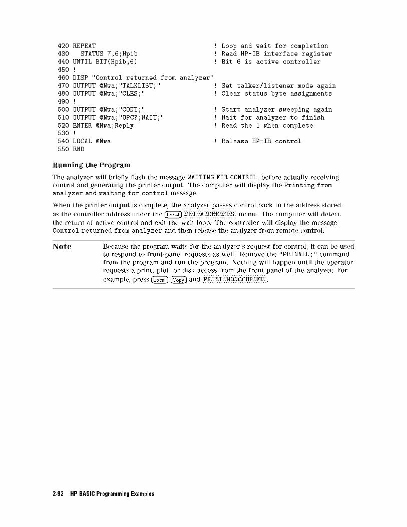
420 REPEAT ! Loop and wait for completion
430 STATUS 7,6;Hpib ! Read HP-IB interface register
440 UNTIL BIT(Hpib,6) ! Bit 6 is active controller
450 !
460 DISP "Control returned from analyzer"
470 OUTPUT @Nwa;"TALKLIST;" ! Set talker/listener mode again
480 OUTPUT @Nwa;"CLES;" ! Clear status byte assignments
490 !
500 OUTPUT @Nwa;"CONT;" ! Start analyzer sweeping again
510 OUTPUT @Nwa;"OPC?;WAIT;" ! Wait for analyzer to finish
520 ENTER @Nwa;Reply ! Read the 1 when complete
530 !
540 LOCAL @Nwa ! Release HP-IB control
550 END
Running the Program
The analyzer will brie y ash the message WAITING FOR CONTROL, before actually receiving
control and generating the printer output. The computer will display the Printing from
analyzer and waiting for control message.
When the printer output is complete, the analyzer passes control back to the address stored
as the controller address under the �Local�NNNNNNNNNNNNNNNNNNNNNNNNNNNNNNNNNNNNNNNNNSET ADDRESSES menu. The computer will detect
the return of active control and exit the wait loop. The controller will display the message
Control returned from analyzer and then release the analyzer from remote control.
Note Because the program waits for the analyzer's request for control, it can be used
to respond to front-panel requests as well. Remove the "PRINALL;" command
from the program and run the program. Nothing will happen until the operator
requests a print, plot, or disk access from the front panel of the analyzer. For
example, press �Local� �Copy� andNNNNNNNNNNNNNNNNNNNNNNNNNNNNNNNNNNNNNNNNNNNNNNNNNNPRINT MONOCHROME .
2-92 HP BASIC Programming Examples
Example 7A3: Printing with the Serial Port
Note This program is stored as EXAMP7A3 on the \Programming Examples" disk
received with the network analyzer.
This program will select the serial port and program the analyzer to copy its display to a
printer. There are a number of commands associated with the serial and parallel ports which
allow the programmer to con�gure the output modes, for example the baud rate and the
handshake type used by the port and the printer. In this example, the serial port is con�gured
by the program. The interface may also be con�gured from the analyzer's front-panel keys
by pressing �Local�NNNNNNNNNNNNNNNNNNNNNNNNNNNNNNNNNNNNNNNNNSET ADDRESSES
NNNNNNNNNNNNNNNNNNNNNNNNNNNNNNNNNNNNNNPRINTER PORT . This menu allows manual selection of the
serial-interface parameters.
Since the HP-IB port is not being used for the copy operation, programming of the analyzer
and measurement operations may continue once the copy operation has been initiated. An
internal spooler in the analyzer's memory provides bu�ering of the printer operation. In the
example which follows, the status byte of the analyzer is checked to determine when the print
operation is complete.
An I/O path is assigned to the analyzer.
The analyzer is initialized.
A single sweep is taken and the analyzer is placed in hold mode.
The status registers are cleared.
The copy-complete bit is set and enabled.
The printer operation and communication modes are set.
The print command is sent.
The analyzer is released from remote control and placed in continuous-sweep mode.
The analyzer is polled until the status bit representing copy complete is detected.
The analyzer is released from remote control and the program ends.
HP BASIC Programming Examples 2-93
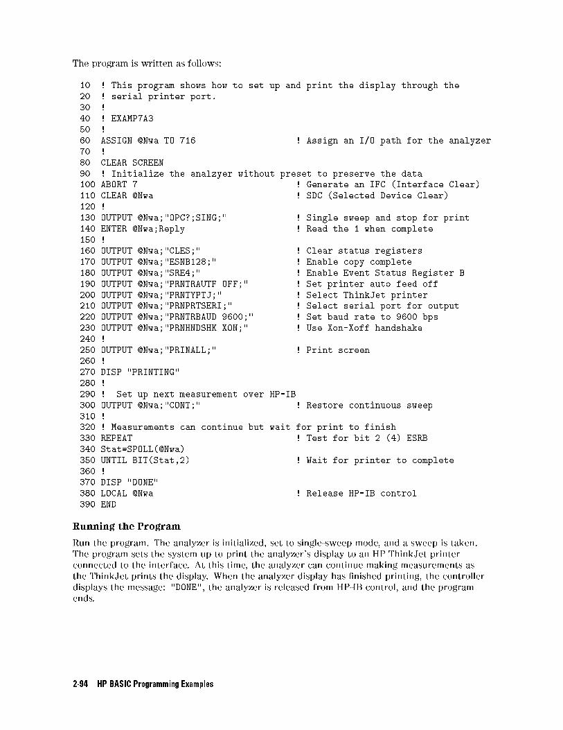
The program is written as follows:
10 ! This program shows how to set up and print the display through the
20 ! serial printer port.
30 !
40 ! EXAMP7A3
50 !
60 ASSIGN @Nwa TO 716 ! Assign an I/O path for the analyzer
70 !
80 CLEAR SCREEN
90 ! Initialize the analzyer without preset to preserve the data
100 ABORT 7 ! Generate an IFC (Interface Clear)
110 CLEAR @Nwa ! SDC (Selected Device Clear)
120 !
130 OUTPUT @Nwa;"OPC?;SING;" ! Single sweep and stop for print
140 ENTER @Nwa;Reply ! Read the 1 when complete
150 !
160 OUTPUT @Nwa;"CLES;" ! Clear status registers
170 OUTPUT @Nwa;"ESNB128;" ! Enable copy complete
180 OUTPUT @Nwa;"SRE4;" ! Enable Event Status Register B
190 OUTPUT @Nwa;"PRNTRAUTF OFF;" ! Set printer auto feed off
200 OUTPUT @Nwa;"PRNTYPTJ;" ! Select ThinkJet printer
210 OUTPUT @Nwa;"PRNPRTSERI;" ! Select serial port for output
220 OUTPUT @Nwa;"PRNTRBAUD 9600;" ! Set baud rate to 9600 bps
230 OUTPUT @Nwa;"PRNHNDSHK XON;" ! Use Xon-Xoff handshake
240 !
250 OUTPUT @Nwa;"PRINALL;" ! Print screen
260 !
270 DISP "PRINTING"
280 !
290 ! Set up next measurement over HP-IB
300 OUTPUT @Nwa;"CONT;" ! Restore continuous sweep
310 !
320 ! Measurements can continue but wait for print to finish
330 REPEAT ! Test for bit 2 (4) ESRB
340 Stat=SPOLL(@Nwa)
350 UNTIL BIT(Stat,2) ! Wait for printer to complete
360 !
370 DISP "DONE"
380 LOCAL @Nwa ! Release HP-IB control
390 END
Running the Program
Run the program. The analyzer is initialized, set to single-sweep mode, and a sweep is taken.
The program sets the system up to print the analyzer's display to an HP ThinkJet printer
connected to the interface. At this time, the analyzer can continue making measurements as
the ThinkJet prints the display. When the analyzer display has �nished printing, the controller
displays the message: "DONE", the analyzer is released from HP-IB control, and the program
ends.
2-94 HP BASIC Programming Examples
Example 7B: Plotting to a File and Transferring the File Data to a Plotter
Note This program is stored as EXAMP7B on the \Programming Examples" disk
received with the network analyzer.
Another report-generation technique is to transfer the plotter string to a disk �le, and retrieve
and plot the disk �le at another time. Test time is increased when a hardcopy plot occurs
during the measurement process. It may be more convenient to plot the data at another site or
time. One solution to this problem is to capture the plot data using the controller and store it to
a disk �le. This disk �le may then be read from the controller and the contents transferred to a
plotter. This next example shows a method of accomplishing this task.
The analyzer is initialized without presetting the analyzer. The data that is in place on the
analyzer is not disturbed by the program operation. A large string is dimensioned to hold the
plotter commands as they are received from the analyzer. The length of this string depends
upon the complexity of the analyzer's display. The analyzer is placed in the single-sweep mode
and OPC?;SING; is used to make sure that operation is complete before plotting. The plotting
begins with the OUTPPLOT; command.
The string transfer is ended by the controller detecting the EOI line which the analyzer pulls
at the end of the transfer. The string transfer terminates and the plot data is now stored in a
string in the analyzer.
These strings contain ASCII characters which represent the plotter commands in HP-GL
(Hewlett-Packard Graphics Language). A disk �le is created and the string is written into the
�le containing the display-plot commands.
Once the strings are transferred to the disk �le, the �le pointer is rewound and the data read
out into a string for plotting. The string is sent to the plotter which uses the commands to
generate a plot.
The following is an outline of the program's processing sequence:
An I/O path is assigned for the analyzer.
An I/O path is assigned for the plotter.
The system is initialized.
The string for plotter commands is de�ned.
The frequency span is swept once.
The plotter output is requested and read into the plot string.
A plot �le is created in the controller.
The plot string is stored into the disk �le.
The plot string is read from the disk �le and sent to the plotter.
The analyzer returns to continuous-sweep mode.
The analyzer is returned to local control and the program ends.
HP BASIC Programming Examples 2-95
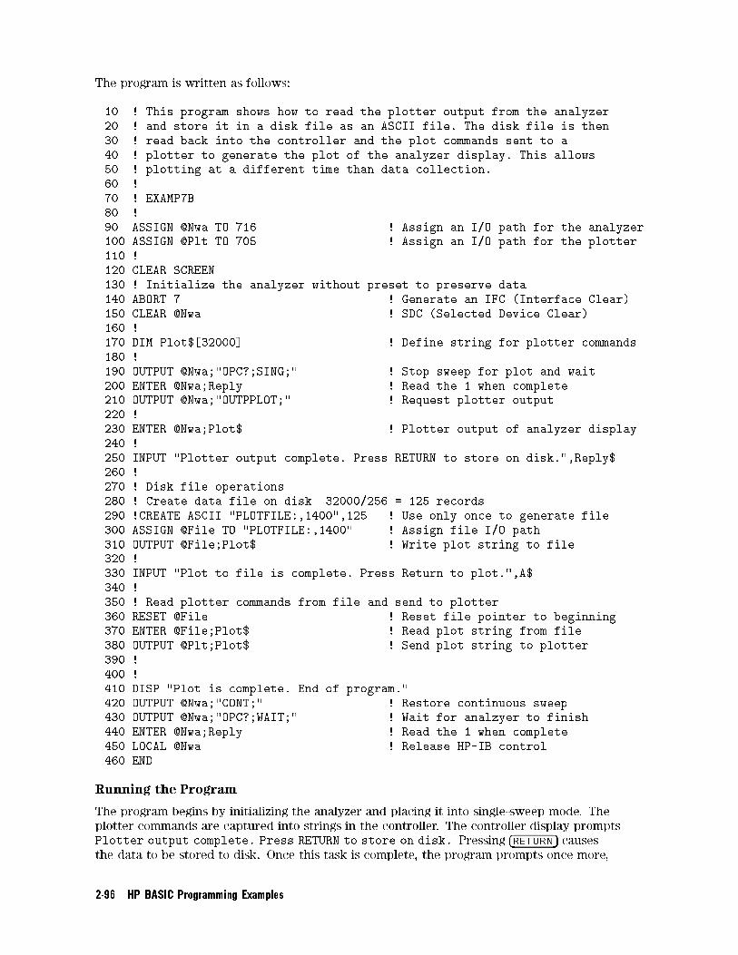
The program is written as follows:
10 ! This program shows how to read the plotter output from the analyzer
20 ! and store it in a disk file as an ASCII file. The disk file is then
30 ! read back into the controller and the plot commands sent to a
40 ! plotter to generate the plot of the analyzer display. This allows
50 ! plotting at a different time than data collection.
60 !
70 ! EXAMP7B
80 !
90 ASSIGN @Nwa TO 716 ! Assign an I/O path for the analyzer
100 ASSIGN @Plt TO 705 ! Assign an I/O path for the plotter
110 !
120 CLEAR SCREEN
130 ! Initialize the analyzer without preset to preserve data
140 ABORT 7 ! Generate an IFC (Interface Clear)
150 CLEAR @Nwa ! SDC (Selected Device Clear)
160 !
170 DIM Plot$[32000] ! Define string for plotter commands
180 !
190 OUTPUT @Nwa;"OPC?;SING;" ! Stop sweep for plot and wait
200 ENTER @Nwa;Reply ! Read the 1 when complete
210 OUTPUT @Nwa;"OUTPPLOT;" ! Request plotter output
220 !
230 ENTER @Nwa;Plot$ ! Plotter output of analyzer display
240 !
250 INPUT "Plotter output complete. Press RETURN to store on disk.",Reply$
260 !
270 ! Disk file operations
280 ! Create data file on disk 32000/256 = 125 records
290 !CREATE ASCII "PLOTFILE:,1400",125 ! Use only once to generate file
300 ASSIGN @File TO "PLOTFILE:,1400" ! Assign file I/O path
310 OUTPUT @File;Plot$ ! Write plot string to file
320 !
330 INPUT "Plot to file is complete. Press Return to plot.",A$
340 !
350 ! Read plotter commands from file and send to plotter
360 RESET @File ! Reset file pointer to beginning
370 ENTER @File;Plot$ ! Read plot string from file
380 OUTPUT @Plt;Plot$ ! Send plot string to plotter
390 !
400 !
410 DISP "Plot is complete. End of program."
420 OUTPUT @Nwa;"CONT;" ! Restore continuous sweep
430 OUTPUT @Nwa;"OPC?;WAIT;" ! Wait for analzyer to finish
440 ENTER @Nwa;Reply ! Read the 1 when complete
450 LOCAL @Nwa ! Release HP-IB control
460 END
Running the Program
The program begins by initializing the analyzer and placing it into single-sweep mode. The
plotter commands are captured into strings in the controller. The controller display prompts
Plotter output complete. Press RETURN to store on disk. Pressing �RETURN� causesthe data to be stored to disk. Once this task is complete, the program prompts once more,
2-96 HP BASIC Programming Examples
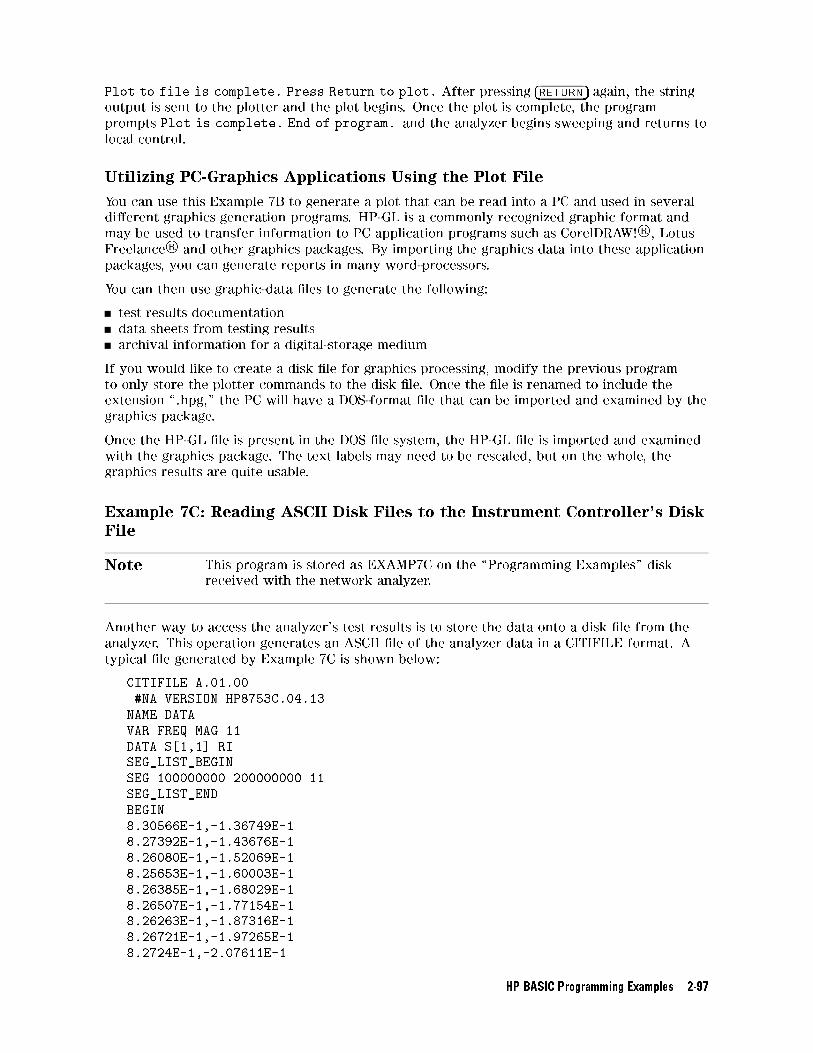
Plot to file is complete. Press Return to plot. After pressing �RETURN� again, the stringoutput is sent to the plotter and the plot begins. Once the plot is complete, the program
prompts Plot is complete. End of program. and the analyzer begins sweeping and returns to
local control.
Utilizing PC-Graphics Applications Using the Plot File
You can use this Example 7B to generate a plot that can be read into a PC and used in several
di�erent graphics generation programs. HP-GL is a commonly recognized graphic format and
may be used to transfer information to PC application programs such as CorelDRAW! R , Lotus
Freelance R and other graphics packages. By importing the graphics data into these application
packages, you can generate reports in many word-processors.
You can then use graphic-data �les to generate the following:
test results documentation
data sheets from testing results
archival information for a digital-storage medium
If you would like to create a disk �le for graphics processing, modify the previous program
to only store the plotter commands to the disk �le. Once the �le is renamed to include the
extension \.hpg," the PC will have a DOS-format �le that can be imported and examined by the
graphics package.
Once the HP-GL �le is present in the DOS �le system, the HP-GL �le is imported and examined
with the graphics package. The text labels may need to be rescaled, but on the whole, the
graphics results are quite usable.
Example 7C: Reading ASCII Disk Files to the Instrument Controller's Disk
File
Note This program is stored as EXAMP7C on the \Programming Examples" disk
received with the network analyzer.
Another way to access the analyzer's test results is to store the data onto a disk �le from the
analyzer. This operation generates an ASCII �le of the analyzer data in a CITIFILE format. A
typical �le generated by Example 7C is shown below:
CITIFILE A.01.00
#NA VERSION HP8753C.04.13
NAME DATA
VAR FREQ MAG 11
DATA S[1,1] RI
SEG_LIST_BEGIN
SEG 100000000 200000000 11
SEG_LIST_END
BEGIN
8.30566E-1,-1.36749E-1
8.27392E-1,-1.43676E-1
8.26080E-1,-1.52069E-1
8.25653E-1,-1.60003E-1
8.26385E-1,-1.68029E-1
8.26507E-1,-1.77154E-1
8.26263E-1,-1.87316E-1
8.26721E-1,-1.97265E-1
8.2724E-1,-2.07611E-1
HP BASIC Programming Examples 2-97
8.28552E-1,-2.19940E-1
8.29620E-1,-2.31109E-1
END
This data �le is stored by the analyzer under remote control or manually from the front panel.
See \Printing, Plotting, or Saving Measurement Results" in the HP 8753D Network Analyzer
User's Guide for more details on manual operation. This program performs the same steps that
are required to manually store a �le from front panel.
This program stores a �le in the same manner as an operator would store a �le on to the
analyzer's internal disk drive from the front panel.
This example explains the process of storing the data from the analyzer to a �le on the internal
disk drive. There is also a program to read the data from the �le into a data array for further
processing or reformatting to another �le type. The internal drive will store in the same
format that is present on the disk. A new disk may be formatted in either LIF or DOS. For the
example, the assumption has been made that the format transformation has already taken
place, and there is a �le that can be read record by record, from which data can be retrieved.
The goal of this example is to recover an array of stimulus frequency along with the trace-data
values. CITIFILES contain the real and imaginary values of each data point. Some further
transformation will be required to obtain magnitude values, for example.
The disk �le contents for this example are shown above. This �le contains more information
than will be used in this example. The �le is accessed and the records read from the �le and
printed on the controller display to observe the actual �le contents. The �le pointer is reset
and the records are then read and interpreted for their data contents.
The �rst six records are skipped for this example. The seventh record contains the
stimulus-frequency values and the number of points in the trace. These values are read
from the record. The frequency increment, or point spacing, is calculated and used later the
frequency-data calculations for a point. Two more records are skipped and the next is the �rst
record representing data values. The data values are read in a loop until the values for the
number of points have been recovered from the �le. The data values are tabulated and printed
out on the controller display.
The following is an outline of the program's processing sequence:
An I/O path is assigned to the analyzer.
The system is initialized.
A string is dimensioned to hold a �le record.
The analyzer operating state is set.
The internal drive is selected for storage (only ASCII data is stored).
A �le name is entered and the data stored into it.
The operator is prompted to move the disk to the controller disk drive.
The disk �le is read and the contents displayed.
The �le pointer is rewound.
The �le contents are converted to trace data.
The frequency and complex-data pair is displayed for each point.
The analyzer is restored to continuous-sweep mode.
The analyzer is returned to local control and the program ends.
2-98 HP BASIC Programming Examples
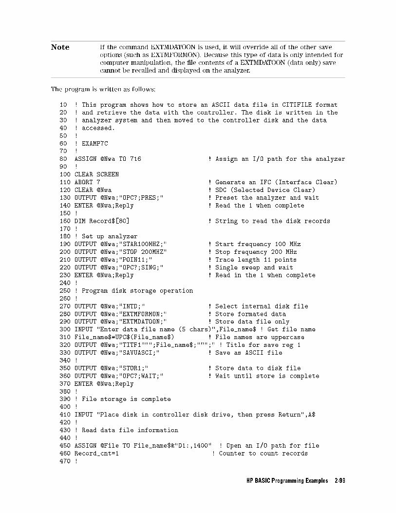
Note If the command EXTMDATOON is used, it will override all of the other save
options (such as EXTMFORMON). Because this type of data is only intended for
computer manipulation, the �le contents of a EXTMDATOON (data only) save
cannot be recalled and displayed on the analyzer.
The program is written as follows:
10 ! This program shows how to store an ASCII data file in CITIFILE format
20 ! and retrieve the data with the controller. The disk is written in the
30 ! analyzer system and then moved to the controller disk and the data
40 ! accessed.
50 !
60 ! EXAMP7C
70 !
80 ASSIGN @Nwa TO 716 ! Assign an I/O path for the analyzer
90 !
100 CLEAR SCREEN
110 ABORT 7 ! Generate an IFC (Interface Clear)
120 CLEAR @Nwa ! SDC (Selected Device Clear)
130 OUTPUT @Nwa;"OPC?;PRES;" ! Preset the analyzer and wait
140 ENTER @Nwa;Reply ! Read the 1 when complete
150 !
160 DIM Record$[80] ! String to read the disk records
170 !
180 ! Set up analyzer
190 OUTPUT @Nwa;"STAR100MHZ;" ! Start frequency 100 MHz
200 OUTPUT @Nwa;"STOP 200MHZ" ! Stop frequency 200 MHz
210 OUTPUT @Nwa;"POIN11;" ! Trace length 11 points
220 OUTPUT @Nwa;"OPC?;SING;" ! Single sweep and wait
230 ENTER @Nwa;Reply ! Read in the 1 when complete
240 !
250 ! Program disk storage operation
260 !
270 OUTPUT @Nwa;"INTD;" ! Select internal disk file
280 OUTPUT @Nwa;"EXTMFORMON;" ! Store formated data
290 OUTPUT @Nwa;"EXTMDATOON;" ! Store data file only
300 INPUT "Enter data file name (5 chars)",File_name$ ! Get file name
310 File_name$=UPC$(File_name$) ! File names are uppercase
320 OUTPUT @Nwa;"TITF1""";File_name$;""";" ! Title for save reg 1
330 OUTPUT @Nwa;"SAVUASCI;" ! Save as ASCII file
340 !
350 OUTPUT @Nwa;"STOR1;" ! Store data to disk file
360 OUTPUT @Nwa;"OPC?;WAIT;" ! Wait until store is complete
370 ENTER @Nwa;Reply
380 !
390 ! File storage is complete
400 !
410 INPUT "Place disk in controller disk drive, then press Return",A$
420 !
430 ! Read data file information
440 !
450 ASSIGN @File TO File_name$&"D1:,1400" ! Open an I/O path for file
460 Record_cnt=1 ! Counter to count records
470 !
HP BASIC Programming Examples 2-99
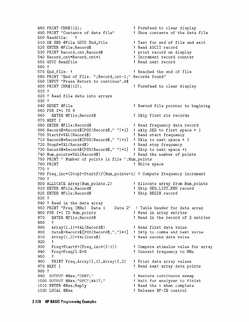
480 PRINT CHR$(12); ! Formfeed to clear display
490 PRINT "Contents of data file" ! Show contents of the data file
500 Readfile: !
510 ON END @File GOTO End_file ! Test for end of file and exit
520 ENTER @File;Record$ ! Read ASCII record
530 PRINT Record_cnt,Record$ ! print record on display
540 Record_cnt=Record_cnt+1 ! Increment record counter
550 GOTO Readfile ! Read next record
560 !
570 End_file: ! ! Reached the end of file
580 PRINT "End of File. ";Record_cnt-1;" Records found"
590 INPUT "Press Return to continue",A$
600 PRINT CHR$(12); ! Formfeed to clear display
610 !
620 ! Read file data into arrays
630 !
640 RESET @File ! Rewind file pointer to begining
650 FOR I=1 TO 6
660 ENTER @File;Record$ ! Skip first six records
670 NEXT I
680 ENTER @File;Record$ ! Read frequency data record
690 Record$=Record$[POS(Record$," ")+1] ! skip SEG to first space + 1
700 Startf=VAL(Record$) ! Read start frequency
710 Record$=Record$[POS(Record$," ")+1] ! Skip to next space + 1
720 Stopf=VAL(Record$) ! Read stop frequency
730 Record$=Record$[POS(Record$," ")+1] ! Skip to next space +1
740 Num_points=VAL(Record$) ! Read the number of points
750 PRINT " Number of points in file ";Num_points
760 PRINT ! White space
770 !
780 Freq_inc=(Stopf-Startf)/(Num_points-1) ! Compute frequency increment
790 !
800 ALLOCATE Array(Num_points,2) ! Allocate array from Num_points
810 ENTER @File;Record$ ! Skip SEG_LIST_END record
820 ENTER @File;Record$ ! Skip BEGIN record
830 !
840 ! Read in the data array
850 PRINT "Freq (MHz) Data 1 Data 2" ! Table header for data array
860 FOR I=1 TO Num_points ! Read in array entries
870 ENTER @File;Record$ ! Read in the record of 2 entries
880 !
890 Array(I,1)=VAL(Record$) ! Read first data value
900 Data$=Record$[POS(Record$,",")+1] ! Skip to comma and next value
910 Array(I,2)=VAL(Data$) ! Read second data value
920 !
930 Freq=Startf+(Freq_inc*(I-1)) ! Compute stimulus value for array
940 Freq=Freq/1.E+6 ! Convert frequency to MHz
950 !
960 PRINT Freq,Array(I,1),Array(I,2) ! Print data array values
970 NEXT I ! Read next array data points
980 !
990 OUTPUT @Nwa;"CONT;" ! Restore continuous sweep
1000 OUTPUT @Nwa;"OPC?;WAIT;" ! Wait for analyzer to finish
1010 ENTER @Nwa;Reply ! Read the 1 when complete
1020 LOCAL @Nwa ! Release HP-IB control
2-100 HP BASIC Programming Examples
1030 END
Running the Program
The analyzer is initialized and the operating range re-de�ned to an 11-point trace from
100 to 200 MHz. This setup gives a restricted range to be evaluated when the ASCII data �le
(CITIFILE) is read in from the controller. The operator is prompted for a 5-character �lename
to use for storing the data. The analyzer is setup for external storage and stores the data �le.
Once the \pass control/storage/return control" operation is complete, the operator is prompted
to place the disk in the controller disk drive and press �RETURN�. The disk is then read and
the records contained in the �le are printed on the controller display. A prompt appears,
Press return to continue, which allows viewing of the �le contents. Once �RETURN� ispressed, the data records are read and decoded and a table of the stimulus frequency and the
data values are printed.
HP BASIC Programming Examples 2-101
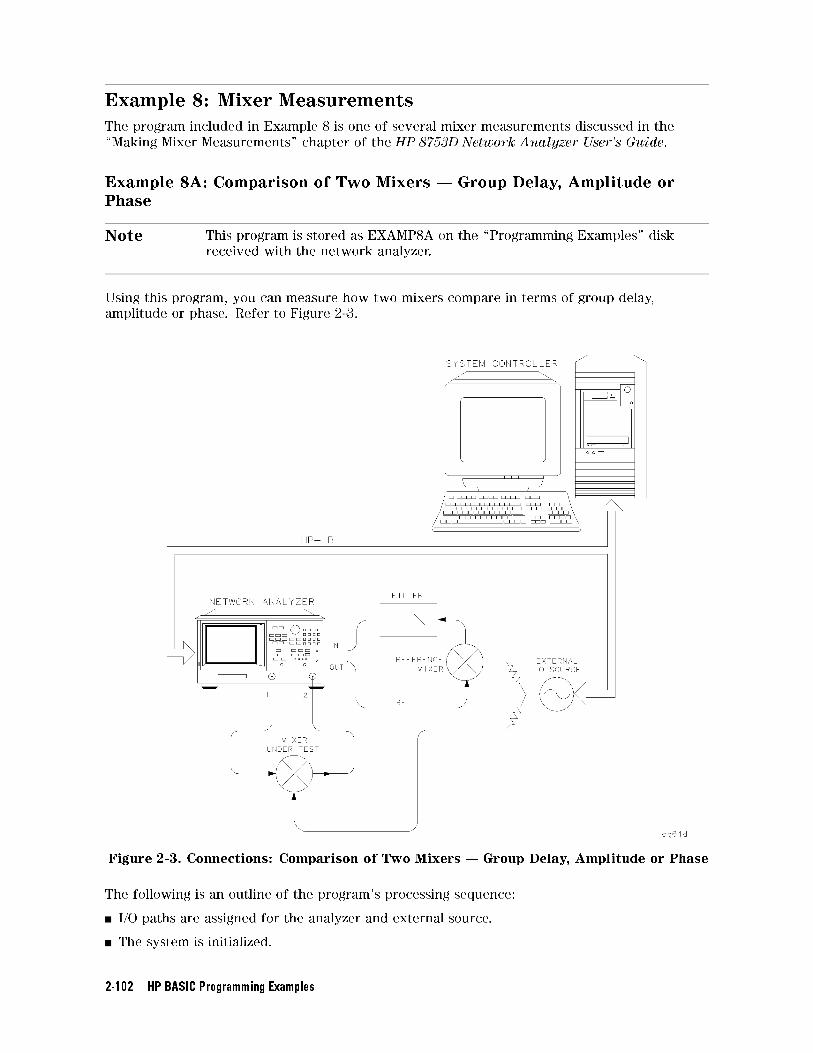
Example 8: Mixer Measurements
The program included in Example 8 is one of several mixer measurements discussed in the
\Making Mixer Measurements" chapter of the HP 8753D Network Analyzer User's Guide.
Example 8A: Comparison of Two Mixers | Group Delay, Amplitude or
Phase
Note This program is stored as EXAMP8A on the \Programming Examples" disk
received with the network analyzer.
Using this program, you can measure how two mixers compare in terms of group delay,
amplitude or phase. Refer to Figure 2-3.
Figure 2-3. Connections: Comparison of Two Mixers | Group Delay, Amplitude or Phase
The following is an outline of the program's processing sequence:
I/O paths are assigned for the analyzer and external source.
The system is initialized.
2-102 HP BASIC Programming Examples
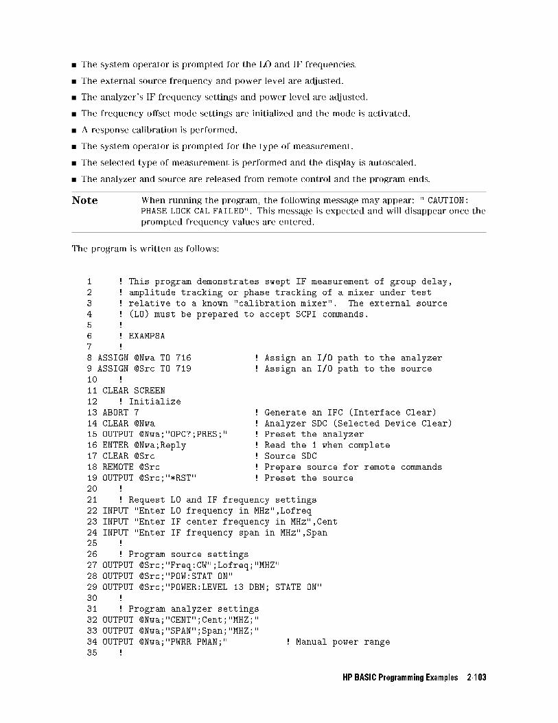
The system operator is prompted for the LO and IF frequencies.
The external source frequency and power level are adjusted.
The analyzer's IF frequency settings and power level are adjusted.
The frequency o�set mode settings are initialized and the mode is activated.
A response calibration is performed.
The system operator is prompted for the type of measurement.
The selected type of measurement is performed and the display is autoscaled.
The analyzer and source are released from remote control and the program ends.
Note When running the program, the following message may appear: " CAUTION:
PHASE LOCK CAL FAILED". This message is expected and will disappear once the
prompted frequency values are entered.
The program is written as follows:
1 ! This program demonstrates swept IF measurement of group delay,
2 ! amplitude tracking or phase tracking of a mixer under test
3 ! relative to a known "calibration mixer". The external source
4 ! (LO) must be prepared to accept SCPI commands.
5 !
6 ! EXAMP8A
7 !
8 ASSIGN @Nwa TO 716 ! Assign an I/O path to the analyzer
9 ASSIGN @Src TO 719 ! Assign an I/O path to the source
10 !
11 CLEAR SCREEN
12 ! Initialize
13 ABORT 7 ! Generate an IFC (Interface Clear)
14 CLEAR @Nwa ! Analyzer SDC (Selected Device Clear)
15 OUTPUT @Nwa;"OPC?;PRES;" ! Preset the analyzer
16 ENTER @Nwa;Reply ! Read the 1 when complete
17 CLEAR @Src ! Source SDC
18 REMOTE @Src ! Prepare source for remote commands
19 OUTPUT @Src;"*RST" ! Preset the source
20 !
21 ! Request LO and IF frequency settings
22 INPUT "Enter LO frequency in MHz",Lofreq
23 INPUT "Enter IF center frequency in MHz",Cent
24 INPUT "Enter IF frequency span in MHz",Span
25 !
26 ! Program source settings
27 OUTPUT @Src;"Freq:CW";Lofreq;"MHZ"
28 OUTPUT @Src;"POW:STAT ON"
29 OUTPUT @Src;"POWER:LEVEL 13 DBM; STATE ON"
30 !
31 ! Program analyzer settings
32 OUTPUT @Nwa;"CENT";Cent;"MHZ;"
33 OUTPUT @Nwa;"SPAN";Span;"MHZ;"
34 OUTPUT @Nwa;"PWRR PMAN;" ! Manual power range
35 !
HP BASIC Programming Examples 2-103
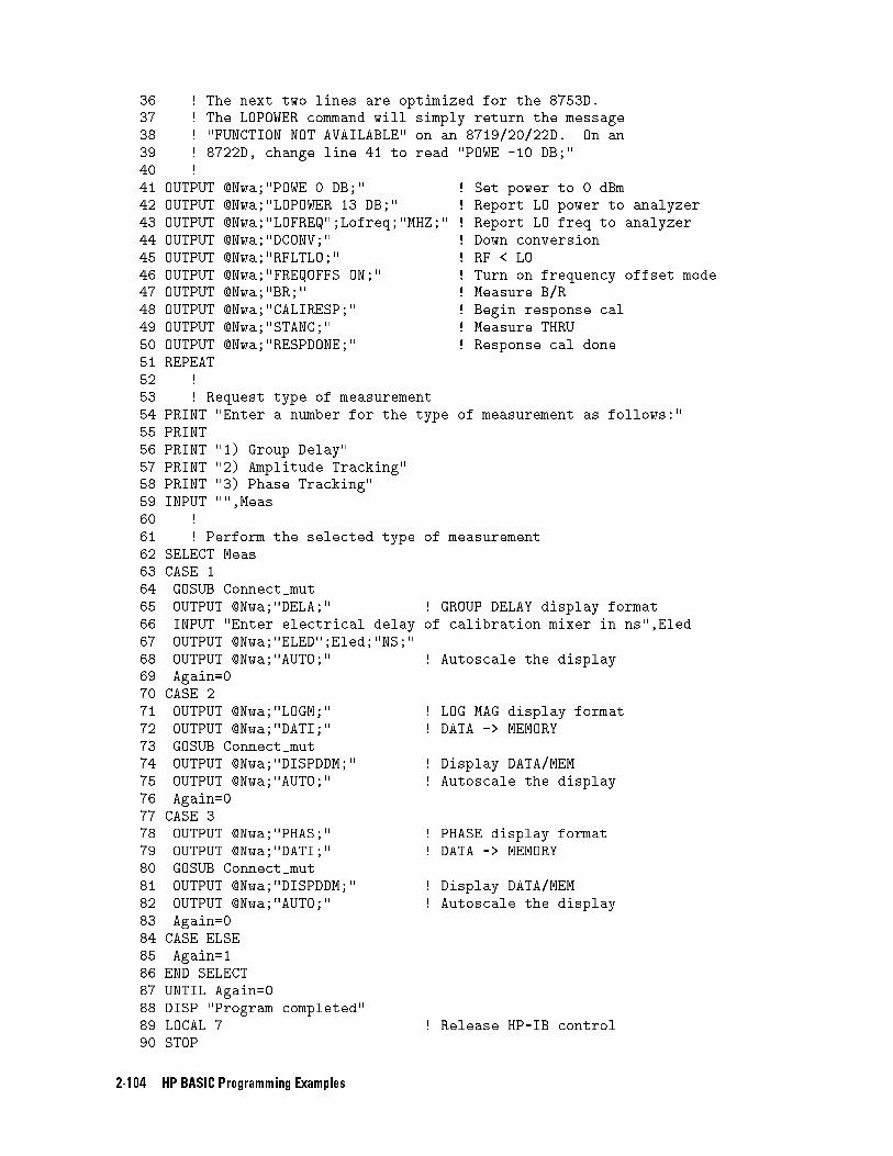
36 ! The next two lines are optimized for the 8753D.
37 ! The LOPOWER command will simply return the message
38 ! "FUNCTION NOT AVAILABLE" on an 8719/20/22D. On an
39 ! 8722D, change line 41 to read "POWE -10 DB;"
40 !
41 OUTPUT @Nwa;"POWE 0 DB;" ! Set power to 0 dBm
42 OUTPUT @Nwa;"LOPOWER 13 DB;" ! Report LO power to analyzer
43 OUTPUT @Nwa;"LOFREQ";Lofreq;"MHZ;" ! Report LO freq to analyzer
44 OUTPUT @Nwa;"DCONV;" ! Down conversion
45 OUTPUT @Nwa;"RFLTLO;" ! RF < LO
46 OUTPUT @Nwa;"FREQOFFS ON;" ! Turn on frequency offset mode
47 OUTPUT @Nwa;"BR;" ! Measure B/R
48 OUTPUT @Nwa;"CALIRESP;" ! Begin response cal
49 OUTPUT @Nwa;"STANC;" ! Measure THRU
50 OUTPUT @Nwa;"RESPDONE;" ! Response cal done
51 REPEAT
52 !
53 ! Request type of measurement
54 PRINT "Enter a number for the type of measurement as follows:"
55 PRINT
56 PRINT "1) Group Delay"
57 PRINT "2) Amplitude Tracking"
58 PRINT "3) Phase Tracking"
59 INPUT "",Meas
60 !
61 ! Perform the selected type of measurement
62 SELECT Meas
63 CASE 1
64 GOSUB Connect_mut
65 OUTPUT @Nwa;"DELA;" ! GROUP DELAY display format
66 INPUT "Enter electrical delay of calibration mixer in ns",Eled
67 OUTPUT @Nwa;"ELED";Eled;"NS;"
68 OUTPUT @Nwa;"AUTO;" ! Autoscale the display
69 Again=0
70 CASE 2
71 OUTPUT @Nwa;"LOGM;" ! LOG MAG display format
72 OUTPUT @Nwa;"DATI;" ! DATA -> MEMORY
73 GOSUB Connect_mut
74 OUTPUT @Nwa;"DISPDDM;" ! Display DATA/MEM
75 OUTPUT @Nwa;"AUTO;" ! Autoscale the display
76 Again=0
77 CASE 3
78 OUTPUT @Nwa;"PHAS;" ! PHASE display format
79 OUTPUT @Nwa;"DATI;" ! DATA -> MEMORY
80 GOSUB Connect_mut
81 OUTPUT @Nwa;"DISPDDM;" ! Display DATA/MEM
82 OUTPUT @Nwa;"AUTO;" ! Autoscale the display
83 Again=0
84 CASE ELSE
85 Again=1
86 END SELECT
87 UNTIL Again=0
88 DISP "Program completed"
89 LOCAL 7 ! Release HP-IB control
90 STOP
2-104 HP BASIC Programming Examples
91 Connect_mut: ! Prompt system operator to replace mixer
92 DISP "Remove calibration mixer, connect MUT, then press Continue"
93 PAUSE
94 RETURN
95 END
Running the Program
The analyzer and source are initialized and the operator is queried for the LO frequency, IF
center frequency and span. The source frequency and power level are set, and the analyzer
frequency settings and power level are adjusted as well. The analyzer frequency o�set mode
settings are adjusted, the frequency o�set mode is turned on, and a response calibration is
performed. The operator is queried for the type of measurement, which is then performed,
and the program ends.
HP BASIC Programming Examples 2-105
Limit Line and Data Point Special Functions
The analyzer has special functions in the area of limit testing and in the detection of min/max
data points within limit segments. The information in this section will teach you how to use
these limit line and data point special functions. The following topics are included:
Overview
Constants Used Throughout This Document
Output Limit Test Pass/Fail Status Per Limit Segment
Output Pass/Fail Status For All Segments
Output Minimum and Maximum Point Per Limit Segment
Output Minimum and Maximum Point For All Segments
Output Data Per Point
Output Data Per Range of Points
Output Limit Pass/Fail by Channel
2-106 HP BASIC Programming Examples
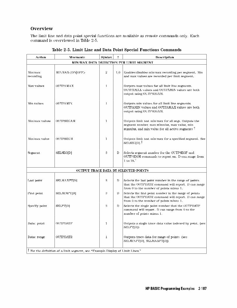
Overview
The limit line and data point special functions are available as remote commands only. Each
command is overviewed in Table 2-5.
Table 2-5. Limit Line and Data Point Special Functions Commands
Action Mnemonic Syntax ? Description
MIN/MAX DATA DETECTION PER LIMIT SEGMENT
Min/max
recording
MINMAX<ONjOFF> 2 1,0 Enables/disables min/max recording per segment. Min
and max values are recorded per limit segment.
Max values OUTPAMAX 1 Outputs max values for all limit line segments.
OUTPAMAX values and OUTPAMIN values are both
output using OUTPSEGAM.
Min values OUTPAMIN 1 Outputs min values for all limit line segments.
OUTPAMIN values and OUTPAMAX values are both
output using OUTPSEGAM.
Min/max values OUTPSEGAM 1 Outputs limit test min/max for all segs. Outputs the
segment number, max stimulus, max value, min
stimulus, and min value for all active segments.y
Min/max value OUTPSEGM 1 Outputs limit test min/max for a speci�ed segment. See
SELSEG[D].y
Segment SELSEG[D] 3 D Selects segment number for the OUTPSEGF and
OUTPSEGM commands to report on. D can range from
1 to 18.y
OUTPUT TRACE DATA BY SELECTED POINTS
Last point SELMAXPT[D] 3 D Selects the last point number in the range of points
that the OUTPDATR command will report. D can range
from 0 to the number of points minus 1.
First point SELMINPT[D] 3 D Selects the �rst point number in the range of points
that the OUTPDATR command will report. D can range
from 0 to the number of points minus 1.
Specify point SELPT[D] 3 D Selects the single point number that the OUTPDATP
command will report. D can range from 0 to the
number of points minus 1.
Data: point OUTPDATP 1 Outputs a single trace data value indexed by point. (see
SELPT[D])
Data: range OUTPDATR 1 Outputs trace data for range of points. (see
SELMINPT[D], SELMAXPT[D])
y For the de�nition of a limit segment, see \Example Display of Limit Lines."
HP BASIC Programming Examples 2-107
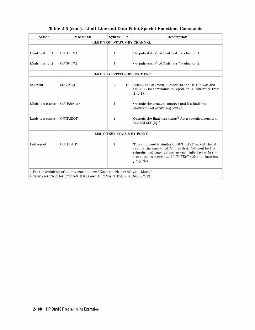
Table 2-5 (cont). Limit Line and Data Point Special Functions Commands
Action Mnemonic Syntax ? Description
LIMIT TEST STATUS BY CHANNEL
Limit test: ch1 OUTPLIM1 1 Outputs statusx of limit test for channel 1.
Limit test: ch2 OUTPLIM2 1 Outputs statusx of limit test for channel 2.
LIMIT TEST STATUS BY SEGMENT
Segment SELSEG[D] 3 D Selects the segment number for the OUTPSEGF and
OUTPSEGM commands to report on. D can range from
1 to 18.y
Limit test status OUTPSEGAF 1 Outputs the segment number and it's limit test
statusxfor all active segments.y
Limit test status OUTPSEGF 1 Outputs the limit test statusx for a speci�ed segment.
See SELSEG[D].y
LIMIT TEST STATUS BY POINT
Fail report OUTPFAIP 1 This command is similar to OUTPLIMF except that it
reports the number of failures �rst, followed by the
stimulus and trace values for each failed point in the
test (note: use command LIMITEST<ON> to function
properly).
y For the de�nition of a limit segment, see \Example Display of Limit Lines."x Values returned for limit test status are: 1 (PASS), 0 (FAIL), -1 (NO LIMIT)
2-108 HP BASIC Programming Examples
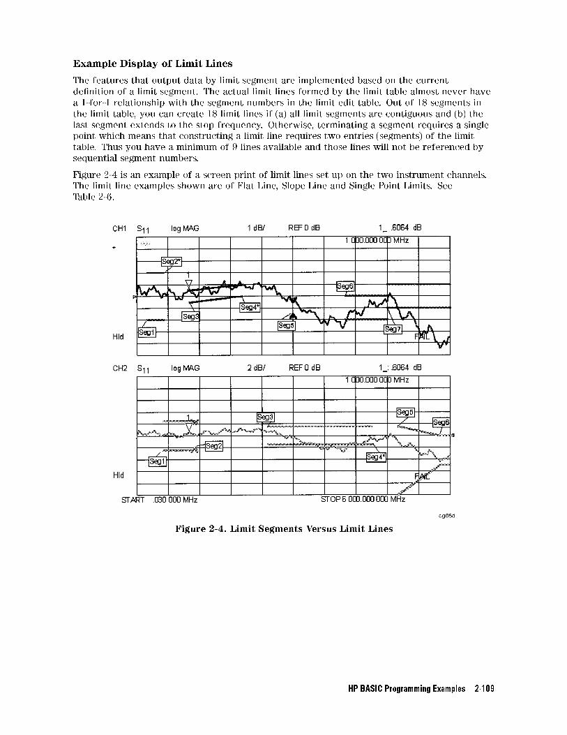
Example Display of Limit Lines
The features that output data by limit segment are implemented based on the current
de�nition of a limit segment. The actual limit lines formed by the limit table almost never have
a 1-for-1 relationship with the segment numbers in the limit edit table. Out of 18 segments in
the limit table, you can create 18 limit lines if (a) all limit segments are contiguous and (b) the
last segment extends to the stop frequency. Otherwise, terminating a segment requires a single
point which means that constructing a limit line requires two entries (segments) of the limit
table. Thus you have a minimum of 9 lines available and those lines will not be referenced by
sequential segment numbers.
Figure 2-4 is an example of a screen print of limit lines set up on the two instrument channels.
The limit line examples shown are of Flat Line, Slope Line and Single Point Limits. See
Table 2-6.
Figure 2-4. Limit Segments Versus Limit Lines
HP BASIC Programming Examples 2-109
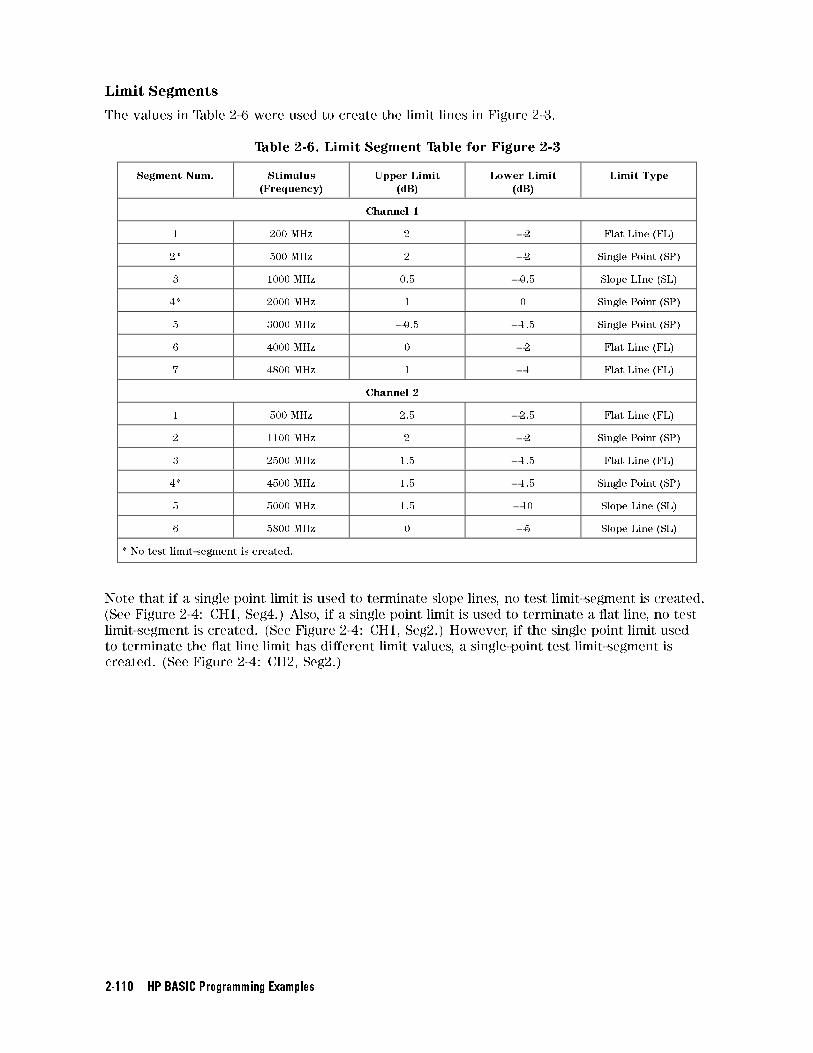
Limit Segments
The values in Table 2-6 were used to create the limit lines in Figure 2-3.
Table 2-6. Limit Segment Table for Figure 2-3
Segment Num. Stimulus
(Frequency)
Upper Limit
(dB)
Lower Limit
(dB)
Limit Type
Channel 1
1 200 MHz 2 �2 Flat Line (FL)
2* 500 MHz 2 �2 Single Point (SP)
3 1000 MHz 0.5 �0.5 Slope LIne (SL)
4* 2000 MHz 1 0 Single Point (SP)
5 3000 MHz �0.5 �1.5 Single Point (SP)
6 4000 MHz 0 �2 Flat Line (FL)
7 4800 MHz 1 �1 Flat Line (FL)
Channel 2
1 500 MHz 2.5 �2.5 Flat Line (FL)
2 1100 MHz 2 �2 Single Point (SP)
3 2500 MHz 1.5 �1.5 Flat Line (FL)
4* 4500 MHz 1.5 �1.5 Single Point (SP)
5 5000 MHz 1.5 �10 Slope Line (SL)
6 5800 MHz 0 �5 Slope Line (SL)
* No test limit-segment is created.
Note that if a single point limit is used to terminate slope lines, no test limit-segment is created.
(See Figure 2-4: CH1, Seg4.) Also, if a single point limit is used to terminate a at line, no test
limit-segment is created. (See Figure 2-4: CH1, Seg2.) However, if the single point limit used
to terminate the at line limit has di�erent limit values, a single-point test limit-segment is
created. (See Figure 2-4: CH2, Seg2.)
2-110 HP BASIC Programming Examples
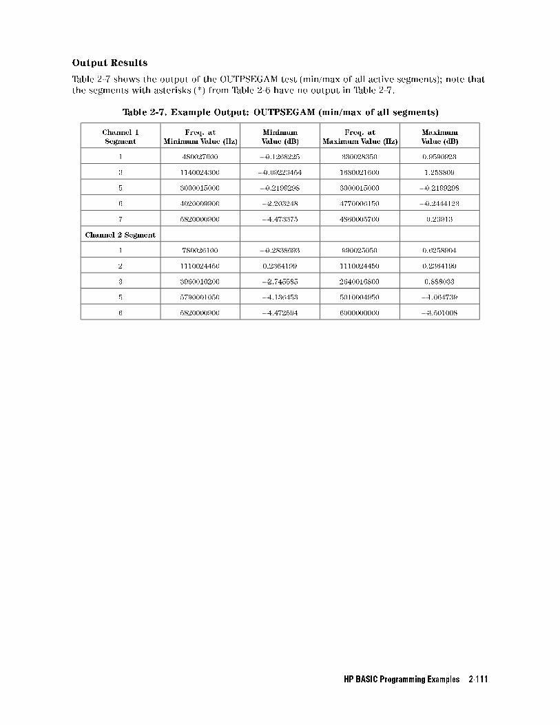
Output Results
Table 2-7 shows the output of the OUTPSEGAM test (min/max of all active segments); note that
the segments with asterisks (*) from Table 2-6 have no output in Table 2-7.
Table 2-7. Example Output: OUTPSEGAM (min/max of all segments)
Channel 1
Segment
Freq. at
Minimum Value (Hz)
Minimum
Value (dB)
Freq. at
Maximum Value (Hz)
Maximum
Value (dB)
1 480027600 �0.1268225 330028350 0.9590923
3 1140024300 �0.09223454 1680021600 1.258809
5 3000015000 �0.2199298 3000015000 �0.2199298
6 4020009900 �2.203248 4770006150 �0.2444123
7 5820000900 �4.473375 4860005700 0.23913
Channel 2 Segment
1 780026100 �0.2838693 990025050 0.6258904
2 1110024450 0.2364199 1110024450 0.2364199
3 3960010200 �2.745585 2640016800 0.888033
5 5790001050 �4.136453 5010004950 �1.064739
6 5820000900 �4.472594 6000000000 �3.501008
HP BASIC Programming Examples 2-111
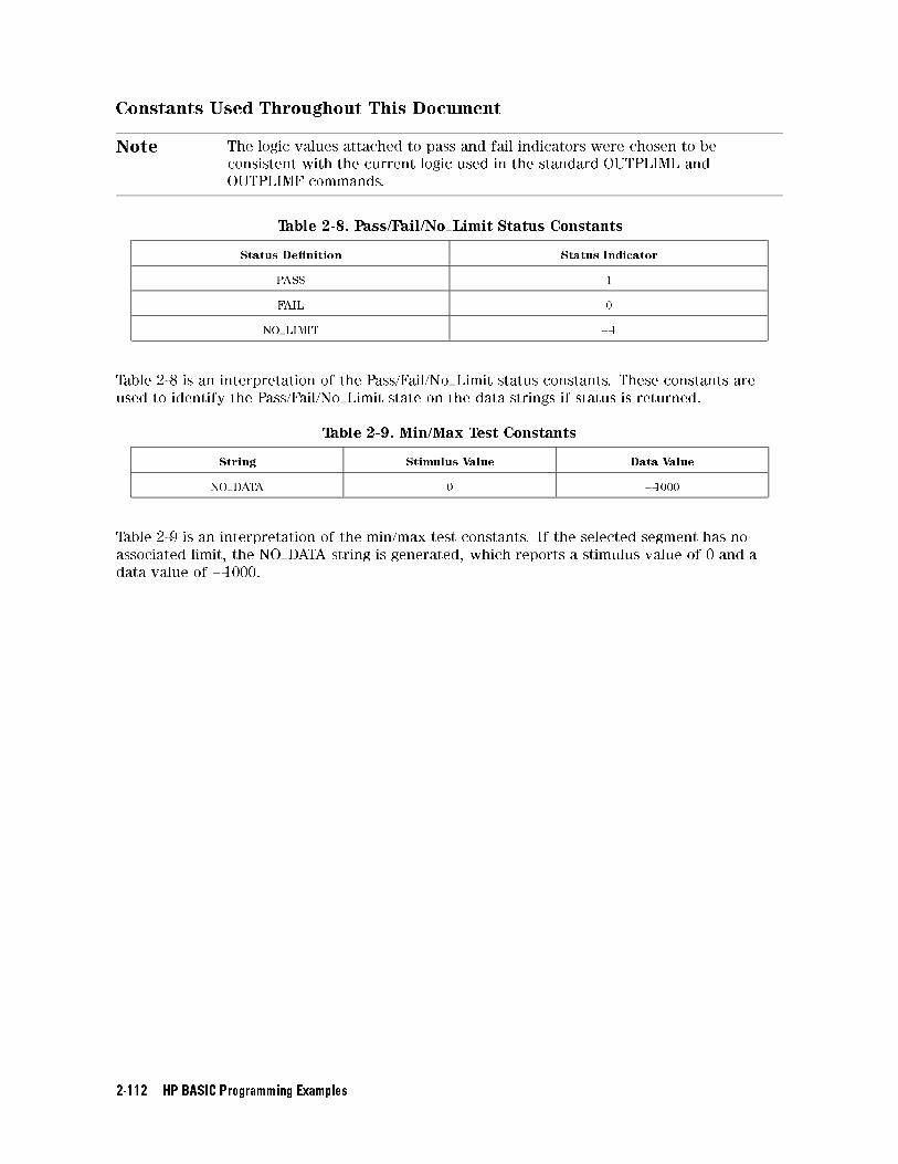
Constants Used Throughout This Document
Note The logic values attached to pass and fail indicators were chosen to be
consistent with the current logic used in the standard OUTPLIML and
OUTPLIMF commands.
Table 2-8. Pass/Fail/No Limit Status Constants
Status De�nition Status Indicator
PASS 1
FAIL 0
NO LIMIT �1
Table 2-8 is an interpretation of the Pass/Fail/No Limit status constants. These constants are
used to identify the Pass/Fail/No Limit state on the data strings if status is returned.
Table 2-9. Min/Max Test Constants
String Stimulus Value Data Value
NO DATA 0 �1000
Table 2-9 is an interpretation of the min/max test constants. If the selected segment has no
associated limit, the NO DATA string is generated, which reports a stimulus value of 0 and a
data value of �1000.
2-112 HP BASIC Programming Examples
Output Limit Test Pass/Fail Status Per Limit Segment
Two commands allow you to query the pass/fail test status on a limit segment basis: (See
previous discussion about segment numbers.)
SELSEG[D] will select the segment.
OUTPSEGF will return the status of the limit test for that segment: 1 (PASS), 0 (FAIL) or �1(NO LIMIT) if no limit exists for the selected segment number. Due to the non-sequential
numbering of actual limit line segments on the screen, some segment numbers will have no
associated limits and will thus return NO LIMIT (�1).
Under the following conditions, OUTPSEGF will issue the following errors:
If the limit testing is OFF: \30: Requested Data Not Currently Available." To clear the
error message, turn the limit test ON.
If the limit table is empty: \204: Limit Table Empty" (this is a new message). To clear the
error message, enter a limit table.
In both cases, the error is issued and the command responds with �1 (NO LIMIT).
The argument for SELSEG[D] is limited by the maximum number of segments allowed in the
limit table, which is currently 18. The minimum value for the argument is 1. If the user inputs
a number that is outside this range, the active entry limits are invoked, causing the analyzer to
return the status for limit 18.
Example:
Sending SELSEG3 and OUTPSEGF may return the following:
1 (segment number 3 passed)
Note The output is ASCII. Currently, the formatting for integer numbers appears to
append a trailing space.
HP BASIC Programming Examples 2-113
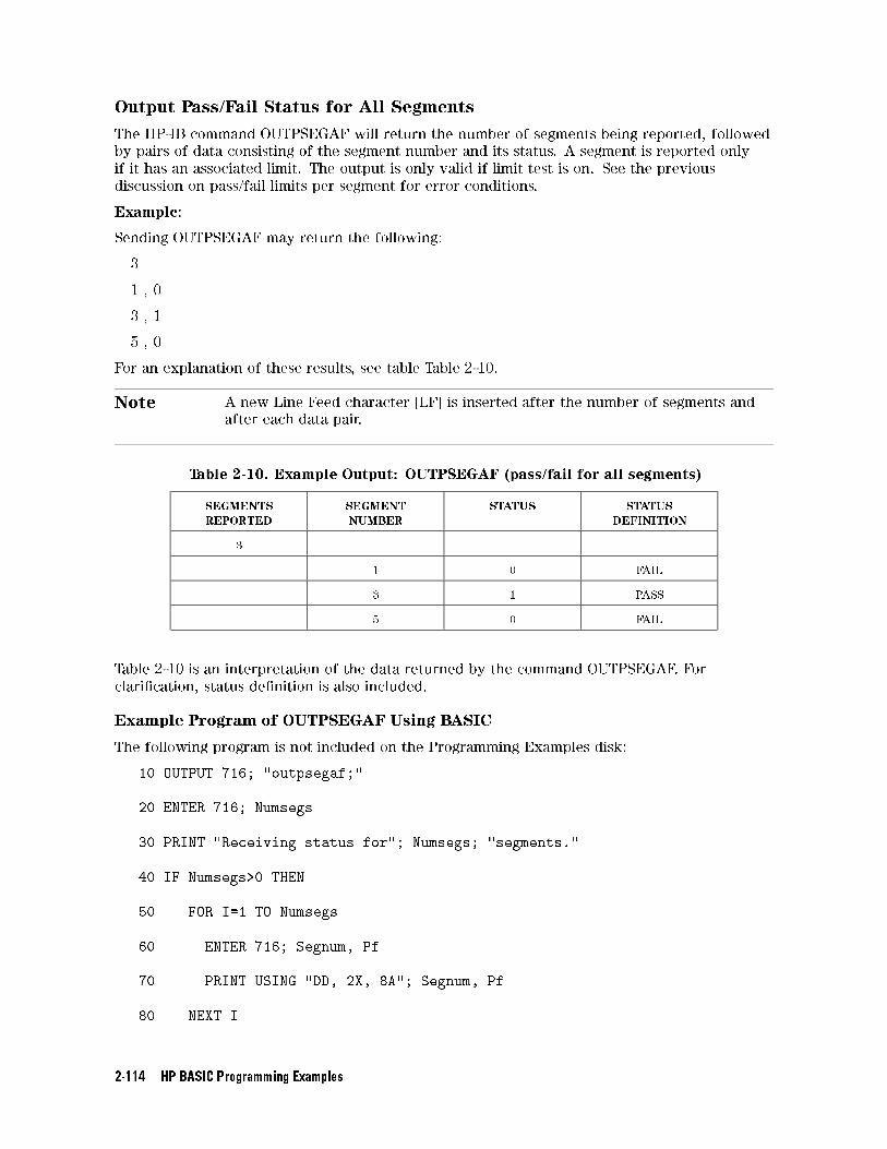
Output Pass/Fail Status for All Segments
The HP-IB command OUTPSEGAF will return the number of segments being reported, followed
by pairs of data consisting of the segment number and its status. A segment is reported only
if it has an associated limit. The output is only valid if limit test is on. See the previous
discussion on pass/fail limits per segment for error conditions.
Example:
Sending OUTPSEGAF may return the following:
3
1 , 0
3 , 1
5 , 0
For an explanation of these results, see table Table 2-10.
Note A new Line Feed character [LF] is inserted after the number of segments and
after each data pair.
Table 2-10. Example Output: OUTPSEGAF (pass/fail for all segments)
SEGMENTS
REPORTED
SEGMENT
NUMBER
STATUS STATUS
DEFINITION
3
1 0 FAIL
3 1 PASS
5 0 FAIL
Table 2-10 is an interpretation of the data returned by the command OUTPSEGAF. For
clari�cation, status de�nition is also included.
Example Program of OUTPSEGAF Using BASIC
The following program is not included on the Programming Examples disk:
10 OUTPUT 716; "outpsegaf;"
20 ENTER 716; Numsegs
30 PRINT "Receiving status for"; Numsegs; "segments."
40 IF Numsegs>0 THEN
50 FOR I=1 TO Numsegs
60 ENTER 716; Segnum, Pf
70 PRINT USING "DD, 2X, 8A"; Segnum, Pf
80 NEXT I
2-114 HP BASIC Programming Examples

The example program shows how the OUTPSEGAF command can be used to request the
number of active segments and their status. Notice that each segment result must use a new
enter command as a line feed terminates each segment data result.
HP BASIC Programming Examples 2-115

Output Minimum and Maximum Point Per Limit Segment
The command \MINMAX"[ONjOFF] toggles a feature which records the minimum and maximum
data points in all active limit segments. Note that limit testing need not be turned on.
The command OUTPSEGM will report the min/max data for the segment previously selected
by SELSEG[N]. The data is returned in a comma delimited string with the segment number,
minimum point stimulus, minimum trace value, maximum point stimulus and maximum trace
value.
Under the following conditions, OUTPSEGM will issue the following errors:
If the min/max testing is OFF: \30: Requested Data Not Currently Available." To clear the
error message, turn the min/max testing ON.
If the limit table is empty: \204: Limit Table Empty" ( this is a new message). To clear the
error message, enter a new limit table.
When the above error conditions occur, there is no data to report, thus no output is
generated.
If the selected segment has no associated limit, the NO DATA string is generated, which
reports a stimulus value of 0 and a data value of �1000.
Example:
Sending SELSEG3 and OUTPSEGM may return the following:
3, 1.900000000E+09, �9.900000E�01, 2.123456789E+09, 2.123456E+00
For an explanation of these results, see Table 2-11.
Table 2-11. Example Output: OUTPSEGM (min/max per segment)
SEGMENT MIN PT STIMULUS
(FREQUENCY)
MIN PT VALUE
(dB)
MAX PT STIMULUS
(FREQUENCY)
MAX PT VALUE
(dB)
3 1.9 GHz �.99 2.12 GHz 2.12
Table 2-11 is an interpretation of the min/max data returned using the SELSEG[N] and
OUTPSEGM commands.
Note A new Line Feed character [LF] is inserted after the segment number and after
each data pair.
2-116 HP BASIC Programming Examples
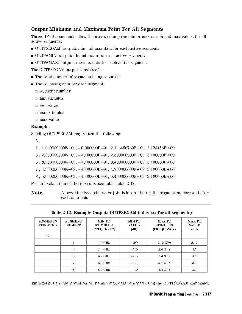
Output Minimum and Maximum Point For All Segments
Three HP-IB commands allow the user to dump the min-or-max or min-and-max values for all
active segments:
OUTPSEGAM: outputs min and max data for each active segment.
OUTPAMIN: outputs the min data for each active segment.
OUTPAMAX: outputs the max data for each active segment.
The OUTPSEGAM output consists of :
The total number of segments being reported.
The following data for each segment:
segment number
min stimulus
min value
max stimulus
max value
Example:
Sending OUTPSEGAM may return the following:
5 ,
1 , 1.900000000E+09, �9.900000E�01, 2.123456789E+09, 2.123456E+00
3 , 2.300000000E+09, �10.00000E�01, 2.600000000E+09, 3.100000E+00
5 , 3.200000000E+09, �10.00000E�01, 3.400000000E+09, 3.100000E+00
7 , 4.300000000E+09, �10.00000E�01, 4.700000000E+09, 3.100000E+00
8 , 5.000000000E+09, �10.00000E�01, 5.400000000E+09, 3.100000E+00
For an explanation of these results, see table Table 2-12.
Note A new Line Feed character [LF] is inserted after the segment number and after
each data pair.
Table 2-12. Example Output: OUTPSEGAM (min/max for all segments)
SEGMENTS
REPORTED
SEGMENT
NUMBER
MIN PT
STIMULUS
(FREQUENCY)
MIN PT
VALUE
(dB)
MAX PT
STIMULUS
(FREQUENCY)
MAX PT
VALUE
(dB)
5
1 1.9 GHz �.99 2.12 GHz 2.12
3 2.3 GHz �1.0 2.6 GHz 3.1
5 3.2 GHz �1.0 3.4 GHz 3.1
7 4.3 GHz �1.0 4.7 GHz 3.1
8 5.0 GHz �1.0 5.4 GHz 3.1
Table 2-12 is an interpretation of the min/max data returned using the OUTPSEGAM command.
HP BASIC Programming Examples 2-117
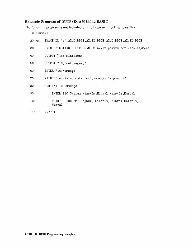
Example Program of OUTPSEGAM Using BASIC
The following program is not included on the Programming Examples disk:
10 Minmax: !
20 Mm: IMAGE DD,":",2X,D.DDDE,2X,SD.DDDE,2X,D.DDDE,2X,SD.DDDE
30 PRINT "TESTING: OUTPSEGAM: min/max points for each segment"
40 OUTPUT 716;"minmaxon;"
50 OUTPUT 716;"outpsegam;"
60 ENTER 716;Numsegs
70 PRINT "receiving data for";Numsegs;"segments"
80 FOR I=1 TO Numsegs
90 ENTER 716;Segnum,Minstim,Minval,Maxstim,Maxval
100 PRINT USING Mm; Segnum, Minstim, Minval,Maxstim,
Maxval
110 NEXT I
2-118 HP BASIC Programming Examples
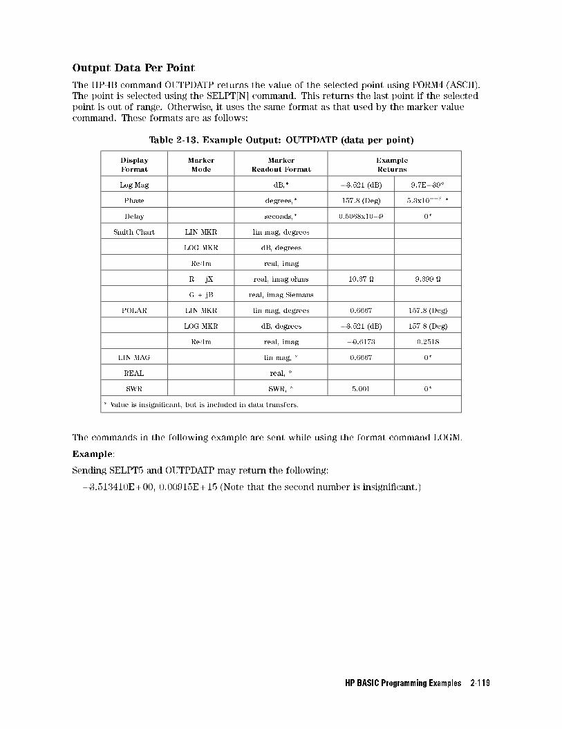
Output Data Per Point
The HP-IB command OUTPDATP returns the value of the selected point using FORM4 (ASCII).
The point is selected using the SELPT[N] command. This returns the last point if the selected
point is out of range. Otherwise, it uses the same format as that used by the marker value
command. These formats are as follows:
Table 2-13. Example Output: OUTPDATP (data per point)
Display
Format
Marker
Mode
Marker
Readout Format
Example
Returns
Log Mag dB,* �3.521 (dB) 9.7E�39*
Phase degrees,* 157.8 (Deg) 5.3x10�15 *
Delay seconds,* 0.5068x10�9 0*
Smith Chart LIN MKR lin mag, degrees
LOG MKR dB, degrees
Re/Im real, imag
R + jX real, imag ohms 10.37 9.399
G + jB real, imag Siemans
POLAR LIN MKR lin mag, degrees 0.6667 157.8 (Deg)
LOG MKR dB, degrees �3.521 (dB) 157.8 (Deg)
Re/Im real, imag �0.6173 0.2518
LIN MAG lin mag, * 0.6667 0*
REAL real, *
SWR SWR, * 5.001 0*
* Value is insigni�cant, but is included in data transfers.
The commands in the following example are sent while using the format command LOGM.
Example:
Sending SELPT5 and OUTPDATP may return the following:
�3.513410E+00, 0.00915E+15 (Note that the second number is insigni�cant.)
HP BASIC Programming Examples 2-119
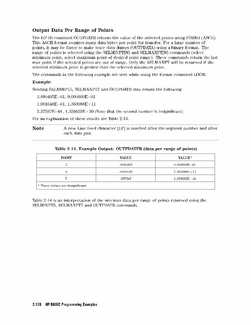
Output Data Per Range of Points
The HP-IB command OUTPDATR returns the value of the selected points using FORM4 (ASCII).
This ASCII format requires many data bytes per point for transfer. For a large number of
points, it may be faster to make trace data dumps (OUTPDATA) using a binary format. The
range of points is selected using the SELMINPT[N] and SELMAXPT[N] commands (select
minimum point, select maximum point of desired point range). These commands return the last
max point if the selected points are out of range. Only the SELMAXPT will be returned if the
selected minimum point is greater than the selected maximum point.
The commands in the following example are sent while using the format command LOGM.
Example:
Sending SELMINPT5, SELMAXPT7 and OUTPDATR may return the following:
3.880465E�01, 0.000039E�01
1.901648E�01, 1.363988E+11
5.57587E�01, 1.258655E+30 (Note that the second number is insigni�cant)
For an explanation of these results see Table 2-14.
Note A new Line Feed character [LF] is inserted after the segment number and after
each data pair.
Table 2-14. Example Output: OUTPDATPR (data per range of points)
POINT VALUE VALUE*
5 .3880465 0.000039E�01
6 .1901648 1.363988E+11
7 .557587 1.258655E+30
* These values are insigni�cant.
Table 2-14 is an interpretation of the min/max data per range of points returned using the
SELMINPT5, SELMAXPT7 and OUTPDATR commands.
2-120 HP BASIC Programming Examples
Output Limit Pass/Fail by Channel
The HP-IB commands OUTPLIM1 and OUTPLIM2 output the status of the limit test for channel
1 and channel 2, respectively.
These commands return the values 1 (PASS), 0 (FAIL), or �1 (NO LIMIT) if limit testing is
disabled. Currently, the results of limit testing can be retrieved by reading a bit in the status
register.
Example:
Sending OUTPLIM1 or OUTPLIM2 (channel 1 or channel 2) may return the following:
1 (PASS), 0 (FAIL), or if limit test not enabled then �1 (NO LIMIT).
HP BASIC Programming Examples 2-121

Index
Special characters
$, 1-33
A
AB, 1-44, 1-64
abort message (IFC), 1-12
abort sequence, 2-8
ADAP1[D], 1-33, 1-64
adapter
coax, 1-64
waveguide, 1-64
adapter delay, 1-64
adapter removal
coax, 1-64
compute new cal set, 1-79
recall cal set, 1-66
waveguide, 1-64
adapter removal calibration, 2-27
additional information, 2-1
BASIC 6.2, 2-1
ADDRCONT[D], 1-44, 1-64
ADDRDISC[D], 1-44, 1-64
address
controller, 1-64
disk drive, 1-64
LO Source, 1-64
peripheral, 1-64
plotter, 1-64
power meter, 1-64
printer, 1-64
address capability, 1-8
addresses for HP-IB, 1-12
ADDRLSRC[D], 1-54, 1-64
ADDRPERI[D], 1-52, 1-64
ADDRPLOT[D], 1-44, 1-64
ADDRPOWM[D], 1-44, 1-64
ADDRPRIN[D], 1-44, 1-64
adjust brightness, 1-66
adjust color, 1-67
adjust tint, 1-95
ADPTCOAX, 1-64
ADPTCOAX , 1-33
ADPTWAVE, 1-33, 1-64
AH1 (full-acceptor handshake), 1-9
ALC, 1-64
ALC control, 1-64
ALTAB, 1-33, 1-64
alternate inputs, 1-64
amplitude and phase tracking, 2-102
amplitude tracking, 2-102
ANAB<ONjOFF>, 1-54, 1-64ANAI[D], 1-44, 1-64
analog bus, 1-64
analog input, 1-64
analyzer array-data formats, 1-18
analyzer bus mode, 1-11
analyzer command syntax, 1-3
analyzer control of peripherals, 1-11
analyzer data reading, 1-15
analyzer-debug mode, 2-14
analyzer features helpful in developing
programs, 2-14
analyzer identi�cation, 1-15
analyzer operating modes, 2-4
pass-control mode, 2-4, 2-90
system-control mode, 2-4
talker/listener, 2-4
analyzer operation, 1-14
analyzer single bus concept, 1-10
analyzer status reporting structure, 1-25
appendage in syntax, 1-4
AR, 1-44, 1-64
array-data formats, 1-17, 2-47
FORM 1, 2-47
FORM 2, 2-47
FORM 3, 2-47
FORM 4, 2-45, 2-47
FORM 5, 2-47
arrays of data, 1-21
arrays related to frequency, 1-20
ASCII
save format, 1-89
ASCII disk �les, 2-97
reading, 2-97
ASEG, 1-47, 1-48, 1-64
assert sequence, 1-64
ASSS, 1-52, 1-64
ATN (attention) control line, 1-7
attention (ATN) control line, 1-7
attenuator o�sets, 2-36
ATTP1, 1-64
ATTP1[D], 1-46
Index-1
ATTP2, 1-64
ATTP2[D], 1-46
AUTO, 1-51, 1-64
auto feed
plotter, 1-84
printer, 1-86
auto scale, 1-64
averaging, 1-64
restart, 1-64
averaging factor, 1-64
AVERFACT[D], 1-33, 1-64
AVERO<ONjOFF>, 1-33, 1-64AVERREST, 1-33, 1-64
B
BACI[D], 1-43, 1-64
background intensity, 1-64
BANDPASS, 1-56, 1-64
basic talker (T6), 1-9
baud rate
plotter, 1-85
printer, 1-86
beep
emit, 1-71
BEEPDONE<ONjOFF>, 1-43, 1-64beeper on done, 1-64
beeper on warning, 1-65
BEEPFAIL<ONjOFF>, 1-55, 1-64BEEPWARN<ONjOFF>, 1-43, 1-65begin cal sequence, 1-65
bi-directional lines, 1-7
binary
save format, 1-89
BLAD<ONjOFF>, 1-43, 1-65blank display, 1-65
BR, 1-44, 1-65
bus device modes, 1-10
bus structure, 1-6, 1-7
C
C0[D], 1-35, 1-65
C10 (pass control capabilities), 1-9
C1,C2,C3 (system controller capabilities),
1-9
C1[D], 1-35, 1-65
C2[D], 1-35, 1-65
C3[D], 1-35, 1-65
CAL1, 1-58, 1-65
CALFCALF[D], 1-40, 1-65
CALFFREQ[D], 1-40, 1-65
CALFSENA, 1-40, 1-65
CALFSENB, 1-40, 1-65
calibrating the test setup, 2-11
calibration
adapter removal , 2-27
power meter, 1-87
simulated, 2-29
using raw data, 2-29
calibration arrays, 1-29
calibration/classes relationship, 1-28
calibration coe�cients, 1-21, 1-24, 1-29
calibration command sequence, 1-28
calibration data
inputting, 2-70
outputting, 2-70
reading, 2-70
calibration kit, 2-2
calibration kits, 1-65, 2-19
calibration kit string and learn string, 1-24
calibration type o�, 1-66
CALIFUL2, 1-33, 1-65
CALIONE2, 1-33, 1-65
CALIRAI, 1-33, 1-65
CALIRESP, 1-33, 1-65
CALIS111, 1-33, 1-65
CALIS221, 1-33, 1-65
CALITRL2, 1-33, 1-65
CALK24MM, 1-35, 1-65
CALK292MM, 1-35, 1-65
CALK292S, 1-35, 1-65
CALK35MC, 1-35, 1-65
CALK35MD, 1-35, 1-65
CALK35MM, 1-35, 1-65
CALK7MM, 1-35, 1-65
cal kit done, 1-74
CALKN50, 1-35, 1-65
CALKN75, 1-35, 1-66
CALKTRLK, 1-35, 1-66
CALKUSED, 1-35, 1-66
CALN, 1-33, 1-66
CALPOW, 1-66
cal power
set port 1, 1-87
cal sensor table
edit, 1-65
cal sequence
begin, 1-65
resume, 1-88
CALSPORT1, 1-33, 1-66
CALSPORT2, 1-33, 1-66
CALZLINE, 1-39, 1-66
CALZSYST[D], 1-39, 1-66
CBRI[D], 1-43, 1-66
CENT[D], 1-48, 1-54, 1-66
center, 1-66
chain for data processing, 1-21
CHAN1, 1-40, 1-66
CHAN2, 1-40, 1-66
channels
coupled, 1-68
Index-2
characters that are valid, 1-4
CHOPAB, 1-33, 1-66
citi�le
save format, 1-89
CLAD, 1-39, 1-66
CLASS11A, 1-35, 1-66
CLASS11B, 1-35, 1-66
CLASS11C, 1-35, 1-66
CLASS22A, 1-35, 1-66
CLASS22B, 1-35, 1-66
CLASS22C, 1-35, 1-66
class done, 1-66
CLEABIT[D], 1-52, 1-67
CLEA<I>, 1-50, 1-66
CLEAL, 1-55, 1-66
CLEARALL, 1-50, 1-66
clear device, 1-12
CLEAREG<I>, 1-50, 1-67
clearing any messages waiting to be output,
2-8
clearing syntax errors, 2-8
clearing the input-command bu�er, 2-8
clear list, 1-67
clear register, 1-66
clear sequence, 1-67, 2-8
CLEASEQ<I>, 1-51, 1-67
CLEL, 1-40, 1-47, 1-67
CLES, 1-63, 1-67
CLS, 1-63, 1-67
COAD, 1-51, 1-67
COAX, 1-36, 1-67
coax adapter, 1-64
code naming conventions, 1-3
code syntax structure, 1-4
collect raw data, 1-94
COLOCH1D, 1-67
COLOCH1D[D], 1-43
COLOCH1M, 1-67
COLOCH1M[D], 1-43
COLOCH2D, 1-67
COLOCH2D[D], 1-43
COLOCH2M, 1-67
COLOCH2M[D], 1-43
COLOGRAT, 1-67
COLOGRAT[D], 1-43
color
data channel 1, 1-84
data channel 2, 1-84
graticule, 1-84
memory channel 1, 1-84
memory channel 2, 1-84
text, 1-84
warning, 1-84
COLOR[D], 1-43, 1-67
colors, 1-84
COLOTEXT, 1-67
COLOTEXT[D], 1-43
COLOWARN, 1-43, 1-67
? command, 1-15
command formats, 1-4
command query, 1-15
commands
HP-IB, 1-1
command structure, 2-5
command structure elements, 2-5
appendage, 2-5
BASIC command statement, 2-5
data, 2-5
terminators, 2-5
unit, 2-5
command syntax, 1-3
command syntax structure, 1-4
compatible peripherals, 2-2
complete operation, 1-14
complete service request capabilities (SR1),
1-9
compute new cal set, 1-79
computer controllers, 1-6
connecting the device under test, 2-12
connecting the test system, 2-2
CONS, 1-51, 1-67
CONSTANTS, 2-112
CONT, 1-47, 1-67
continue sequence, 1-67
controlled sweep, 2-14
controller
address, 1-64
controller interface function, 1-6
control lines, 1-7
CONV1DS, 1-44, 1-67
conventions for code naming, 1-3
CONVOFF, 1-44, 1-67
CONVREF, 1-67, 1-68
CONVYREF, 1-44
CONVYTRA, 1-44, 1-67
CONVZREF, 1-44
CONVZTRA, 1-44, 1-68
copy display, 1-83, 1-84, 1-86
COPYFRFT, 1-68
COPYFRRT, 1-68
CORI<ONjOFF>, 1-33, 1-68correction, 1-68
interpolative, 1-68
CORR<ONjOFF>, 1-33, 1-68COUC<ONjOFF>, 1-47, 1-68coupled channels, 1-68
COUP<ONjOFF>, 1-46, 1-68CSWI, 1-68
CSWIOFF, 1-33
CSWION, 1-33
Index-3
CW freq, 1-68
CWFREQ[D], 1-47, 1-48, 1-68
CW time, 1-68
CWTIME, 1-47, 1-68
D
[D], 1-33
D1DIVD2<ONjOFF>, 1-43, 1-68data
include with disk �les, 1-71
data-array formats, 1-17
data arrays, 1-21
data bus, 1-7
data channel 1
color, 1-84
data channel 2
color, 1-84
data for markers, 1-16
data formats and transfers, 2-44
data levels, 1-23
data only
include with disk �les, 1-71
data-processing chain, 1-21
data rate, 1-8
data reading, 1-15
data taking, 2-12
data transfer, 1-7, 2-12, 2-44
to a plotter, 2-95
using oating-point numbers, 2-50
using FORM 1, 2-55
using FORM 4, 2-47
using frequency-array information, 2-52
using markers, 2-45
data-transfer character de�nitions, 1-16
Data Transfer Commands
Fast, 1-23
data transfer for traces, 1-19
data units, 1-4
date, 1-90
DATI, 1-43, 1-68
DC1 (complete device clear), 1-9
DCONV, 1-54, 1-68
debug, 1-68
debug mode, 2-6, 2-14
DEBU<ONjOFF>, 1-44, 1-68decrement loop counter, 1-68
DECRLOOC, 1-52, 1-68
default calibration kits, 1-65
default colors, 1-68
DEFC, 1-43, 1-68
de�nitions of status bit, 1-25
DEFLPRINT, 1-41, 1-68
DEFLTCPIO, 1-57, 1-69
DEFS[D], 1-35, 1-69
DELA, 1-44, 1-69
delay, 1-69, 1-71
adapter, 1-64
set to mkr, 1-78
delete segment, 1-89
DELO, 1-48, 1-69
DELRFIXM, 1-48, 1-69
DELR<I>, 1-48
delta limits, 1-76
delta reference, 1-69
DEMOAMPL, 1-56, 1-69
demodulation o�, 1-69
DEMOOFF, 1-56, 1-69
DEMOPHAS, 1-56, 1-69
DeskJet, 1-86
DeskJet 540, 1-86
developing program features, 2-14
device clear, 1-12
device clear (DC1), 1-9
device connection, 2-12
device trigger, 1-13
device types for HP-IB, 1-6
DFLT, 1-41, 1-70
directory size
LIF, 1-70
DIRS[D], 1-51, 1-70
disabling the front panel, 1-13
DISCUNIT[D], 1-44, 1-70
DISCVOLU[D], 1-44, 1-70
disk
load �le, 1-76
disk drive
address, 1-64
disk drive unit, 1-70
disk drive volume, 1-70
disk �le names, 1-31
disk format, 1-71
DISM<ONjOFF>, 1-48, 1-70DISPDATA, 1-43, 1-70
DISPDATM, 1-43, 1-70
DISPDDM, 1-43, 1-70
DISPDMM, 1-43, 1-70
display A/B, 1-64
display A/R, 1-64
display B/R, 1-65
display data, 1-70
display data | mem, 1-70
display data & mem, 1-70
display data/mem, 1-70
display data to mem, 1-68
display format units, 1-17
display memory, 1-70
DISPMEMO, 1-43, 1-70
DIVI, 1-43, 1-70
does not respond to parallel poll (PPO), 1-9
done
Index-4
with class, 1-70
with isolation, 1-74
with re ection, 1-87
with transmission, 1-95
DONE, 1-35, 1-70
done modify sequence, 1-70
Done TRL/LRM, 1-89
DONM, 1-51, 1-70
DOSEQ<I>, 1-51, 1-70
do sequence, 1-70
DOS format, 1-71
DOWN, 1-44, 1-70
down converter, 1-68
DT1 (responds to a group execute trigger),
1-9
DTR, 1-86
DUAC<ONjOFF>, 1-43, 1-70dual channels, 1-70
duplicate sequence, 1-70
DUPLSEQ<X>SEQ<Y>, 1-51, 1-70
E
E2 (tri-state drivers), 1-9
edit cal sensor table, 1-65
EDITDONE, 1-40, 1-47, 1-55, 1-70
edit limit table, 1-70
EDITLIML, 1-55, 1-70
EDITLIST, 1-47, 1-71
edit power loss range, 1-85
edit power loss table, 1-85
edit segment, 1-90
ELED[D], 1-51, 1-71
EMIB, 1-52, 1-71
emit beep, 1-71
end or identify, 1-5
end or identify (EOI) control line, 1-7
ENTO, 1-44, 1-71
entry o�, 1-71
EOI, 1-5
EOI (end or identify) control line, 1-7
Epson-P2, 1-86
equipment
optional, 2-2
required, 2-2
error coe�cients, 1-24, 1-29, 1-58, 1-59, 1-73,
1-81. See also calibration coe�cients
error-corrected data, 1-21
error output, 1-28
error queue, 2-58
error reporting, 1-25
ESB?, 1-63, 1-71
ESE[D], 1-63, 1-71
ESNB[D], 1-63, 1-71
ESR?, 1-63, 1-71
event-status register, 1-25, 1-27
event-status-register B, 2-85
example
operation using talker/listener mode, 2-88
Reading ASCII Disk Files to the Instrument
Controller's Disk File, 2-97
using the learn string, 2-68
EXTD, 1-51, 1-71
extended listener capabilities (LEO), 1-9
external PC, 2-36
external source mode, 1-74
external trigger, 1-71
EXTMDATA, 1-71
EXTMDATA<ONjOFF>, 1-50EXTMDATO<ONjOFF>, 1-50, 1-71EXTMFORM<ONjOFF>, 1-50, 1-71EXTMGRAP<ONjOFF>, 1-50, 1-71EXTMRAW<ONjOFF>, 1-50, 1-71EXTTHIGH, 1-58, 1-71
EXTTLOW, 1-58, 1-71
EXTTOFF, 1-47, 1-71
EXTTON, 1-47, 1-71
EXTTPOIN, 1-47, 1-71
F
Fast Data Transfer Commands, 1-23
features helpful in developing programming
routines, 2-14
�le names
disk, 1-31
�le titles
recall, 1-88
�rmware revision identi�cation, 1-15
FIXE, 1-35, 1-71
�xed load, 1-71
�xed marker, 1-69
at line type, 1-76
FORM1, 1-63, 1-71
FORM1 format, 1-18
FORM2, 1-63, 1-71
FORM2 format, 1-18
FORM3, 1-63, 1-71
FORM3 format, 1-18
FORM4, 1-63, 1-71
form 4 data-transfer character string, 1-16
FORM4 format, 1-18
FORM5, 1-63, 1-71
FORM5 format, 1-18
format
disk, 1-71
format display units, 1-17
FORMATDOS, 1-51, 1-71
FORMATLIF, 1-51, 1-71
formats and transfers of trace-data, 2-44
formats for array-data, 1-17
formats for commands, 1-4
Index-5
formatted data, 1-21
include with disk �les, 1-71
form feed
plotter, 1-85
printer, 1-86
forward calibration class, 1-72
FREO, 1-43, 1-72
FREQOFFS<ONjOFF>, 1-54, 1-72frequency calculation equation, 2-47
frequency notation, 1-72
frequency o�set, 1-72
frequency o�set value, 1-97
frequency-related arrays, 1-20
FRER, 1-47
full-acceptor handshake (AH1), 1-9
full-source handshake (SH1), 1-9
FULP, 1-42, 1-72
FWDI, 1-35, 1-72
FWDM, 1-35, 1-72
FWDT, 1-35, 1-72
G
GATECENT[D], 1-56, 1-72
gate center time, 1-72
gate on/o�, 1-72
GATEO<ONjOFF>, 1-56, 1-72gate shape, 1-72
maximum, 1-72
minimum, 1-72
normal, 1-72
wide, 1-72
GATESPAN[D], 1-56, 1-72
gate span time, 1-72
GATESTAR[D], 1-56, 1-72
gate start time, 1-72
GATESTOP[D], 1-56, 1-72
gate stop time, 1-72
GATSMAXI, 1-56, 1-72
GATSMINI, 1-56, 1-72
GATSNORM, 1-56, 1-72
GATSWIDE, 1-56, 1-72
general structure of syntax, 1-4
GOSUB<I>, 1-51, 1-72
gosub sequence, 1-72
GP-IB. See HP-IB
GPIO, 1-84
GPIO input bit, 1-84
GPIO output bits, 1-84
graticule
color, 1-84
group execute trigger response (DT1), 1-9
guidelines for code naming, 1-3
H
halting all modes and functions, 1-12
handshake
plotter, 1-84
printer, 1-86
handshake lines, 1-7
HARMOFF, 1-54, 1-72
harmonic mode o�, 1-72
HARMSEC, 1-54, 1-72
HARMTHIR, 1-54, 1-72
helpful features for developing programs,
2-14
HOLD, 1-47, 1-72
HP 9000 Series 300 computer, 2-2
HP-IB
address capability, 1-8
addresses, 1-12
bus structure, 1-6, 1-7
command formats, 1-4
data rate, 1-8
device types, 1-6
message transfer scheme, 1-8
meta-messages, 1-12
multiple-controller capability, 1-8
operation, 1-6
operational capabilities, 1-9
requirements, 1-8
status indicators, 1-10
HP-IB commands, 1-1
HP-IB interconnect cables, 2-2
HP-IB only commands, 1-57
I
<I>, 1-33
identi�cation
of analyzer, 1-15
of �rmware revision, 1-15
IDN?, 1-15, 1-57, 1-72
IEEE-488 universal commands, 1-12
IEEE standard codes, formats, protocols
information, 1-2
IEEE standard digital interface information,
1-2
IF bandwidth, 1-73
IFBIHIGH, 1-52, 1-73
IFBILOW, 1-52, 1-73
IFBW[D], 1-33, 1-73
IFC (abort message), 1-12
IFC (interface clear) control line, 1-7
IFLCEQZESEQ<I>, 1-52, 1-73
IFLCNEZESEQ<I>, 1-52, 1-73
IFLTFAILSEQ<I>, 1-52, 1-73
IFLTPASSSEQ<I>, 1-52, 1-73
IMAG, 1-44, 1-73
imaginary, 1-73
Index-6
increment loop counter, 1-73
INCRLOOC, 1-52, 1-73
information on programs, 2-14
INID, 1-51, 1-73
INIE, 1-51, 1-73
initialize disk, 1-73
INPUCALC<I>, 1-58
INPUCALC<I>[D], 1-73
INPUCALK[D], 1-58, 1-73
INPUDATA[D], 1-58, 1-73
INPUFORM[D], 1-58, 1-73
INPULEAS[D], 1-58, 1-74
INPUPMCAL<I>, 1-58, 1-74
INPURAW<I>[D], 1-58, 1-74
input/output path, 2-10
INSMEXSA, 1-54, 1-74
INSMEXSM, 1-54, 1-74
INSMNETA, 1-54, 1-74
INSMTUNR, 1-54, 1-74
instrument setup, 2-11
instrument states, 2-68
recalling, 2-68, 2-73
saving, 2-68, 2-73
instrument state summary, 1-24
INTD, 1-51, 1-74
INTE[D], 1-43, 1-74
intensity
background, 1-64
interface addresses, 1-12
interface clear (IFC) control line, 1-7
interface functions
controller, 1-6
listener, 1-6
talker, 1-6
interpolative correction, 1-68
interrogate syntax, 1-5
interrupts, generating, 2-61
INTM, 1-51, 1-74
ISOD, 1-35, 1-74
ISOL, 1-35, 1-74
ISOOP, 1-35, 1-74
K
key codes, 1-32
KEY[D], 1-57, 1-74
key select codes, 1-33
KITD, 1-39, 1-74
kit done, 1-74
kits of calibration standards, 2-19
KOR?, 1-57
L
LABEFWDM[$], 1-39, 1-74
LABEFWDT[$], 1-39, 1-74
label cal kit, 1-75
label class, 1-74
label standard, 1-75
LABERESI[$], 1-39, 1-74
LABERESP[$], 1-39, 1-74
LABEREVM[$], 1-39, 1-75
LABEREVT[$], 1-39, 1-75
LABES11A[$], 1-39, 1-75
LABES11B[$], 1-39, 1-75
LABES11C[$], 1-39, 1-75
LABES22A[$], 1-39, 1-75
LABES22B[$], 1-39, 1-75
LABES22C[$], 1-39, 1-75
LABETLFM[$], 1-39
LABETLFT[$], 1-39, 1-75
LABETLRM[$], 1-39, 1-75
LABETLRT[$], 1-39, 1-75
LABETRFM[$], 1-39, 1-75
LABETRLL[$], 1-39, 1-75
LABETRLR[$], 1-39, 1-75
LABETRLT[$], 1-39, 1-75
LABETRRM[$], 1-39, 1-75
LABETTFM[$], 1-39, 1-75
LABETTFT[$], 1-39, 1-75
LABETTRM[$], 1-39, 1-75
LABETTRT[$], 1-39, 1-75
LABK[$], 1-39, 1-75
LABS[$], 1-36, 1-75
LaserJet, 1-86
LCD intensity, 1-74
LCD title, 1-95
LE0 (no extended listener capabilities), 1-9
learn string and calibration kit string, 1-24
learn string use example program, 2-68
LEFL, 1-42, 1-75
LEFU, 1-42, 1-75
levels of data, 1-23
LIF
directory size, 1-70
LIF format, 1-71
LIMD[D], 1-55, 1-76
LIMIAMPO[D], 1-55, 1-75
LIMILINE<ONjOFF>, 1-55, 1-75LIMIMAOF, 1-55, 1-75
LIMISTIO[D], 1-55, 1-76
LIMITEST<ONjOFF>, 1-55, 1-76limit line, 1-75
limit line amplitude o�set, 1-75
limit line and data point special functions,
2-106
limit lines, 2-82
setting up, 2-82
Index-7
limit line stimulus o�set, 1-76
limit-line testing, 2-76
list-frequency table, selecting a single
segment, 2-79
performing PASS/FAIL tests, 2-81
using list-frequency mode, 2-76
limit table
edit, 1-70
limit test, 1-76
limit-test array used to read values example
program, 2-52
limit test beeper, 1-64
limit test fail, 1-73
limit test pass, 1-73
LIML[D], 1-55, 1-76
LIMM[D], 1-55, 1-76
LIMS[D], 1-55, 1-76
LIMTFL, 1-55, 1-76
LIMTSL, 1-55, 1-76
LIMTSP, 1-55, 1-76
LIMU[D], 1-55, 1-76
linear sweep, 1-76
line feeds, 1-5
lines for control, 1-7
lines for handshaking, 1-7
line type
data, 1-76
memory, 1-76
LINFREQ, 1-47, 1-76
LINM, 1-44, 1-76
lin mag, 1-76
LINTDATA[D], 1-42, 1-76
LINTMEMO[D], 1-42, 1-76
LISFREQ, 1-47, 1-76
list
clear, 1-67
listener interface function, 1-6
listen mode (L), 1-10
list-frequency mode, 2-76
list sweep, 1-76
list values, 1-76
print, 1-86
LISV, 1-41, 1-76
L (listen mode), 1-10
LOAD<I>, 1-50, 1-76
load no o�set, 1-77
load o�set, 1-77
LOADSEQ<I>, 1-52, 1-77
LOAN, 1-35, 1-77
LOAO, 1-35, 1-77
local command (GTL), 1-12
local lockout, 2-5
local lockout command (LLO), 1-13
local mode, 2-5
LOCONT, 1-77
LOCONT<ONjOFF>, 1-54lo control, 1-77
LOFREQ[D], 1-54, 1-77
lo frequency, 1-77
LOFSTAR[D], 1-54, 1-77
LOFSTOP[D], 1-54, 1-77
LOFSWE, 1-54, 1-77
LOGFREQ, 1-47, 1-77
LOGM, 1-44, 1-77
log mag, 1-77
log sweep, 1-77
LOOC[D], 1-52, 1-77
loop counter
decrement, 1-68
increment, 1-73
loop counter value, 1-77
LOPOWER[D], 1-54, 1-77
LO power level, 1-77
LOPSTAR[D], 1-54, 1-77
LOPSTOP[D], 1-54, 1-77
LOPSWE, 1-54, 1-77
lo start frequency, 1-77
LO start power level, 1-77
lo stop frequency, 1-77
LO stop power level, 1-77
lo sweep frequency, 1-77
LO sweep power level, 1-77
lower limit
segment, 1-76
low pass frequency, 1-91
low pass impulse, 1-77
low pass step, 1-77
LOWPIMPU, 1-56, 1-77
LOWPSTEP, 1-56, 1-77
LRN, 1-60
M
MANTRIG, 1-47, 1-77
MARKBUCK[D], 1-57
MARKCENT, 1-49, 1-78
MARKCONT, 1-48, 1-78
MARKCOUP, 1-48, 1-78
MARKCW, 1-52, 1-78
MARKDELA, 1-49, 1-78
MARKDISC, 1-48, 1-78
marker bandwidth search, 1-98
marker data, 1-16
marker parameters
print, 1-86
marker positioning, 2-45
by data point location, 2-45
by frequency location, 2-45
by trace-data value, 2-45
marker range, 1-78
markers
Index-8
continuous, 1-78
discrete, 1-78
displayed, 1-70
markers coupled, 1-78
marker search
left, 1-89
maximum, 1-89
minimum, 1-89
o�, 1-89
right, 1-89
target, 1-89
tracking, 1-95
markers o�, 1-78
marker statistics, 1-79
markers uncoupled, 1-78
marker to CW frequency, 1-78
marker to limit o�set, 1-75
marker to middle
segment, 1-78
marker to stimulus
segment, 1-78
marker width, 1-98
marker zero, 1-78
MARKFAUV[D], 1-48, 1-78
MARKFSTI[D], 1-48, 1-78
MARKFVAL[D], 1-48, 1-78
MARK<I>[D], 1-48, 1-78
MARKMAXI, 1-49
MARKMIDD, 1-55, 1-78
MARKMINI, 1-49, 1-78
MARKOFF, 1-48, 1-78
MARKREF, 1-49, 1-51, 1-78
MARKSPAN, 1-49, 1-78
MARKSTAR, 1-49, 1-78
MARKSTIM, 1-55, 1-78
MARKSTOP, 1-49, 1-78
MARKUNCO, 1-48, 1-78
MARKZERO, 1-48, 1-78
MAXF[D], 1-36, 1-78
MEASA, 1-44, 1-78
MEASB, 1-44, 1-79
MEASR, 1-44, 1-79
MEASTAT<ONjOFF>, 1-49, 1-79measurement calibration, 1-28
measurement data post-processing, 2-12
measurement data taking, 2-12
measurement parameters
required order, 2-15
setting, 2-15
verifying, 2-17
measurement process, 2-11
measurement restart, 1-88
measurement setup, 2-15
measurement speci�cations, 2-49
group delay, 2-49
magnitude, 2-49
phase, 2-49
memory channel 1
color, 1-84
memory channel 2
color, 1-84
memory requirements, 2-2
MENU, 1-79
MENUAVG, 1-63, 1-79
MENUCAL, 1-63, 1-79
MENUCOPY, 1-63, 1-79
MENUDISP, 1-63, 1-79
MENUFORM, 1-63, 1-79
MENUMARK, 1-63, 1-79
MENUMEAS, 1-63, 1-79
MENUMRKF, 1-63, 1-79
MENU<ONjOFF>, 1-63MENURECA, 1-63, 1-79
MENUSAVE, 1-63, 1-79
MENUSCAL, 1-63, 1-79
MENUSEQU, 1-63, 1-79
MENUSTIM, 1-63, 1-79
MENUSYST, 1-63, 1-79
message transfer scheme, 1-8
meta-messages, 1-12
methods of HP-IB operation, 1-6
middle value
segment, 1-76
MINF[D], 1-36, 1-79
MINMAX<ONjOFF>, 1-62, 1-79, 2-107min/max recording , 1-79
MINU, 1-43, 1-79
Mixer measurements, 2-102
modes
analyzer bus, 1-11
debug, 2-14
pass-control, 1-11
system-controller, 1-10
talker/listener, 1-11
modes for bus device, 1-10
MODI1, 1-35, 1-79
modify cal kit, 1-79
modify colors, 1-67
modify sequence, 1-79
MODS, 1-33, 1-79
multiple-controller capability, 1-8
N
naming conventions, 1-3
network analyzer mode, 1-74
NEWSE<I>, 1-51, 1-79
new sequence, 1-79
NEXP, 1-41, 1-79
next page, 1-79
no extended talker capabilities (TEO), 1-9
Index-9
NOOP, 1-58, 1-79
number of HP-IB devices allowed, 1-6
number of listeners allowed, 1-6
number of readings, 1-79
NUMG[D], 1-47, 1-79
NUMR[D], 1-40, 1-79
O
o�oading error correction, 2-36
OFLD, 1-35, 1-80
OFLS, 1-35, 1-80
OFSD[D], 1-36, 1-80
OFSL[D], 1-36, 1-80
OFSZ[D], 1-36, 1-80
OMII, 1-35, 1-80
OPC, 1-57, 1-80
OPC-compatible commands, 1-14
open capacitance values, 1-65
OPEP, 1-41, 1-80
operating parameters, 1-80
operational capabilities for HP-IB, 1-9
operation complete, 1-14
operation complete commands, 2-8
operation of analyzer, 1-14
operation of HP-IB, 1-6
operation using talker/listener mode example
program, 2-88
OUTPACTI, 1-59
OUTPAMAX, 1-61, 1-80, 2-107
OUTPAMIN, 1-61, 1-80, 2-107
OUTPAPER, 1-60
OUTPCALC, 1-59
OUTPCAL<I>, 1-80
OUTPCALK, 1-59, 1-81
OUTPCHAN, 1-59, 1-81
OUTPDAPT, 1-61, 2-107
OUTPDATA, 1-59, 1-81
OUTPDATF, 1-59, 1-81
OUTPDATP, 1-81
OUTPDATR, 1-61, 1-81, 2-107
OUTPERRO, 1-59, 1-81
OUTPFAIP, 1-62, 1-81, 2-107
OUTPFORF, 1-59, 1-81
OUTPFORM, 1-59, 1-81
OUTPICAL<I>, 1-59, 1-81
OUTPIDEN, 1-59, 1-81
OUTPIPMCAL<I>, 1-59
OUTPIPMCL<I>, 1-82
OUTPKEY, 1-59, 1-82
OUTPLEAS, 1-60, 1-82
OUTPLIM1, 1-62, 1-82, 2-107
OUTPLIM2, 1-62, 1-82, 2-107
OUTPLIMF, 1-60, 1-82
OUTPLIML, 1-60, 1-82
OUTPLIMM, 1-60, 1-82
OUTPMARK, 1-60, 1-82
OUTPMEMF, 1-60, 1-82
OUTPMEMO, 1-60, 1-82
OUTPMSTA, 1-60, 1-82
OUTPMWID, 1-60, 1-82
OUTPMWIL, 1-60, 1-82
OUTPOPTS, 1-59, 1-82
OUTPPLOT, 1-60, 1-82
OUTPPMCAL<I>, 1-59, 1-82
OUTPPRE, 2-36
OUTPPRE<I>, 1-61, 1-83
OUTPPRIN, 1-61, 1-83
OUTPPRNALL, 1-61, 1-83
OUTPRAF<I>, 1-61
OUTPRAW<I>, 1-61, 1-83
OUTPRFFR, 1-83
OUTPSEGAF, 1-62, 1-83, 2-107
OUTPSEGAM, 1-61, 1-83, 2-107
OUTPSEGF, 1-62, 1-83, 2-107
OUTPSEGM, 1-83
OUTPSEGM[D], 1-61, 2-107
OUTPSEQ<I>, 1-60, 1-83
OUTPSERN, 1-59, 1-83, 2-107
OUTPSTAT, 1-61, 1-63, 1-83
OUTPTITL, 1-61, 1-83
output
plot string, 1-82
output ch1 status, 1-82
output ch2 status, 1-82
output data by point, 1-81
output data by range, 1-81
output-data command, 1-15
Output Data Per Point, 2-119
Output Data Per Range of Points, 2-120
Output Limit Pass/Fail by Channel, 2-121
output limit test min/max, 1-83
Output Limit Test Pass/Fail Status Per Limit
Segment, 2-113
output limit test status, 1-83
output max values, 1-80
Output Minimum and Maximum Point For
All Segments, 2-117
Output Minimum and Maximum Point Per
Limit Segment, 2-116
output min values, 1-80
output number of failures, 1-81
output of errors, 1-28
Output Pass/Fail Status for All Segments,
2-114
output pre-raw data, 1-83
output queue, 1-15
output segment number, 1-83
output serial number, 1-83
output syntax, 1-15
outputting trace-related data, 1-16
Index-10
P
PaintJet, 1-86
PARAIN[D], 1-52, 1-84
PARAL<GPIOjCPY>, 1-44, 1-84parallel poll con�gure, 1-13
parallel poll non response (PPO), 1-9
parallel port con�gure, 1-84
PARAOUT[D], 1-52, 1-84
pass control, 1-97
pass control capabilities (C10), 1-9
pass-control mode, 1-11
pass control mode, 1-13
PASS/FAIL tests, 2-85
PAUS, 1-52, 1-84
pause, 1-84
pause to select sequence, 1-86
PCB[D], 1-44, 1-84
PC-graphics applications example program,
2-97
PCOLDATA1<color>, 1-42, 1-84
PCOLDATA2<color>, 1-42, 1-84
PCOLGRAT<color>, 1-42, 1-84
PCOLMEMO1<color>, 1-42, 1-84
PCOLMEMO2<color>, 1-42, 1-84
PCOLTEXT<color>, 1-42, 1-84
PCOLWARN1<color>, 1-42
PCOLWARN<color>, 1-84
PDATA<ONjOFF>, 1-42, 1-84PENNDATA[D], 1-42, 1-84
PENNGRAT[D], 1-42, 1-84
PENNMARK[D], 1-42, 1-84
PENNMEMO[D], 1-42, 1-84
PENNTEXT[D], 1-42, 1-84
pen number
data, 1-84
graticule, 1-84
markers, 1-84
memory, 1-84
text, 1-84
peripheral
address, 1-64
peripheral addresses, 1-12
PGRAT<ONjOFF>, 1-42, 1-84PHAO[D], 1-51, 1-84
PHAS, 1-44, 1-84
phase, 1-84
phase and amplitude tracking, 2-102
phase o�set, 1-84
phase tracking, 2-102
PLOS, 1-84
PLOSFAST, 1-42
PLOSSLOW, 1-42
PLOT, 1-41, 1-84
plot data, 1-84
plot �le and PC-graphics example program,
2-97
plot graticule, 1-84
plot markers, 1-85
plot memory, 1-85
plot quadrant, 1-75, 1-88
plot scale, 1-89
plot softkeys, 1-86
plot speed, 1-84
plot string
output, 1-82
plotter
address, 1-64
auto feed, 1-84
baud rate, 1-85
form feed, 1-85
handshake, 1-84
plotter default setup, 1-70
plotter port
disk, 1-84
HP-IB, 1-84
parallel, 1-84
serial, 1-84
plotter type, 1-85
plot text, 1-86
plotting
to a �le, 2-95
plotting, remote, 2-88, 2-90
PLTHNDSHK<XONjDTR>, 1-44, 1-84PLTPRTDISK, 1-44, 1-84
PLTPRTHPIB, 1-44, 1-84
PLTPRTPARA, 1-44, 1-84
PLTPRTSERI, 1-44, 1-84
PLTTRAUTF<ONjOFF>, 1-41, 1-84PLTTRBAUD[D], 1-44, 1-85
PLTTRFORF, 1-41, 1-85
PLTTYPHPGL, 1-44, 1-85
PLTTYPPLTR, 1-44, 1-85
PMEM<ONjOFF>, 1-42, 1-85PMKR<ONjOFF>, 1-42, 1-85PMTRTTIT, 1-52, 1-85
POIN[D], 1-47, 1-48, 1-85
points
specify, 1-85
POLA, 1-44, 1-85
polar, 1-85
polar markers, 1-85
POLMLIN, 1-48, 1-85
POLMLOG, 1-48, 1-85
POLMRI, 1-48, 1-85
PORE<ONjOFF>, 1-33, 1-85PORT 1 attenuator, 1-64
PORT1[D], 1-33, 1-85
PORT 2 attenuator, 1-64
PORT2[D], 1-33, 1-85
Index-11
PORTA[D], 1-33, 1-85
PORTB[D], 1-33, 1-85
port extensions, 1-85
PORTP<CPLDjUNCPLD>, 1-46, 1-85port power coupling, 1-85
PORTR[D], 1-85
PORTT[D], 1-85
post-processing the measurement data, 2-12
POWE[D], 1-46, 1-85
power level, 1-85
power loss range
edit, 1-85
power loss table, 1-87
edit, 1-85
power meter
address, 1-64
power meter cal factor, 1-65
power meter calibration, 1-87, 2-64
power meter into title string, 1-85
power meter type, 1-85
power ranges, 1-85
power slope, 1-91
power sweep, 1-85
power trip, 1-85
POWLFREQ[D], 1-40, 1-85
POWLLIST, 1-40, 1-85
POWLLOSS[D], 1-40, 1-85
POWM, 1-85
POWM<ONjOFF>, 1-44POWR, 1-85
POWR00, 1-46
POWR01, 1-46
POWR02, 1-46
POWR03, 1-46
POWR04, 1-46
POWR05, 1-46
POWR06, 1-46
POWR07, 1-46
POWS, 1-47, 1-85
POWT<ONjOFF>, 1-46, 1-85PPO (does not respond to parallel poll, 1-9
PRAN, 1-85
PRAN01, 1-46
PRAN02, 1-46
PRAN03, 1-46
PRAN04, 1-46
PRAN05, 1-46
PRAN06, 1-46
PRAN07, 1-46
PREP, 1-41, 1-86
preparing for remote operation, 2-8
pre-raw data, 2-36
pre-raw data,output, 1-83
pre-raw measured data, 1-21
PRES, 1-86
pre-setting the instrument, 2-8
PRIC, 1-41, 1-86
PRINALL, 1-41, 1-86
PRINSEQ<I>, 1-51, 1-86
PRINTALL, 1-41, 1-86
print color, 1-86
printer
address, 1-64
auto feed, 1-86
baud rate, 1-86
form feed, 1-86
handshake, 1-86
printer default setup, 1-68
printer port
HP-IB, 1-86
parallel, 1-86
serial, 1-86
printing
using the serial port, 2-93
printing, remote, 2-88, 2-90
print monochrome, 1-86
print sequence, 1-86
print softkeys, 1-86
PRIS, 1-41, 1-86
PRNHNDSHK<XONjDTR>, 1-44, 1-86PRNPRTHPIB, 1-44, 1-86
PRNPRTPARA, 1-44, 1-86
PRNPRTSERI, 1-44, 1-86
PRNTRAUTF<ONjOFF>, 1-41, 1-86PRNTRBAUD[D], 1-44, 1-86
PRNTRFORF, 1-41, 1-86
PRNTYP540, 1-44, 1-86
PRNTYPDJ, 1-44, 1-86
PRNTYPEP, 1-44, 1-86
PRNTYPLJ, 1-44, 1-86
PRNTYPPJ, 1-44, 1-86
PRNTYPTJ, 1-44, 1-86
processing after taking measurement data,
2-12
processing data chain, 1-21
process of measuring, 2-11
program debugging, 2-14
program development features, 2-14
program example
operation using talker/listener mode, 2-88
using the learn string, 2-68
program information, 2-14
PSOFT<ONjOFF>, 1-57, 1-86PTEXT<ONjOFF>, 1-42, 1-86PTOS, 1-51, 1-86
purge �le, 1-86
PURG<I>, 1-50, 1-86
PWMCEACS[D], 1-40, 1-87
PWMCOFF[D], 1-40, 1-87
PWMCONES[D], 1-40, 1-87
Index-12
PWRLOSS<ONjOFF>, 1-40, 1-87PWRMCAL, 1-40, 1-87
PWRR<PAUTO/PMAN>, 1-46, 1-87
Q
Q<I>, 1-51, 1-87
quasi 2-port cal, 1-68
query command, 1-15
querying commands, 2-6
queue for output, 1-15
R
RAID, 1-35, 1-87
RAIISOL, 1-35, 1-87
RAIRESP, 1-35, 1-87
raw data
creating a calibration, 2-29
include with disk �les, 1-71
raw measured data, 1-21
raw o�sets, 2-36
RAWOFFS<ONjOFF>, 1-54, 1-87READDATE, 1-62
reading analyzer data, 1-15
READTIME, 1-62
REAL, 1-44, 1-87
RECA<I>, 1-50, 1-87
recall cal set
port 1, 1-66
port 2, 1-66
recall colors, 1-87
recall register, 1-87
recall sequence, 1-77
RECAREG<I>, 1-50, 1-87
receiver calibration, 1-88
RECO, 1-43, 1-87
recommended disk drives, 2-2
recommended plotters, 2-2
recommended printers, 2-2
REFD, 1-35, 1-87
reference line value, 1-88
reference position, 1-88
set to mkr, 1-78
REFL, 1-35, 1-88
re ection, 1-66
REFOP, 1-35, 1-88
REFP[D], 1-51, 1-88
REFT, 1-50, 1-88
REFV[D], 1-51, 1-88
REIC[D], 1-33, 1-88
remote enable (REN) control line, 1-7
remote/local capability (RL1), 1-9
remote mode, 1-13, 2-5
remote operation (R), 1-10
REN (remote enable) control line, 1-7
report generation, 2-88
reporting of errors, 1-25
reporting on status, 1-25
reporting status, 2-57
RESC, 1-33, 1-88
RESD, 1-41, 1-88
reset color, 1-88
RESPDONE, 1-35, 1-88
response cal done, 1-88
REST, 1-46, 1-88
restart averaging, 1-64
restore display, 1-88
resume cal sequence, 1-88
REVI, 1-88
REVM, 1-35, 1-88
REVO, 1-35
REVT, 1-35, 1-88
RFGTLO, 1-54, 1-88
RF < LO, 1-88
RF > LO, 1-88
RFLP, 1-44, 1-88
RFLTLO, 1-54, 1-88
RIGL, 1-88
RIGU, 1-42, 1-88
RL1 (complete remote/local capability), 1-9
routing debugging, 2-14
R (remote operation), 1-10
RSCO, 1-43, 1-88
RST, 1-88
rules for code naming, 1-3
S
S11, 1-44, 1-88
S12, 1-44, 1-88
S21, 1-44, 1-88
S22, 1-44, 1-88
SADD, 1-40, 1-47, 1-55, 1-88
SAMC<ONjOFF>, 1-54, 1-88sampler, attenuator o�sets, 1-87
sampler correction, 1-88, 2-36
sampler o�sets, 2-36
SAV1, 1-35, 1-89
SAV2, 1-35, 1-89
SAVC, 1-58, 1-89
save cal kit, 1-89
save colors, 1-94
save format, 1-89
SAVE<I>, 1-50, 1-89
SAVEREG<I>, 1-50, 1-89
save register, 1-89
save sequence, 1-94
SAVEUSEK, 1-39, 1-89
SAVT, 1-35, 1-89
SAVUASCI, 1-50, 1-89
SAVUBINA, 1-50, 1-89
SCAL[D], 1-51, 1-89
Index-13
scale
auto, 1-64
SCAP<FULLjGRAT>, 1-42, 1-89SDEL, 1-40, 1-47, 1-55, 1-89
SDON, 1-40, 1-48, 1-55, 1-89
SEAL, 1-49, 1-89
SEAMAX, 1-49, 1-89
SEAMIN, 1-49, 1-89
SEAOFF, 1-49, 1-89
SEAR, 1-49, 1-89
SEATARG[D], 1-49, 1-89
second harmonic, 1-72
SEDI[D], 1-40, 1-47, 1-55, 1-90
segment
add, 1-88
delete, 1-89
edit, 1-90
segment edit done, 1-70
segment select, 1-93
select �rst point[D], 1-90
select last point[D], 1-90
select point number[D], 1-90
select segment number[D], 1-90
select sequence, 1-87, 1-90
select standard, 1-93
SELL[D], 1-57
SELMAXPT[D], 1-62, 1-90, 2-107
SELMINPT[D], 1-62, 1-90, 2-107
SELPT[D], 1-62, 1-90, 2-107
SELSEG[D], 1-62, 1-90, 2-107
sensor input selection, 1-97
SEQ<I>, 1-51, 1-90
sequence wait, 1-90
SEQWAIT[D], 1-52, 1-90
serial poll, 1-13
service request, 2-61
service request asserted by the analyzer (S),
1-10
service request (SRQ) control line, 1-7
set bandwidth, 1-73
SETBIT[D], 1-52, 1-90
SETDATE[$], 1-54, 1-90
SETF, 1-56, 1-91
set reference
re ect, 1-91
thru, 1-91
SETRREFL, 1-39, 1-91
SETRTHRU, 1-39, 1-91
SETTIME[$], 1-54, 1-91
setting addresses, 2-2
setting HP-IB addresses, 1-12
setting the control mode, 2-2
setting up the instrument, 2-11
setting up the system, 2-2
SETZ[D], 1-33, 1-91
SH1 (full-source handshake), 1-9
SHOM, 1-52, 1-91
show menus, 1-91
simmcal, 2-29
SING, 1-47, 1-91
single bus concept, 1-10
single point type, 1-76
SLID, 1-35, 1-91
sliding load, 1-91
done, 1-91
set, 1-91
SLIL, 1-35, 1-91
SLIS, 1-35, 1-91
SLOPE[D], 1-47, 1-91
sloping line type, 1-76
SLOPO<ONjOFF>, 1-91SLOPO<ONjOFF>], 1-47SM8<ONjOFF>, 1-54, 1-91SMIC, 1-44, 1-91
SMIMGB, 1-49, 1-91
SMIMLIN, 1-49, 1-91
SMIMLOG, 1-49, 1-91
SMIMRI, 1-49, 1-91
SMIMRX, 1-49, 1-91
Smith chart, 1-91
Smith markers, 1-91
SMOOAPER[D], 1-33, 1-91
SMOOO<ONjOFF>, 1-33, 1-91smoothing, 1-91
smoothing aperture, 1-91
SOFR, 1-57, 1-91
SOFT[I], 1-63, 1-91
SOUP<ONjOFF>, 1-46, 1-92source power on/o�, 1-92
SPAN[D], 1-48, 1-54, 1-92
S-parameters, 1-88
SPECFWDM[I], 1-36, 1-92
SPECFWDT[I], 1-36, 1-92
specify class, 1-92
specify gate menu, 1-93
specify points, 1-85
SPECRESI[I], 1-36, 1-92
SPECRESP[I], 1-36, 1-92
SPECREVM[I], 1-36, 1-92
SPECREVT[I], 1-36, 1-92
SPECS11A[I], 1-36, 1-92
SPECS11B[I], 1-36, 1-92
SPECS11C[I], 1-36, 1-92
SPECS22A[I], 1-36, 1-92
SPECS22B[I], 1-36, 1-92
SPECS22C[I], 1-36, 1-92
SPECTLFM, 1-36
SPECTLFT, 1-36
SPECTLFT[I], 1-92
SPECTLRM, 1-36
Index-14
SPECTLRM[I], 1-92
SPECTLRT, 1-36
SPECTLRT[I], 1-92
SPECTRFM, 1-36
SPECTRFM[I], 1-92
SPECTRLL, 1-36, 1-92
SPECTRLR, 1-36, 1-92
SPECTRLT, 1-36, 1-92
SPECTRRM, 1-36
SPECTRRM[I], 1-92
SPECTTFM, 1-36
SPECTTFM[I], 1-92
SPECTTFT, 1-36
SPECTTFT[I], 1-92
SPECTTRM, 1-36
SPECTTRM[I], 1-93
SPECTTRT, 1-36
SPECTTRT[I], 1-93
SPEG, 1-56, 1-93
SPLD<ONjOFF>, 1-43, 1-93split display, 1-93
spur avoidance, 1-91, 2-36
SR1 (complete service request capabilities),
1-9
SRE[D], 1-63
SRQ (service request) control line, 1-7
SSEG[D], 1-47, 1-48, 1-93
S (service request asserted by the analyzer),
1-10
STANA, 1-35, 1-93
STANB, 1-35, 1-93
STANC, 1-35, 1-93
STAND, 1-35, 1-93
standard de�ned, 1-93
standard de�nition, 1-69
standard labelling, 1-75
standard o�sets, 1-80
standard type, 1-93
STANE, 1-35, 1-93
STANF, 1-35, 1-93
STANG, 1-35, 1-93
STAR[D], 1-48, 1-54, 1-93
statistics
marker, 1-79
status bit de�nitions, 1-25
status byte, 1-25, 1-27, 2-57
STATUS CONSTANTS, 2-112
status indicators, 1-10
status reporting, 1-25, 2-57
STB?, 1-61, 1-93
STDD, 1-36, 1-93
STDTARBI, 1-35, 1-93
STDTDELA, 1-35, 1-93
STDTLOAD, 1-35, 1-93
STDTOPEN, 1-35, 1-93
STDTSHOR, 1-35, 1-93
step 1 of a measurement, 2-11
step 2 of a measurement, 2-11
step 3 of a measurement, 2-12
step 4 of a measurement, 2-12
step 5 of a measurement, 2-12
step 6 of a measurement, 2-12
step down, 1-70
step up, 1-97
stimulus value
segment, 1-76
STOP[D], 1-48, 1-54, 1-93
storage
disk, 1-71, 1-74
internal memory, 1-74
store to disk, 1-94
STOR<I>, 1-50, 1-94
STORSEQ<I>, 1-52, 1-94
STPSIZE[D], 1-48, 1-94
string for calibration kit, 1-24
structure of command syntax, 1-4
structure of HP-IB bus, 1-7
structure of status reporting, 1-25
SVCO, 1-43, 1-94
SWEA, 1-46, 1-94
sweep user-controlled, 2-14
sweet start, 1-94
SWET[D], 1-46, 1-94
SWPSTART, 1-58, 1-94, 2-36
SWR, 1-44, 1-94
synchronization, 2-57
syntax for commands, 1-3
syntax for output, 1-15
syntax structure, 1-4
syntax types, 1-5
system controller capabilities (C1,C2,C3),
1-9
system-controller mode, 1-10, 1-11
system setups, 2-68
reading calibration data, 2-70
T
T6 (basic talker), 1-9
TAKCS, 1-40, 1-94
Take4 mode, 1-83, 1-87, 1-91, 1-94, 2-36
TAKE4ON, 2-36
TAKE4<ONjOFF>, 1-58, 1-94take cal sweep, 1-94
take-control command, 1-13
taking the measurement data, 2-12
TAKRS, 1-94
talker interface function, 1-6
talker/listener, 1-95
talker/listener mode, 1-11
Index-15
talker/listener mode operation example
program, 2-88
TALKLIST, 1-44, 1-95
talk mode (T), 1-10
TE0 (no extended talker capabilities), 1-9
TERI[D], 1-35
terminators, 1-5
TESS?, 1-95
test port return cables, 2-2
test port selection, 1-97
test set switching, 1-68
test setup calibration, 2-11
text
color, 1-84
ThinkJet, 1-86
third harmonic, 1-72
TIMDTRAN<ONjOFF>, 1-56, 1-95time, 1-91
time domain bandpass, 1-64
time domain gate, 1-72
time specify, 1-94
TIMESTAM<ONjOFF>, 1-54, 1-95time stamp, 1-95
TINT[D], 1-43, 1-95
TITF0<I>[$], 1-50, 1-95
TITF<I>[$], 1-50, 1-95
TITL[$], 1-43, 1-95
title
LCD, 1-95
title disk �le, 1-95
title plot �le, 1-95
title register, 1-95
title sequence, 1-95
title string to trace memory, 1-95
title to peripheral, 1-95
title to printer, 1-95
TITP[$], 1-95
TITP<I>[$], 1-50
TITREG<I>[$], 1-50, 1-95
TITR<I>[$], 1-50, 1-95
TITSEQ<I>[$], 1-51, 1-95
TITSQ, 1-51
TITTMEM, 1-52, 1-95
TITTPERI, 1-52, 1-95
TITTPMTR, 1-52
TITTPRIN, 1-52, 1-95
trace-data formats and transfers, 2-44
trace-data transfers, 1-19
trace memory, 1-21
trace-related data, 1-16
TRACK<ONjOFF>, 1-49, 1-95TRAD, 1-35, 1-95
TRAN, 1-35, 1-95
transfer of data, 1-7
transferring the measurement data, 2-12
transfers and formats of trace-data, 2-44
transfers of trace-data, 1-19
transform, 1-95
TRAOP, 1-35, 1-96
TRAP, 1-44, 1-96
TRIG, 1-47, 1-96
trigger
continuous, 1-67
external, 1-71
hold, 1-72
number of groups, 1-79
single, 1-91
trigger device, 1-13
tri-state drivers (E2), 1-9
TRLL1, 1-35, 1-96
TRLL2, 1-35, 1-96
TRLR1, 1-35, 1-96
TRLR2, 1-35, 1-96
TRLT, 1-35, 1-96
troubleshooting, 2-4, 2-6
TSSWI<ON/OFF>, 1-33, 1-96
TST?, 1-58, 1-96
TSTIOFWD, 1-52
TSTIOFWD[D], 1-96
TSTIOREV, 1-52
TSTIOREV[D], 1-96
TSTP<P1jP2>, 1-44, 1-97T (talk mode), 1-10
TTLHPULS, 1-52, 1-97
TTLLPULS, 1-52, 1-97
TTLOH, 1-52, 1-97
TTLOL, 1-52, 1-97
TTL out high, 1-97
TTL out low, 1-97
tuned receiver mode, 1-74
types of syntax, 1-5
U
UCONV, 1-54, 1-97
units, 1-4
units as a function of display format, 1-17
universal commands, 1-12
UP, 1-44, 1-97
up converter, 1-97
upper limit
segment, 1-76
USEPASC, 1-44, 1-97
user-controllable sweep, 2-14
user-de�ned cal kits, 1-65
user-de�ned kit
save, 1-89
user graphics
include with disk �les, 1-71
USES<ENSAjENSB>, 1-40, 1-97use sensor A, 1-97
Index-16
use sensor B, 1-97
V
valid characters, 1-4
velocity factor, 1-97
VELOFACT[D], 1-33, 1-97
verifying HP-IB operation, 2-2
VIEM<ONjOFF>, 1-54, 1-97view measurement, 1-97
VOFF[D], 1-54, 1-97
W
WAIT, 1-58, 1-97
waiting-for-group-execute-trigger, 1-13
waiting-for-reverse-get bit, 1-13
warning
color, 1-84
warning beeper, 1-64
WAVD, 1-51, 1-97
WAVE, 1-36, 1-98
waveguide adapter, 1-64
WIDT<ONjOFF>, 1-49, 1-98WIDV[D], 1-49, 1-98
WINDMAXI, 1-56, 1-98
WINDMINI, 1-56, 1-98
WINDNORM, 1-56, 1-98
window
maximum, 1-98
minimum, 1-98
normal, 1-98
shape, 1-98
value, 1-98
WINDOW[D], 1-56, 1-98
WINDUSEM<ONjOFF>, 1-56, 1-98WRSK<I>[$], 1-63, 1-98
X
Xon, 1-86
Z
Z0, 1-91
Index-17