Embed Size (px)
Citation preview
Notes on Category Theory(in progress)
George Torres
Last updated February 28, 2018
Contents
1 Introduction and Motivation 3
2 Definition of a Category 32.1 Examples . . . . . . . . . . . . . . . . . . . . . . . . . . . . . . . . . . . . . . . . . . . . . . . . . 4
3 Functors 43.1 Natural Transformations . . . . . . . . . . . . . . . . . . . . . . . . . . . . . . . . . . . . . . . . . 53.2 Adjoint Functors . . . . . . . . . . . . . . . . . . . . . . . . . . . . . . . . . . . . . . . . . . . . . 53.3 Units and Counits . . . . . . . . . . . . . . . . . . . . . . . . . . . . . . . . . . . . . . . . . . . . 63.4 Initial and Terminal Objects . . . . . . . . . . . . . . . . . . . . . . . . . . . . . . . . . . . . . . 7
3.4.1 Comma Categories . . . . . . . . . . . . . . . . . . . . . . . . . . . . . . . . . . . . . . . . 7
4 Representability and Yoneda’s Lemma 84.1 Representables . . . . . . . . . . . . . . . . . . . . . . . . . . . . . . . . . . . . . . . . . . . . . . 94.2 The Yoneda Embedding . . . . . . . . . . . . . . . . . . . . . . . . . . . . . . . . . . . . . . . . . 104.3 The Yoneda Lemma . . . . . . . . . . . . . . . . . . . . . . . . . . . . . . . . . . . . . . . . . . . 104.4 Consequences of Yoneda . . . . . . . . . . . . . . . . . . . . . . . . . . . . . . . . . . . . . . . . . 11
5 Limits and Colimits 125.1 (Co)Products, (Co)Equalizers, Pullbacks and Pushouts . . . . . . . . . . . . . . . . . . . . . . . . 135.2 Topological limits . . . . . . . . . . . . . . . . . . . . . . . . . . . . . . . . . . . . . . . . . . . . . 155.3 Existence of limits and colimits . . . . . . . . . . . . . . . . . . . . . . . . . . . . . . . . . . . . . 155.4 Limits as Representable Objects . . . . . . . . . . . . . . . . . . . . . . . . . . . . . . . . . . . . 165.5 Limits as Adjoints . . . . . . . . . . . . . . . . . . . . . . . . . . . . . . . . . . . . . . . . . . . . 165.6 Preserving Limits and GAFT . . . . . . . . . . . . . . . . . . . . . . . . . . . . . . . . . . . . . . 18
6 Abelian Categories 196.1 Homology . . . . . . . . . . . . . . . . . . . . . . . . . . . . . . . . . . . . . . . . . . . . . . . . . 20
6.1.1 Biproducts . . . . . . . . . . . . . . . . . . . . . . . . . . . . . . . . . . . . . . . . . . . . 216.2 Exact Functors . . . . . . . . . . . . . . . . . . . . . . . . . . . . . . . . . . . . . . . . . . . . . . 236.3 Injective and Projective Objects . . . . . . . . . . . . . . . . . . . . . . . . . . . . . . . . . . . . 26
6.3.1 Projective and Injective Modules . . . . . . . . . . . . . . . . . . . . . . . . . . . . . . . . 276.4 The Chain Complex Category . . . . . . . . . . . . . . . . . . . . . . . . . . . . . . . . . . . . . . 286.5 Homological dimension . . . . . . . . . . . . . . . . . . . . . . . . . . . . . . . . . . . . . . . . . . 306.6 Derived Functors . . . . . . . . . . . . . . . . . . . . . . . . . . . . . . . . . . . . . . . . . . . . . 32
1
CONTENTS CONTENTS
7 Triangulated and Derived Categories 35
———————————
Note to the reader: This is an ongoing collection of notes on introductory category theory that I have kept sincemy undergraduate years. They are aimed at students with an undergraduate level background in topology andalgebra. These notes started as lecture notes for the Fall 2015 Category Theory tutorial led by Danny Shi atHarvard. There is no single textbook that these notes follow, but Categories for the Working Mathematician byMac Lane and Lang’s Algebra are good standard resources. For a more modern take, see Emily Riehl’s CategoryTheory in Context. Please let me know of any typos you may find: [email protected]. Any text in redis TODO and will be done at some point when I find time.
2
2 DEFINITION OF A CATEGORY
1 Introduction and Motivation
Categories are a way of abstracting the mechanics of various subjects in mathematics into a coherent theory.It is the modern standard for communicating and formulating many “algebraic” fields of mathematics, includingAlgebraic Topology and Algebraic Geometry.
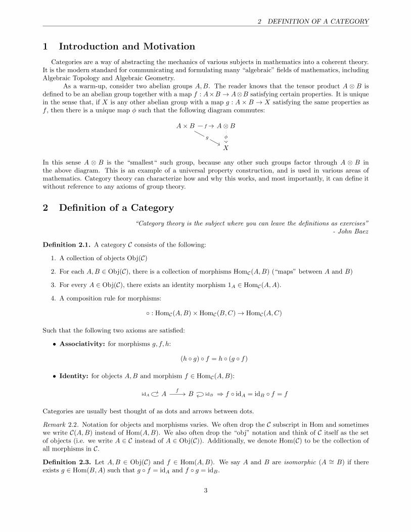
As a warm-up, consider two abelian groups A,B. The reader knows that the tensor product A ⊗ B isdefined to be an abelian group together with a map f : A×B → A⊗B satisfying certain properties. It is uniquein the sense that, if X is any other abelian group with a map g : A× B → X satisfying the same properties asf , then there is a unique map φ such that the following diagram commutes:
A×B A⊗B
X
f
g φ
In this sense A ⊗ B is the “smallest“ such group, because any other such groups factor through A ⊗ B inthe above diagram. This is an example of a universal property construction, and is used in various areas ofmathematics. Category theory can characterize how and why this works, and most importantly, it can define itwithout reference to any axioms of group theory.
2 Definition of a Category
“Category theory is the subject where you can leave the definitions as exercises”- John Baez
Definition 2.1. A category C consists of the following:
1. A collection of objects Obj(C)
2. For each A,B ∈ Obj(C), there is a collection of morphisms HomC(A,B) (“maps” between A and B)
3. For every A ∈ Obj(C), there exists an identity morphism 1A ∈ HomC(A,A).
4. A composition rule for morphisms:
◦ : HomC(A,B)×HomC(B,C)→ HomC(A,C)
Such that the following two axioms are satisfied:
• Associativity: for morphisms g, f, h:
(h ◦ g) ◦ f = h ◦ (g ◦ f)
• Identity: for objects A,B and morphism f ∈ HomC(A,B):
A BidA
fidB ⇒ f ◦ idA = idB ◦ f = f
Categories are usually best thought of as dots and arrows between dots.
Remark 2.2. Notation for objects and morphisms varies. We often drop the C subscript in Hom and sometimeswe write C(A,B) instead of Hom(A,B). We also often drop the “obj” notation and think of C itself as the setof objects (i.e. we write A ∈ C instead of A ∈ Obj(C)). Additionally, we denote Hom(C) to be the collection ofall morphisms in C.
Definition 2.3. Let A,B ∈ Obj(C) and f ∈ Hom(A,B). We say A and B are isomorphic (A ∼= B) if thereexists g ∈ Hom(B,A) such that g ◦ f = idA and f ◦ g = idB .
3
2.1 Examples 3 FUNCTORS
2.1 Examples
Below are some familiar examples of categories.
B Sets (Set), where Obj(Set) are sets and morphisms are functions between sets.
B Groups (Grp), where Obj(Grp) are groups and morphisms are group homomorphisms.
B Modules (Rmod), where Obj(Rmod) are R modules and morphisms are linear homomorphisms
B Topological spaces (Top), where Obj(Top) are topological spaces and morphisms are continuous functions.
B Pointed topological spaes (Top∗), where Obj(Top∗) are spaces with a specified basepoint and morphismsare continuous maps that send basepoints to basepoints.
B The trivial category, 1. This is the category with only one object (often denoted “ · ”) and its identitymorphism.
Definition 2.4. Given a category C, we define the dual (or opposite) category Cop as the category whose objectsare those of C and f ∈ C(A,B) ⇐⇒ f ∈ Cop(B,A). It is the same category but with arrows (morphisms)pointed in the reversed direction.
3 Functors
Definition 3.1. A (covariant) functor F : A → B between categories is a function taking objects in A to objectsin B. Further it maps morphisms to morphisms in the following way:
f ∈ A(A,A′)⇒ F (f) ∈ B(F (A), F (A′))
Further, F must satisfy two conditions:
1. F (g ◦ f) = F (g) ◦ F (f).
2. F (idA) = idF (a).
Remark 3.2. Consider the category of categories (called Cat) : the objects are categories and the morphismsare functors. This allows us to compose functors and declare when two categories are equivalent. Two categoriesare equivalent if they are isomorphic as elements of Cat.
Examples:
• Forgetful functors – functors that “forget” certain information about objects in a category:
a) F : Grp→ Set sending groups to their underlying groups and homomorphisms to maps of sets.
b) F : Ring→ Grp sending rings to their abelian group and homomorphisms to homomorphisms.
• F : AbGrp→ Grp sending groups to themselves, forgetting that they are abelian.
• The fundamental group – This sends a topological space to its fundamental group:
π1 : Top∗ → Grp
• Singular homology – This sends a topological space to its nth singular homology group:
Hn(−) : Top→ AbGrp
Definition 3.3. A contravariant functor is a covariant functor F : Aop → B.
Definition 3.4. A functor F : A → B is faithful if, given A,A′ ∈ Obj(A) then F as a map of A(A′, A) isinjective.
Definition 3.5. A subcategory C of a category A is a category such that:
• Obj(C) ⊂ Obj(A)
• C(C,C ′) ⊂ A(C,C ′)
A subcategory is called full if ∀A,A′ ∈ Obj(A) we have C(A,A′) = A(A,A′).
4
3.1 Natural Transformations 3 FUNCTORS
3.1 Natural Transformations
Consider two functors F,G : A → B. We would like a way to make these compatible:
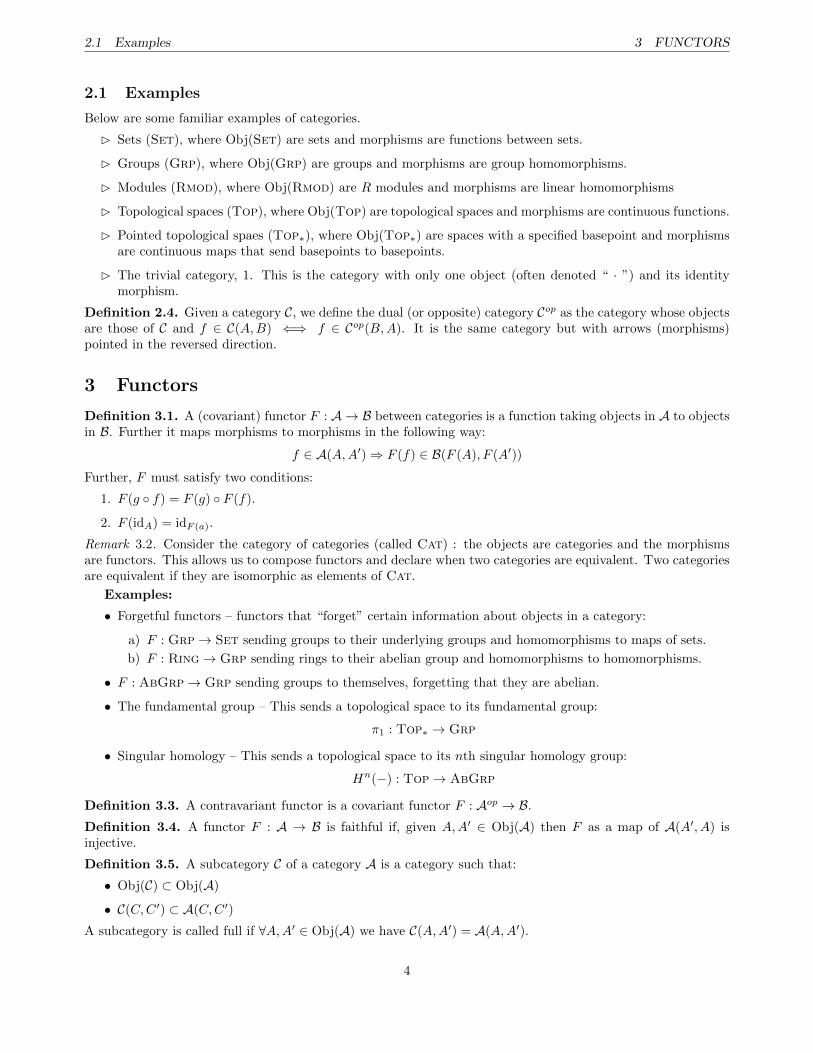
Definition 3.6. A natural transformation N between two functors is a family of morphisms, each of whichassociates an object of A to a morphism N(A) (sometimes denoted NA) of B. Any natural transformation mustmake the following square commute:
F (A) F (A′)
G(A) G(A′)
F (f)
N(A) N(A′)
G(f)
Natural transformations are often denoted as double arrows:
A B
F
G
N
If NA is an isomorphism for each A, then we call N an isomorphism of functors.Examples:
• Let G be a group thought of as a one-object category. A functor F : G → Set gives a group action on aset S. A natural transformation of group actions is a map of sets that respects the group action. Expand
• Let Mn(−) : CRing → Monoid be the functor sending a commutative ring to the monoid of matricesover that ring. Let U : Cring → Monoid be the forgetful functor that forgets ring addition. A naturaltransformation between Mn(−) and U is the determinant. Fix
Remark 3.7. Natural transformations can compose to form another natural transformation. This allows us todefine the functor category:
Definition 3.8. For fixed categories A,B the functor category [A,B] is the category whose objects are functorsA → B and whose morphisms are natural transformations.
Definition 3.9. We say two functors are naturally isomorphic if they are isomorphic as objects in the functorcategory. Equivalently, F,G : A → B are naturally isomorphic if there is a natural transformation α : F → Gsuch that αA : F (A)→ G(A) is an isomorphism for all A ∈ A (such an α is called a natural isomorphism).
3.2 Adjoint Functors
Definition 3.10. Let F : A B : G be functors. We say F is left adjoint to G (and G is right adjoint to F ) iffor every A ∈ A, B ∈ B we have a natural isomorphism:
B(F (A), B) ∼= A(A,G(B))
In other words, this is a natural bijection. For g ∈ B(F (A), B), we denote the corresponding element ofA(A,G(B)) as g.
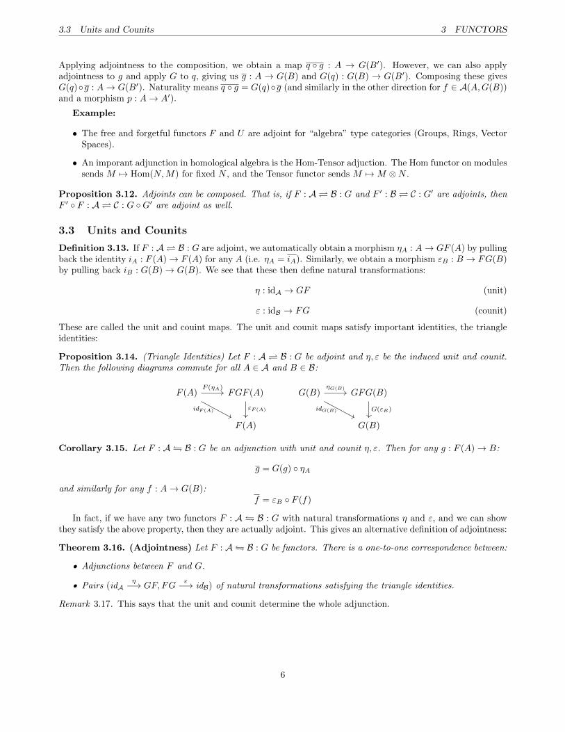
Remark 3.11. The use of “natural” above means something specific: it means the isomorphism is compatiblewith changing A and B. More concretely, if g ∈ B(F (A), B) and we have some morphism q : B → B′, weconsider the composition:
F (A) B B′g
q◦g
q
5
3.3 Units and Counits 3 FUNCTORS
Applying adjointness to the composition, we obtain a map q ◦ g : A → G(B′). However, we can also applyadjointness to g and apply G to q, giving us g : A → G(B) and G(q) : G(B) → G(B′). Composing these givesG(q)◦g : A→ G(B′). Naturality means q ◦ g = G(q)◦g (and similarly in the other direction for f ∈ A(A,G(B))and a morphism p : A→ A′).
Example:
• The free and forgetful functors F and U are adjoint for “algebra” type categories (Groups, Rings, VectorSpaces).
• An imporant adjunction in homological algebra is the Hom-Tensor adjuction. The Hom functor on modulessends M 7→ Hom(N,M) for fixed N , and the Tensor functor sends M 7→M ⊗N .
Proposition 3.12. Adjoints can be composed. That is, if F : A B : G and F ′ : B C : G′ are adjoints, thenF ′ ◦ F : A C : G ◦G′ are adjoint as well.
3.3 Units and Counits
Definition 3.13. If F : A B : G are adjoint, we automatically obtain a morphism ηA : A→ GF (A) by pullingback the identity iA : F (A)→ F (A) for any A (i.e. ηA = iA). Similarly, we obtain a morphism εB : B → FG(B)by pulling back iB : G(B)→ G(B). We see that these then define natural transformations:
η : idA → GF (unit)
ε : idB → FG (counit)
These are called the unit and couint maps. The unit and counit maps satisfy important identities, the triangleidentities:
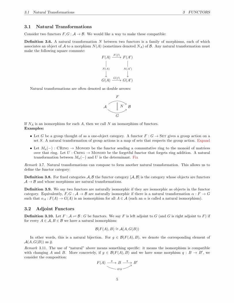
Proposition 3.14. (Triangle Identities) Let F : A B : G be adjoint and η, ε be the induced unit and counit.Then the following diagrams commute for all A ∈ A and B ∈ B:
F (A) FGF (A)
F (A)
F (ηA)
idF (A) εF (A)
G(B) GFG(B)
G(B)
ηG(B)
idG(B) G(εB)
Corollary 3.15. Let F : A� B : G be an adjunction with unit and counit η, ε. Then for any g : F (A)→ B:
g = G(g) ◦ ηA
and similarly for any f : A→ G(B):f = εB ◦ F (f)
In fact, if we have any two functors F : A � B : G with natural transformations η and ε, and we can showthey satisfy the above property, then they are actually adjoint. This gives an alternative definition of adjointness:
Theorem 3.16. (Adjointness) Let F : A� B : G be functors. There is a one-to-one correspondence between:
• Adjunctions between F and G.
• Pairs (idAη−→ GF,FG
ε−→ idB) of natural transformations satisfying the triangle identities.
Remark 3.17. This says that the unit and counit determine the whole adjunction.
6
3.4 Initial and Terminal Objects 3 FUNCTORS
3.4 Initial and Terminal Objects
Definition 3.18. In any category A, there are two special objects:
• An initial object I ∈ A is one so that there exists exactly one morphism I → A for all A ∈ A.
• A terminal object T ∈ A is one so that there exists exactly one morphism A→ T for all A ∈ A.
Examples:
• In Set, the inital object is ∅, and the terminal object is the singleton set {e} for any e.
• In Grp, the initial object is the trivial group {1} and the terminal object is also the trivial group {1}.
• In CRing, the inital object Z and the terminal object is {0}, the zero ring.
Proposition 3.19. Initial and terminal objects are unique up to isomorphism.
We will define adjoint functors using initial and terminal objects. To do this, we must define the commacategory and explain some of its variants.
3.4.1 Comma Categories
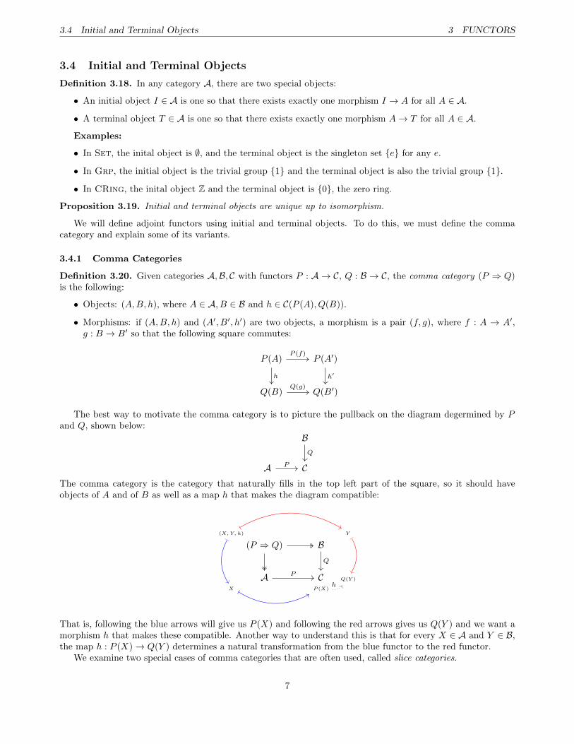
Definition 3.20. Given categories A,B, C with functors P : A → C, Q : B → C, the comma category (P ⇒ Q)is the following:
• Objects: (A,B, h), where A ∈ A, B ∈ B and h ∈ C(P (A), Q(B)).
• Morphisms: if (A,B, h) and (A′, B′, h′) are two objects, a morphism is a pair (f, g), where f : A → A′,g : B → B′ so that the following square commutes:
P (A) P (A′)
Q(B) Q(B′)
P (f)
h h′
Q(g)
The best way to motivate the comma category is to picture the pullback on the diagram degermined by Pand Q, shown below:
B
A C
Q
P
The comma category is the category that naturally fills in the top left part of the square, so it should haveobjects of A and of B as well as a map h that makes the diagram compatible:
(X, Y, h) Y
(P ⇒ Q) B
A C Q(Y )
X P (X)
Q
P
h
That is, following the blue arrows will give us P (X) and following the red arrows gives us Q(Y ) and we want amorphism h that makes these compatible. Another way to understand this is that for every X ∈ A and Y ∈ B,the map h : P (X)→ Q(Y ) determines a natural transformation from the blue functor to the red functor.
We examine two special cases of comma categories that are often used, called slice categories.
7
4 REPRESENTABILITY AND YONEDA’S LEMMA
Definition 3.21. Given a category A and an object A ∈ A, the slice category, denote A/A, is the commacategory on the functors idA : A → A and (·) : 1 → A, the first of which is the identity, and the second sendsthe singleton object · identically to A. Explicitly, the slice category is:
• Objects: (X,h) for X ∈ A and h : X → A.
• Morphisms: f : X → X ′ so that the diagram commutes:
X X ′
A
f
h h′
The second is a more general version of the slice category, where instead of the identity idA : A → A, wehave an arbitrary functor G : B → A. This is also sometimes known as the slice category and has an equivalentformulation as above. This slice category is denoted (A⇒ G).
———————
Now we return to initial and terminal objects and their relationship to adjoint functors.
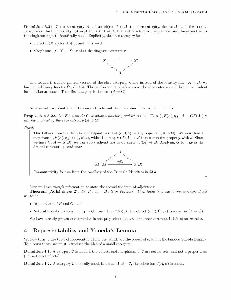
Proposition 3.22. Let F : A � B : G be adjoint functors, and let A ∈ A. Then (·, F (A), ηA : A→ GF (A)) isan initial object of the slice category (A⇒ G).
Proof:
This follows from the definition of adjointness. Let (·, B, h) be any object of (A⇒ G). We must find amap from (·, F (A), ηA) to (·, B, h), which is a map h : F (A)→ B that commutes properly with h. Sincewe have h : A → G(B), we can apply adjointness to obtain h : F (A) → B. Applying G to h gives thedesired commuting condition:
A
GF (A) G(B)
ηA h
G(h)
Commutativity follows from the corollary of the Triangle Identities in §3.3.
�
Now we have enough information to state the second theorem of adjointness:Theorem (Adjointness 2). Let F : A � B : G be functors. Then there is a one-to-one correspondnece
bewteen:
• Adjunctions of F and G, and
• Natural transformations η : idA → GF such that ∀A ∈ A, the object (·, F (A), ηA) is initial in (A⇒ G).
We have already proven one direction in the proposition above. The other direction is left as an exercise.
4 Representability and Yoneda’s Lemma
We now turn to the topic of representable functors, which are the object of study in the famous Yoneda Lemma.To discuss these, we must introduce the idea of a small category.
Definition 4.1. A category C is small if the objects and morphisms of C are actual sets, and not a proper class(i.e. not a set of sets).
Definition 4.2. A category C is locally small if, for all A,B ∈ C, the collection C(A,B) is small.
8
4.1 Representables 4 REPRESENTABILITY AND YONEDA’S LEMMA
Examples:
• The trivial category 1 is small.
• Set is not small, but it is locally small.
Since most of the categories we work with are built from sets (groups, rings, modules, etc.), most of our commmonexamples are not small, but are locally small.
4.1 Representables
Let C be a locally small category, and let A ∈ C. Then we define the functor HA : C → Set given by B 7→ C(A,B).This acts on morphisms via precomposition, i.e. HA(g : B → B′) = g ◦ (·).
Definition 4.3. Let X : A → Set be a covariant a functor. It is called representable if X ∼= HA naturally forsome A ∈ A1. If α : HA → X is an isomorphism, we sometimes call (A,α) a representation of X.
Examples:
• (Diagonal) Consider the functor ∆ : Set → Set given by S 7→ S × S, and f 7→ (f, f). This can berepresented by the set {0, 1} = 2. To see this, note that an element of Hom({0, 1}, S) is determined exactlyby choosing where to send 0 and 1, so it is indeed isomorphic to S × S = ∆S.
• (Powersets) The powerset functor P : Setop → Set sends a set to its powerset, and sends maps f :S → T to the map sending X ⊂ T to f−1(X). It turns out that P can also be represented using theobject {0, 1}. First we note that HomSetop({0, 1}, S) = HomSet(S, {0, 1}), so we must demonstrate anisomorphism P(S) ∼= HomSet(S, {0, 1}). This is given by sending a subset X ⊂ S to its indicator functionχS : S → {0, 1}.
• (Tensor products) Let M and N be R−modules. Then the bilinear functor Bilin(M,N ;−) : Rmod→ Setsends a module P to the set of bilinear maps g : M×N → P and sends a module map f to post-compositionwith f . Then, by the universal property of the tensor product, we have Bilin(M,N ;P ) ∼= Hom(M⊗RN,P )and so this functor can be represented using the tensor product M⊗RN .
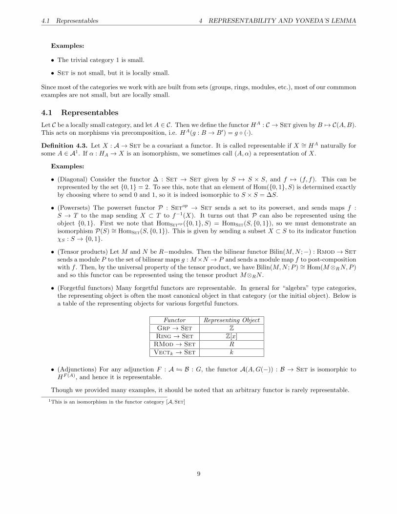
• (Forgetful functors) Many forgetful functors are representable. In general for “algebra” type categories,the representing object is often the most canonical object in that category (or the initial object). Below isa table of the representing objects for various forgetful functors.
Functor Representing ObjectGrp → Set ZRing → Set Z[x]RMod → Set RVectk → Set k
• (Adjunctions) For any adjunction F : A � B : G, the functor A(A,G(−)) : B → Set is isomorphic toHF (A), and hence it is representable.
Though we provided many examples, it should be noted that an arbitrary functor is rarely representable.
1This is an isomorphism in the functor category [A,Set]
9
4.2 The Yoneda Embedding 4 REPRESENTABILITY AND YONEDA’S LEMMA
4.2 The Yoneda Embedding
Suppose we have a morphism f : A → A′; then we obtain a natural transformation ηf : HA′ → HA given byprecomposing with f . This allows us to define a new functor:
H• : Cop → [C,Set]
A 7→ HA
f 7→ ηf
This is an “embedding” of Cop as a collection of functors from C to Set (also called copresheaves).We can dualize this whole discussion and define the functor HA : Cop → Set for A ∈ C. This is given by
B 7→ C(B,A) and postcomposition on morphisms. We say that a functor X : Cop → Set (also called a presheaf)is corepresentable if X ∼= HA for some A. Similarly to before, we have a functor:
H• : C → [Cop,Set]
A 7→ HA
f 7→ εf
Where ε is the equivalent natural transformation to η above. This is an embedding of C as a collection ofpresheaves, also called the Yoneda embedding.
4.3 The Yoneda Lemma
Let C be locally small and let X : Cop → Set be a presheaf. We can ask how X is related to a representingfunctor HA for any A ∈ C. More specifically, we can ask how is X “seen” by HA. In other words, what doesthe set of natural transformations HA ⇒ X look like? In the language of the functor category [Cop,Set], thismeans we want to understand [Cop,Set](HA, X) as a set.
Exercise: Convince yourself that in the case of a representable presheafX ∼= HB , we have [Cop,Set](HA, X) ∼=C(A,B).
We note that, in the special case above of X ∼= HB , it happens that [Cop,Set](HA, X) = X(A). This turnsout to be true even if X is not representable. This is the Yoneda Lemma:
Lemma 4.4. (Yoneda) If X : Cop → Set is a presheaf on a locally small category, then for any A ∈ C:
[Cop,Set](HA, X) ∼= X(A) (Naturally in X and A)
In other words, the set of natural transformations HA ⇒ X is in one-to-one correspondence with elements ofX(A).
Proof:
This will proceed by explicitly constructing maps in both directions that compose to the identity. Inone direction, we wish to associate to a natural transformation α : HA ⇒ X an element of X(A). The“only” choice we have is to use the data that the natural transformation provides, namely a morphismαA : HA(A) → X(A). Since HA(A) = C(A,A), we can pick 1A ∈ C(A,A) and look at is image underαA. Thus, we have a map:
( ) : [Cop,Set](HA, X)→ X(A)
α 7→ αA(1A) := α
In the other direction, we wish to associate to any element x ∈ X(A) a natural transformation x. Forany B ∈ C, we must define a morphism xB : HA(B)→ X(B). The natural way to define this morphismis f 7→ X(f)(x). Thus we have another map:
( ˜ ) : X(A)→ [Cop,Set](HA, X)
x 7→ (f 7→ X(f)(x)) := x
10
4.4 Consequences of Yoneda 4 REPRESENTABILITY AND YONEDA’S LEMMA
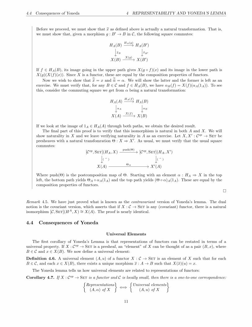
Before we proceed, we must show that x as defined above is actually a natural transformation. That is,we must show that, given a morphism g : B′ → B in C, the following square commutes:
HA(B) HA(B′)
X(B) X(B′)
HA(g)
xB xB′
X(g)
If f ∈ HA(B), its image going in the upper path gives X(g ◦ f)(x) and its image in the lower path isX(g)(X(f)(x)). Since X is a functor, these are equal by the composition properties of functors.
Now we wish to show that x = x and ˜α = α. We will show the latter and the former is left as anexercise. We must verify that, for any B ∈ C and f ∈ HA(B), we have αB(f) = X(f)(αA(1A)). To seethis, consider the commuting square we get from α being a natural transformation:
HA(A) HA(B)
X(A) X(B)
HA(f)
αA αB
X(f)
If we look at the image of 1A ∈ HA(A) through both paths, we obtain the desired result.The final part of this proof is to verify that this isomorphism is natural in both A and X. We will
show naturality in X and we leave verifying naturality in A as an exercise. Let X,X ′ : Cop → Set bepresheaves with a natural transfomration Θ : X ⇒ X ′. As usual, we must verify that the usual squarecommutes:
[Cop,Set](HA, X) [Cop,Set](HA, X′)
X(A) X ′(A)
push(Θ)
( ) ( )
ΘA
Where push(Θ) is the postcomposition map of Θ. Starting with an element α : HA ⇒ X in the topleft, the bottom path yields ΘA ◦ αA(1A) and the top path yields (Θ ◦ α)A(1A). These are equal by thecomposition properties of functors.
�
Remark 4.5. We have just proved what is known as the contravariant version of Yoneda’s lemma. The dualnotion is the covariant version, which asserts that if X : C → Set is any (covariant) functor, there is a naturalisomorphism [C,Set](HA, X) ∼= X(A). The proof is nearly identical.
4.4 Consequences of Yoneda
Universal Elements
The first corollary of Yoneda’s Lemma is that representations of functors can be restated in terms of auniversal property. If X : Cop → Set is a presheaf, an “element” of X can be thought of as a pair (B, x), whereB ∈ C and x ∈ X(B). We now define a universal element:
Definition 4.6. A universal element (A, u) of a functor X : C → Set is an element of X such that for eachB ∈ C, and each x ∈ X(B), there exists a unique morphism x : A→ B such that X(x)(u) = x.
The Yoneda lemma tells us how universal elements are related to representations of functors:
Corollary 4.7. If X : Cop → Set is a functor and C is locally small, then there is a one-to-one correspondence:{Representations
(A,α) of X
}⇐⇒
{Universal elements
(A, u) of X
}
11
5 LIMITS AND COLIMITS
Proof:
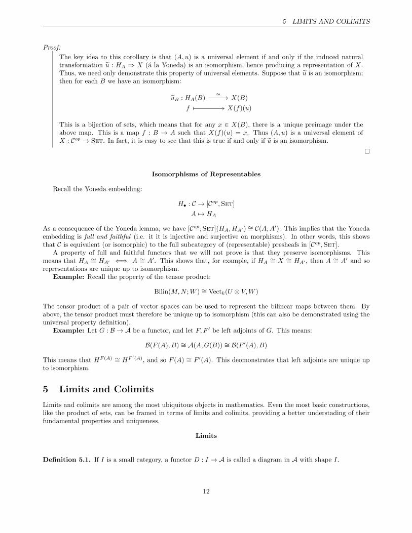
The key idea to this corollary is that (A, u) is a universal element if and only if the induced naturaltransformation u : HA ⇒ X (a la Yoneda) is an isomorphism, hence producing a representation of X.Thus, we need only demonstrate this property of universal elements. Suppose that u is an isomorphism;then for each B we have an isomorphism:
uB : HA(B) X(B)
f X(f)(u)
∼=
This is a bijection of sets, which means that for any x ∈ X(B), there is a unique preimage under theabove map. This is a map f : B → A such that X(f)(u) = x. Thus (A, u) is a universal element ofX : Cop → Set. In fact, it is easy to see that this is true if and only if u is an isomorphism.
�
Isomorphisms of Representables
Recall the Yoneda embedding:
H• : C → [Cop,Set]
A 7→ HA
As a consequence of the Yoneda lemma, we have [Cop,Set](HA, HA′) ∼= C(A,A′). This implies that the Yonedaembedding is full and faithful (i.e. it it is injective and surjective on morphisms). In other words, this showsthat C is equivalent (or isomorphic) to the full subcategory of (representable) presheafs in [Cop,Set].
A property of full and faithful functors that we will not prove is that they preserve isomorphisms. Thismeans that HA
∼= HA′ ⇐⇒ A ∼= A′. This shows that, for example, if HA∼= X ∼= HA′ , then A ∼= A′ and so
representations are unique up to isomorphism.Example: Recall the property of the tensor product:
Bilin(M,N ;W ) ∼= Vectk(U ⊗ V,W )
The tensor product of a pair of vector spaces can be used to represent the bilinear maps between them. Byabove, the tensor product must therefore be unique up to isomorphism (this can also be demonstrated using theuniversal property definition).
Example: Let G : B → A be a functor, and let F, F ′ be left adjoints of G. This means:
B(F (A), B) ∼= A(A,G(B)) ∼= B(F ′(A), B)
This means that HF (A) ∼= HF ′(A), and so F (A) ∼= F ′(A). This deomonstrates that left adjoints are unique upto isomorphism.
5 Limits and Colimits
Limits and colimits are among the most ubiquitous objects in mathematics. Even the most basic constructions,like the product of sets, can be framed in terms of limits and colimits, providing a better understading of theirfundamental properties and uniqueness.
Limits
Definition 5.1. If I is a small category, a functor D : I → A is called a diagram in A with shape I.
12
5.1 (Co)Products, (Co)Equalizers, Pullbacks and Pushouts 5 LIMITS AND COLIMITS
Definition 5.2. Given a category A and a diagram D : I → A, a cone with vertex A ∈ A of shape I is afamily of morphisms ψX : A→ D(X) for each X such that for any morphism f : X → Y , the following diagramcommutes:
D(Y )
A
D(X)
ψY
ψX
D(f)
Remark 5.3. Sometimes we are abusive and we refer to the whole cone by its tip, but implicilty we refer to boththe tip and the morphisms from the tip.
We now define the category of cones with shape D : I → A (or just shape I if we’re lazy) to be the categorywhose objects are cones of shape D : I → A and whose morphisms are morphisms between the vertices of thecones. Maps between tips must commute.
Definition 5.4. The limit of a diagram D : I → A is the terminal object in the category of cones over D. It isusually denoted limI(D).
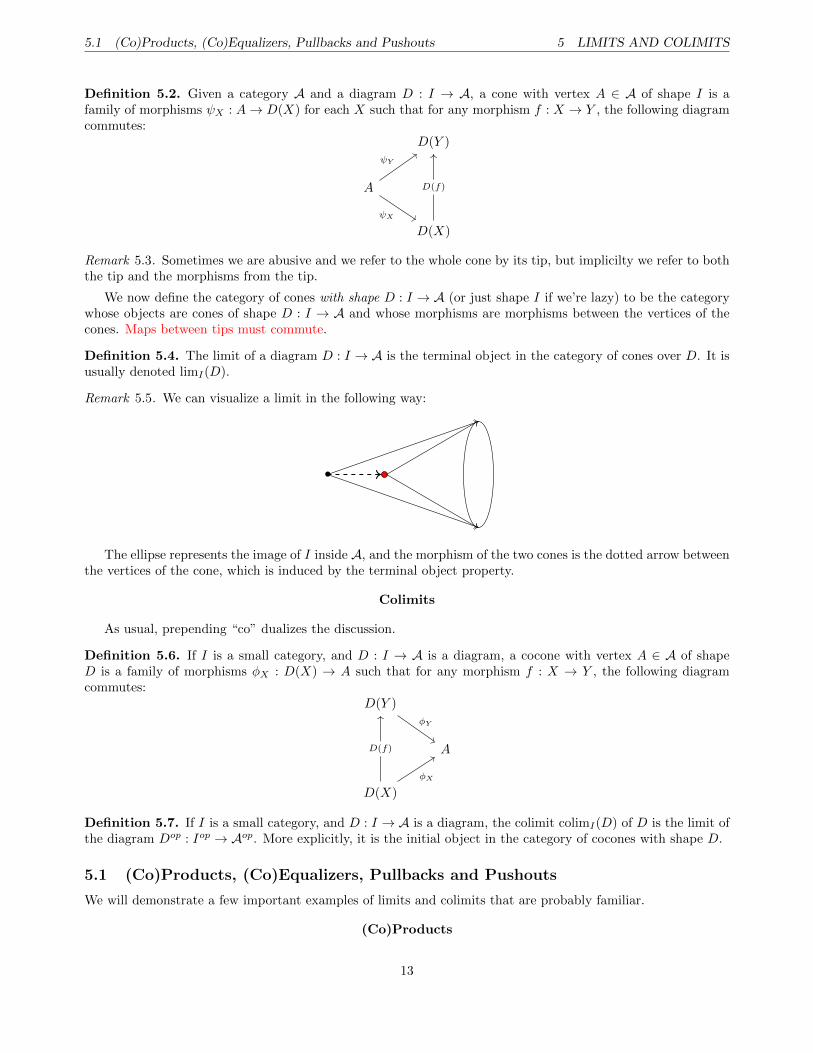
Remark 5.5. We can visualize a limit in the following way:
•
The ellipse represents the image of I inside A, and the morphism of the two cones is the dotted arrow betweenthe vertices of the cone, which is induced by the terminal object property.
Colimits
As usual, prepending “co” dualizes the discussion.
Definition 5.6. If I is a small category, and D : I → A is a diagram, a cocone with vertex A ∈ A of shapeD is a family of morphisms φX : D(X) → A such that for any morphism f : X → Y , the following diagramcommutes:
D(Y )
A
D(X)
φY
D(f)
φX
Definition 5.7. If I is a small category, and D : I → A is a diagram, the colimit colimI(D) of D is the limit ofthe diagram Dop : Iop → Aop. More explicitly, it is the initial object in the category of cocones with shape D.
5.1 (Co)Products, (Co)Equalizers, Pullbacks and Pushouts
We will demonstrate a few important examples of limits and colimits that are probably familiar.
(Co)Products
13
5.1 (Co)Products, (Co)Equalizers, Pullbacks and Pushouts 5 LIMITS AND COLIMITS
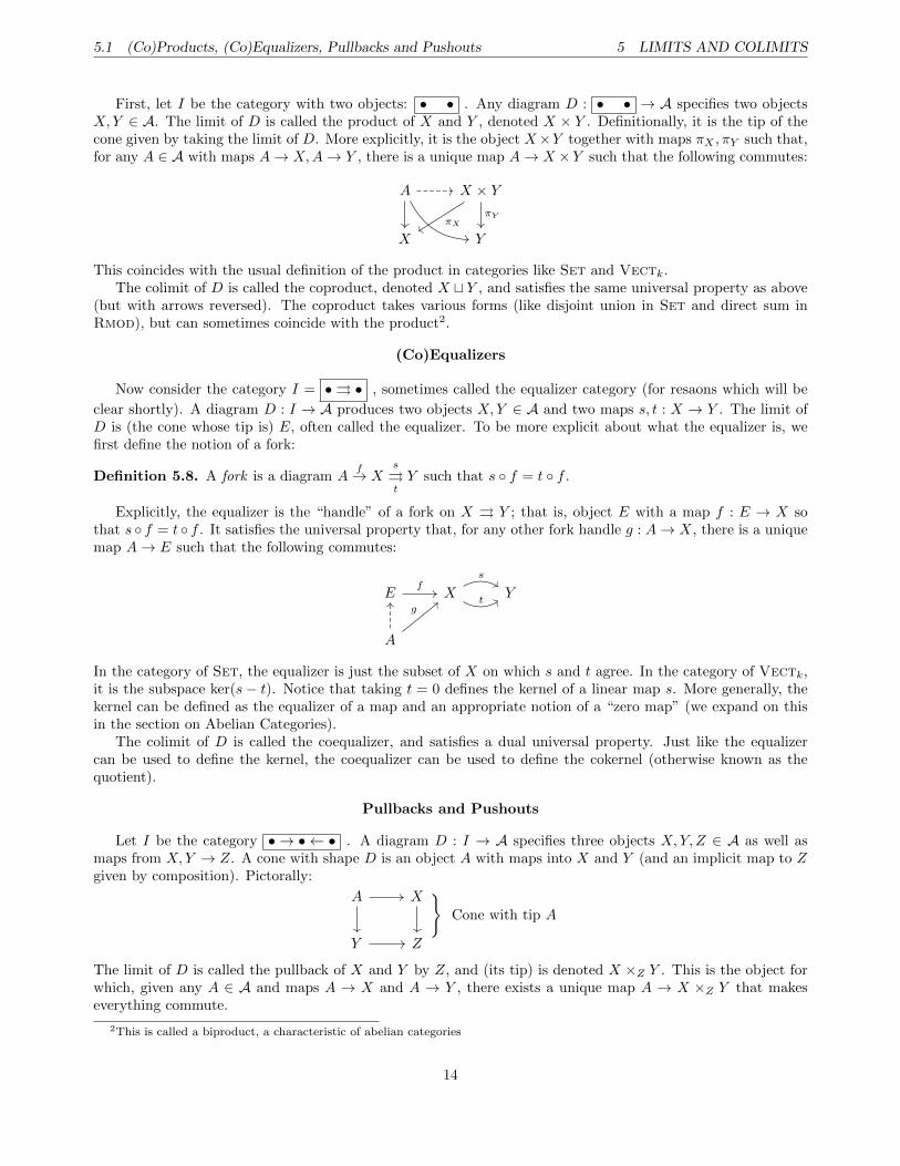
First, let I be the category with two objects: • • . Any diagram D : • • → A specifies two objectsX,Y ∈ A. The limit of D is called the product of X and Y , denoted X × Y . Definitionally, it is the tip of thecone given by taking the limit of D. More explicitly, it is the object X×Y together with maps πX , πY such that,for any A ∈ A with maps A→ X,A→ Y , there is a unique map A→ X ×Y such that the following commutes:
A X × Y
X Y
πX
πY
This coincides with the usual definition of the product in categories like Set and Vectk.The colimit of D is called the coproduct, denoted X t Y , and satisfies the same universal property as above
(but with arrows reversed). The coproduct takes various forms (like disjoint union in Set and direct sum inRmod), but can sometimes coincide with the product2.
(Co)Equalizers
Now consider the category I = •⇒ • , sometimes called the equalizer category (for resaons which will be
clear shortly). A diagram D : I → A produces two objects X,Y ∈ A and two maps s, t : X → Y . The limit ofD is (the cone whose tip is) E, often called the equalizer. To be more explicit about what the equalizer is, wefirst define the notion of a fork:
Definition 5.8. A fork is a diagram Af→ X
s
⇒tY such that s ◦ f = t ◦ f .
Explicitly, the equalizer is the “handle” of a fork on X ⇒ Y ; that is, object E with a map f : E → X sothat s ◦ f = t ◦ f . It satisfies the universal property that, for any other fork handle g : A→ X, there is a uniquemap A→ E such that the following commutes:
E X Y
A
fs
tg
In the category of Set, the equalizer is just the subset of X on which s and t agree. In the category of Vectk,it is the subspace ker(s− t). Notice that taking t = 0 defines the kernel of a linear map s. More generally, thekernel can be defined as the equalizer of a map and an appropriate notion of a “zero map” (we expand on thisin the section on Abelian Categories).
The colimit of D is called the coequalizer, and satisfies a dual universal property. Just like the equalizercan be used to define the kernel, the coequalizer can be used to define the cokernel (otherwise known as thequotient).
Pullbacks and Pushouts
Let I be the category • → • ← • . A diagram D : I → A specifies three objects X,Y, Z ∈ A as well asmaps from X,Y → Z. A cone with shape D is an object A with maps into X and Y (and an implicit map to Zgiven by composition). Pictorally:
A X
Y Z
}Cone with tip A
The limit of D is called the pullback of X and Y by Z, and (its tip) is denoted X ×Z Y . This is the object forwhich, given any A ∈ A and maps A → X and A → Y , there exists a unique map A → X ×Z Y that makeseverything commute.
2This is called a biproduct, a characteristic of abelian categories
14
5.2 Topological limits 5 LIMITS AND COLIMITS
In the category of Set, the pullback has an easy interpretation. If we have set-maps f : X → Z andg : Y → Z, the pullback is:
X ×Z Y = {(x, y) ∈ X × Y | f(x) = g(y)}
In the case where both X and Y are inside Z (and f and g are given by inclusion), then the pullback is(isomorphic to) the intersection of the sets, X ∩ Y .
The colimit of D is called the pushout, denoted X tZ Y , and satisfies a universal property dual to the oneabove. In the category of sets, this can be explicitly written as:
X tZ Y = X t Y/ ∼
Where X tY is the disjoint union, and a ∼ b if they share a preimage inside Z under f : Z → X and g : Z → Y .In the case where Z = X ∩ Y and f and g are inclusion, the pushout is the union X ∪ Y .
Example: The 2-sphere S2 can be constructed using an equalizer. Let A be the category of topological
spaces, and consider the equalizer of R31⇒t
R, where t(x, y, z) = x2 + y2 + z2 and 1(x, y, z) = 1. Then the
equalizer of this diagram is the unit sphere defined implicitly via coordinates:
{(x, y, z) | x2 + y2 + z2 = 1}
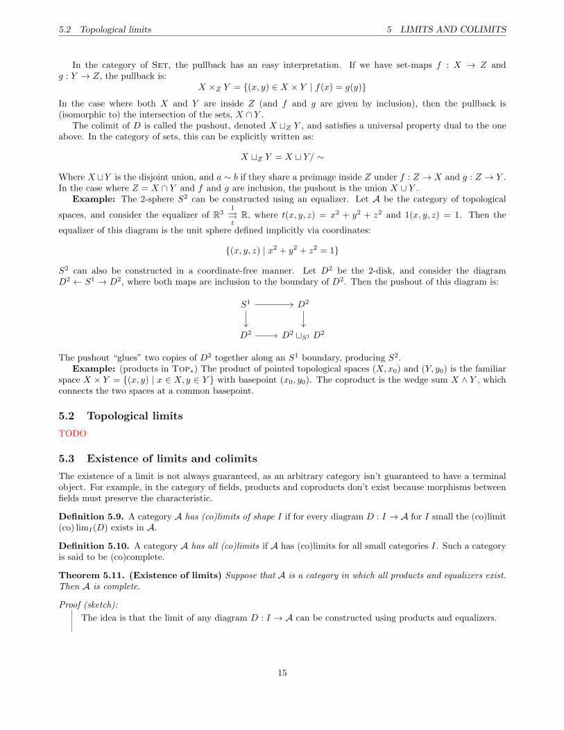
S2 can also be constructed in a coordinate-free manner. Let D2 be the 2-disk, and consider the diagramD2 ← S1 → D2, where both maps are inclusion to the boundary of D2. Then the pushout of this diagram is:
S1 D2
D2 D2 tS1 D2
The pushout “glues” two copies of D2 together along an S1 boundary, producing S2.Example: (products in Top∗) The product of pointed topological spaces (X,x0) and (Y, y0) is the familiar
space X × Y = {(x, y) | x ∈ X, y ∈ Y } with basepoint (x0, y0). The coproduct is the wedge sum X ∧ Y , whichconnects the two spaces at a common basepoint.
5.2 Topological limits
TODO
5.3 Existence of limits and colimits
The existence of a limit is not always guaranteed, as an arbitrary category isn’t guaranteed to have a terminalobject. For example, in the category of fields, products and coproducts don’t exist because morphisms betweenfields must preserve the characteristic.
Definition 5.9. A category A has (co)limits of shape I if for every diagram D : I → A for I small the (co)limit(co) limI(D) exists in A.
Definition 5.10. A category A has all (co)limits if A has (co)limits for all small categories I. Such a categoryis said to be (co)complete.
Theorem 5.11. (Existence of limits) Suppose that A is a category in which all products and equalizers exist.Then A is complete.
Proof (sketch):
The idea is that the limit of any diagram D : I → A can be constructed using products and equalizers.
15
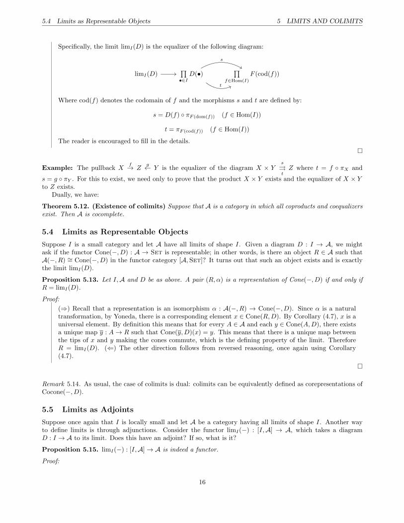
5.4 Limits as Representable Objects 5 LIMITS AND COLIMITS
Specifically, the limit limI(D) is the equalizer of the following diagram:
limI(D)∏•∈I
D(•)∏
f∈Hom(I)
F (cod(f))
s
t
Where cod(f) denotes the codomain of f and the morphisms s and t are defined by:
s = D(f) ◦ πF (dom(f)) (f ∈ Hom(I))
t = πF (cod(f)) (f ∈ Hom(I))
The reader is encouraged to fill in the details.
�
Example: The pullback Xf→ Z
g← Y is the equalizer of the diagram X × Ys⇒tZ where t = f ◦ πX and
s = g ◦ πY . For this to exist, we need only to prove that the product X × Y exists and the equalizer of X × Yto Z exists.
Dually, we have:
Theorem 5.12. (Existence of colimits) Suppose that A is a category in which all coproducts and coequalizersexist. Then A is cocomplete.
5.4 Limits as Representable Objects
Suppose I is a small category and let A have all limits of shape I. Given a diagram D : I → A, we mightask if the functor Cone(−, D) : A → Set is representable; in other words, is there an object R ∈ A such thatA(−, R) ∼= Cone(−, D) in the functor category [A,Set]? It turns out that such an object exists and is exactlythe limit limI(D).
Proposition 5.13. Let I,A and D be as above. A pair (R,α) is a representation of Cone(−, D) if and only ifR = limI(D).
Proof:
(⇒) Recall that a representation is an isomorphism α : A(−, R) → Cone(−, D). Since α is a naturaltransformation, by Yoneda, there is a corresponding element x ∈ Cone(R,D). By Corollary (4.7), x is auniversal element. By definition this means that for every A ∈ A and each y ∈ Cone(A,D), there existsa unique map y : A→ R such that Cone(y,D)(x) = y. This means that there is a unique map betweenthe tips of x and y making the cones commute, which is the defining property of the limit. ThereforeR = limI(D). (⇐) The other direction follows from reversed reasoning, once again using Corollary(4.7).
�
Remark 5.14. As usual, the case of colimits is dual: colimits can be equivalently defined as corepresentations ofCocone(−, D).
5.5 Limits as Adjoints
Suppose once again that I is locally small and let A be a category having all limits of shape I. Another wayto define limits is through adjunctions. Consider the functor limI(−) : [I,A] → A, which takes a diagramD : I → A to its limit. Does this have an adjoint? If so, what is it?
Proposition 5.15. limI(−) : [I,A]→ A is indeed a functor.
Proof:
16
5.5 Limits as Adjoints 5 LIMITS AND COLIMITS
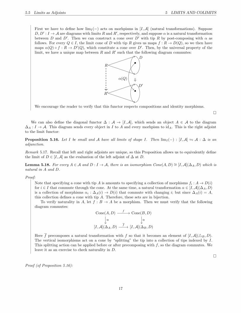
First we have to define how limI(−) acts on morhpisms in [I,A] (natural transformations). SupposeD,D′ : I → A are diagrams with limits R and R′, respectively, and suppose α is a natural transformationbetween D and D′. Then we can construct a cone over D′ with tip R by post-composing with α asfollows. For every Q ∈ I, the limit cone of D with tip R gives us maps f : R→ D(Q), so we then havemaps α(Q) ◦ f : R → D′(Q), which constitute a cone over D′. Then, by the universal property of thelimit, we have a unique map between R and R′ such that the following diagram commutes:
R
D
R′
D′⇓
•
•
α(Q)
We encourage the reader to verify that this functor respects compositions and identity morphisms.
�
We can also define the diagonal functor ∆ : A → [I,A], which sends an object A ∈ A to the diagram∆A : I → A. This diagram sends every object in I to A and every morhpism to idA. This is the right adjointto the limit functor:
Proposition 5.16. Let I be small and A have all limits of shape I. Then limI(−) : [I,A] � A : ∆ is anadjunction.
Remark 5.17. Recall that left and right adjoints are unique, so this Proposition allows us to equivalently definethe limit of D ∈ [I,A] as the evaluation of the left adjoint of ∆ at D.
Lemma 5.18. For every A ∈ A and D : I → A, there is an isomorphism Cone(A,D) ∼= [I,A](∆A, D) which isnatural in A and D.
Proof:
Note that specifying a cone with tip A is amounts to specifying a collection of morphisms fi : A→ D(i)for i ∈ I that commute through the cone. At the same time, a natural transformation α ∈ [I,A](∆A, D)is a collection of morphisms αi : ∆A(i) → D(i) that commute with changing i; but since ∆A(i) = A,this collection defines a cone with tip A. Therefore, these sets are in bijection.
To verify naturality in A, let f : B → A be a morphism. Then we must verify that the followingdiagram commutes:
Cone(A,D) Cone(B,D)
[I,A](∆A, D) [I,A](∆B , D)
∼=
f
∼=f
Here f precomposes a natural transformation with f so that it becomes an element of [I,A](4B , D).The vertical isomorphisms act on a cone by “splitting” the tip into a collection of tips indexed by I.This splitting action can be applied before or after precomposing with f , so the diagram commutes. Weleave it as an exercise to check naturality in D.
�
Proof (of Proposition 5.16):
17
5.6 Preserving Limits and GAFT 5 LIMITS AND COLIMITS
Let A ∈ A and D : I → A be a diagram. Recall from Proposition 5.13 that A(−, limI(D)) ∼= Cone(−, D),which means there is a natural transformation α that is an isomorphism when restricted to every objectin in A. Therefore α(A) : A(A, limI(D)) → Cone(A,D) is a natural isomorphism. By the previousLemma, we then have:
[I,A](∆A, D) ∼= Cone(A,D) ∼= A(A, limI
(D))
Further, these are natural isomorphisms. Therefore limI(−) and ∆ are adjoints.
�
5.6 Preserving Limits and GAFT
Much like with classical limits in calculus and analysis, a central question about categorical limits is if theycommute with various operations. For example, for what types of functors F does F (limI(D)) equal limI(F ◦D)?In this section we’ll address prove two classes of functors for which this is true, as well as describe a partialconverse to one of these. TODO.
18
6 ABELIAN CATEGORIES
6 Abelian Categories
Loosely speaking, an abelian cagetory is a type of category that behaves like modules (R-mod) or abelian groups(Ab). We must first define a few types of morphisms that such a category must have.
Definition 6.1. A morphism f : X → Y in a category C is a zero morphism if:
• for any A ∈ C and any g, h : A→ X, fg = fh
• for any B ∈ C and any g, h : Y → B, gf = hf
We denote a zero morphism as 0XY (or sometimes just 0 if the context is sufficient).
Definition 6.2. A morphism f : X → Y is a monomorphism if it is left cancellative. That is, for all g, h : Z → X,we have fg = fh⇒ g = h. A morphism is an epimorphism if it is right cancellative.
The zero morphism is a generalization of the zero map on rings, or the identity homomorphism on groups.Monomorphisms and epimorphisms are generalizations of injective and surjective homomorphisms (though thesedefinitions don’t always coincide). It can be shown that a morphism is an isomorphism iff it is epic and monic.
Definition 6.3. The kernel of a morphism f ∈ C(A,B) is the equalizer of f with 0AB . The cokernel of f is thecoequalizer of f with 0AB .
Definition 6.4. The image of a morphism is the kernel of its cokernel, and the coimage is the cokernel of itskernel.
As the names suggest, the kernel and cokernel are meant to generalize the concepts well-known in groups. Itis easy to show that the kernel of a monomorphism is 0AB and the cokernel of an epimorphism is 0AB ; likewisekernels are monic and cokernels are epic.
Definition 6.5. A category C is called abelian if it satisfies the following properties:
1. It has an object that is both initial and terminal (also called the zero object, denoted 0).
2. It has all pairwise products and coproducts.
3. It has all kernels and cokernels.
4. All monomorphisms (resp. epimorphisms) can be written as the kernel (resp. cokernel) of a morphism.
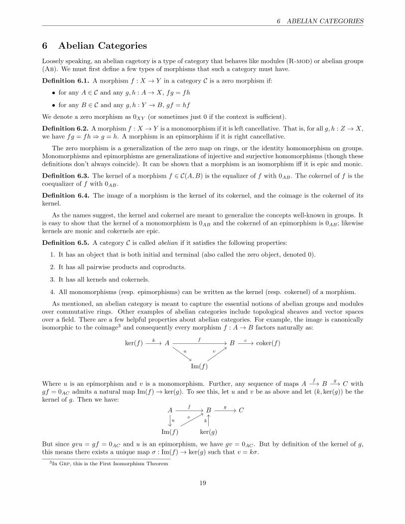
As mentioned, an abelian category is meant to capture the essential notions of abelian groups and modulesover commutative rings. Other examples of abelian categories include topological sheaves and vector spacesover a field. There are a few helpful properties about abelian categories. For example, the image is canonicallyisomorphic to the coimage3 and consequently every morphism f : A→ B factors naturally as:
ker(f) A B coker(f)
Im(f)
k
u
f c
v
Where u is an epimorphism and v is a monomorphism. Further, any sequence of maps Af−→ B
g−→ C withgf = 0AC admits a natural map Im(f)→ ker(g). To see this, let u and v be as above and let (k, ker(g)) be thekernel of g. Then we have:
A B C
Im(f) ker(g)
f
u
g
vk
But since gvu = gf = 0AC and u is an epimorphism, we have gv = 0AC . But by definition of the kernel of g,this means there exists a unique map σ : Im(f)→ ker(g) such that v = kσ.
3In Grp, this is the First Isomorphism Theorem
19
6.1 Homology 6 ABELIAN CATEGORIES
6.1 Homology
Definition 6.6. A sequence Af−→ B
g−→ C with gf = 0AC is called exact if the map σ above is an isomorphism.
The dual definition of exactness can be phrased in terms of the image of g and the cokernel of f :
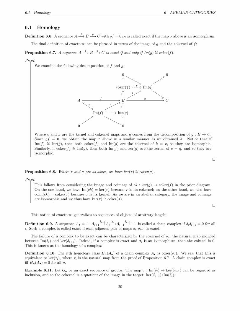
Proposition 6.7. A sequence Af−→ B
g−→ C is exact if and only if Im(g) ∼= coker(f).
Proof:
We examine the following decomposition of f and g:
0 0
coker(f) Im(g)
A B C
Im(f) ker(g)
0 0
τ
f
u
c q
g
v
σ
k
Where c and k are the kernel and cokernel maps and q comes from the decomposition of g : B → C.Since gf = 0, we obtain the map τ above in a similar manner as we obtained σ. Notice that ifIm(f) ∼= ker(g), then both coker(f) and Im(g) are the cokernel of k = v, so they are isomorphic.Similarly, if coker(f) ∼= Im(g), then both Im(f) and ker(g) are the kernel of c = q, and so they areisomorphic.
�
Proposition 6.8. Where τ and σ are as above, we have ker(τ) ∼= coker(σ).
Proof:
This follows from considering the image and coimage of ck : ker(g) → coker(f) in the prior diagram.On the one hand, we have Im(ck) = ker(τ) because τ is its cokernel; on the other hand, we also havecoim(ck) = coker(σ) because σ is its kernel. As we are in an abelian category, the image and coimageare isomorphic and we thus have ker(τ) ∼= coker(σ).
�
This notion of exactness generalizes to sequences of objects of arbitrary length:
Definition 6.9. A sequence A• = · · ·Ai+1δi+1−→Ai
δi−→Ai−1δi−1−→· · · is called a chain complex if δiδi+1 = 0 for all
i. Such a complex is called exact if each adjacent pair of maps δi, δi+1 is exact.
The failure of a complex to be exact can be characterized by the cokernel of σi, the natural map inducedbetween Im(δi) and ker(δi+1). Indeed, if a complex is exact and σi is an isomorphism, then the cokenel is 0.This is known as the homology of a complex:
Definition 6.10. The nth homology class Hn(A•) of a chain complex A• is coker(σi). We saw that this isequivalent to ker(τi), where τi is the natural map from the proof of Proposition 6.7. A chain complex is exactiff Hn(A•) = 0 for all n.
Example 6.11. Let G• be an exact sequence of groups. The map σ : Im(δi) → ker(δi−1) can be regarded asinclusion, and so the cokernel is a quotient of the image in the target: ker(δi−1)/Im(δi).
20
6.1 Homology 6 ABELIAN CATEGORIES
A particular type of exact sequence that we will consider is a short exact sequence 0→ Af−→ B
g−→ C → 0.Here, exactness implies that f is a monomorphism and g is an epimorphism. As an example of such a sequence,lets return to the situation above:
Proposition 6.12. Let Af−→B g−→C be a sequence such that gf = 0, and let σ : Im(f) → ker(g) be defined as
before. Then 0−→Im(f)σ−→ker(g)
c−→coker(σ)→ 0 is exact, where (c, coker(σ)) is the cokernel of σ.
Proof:
Recall the in the above diagram that v = kσ is a monomorphism; this means σ is a monomorphism, andtherefore Im(σ) ∼= Im(f). But ker(c) = ker(coker(σ)) = Im(σ) = Im(f). Since c is epic (as any cokernelis), this sequence is exact at every spot.
�
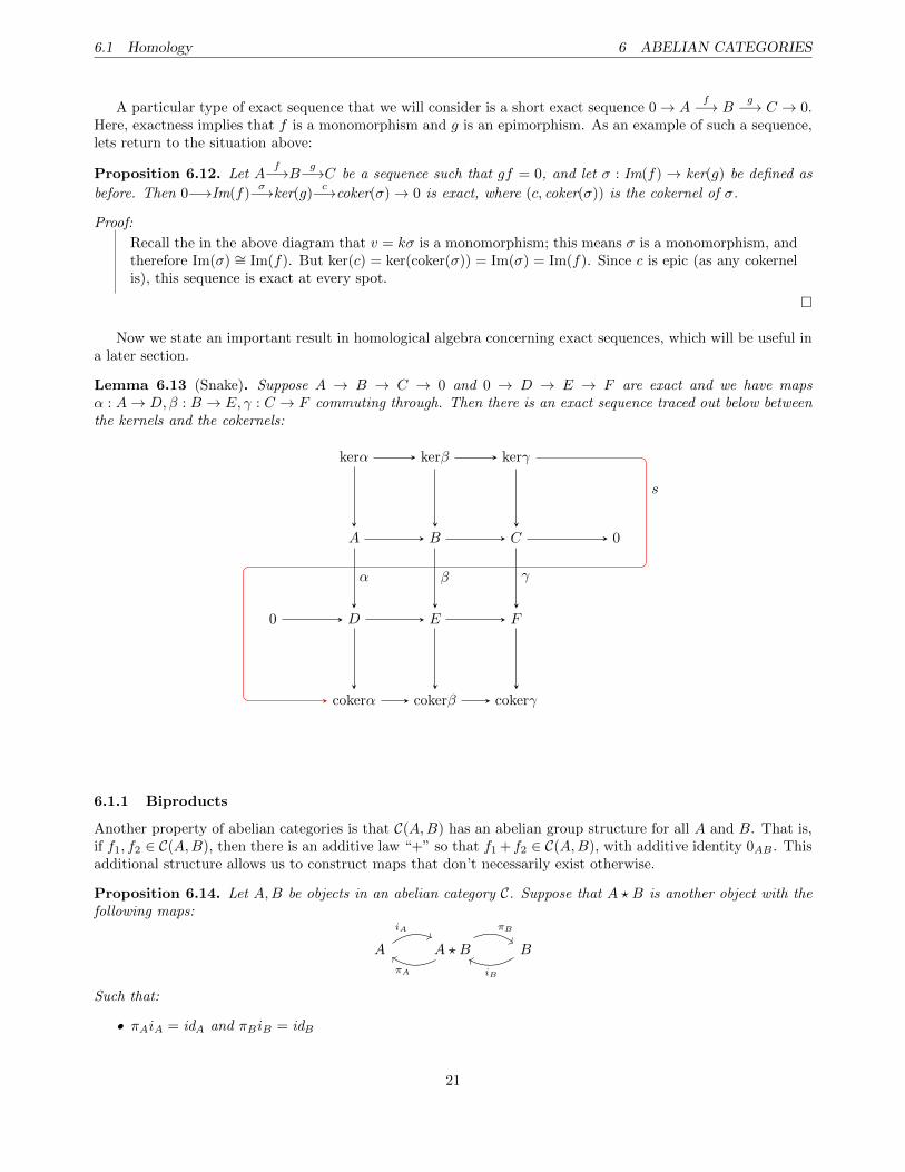
Now we state an important result in homological algebra concerning exact sequences, which will be useful ina later section.
Lemma 6.13 (Snake). Suppose A → B → C → 0 and 0 → D → E → F are exact and we have mapsα : A→ D,β : B → E, γ : C → F commuting through. Then there is an exact sequence traced out below betweenthe kernels and the cokernels:
kerα kerβ kerγ
A B C 0
0 D E F
cokerα cokerβ cokerγ
α β γ
s
6.1.1 Biproducts
Another property of abelian categories is that C(A,B) has an abelian group structure for all A and B. That is,if f1, f2 ∈ C(A,B), then there is an additive law “+” so that f1 + f2 ∈ C(A,B), with additive identity 0AB . Thisadditional structure allows us to construct maps that don’t necessarily exist otherwise.
Proposition 6.14. Let A,B be objects in an abelian category C. Suppose that A ? B is another object with thefollowing maps:
A A ? B B
iA
πA
πB
iB
Such that:
• πAiA = idA and πBiB = idB
21
6.1 Homology 6 ABELIAN CATEGORIES
• πBiA = 0AB and πAiB = 0BA
• iAπA + iBπB = idA?B
Then A ? B is isomorphic to both the product A×B and coproduct AqB.
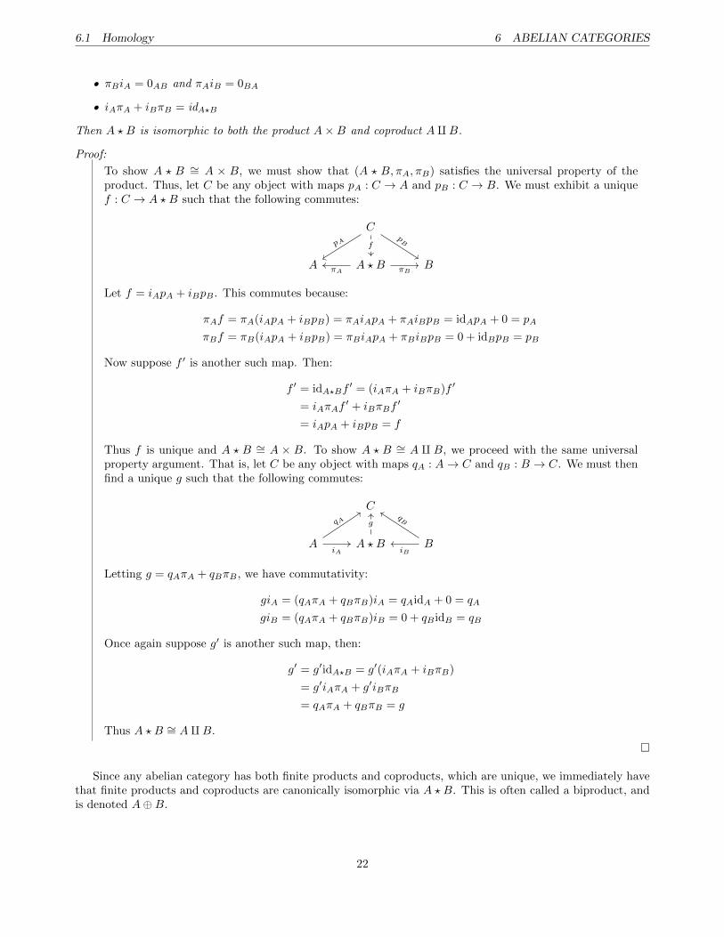
Proof:
To show A ? B ∼= A × B, we must show that (A ? B, πA, πB) satisfies the universal property of theproduct. Thus, let C be any object with maps pA : C → A and pB : C → B. We must exhibit a uniquef : C → A ? B such that the following commutes:
C
A A ? B B
pA fpB
πA πB
Let f = iApA + iBpB . This commutes because:
πAf = πA(iApA + iBpB) = πAiApA + πAiBpB = idApA + 0 = pA
πBf = πB(iApA + iBpB) = πBiApA + πBiBpB = 0 + idBpB = pB
Now suppose f ′ is another such map. Then:
f ′ = idA?Bf′ = (iAπA + iBπB)f ′
= iAπAf′ + iBπBf
′
= iApA + iBpB = f
Thus f is unique and A ? B ∼= A × B. To show A ? B ∼= A q B, we proceed with the same universalproperty argument. That is, let C be any object with maps qA : A→ C and qB : B → C. We must thenfind a unique g such that the following commutes:
C
A A ? B B
qA
iA
g
iB
qB
Letting g = qAπA + qBπB , we have commutativity:
giA = (qAπA + qBπB)iA = qAidA + 0 = qA
giB = (qAπA + qBπB)iB = 0 + qB idB = qB
Once again suppose g′ is another such map, then:
g′ = g′idA?B = g′(iAπA + iBπB)
= g′iAπA + g′iBπB
= qAπA + qBπB = g
Thus A ? B ∼= AqB.
�
Since any abelian category has both finite products and coproducts, which are unique, we immediately havethat finite products and coproducts are canonically isomorphic via A ? B. This is often called a biproduct, andis denoted A⊕B.
22
6.2 Exact Functors 6 ABELIAN CATEGORIES
6.2 Exact Functors
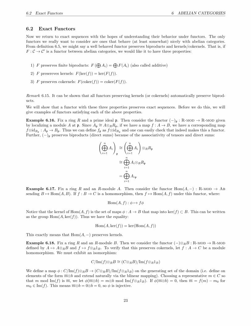
Now we return to exact sequences with the hopes of understanding their behavior under functors. The onlyfunctors we really want to consider are ones that behave (at least somewhat) nicely with abelian categories.From definition 6.5, we might say a well behaved functor preserves biproducts and kernels/cokernels. That is, ifF : C → C′ is a functor between abelian categories, we would like it to have three properties:
1) F preserves finite biproducts: F (⊕Ai) =
⊕F (Ai) (also called additive)
2) F presereves kernels: F (ker(f)) = ker(F (f)).
3) F preserves cokernels: F (coker(f)) = coker(F (f)).
Remark 6.15. It can be shown that all functors preserving kernels (or cokernels) automatically preserve biprod-ucts.
We will show that a functor with these three properties preserves exact sequences. Before we do this, we willgive examples of functors satisfying each of the above properties.
Example 6.16. Fix a ring R and a prime ideal p. Then consider the functor (−)p : R-mod → R-mod givenby localizing a module A at p. Since Ap
∼= A⊗RRp, if we have a map f : A→ B, we have a corresponding mapf⊗idRp
: Ap → Bp. Thus we can define fp as f⊗idRpand one can easily check that indeed makes this a functor.
Further, (−)p preserves biproducts (direct sums) because of the asssociativity of tensors and direct sums:(n⊕i=1
Ai
)p
∼=
(n⊕i=1
Ai
)⊗RRp
∼=n⊕i=1
Ai⊗RRp
=
n⊕i=1
Aip
Example 6.17. Fix a ring R and an R-module A. Then consider the functor Hom(A,−) : R-mod → Absending B 7→ Hom(A,B). If f : B → C is a homomorphism, then f 7→ Hom(A, f) under this functor, where:
Hom(A, f) : φ 7→ fφ
Notice that the kernel of Hom(A, f) is the set of maps φ : A→ B that map into ker(f) ⊂ B. This can be writtenas the group Hom(A, ker(f)). Thus we have the equality:
Hom(A, ker(f)) = ker(Hom(A, f))
This exactly means that Hom(A,−) preserves kernels.
Example 6.18. Fix a ring R and an R-module B. Then we consider the functor (−)⊗RB : R-mod→ R-moddefined by A 7→ A⊗RB and f 7→ f⊗R1B . To verify that this preserves cokernels, let f : A → C be a modulehomomorphism. We must exhibit an isomorphism:
C/Im(f)⊗RB ∼= (C⊗RB)/Im(f⊗R1B)
We define a map φ : C/Im(f)⊗RB → (C⊗RB)/Im(f⊗R1B) on the generating set of the domain (i.e. define onelements of the form m⊗b and extend naturally via the blinear mapping). Choosing a representative m ∈ C sothat m mod Im(f) is m, we let φ(m⊗b) = m⊗b mod Im(f⊗R1B). If φ(m⊗b) = 0, then m = f(m) −m0 form0 ∈ Im(f). This means m⊗b = 0⊗b = 0, so φ is injective.
23
6.2 Exact Functors 6 ABELIAN CATEGORIES
Now consider generating elements of (C⊗RB)/Im(f⊗R1B), which take the form (m⊗b). Notice that we have:
m⊗b = m⊗b+m0⊗b′
for any m0 ∈ Im(f) and b′ ∈ Im(1B) = B, and where m⊗b is a lifting of m⊗b. Letting b′ = b we have:
m⊗b = m⊗b+m0⊗b = (m+m0)⊗b
Therefore the element m⊗b ∈ C/Im(f)⊗RB maps to m⊗b under φ, so we have a surjection and thus anisomorphism. Therefore (−)⊗RB is a functor that preserves cokernels.
We now proceed to relating these three properties of functors on abelian categories to the preservation ofexact sequences.
Theorem 6.19. Let F : C → C′ be an additive functor between two abelian categories. Then the following areequivalent:
1. F preserves exact sequences.
2. F preserves short exact sequences.
3. F preserves kernels and cokernels.
Before we prove this, a quick lemma:
Lemma 6.20. F (0) = 0 for an additive functor F : C → C′ between abelian categories.
Proof:
Notice that A ∈ C is the zero object if and only if C(A,A) ∼= 0 as a groupa. This is equivalent tosaying the identity morphism is the zero morphism on A. Since F is a functor we have F (id0) = idF (0),and since it is also a group homomorphism we also have F (000) = 0F (0)F (0). Since id0 = 000, we haveidF (0) = 0F (0)F (0), and so F (0) is the zero object.
aRecall all hom-sets in an abelian category have a group structure
�
Proof (of Theorem 6.19):
(1) → (3): Let f : A → B be a morphism. Then we have an exact sequence 0 → ker(f)k−→A f−→B.
Since F preserves exact sequences and since F (0) = 0, we have another exact sequence:
0 F (ker(f)) F (A) F (B)F (k) F (f)
Exactness means ker(F (f)) = Im(F (k)). But since F (k) is a monomorphism, its image is isomorphic toF (ker(f)). Thus ker(F (f)) = F (ker(f)) and F preserves kernels. Similarly, we can obtain another exactsequence:
F (A) F (B) F (coker(f)) 0F (f) F (c)
By Proposition 6.7, we have coker(F (f)) = Im(F (c)). As F (c) is an epimorphism, its image is isomor-phic to F (coker(f)). Thus coker(F (f)) = F (coker(f)) and so F preserves cokernels.
(3)→ (2): Let 0→ Af−→ B
g−→ C → 0 be exact. Then by similar reasoning as above we have A ∼= ker(g)and C ∼= coker(f). Applying F gives:
0 F (ker(g)) B F (coker(f)) 0F (f) F (g)
24
6.2 Exact Functors 6 ABELIAN CATEGORIES
Since F preserves kernels and cokernels, which equals:
0 ker(F (g)) B cokerF (f) 0F (f) F (g)
Which is exact.
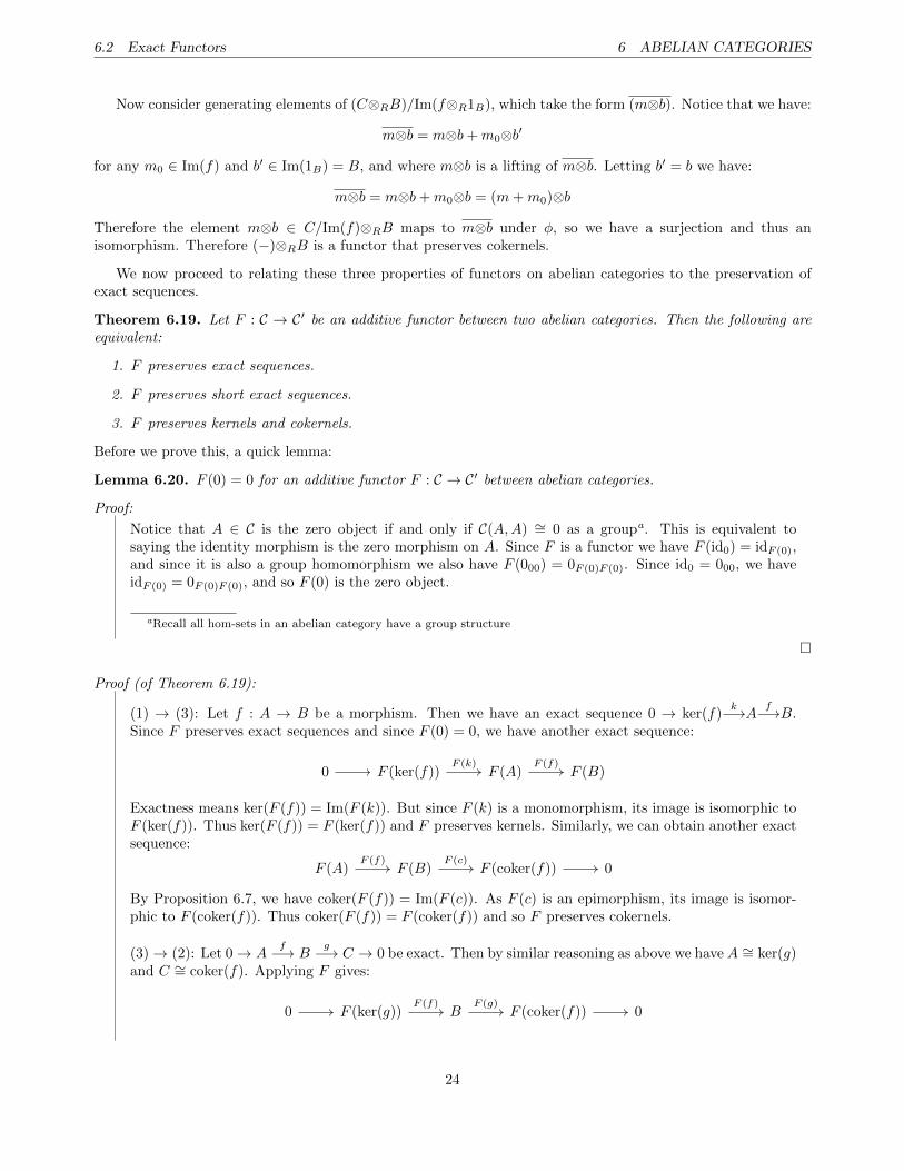
(2) → (1): Let A• be an exact sequence. Then we can factorize any subsequence Ai−1 → Ai → Ai+1
and apply the functor F , resulting in:
0 0 0
F (ker(δi−1)) F (Im(δi))
. . . F (Ai−1) F (Ai) F (Ai+1) . . .
F (Im(δi−1)) F (coker(δi))
0 0 0
qF (δi−1)
u
F (δi)p
v
Since the diagonals were short exact before applying F , they are also short exact after applying F sincewe are assuming (2). This implies that v, q are monic and u, p are epic and that Im(v) = ker(p). Nowwe have:
Im(F (δi−1)) = Im(vu)
= Im(v) (v is epic)
= ker(p)
= ker(qp) (q is monic)
= ker(F (δi))
Thus F (A•) is exact at position i, and therefore everywhere.
�
Now that we see the equivalence of these conditions, we define an exact functor:
Definition 6.21. A functor is called exact if it preserves short exact sequences. If it preserves kernels it is calledleft exact, and if it preserves cokernels it is called right exact.
Corollary 6.22. A left exact functor it preserves monomorphisms, and a right exact functor preserves andepimorphisms.
Proof:
This follows from the preceeding proof of (1)→ (3). That is, letting ker(f) = 0, if F (ker(f)) = F (0) = 0is the kernel of F (f), then it is a monomorphism. Similarly, letting coker(f) = 0, if F (coker(f)) =F (0) = 0 is the cokernel of F (f), then it is an epimorphism.
�
Corollary 6.23. In R-mod, the functor Hom(A,−) is left exact, the functor (−)⊗B is right exact, and thefunctor (−)p is both left and right exact (i.e. exact).
25
6.3 Injective and Projective Objects 6 ABELIAN CATEGORIES
6.3 Injective and Projective Objects
We now generalize to the functors Hom(A,−) and Hom(−, B) in any abelian category. This section will char-acterize what types of objects A and B need to be to make these functors exact. As any hom set in an abeliancategory is an abelian group, these are functors to Ab. If the former maps from a category C, then the lattercan be thought of as mapping from Cop. Below we define how they act on morphisms, so let f : X → Y be amorphism, and let f : Y → X be the corresponding morphism in Cop.
Hom(A, f) : Hom(A,X)→ Hom(A, Y )
φ 7→ fφ
Hom(f,B) : Hom(X,B)→ Hom(Y,B)
φ 7→ φ f
It is not too hard to convince oneself that these are both left exact functors, as we saw in the category of Rmodules. In the case of Hom(A,−), we may apply it to a short exact sequence and obtain:
0 Hom(A,X) Hom(A, Y ) Hom(A,Z) 0Hom(A,f) Hom(A,g)
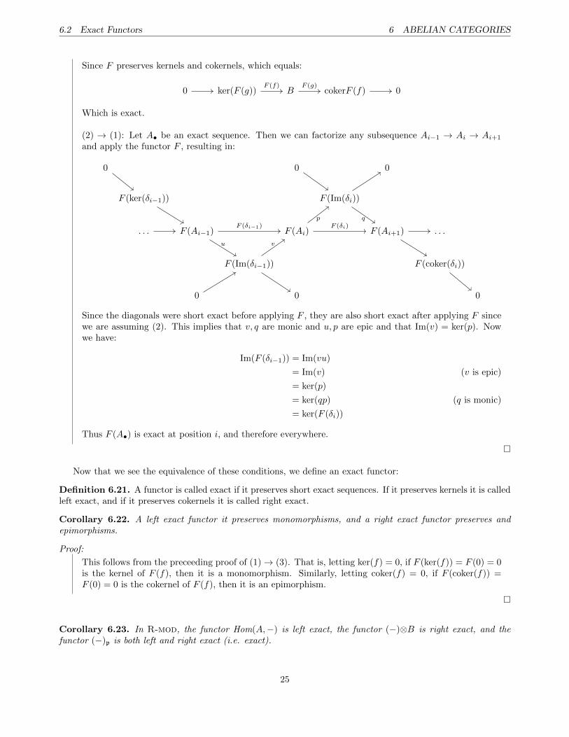
This is not necessarily exact for arbitrary A; however we may easily characterize when it is. Since Hom(A, f) ismonic, we need only check exactness in the middle and that Hom(A, g) is epic. Certainly we have Im(Hom(A, f)) ⊂ker(Hom(A, g)) by the chain condition gf = 0, so let φ ∈ ker(Hom(A, g)). By assumption, gφ = 0AZ , so by theuniversal property of the kernel we have a map φ : A→ kerg. Since kerg ∼= Imf ∼= X, we have φ : A→ X suchthat fφ = φ. Therefore we have exactness at the middle for any A. The only place that this fails to be exactis in the surjectivity of Hom(A, g). Suppose that A has the property that for any ψ ∈ Hom(A,Z), there existsφ ∈ Hom(A,X) so that gφ = ψ. Endowing A with this property for any epimorphism g gives the definition fora projective object:
Definition 6.24. An object P of an abelian category is projective if, for any two objects M,N with mapsf : P → N and g : M → N epic, there is a map h such that the following commutes:
P
M N 0
∃h f
g
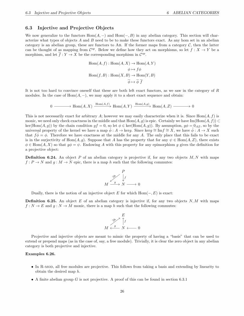
Dually, there is the notion of an injective object E for which Hom(−, E) is exact:
Definition 6.25. An object E of an abelian category is injective if, for any two objects N,M with mapsf : N → E and g : N →M monic, there is a map h such that the following commutes:
E
M N 0
∃h
g
f
Projective and injective objects are meant to mimic the property of having a “basis” that can be used toextend or prepend maps (as in the case of, say, a free module). Trivially, it is clear the zero object in any abeliancategory is both projective and injective.
Examples 6.26.
• In R-mod, all free modules are projective. This follows from taking a basis and extending by linearity toobtain the desired map h.
• A finite abelian group G is not projective. A proof of this can be found in section 6.3.1
26
6.3 Injective and Projective Objects 6 ABELIAN CATEGORIES
Proposition 6.27. Let X be an object in an abelian category. Then:
1. X is projective if and only if Hom(X,−) is exact.
2. Every short exact sequence 0→Mf→ N
g→ X → 0 splits if X is projective.
3. X is injective if and only if Hom(−, X) is exact.
4. Every short exact sequence 0→ Xf→M
g→ N → 0 splits if X is injective.
Proof:
(1): This is by definition of projectivity and the discussion above.(2): We may apply projectivity of X to the identity map 1X ; that is, since g is an epimorphism, we havesome h : X → N so that gh = 1X . This means the sequence splits.(3), (4): Reversing all arrows gives an equivalent proofs as above in Cop.
�
Having an exact sequence split is helpful because, by the Splitting Lemma, we can write the center object asa biproduct of the outer two and thus applying any (additive) functor preserves exactness.
6.3.1 Projective and Injective Modules
The above proposition become stronger in the category R-mod because any module can be written as a quotientof a free module:
Lemma 6.28. Any R-module M is the quotient of a free module.
Proof:
Let F be the module generated by all elements of M . Then there is a module surjection f : F → Minduced by specifying f(ei) = mi for each basis element. Then F/ker(f) ∼= M by the First IsomorphismTheorem.
�
Proposition 6.29. Let X be a module. Then if every short exact sequence 0→Mf→ N
g→ X → 0 splits, then
X is projective. Similarly, if every short exact sequence 0→ Xf→M
g→ N → 0 splits, then X is injective.
Proof:
We will prove the first statement, and the second follows from the same argument in R-modop. ByLemma 6.28, X is a quotient of a free module and therefore we have an exact sequence:
0 L F X 0
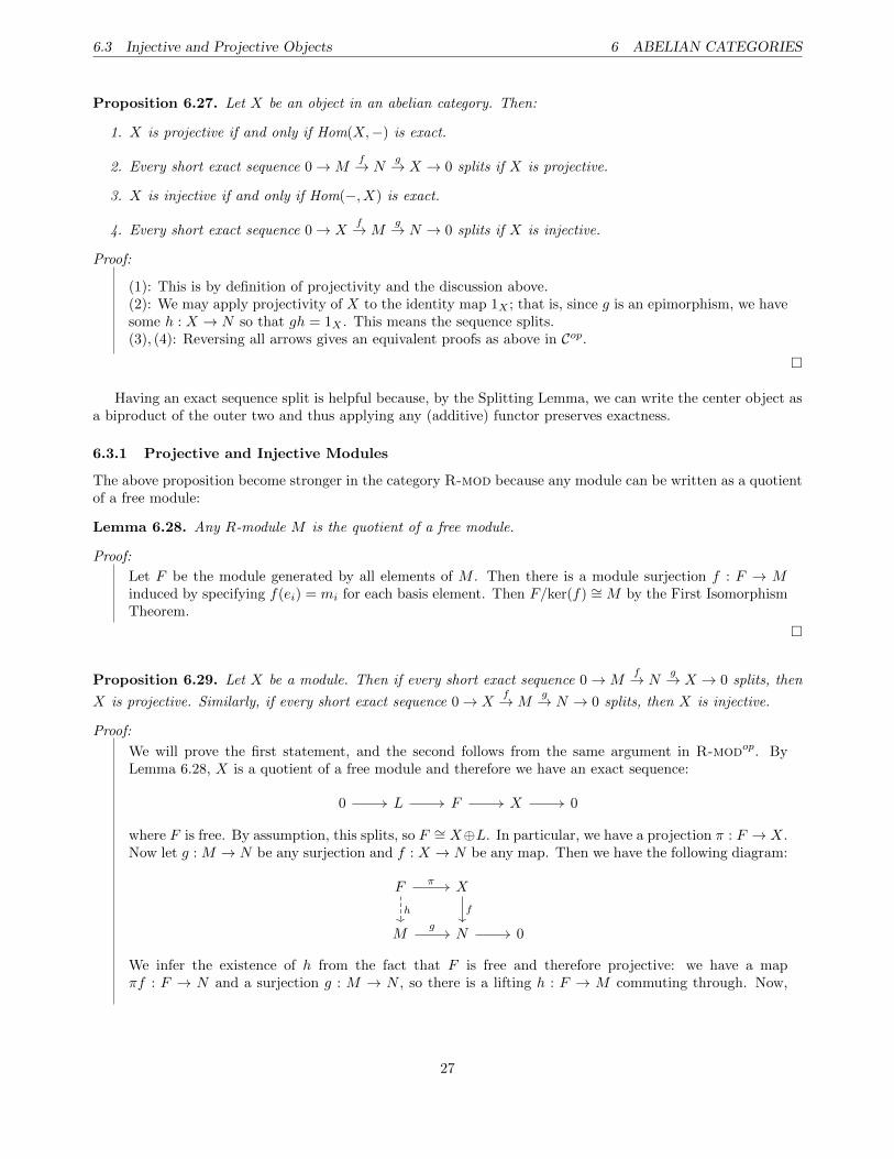
where F is free. By assumption, this splits, so F ∼= X⊕L. In particular, we have a projection π : F → X.Now let g : M → N be any surjection and f : X → N be any map. Then we have the following diagram:
F X
M N 0
π
h f
g
We infer the existence of h from the fact that F is free and therefore projective: we have a mapπf : F → N and a surjection g : M → N , so there is a lifting h : F → M commuting through. Now,
27
6.4 The Chain Complex Category 6 ABELIAN CATEGORIES
since X is a submodule of F , we can restrict h to X and obtain hX : X → M . This shows that X isprojective.
�
Theorem 6.30. A module X over a PID is projective if and only if it is free.
Proof:
One direction has been shown: every free module is projective. Conversely, if X is projective, then itis a summand of a free module (by above) and is therefore a submodule of a free module. Since everysubmodule of a free module in a PID is also free, we have that X is free.
�
Corollary 6.31. A finite abelian group G is not projective as a Z module.
Proof:
G cannot be a free module because all elements have finite order, and thus cannot be part of a basis.As Z is a PID, this also means G is not projective by Theorem 6.30
�
6.4 The Chain Complex Category
We now revisit the idea of chain complexes to give them their own categorical structure. In this section we willdefine the category of chain and cochain complexes for an abelian category. It will conclude with the Zig-ZagLemma, which will be important for future sections.
Definition 6.32. Let C be an abelian category. Then define the category of chain complexes Ch(C) by:
• Objects: chain complexes A• (of any degree) with objects in C.
• A morphism f• : A• → B• is a collection fi : Ai → Bi so that the following commutes for all i:
Ai Ai−1
Bi Bi−1
αi
fi fi−1
βi
The cochain category is the category of chain complexes on Cop.
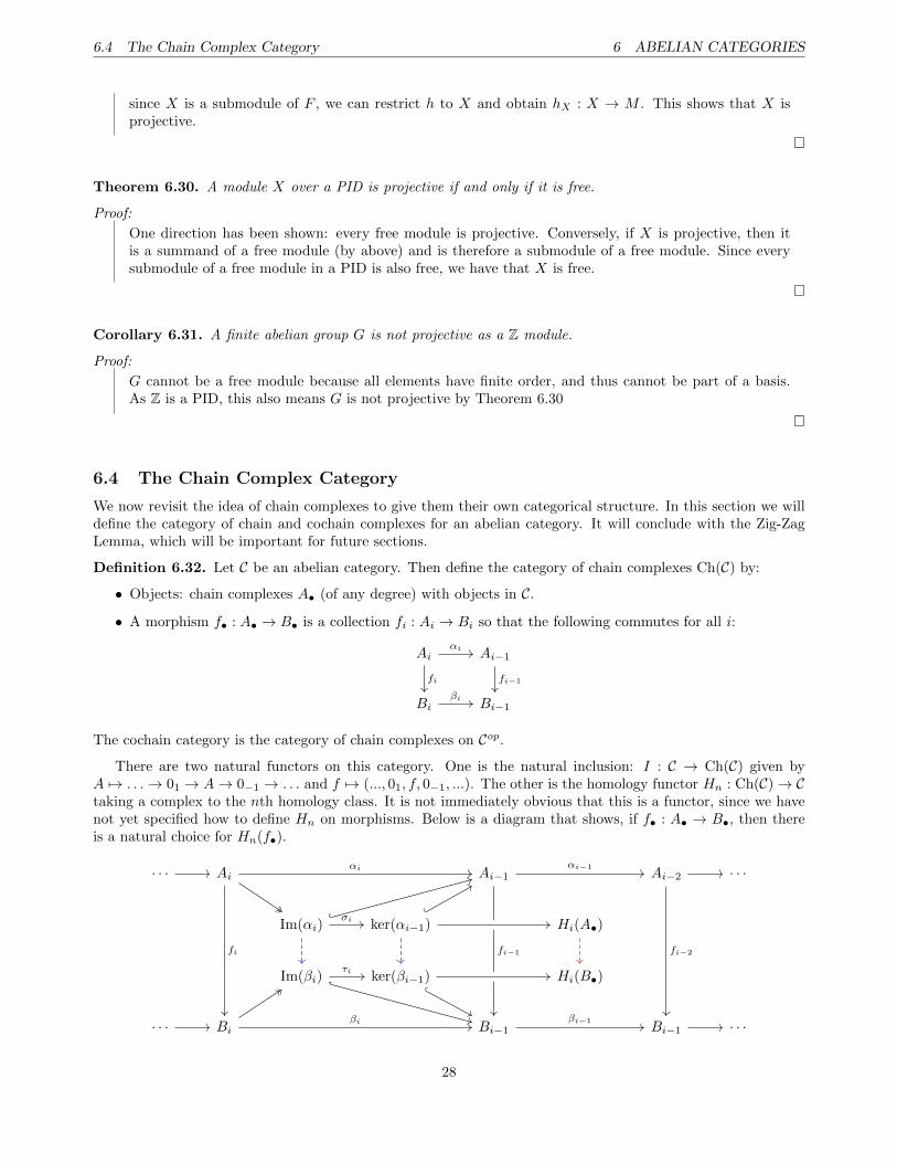
There are two natural functors on this category. One is the natural inclusion: I : C → Ch(C) given byA 7→ . . .→ 01 → A→ 0−1 → . . . and f 7→ (..., 01, f, 0−1, ...). The other is the homology functor Hn : Ch(C)→ Ctaking a complex to the nth homology class. It is not immediately obvious that this is a functor, since we havenot yet specified how to define Hn on morphisms. Below is a diagram that shows, if f• : A• → B•, then thereis a natural choice for Hn(f•).
· · · Ai Ai−1 Ai−2 · · ·
Im(αi) ker(αi−1) Hi(A•)
Im(βi) ker(βi−1) Hi(B•)
· · · Bi Bi−1 Bi−1 · · ·
αi
fi
αi−1
fi−1 fi−2
σi
τi
βi βi−1
28
6.4 The Chain Complex Category 6 ABELIAN CATEGORIES
The blue arrows are inherited maps from the universal property of the kernel, and the red arrow is inducedby the blue arrows because the middle two rows are exact. We can now define Hi(f•) : Hi(A•)→ Hi(B•) to bethe red arrow.
Definition 6.33. A map f• of chain complexes is a quasi-isomorphism if Hi(f•) is an isomorphism for all i.
The quasi-isomorphisms of chain complexes identify complexes that are in some sense similar (i.e. have thesame homology). These are not isomorphisms for many reasons; one of which is that being quasi-isomorphic isnot symmetric.
Theorem 6.34. For an abelian category C, the chain complex category is also abelian.
In particular, we have notions of biproducts, kernels, cokernels and exact sequences in Ch(C). These will notplay a very large role in the discussion to come, so we won’t prove this theorem here. One object that we willuse is the short exact sequence of chain complexes:
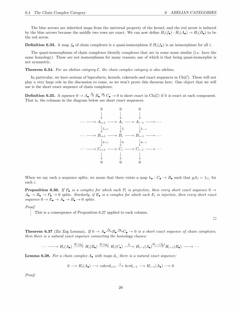
Definition 6.35. A squence 0→ A•f•→ B•
g•→ C• → 0 is short exact in Ch(C) if it is exact at each component.That is, the columns in the diagram below are short exact sequences.
0 0 0
· · · Ai+1 Ai Ai−1 · · ·
· · · Bi+1 Bi Bi−1 · · ·
· · · Ci+1 Ci Ci−1 · · ·
0 0 0
fi+1 fi fi−1
gi+1 gi gi−1
When we say such a sequence splits, we mean that there exists a map h• : C• → B• such that gihi = 1Ci foreach i.
Proposition 6.36. If P• is a complex for which each Pi is projective, then every short exact sequence 0 →A• → B• → P• → 0 splits. Similarly, if E• is a complex for which each Ei is injective, then every short exactsequence 0→ E• → A• → B• → 0 splits.
Proof:
This is a consequence of Proposition 6.27 applied to each column.
�
Theorem 6.37 (Ziz Zag Lemma). If 0 → A•f•−→B•
g•−→C• → 0 is a short exact sequence of chain complexes,then there is a natural exact sequence connecting the homology classes:
· · · Hi(A•) Hi(B•) Hi(C•) Hi−1(A•) Hi−1(B•) · · ·Hi(f•) Hi(g•) δi Hi−1(f•)
Lemma 6.38. For a chain complex A• with maps di, there is a natural exact sequence:
0 Hi(A•) cokerdi+1 kerdi−1 Hi−1(A•) 0ζ
Proof:
29
6.5 Homological dimension 6 ABELIAN CATEGORIES
See [3].
�
Proof Proof (Of Theorem 6.37):
This will be a double application of the Snake Lemma, and is a Proof due to [3]. We first have for everyi a pair of exact sequences:
0 Ai Bi Ci 0
0 Ai−1 Bi−2 Ci−1 0
fi
dAi
gi
dBi dCifi−1 gi−1
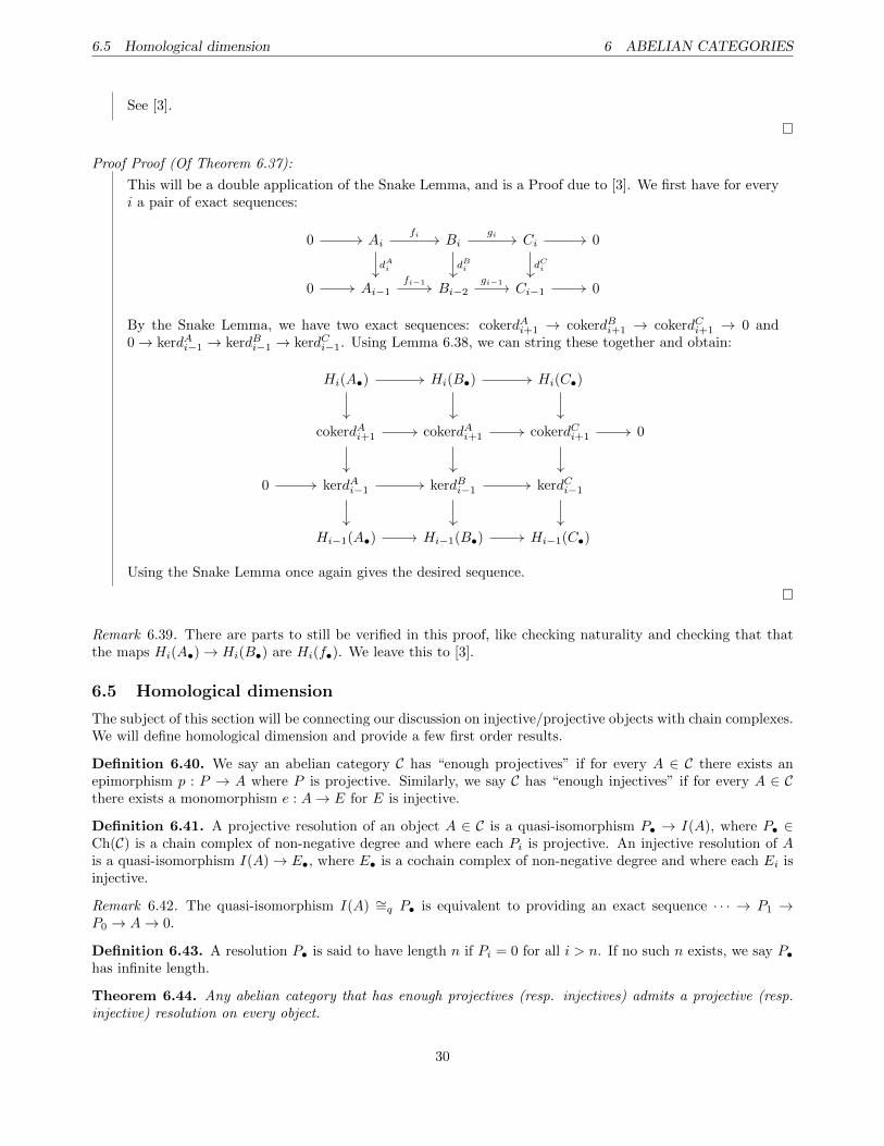
By the Snake Lemma, we have two exact sequences: cokerdAi+1 → cokerdBi+1 → cokerdCi+1 → 0 and0→ kerdAi−1 → kerdBi−1 → kerdCi−1. Using Lemma 6.38, we can string these together and obtain:
Hi(A•) Hi(B•) Hi(C•)
cokerdAi+1 cokerdAi+1 cokerdCi+1 0
0 kerdAi−1 kerdBi−1 kerdCi−1
Hi−1(A•) Hi−1(B•) Hi−1(C•)
Using the Snake Lemma once again gives the desired sequence.
�
Remark 6.39. There are parts to still be verified in this proof, like checking naturality and checking that thatthe maps Hi(A•)→ Hi(B•) are Hi(f•). We leave this to [3].
6.5 Homological dimension
The subject of this section will be connecting our discussion on injective/projective objects with chain complexes.We will define homological dimension and provide a few first order results.
Definition 6.40. We say an abelian category C has “enough projectives” if for every A ∈ C there exists anepimorphism p : P → A where P is projective. Similarly, we say C has “enough injectives” if for every A ∈ Cthere exists a monomorphism e : A→ E for E is injective.
Definition 6.41. A projective resolution of an object A ∈ C is a quasi-isomorphism P• → I(A), where P• ∈Ch(C) is a chain complex of non-negative degree and where each Pi is projective. An injective resolution of Ais a quasi-isomorphism I(A)→ E•, where E• is a cochain complex of non-negative degree and where each Ei isinjective.
Remark 6.42. The quasi-isomorphism I(A) ∼=q P• is equivalent to providing an exact sequence · · · → P1 →P0 → A→ 0.
Definition 6.43. A resolution P• is said to have length n if Pi = 0 for all i > n. If no such n exists, we say P•has infinite length.
Theorem 6.44. Any abelian category that has enough projectives (resp. injectives) admits a projective (resp.injective) resolution on every object.
30
6.5 Homological dimension 6 ABELIAN CATEGORIES
Proof:
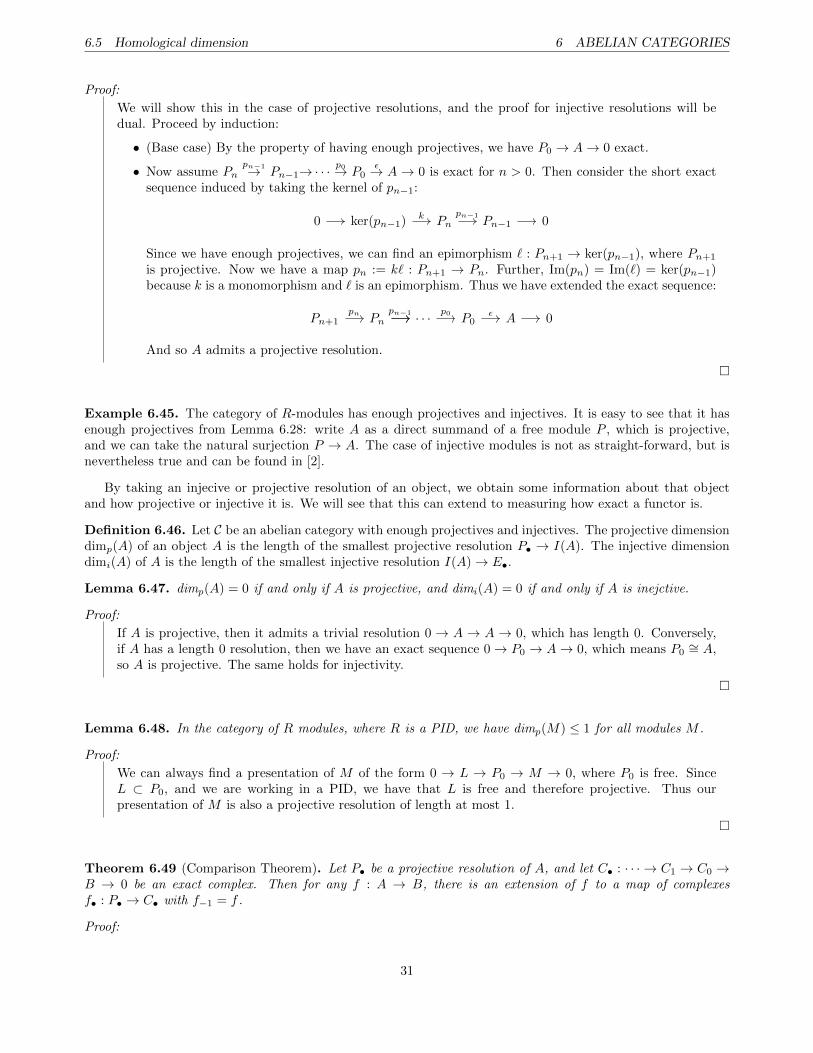
We will show this in the case of projective resolutions, and the proof for injective resolutions will bedual. Proceed by induction:
• (Base case) By the property of having enough projectives, we have P0 → A→ 0 exact.
• Now assume Pnpn−1→ Pn−1→· · ·
p0→ P0ε→ A → 0 is exact for n > 0. Then consider the short exact
sequence induced by taking the kernel of pn−1:
0 ker(pn−1) Pn Pn−1 0k pn−1
Since we have enough projectives, we can find an epimorphism ` : Pn+1 → ker(pn−1), where Pn+1
is projective. Now we have a map pn := k` : Pn+1 → Pn. Further, Im(pn) = Im(`) = ker(pn−1)because k is a monomorphism and ` is an epimorphism. Thus we have extended the exact sequence:
Pn+1 Pn · · · P0 A 0pn pn−1 p0 ε
And so A admits a projective resolution.
�
Example 6.45. The category of R-modules has enough projectives and injectives. It is easy to see that it hasenough projectives from Lemma 6.28: write A as a direct summand of a free module P , which is projective,and we can take the natural surjection P → A. The case of injective modules is not as straight-forward, but isnevertheless true and can be found in [2].
By taking an injecive or projective resolution of an object, we obtain some information about that objectand how projective or injective it is. We will see that this can extend to measuring how exact a functor is.
Definition 6.46. Let C be an abelian category with enough projectives and injectives. The projective dimensiondimp(A) of an object A is the length of the smallest projective resolution P• → I(A). The injective dimensiondimi(A) of A is the length of the smallest injective resolution I(A)→ E•.
Lemma 6.47. dimp(A) = 0 if and only if A is projective, and dimi(A) = 0 if and only if A is inejctive.
Proof:
If A is projective, then it admits a trivial resolution 0 → A → A → 0, which has length 0. Conversely,if A has a length 0 resolution, then we have an exact sequence 0→ P0 → A→ 0, which means P0
∼= A,so A is projective. The same holds for injectivity.
�
Lemma 6.48. In the category of R modules, where R is a PID, we have dimp(M) ≤ 1 for all modules M .
Proof:
We can always find a presentation of M of the form 0 → L → P0 → M → 0, where P0 is free. SinceL ⊂ P0, and we are working in a PID, we have that L is free and therefore projective. Thus ourpresentation of M is also a projective resolution of length at most 1.
�
Theorem 6.49 (Comparison Theorem). Let P• be a projective resolution of A, and let C• : · · · → C1 → C0 →B → 0 be an exact complex. Then for any f : A → B, there is an extension of f to a map of complexesf• : P• → C• with f−1 = f .
Proof:
31
6.6 Derived Functors 6 ABELIAN CATEGORIES
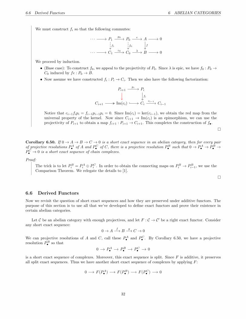
We must construct fi so that the following commutes:
· · · P1 P0 A 0
· · · C1 C0 B 0
f1
p0 ε
f0 f
c0 λ
We proceed by induction.
• (Base case): To construct f0, we appeal to the projectivity of P0. Since λ is epic, we have f0 : P0 →C0 induced by fε : P0 → B.
• Now assume we have constructed fi : Pi → Ci. Then we also have the following factorization:
Pi+1 Pi
Ci+1 Im(ci) Ci Ci−1
pi
fi
ci−1
Notice that ci−1fipi = fi−1pi−1pi = 0. Since Im(ci) = ker(ci−1), we obtain the red map from theuniversal property of the kernel. Now since Ci+1 → Im(ci) is an epimorphism, we can use theprojectivity of Pi+1 to obtain a map fi+1 : Pi+1 → Ci+1. This completes the construction of f•.
�
Corollary 6.50. If 0→ A→ B → C → 0 is a short exact sequence in an abelian category, then for every pairof projective resolutions PA• of A and PC• of C, there is a projective resolution PB• such that 0→ PA• → PB• →PC• → 0 is a short exact sequence of chain complexes.
Proof:
The trick is to let PBi = PAi ⊕ PCi . In order to obtain the connecting maps on PBi → PBi−1, we use theComparison Theorem. We relegate the details to [1].
�
6.6 Derived Functors
Now we revisit the question of short exact sequences and how they are preserved under additive functors. Thepurpose of this section is to use all that we’ve developed to define exact functors and prove their existence incertain abelian categories.
Let C be an abelian category with enough projectives, and let F : C → C′ be a right exact functor. Considerany short exact sequence:
0→ Af−→ B
g−→ C → 0
We can projective resolutions of A and C, call these PA• and PC• . By Corollary 6.50, we have a projectiveresolution PB• so that
0 PA• PB• PC• 0
is a short exact sequence of complexes. Moreover, this exact sequence is split. Since F is additive, it preservesall split exact sequences. Thus we have another short exact sequence of complexes by applying F :
0 F (PA• ) F (PB• ) F (PC• ) 0
32
6.6 Derived Functors 6 ABELIAN CATEGORIES
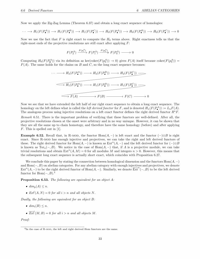
Now we apply the Zig-Zag Lemma (Theorem 6.37) and obtain a long exact sequence of homologies:
· · · H1(F (PA• )) H1(F (PB• )) H1(F (PC• )) H0(F (PA• )) H0(F (PB• )) H0(F (PC• )) 0
Now we use the fact that F is right exact to compute the H0 terms above. Right exactness tells us that theright-most ends of the projective resolutions are still exact after applying F :
F (PA2 ) F (PA1 ) F (PA0 ) 0F (pA1 ) F (pA0 )
Computing H0(F (PA• )) via its definition as ker(coker(F (pA0 )) → 0) gives F (A) itself because coker(F (pA0 )) =F (A). The same holds for the chains on B and C, so the long exact sequence becomes:
· · · H2(F (PA• )) H2(F (PB• )) H2(F (PC• ))
H1(F (PA• )) H1(F (PB• )) H1(F (PC• ))
F (A) F (B) F (C) 0
Now we see that we have extended the left half of our right exact sequence to obtain a long exact sequence. Thehomology on the left defines what is called the left derived functor for F , and is denoted Hn(F (PA• )) := LnF (A).The analogous process using injective resolutions on a left exact functor defines the right derived functor RnF .
Remark 6.51. There is the important problem of verifying that these functors are well-defined. After all, theprojective resolutions chosen at the onset were arbitrary and in no way uniuque. However, it can be shown thatthey are all the same up to chain homotopy, and therefore have the same homology (before) and after applyingF . This is spelled out in [1].
Example 6.52. Recall that, in R-mod, the functor Hom(A,−) is left exact and the functor (−)⊗B is rightexact. Since R-mod has enough injective and projectives, we can take the right and left derived functors ofthese. The right derived functor for Hom(A,−) is known as Extn(A,−) and the left derived functor for (−)⊗Bis known as Torn(−, B). We notice in the case of Hom(A,−) that, if A is a projective module, we can taketrivial resolutions and obtain Extn(A,M) = 0 for all modules M and integers n > 0. However, this means thatthe subsequent long exact sequence is actually short exact, which coincides with Proposition 6.27.
We conclude this paper by stating the connection between homological dimension and the functors Hom(A,−)and Hom(−, B) on abelian categories. For any abelian category with enough injectives and projectives, we denoteExtn(A,−) to be the right derived functor of Hom(A,−). Similarly, we denote Ext
n(−, B) to be the left derived
functor for Hom(−, B).4
Proposition 6.53. The following are equivalent for an object A:
• dimp(A) ≤ n.
• Exti(A,N) = 0 for all i > n and all objects N .
Dually, the following are equivalent for an object B:
• dimi(B) ≤ n.
• Exti(M,B) = 0 for all i > n and all objects M .
Proof:
4In the case of R-mod, the left and right derived Hom functors are the same.
33
6.6 Derived Functors 6 ABELIAN CATEGORIES
See [2].
�
34
7 TRIANGULATED AND DERIVED CATEGORIES
7 Triangulated and Derived Categories
TODO
35
References
[1] Swanson, Irena. Homological Algebra. Reed College, 2010.http://people.reed.edu/∼iswanson/homologicalalgebra.pdf
[2] Ash, Robert B. Abstract Algebra: The Basic Graduate Year. The University of Illinois at Urbana Champaign.http://www.math.uiuc.edu/∼r-ash/Algebra.html
[3] Gim, Geunho. Homological Algebra - Lecture Notes. Math 212, University of California Los Angeles. 2014.http://www.math.ucla.edu/∼ggim/S14-212lecturenote.pdf