Non-planar lifting-line theory for fixed and deformable geometries

NON-PLANAR LIFTING-LINE THEORY FOR FIXED AND DEFORMABLE GEOMETRIES

A Thesis by

Aaron Douglas Kuenn

Bachelor of Arts, Bethany College, 2009

Submitted to the Department of Aerospace Engineering and the faculty of the Graduate School of

Wichita State University in partial fulfillment of

the requirements for the degree of Master of Science

August 2013

© Copyright 2013 by Aaron Douglas Kuenn

All Rights Reserved

iii

NON-PLANAR LIFTING-LINE THEORY FOR FIXED AND DEFORMABLE GEOMETRIES

The following faculty members have examined the final copy of this thesis for form and content, and recommend that it be accepted in partial fulfillment of the requirement for the degree of Master of Science, with a major in Aerospace Engineering. Linda Kliment, Committee Chair Kamran Rokhsaz, Committee Member Ikram Ahmed, Committee Member

iv

ABSTRACT

In this thesis, the lifting-line approximation of a flat, unswept wing, originally attributed

to Prandtl, is investigated. The original formulation for a flat wing is examined in detail. The

governing integro-differential equation is developed from its components. The optimum and

general solutions to the original formulation are presented and discussed.

An expanded formulation is presented, which includes the effect of the wake of non-

planar wings. The self-induced velocities of the bound vortex on the wing are assumed to be

small for practical cases and not included in the model. The case of simple dihedral is

considered and the general formulation is simplified to better illustrate the effect of the geometry

on the governing equation. For the simplified dihedral case, the optimal solution remains the

same as for a flat wing.

A simplified finite element model is also included, which accounts for the bending due to

the force generated by the bound vortex. This finite element model is combined with the non-

planar lifting-line equation to create a static aeroelastic model for a wing. The solution of this

problem is iterative, but converges quickly. Lift coefficient and span efficiency factor are

provided for a set of wing geometries for cases of dihedral and wing bending, and the trends are

examined compared to flat wings. Additionally, the resulting geometries after deformation of

the wing are presented and the effect of circulation distribution on the resulting shape is

discussed.

v

TABLE OF CONTENTS

Chapter Page

1. INTRODUCTION ...........................................................................................................1

2. CLASSICAL LIFTING LINE THEORY ........................................................................6

2.1 Formulation .......................................................................................................6 2.2 Solutions to the Traditional Formulation ..........................................................10

2.2.1 Elliptic Lift Distribution .................................................................11 2.2.2 General Lift Distribution.................................................................14

3. PRESENT FORMULATION ..........................................................................................19

3.1 General Formulation .........................................................................................19 3.2 Specific Formulations .......................................................................................23

3.2.1 Dihedral...........................................................................................23 3.2.2 Deformable Wing............................................................................25

3.3 Solution to Non-Planar Formulations ...............................................................28 4. RESULTS AND DISCUSSION ......................................................................................31

4.1 Convergence Analysis ......................................................................................31 4.1.1 Number of Panels ............................................................................31 4.1.2 Numerical Integration Subdivisions ...............................................37

4.2 Wing with Dihedral...........................................................................................37 4.2.1 Effect of Aspect Ratio .....................................................................37 4.2.2 Effect of Dihedral on an Elliptically Loaded Wing ........................42 4.2.3 Effect of Dihedral on Twist ............................................................45 4.2.4 Effect of Dihedral on Taper ............................................................54

4.3 Deformable Wing..............................................................................................56 4.3.1 Deflection ........................................................................................58 4.3.2 Effects on Lift Coefficient and Spanwise Efficiency Factor ..........69

5. CONCLUSION ................................................................................................................76

REFERENCES ............................................................................................................................79

APPENDIX: Non-Planar Lifting Line Code ...............................................................................82

vi

LIST OF TABLES

Table Page

4.1 Effect of Dihedral Angle on Lift Curve Slope and Spanwise Efficiency Factor for Elliptical Wing .............................................................................................43

4.2 Decrease in Span Efficiency Factor for Wings with Compared to Flat ..........................................................................................................49

4.3 Wing Geometries used in Deformable Wing Investigations ........................................57

vii

LIST OF FIGURES

Figure Page

2.1 Horseshoe Vortex System .............................................................................................6

3.1 Generic Non-Planar Wing with Induced Velocities .....................................................21

3.2 Dihedral Wing with Induced Velocities .......................................................................24

4.1 Convergence of Fourier Coefficients for Rectangular Wing ........................................33

4.2(a) Overview of Circulation Distribution over Rectangular Wing .....................................33

4.2(b) Detail of Differences between Normalized Circulation Distributions over Rectangular Wing .........................................................................................................34

4.3 Convergence of Fourier Coefficients for Linearly Tapered Wing ...............................35

4.4 Circulation Distribution over Linearly Tapered Wing .................................................35

4.5 Convergence of Fourier Coefficients for Rectangular Wing with Linear Washout .....36

4.6 Circulation Distribution over Rectangular Wing with Linear Washout .......................36

4.7 (a) Effect of Aspect Ratio on Lift-Curve Slope of Flat Rectangular Wing ........................39

4.7 (b) Effect of Aspect Ratio on Lift-Curve Slope of Rectangular Wing with 6 Degrees of Dihedral ......................................................................................................39

4.8 (a) Effect of Aspect Ratio on Flat Rectangular Wing ........................................................40

4.8 (b) Effect of Aspect Ratio on Rectangular Wing with 6 Degrees of Dihedral ...................40

4.9 Comparison of Span Efficiency Factor, e, for Wings with Varying Aspect Ratio ..................................................................................................................41

4.10 Comparison of Lift-Curve Slope, CLα, for Wings with Varying Aspect Ratios ...........41

4.11 Effect of Dihedral Angle on Lift-Curve Slope for Elliptical Wing ..............................43

4.12 Effect of Dihedral on Drag Coefficient of Elliptical Wing ..........................................44

4.13 Effect of Angle of Attack, α, on Span Efficiency Factor, e, of a Rectangular Wing with 1 Degree of Washout ..............................................................47

4.14 Effect of Dihedral Angle, , on Span Efficiency Factor, e, for Wings at CL = 0.1..........................................................................................................47

viii

LIST OF FIGURES (continued)

Figure Page



4.17 (a) Normalized Spanwise Circulation Distribution for Wings with at ......................................................................................................51

4.17 (b) Normalized Spanwise Circulation Distribution for Wings with at ....................................................................................................51

4.18 (a) Spanwise Circulation Distribution for Wings with at ......................52

4.18 (b) Spanwise Circulation Distribution for Wings with at ....................52

4.19 (a) Normalized Spanwise Circulation Distribution for Wings with at ......................................................................................................53

4.19 (b) Normalized Spanwise Circulation Distribution for Wings with at ....................................................................................................53

4.20 Effect of Dihedral Angle on Lift-Curve Slope of Untwisted, Tapered Wings .............55

4.21 Effect of Dihedral Angle on Span Efficiency Factor of Untwisted, Tapered Wings ...........................................................................................55

4.22 Normalized Deflection of Rectangular Wing with S = 150 ft2 and EI = 1.5x106 at q = 50 psf with Varying Aspect Ratios ...............................................58

4.23 Deflection of an Elliptical Wing with EI = 0.15x106 lbf-ft2 .........................................59

4.24 Angle of Local Normal to Vertical for an Elliptical Wing with EI=0.15x106 lbf-ft2 .....................................................................................60

4.25 Deviations from Elliptical Wing Deflection at CL = 0.25 for Wings with EI = 0.15x106 lbf-ft2 ..................................................................................61



ix


Figure Page

4.28 Wing Deflection Angle Deviation from Elliptical Wing Deflection at CL = 0.25 for Wings with EI = 0.15x106 lbf-ft2 ......................................63



4.31 Spanwise Circulation Distribution at CL = 0.70 for Wings with EI = 0.15x106 lbf-ft2 .............................................................................................64

4.32 Normalized Spanwise Circulation Distribution at CL = 0.70 for Wings with EI = 0.15x106 lbf-ft2 ..................................................................................65

4.33 Deflection of Elliptical Wing at CL = 0.50 with Constant and Linearly Tapered Stiffness .....................................................................................66

4.34 Increase in Elliptical Wing Deflection from Constant EI = 0.15x106 lbf-ft2 at CL = 0.5 for Linearly Tapered Stiffness ..................................67

4.35 Deviations from Elliptical Wing Deflection at CL = 0.5 for Wings with Linearly Tapered Stiffness with Root EI = 0.15x106 lbf-ft2 .................................68

4.36 Wing Deflection Angle Deviation from Elliptical Wing Deflection at CL = 0.5 for Wings with Linearly Tapered Stiffness with Root EI = 0.15x106 lbf-ft2 ...............68

4.37 (a) Lift Coefficient for Deformable Elliptical Wing with Root EI = 0.15x106 lbf-ft2 .......70

4.37 (b) Span Efficiency Factor for Deformable Elliptical Wing with Root EI = 0.15x106 lbf-ft2 ..........................................................................70

4.38 (a) Decrease in Lift Coefficient Due to Wing Deflection for Constant EI = 0.15x106 lbf-ft2 ................................................................................71

4.38 (b) Decrease in Lift Coefficient Due to Wing Deflection for 25% Linearly-Tapered Stiffness with Root EI = 0.15x106 lbf-ft2 .........................................72

4.38 (c) Decrease in Lift Coefficient Due to Wing Deflection for 50% Linearly-Tapered Stiffness with Root EI = 0.15x106 lbf-ft2 .........................................72

4.39 (a) Decrease in Span Efficiency Factor Due to Wing Deflection for Constant EI = 0.15x106 lbf-ft2 ................................................................................74

x


Figure Page

4.39 (b) Decrease in Span Efficiency Factor Due to Wing Deflection for 25% Linearly-Tapered Stiffness with Root EI = 0.15x106 lbf-ft2 .........................................74

4.39 (c) Decrease in Span Efficiency Factor Due to Wing Deflection for 50% Linearly-Tapered Stiffness with Root EI = 0.15x106 lbf-ft2 .........................................75

xi

NOMENCLATURE

a0 lift-curve slope

An Fourier coefficients

AR aspect ratio

b wing span

c wing chord

Cr wing root chord

Ct wing tip chord

Cl 2-dimensional lift coefficient

CL lift coefficient

CN wing normal force coefficient

wing normal force coefficient not generating lift

induced drag coefficient

Di induced drag

e spanwise efficiency factor

F finite element force vector

Fn wing normal force

element of the finite element force vector

h radial distance from a vortex

Ke, KE finite element stiffness matrix

finite element sub matrix

lift per unit span

finite element beam length

xii

NOMENCLATURE (continued)

M finite element moment vector

element of the finite element moment vector

local wing normal direction

p finite element panel end points

S wing area

s arc length

freestream velocity

w downwash

X finite element deflection vector

x, y, z Cartesian coordinates

geometric angle of attack

effective angle of attack

induced angle of attack

wing zero-lift angle of attack

angle between vortex radius and y-direction

vortex strength

induced drag factor

transformation polar coordinates and finite element beam deflection angle in Chapter 3

angle between wing normal and z-direction

air density

lift-curve slope parameter

xiii

NOMENCLATURE (continued)

effective twist angle

1

CHAPTER 1

INTRODUCTION

Efficiency of aircraft has been a primary concern of engineers since the earliest days of

flight. Tools have been developed to analyze large sets of potential geometries for their

efficiency. However, with the advent of airframes taking advantage of aeroelastic properties, it

is important to have tools that can provide information on the behavior of preliminary designs

when lifting surfaces are not flat.

The first formulation of the lifting-line approximation was derived by Prandtl in the mid-

to late-1910s in Germany, published by NACA in the 1920s.1 The original formulation replaced

the wing with an infinite number of horseshoe vortices of undetermined strength. Prandtl found

that an elliptical circulation distribution provided an appropriate solution to the resulting integro-

differential equation, but the equation was not immediately solved for the most general case of

an arbitrary planform.

For unswept wings, Munk2 addressed the minimum induced drag. He showed that

minimum induced drag for a flat wing occurs when the downwash is constant along its span.

This holds true for systems of wings at the same station in the flow direction, and also for

unswept wings at any station in the flow-direction as well, i.e. wings of planes flying in

formation. Munk generalized even further by considering unswept, non-planar wings. He

showed that for these wings, the minimum induced drag occurred when the normal wash, i.e. the

induced velocity normal to the wing, was constant along the span. While an important

advancement, Munk2 did not provide a method with which to determine the planform shape that

produced the induced velocities required to achieve the minimum drag.

2

Shortly after Prandtl’s work was published, Glauert3 proposed a solution to the general

case. Glauert showed that a Fourier sine series could represent the circulation distribution over

the wing and since a Fourier series can represent any continuous function on a closed interval,

this form allowed for the representation of any distribution over the wing. By selecting a finite

number of control points along the wing and requiring the lifting-line equation to be satisfied at

each point, a system of linear equations could be formed, to solve for the unknown Fourier

coefficients. These coefficients were obtained analytically. The collocation method is often

presented in textbooks4,5 as an instructional method to help students understand the

approximation. While popular, the collocation method may not capture sudden changes in

circulation, as due to ailerons or flaps, unless the control points are located in the correct

locations.6

Other solution methods have been developed as alternatives to or improvements on the

collocation method. Methods developed that provide approximate solutions, classified by

Rasmussen and Smith6 as “variational methods,” used weighted integrals to account for the

planform shape and twist.7,8 Another method, used by Karamcheti,9 Lotz,10 and Rasmussen and

Smith,6 represented the twist and chord distributions with Fourier series in addition to the

circulation. Karamchetti and Lotz represented the twist in a conventional Fourier series, and the

chord in terms of its inverse, while Rasmussen and Smith6 represented both with conventional

Fourier series. The benefit seen in Rasmussen and Smith’s work was a more quickly converging

series solution than the traditional collocation method, and a more accurate result when more

terms are used in the series approximation.

Despite the utility of the traditional formulation, it was constrained to unswept, planar

wings. Modifications to the method were made by Weissinger,11 allowing the analysis of swept

3

wings. Weissinger’s method divides the wing into a discrete number of panels, with a horseshoe

vortex on each. These horseshoe vortices were positioned with the bound vortex at the local

quarter-chord, parallel to the leading edge of the wing, with flow tangency enforced at the three-

quarter chord, using Pistolesi’s three-quarter chord theorem.12 Weissinger’s formulation formed

a system of linear equations, similar to Glauert’s.3 This method was developed before the advent

of computers and the solution for 7 control points along the span required about 8 hours of

calculation,11 a significant increase in time over Glauert’s method. This original model was later

modified by Owens,13 who combined it with Prandtl’s non-linear lifting line method, which can

be found in Anderson.4 Owen’s modification agreed favorably with experimental results for lift

and drag and accurately predicted stall location for unswept wings with and without taper and

twist.13

Using the work of Munk2, Cone14 developed a generalization to the original lifting-line

equation which incorporated the effects of the wing being non-planar. During his development,

Cone14 stated that for small to moderate deflection angles, the bound vortex did not contribute a

significant induced velocity on itself and could be ignored for most practical cases. Using

complex change of variables, he solved for the circulation distribution over wings in a family of

circular arc segments, and showed an improvement of span efficiency factor of up to 50% over

that of an elliptical wing of the same span. Cone14 addressed additional geometries of practical

and impractical nature, such as straight winglets at different angles, curved winglets, annular

winglets, and even annular wings. In all cases, wings with non-planar elements showed

increased efficiency over wings with the equivalent projected span.

Additional research concerning non-planar wings has been performed at higher speed

regimes, where many modern transport aircraft fly. One such example is the work by Takahashi

4

and Donovan15, who analyzed various candidate geometries to categorize the most efficient

system using the Treftz plane analysis. This analysis does not use the governing integral

equation developed by Prandtl1 directly, but employs the downwash at a station far downstream

of the wing.9 Takahashi and Donovan15 concentrated on transport category design, which

included a 33 degree sweep and Mach numbers in the transonic regime. The report showed

improvements in efficiency for all non-planar lifting surface configurations, with the greatest

improvements in induced drag resulting from a either a bi-plane configuration or a mono-wing

with boxed winglets.

Nguyen16 focused on the benefits from aeroelastic deformation of a wing on a transport

category aircraft. The structural deformation was considered in the chordwise and normal

directions as well including twisting of the wing. The aerodynamic solution was not achieved

using any derivative of the lifting-line model, but using a computational fluid dynamics code,

which was coupled with the structural analysis. This joint solver was complimented with a

numerical optimizer. The optimized shape proved to be a wing with downward droop toward the

wingtips having a greater efficiency than upward deflected wings, both as compared to an

originally flat baseline wing.

In this thesis, the classical formulation of the problem is discussed in depth in Chapter 2.

The governing integro-differential equation is developed from its components and the optimum

and a generalized solution are presented. Chapter 3 contains the development of the general non-

planar formulation, starting from the classical formulation presented in Chapter 2. The case of

simple dihedral is considered and the general formulation is simplified to better illustrate the

effect the geometry has on the governing equation. A simplified finite element model is

presented to account for wing bending under aerodynamic loads. This model does not account

5

for deformations in torsion. This finite element model is combined with the non-planar lifting-

line equation to create a static aeroelastic model for a wing. The results from the solution of the

non-planar formulations are presented in Chapter 4. The optimum spanwise lift distribution for

wings with dihedral is shown to be elliptical, unchanged from the traditional formulation. Lift

coefficient and span efficiency factor are provided for a set of wing geometries for cases of

dihedral and wing bending, and the trends are examined compared to flat wings. Additionally,

the resulting geometries after deformation of the wing are presented and the effect of circulation

distribution on the resulting shape is discussed.

Finally, Chapter 5 is devoted to the summary of the work, the conclusions drawn, and the

recommendations for further research.

6

CHAPTER 2

CLASSICAL LIFTING LINE THEORY

The classical lifting-line theory is presented in detail. It is assumed that the reader is

familiar with the basic assumptions that are used in the derivation. The theorems used here will

be the Biot-Savart law, Helmholtz’s theorems, the Kutta-Joukowski theorem, and Prandtl’s

theorem. These can be found in sufficient detail in most textbooks (Reference Anderson et al.4).

Elliptical and general lift distributions are provided for the classical lifting line theory.

2.1 Formulation

The following formulation of lifting line theory is originally credited to Ludwig Prandtl.1

However, with its wide applications and usefulness as a teaching tool, the method can be found

in most aerodynamics texts.3,4,5 The formulation presented below follows the formulation found

in Anderson,4 which in turn follows the original reasoning of Prandtl.1

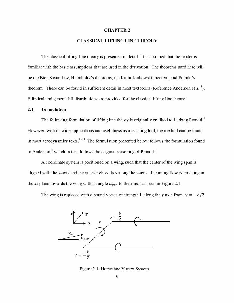
A coordinate system is positioned on a wing, such that the center of the wing span is

aligned with the x-axis and the quarter chord lies along the y-axis. Incoming flow is traveling in

the xz plane towards the wing with an angle to the x-axis as seen in Figure 2.1.

The wing is replaced with a bound vortex of strength along the y-axis from

Figure 2.1: Horseshoe Vortex System

𝛤

=

2

=

2

𝑥

𝑧

𝑉∞ 𝑔𝑒𝑜

7

to . According to the Kutta-Joukowski theorem, this vortex will experience a lifting

force of

𝑉 (2.1)

In order to not violate Helhmoltz’s theorems, the vortex cannot end at the wingtips. Instead, the

vortex will be in the shape of a horseshoe with the filament leaving the wingtip and forming a

two-pronged wake that extends to ∞.

This simple model was one of the first of its form. The deficiency of this simple model

arises with the downwash. The Biot-Savart law shows clearly that the bound vortex does not

induce a velocity upon itself in any direction; however the free vortices from either wingtip

induce a velocity in the negative z-direction across the length of the bound vortex.

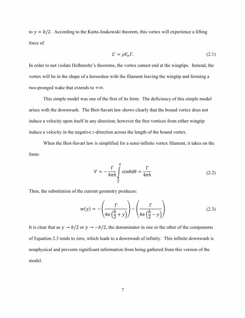
When the Biot-Savart law is simplified for a semi-infinite vortex filament, it takes on the

form:

𝑉

∫

(2.2)

Then, the substitution of the current geometry produces:

( ) (

( )

) (

( )

) (2.3)

It is clear that as or , the denominator in one or the other of the components

of Equation 2.3 tends to zero, which leads to a downwash of infinity. This infinite downwash is

nonphysical and prevents significant information from being gathered from this version of the

model.

8

The solution posed by Prandtl1 is that the wing is not formed by a single horseshoe

vortex, but by a large number superimposed over the wing. By stacking these horseshoe vortices

over one another, the model is accurately represents a continuous distribution over the length.

The bound vortex is then represented by an infinite number of filaments overlaid across

the span of the wing. With an infinite number of horseshoe vortices, each has the infinitesimal

strength, . At any arbitrary location along the bound vortex, an infinitesimal segment can be

isolated. Let this segment be . At this location, the circulation strength is ( ) and the

change over the infinitesimal length, ( ) So as not to violate Helmholtz’s

theorems, if the change in vortex strength over the length is , so must the strength of the

trailing vortex that departs at .

Considering that there is a trailing vortex in each infinitesimal segment, , it is

important to examine the effect that each segment has on an arbitrary location . Using the

Biot-Savart law, it is again evident that there is no effect at due to the bound vortex segment

. The trailing vortex will create a downwash equal to:

(

)

( ) (2.4)

This consideration is then extended to include the induced velocity from the entire wake at the

point . This extension takes the form of an integral from wingtip to wingtip:

( )

∫

(

)

( )

(2.5)

It is helpful at this point to recall that for an airfoil,

(2.6)

9

where is the lift-curve slope of the airfoil and the angle of attack in radians. From inviscid

thin airfoil theory, . Angle of attack, , can be expanded into three parts: geometric

angle of attack, induced angle of attack, and angle at which lift is zero. Therefore, Equation 2.6

can be expressed as:

[ ] (2.7)

The geometric angle of attack can be set by the investigator and the geometry of the wing is

specified at , providing . Since the incoming velocity and downwash are known, the

induced angle of attack at can be determined using Equation 2.8.

( ) ( ( )

𝑉 ) (2.8)

With the assumption that the induced angle of attack is small, since generally 𝑉 , then the

induced angle of attack can be approximated as:

( ) ( )

𝑉 (2.9)

Substituting this into Equation 2.5:

( )

𝑉 ∫

(

)

( )

(2.10)

Lift coefficient may be written as

𝑉

(2.11)

Now, Equation 2.11 and Kutta-Joukowski theorem result in two equivalent definitions for lift per

unit span:

10

𝑉

( ) 𝑉 (2.12)

Equation 2.12 can be rearranged for :

( )

𝑉 ( ) (2.13)

Combining Equation 2.13 with Equation 2.7 provides:

( )

𝑉 ( ) ( ) (2.14)

When Equation 2.9 is substituted for and moved to the other side, Equation 2.14 becomes, as

found in Anderson:4

( ) ( )

𝑉 ( ) ( )

𝑉 ∫

(

)

( )

(2.15)

As Anderson states, “this is the fundamental equation of Prandtl’s lifting-line theory.”4 It is

important to note that the circulation distribution is the only unknown in Equation 2.15.

2.2 Solutions to the Traditional Formulation

With the governing equation assembled, solutions can be presented. After the problem

was derived, Tietjens and Prandtl,17 used trial to find circulation distributions that allowed the

integral to be calculated easily. Coincidentally, a semi-elliptic circulation distribution was found

to produce a simple solution. Only later was this solution found to provide even more important

insight.

Later on, researchers sought formulations that would allow them to input the

characteristics of the wing and solve for the circulation distribution and compare the effect of

various designs. This general method, while useful, is time consuming to calculate by hand.

11

However, with the development and advancement of computers, this method has become the

primary technique to handle the governing equation.

2.2.1 Elliptic Lift Distribution

Suppose the circulation distribution can be expressed as:

( ) √ (

)

(2.16)

where is the circulation at the origin. This equation defines a semi-elliptical distribution of

circulation over the wing. If Equation 2.16 is substituted into Equation 2.1 the result is,

( ) 𝑉 √ (

)

(2.17)

which implies the lift distribution is also elliptical. It can be observed that, as expected,

circulation and lift go to zero at the wingtips.

If Equation 2.17 is used to calculate the downwash over the wing, the derivative is of the

form:

√ (

) (2.18)

When Equation 2.18 is substituted into Equation 2.5, the downwash becomes:

( )

∫

√ (

)

( )

(2.19)

In order to easily evaluate this integral, the following simplification can be made for :

𝑜 (2.20)

12

When this substitution is made to Equation 2.19, with the limits being transformed to and

respectively, the downwash becomes:

( )

(2.21)

It is of value to note that downwash is constant over the entire wing. This will be discussed in

further detail later. Retaining the assumption of small angles:

( ) ( )

𝑉

𝑉 (2.22)

If Equation 2.17 is transformed using Equation 2.20 and subsequently integrated across

the wing, the lift becomes

𝑉

∫

𝑉

(2.23)

If Equation 2.23 is then rearranged and combined with the definition for lift coefficient, the peak

circulation is

𝑉

(2.24)

Substituting Equation 2.24 back into Equation 2.22 provides:

(2.25)

which, with the definition of aspect ratio, becomes:

(2.26)

The induced angle of attack is simple to calculate given an elliptical lift distribution. This

expression is used in the determination of the induced drag.

Considering the induced drag on the wing:

13

(2.27)

Assuming small angles, Equation 2.27 is approximated as

(2.28)

Integrating across the entire wing and using the Kutta-Joukowski theorem for lift provides

𝑉 ∫ ( ) ( )

(2.29)

which quickly follows to:

𝑉 ∫ ( ) ( )

(2.30)

It should be noted that the induced drag is provided as a product of the lift generated and the

induced angle of attack.

The induced angle of attack is constant across the wing, as shown in Equation 2.22.

Therefore, it may be brought outside of the integral for induced drag, leading to:

𝑉 ∫ ( )

𝑉 ∫√ (

)

(2.31)

When Equation 2.31 is transformed using Equation 2.20 and the integral is solved:

(2.32)

There are two very important relationships given here. First, it is noted that induced drag

is inversely proportional to the aspect ratio of the wing. This is understandable, as the Biot-

Savart law shows the effect of a vortex filament on a point decreases as the distance between the

14

two increases. The wingtips have less effect on the center section of the wing as the wingspan

increases or the wingtip chord decreases. Secondly, the induced drag is proportional to the

square of lift coefficient. The relationship between the lift and induced drag is clear, as

Anderson4 so efficiently explains: since the wingtip vortices that create the induced angle of

attack are generated by the same pressure difference that creates the lift; “the induced drag is the

price for the generation of lift.”

2.2.2 General Lift Distribution

The wing may also generate an unknown circulation distribution over the wing. In order

to determine meaningful results, an expression must be provided for the circulation distribution

that not only adequately represents it, but also can be integrated in Prandtl’s lifting-line equation.

Since a Fourier series can be formed to represent any periodic function, this is a good starting

point, as well as one that has become the most prevalent solution method.

Using the boundary conditions that the circulation and lift go to zero at the wing tips, it

can be seen that there will be no cosine components to the series. Therefore, the circulation is

represented by a Fourier sine series. The general lift distribution becomes:

( ) 𝑉 ∑

(2.33)

Equation 2.33 is not any more useful than an unknown distribution as there is no

guarantee that the series will truncate itself after a finite number of terms. Additionally, there are

still an infinite number of undetermined coefficients, the . If the assumption is made that

sufficient accuracy can be realized by truncating the series to terms, a simple change can be

made, resulting in the simplification of Equation 2.33 to:

15

( ) 𝑉 ∑

(2.34)

In order to make use of the governing equation of Prandtl’s theorem, the derivative of the

circulation distribution is also necessary. This derivative is:

𝑉 ∑

(2.35)

and can then be substituted into the governing equation. The result becomes:

( )

( )∑

( )

∫

∑

( )

(2.36)

While the integral looks no less intimidating than before, it turns out there is actually a

closed form solution. Derived in Karamchetti,9 it can be seen that αi is given by:

∫

∑

( )

∑

∫

( )

∑

(

) ∑

(2.37)

This remarkably simple, closed-form solution allows the governing equation to be simplified

greatly. Without the integrand, Equation 2.36 becomes:

( )

( )∑

( ) ∑

(2.38)

Now, while the equation is in a much simpler form, there are still unknowns. In order

to solve for these unknowns, and thus for the circulation distribution, a set of linear equations

16

is created using points distributed across the bound vortex. The simultaneous solution of these

equations provides the , and therefore the circulation distribution.

Equation 2.12 can be rearranged for and the Fourier series for circulation distribution

can be substituted in. Finally integrating over the wing, is:

∑

∫

(2.39)

indicating that the lift coefficient only depends on the leading coefficient of the Fourier series.

As shown in Equation 2.28, the induced drag can be defined using the lift and induced

angle of attack. The substitution of the circulation distribution can be made for , resulting in

∑

∫ ( )

(2.40)

The induced angle of attack is given by Equation 2.37. As shown in Equation 2.37,

Karamchetti’s work9 provides the simplification to:

( ) ∑

(2.41)

It should be noted that can equally be called with no change to the meaning of the equation.

Making this change of variable and substituting Equation 2.42 back into Equation 2.40, the result

follows as:

∫ ∑

∑

(2.42)

which simplifies to:

∫ ∑

∑

(2.43)

17

Using the identity:

∫

{

(2.44)

Equation 2.43 can be expressed as:

(∑

)

∑

(2.45)

When Equation 2.45 is rearranged and the first coefficient, , is moved to the front, the

equation takes on the form:

( ∑ (

)

) (2.46)

Using Equation 2.39, the first part of Equation 2.46 can be expressed in terms of the square of

the lift coefficient. Hence:

( ∑ (

)

) (2.47)

This form provides clear insight between the induced drag of an elliptically loaded wing and that

of a general lift distribution. The reader should recall that Equation 2.32 showed the induced

drag of an elliptically loaded wing to be:

which is the first term of Equation 2.47. The second term of Equation 2.47,

∑ (

)

(2.48)

can never be negative; the least the second term can be is zero. Therefore, the minimum induced

drag on a flat wing is that of an elliptical distribution. If is defined such that:

18

∑ (

)

(2.49)

and this used to further define 𝑒 ( ) then Equation 2.47 can be rewritten as:

𝑒 (2.50)

where 𝑒 is a measure of how close the lift distribution over the wing is to elliptical. When the lift

distribution is elliptical, 𝑒 . As the distribution deviates further from elliptical, 𝑒 decreases,

increasing the induced drag on the wing.

19

CHAPTER 3

PRESENT FORMULATION

In this chapter the modifications to the classical lifting line theory made for the present

investigation are set forth. These modifications are presented relying on the same theorems used

in Chapter 2 with extension to non-planar wings. As with the classical formulation, the

assumptions of incompressible, inviscid, irrotational, and steady flow are applied. Rather than

assuming that the wake behind the wing is flat, it is assumed that the wake retains the shape of

the wing to infinity.

3.1 General Formulation

The current formulation begins similarly to the traditional formulation, with a wing

which is of generic planform, but is unswept. Instead of being flat, the wing varies in height

above the x-y plane symmetrically about the origin. The wing is further approximated in the

same manner as the traditional method, with a bound vortex attached at the quarter-chord of the

wing from wingtip to wingtip, and trailing wake composed of infinitely many vortex filaments of

strength , where is the arc length along the wing. From here the development is the

same as for a planar wing, with alterations made to accommodate the change in wing geometry.

The most significant change that must be accounted for in this extension comes from the

Biot-Savart law. In the traditional formulation, the entire wing and wake were aligned with the

y-axis, allowing for simplicity of handling the influence on the wing by the trailing vortices. The

most general form of the influence of a semi-infinite vortex filament,

𝑉

∫

(3.1)

20

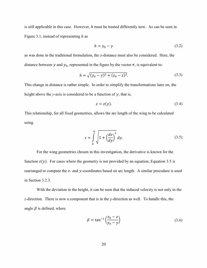
is still applicable in this case. However, must be treated differently now. As can be seen in

Figure 3.1, instead of representing as

(3.2)

as was done in the traditional formulation, the z-distance must also be considered. Here, the

distance between and , represented in the figure by the vector , is equivalent to:

√( ) (𝑧 𝑧) (3.3)

This change in distance is rather simple. In order to simplify the transformations later on, the

height above the y-axis is considered to be a function of ; that is,

𝑧 𝑧( ) (3.4)

This relationship, for all fixed geometries, allows the arc length of the wing to be calculated

using

∫√ ( 𝑧

)

(3.5)

For the wing geometries chosen in this investigation, the derivative is known for the

function 𝑧( ). For cases where the geometry is not provided by an equation, Equation 3.5 is

rearranged to compute the 𝑧- and -coordinates based on arc length. A similar procedure is used

in Section 3.2.3.

With the deviation in the height, it can be seen that the induced velocity is not only in the

z-direction. There is now a component that is in the y-direction as well. To handle this, the

angle is defined, where

(𝑧 𝑧

) (3.6)

21

The total induced velocity in the z-direction at by the vortex filament located at 𝑧 is

given as:

𝑉

√( ) (𝑧 𝑧) (3.7)

However, since the wing is not flat, and the bound vortex will generate a velocity normal to the

incoming velocity and direction of the vortex filament at 𝑧 , the normal direction of the wing

at 𝑧 must also be considered. For the normal direction at 𝑧 given by , the angle

between the z-axis and is an angle of interest. This angle is called . With this angle, the

induced velocity normal to the wing at 𝑧 is:

𝑉

√( ) (𝑧 𝑧) ( ) (3.8)

The closer the influencing trailing vortex is to the control point, the closer to unity

𝑜 ( ) will be, supposing the wing shape is continuous and the vortex filament and control

point are on the same half of the wing.

Since the wing is no longer planar, the self-influence of the bound vortex must be

considered. It is clear, that the more the wing shape deviates from being planar, the more

𝑧

𝑧

𝑧

Figure 3.1 Generic Non-Planar Wing with Induced Velocities

22

significant the self-induced velocity would be. However, in this analysis, this self-induction has

been treated as negligible. This has been done for two primary reasons.

The first reason is that for most practical configurations, the deflection of the wing is

relatively small. As such, the angle between two sections of the bound vortex would be

relatively small, reducing the induced velocity upon itself. The induced lift from these cases

would negligible. This idea was originally substantiated by Cone.14

The second reason is for ease of computation. When considering the influence of the

bound vortex on itself, there would be a discontinuity at the control point. The handling of this

discontinuity would be non-trivial and if handled incorrectly, could reduce rather than increase

the accuracy of the solution.

If the necessary changes to the governing equation due to the change in geometry are

examined, it can be seen that the formulation remains very similar to the classical formulation.

When the required changes are substituted back into Equation 2.10 for induced angle of attack,

the result is:

( )

𝑉 ∫

(

)

√( ) (𝑧 𝑧) ( )

(3.9)

Since the freestream velocity is unchanged, and the assumption that the incoming wind is at a

small angle to the wing is retained, the induced angle of attack remains familiar.

It is important to remember that this induced angle of attack at is a local induced

angle; the angle is relative to the normal of the wing at the control point, not the y-axis.

If this modified induced angle of attack is included in the governing equation, they

become:

23

( ) ( )

𝑉 ( ) ( )

𝑉 ∫

(

)

√( ) (𝑧 𝑧) ( )

(3.10)

While 𝑧 terms are included currently in the integrand, there is still only one unknown, ( ), as

the geometry of the wing is defined. Furthermore, and are known and are relative to

the normal direction at the control point.

3.2 Specific Formulations

While the general formulation of the problem is strikingly similar to the traditional

formulation, it can be seen that the integration is non-trivial and for every case examined in this

investigation, requires numerical methods to compute. As it would be impossible to adequately

cover every case of a deformed wing in any succinct manner, this investigation focuses on two

specific cases: simple dihedral and an aeroelastic model. Each of these requires its own

simplification and handling.

3.2.1 Dihedral

Let the wing be made of two identical semi-span pieces, joined at the origin. Further,

each half of the wing is inclined at an angle from the y-axis. As can be seen in Figure 3.2, if

the semi-span of each half-wing, , is kept the same, then there are three simplifications in the

governing equation: the projected span, the denominator for the induced angle of attack, and the

definition of 𝑜 ( ) in the integrand.

24

Starting with the cosine term in the integrand, it can be seen that is constant on either

side. Moreover, if the control point and the inducing vortex are on the same half of the wing, the

cosine term disappears completely, as .

Using Figure 3.2, the projected span can be represented simply by:

(3.11)

Similarly, the 𝑧 components can be expressed as a function of as well:

𝑧( ) (3.12)

As this dihedral is constant for a case and across the whole wing, this definition is substituted

into the denominator of Equation 3.8:

√( ) (𝑧 𝑧) √( ) ( ) (3.13)

Relating the arc-length and the y and z-coordinates is simple for this case, as it is merely

the hypotenuse of the triangle along one side of the wing. Therefore, the arc-length is:

√ 𝑧 (3.14)

Because the relationship between y and z is known, it is possible to calculate every value needed

for the governing equation, which becomes:

V

r

( )

𝑧

𝑧

𝑧

s

Figure 3.2 Dihedral Wing with Induced Velocities

V

r

( )

s

25

( ) ( )

𝑉 ( ) ( )

𝑉 ∫

(

)

√( ) ( ) ( )

(3.15)

It is important to remember that , , , and are all functions of . The variable is

used because it keeps the governing equation cleaner. The substitution of arc-length, , into the

denominator yields no simplification of the integration or increased insight into the character of

the equation.

3.2.2 Deformable Wing

Until this point, all cases of wing geometry have been presented as rigid. However, this

assumption can be removed to extend the investigation into static aeroelasticity.

Assume the starting wing can be any geometry fitting the criteria for Chapters 2 or 3. For

simplicity, the cases considered in this investigation will initially be flat. Using the governing

lifting line equation for the given planform, and can be determined for the wing.

Moreover, since is known, the lift distribution is known across the wing. The distributed

loading, ( ), is determined using the resultant lift coefficients and the freestream quantities

and 𝑉 . For the initial case of a flat wing, bending force applied to the wing is equal to the lift,

( ) 𝑉 ( ) (3.16)

The governing equation, Equation 3.10, results in the force normal to the wing, independent of

the shape of the wing. When the wing is not flat, the lift is calculated using the angle between

the z-direction and the local normal vector of the wing.

The wing is modeled using a simple finite element method. It is assumed that

deformations are limited to the y-z plane and that lift distribution does not affect twist. The wing

26

is divided into discrete “beams” along the lifting line to model bending. Each of these beams is

represented using a local stiffness matrix:

{

}

[

[

] [

]

[

] [

]] {

𝑧

𝑧

} (3.17)

Expressing this in more condensed form,

{ } [ ]{ } (3.18)

such that

[ ] [

] (3.19)

with each a 2x2 matrix.

The wing is represented by elements. Since the loads on the wing are symmetric, the

wing is considered starting from the midspan to one wingtip, the results mirrored to the other

half. To accurately model the wing, each of the local stiffness matrices is combined together to

create a global stiffness matrix of the form:

[ ]

[

]

with { }

{

𝑧

𝑧

𝑧

}

. (3.20)

The wing is modeled as a cantilevered beam. Therefore, the deflection and slope at the

root are uniformly zero, or:

𝑧 (3.21)

27

It can be seen that when performing the matrix multiplication, the boundary conditions imposed

remove the first two rows and columns of the global stiffness matrix (elements ,

, and

) leaving:

[ ] [

] (3.22)

The resultant governing equation for the bending then becomes:

{

}

[ ]

{

𝑧

𝑧

}

(3.23)

It is possible to separate the global stiffness matrix into 4 matrices such that:

{{ } [ ]{𝑧} [ ]{ }

{ } [ ]{𝑧} [ ]{ } (3.24)

Since there are no moments applied to the wing, that is:

(3.25)

the resulting set of equations takes the following form:

{{ } [ ]{𝑧} [ ]{ }

{ } [ ]{𝑧} [ ]{ } (3.26)

By solving the second equation for and substituting it into the first, the equation to solve for the

deflections becomes:

{ } [[ ] [ ][ ] [ ]]{𝑧} (3.27)

The solution of this system of linear equations provides the deflection of the end point of each

panel.

28

Now that the deflections are known, the lifting line model can be used upon the newly

deformed wing. The only change in the governing lifting line equation is that the z-locations and

consequently the normal vectors of the control points are defined through the bending model.

If it is assumed that the panels themselves are rigid, that is the deflection occurs only at

the end points and the panels are at a constant slope between end points, then the model is

greatly simplified. For each panel the normal is then defined as:

𝑧 𝑧

(3.28)

The governing aerodynamic equation, Equation 3.10, is solved using a collocation

method, which provides the forces generated at the mid-point of the elements. The governing

bending equation, Equation 3.17, requires the forces at the end-points of each panel. In order to

match the two distributions, the normal force on the ith-panel was split equally between its end-

points. That is, for end-points and , we have:

( ) ( )

(3.29)

3.3 Solution to Non-Planar Formulations

The solution of the non-planar formulation of the lifting-line equation is quite similar to

that of the traditional formulation, in that a general lift distribution is solved for using the

collocation method. As was stated earlier, the influence of the bound vortex on itself is not

considered in this solution.

For the collocation method used in this investigation, the wing was divided into N

discrete panels, each with a control point at its center. These panels created a set of linear

equations that were solved simultaneously, providing the Fourier coefficients. The coefficients

were then used to compute the lift and drag coefficients across the wing.

29

The calculation of the drag was performed in the same manner as for the traditional

formulation. As before, the Cartesian coordinates are converted to polar coordinates using the

transformation:

(3.30)

However, since the wings were non-planar in this investigation, it was necessary to consider the

normal of the wing when calculating the lift. The normal force coefficient was simple to

calculate, as it is the force perpendicular to the wing at all points, and therefore given directly by

the Fourier series:

∑

∫

(3.31)

In order to calculate the lift, the angle between the z-axis and the local normal of the wing was

taken into consideration. This modified the integral to be:

∑

∫

(3.32)

The additional term is also a function of . In order to solve this integral for the current

formulation, the integration was carried out numerically.

Recalling Equation 3.8, it can be seen that while integrating across the control point, the

induced angle of attack becomes undefined. To resolve this singularity, the wing was treated in

two pieces, with the section of the wing immediately around the discontinuity considered

separately from the majority of the wing. Outside the region immediately surrounding the

singularity, the integration was performed using Simpson’s rule; across the singularity, the

30

integration was performed using the trapezoid rule. This prevented evaluation of the function at

the singular point.

It should also be noted here that the governing equation contains the aspect ratio, which

has an effect of the characteristics of the wing, as was shown in Chapter 2. A decision was

required in this investigation whether the actual or the projected span of the wing would be used.

For many cases, the effect of the change in the aspect ratio could be considered negligible.

However, for the larger deflections, which would be expected to have a larger variation from

planar aerodynamic characteristics, the aspect ratio could vary significantly. It was decided,

therefore, to use the projected span of the wing. This decision was believed to account for the

amount of the normal force in the lifting direction, given by the first term on the right hand side

of Equation 3.9, generated by the un-influenced wing.

31

CHAPTER 4

RESULTS AND DISCUSSION

In this chapter, the results from the classical solution and the current formulation are

presented and discussed. The classical results are used for validation. The sensitivity of the

problem to the number of spanwise panels was determined with the comparison of the Fourier

coefficients obtained through the classical solution. These Fourier coefficients were then used to

determine the number of subdivisions required for the numerical integration used in the present

formulation.

In the present solution, the case of a wing with dihedral and an initially flat, deformable

wing were considered in detail. For dihedral, this investigation focused on the lift-curve slope

and induced drag of the planforms considered to determine the effect of non-planar geometries.

For deformable cases, in addition to induced drag and lift-curve slope, the effect different

planforms had on wing shape after bending was also considered.

4.1 Convergence Analysis

4.1.1 Number of Panels

In order to determine the number of panels needed for the simulation, 3 cases were

examined. The cases were run at an angle of attack of 4 degrees with a wing of AR = 10. The

first case considered was a rectangular wing with no twist; the second case an untwisted but

tapered wing with ; the final case as that of a rectangular wing with a linear two-

degree washout. All solutions were obtained with 8, 16, 32, and 64 panels.

As can be seen in work performed by Rasmussen and Smith,6 an increase in the number

of panels results in the convergence of the individual coefficients towards an asymptotic value.

To compare the effect of additional panels on the individual coefficients, the Fourier coefficients

32

were first normalized relative to the values obtained using 64 panels. The normalized

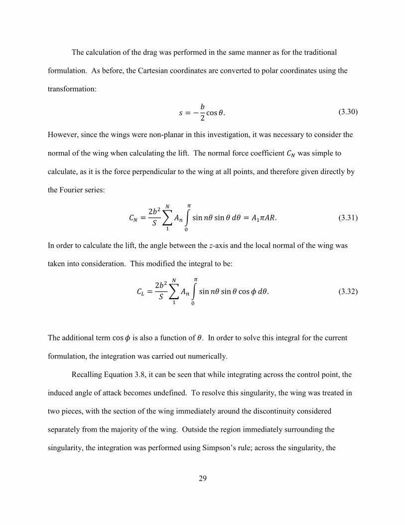
coefficients were then compared as the number of panels was changed. The results are shown in

Figure 4.1.

As can be seen in Figure 4.1, the first 3 non-zero Fourier coefficients converged quickly

for the untwisted rectangular wing. For all solutions obtained using more than 8 panels, each of

the coefficients was within 0.5% of the value at 64 panels. The circulation distribution, seen in

Figure 4.2, confirmed the quick convergence of the solution. Part (a) of Figure 4.2 shows an

overview of the distribution over the semi-span, with Part (b) showing a detailed view of the

differences in the circulation distributions inboard of . The distributions for 16, 32

and 64 panels cannot be distinguished from each other. Thus from the rectangular wing, it was

determined that a minimum of 16 panels would need to be used for reasonable convergence.

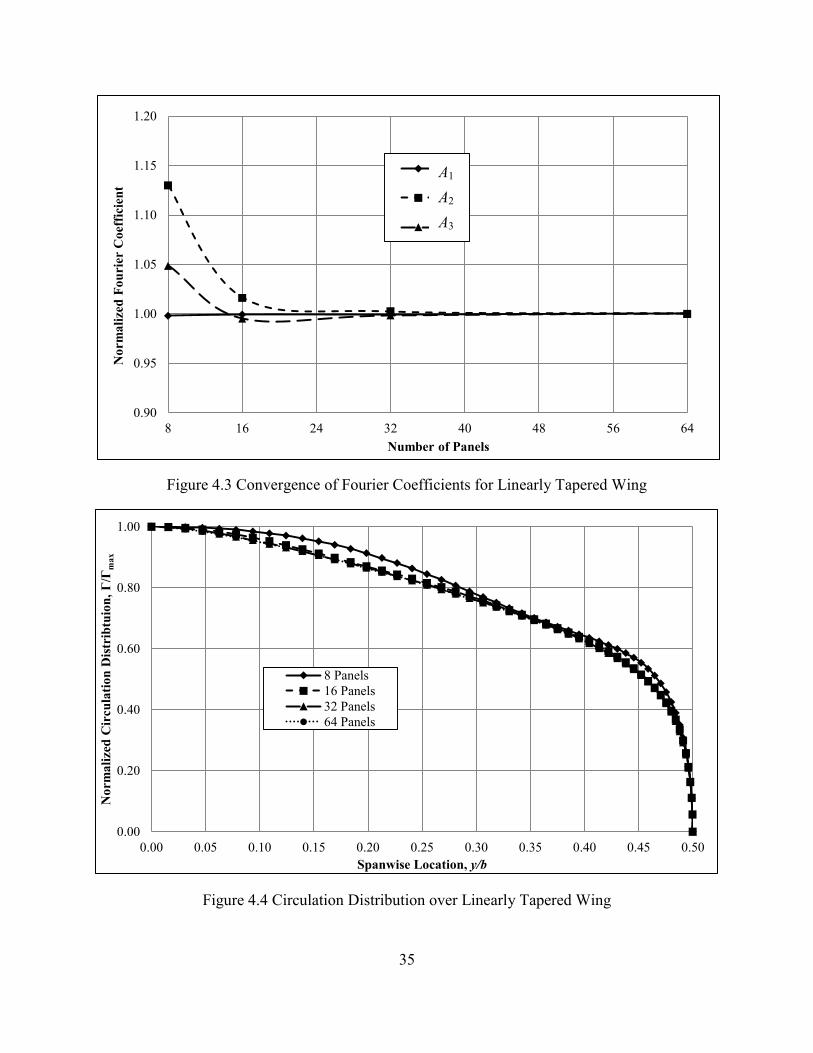
When the more complex, tapered wing case was considered, 16 panels did not lead to a

converged solution. As can be seen in Figure 4.3, the Fourier coefficients for 16 panels still

displayed as much as 1.6% difference from the 64-panel case. This was reinforced by the

circulation distribution seen in Figure 4.4. The 8- and 16-panel cases showed deviation from the

other two curves. The 32- panel case agreed well with the 64-panel case. The maximum

deviation in the first 3 coefficients was less than 0.2% between the 32-panel and the 64-panel

cases. While larger percent differences were seen in higher order coefficients, the magnitudes of

the coefficients where these errors manifested were significantly less than the first coefficients.

It was determined that based on this geometry, a minimum of 32 panels would be needed.

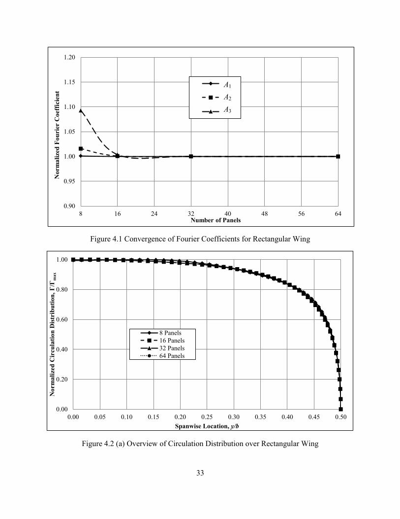
33

Figure 4.1 Convergence of Fourier Coefficients for Rectangular Wing

Figure 4.2 (a) Overview of Circulation Distribution over Rectangular Wing

0.90

0.95

1.00

1.05

1.10

1.15

1.20

8 16 24 32 40 48 56 64

Nor

mal

ized

Fou

rier

Coe

ffic

ient

Number of Panels

A1

A3

A5

0.00

0.20

0.40

0.60

0.80

1.00

0.00 0.05 0.10 0.15 0.20 0.25 0.30 0.35 0.40 0.45 0.50

Nor

mal

ized

Cir

cula

tion

Dis

trib

utio

n, Γ

/Γm

ax

Spanwise Location, y/b

8 Panels16 Panels32 Panels64 Panels

A1

A2

A3

34

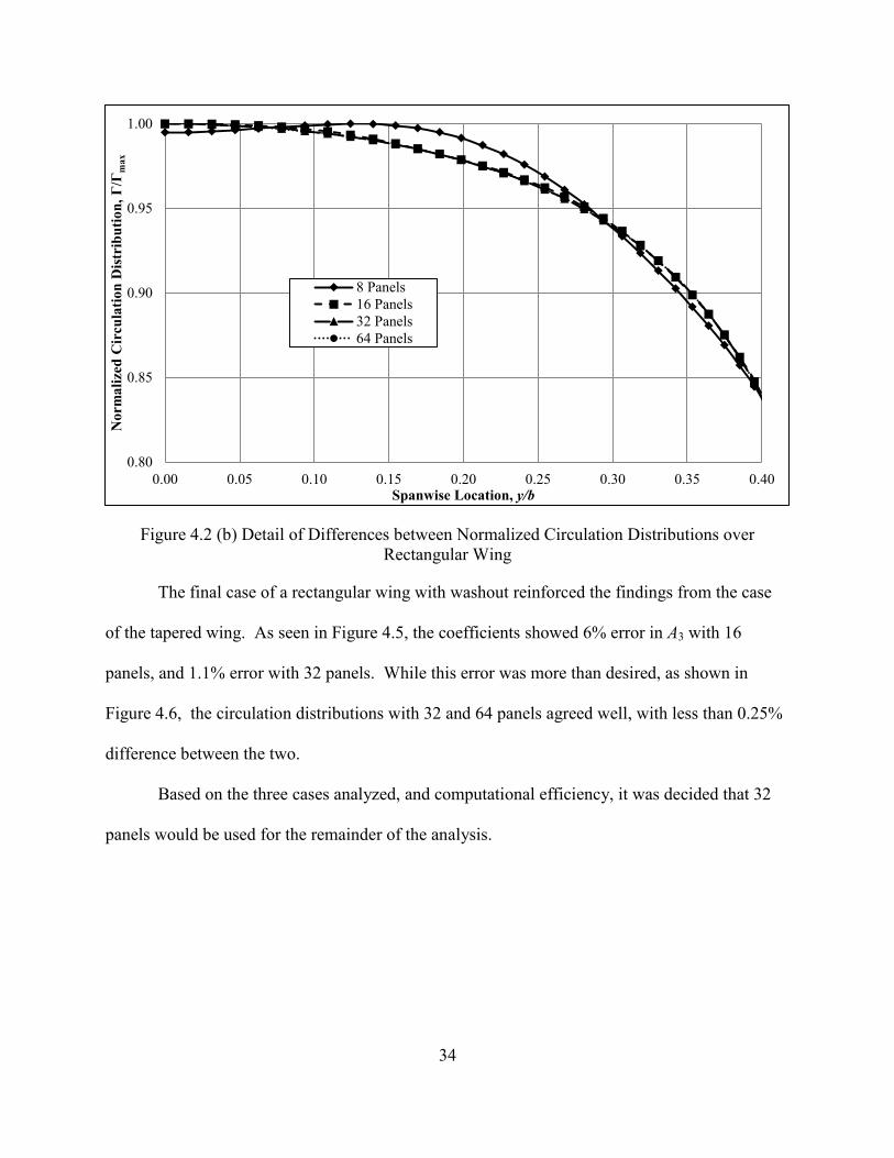
Figure 4.2 (b) Detail of Differences between Normalized Circulation Distributions over Rectangular Wing

The final case of a rectangular wing with washout reinforced the findings from the case

of the tapered wing. As seen in Figure 4.5, the coefficients showed 6% error in A3 with 16

panels, and 1.1% error with 32 panels. While this error was more than desired, as shown in

Figure 4.6, the circulation distributions with 32 and 64 panels agreed well, with less than 0.25%

difference between the two.

Based on the three cases analyzed, and computational efficiency, it was decided that 32

panels would be used for the remainder of the analysis.

0.80

0.85

0.90

0.95

1.00

0.00 0.05 0.10 0.15 0.20 0.25 0.30 0.35 0.40

Nor

mal

ized

Cir

cula

tion

Dis

trib

utio

n, Γ

/Γm

ax



35

Figure 4.3 Convergence of Fourier Coefficients for Linearly Tapered Wing

Figure 4.4 Circulation Distribution over Linearly Tapered Wing

0.90

0.95

1.00

1.05

1.10

1.15

1.20

8 16 24 32 40 48 56 64

Nor

mal

ized

Fou

rier

Coe

ffic

ient

Number of Panels

A1

A3

A5

0.00

0.20

0.40

0.60

0.80

1.00

0.00 0.05 0.10 0.15 0.20 0.25 0.30 0.35 0.40 0.45 0.50

Nor

mal

ized

Cir

cula

tion

Dis

trib

tuio

n, Γ

/Γm

ax



A1

A2

A3

36

Figure 4.5 Convergence of Fourier Coefficients for Rectangular Wing with Linear Washout

Figure 4.6 Circulation Distribution over Rectangular Wing with Linear Washout

0.90

0.95

1.00

1.05

1.10

1.15

1.20

8 16 24 32 40 48 56 64

Nor

mal

ized

Fou

rier

Coe

ffic

ient

Number of Panels

A1

A3

A5

0.00

0.20

0.40

0.60

0.80

1.00

0.00 0.05 0.10 0.15 0.20 0.25 0.30 0.35 0.40 0.45 0.50

Nor

mal

ized

Cir

cula

tion

Dis

trib

utio

n, Γ

/Γm

ax



A1

A2

A3

37

4.1.2 Numerical Integration Subdivisions

The integration was performed using Simpson’s rule over the majority of the wing, with a

simplification to the Trapezoidal rule across the discontinuity to avoid evaluating the integrand at

the discontinuity, as discussed in Chapter 3. Initial runs were made with 200, 300, 400, and 500

subdivisions within each panel over the linearly washed-out and tapered wing. It was noted that

these cases required an excessive amount of time, without any difference in the Fourier

coefficients. As such, it was determined that significantly fewer subdivisions were needed than

first believed.

Simulations were then run with 20, 50, and 100 subdivisions per panel. As expected, the

runs took significantly less time. Minimal increase in the time for the simulation was noted

between the 20- and 50-subdivision cases. The difference between the analytical and numerical

solutions in the Fourier coefficients was seen to be less than 0.1% for all coefficients. For most

Fourier coefficients, the difference was significantly less. A minimal increase in accuracy

between the 20- and 50-subdivision cases was noted, but a negligible increase in accuracy was

obtained when 100 subdivisions were used.

Due to the minimal increase in computational time, it was determined that using 50

subdivisions per panel was beneficial as the behavior of the circulation distribution was unknown

for non-planar geometries.

4.2 Wing with Dihedral

4.2.1 Effect of Aspect Ratio

The results of running 3 cases of a flat wing and the same wings with 6 degrees of

dihedral at aspect ratios of 6, 10, and 14 showed the classical trends of aspect ratio to be

insensitive to dihedral. The three cases run were of a rectangular wing, a wing with 50% linear

38

taper, and a wing with 50% linear taper and 2 degrees of linear washout. Figure 4.7 parts (a) and

(b) present the lift-curve for the rectangular wing for the flat and dihedral cases, respectively.

The trends showed that an increase of aspect ratio corresponded to an increase of lift-curve slope.

Additionally, the percentage increase of the lift-curve slope due to increase of aspect ratio

remained constant between flat and dihedral cases.

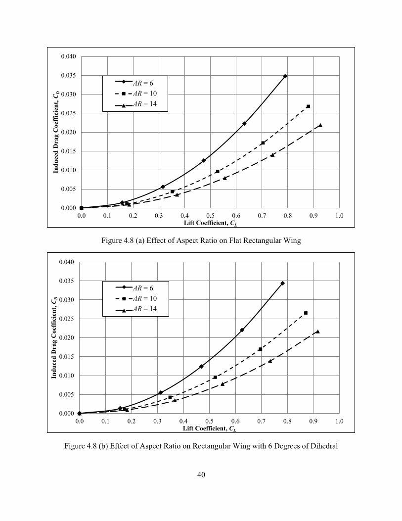
Figure 4.8 displays the representative drag polars for the rectangular wing. An increase

in aspect ratio resulted in a decrease in induced drag. Similar plots for the wings with taper and

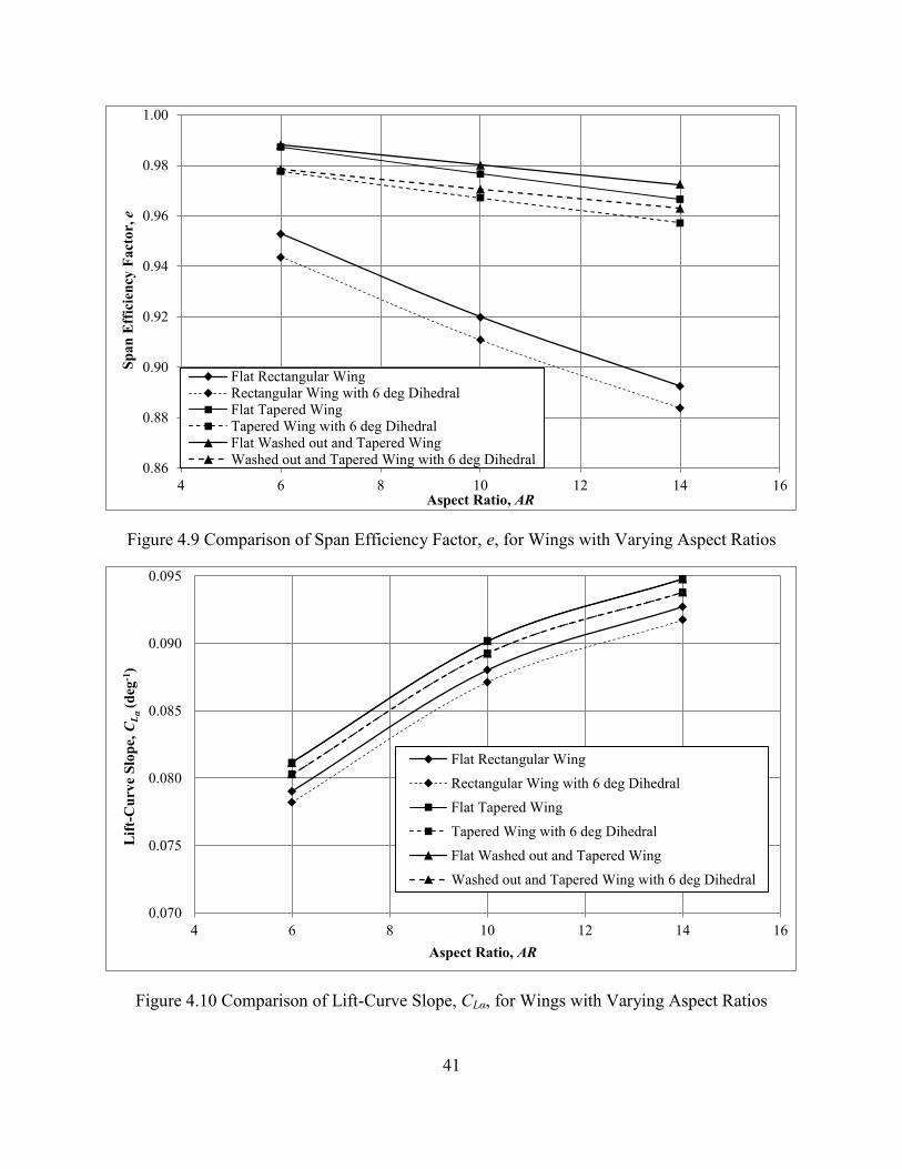
washout were not included as the form was the same as for the rectangular wing. In Figure 4.9

the span efficiency factor, e, is plotted for all three wings at both . The offset

between the solid ( ) and dashed ( ) series shows the constant decrease in e,

regardless of aspect ratio and wing geometry. A similar constant offset is seen in the lift-curve

slope in Figure 4.10. It should be noted that the lift-curve slope is independent of washout,

causing the plots of the tapered wing without and with washout to lie on top of each other.

Geometric and aerodynamic twist alter , which is combined with when solving

Equation 3.10. Washout does not affect directly the integral in the governing equation.

As the trends of aspect ratio were found to be independent of dihedral, the dihedral cases

were run at a single aspect ratio .

39

Figure 4.7 (a) Effect of Aspect Ratio on Lift-Curve Slope of Flat Rectangular Wing

Figure 4.7 (b) Effect of Aspect Ratio on Lift-Curve Slope of Rectangular Wing with 6 Degrees of Dihedral

0.0

0.1

0.2

0.3

0.4

0.5

0.6

0.7

0.8

0.9

1.0

0 1 2 3 4 5 6 7 8 9 10

Lift

Coe

ffic

ient

, CL

Angle of Attack, α (deg)

AR = 6AR = 10AR = 14

0.0

0.1

0.2

0.3

0.4

0.5

0.6

0.7

0.8

0.9

1.0

0 1 2 3 4 5 6 7 8 9 10

Lift

Coe

ffic

ient

, CL


AR = 6

AR = 10

AR = 14

AR = 6 AR = 10 AR = 14

AR = 6 AR = 10 AR = 14

40

Figure 4.8 (a) Effect of Aspect Ratio on Flat Rectangular Wing

Figure 4.8 (b) Effect of Aspect Ratio on Rectangular Wing with 6 Degrees of Dihedral

0.000

0.005

0.010

0.015

0.020

0.025

0.030

0.035

0.040

0.0 0.1 0.2 0.3 0.4 0.5 0.6 0.7 0.8 0.9 1.0

Indu

ced

Dra

g C

oeff

icie

nt, C

D

Lift Coefficient, CL

AR = 6

AR = 10

AR = 14

0.000

0.005

0.010

0.015

0.020

0.025

0.030

0.035

0.040

0.0 0.1 0.2 0.3 0.4 0.5 0.6 0.7 0.8 0.9 1.0

Indu

ced

Dra

g C

oeff

icie

nt, C

D


AR = 6

AR = 10

AR = 14

AR = 6 AR = 10 AR = 14

AR = 6 AR = 10 AR = 14

41

Figure 4.9 Comparison of Span Efficiency Factor, e, for Wings with Varying Aspect Ratios

Figure 4.10 Comparison of Lift-Curve Slope, CLα, for Wings with Varying Aspect Ratios

0.86

0.88

0.90

0.92

0.94

0.96

0.98

1.00

4 6 8 10 12 14 16

Span

Eff

icie

ncy

Fact

or, e

Aspect Ratio, AR

Flat Rectangular WingRectangular Wing with 6 deg DihedralFlat Tapered WingTapered Wing with 6 deg DihedralFlat Washed out and Tapered WingWashed out and Tapered Wing with 6 deg Dihedral

0.070

0.075

0.080

0.085

0.090

0.095

4 6 8 10 12 14 16

Lift

-Cur

ve S

lope

, CL α

(deg

-1)

Aspect Ratio, AR

Flat Rectangular WingRectangular Wing with 6 deg DihedralFlat Tapered WingTapered Wing with 6 deg DihedralFlat Washed out and Tapered WingWashed out and Tapered Wing with 6 deg Dihedral

42

4.2.2 Effect of Dihedral on an Elliptically Loaded Wing

It was found by Prandtl1 that an elliptically-loaded wing has the minimum induced drag

of any flat planform. Therefore, it was believed important to investigate the impact of dihedral

on an elliptically-loaded wing. The loading was produced using a wing of elliptical planform.

The first, and most notable characteristic of the results from the numerical solution was

that the wing with dihedral retained only one term in the Fourier series. This is similar to a flat

wing. Recalling Equation 3.1, the induced drag of the wing is:

∑

(3.1)

The reader is reminded that the minimum induced drag occurs when the only non-zero

coefficient in the series is A1. The result therefore showed that an elliptically loaded wing with

dihedral remains the most efficient planform.

While the minimum drag for a wing with dihedral exists with an elliptical load, adding

dihedral was found to decrease the lift-curve slope and increase the induced drag compared to

the flat wing. This decrease of lift-curve slope and span efficiency factor is due to the angular

offset between the local wing normal direction, , and lift direction (z-axis), as seen in Figure

3.2. In order to produce an equivalent lift to the flat wing, a wing with dihedral must generate

more load normal to the wing surface, so that the component of the normal force in the lift

direction is equivalent to that produced by the flat wing. The remaining portion of the normal

force given by:

(4.1)

produces additional drag without providing additional lift. The deviation of lift-curve slope from

that of the flat wing is shown in Table 4.1 and Figure 4.11.

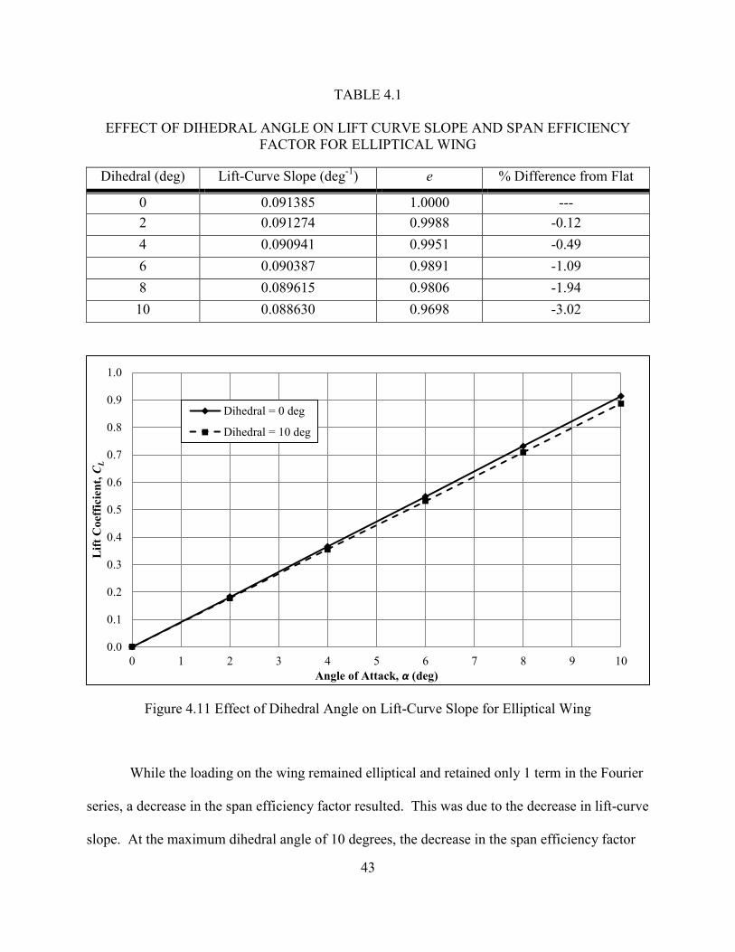
43

TABLE 4.1

EFFECT OF DIHEDRAL ANGLE ON LIFT CURVE SLOPE AND SPAN EFFICIENCY FACTOR FOR ELLIPTICAL WING

Dihedral (deg) Lift-Curve Slope (deg-1) e % Difference from Flat

0 0.091385 1.0000 --- 2 0.091274 0.9988 -0.12 4 0.090941 0.9951 -0.49 6 0.090387 0.9891 -1.09 8 0.089615 0.9806 -1.94 10 0.088630 0.9698 -3.02

Figure 4.11 Effect of Dihedral Angle on Lift-Curve Slope for Elliptical Wing

While the loading on the wing remained elliptical and retained only 1 term in the Fourier

series, a decrease in the span efficiency factor resulted. This was due to the decrease in lift-curve

slope. At the maximum dihedral angle of 10 degrees, the decrease in the span efficiency factor

0.0

0.1

0.2

0.3

0.4

0.5

0.6

0.7

0.8

0.9

1.0

0 1 2 3 4 5 6 7 8 9 10

Lift

Coe

ffic

ient

, CL


Dihedral = 0 deg

Dihedral = 10 deg

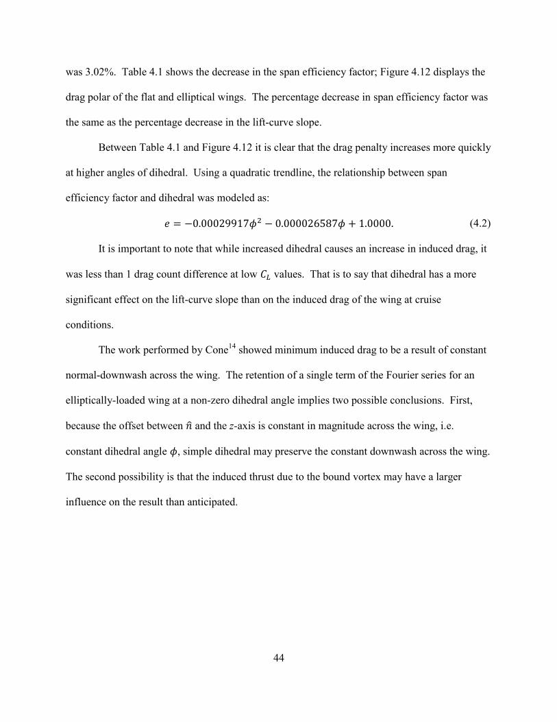
44

was 3.02%. Table 4.1 shows the decrease in the span efficiency factor; Figure 4.12 displays the

drag polar of the flat and elliptical wings. The percentage decrease in span efficiency factor was

the same as the percentage decrease in the lift-curve slope.

Between Table 4.1 and Figure 4.12 it is clear that the drag penalty increases more quickly

at higher angles of dihedral. Using a quadratic trendline, the relationship between span

efficiency factor and dihedral was modeled as:

𝑒 (4.2)

It is important to note that while increased dihedral causes an increase in induced drag, it

was less than 1 drag count difference at low values. That is to say that dihedral has a more

significant effect on the lift-curve slope than on the induced drag of the wing at cruise

conditions.

The work performed by Cone14 showed minimum induced drag to be a result of constant

normal-downwash across the wing. The retention of a single term of the Fourier series for an

elliptically-loaded wing at a non-zero dihedral angle implies two possible conclusions. First,

because the offset between and the z-axis is constant in magnitude across the wing, i.e.

constant dihedral angle , simple dihedral may preserve the constant downwash across the wing.

The second possibility is that the induced thrust due to the bound vortex may have a larger

influence on the result than anticipated.

45

Figure 4.12 Effect of Dihedral on Drag Coefficient of Elliptical Wing

Since the elliptically-loaded wing provided the minimum drag for both flat and dihedral

cases, it was used as a benchmark with which to compare the remaining dihedral cases.

Differences from these results for the elliptically-loaded wing showed a deviation from the

optimum at each dihedral angle.

4.2.3 Effect of Dihedral on Twist

To consider the effect of dihedral on a twisted rectangular wing, cases were run for 1, 2,

and 3 degrees of linear washout over the span. As was mentioned in Section 4.2.1, twist did not

affect the lift-curve slope. The decrease in lift-curve slope for a wing with washout was the same

as for an equivalent planform with no washout. As a result this section focuses solely on the

effect of dihedral on the induced drag of twisted wings.

0.000

0.005

0.010

0.015

0.020

0.025

0.030

0.00 0.10 0.20 0.30 0.40 0.50 0.60 0.70 0.80 0.90 1.00

Dra

g C

oeff

icie

nt, C

D


Dihedral = 0 deg

Dihedral = 10 deg

46

The washout on the wing produces a change in circulation over the wing as angle of

attack changes. This means that the span efficiency factor of each wing changes with angle of

attack. Figure 4.13 shows the effect that the angle of attack has on the span efficiency factor of a

wing with 1 degree of washout. At angles lower than the washout, the span efficiency factor of

the wing is significantly decreased due to the generation of negative lift on the outboard section

of the wing. It is also clear that this relationship between angle of attack and span efficiency

factor is independent of the dihedral angle of the wing.

To isolate the effect of dihedral on the trends in span efficiency factor due to washout,

data was obtained at three lift coefficients, . The results are shown in

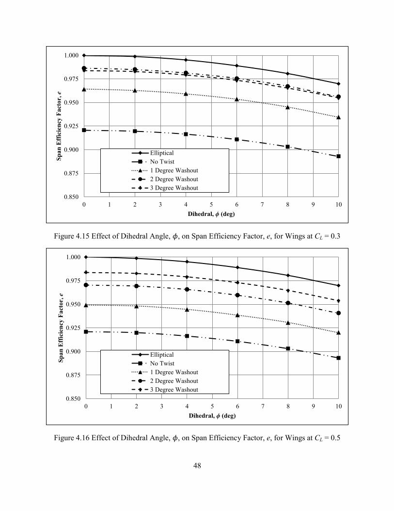
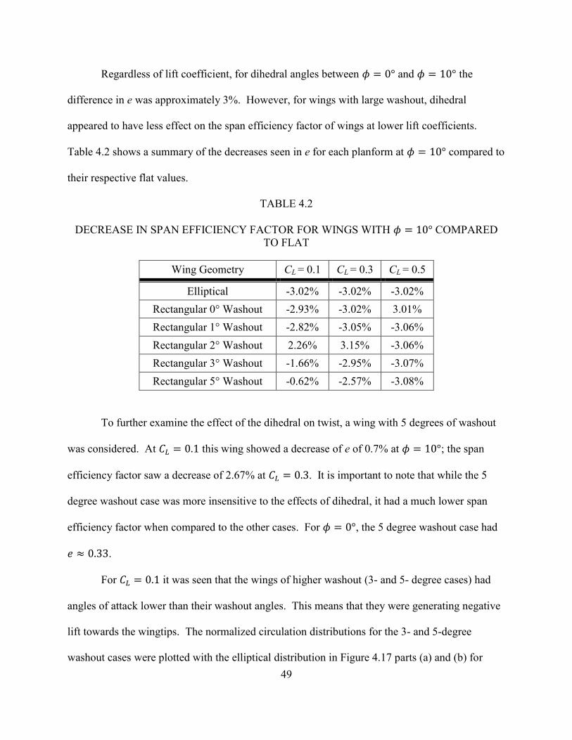
Figures 4.14, 4.15, and 4.16. As can be seen in Figure 4.14, at the lowest lift coefficient, the

wing with 1 degree washout was the most efficient of the twisted wings, with span efficiency

factor just lower than the elliptical wing at all dihedral angles. As the lift coefficient increased,

span efficiency factor was higher for wings with more washout. This can be seen in Figures 4.15

and 4.16.

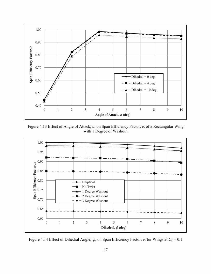
47

Figure 4.13 Effect of Angle of Attack, α, on Span Efficiency Factor, e, of a Rectangular Wing with 1 Degree of Washout

Figure 4.14 Effect of Dihedral Angle, , on Span Efficiency Factor, e, for Wings at CL = 0.1

0.40

0.50

0.60

0.70

0.80

0.90

1.00

0 1 2 3 4 5 6 7 8 9 10

Span

Eff

icie

ncy

Fact

or, e


Dihedral = 0 deg

Dihedral = 4 deg

Dihedral = 10 deg

0.60

0.65

0.70

0.75

0.80

0.85

0.90

0.95

1.00

0 1 2 3 4 5 6 7 8 9 10

Span

Eff

icie

ncy

Fact

or, e

Dihedral, ϕ (deg)

EllipticalNo Twist1 Degree Washout2 Degree Washout3 Degree Washout

48



0.850

0.875

0.900

0.925

0.950

0.975

1.000

0 1 2 3 4 5 6 7 8 9 10

Span

Eff

icie

ncy

Fact

or, e

Dihedral, ϕ (deg)


0.850

0.875

0.900

0.925

0.950

0.975

1.000

0 1 2 3 4 5 6 7 8 9 10

Span

Eff

icie

ncy

Fact

or, e

Dihedral, ϕ (deg)


49

Regardless of lift coefficient, for dihedral angles between and the

difference in e was approximately 3%. However, for wings with large washout, dihedral

appeared to have less effect on the span efficiency factor of wings at lower lift coefficients.

Table 4.2 shows a summary of the decreases seen in e for each planform at compared to

their respective flat values.

TABLE 4.2

DECREASE IN SPAN EFFICIENCY FACTOR FOR WINGS WITH COMPARED TO FLAT

Wing Geometry CL = 0.1 CL = 0.3 CL = 0.5

Elliptical -3.02% -3.02% -3.02% Rectangular 0° Washout -2.93% -3.02% 3.01% Rectangular 1° Washout -2.82% -3.05% -3.06% Rectangular 2° Washout 2.26% 3.15% -3.06% Rectangular 3° Washout -1.66% -2.95% -3.07% Rectangular 5° Washout -0.62% -2.57% -3.08%

To further examine the effect of the dihedral on twist, a wing with 5 degrees of washout

was considered. At this wing showed a decrease of e of 0.7% at ; the span

efficiency factor saw a decrease of 2.67% at . It is important to note that while the 5

degree washout case was more insensitive to the effects of dihedral, it had a much lower span

efficiency factor when compared to the other cases. For , the 5 degree washout case had

𝑒 .

For it was seen that the wings of higher washout (3- and 5- degree cases) had

angles of attack lower than their washout angles. This means that they were generating negative

lift towards the wingtips. The normalized circulation distributions for the 3- and 5-degree

washout cases were plotted with the elliptical distribution in Figure 4.17 parts (a) and (b) for

50

and respectively. What can be seen is the slight decrease of negative

circulation at the wingtips when = 10°. Producing less negative circulation, and therefore lift,

decreases the amount of drag being produced without corresponding lift. It should be noted that

there is an increase in maximum circulation between flat and dihedral cases of between 0.5% and

1% for the washout cases.

In order eliminate the negative lift at the wingtips, the angle of attack was increased. The

spanwise circulation distribution was examined at . The results are plotted in Figure

4.18 parts (a) and (b) for and respectively. As is apparent from the plot, the

difference between flat and dihedral cases was primarily the magnitude of the circulation

generated; higher angles of dihedral required slightly more circulation to create the same lift.

Normalizing the circulation over the wing allowed comparisons of the character of the

spanwise distribution. The normalized spanwise circulation can be seen in Figure 4.19 (a) and

(b). There is no significant difference in the shape of the distributions. When the lines are

placed on the same plot, the only visible difference was in the case of 3 degrees of washout,

which had a slight offset in the slope of the distribution outboard of

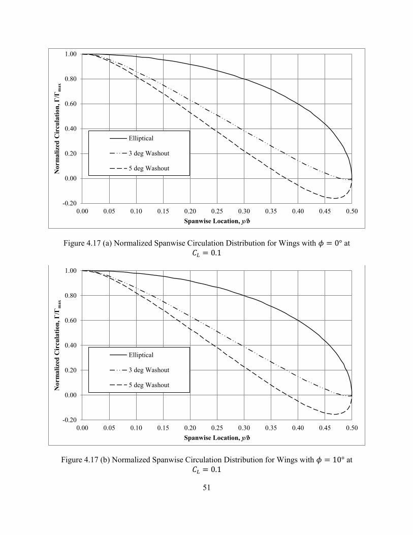
51

Figure 4.17 (a) Normalized Spanwise Circulation Distribution for Wings with at

Figure 4.17 (b) Normalized Spanwise Circulation Distribution for Wings with at

-0.20

0.00

0.20

0.40

0.60

0.80

1.00

0.00 0.05 0.10 0.15 0.20 0.25 0.30 0.35 0.40 0.45 0.50

Nor

mal

ized

Cir

cula

tion,

Γ/Γ

max


Elliptical

3 deg Washout

5 deg Washout

-0.20

0.00

0.20

0.40

0.60

0.80

1.00

0.00 0.05 0.10 0.15 0.20 0.25 0.30 0.35 0.40 0.45 0.50

Nor

mal

ized

Cir

cula

tion,

Γ/Γ

max


Elliptical

3 deg Washout

5 deg Washout

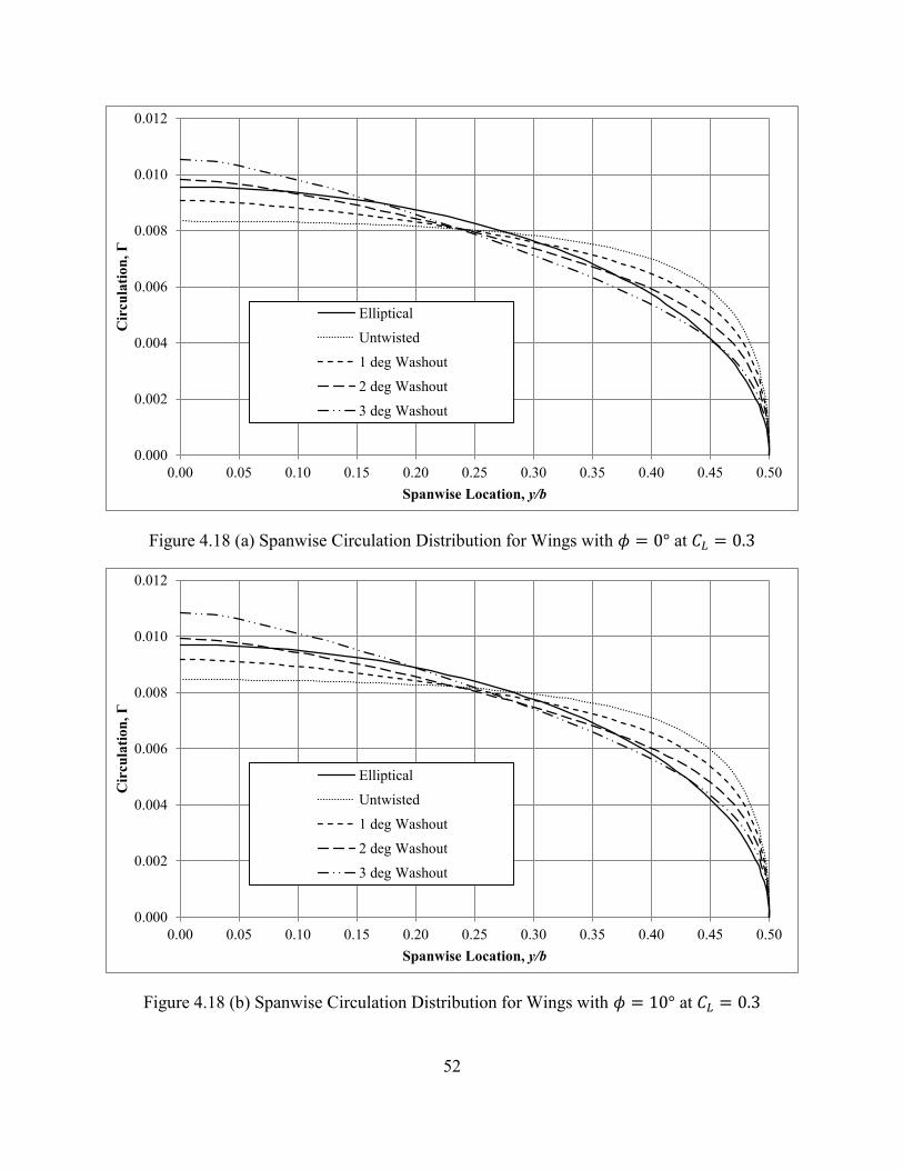
52

Figure 4.18 (a) Spanwise Circulation Distribution for Wings with at

Figure 4.18 (b) Spanwise Circulation Distribution for Wings with at

0.000

0.002

0.004

0.006

0.008

0.010

0.012

0.00 0.05 0.10 0.15 0.20 0.25 0.30 0.35 0.40 0.45 0.50

Cir

cula

tion,

Γ


Elliptical

Untwisted

1 deg Washout

2 deg Washout

3 deg Washout

0.000

0.002

0.004

0.006

0.008

0.010

0.012

0.00 0.05 0.10 0.15 0.20 0.25 0.30 0.35 0.40 0.45 0.50

Cir

cula

tion,

Γ


Elliptical

Untwisted

1 deg Washout

2 deg Washout

3 deg Washout

53

Figure 4.19 (a) Normalized Spanwise Circulation Distribution for Wings with at

Figure 4.19 (b) Normalized Spanwise Circulation Distribution for Wings with at

0.00

0.10

0.20

0.30

0.40

0.50

0.60

0.70

0.80

0.90

1.00

0.00 0.05 0.10 0.15 0.20 0.25 0.30 0.35 0.40 0.45 0.50

Nor

mal

ized

Cir

cula

tion,

Γ/Γ

max


EllipticalUntwisted1 deg Washout2 deg Washout3 deg Washout

0.00

0.10

0.20

0.30

0.40

0.50

0.60

0.70

0.80

0.90

1.00

0.00 0.05 0.10 0.15 0.20 0.25 0.30 0.35 0.40 0.45 0.50

Nor

mal

ized

Cir

cula

tion,

Γ/Γ

max


EllipticalUntwisted1 deg Washout2 deg Washout3 deg Washout

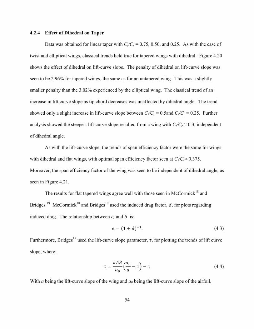
54

4.2.4 Effect of Dihedral on Taper

Data was obtained for linear taper with Ct/Cr = 0.75, 0.50, and 0.25. As with the case of

twist and elliptical wings, classical trends held true for tapered wings with dihedral. Figure 4.20

shows the effect of dihedral on lift-curve slope. The penalty of dihedral on lift-curve slope was

seen to be 2.96% for tapered wings, the same as for an untapered wing. This was a slightly

smaller penalty than the 3.02% experienced by the elliptical wing. The classical trend of an

increase in lift curve slope as tip chord decreases was unaffected by dihedral angle. The trend

showed only a slight increase in lift-curve slope between Ct/Cr = 0.5and Ct/Cr = 0.25. Further

analysis showed the steepest lift-curve slope resulted from a wing with Ct/Cr ≈ 0.3, independent

of dihedral angle.

As with the lift-curve slope, the trends of span efficiency factor were the same for wings

with dihedral and flat wings, with optimal span efficiency factor seen at Ct/Cr≈ 0.375.

Moreover, the span efficiency factor of the wing was seen to be independent of dihedral angle, as

seen in Figure 4.21.

The results for flat tapered wings agree well with those seen in McCormick18 and

Bridges.19 McCormick18 and Bridges19 used the induced drag factor, , for plots regarding

induced drag. The relationship between e, and is:

𝑒 ( ) (4.3)

Furthermore, Bridges19 used the lift-curve slope parameter, , for plotting the trends of lift curve

slope, where:

(

) (4.4)

With a being the lift-curve slope of the wing and a0 being the lift-curve slope of the airfoil.

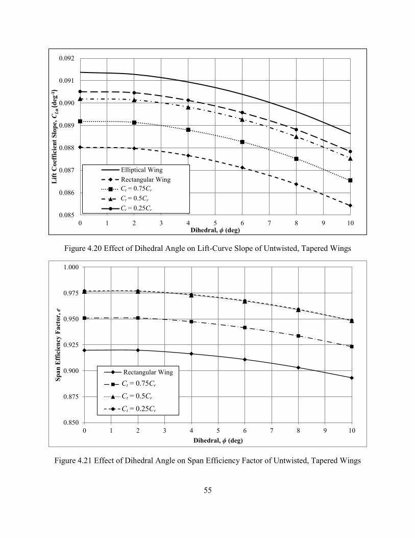
55

Figure 4.20 Effect of Dihedral Angle on Lift-Curve Slope of Untwisted, Tapered Wings

Figure 4.21 Effect of Dihedral Angle on Span Efficiency Factor of Untwisted, Tapered Wings

0.085

0.086

0.087

0.088

0.089

0.090

0.091

0.092

0 1 2 3 4 5 6 7 8 9 10

Lift

Coe

ffic

ient

Slo

pe, C

Lα (d

eg-1

)

Dihedral, ϕ (deg)

Elliptical WingRectangular WingCt = 0.75 CrCt = 0.5 CrCt = 0.25 Cr

0.850

0.875

0.900

0.925

0.950

0.975

1.000

0 1 2 3 4 5 6 7 8 9 10

Span

Eff

icie

ncy

Fact

or, e

Dihedral, ϕ (deg)

Rectangular Wing

Ct=0.75Cr

Ct=0.50Cr

Ct=0.25Cr

Ct = 0.75Cr Ct = 0.5Cr Ct = 0.25Cr

Ct = 0.75Cr

Ct = 0.5Cr

Ct = 0.25Cr

56

4.3 Deformable Wing

The shift from rigid wing geometries to deformable ones required a significant shift in the

way the problem was considered. For rigid geometries, the formulation was independent of wing

area and only used non-dimensional quantities for input and output. The deformable wing

required forces to calculate the deflection of the wing. These forces were found from the

coefficients produced by the lifting line solution.

Considering the relationship between forces and coefficients,

(4.5)

it was understood that dynamic pressure and planform area needed to be held constant across the

investigation. Additionally, the stiffness of the wing needed to be selected, as varying this would

also have a direct relationship to the deformation.

As it was seen in the dihedral analysis, 6 degrees of dihedral provided deviations from

flat geometries of less than 1 percent in aerodynamic coefficients, it was decided that the target

value of EI, the flexural rigidity, would provide tip deflections equal to and greater than 6

degrees of dihedral.

For consistency, the planforms used for deformable wings were the same as for dihedral:

elliptical wing, rectangular wing, and linearly tapered wings. The area was decided as that of an

elliptical wing with Cr = 5 ft. This resulted in b = 39.268 ft and S = 154.2 ft2 for AR = 10. The

specifications of all the wings can be found in Table 4.3. By varying the root and tip chords of

the linearly tapered wings, the area, aspect ratio, and span of the wings were able to be held

constant.

An initial value of EI = 1.5x106 lbf-ft2 was chosen through trial and error. This stiffness

provided wingtip deflections ranging from approximately 10% to 40% of the semi-span for

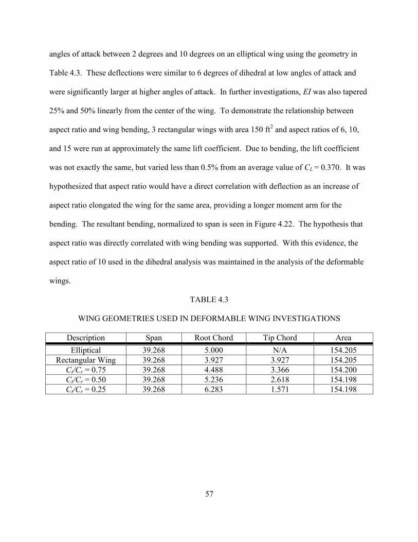
57

angles of attack between 2 degrees and 10 degrees on an elliptical wing using the geometry in

Table 4.3. These deflections were similar to 6 degrees of dihedral at low angles of attack and

were significantly larger at higher angles of attack. In further investigations, EI was also tapered

25% and 50% linearly from the center of the wing. To demonstrate the relationship between

aspect ratio and wing bending, 3 rectangular wings with area 150 ft2 and aspect ratios of 6, 10,

and 15 were run at approximately the same lift coefficient. Due to bending, the lift coefficient

was not exactly the same, but varied less than 0.5% from an average value of CL = 0.370. It was

hypothesized that aspect ratio would have a direct correlation with deflection as an increase of

aspect ratio elongated the wing for the same area, providing a longer moment arm for the

bending. The resultant bending, normalized to span is seen in Figure 4.22. The hypothesis that

aspect ratio was directly correlated with wing bending was supported. With this evidence, the

aspect ratio of 10 used in the dihedral analysis was maintained in the analysis of the deformable

wings.

TABLE 4.3

WING GEOMETRIES USED IN DEFORMABLE WING INVESTIGATIONS

Description Span Root Chord Tip Chord Area Elliptical 39.268 5.000 N/A 154.205

Rectangular Wing 39.268 3.927 3.927 154.205 Ct/Cr = 0.75 39.268 4.488 3.366 154.200 Ct/Cr = 0.50 39.268 5.236 2.618 154.198 Ct/Cr = 0.25 39.268 6.283 1.571 154.198

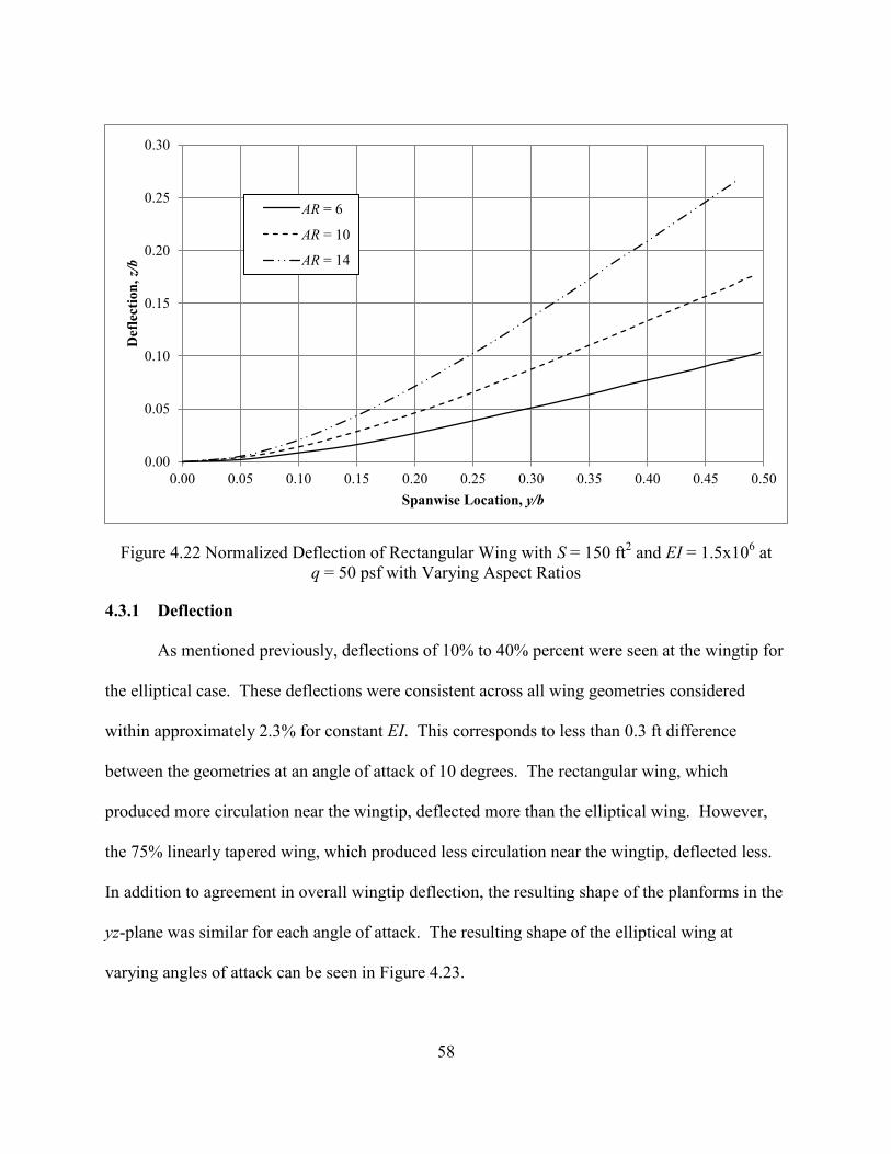
58

Figure 4.22 Normalized Deflection of Rectangular Wing with S = 150 ft2 and EI = 1.5x106 at q = 50 psf with Varying Aspect Ratios

4.3.1 Deflection

As mentioned previously, deflections of 10% to 40% percent were seen at the wingtip for

the elliptical case. These deflections were consistent across all wing geometries considered

within approximately 2.3% for constant EI. This corresponds to less than 0.3 ft difference

between the geometries at an angle of attack of 10 degrees. The rectangular wing, which

produced more circulation near the wingtip, deflected more than the elliptical wing. However,

the 75% linearly tapered wing, which produced less circulation near the wingtip, deflected less.

In addition to agreement in overall wingtip deflection, the resulting shape of the planforms in the

yz-plane was similar for each angle of attack. The resulting shape of the elliptical wing at

varying angles of attack can be seen in Figure 4.23.

0.00

0.05

0.10

0.15

0.20

0.25

0.30

0.00 0.05 0.10 0.15 0.20 0.25 0.30 0.35 0.40 0.45 0.50

Def

lect

ion,

z/b


AR 6

AR 10

AR 15

AR = 6

AR = 10

AR = 14

59

More important than the wingtip deflection distance is the angle at which the wing

deflects. When the circulation over the wing is integrated to find the lift, the contribution that a

panel makes to the overall lift is reduced by . With this in mind, the panel angles were

plotted for the elliptical wing in Figure 4.24. As seen in Figure 4.24, significant bending stops

outboard of 70% semi-span, with the last 30% at roughly the same angle to vertical.

Figure 4.23 Deflection of an Elliptical Wing with EI = 0.15x106 lbf-ft2

The initial angle of attack sweep was helpful for understanding the trends, but was too

coarse for comparing the effect of the various planforms on the deflection. In order to provide a

more isolated comparison of the effect of wing loading on the deflection, data was gathered at

finer angle of attack increments to provide comparisons of wing deflection at constant lift

coefficient.

0.00

0.05

0.10

0.15

0.20

0.25

0.00 0.05 0.10 0.15 0.20 0.25 0.30 0.35 0.40 0.45 0.50

Ver

tical

Loc

atio

n, z/

b


AoA = 2, CL = 0.183

AoA = 4, CL = 0.366

AoA = 6, CL = 0.548

AoA = 8, CL = 0.731

AoA = 10, CL = 0.914

α = 2° CL = 0.183 α = 4° CL = 0.366 α = 6° CL = 0.548 α = 8° CL = 0.731 α = 10° CL = 0.914

60

Figure 4.24 Angle of Local Normal to Vertical for Elliptical Wing with EI = 0.15x106 lbf-ft2

Due to the deformation of the wing, it was not possible to find the angle of attack for a

certain lift-coefficient through interpolation. Instead an iterative process was used to set the

angle of attack such that the wings produced lift coefficients of 0.25, 0.5, and 0.70 with a

tolerance of less than 0.01%.

Figures 4.25 through 4.27 show the spanwise deviation from the elliptical deformation

for each of the planforms at CL = 0.25, 0.50, and 0.70 respectively. From these figures it was

seen that the deviations from the elliptical planform increased as the lift coefficient increased and

that the deviations increased with increasing semi-span location.

Figures 4.28 through 4.30 display the difference from the elliptical wing in local normal

angle for each of the planforms at the previously stated lift coefficients. As can be seen in

Figures 4.28 through 4.30, the difference increased with growing angle of attack, similar to that

seen in Figures 4.25 through 4.27. However the overall percentage difference of panel angle was

0

5

10

15

20

25

30

35

40

0 0.05 0.1 0.15 0.2 0.25 0.3 0.35 0.4 0.45 0.5

Win

g D

efle

ctio

n A

ngle

, ϕ (d

eg)

Wing Fixed Spanwise Location, s/b

AoA = 2 deg, CL = 0.183AoA = 4 deg, CL = 0.366AoA = 6 deg, CL = 0.548AoA = 8 deg, CL = 0.731AoA = 10 deg, CL = 0.914

α = 2° CL = 0.183 α = 4° CL = 0.366 α = 6° CL = 0.548 α = 8° CL = 0.731 α = 10° CL = 0.914

61

slightly larger than that of the panel displacement. Additionally, the deviations in angle

stabilized outboard of 70% semi-span. This indicated that the bending trends seen in the

elliptical wing were the same for all wings, i.e. significant bending occurs on the inboard 70% of

the wing.

To better understand the deviations and their relationship to the spanwise loading of the

wing, the circulation distribution over the wing was examined at all 3 lift coefficients. As the

deflection of the wing increased, the normalized circulation, , decreased away from the

center of the wing, for all planforms. The circulation distribution for CL = 0.7 is presented in

Figure 4.31 and the normalized circulation distribution in Figure 4.32 Most evident in Figure

4.31 is that the 75% linearly tapered wing produces a circulation distribution very similar to that

of a triangular loading, which produces the minimum root bending moment.

Figure 4.25 Deviations from Elliptical Wing Deflection at CL = 0.25 for Wings with EI = 0.15x106 lbf-ft2

-6%

-4%

-2%

0%

2%

4%

6%

0.00 0.05 0.10 0.15 0.20 0.25 0.30 0.35 0.40 0.45 0.50

Diff

eren

ce fr

om E

llipt

ical

Def

lect

ion


Rectangular25% Linearly Tapered50% Linearly Tapered75% Linearly Tapered

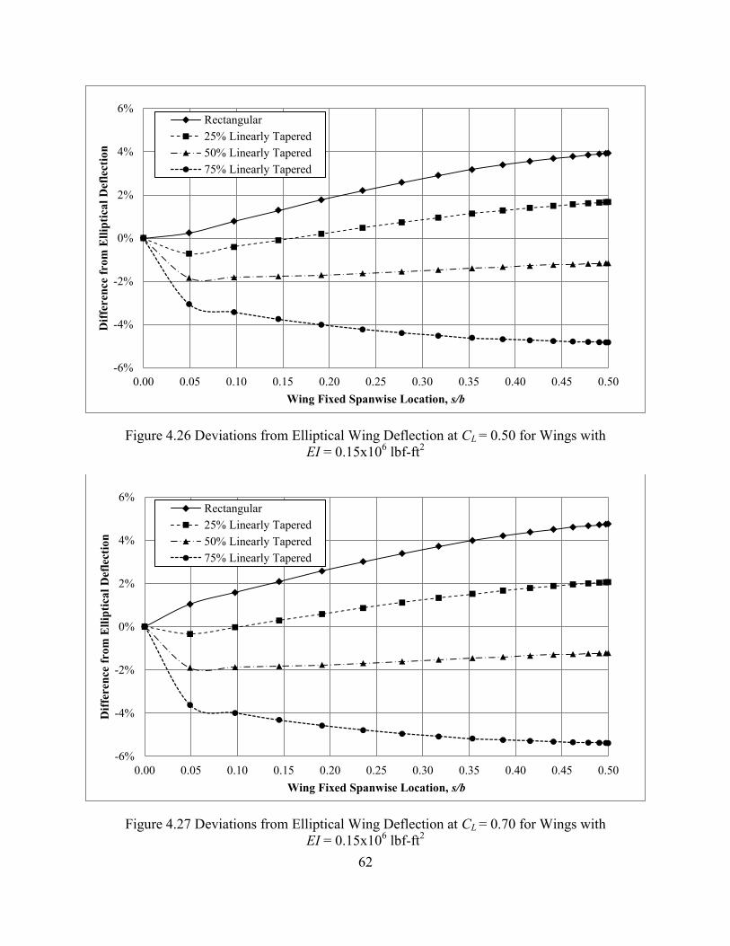
62



-6%

-4%

-2%

0%

2%

4%

6%

0.00 0.05 0.10 0.15 0.20 0.25 0.30 0.35 0.40 0.45 0.50

Diff

eren

ce fr

om E

llipt

ical

Def

lect

ion



-6%

-4%

-2%

0%

2%

4%

6%

0.00 0.05 0.10 0.15 0.20 0.25 0.30 0.35 0.40 0.45 0.50

Diff

eren

ce fr

om E

llipt

ical

Def

lect

ion



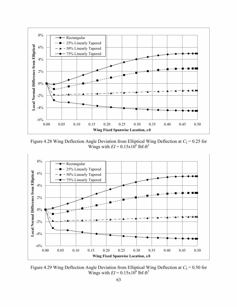
63

Figure 4.28 Wing Deflection Angle Deviation from Elliptical Wing Deflection at CL = 0.25 for Wings with EI = 0.15x106 lbf-ft2


-6%

-4%

-2%

0%

2%

4%

6%

8%

0.00 0.05 0.10 0.15 0.20 0.25 0.30 0.35 0.40 0.45 0.50

Loc

al N

orm

al D

iffer

ence

from

Elli

ptic

al



-6%

-4%

-2%

0%

2%

4%

6%

8%

0.00 0.05 0.10 0.15 0.20 0.25 0.30 0.35 0.40 0.45 0.50

Loc

al N

orm

al D

iffer

ence

from

Elli

ptic

al



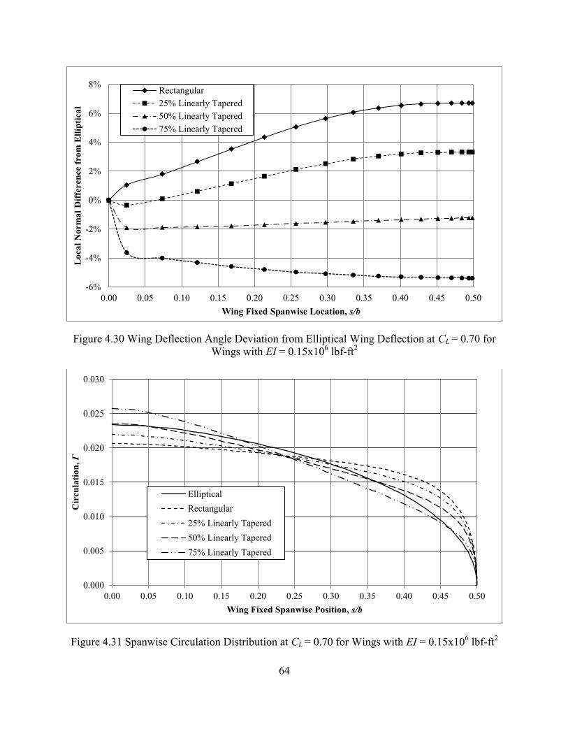
64


Figure 4.31 Spanwise Circulation Distribution at CL = 0.70 for Wings with EI = 0.15x106 lbf-ft2

-6%

-4%

-2%

0%

2%

4%

6%

8%

0.00 0.05 0.10 0.15 0.20 0.25 0.30 0.35 0.40 0.45 0.50

Loc

al N

orm

al D

iffer

ence

from

Elli

ptic

al



0.000

0.005

0.010

0.015

0.020

0.025

0.030

0.00 0.05 0.10 0.15 0.20 0.25 0.30 0.35 0.40 0.45 0.50

Cir

cula

tion,

Γ

Wing Fixed Spanwise Position, s/b

EllipticalRectangular25% Linearly Tapered50% Linearly Tapered75% Linearly Tapered

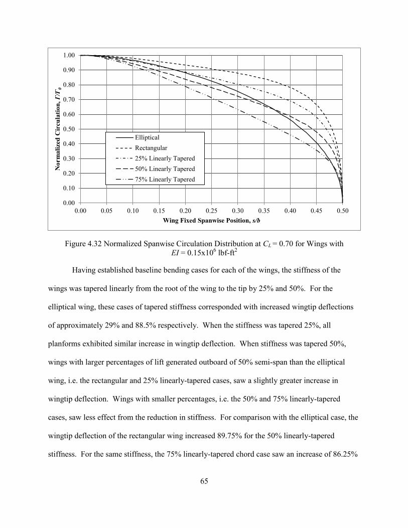
65

Figure 4.32 Normalized Spanwise Circulation Distribution at CL = 0.70 for Wings with EI = 0.15x106 lbf-ft2

Having established baseline bending cases for each of the wings, the stiffness of the

wings was tapered linearly from the root of the wing to the tip by 25% and 50%. For the

elliptical wing, these cases of tapered stiffness corresponded with increased wingtip deflections

of approximately 29% and 88.5% respectively. When the stiffness was tapered 25%, all

planforms exhibited similar increase in wingtip deflection. When stiffness was tapered 50%,

wings with larger percentages of lift generated outboard of 50% semi-span than the elliptical

wing, i.e. the rectangular and 25% linearly-tapered cases, saw a slightly greater increase in

wingtip deflection. Wings with smaller percentages, i.e. the 50% and 75% linearly-tapered

cases, saw less effect from the reduction in stiffness. For comparison with the elliptical case, the

wingtip deflection of the rectangular wing increased 89.75% for the 50% linearly-tapered

stiffness. For the same stiffness, the 75% linearly-tapered chord case saw an increase of 86.25%

0.00

0.10

0.20

0.30

0.40

0.50

0.60

0.70

0.80

0.90

1.00

0.00 0.05 0.10 0.15 0.20 0.25 0.30 0.35 0.40 0.45 0.50

Nor

mal

ized

Cir

cula

tion,

Γ/Γ

0

Wing Fixed Spanwise Position, s/b

EllipticalRectangular25% Linearly Tapered50% Linearly Tapered75% Linearly Tapered

66

The deflections of the elliptical case for varying EI are seen in Figure 4.33. It appeared

that the deflections closer to the wing root showed larger increases than those at the wingtip.

This observation was confirmed by comparing the deflections at the endpoints of each panel to

those seen with constant stiffness. The increase in displacement of the panel endpoints observed

on the elliptical wing is presented in Figure 4.34. The magnitude of the difference in endpoint

deflections as compared to constant flexural rigidity decreased slightly as the distance from the

mid-span increased. The trend seen on the elliptical wing was 5.5% more deflection inboard

than at the wingtips for 25% decrease in stiffness and 7% for a 50% decrease. The same trend

was seen in the other planforms as well, with magnitudes comparable to the elliptical wing.

Figure 4.33 Deflection of Elliptical Wing at CL = 0.5 with Constant and Linearly Tapered Stiffness

0.00

0.05

0.10

0.15

0.20

0.25

0.30

0.00 0.05 0.10 0.15 0.20 0.25 0.30 0.35 0.40 0.45 0.50

Ver

tical

Loc

atio

n, z/

b


Constant EI

25% Linearly Tapered EI


Constant EI



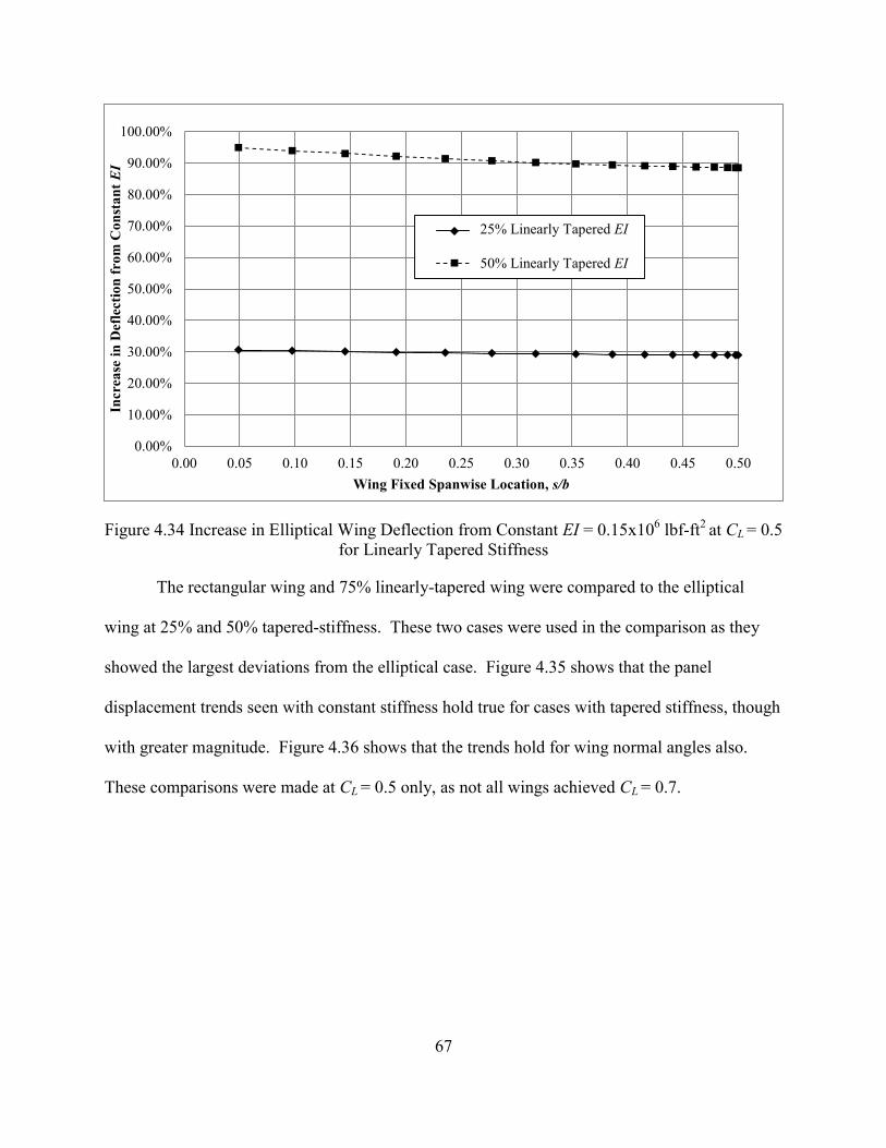
67

Figure 4.34 Increase in Elliptical Wing Deflection from Constant EI = 0.15x106 lbf-ft2 at CL = 0.5 for Linearly Tapered Stiffness

The rectangular wing and 75% linearly-tapered wing were compared to the elliptical

wing at 25% and 50% tapered-stiffness. These two cases were used in the comparison as they

showed the largest deviations from the elliptical case. Figure 4.35 shows that the panel

displacement trends seen with constant stiffness hold true for cases with tapered stiffness, though

with greater magnitude. Figure 4.36 shows that the trends hold for wing normal angles also.

These comparisons were made at CL = 0.5 only, as not all wings achieved CL = 0.7.

0.00%

10.00%

20.00%

30.00%

40.00%

50.00%

60.00%

70.00%

80.00%

90.00%

100.00%

0.00 0.05 0.10 0.15 0.20 0.25 0.30 0.35 0.40 0.45 0.50

Incr

ease

in D

efle

ctio

n fr

om C

onst

ant E

I






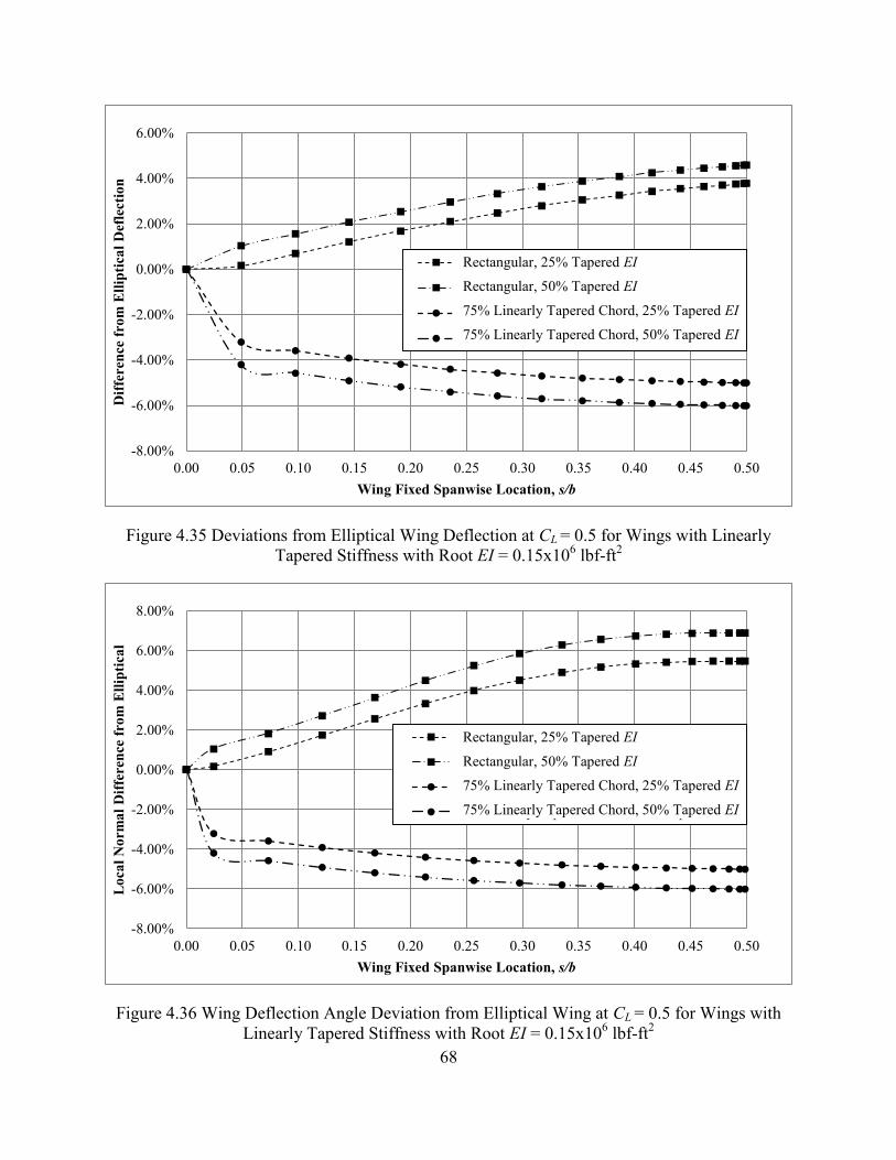
68

Figure 4.35 Deviations from Elliptical Wing Deflection at CL = 0.5 for Wings with Linearly Tapered Stiffness with Root EI = 0.15x106 lbf-ft2

Figure 4.36 Wing Deflection Angle Deviation from Elliptical Wing at CL = 0.5 for Wings with Linearly Tapered Stiffness with Root EI = 0.15x106 lbf-ft2

-8.00%

-6.00%

-4.00%

-2.00%

0.00%

2.00%

4.00%

6.00%

0.00 0.05 0.10 0.15 0.20 0.25 0.30 0.35 0.40 0.45 0.50

Diff

eren

ce fr

om E

llipt

ical

Def

lect

ion


Rectangular, 25% Tapered EI


75% Linearly Tapered Chord, 25% Tapered EI


-8.00%

-6.00%

-4.00%

-2.00%

0.00%

2.00%

4.00%

6.00%

8.00%

0.00 0.05 0.10 0.15 0.20 0.25 0.30 0.35 0.40 0.45 0.50

Loc

al N

orm

al D

iffer

ence

from

Elli

ptic

al






Rectangular, 25% Tapered EI Rectangular, 50% Tapered EI

75% Linearly Tapered Chord, 25% Tapered EI 75% Linearly Tapered Chord, 50% Tapered EI


Rectangular, 50% Tapered EI 75% Linearly Tapered Chord, 25% Tapered EI


69

4.3.2 Effects on Lift Coefficient and Span Efficiency Factor

Section 4.2 provided insight into lift and drag penalties due to small dihedral angles on

the wing. These penalties were approximately 3% at for both lift and span efficiency

factor. Additionally, these penalties were independent of angle of attack when the wing had no

twist. When the rigid geometry was replaced with a deformable wing, the deflections seen were

significantly larger and resulted in lift and drag penalties that were dependent on angle of attack.

At higher angles of attack, the penalties were greater than those for rigid wings.

As can be seen in Figure 4.37 (a), the lift coefficient penalty due to the deformation for

the elliptical wing was 0.4% for constant stiffness at , but 10.1% at . Similarly,

from Figure 4.36 (b), the span efficiency factor penalty was only 0.1% for and 3.6% at

. For the cases of tapered stiffness, the ultimate penalty in lift coefficient increased

significantly, while the penalty at remained less than 1.2%; the penalty in span efficiency

factor was only 0.4% at and 22.7% at .

An interesting artifact of the deflection was the quasi-stall created for wings with 50%

linearly-tapered stiffness, seen in Figure 4.37 (a) for the elliptical wing. This feature was present

for all planforms at an angle of attack of 10 degrees.

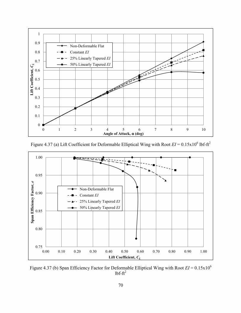
70

Figure 4.37 (a) Lift Coefficient for Deformable Elliptical Wing with Root EI = 0.15x106 lbf-ft2

Figure 4.37 (b) Span Efficiency Factor for Deformable Elliptical Wing with Root EI = 0.15x106 lbf-ft2

0

0.1

0.2

0.3

0.4

0.5

0.6

0.7

0.8

0.9

1

0 1 2 3 4 5 6 7 8 9 10

Lift

Coe

ffic

ient

, CL


Non-Deformable FlatConstant EI25% Tapered EI50% Tapered EI

0.75

0.80

0.85

0.90

0.95

1.00

0.00 0.10 0.20 0.30 0.40 0.50 0.60 0.70 0.80 0.90 1.00

Span

Eff

icie

ncy

Fact

or, e


Non-Deformable FlatConstant EI25% Tapered EI50% Tapered EI

Non-Deformable Flat Constant EI 25% Linearly Tapered EI 50% Linearly Tapered EI

Non-Deformable Flat Constant EI 25% Linearly Tapered EI 50% Linearly Tapered EI

71

The penalty in lift coefficient for each of the planforms was similar, with approximately

10% lift loss at for constant stiffness and 37% loss for the 50% tapered case. Figure

4.38 shows the lift loss for each planform compared to a flat wing of the same geometry. Part (a)

of Figure 4.38 shows the case of constant stiffness, part (b) shows the case of 25% linearly-

tapered stiffness, and part (c) shows the case of 50% linearly-tapered stiffness. The reason for

the exaggerated effect on the 75% tapered chord case was not understood, but there was no

reason to disregard these results.

In all cases the deflection of the wing decreased the span efficiency factor. However, flat

planforms that generated lift further outboard, when compared to an elliptical wing, experienced

a smaller penalty.

Figure 4.38 (a) Decrease in Lift Coefficient Due to Wing Deflection for Constant EI = 0.15x106 lbf-ft2

-14%

-12%

-10%

-8%

-6%

-4%

-2%

0%

0 1 2 3 4 5 6 7 8 9 10

Dec

reas

e in

Lift

Coe

ffic

ient


Elliptical

Rectangular

25% Linearly Tapered



72

Figure 4.38 (b) Decrease in Lift Coefficient Due to Wing Deflection for 25% Linearly-Tapered Stiffness with Root EI = 0.15x106 lbf-ft2

Figure 4.38 (c) Decrease in Lift Coefficient Due to Wing Deflection for 50% Linearly-Tapered Stiffness with Root EI = 0.15x106 lbf-ft2

-20%

-18%

-16%

-14%

-12%

-10%

-8%

-6%

-4%

-2%

0%

0 1 2 3 4 5 6 7 8 9 10

Dec

reas

e in

Lift

Coe

ffic

ient


Elliptical

Rectangular




-40%

-35%

-30%

-25%

-20%

-15%

-10%

-5%

0%

0 1 2 3 4 5 6 7 8 9 10

Dec

reas

e in

Lift

Coe

ffic

ient


Elliptical

Rectangular




73

This decrease in the effect on span efficiency factor was due to an effective twist in the

wing. If at a local position on the wing the deflection angle was , then the effective angle of

attack would be:

(4.6)

which would cause an effective twist angle in the model of:

( ) (4.7)

At low angles of attack, the deflection angles were relatively small, thereby minimizing the

effective twist in the model. As the angle of attack increased or the stiffness of the wing

decreased, the twist increased. The increased twist led to a reduction in circulation generated

near the wingtips. The reduction in circulation near the wingtips improved the shape of the

distribution for planforms that produced a greater percentage of lift nearer the wingtips as

compared to an elliptical wing. For a flat wing, this washout increased the span efficiency

factor. Due to the deformation, not all the force generated normal to the wing created lift, even

though it still created drag. This resulted in decreasing the span efficiency factor more than was

gained by the improvement of the circulation distribution.

The decrease in span efficiency factor for the various cases is seen in Figure 4.39. Part

(a) of Figure 4.39 shows the case of constant stiffness, part (b) shows the case of 25% linearly-

tapered stiffness, and part (c) shows the case of 50% linearly-tapered stiffness. As can be seen,

the elliptical case experienced the most significant decrease in span efficiency factor; the

rectangular wing experienced the least.

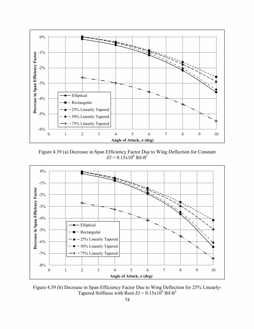
74

Figure 4.39 (a) Decrease in Span Efficiency Factor Due to Wing Deflection for Constant EI = 0.15x106 lbf-ft2

Figure 4.39 (b) Decrease in Span Efficiency Factor Due to Wing Deflection for 25% Linearly-Tapered Stiffness with Root EI = 0.15x106 lbf-ft2

-6%

-5%

-4%

-3%

-2%

-1%

0%

0 1 2 3 4 5 6 7 8 9 10

Dec

reas

e in

Spa

n E

ffic

ienc

y Fa

ctor


Elliptical

Rectangular




-8%

-7%

-6%

-5%

-4%

-3%

-2%

-1%

0%

0 1 2 3 4 5 6 7 8 9 10

Dec

reas

e in

Spa

n E

ffic

ienc

y Fa

ctor


Elliptical

Rectangular




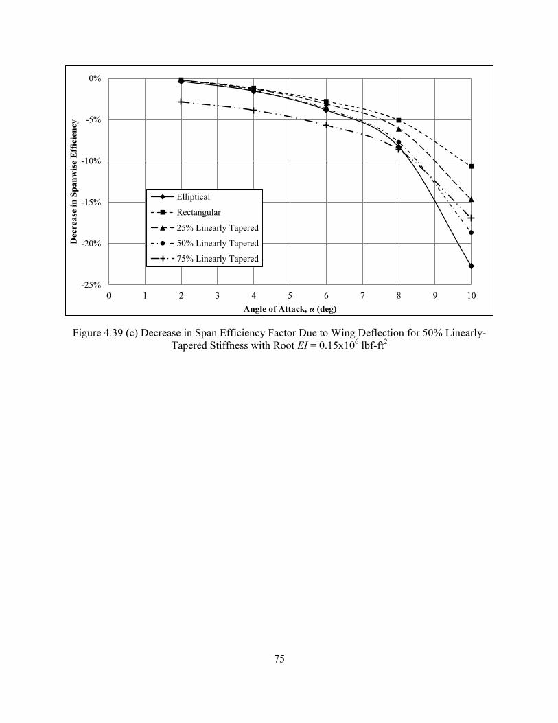
75

Figure 4.39 (c) Decrease in Span Efficiency Factor Due to Wing Deflection for 50% Linearly-Tapered Stiffness with Root EI = 0.15x106 lbf-ft2

-25%

-20%

-15%

-10%

-5%

0%

0 1 2 3 4 5 6 7 8 9 10

Dec

reas

e in

Spa

nwis

e E

ffic

ienc

y


Elliptical

Rectangular




76

CHAPTER 5

SUMMARY AND CONCLUSION

The research presented in this thesis can be summarized as follows. In Chapter 1, a

review of the technical literature relating to lifting-line theory and the modifications to the

original formulation was presented. This information showed that while many modifications

have been made to the original formulation, little work has been published on non-planar

applications of the theory. The technical literature that did address non-planar wings focused

primarily on the optimum circulation distribution, disregarding the planform shape required to

produce the distribution.

Chapter 2 discussed the traditional formulation of Prandtl’s lifting-line theory in detail.

The theory assumed that a bound vortex was attached at the quarter chord, with an infinite

number of trailing vortex filaments of infinitesimal strength forming the wake. The optimal

circulation distribution was shown to be elliptical. The solution for a general planform using a

Fourier series for the circulation was demonstrated and the analytical solution for the influence

of the wake provided.

Starting from the original formulation, Chapter 3 provided an expansion to lifting-line

theory. Only 2 changes were made to the assumptions for the original theory. First, instead of

considering a planar wake, the wake was assumed to remain in the same shape as the wing and

not roll up or sink. Secondly, the induced velocity from the bound vortex was considered to

have no self-induced velocities, despite being non-planar. These new assumptions led to an

expanded governing equation for lifting-line theory. This expanded form simplified to the

traditional formulation for planar wings. Using geometry specific to wings with dihedral, the

new formulation was simplified to a more compact form for solving. A simplified finite element

77

method was presented which considered bending in one direction over a beam. This method was

coupled with the generalized form of the theory to form a static aeroelastic model for the wing.

The results for a rigid wing with dihedral and a deformable wing were presented in

Chapter 4. A convergence analysis performed showed satisfactory convergence of the Fourier

coefficients toward their respective asymptotic values using 32 panels over the wing. Analysis

of a wing with dihedral showed the trends of increasing aspect ratio to be independent of

dihedral angle. An increase of aspect ratio decreased induced drag and increased lift-curve slope

the same percentage for flat wings and wings with dihedral. Furthermore, an elliptical wing

produced the minimum induced drag for both flat wings and wings with dihedral. Dihedral

decreased the efficiency of all untwisted wings equally. The decrease in span efficiency factor

and lift-curve slope for dihedral angles less than 6 degrees was less than 1.1% compared with flat

wings.

The deflection seen in the deformable wing was similar for all planforms investigated.

Compared to the elliptical wing, all other planforms showed deflections within ±6%. Planforms

with more lift generated toward the wingtips experienced larger deflections than those with more

lift generated closer to the center of the wing. Significant bending of the wing occurred within

75% semi-span for all planforms. The taper of EI along the wing increased deflection of the

wing 30% and 90% for cases of 25% and 50% linearly tapered EI respectively.

Deformation of the wing caused a non-linear decrease in lift coefficient and span

efficiency factor, most noticeable in the 50% tapered stiffness. At low angles of attack, the lift

coefficient penalty was less than 1%, but increased to 10% at 10 degrees angle of attack.

Similarly the span efficiency factor showed less than 0.2% decrease at 2 degrees angle of attack,

but more than 3% decrease at 10 degrees. The elliptical wing showed the most significant

78

decrease in span efficiency factor due to deflection and the rectangular wing showed the least.

These effects were due to the effective twist non-planar wings experience at non-zero angles of

attack.

To more fully understand the effect of non-planar geometries on the aerodynamics of a

wing, additional work on the model is recommended, primarily focused on the addition of a term

to account for the self-induced velocities of the bound vortex.

79

REFERENCES

80

REFERENCES

[1] Prandtl, L., “Applications of Modern Hydrodynamics to Aeronautics,” NACA TR-116, June 1921.

[2] Munk, M., “The Minimum Induced Drag of Aerofoils,” NACA Report 121, 1923.

[3] Glauert, H., “The Monoplane Aerofoil,” The Elements of Airfoil and Airscrew Theory, Cambridge Univ. Press, Cambridge, UK, 1926, pp. 137-155.

[4] Anderson, J. Jr., “Incompressible Flow over Finite Wings,” Fundamentals of Aerodynamics, 4th ed., McGraw-Hill, New York, NY, 2005, pp. 391-465.

[5] Katz, J. and Plotkin, A., “Three-Dimensional Small-Disturbance Solutions,” Low-Speed Aerodynamics, 2nd ed., Cambridge Univ. Press, New York, NY, 2001, pp. 167-205.

[6] Rasmussen, M. and Smith, D., “Lifting-Line Theory for Arbitrarily Shaped Wings,” Journal of Aircraft, Vol. 36, No. 2, 1999, pp. 340-348.

[7] Gates, S., “An Analysis of Rectangular Monoplane with Hinged Tips,” Reports and Memoranda 1175, Aeronautical Research Committee, Aeronautical Research Council, London, 1928.

[8] Anderson, R and Millsaps, K., “Application of the Galerkin Method to the Prandtl Lifting-Line Equation,” Journal of Aircraft, Vol. 1, No. 3, 1964, pp. 126-128.

[9] Karamcheti, Krishnamurty, “Elements of Thin Airfoil Theory” and “Elements of Finite Wing Theory,” Principles of Ideal-Fluid Aerodynamics, John Wiley & Sons, Inc., New York, 1966, p. 510 and p. 535 – 567.

[10] Lotz, I., “Berechnung der Auftriebsverteilug beliebig geformter Flugel,” Zeitschrift für Flugetechnik und Motorluftschiffahrt, Vol. 22, No. 7, 1931, pp. 189-195.

[11] Weissinger, J., “The Lift Distribution of Swept-Back Wings,” NACA TM-1120, March 1947.

[12] Pistolesi, E., “Considerazioni sul problema del biplane,” Aerotecnica., Vol. 13, pp. 185, 1933.

[13] Owens, D. B., “Weissinger’s Model of the Nonlinear Lifting-Line Method for Aircraft Design,” 36th AIAA Aerospace Sciences Meeting and Exhibit, American Institute for Aeronautics and Astronautics, 1998.

81

REFERENCES

[14] Cone, C., “The Theory of Induced Lift and Minimum Induced Drag of Nonplanar Lifting Systems,” NASA TR R-139, 1962.

[15] Takahashi, T. and Donovan, S., “Non Planar Span Loads for Minimum Induced Drag,” 49th AIAA Aerospace Sciences Meeting, Orlando, Florida, January 2011, American Institute for Aeronautics and Astronautics, 2011.

[16] Nguyen, N., “Elastically Shaped Future Air Vehicle Concept,” NASA Innovation Fund 2010 Project, October 2010.

[17] Tietjens, O and Prandtl, J, “Airfoil Theory,” Hydro- & Aero-mechanics, Dover, New York, 1957, p. 185 – 225.

[18] McCormick, Barnes, “Drag,” Aerodynamics, Aeronautics, and Flight Mechanics, 1st ed., John Wiley & Sons, New York, 1979, p. 186-195.

[19] Bridges, David H., “Finite Wing Lift-Curve Slope Calculations using Lifting-Line Theory,” AIAA Applied Aerodynamics Conference, AIAA Paper 2005-4839, June 2005.

82

APPENDIX

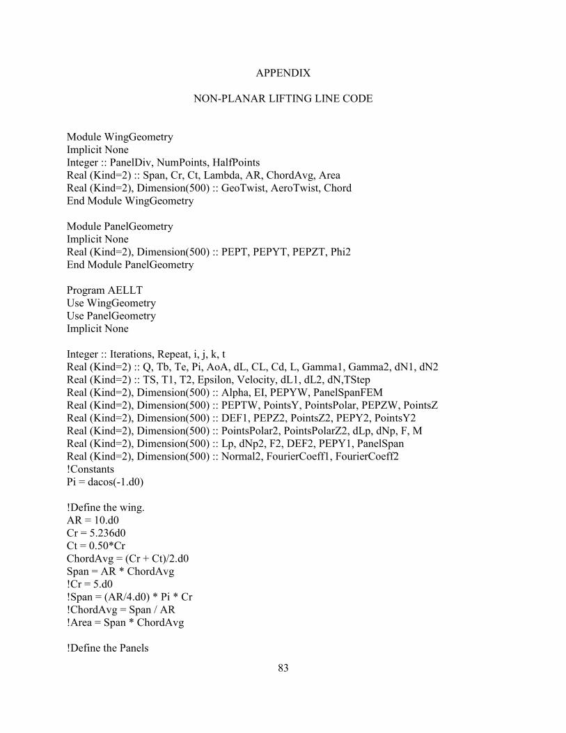
83

APPENDIX

NON-PLANAR LIFTING LINE CODE

Module WingGeometry Implicit None Integer :: PanelDiv, NumPoints, HalfPoints Real (Kind=2) :: Span, Cr, Ct, Lambda, AR, ChordAvg, Area Real (Kind=2), Dimension(500) :: GeoTwist, AeroTwist, Chord End Module WingGeometry Module PanelGeometry Implicit None Real (Kind=2), Dimension(500) :: PEPT, PEPYT, PEPZT, Phi2 End Module PanelGeometry Program AELLT Use WingGeometry Use PanelGeometry Implicit None Integer :: Iterations, Repeat, i, j, k, t Real (Kind=2) :: Q, Tb, Te, Pi, AoA, dL, CL, Cd, L, Gamma1, Gamma2, dN1, dN2 Real (Kind=2) :: TS, T1, T2, Epsilon, Velocity, dL1, dL2, dN,TStep Real (Kind=2), Dimension(500) :: Alpha, EI, PEPYW, PanelSpanFEM Real (Kind=2), Dimension(500) :: PEPTW, PointsY, PointsPolar, PEPZW, PointsZ Real (Kind=2), Dimension(500) :: DEF1, PEPZ2, PointsZ2, PEPY2, PointsY2 Real (Kind=2), Dimension(500) :: PointsPolar2, PointsPolarZ2, dLp, dNp, F, M Real (Kind=2), Dimension(500) :: Lp, dNp2, F2, DEF2, PEPY1, PanelSpan Real (Kind=2), Dimension(500) :: Normal2, FourierCoeff1, FourierCoeff2 !Constants Pi = dacos(-1.d0) !Define the wing. AR = 10.d0 Cr = 5.236d0 Ct = 0.50*Cr ChordAvg = (Cr + Ct)/2.d0 Span = AR * ChordAvg !Cr = 5.d0 !Span = (AR/4.d0) * Pi * Cr !ChordAvg = Span / AR !Area = Span * ChordAvg !Define the Panels

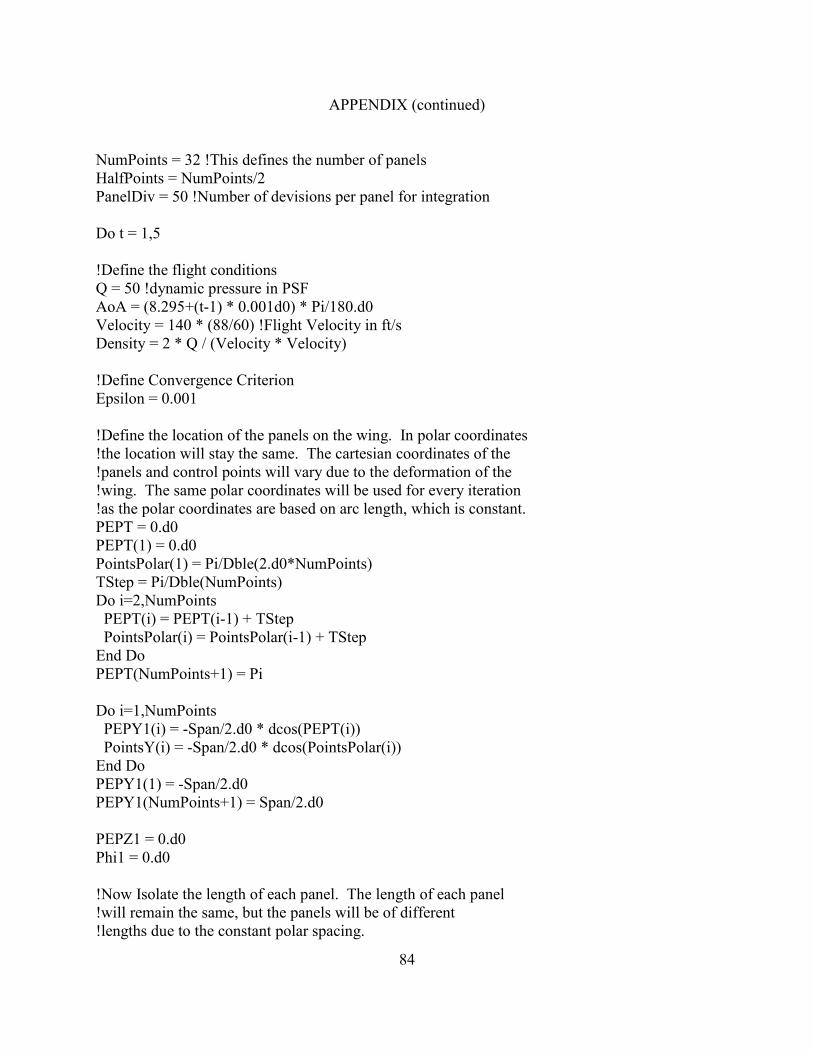
84

APPENDIX (continued)

NumPoints = 32 !This defines the number of panels HalfPoints = NumPoints/2 PanelDiv = 50 !Number of devisions per panel for integration Do t = 1,5 !Define the flight conditions Q = 50 !dynamic pressure in PSF AoA = (8.295+(t-1) * 0.001d0) * Pi/180.d0 Velocity = 140 * (88/60) !Flight Velocity in ft/s Density = 2 * Q / (Velocity * Velocity) !Define Convergence Criterion Epsilon = 0.001 !Define the location of the panels on the wing. In polar coordinates !the location will stay the same. The cartesian coordinates of the !panels and control points will vary due to the deformation of the !wing. The same polar coordinates will be used for every iteration !as the polar coordinates are based on arc length, which is constant. PEPT = 0.d0 PEPT(1) = 0.d0 PointsPolar(1) = Pi/Dble(2.d0*NumPoints) TStep = Pi/Dble(NumPoints) Do i=2,NumPoints PEPT(i) = PEPT(i-1) + TStep PointsPolar(i) = PointsPolar(i-1) + TStep End Do PEPT(NumPoints+1) = Pi Do i=1,NumPoints PEPY1(i) = -Span/2.d0 * dcos(PEPT(i)) PointsY(i) = -Span/2.d0 * dcos(PointsPolar(i)) End Do PEPY1(1) = -Span/2.d0 PEPY1(NumPoints+1) = Span/2.d0 PEPZ1 = 0.d0 Phi1 = 0.d0 !Now Isolate the length of each panel. The length of each panel !will remain the same, but the panels will be of different !lengths due to the constant polar spacing.

85


Do i=1,NumPoints PanelSpan(i) = PEPY1(i+1) - PEPY1(i) End Do Do i=1,HalfPoints PanelSpanFEM(i) = PanelSpan(HalfPoints+i) End Do !We can now define the angle of attack and local chord !for the control points. Do i = 1, NumPoints GeoTwist(i) = 0.d0 !Geometric twist in RADIANS AeroTwist(i) = 0.d0 * (Pi/180.d0) !Alpha_L=0 in RADIANS Alpha(i) = AoA + GeoTwist(i) - AeroTwist(i) !Local AoA in RADIANS Chord(i) = Cr + (abs(PointsY(i))/(Span/2.d0)) * (Ct-Cr) !Chord(i) = 2 * ((Cr/2.d0)**2 * (1 - (2.d0 * PointsY(i) / Span)**2))**0.5 End Do !Define the Structural Properties of the wing Do i =HalfPoints + 1,NumPoints EI(i) = .15d0 * 10**6 !- (0.5d0 * (0.15d0*10**6) * abs(PointsY(i))/(Span/2.d0)) !Structural strength, half wing EI(NumPoints-(i-1)) = EI(i) End Do !The wing is still flat - use the analytical solution. Call TLLM(PointsPolar, Alpha, FourierCoeff1) !Calculate the normal force for use in the FEM model. Tb = PEPT(HalfPoints+1) Te = PEPT(HalfPoints+2) TS = (Te-Tb) / 100 dCLp = 0.d0 dLp = 0.d0 Do i=HalfPoints+1,NumPoints T1 = Tb T2 = Tb + TS Do j=1,100

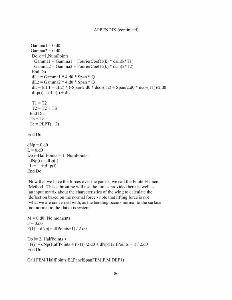
86


Gamma1 = 0.d0 Gamma2 = 0.d0 Do k =1,NumPoints Gamma1 = Gamma1 + FourierCoeff1(k) * dsin(k*T1) Gamma2 = Gamma2 + FourierCoeff1(k) * dsin(k*T2) End Do dL1 = Gamma1 * 4.d0 * Span * Q dL2 = Gamma2 * 4.d0 * Span * Q dL = (dL1 + dL2) * (-Span/2.d0 * dcos(T2) + Span/2.d0 * dcos(T1))/2.d0 dLp(i) = dLp(i) + dL T1 = T2 T2 = T2 + TS End Do Tb = Te Te = PEPT(i+2) End Do dNp = 0.d0 L = 0.d0 Do i=HalfPoints + 1, NumPoints dNp(i) = dLp(i) L = L + dLp(i) End Do !Now that we have the forces over the panels, we call the Finite Element !Method. This subroutine will use the forces provided here as well as !an input matrix about the characteristics of the wing to calculate the !deflection based on the normal force - note that lifting force is not !what we are concerned with, as the bending occurs normal to the surface !not normal to the flat axis system M = 0.d0 !No moments F = 0.d0 F(1) = dNp(HalfPoints+1) / 2.d0 Do i= 2, HalfPoints + 1 F(i) = dNp(HalfPoints + (i-1)) /2.d0 + dNp(HalfPoints + i) / 2.d0 End Do Call FEM(HalfPoints,EI,PanelSpanFEM,F,M,DEF1)

87


Open(10,File='F:\AeroEng Stuff\Data Output\LT50_UntaperedEI_SF.dat') Write(10,*) '****************************************************************************' Write(10,10) Write(10,11) (FourierCoeff1(i),i = 1, NumPoints) Write(10,11) (DEF1(i),i = 1, HalfPoints) !The deflection is defined by the FEM. Now we must relate this to !the entire wing. The deflection will then also define the location !in the y-direction as well, as the wing does not change length !only bends. Do Iterations = 1,1000 Do i=HalfPoints+2,NumPoints+1 PEPZ2(i) = DEF1(i-(HalfPoints+1)) End Do Do i=1,HalfPoints PEPZ2(i) = PEPZ2((NumPoints+1) - (i-1)) End Do PEPZ2(HalfPoints+1) = 0.d0 Do i=1,NumPoints Phi2(i) = dasin((PEPZ2(i+1)-PEPZ2(i))/PanelSpan(i)) End Do PEPY2= 0.d0 Do i=HalfPoints+2,NumPoints PEPY2(i) = PEPY2(i-1) + PanelSpan(i-1) * dcos(Phi2(i)) End Do PEPY2(NumPoints+1) = Span/2.d0 Do i=1,HalfPoints PEPY2(i) = -PEPY2((NumPoints+1)-(i-1)) End Do Do i=1,NumPoints Normal2(i) = AoA * dcos(Phi2(i)) + GeoTwist(i) - AeroTwist(i) End Do PEPYT = 0.d0 PEPZT = 0.d0

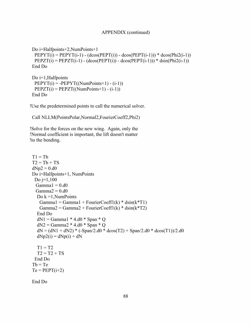
88


Do i=Halfpoints+2,NumPoints+1 PEPYT(i) = PEPYT(i-1) - (dcos(PEPT(i)) - dcos(PEPT(i-1))) * dcos(Phi2(i-1)) PEPZT(i) = PEPZT(i-1) - (dcos(PEPT(i)) - dcos(PEPT(i-1))) * dsin(Phi2(i-1)) End Do Do i=1,Halfpoints PEPYT(i) = -PEPYT((NumPoints+1) - (i-1)) PEPZT(i) = PEPZT((NumPoints+1) - (i-1)) End Do !Use the predetermined points to call the numerical solver. Call NLLM(PointsPolar,Normal2,FourierCoeff2,Phi2) !Solve for the forces on the new wing. Again, only the !Normal coefficient is important, the lift doesn't matter !to the bending. T1 = Tb T2 = Tb + TS dNp2 = 0.d0 Do i=Halfpoints+1, NumPoints Do j=1,100 Gamma1 = 0.d0 Gamma2 = 0.d0 Do k =1,NumPoints Gamma1 = Gamma1 + FourierCoeff1(k) * dsin(k*T1) Gamma2 = Gamma2 + FourierCoeff1(k) * dsin(k*T2) End Do dN1 = Gamma1 * 4.d0 * Span * Q dN2 = Gamma2 * 4.d0 * Span * Q dN = (dN1 + dN2) * (-Span/2.d0 * dcos(T2) + Span/2.d0 * dcos(T1))/2.d0 dNp2(i) = dNp(i) + dN T1 = T2 T2 = T2 + TS End Do Tb = Te Te = PEPT(i+2) End Do

89


F2 = 0.d0 F2(1) = dNp2(HalfPoints+1) / 2.d0 Do i= 2, HalfPoints + 1 F2(i) = dNp2(HalfPoints + (i-1)) /2.d0 + dNp2(HalfPoints + i) / 2.d0 End Do !Call the bending model to solve the new shape Call FEM(HalfPoints,EI,PanelSpanFEM,F2,M,DEF2) Write(10,12) Iterations Write(10,11) (FourierCoeff2(i),i = 1, NumPoints) Write(10,11) (DEF2(i),i = 1, HalfPoints) Repeat = 0 !Compare the deflections. Converged solutions are within espilon. !If the solution is not converged, iterate again. Do i=1,HalfPoints+1 If(abs(DEF1(i) - DEF2(i)) .gt. Epsilon) Repeat = 1 If(abs(DEF1(i) - DEF2(i)) .gt. Epsilon) Exit End Do !Exit the loop if the solution has converged If(Repeat .eq. 0) Exit !Move the necessary values to a different storage location DEF1 = DEF2 F1 = F2 dNp1 = dNp2 Phi1 = Phi2 Normal1 = Normal2 FourierCoeff1 = FourierCoeff2 End Do If(Repeat .ne. 0) Write(*,*)'Unconverged Solution' If(Repeat .ne. 0) Pause L = 0.d0 Do i=Halfpoints+1, NumPoints Lp(i) = dNp(i) * dcos(Phi2(i))

90


L = L + Lp(i) End Do !Only half the wing calculated, double to get correct lift L = 2.d0 * L !Compute Lift Coefficient Cl = L / (Q * ChordAvg * Span) Cd = 0.d0 Do i=1,NumPoints-1,2 Cd = Cd + (pi * AR) * Dble(i) * FourierCoeff2(i) * FourierCoeff2(i) End Do Write(10,13) (AoA*180.d0/Pi),Cl,Cd End Do Close(10) 10 Format('Analytical Solution for:') 11 Format(32(F15.12,1x)) 12 Format('Iteration: ',I4) 13 Format('AoA: ',F8.5,1x,'Cl= ',F8.7,1x, 'Cd= ', F8.7) End Program AELLT Subroutine TLLM(PointsPolar, Alpha, FourierCoeff) Use WingGeometry Implicit None Integer :: i, j, Status Integer, Dimension(500) :: P Integer, Parameter :: Size = 500 Real (Kind=2), Dimension(500,500) :: LLMatrix Real (Kind=2), Dimension(500) :: PointsPolar, FourierCoeff, Alpha Real (Kind=2) :: Pi, Geo, Ind Pi = dacos(-1.d0) !Create the influence matrix Do i = 1, NumPoints Do j = 1, NumPoints Geo = 0.d0

91


Ind = 0.d0 LLMatrix(i,j) = 0.d0 Geo = dsin(Dble(j)*PointsPolar(i)) * (2*Span)/(Pi*Chord(i)) Ind = Dble(j) * dsin(Dble(j)*PointsPolar(i))/dsin(PointsPolar(i)) LLMatrix(i,j) = Geo + Ind End Do End Do Open(Unit = 1, File = 'InfluenceMatrixT.csv') Write(1,10) ((LLMatrix(i,j),j = 1, NumPoints),i = 1, NumPoints) Close(1) Call GAUSSP(Size, NumPoints, LLMatrix, Alpha, Status, FourierCoeff, P) If (Status .eq. 1) Write(*,*) 'Failure in solution of the circulation distribution' 10 Format(32(F11.7,1x)) End Subroutine TLLM Subroutine NLLM(PointsPolar,Normal,FourierCoeff,Phi2) Use WingGeometry Implicit None Integer :: i, j, Status Integer, Dimension(500) :: P Integer, Parameter :: Size = 500 Real (Kind=2), Dimension(500,500) :: LLMatrix Real (Kind=2), Dimension(500) :: PointsPolar, FourierCoeff, Normal,Phi2, Phi Real (Kind=2) :: Pi, T0, Y0, Z0, Sum, PhiP Pi = dacos(-1.d0) !Create the influence matrix. Do i = 1, NumPoints PhiP = Phi2(i) Do j = 1, NumPoints T0 = PointsPolar(i) Sum = 0.d0 Call NumericalInfluence(PointsPolar,T0,PhiP,i,j,Sum) LLMatrix(i,j) = Sum + (dsin(Dble(j)*T0) * (2*Span)/(Pi*Chord(i))) End Do End Do

92


!Now solve the set of simultaneous equations developed. Open(Unit = 1, File = 'InfluenceMatrixN.csv') Write(1,10) ((LLMatrix(i,j),j = 1, NumPoints),i = 1, NumPoints) Close(1) Call GAUSSP (Size, NumPoints, LLMatrix, Normal, Status, FourierCoeff, P) If (Status .eq. 1) Write(*,*) 'Failure in solution of the circulation distribution' 10 Format(32(F11.7,1x)) End Subroutine NLLM Subroutine NumericalInfluence(PointsPolar,T0,PhiP,i,j,Sum) Use WingGeometry Implicit None Real (Kind=2) :: Pi, Step, T1, Sum, T2, T3, I1, I2, I3, Int, T0, CTL1, CTL2, PhiP Real (Kind=2), Dimension(500) :: PointsPolar Integer :: SD, Pts, k, i, j, LLP, ULP, SubPts Pi = dacos(-1.d0) SubPts = 50 !EVEN Step = PointsPolar(1)/(Dble(SubPts/2)) T1 = 0.d0 Sum = 0.d0 LLP = (i-1) * SubPts + SubPts/2 ULP = (NumPoints * SubPts) - LLP Do k=1,LLP-1,1 T3 = T1 + Step T2 = T1 + Step/2.d0 Call Influence(I1,j,T0,T1,PhiP) Call Influence(I2,j,T0,T2,PhiP) Call Influence(I3,j,T0,T3,PhiP) Sum = Sum + Step/6.d0 * (I1 + 4.d0 * I2 + I3) T1 = T1 + Step End Do T1=T1 + 2*Step

93


Do k=1,ULP-1,1 T3 = T1 + Step T2 = T1 + Step/2.d0 Call Influence(I1,j,T0,T1,PhiP) Call Influence(I2,j,T0,T2,PhiP) Call Influence(I3,j,T0,T3,PhiP) Sum = Sum + Step/6.d0 * (I1 + 4.d0 * I2 + I3) T1 = T1 + Step End Do !Integrate across the discontinuity. T1 = T0 - Step T2 = T0 + Step Call Influence(I1,j,T0,T1,PhiP) Call Influence(I2,j,T0,T2,PhiP) Int = Step * (I1 + I2) Sum = Sum + Int !Divide the sum by Pi, as found in the formulation. Sum = Sum/Pi End Subroutine NumericalInfluence !Calculate the influence integrand at each theta location. Subroutine Influence(Int,j,T0,T,PhiP) Use WingGeometry Implicit None Real (Kind=2) :: T,T0,Y,Y0,Z,Z0,FH,FL,FC,Int,Pi,Mult,PhiP Integer :: i, j Pi = dacos(-1.d0) FH = Dble(j) * dcos(dble(j) * T) Call CartLoc(T,Y,Z) Call CartLoc(T0,Y0,Z0) FL = ((Z0-Z)**2 + (Y0-Y)**2)**0.5

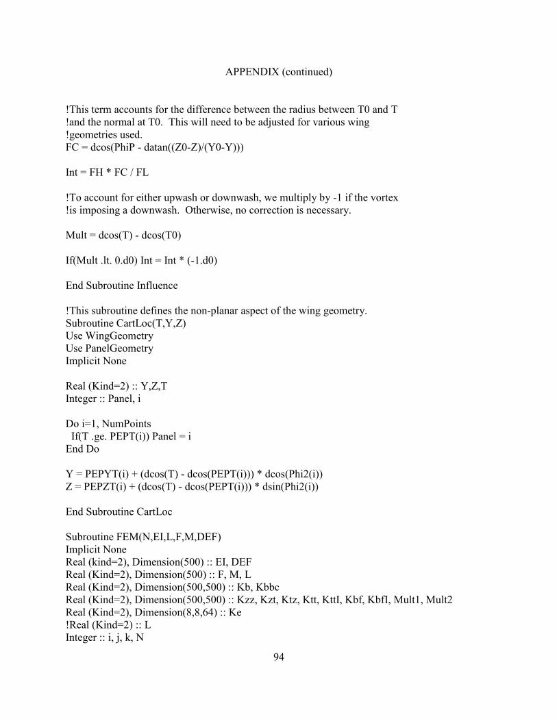
94


!This term accounts for the difference between the radius between T0 and T !and the normal at T0. This will need to be adjusted for various wing !geometries used. FC = dcos(PhiP - datan((Z0-Z)/(Y0-Y))) Int = FH * FC / FL !To account for either upwash or downwash, we multiply by -1 if the vortex !is imposing a downwash. Otherwise, no correction is necessary. Mult = dcos(T) - dcos(T0) If(Mult .lt. 0.d0) Int = Int * (-1.d0) End Subroutine Influence !This subroutine defines the non-planar aspect of the wing geometry. Subroutine CartLoc(T,Y,Z) Use WingGeometry Use PanelGeometry Implicit None Real (Kind=2) :: Y,Z,T Integer :: Panel, i Do i=1, NumPoints If(T .ge. PEPT(i)) Panel = i End Do Y = PEPYT(i) + (dcos(T) - dcos(PEPT(i))) * dcos(Phi2(i)) Z = PEPZT(i) + (dcos(T) - dcos(PEPT(i))) * dsin(Phi2(i)) End Subroutine CartLoc Subroutine FEM(N,EI,L,F,M,DEF) Implicit None Real (kind=2), Dimension(500) :: EI, DEF Real (Kind=2), Dimension(500) :: F, M, L Real (Kind=2), Dimension(500,500) :: Kb, Kbbc Real (Kind=2), Dimension(500,500) :: Kzz, Kzt, Ktz, Ktt, KttI, Kbf, KbfI, Mult1, Mult2 Real (Kind=2), Dimension(8,8,64) :: Ke !Real (Kind=2) :: L Integer :: i, j, k, N

95


Integer, Dimension(500) :: INDX !Defining the local stiffness matrix. Do i=1,N Ke(1,1,i) = 12.d0 Ke(1,2,i) = 6.d0*L(i) Ke(1,3,i) = -Ke(1,1,i) Ke(1,4,i) = Ke(1,2,i) Ke(2,1,i) = Ke(1,2,i) Ke(2,2,i) = 4.d0*L(i)*L(i) Ke(2,3,i) = -Ke(1,4,i) Ke(2,4,i) = 2.d0*L(i)*L(i) Ke(3,1,i) = Ke(1,3,i) Ke(3,2,i) = -Ke(1,4,i) Ke(3,3,i) = Ke(1,1,i) Ke(3,4,i) = -Ke(1,2,i) Ke(4,1,i) = Ke(2,1,i) Ke(4,2,i) = Ke(2,4,i) Ke(4,3,i) = Ke(2,3,i) Ke(4,4,i) = Ke(2,2,i) End Do !Build the global bending stiffness matrix for the beam. Kb = 0.d0 DO i=1,N DO j=1,4,1 DO k=1,4,1 Kb(2*(i-1)+j,2*(i-1)+k) = Kb(2*(i-1)+j,2*(i-1)+k) + Ke(j,k,i) End DO End DO End DO !Apply the boundary conditions to the matrices DO i=1,(4+(N-2)*2),1 DO j=1,(4+(N-2)*2),1 Kbbc(i,j) = Kb(i+2,j+2) End DO End DO DO i=1, N,1

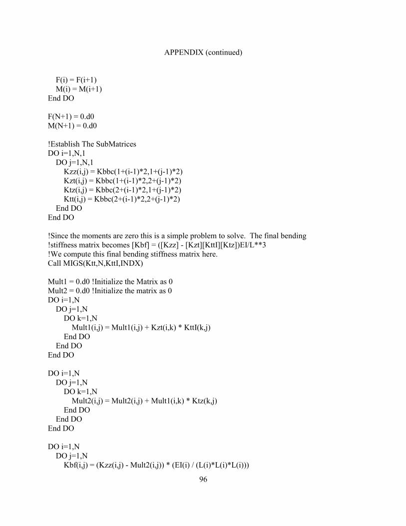
96


F(i) = F(i+1) M(i) = M(i+1) End DO F(N+1) = 0.d0 M(N+1) = 0.d0 !Establish The SubMatrices DO i=1,N,1 DO j=1,N,1 Kzz(i,j) = Kbbc(1+(i-1)*2,1+(j-1)*2) Kzt(i,j) = Kbbc(1+(i-1)*2,2+(j-1)*2) Ktz(i,j) = Kbbc(2+(i-1)*2,1+(j-1)*2) Ktt(i,j) = Kbbc(2+(i-1)*2,2+(j-1)*2) End DO End DO !Since the moments are zero this is a simple problem to solve. The final bending !stiffness matrix becomes [Kbf] = ([Kzz] - [Kzt][KttI][Ktz])EI/L**3 !We compute this final bending stiffness matrix here. Call MIGS(Ktt,N,KttI,INDX) Mult1 = 0.d0 !Initialize the Matrix as 0 Mult2 = 0.d0 !Initialize the matrix as 0 DO i=1,N DO j=1,N DO k=1,N Mult1(i,j) = Mult1(i,j) + Kzt(i,k) * KttI(k,j) End DO End DO End DO DO i=1,N DO j=1,N DO k=1,N Mult2(i,j) = Mult2(i,j) + Mult1(i,k) * Ktz(k,j) End DO End DO End DO DO i=1,N DO j=1,N Kbf(i,j) = (Kzz(i,j) - Mult2(i,j)) * (EI(i) / (L(i)*L(i)*L(i)))

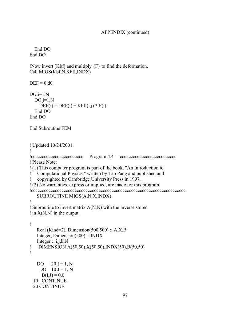
97


End DO End DO !Now invert [Kbf] and multiply {F} to find the deformation. Call MIGS(Kbf,N,KbfI,INDX) DEF = 0.d0 DO i=1,N DO j=1,N DEF(i) = DEF(i) + KbfI(i,j) * F(j) End DO End DO End Subroutine FEM ! Updated 10/24/2001. ! !cccccccccccccccccccccccc Program 4.4 cccccccccccccccccccccccccc ! Please Note: ! (1) This computer program is part of the book, "An Introduction to ! Computational Physics," written by Tao Pang and published and ! copyrighted by Cambridge University Press in 1997. ! (2) No warranties, express or implied, are made for this program. !ccccccccccccccccccccccccccccccccccccccccccccccccccccccccccccccccccccccc SUBROUTINE MIGS(A,N,X,INDX) ! ! Subroutine to invert matrix A(N,N) with the inverse stored ! in X(N,N) in the output. ! Real (Kind=2), Dimension(500,500) :: A,X,B Integer, Dimension(500) :: INDX Integer :: i,j,k,N ! DIMENSION A(50,50),X(50,50),INDX(50),B(50,50) ! DO 20 I = 1, N DO 10 J = 1, N B(I,J) = 0.0 10 CONTINUE 20 CONTINUE

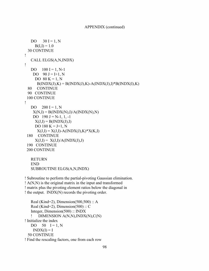
98


DO 30 I = 1, N B(I,I) = 1.0 30 CONTINUE ! CALL ELGS(A,N,INDX) ! DO 100 I = 1, N-1 DO 90 J = I+1, N DO 80 K = 1, N B(INDX(J),K) = B(INDX(J),K)-A(INDX(J),I)*B(INDX(I),K) 80 CONTINUE 90 CONTINUE 100 CONTINUE ! DO 200 I = 1, N X(N,I) = B(INDX(N),I)/A(INDX(N),N) DO 190 J = N-1, 1, -1 X(J,I) = B(INDX(J),I) DO 180 K = J+1, N X(J,I) = X(J,I)-A(INDX(J),K)*X(K,I) 180 CONTINUE X(J,I) = X(J,I)/A(INDX(J),J) 190 CONTINUE 200 CONTINUE RETURN END SUBROUTINE ELGS(A,N,INDX) ! Subroutine to perform the partial-pivoting Gaussian elimination. ! A(N,N) is the original matrix in the input and transformed ! matrix plus the pivoting element ratios below the diagonal in ! the output. INDX(N) records the pivoting order. Real (Kind=2), Dimension(500,500) :: A Real (Kind=2), Dimension(500) :: C Integer, Dimension(500) :: INDX ! DIMENSION A(N,N),INDX(N),C(N) ! Initialize the index DO 50 I = 1, N INDX(I) = I 50 CONTINUE ! Find the rescaling factors, one from each row

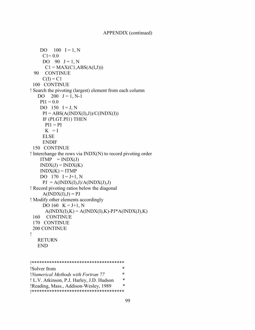
99


DO 100 I = 1, N C1= 0.0 DO 90 J = 1, N C1 = MAX(C1,ABS(A(I,J))) 90 CONTINUE C(I) = C1 100 CONTINUE ! Search the pivoting (largest) element from each column DO 200 J = 1, N-1 PI1 = 0.0 DO 150 I = J, N PI = ABS(A(INDX(I),J))/C(INDX(I)) IF (PI.GT.PI1) THEN PI1 = PI K = I ELSE ENDIF 150 CONTINUE ! Interchange the rows via INDX(N) to record pivoting order ITMP = INDX(J) INDX(J) = INDX(K) INDX(K) = ITMP DO 170 I = J+1, N PJ = A(INDX(I),J)/A(INDX(J),J) ! Record pivoting ratios below the diagonal A(INDX(I),J) = PJ ! Modify other elements accordingly DO 160 K = J+1, N A(INDX(I),K) = A(INDX(I),K)-PJ*A(INDX(J),K) 160 CONTINUE 170 CONTINUE 200 CONTINUE ! RETURN END !************************************* !Solver from * !Numerical Methods with Fortran 77 * ! L.V. Atkinson, P.J. Harley, J.D. Hudson * !Reading, Mass., Addison-Wesley, 1989 * !*************************************

100


SUBROUTINE GAUSSP (SIZE,N,A,B,STATUS,X,P) INTEGER :: I, J, K, N, PI, PK, PTINY, SIZE, SOLVED, STATUS REAL*8 :: MAX, MULT, PIVOT, TINY REAL*8 SUM PARAMETER (TINY=1E-10) PARAMETER(SOLVED=0,PTINY=1) INTEGER P(N) REAL*8 :: A(SIZE,SIZE), B(N), X(N) !Give P its initial values DO 10, I=1,N P(I)= I 10 END DO DO 20, I=1, N-1 ! Find the pivot MAX=0 PI = P(I) DO 30, J=I,N IF (ABS(A(P(J),I)) .GT. MAX) THEN MAX = ABS(A(P(J),I)) K = J END IF 30 END DO !Signal if pivot is too small IF (MAX.LE.TINY) THEN STATUS=PTINY GOTO 999 END IF !Otherwise swap elements in P if necessary IF (K.NE.I) THEN P(I) = P(K) P(K) = PI PI = P(I) END IF !Now do the elimination PIVOT = A(PI,I)

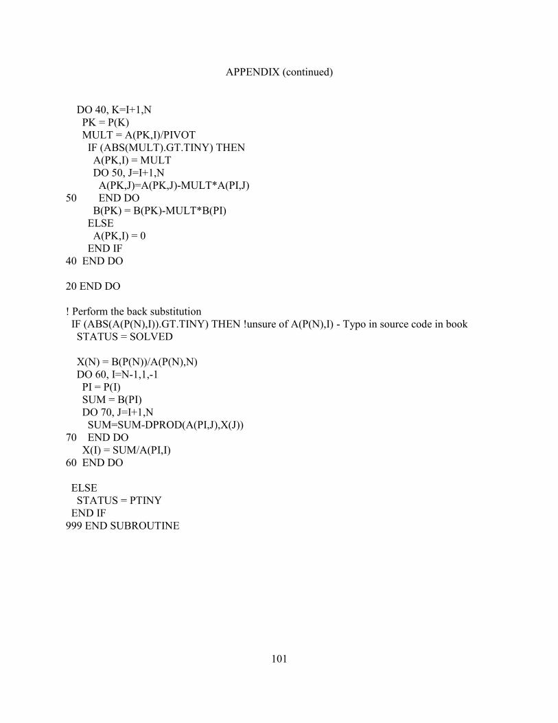
101


DO 40, K=I+1,N PK = P(K) MULT = A(PK,I)/PIVOT IF (ABS(MULT).GT.TINY) THEN A(PK,I) = MULT DO 50, J=I+1,N A(PK,J)=A(PK,J)-MULT*A(PI,J) 50 END DO B(PK) = B(PK)-MULT*B(PI) ELSE A(PK,I) = 0 END IF 40 END DO 20 END DO ! Perform the back substitution IF (ABS(A(P(N),I)).GT.TINY) THEN !unsure of A(P(N),I) - Typo in source code in book STATUS = SOLVED X(N) = B(P(N))/A(P(N),N) DO 60, I=N-1,1,-1 PI = P(I) SUM = B(PI) DO 70, J=I+1,N SUM=SUM-DPROD(A(PI,J),X(J)) 70 END DO X(I) = SUM/A(PI,I) 60 END DO ELSE STATUS = PTINY END IF 999 END SUBROUTINE

Documents

Non-planar lifting-line theory for fixed and deformable geometries