Embed Size (px)
Citation preview
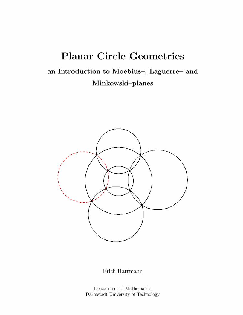
Planar Circle Geometries
an Introduction to Moebius–, Laguerre– and
Minkowski–planes
Erich Hartmann
Department of MathematicsDarmstadt University of Technology

2
Contents
0 INTRODUCTION 7
1 RESULTS ON AFFINE AND PROJECTIVE GEOMETRY 11
1.1 Affine planes . . . . . . . . . . . . . . . . . . . . . . . . . . . . . . . . . . 11
1.1.1 The axioms of an affine plane . . . . . . . . . . . . . . . . . . . . 11
1.1.2 Collineations of an affine plane . . . . . . . . . . . . . . . . . . . 12
1.1.3 Desarguesian affine planes . . . . . . . . . . . . . . . . . . . . . . 13
1.1.4 Pappian affine planes . . . . . . . . . . . . . . . . . . . . . . . . . 14
1.2 Projective planes . . . . . . . . . . . . . . . . . . . . . . . . . . . . . . . 15
1.2.1 The axioms of a projective plane . . . . . . . . . . . . . . . . . . 15
1.2.2 Collineations of a projective plane . . . . . . . . . . . . . . . . . . 15
1.2.3 Desarguesian projective planes . . . . . . . . . . . . . . . . . . . . 16
1.2.4 Homogeneous coordinates of a desarguesian plane . . . . . . . . . 17
1.2.5 Collineations of a desarguesian projective plane . . . . . . . . . . 17
1.2.6 Pappian projective planes . . . . . . . . . . . . . . . . . . . . . . 17
1.2.7 The groups PΓL(2, K), PGL(2, K) and PSL(2, K) . . . . . . . . 18
1.2.8 Basic 1–dimensional projective configurations . . . . . . . . . . . 19
2 OVALS AND CONICS 23
2.1 Oval, parabolic and hyperbolic curve . . . . . . . . . . . . . . . . . . . . 23
2.2 The ovals c1 and c2 . . . . . . . . . . . . . . . . . . . . . . . . . . . . . . 24
2.3 Properties of the ovals c1 and c2 . . . . . . . . . . . . . . . . . . . . . . 26
2.4 Oval conics and their properties . . . . . . . . . . . . . . . . . . . . . . 27
2.5 Oval conics in affine planes . . . . . . . . . . . . . . . . . . . . . . . . . 39
2.6 Finite ovals . . . . . . . . . . . . . . . . . . . . . . . . . . . . . . . . . . 40
2.7 Further examples of ovals . . . . . . . . . . . . . . . . . . . . . . . . . . 43
2.7.1 Translation–ovals . . . . . . . . . . . . . . . . . . . . . . . . . . . 43
2.7.2 Moufang–ovals . . . . . . . . . . . . . . . . . . . . . . . . . . . . 44
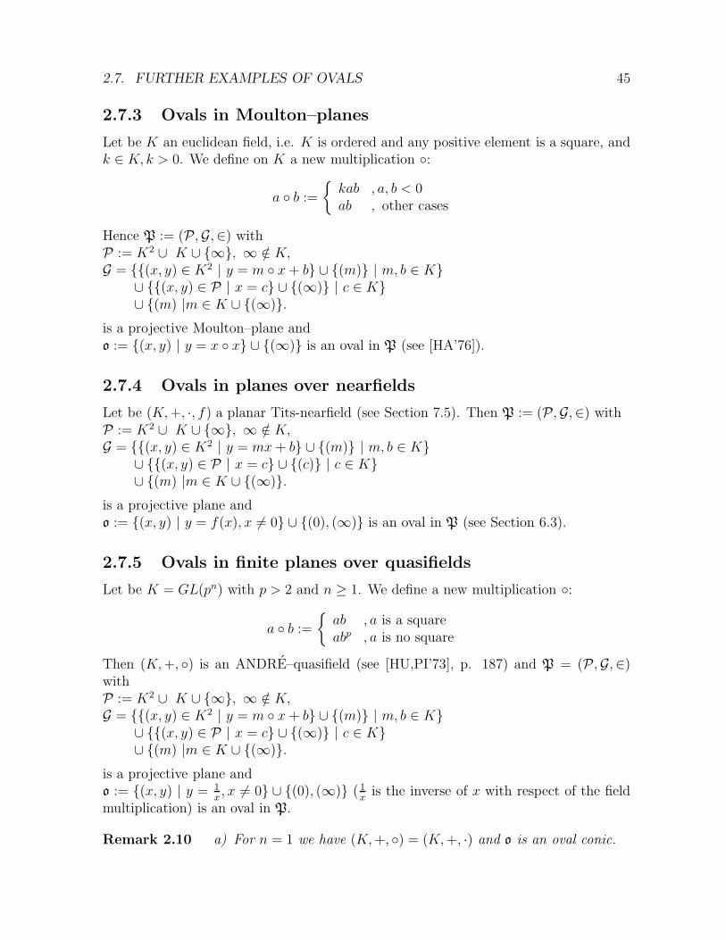
2.7.3 Ovals in Moulton–planes . . . . . . . . . . . . . . . . . . . . . . 45
2.7.4 Ovals in planes over nearfields . . . . . . . . . . . . . . . . . . . 45
2.7.5 Ovals in finite planes over quasifields . . . . . . . . . . . . . . . . 45
2.7.6 Real ovals on convex functions . . . . . . . . . . . . . . . . . . . . 46
3
3 MOEBIUS–PLANES 473.1 The classical real Moebius–plane . . . . . . . . . . . . . . . . . . . . . . 473.2 The axioms of a Moebius–plane . . . . . . . . . . . . . . . . . . . . . . . 483.3 Miquelian Moebius–planes . . . . . . . . . . . . . . . . . . . . . . . . . . 50
3.3.1 The incidence structure M(K, q) . . . . . . . . . . . . . . . . . . 503.3.2 Representation of M(K, q) over E . . . . . . . . . . . . . . . . . . 513.3.3 Automorphisms of M(K, q), M(K, q) is Moebius–plane . . . . . . 523.3.4 Cycle reflections . . . . . . . . . . . . . . . . . . . . . . . . . . . . 533.3.5 Angles in affine plane A(K, q) . . . . . . . . . . . . . . . . . . . . 553.3.6 Theorem of MIQUEL in M(K, q) . . . . . . . . . . . . . . . . . . 563.3.7 The sphere–model of a miquelian Moebius–plane . . . . . . . . . 593.3.8 Isomorphic miquelian Moebius–planes . . . . . . . . . . . . . . . . 60
3.4 Ovoidal Moebius–planes . . . . . . . . . . . . . . . . . . . . . . . . . . . 613.4.1 Plane model of an ovoidal Moebius–plane . . . . . . . . . . . . . . 633.4.2 Examples of ovoidal Moebius–planes . . . . . . . . . . . . . . . . 64
3.5 Non ovoidal Moebius–planes . . . . . . . . . . . . . . . . . . . . . . . . 643.6 Final remark . . . . . . . . . . . . . . . . . . . . . . . . . . . . . . . . . 65
4 LAGUERRE–PLANES 674.1 The classical real Laguerre–plane . . . . . . . . . . . . . . . . . . . . . . 674.2 The axioms of a Laguerre–plane . . . . . . . . . . . . . . . . . . . . . . . 684.3 Miquelian Laguerre–planes . . . . . . . . . . . . . . . . . . . . . . . . . . 70
4.3.1 The incidence structure L(K) . . . . . . . . . . . . . . . . . . . . 704.3.2 Automorphisms of L(K), L(K) is a Laguerre–plane . . . . . . . 704.3.3 Parabolic measure for angles in A(K) . . . . . . . . . . . . . . . 724.3.4 Theorem of MIQUEL in L(K) . . . . . . . . . . . . . . . . . . . . 72
4.4 Ovoidal Laguerre–planes . . . . . . . . . . . . . . . . . . . . . . . . . . . 744.4.1 Definition of an ovoidal Laguerre–plane . . . . . . . . . . . . . . . 744.4.2 The plane model of an ovoidal Laguerre–plane . . . . . . . . . . . 754.4.3 Examples of ovoidal Laguerre–planes . . . . . . . . . . . . . . . . 774.4.4 Automorphisms of an ovoidal Laguerre–plane L(K, f) . . . . . . . 774.4.5 The bundle theorem for Laguerre–planes . . . . . . . . . . . . . . 78
4.5 Non ovoidal Laguerre–planes . . . . . . . . . . . . . . . . . . . . . . . . . 794.6 Automorphisms of Laguerre–planes . . . . . . . . . . . . . . . . . . . . . 80
4.6.1 Transitivity properties of ovoidal Laguerre–planes . . . . . . . . . 83
5 MINKOWSKI–PLANES 875.1 The classical real Minkowski–plane . . . . . . . . . . . . . . . . . . . . . 875.2 The axioms of a Minkowski–plane . . . . . . . . . . . . . . . . . . . . . . 885.3 Miquelian Minkowski–planes . . . . . . . . . . . . . . . . . . . . . . . . 91
5.3.1 The incidence structure M(K) . . . . . . . . . . . . . . . . . . . . 915.3.2 Automorphisms of M(K). M(K) is a Minkowski–plane . . . . . 925.3.3 Hyperbolic measure for angles in M(K) . . . . . . . . . . . . . . 93
4
5
5.3.4 Theorem of MIQUEL in M(K) . . . . . . . . . . . . . . . . . . . 935.3.5 Cycle reflections and the Theorem of Miquel . . . . . . . . . . . 955.3.6 The hyperboloid model of a miquelian Minkowski–plane . . . . . 975.3.7 The bundle theorem for Minkowski–planes . . . . . . . . . . . . . 98
5.4 Minkowski–planes over TITS–nearfields . . . . . . . . . . . . . . . . . . 985.4.1 The incidence structure M(K, f) . . . . . . . . . . . . . . . . . . 985.4.2 Automorphisms of M(K, f). M(K, f) is a Minkowski–plane . . . 99
5.5 Minkowski–planes and sets of permutations . . . . . . . . . . . . . . . . 1005.5.1 Description of a Minkowski–plane by permutation sets . . . . . . 1005.5.2 Minkowski–planes over permutation groups . . . . . . . . . . . . 1015.5.3 Symmetry at a cycle. The rectangle axiom . . . . . . . . . . . . 1035.5.4 The symmetry axiom . . . . . . . . . . . . . . . . . . . . . . . . 1065.5.5 Minkowski–planes of even order . . . . . . . . . . . . . . . . . . . 110
5.6 Further Examples of Minkowski-planes . . . . . . . . . . . . . . . . . . . 1115.6.1 A method for the generation of finite Minkowski–planes . . . . . . 1115.6.2 Finite examples which do not fulfill (G) . . . . . . . . . . . . . . 1125.6.3 Real examples, which do not fulfill (G) . . . . . . . . . . . . . . . 113
5.7 Automorphisms of Minkowski–planes . . . . . . . . . . . . . . . . . . . . 114
6 Appendix: Quadrics 1176.1 Quadratic forms . . . . . . . . . . . . . . . . . . . . . . . . . . . . . . . 1176.2 Definition and properties of a quadric . . . . . . . . . . . . . . . . . . . . 1186.3 Quadratic sets . . . . . . . . . . . . . . . . . . . . . . . . . . . . . . . . 1216.4 Final remarks . . . . . . . . . . . . . . . . . . . . . . . . . . . . . . . . . 123
7 Appendix: Nearfields 1257.1 Definition of a nearfield and some rules . . . . . . . . . . . . . . . . . . 1257.2 Examples of nearfields . . . . . . . . . . . . . . . . . . . . . . . . . . . . 1267.3 Planar nearfields . . . . . . . . . . . . . . . . . . . . . . . . . . . . . . . 1267.4 Nearfields and sharply 2–transitive permutationgroups . . . . . . . . . . 1267.5 TITS–nearfields . . . . . . . . . . . . . . . . . . . . . . . . . . . . . . . . 127

6
Chapter 0
INTRODUCTION
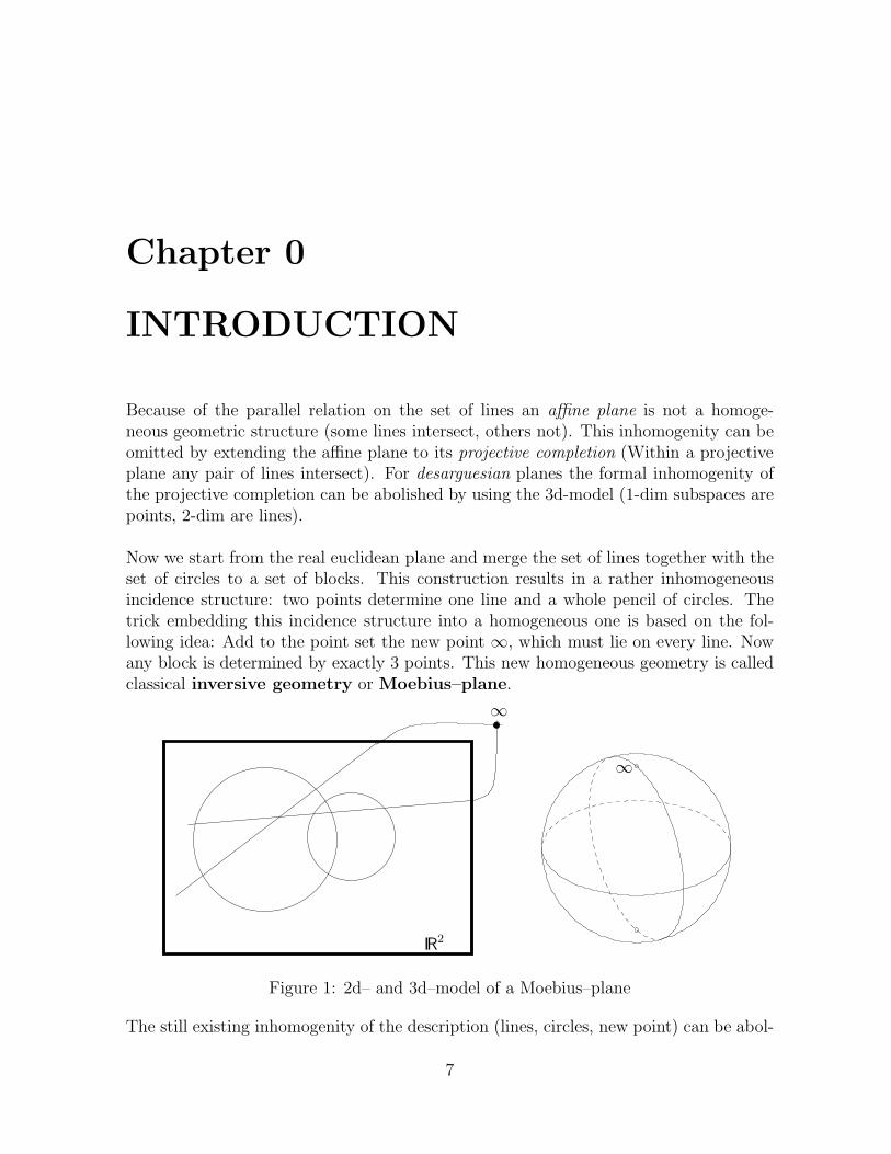
Because of the parallel relation on the set of lines an affine plane is not a homoge-neous geometric structure (some lines intersect, others not). This inhomogenity can beomitted by extending the affine plane to its projective completion (Within a projectiveplane any pair of lines intersect). For desarguesian planes the formal inhomogenity ofthe projective completion can be abolished by using the 3d-model (1-dim subspaces arepoints, 2-dim are lines).
Now we start from the real euclidean plane and merge the set of lines together with theset of circles to a set of blocks. This construction results in a rather inhomogeneousincidence structure: two points determine one line and a whole pencil of circles. Thetrick embedding this incidence structure into a homogeneous one is based on the fol-lowing idea: Add to the point set the new point ∞, which must lie on every line. Nowany block is determined by exactly 3 points. This new homogeneous geometry is calledclassical inversive geometry or Moebius–plane.
∞
∞
IR2
Figure 1: 2d– and 3d–model of a Moebius–plane
The still existing inhomogenity of the description (lines, circles, new point) can be abol-
7
8 CHAPTER 0. INTRODUCTION
ished by using a 3d-model. From a stereographic projection we learn: the classicalMoebius–plane is isomorphic to the geometry of plane sections (circles) on a sphere ineuclidean 3-space.
Analogously to the (axiomatic) projective plane one calls an incidence structure, whichexhibits essentially the same incidence properties, an (axiomatic) Moebius–plane (seeChapter 3). Expectedly there are a lot of Moebius–planes which are different from theclassical one.
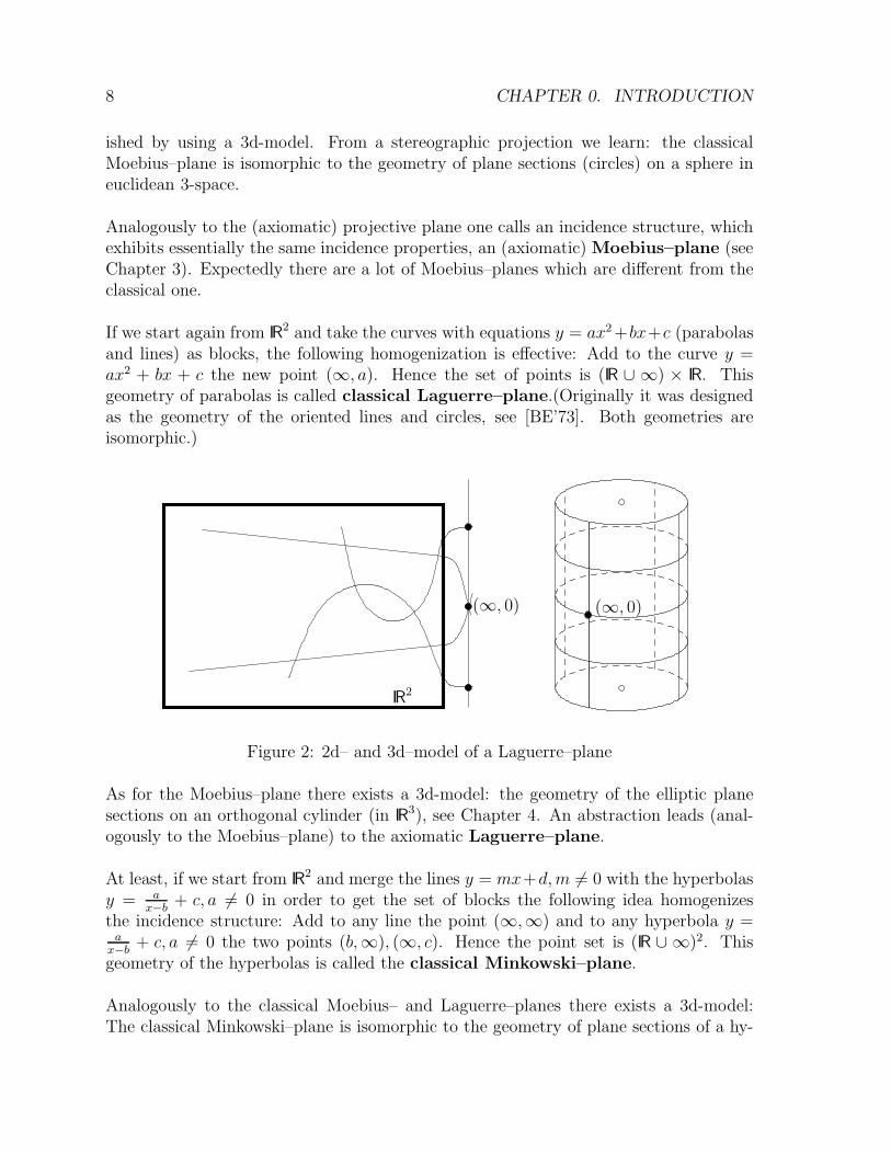
If we start again from IR2 and take the curves with equations y = ax2+bx+c (parabolas
and lines) as blocks, the following homogenization is effective: Add to the curve y =ax2 + bx + c the new point (∞, a). Hence the set of points is (IR ∪ ∞) × IR. Thisgeometry of parabolas is called classical Laguerre–plane.(Originally it was designedas the geometry of the oriented lines and circles, see [BE’73]. Both geometries areisomorphic.)
(∞, 0) (∞, 0)
IR2
Figure 2: 2d– and 3d–model of a Laguerre–plane
As for the Moebius–plane there exists a 3d-model: the geometry of the elliptic planesections on an orthogonal cylinder (in IR
3), see Chapter 4. An abstraction leads (anal-ogously to the Moebius–plane) to the axiomatic Laguerre–plane.
At least, if we start from IR2 and merge the lines y = mx+d,m 6= 0 with the hyperbolas
y = ax−b
+ c, a 6= 0 in order to get the set of blocks the following idea homogenizesthe incidence structure: Add to any line the point (∞,∞) and to any hyperbola y =a
x−b+ c, a 6= 0 the two points (b,∞), (∞, c). Hence the point set is (IR ∪ ∞)2. This
geometry of the hyperbolas is called the classical Minkowski–plane.
Analogously to the classical Moebius– and Laguerre–planes there exists a 3d-model:The classical Minkowski–plane is isomorphic to the geometry of plane sections of a hy-
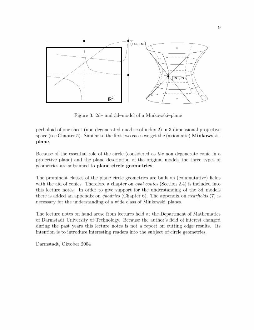
9
(∞,∞)
(∞,∞)
IR2
Figure 3: 2d– and 3d–model of a Minkowski–plane
perboloid of one sheet (non degenerated quadric of index 2) in 3-dimensional projectivespace (see Chapter 5). Similar to the first two cases we get the (axiomatic)Minkowski–plane.
Because of the essential role of the circle (considered as the non degenerate conic in aprojective plane) and the plane description of the original models the three types ofgeometries are subsumed to plane circle geometries.
The prominent classes of the plane circle geometries are built on (commutative) fieldswith the aid of conics. Therefore a chapter on oval conics (Section 2.4) is included intothis lecture notes. In order to give support for the understanding of the 3d–modelsthere is added an appendix on quadrics (Chapter 6). The appendix on nearfields (7) isnecessary for the understanding of a wide class of Minkowski–planes.
The lecture notes on hand arose from lectures held at the Department of Mathematicsof Darmstadt University of Technology. Because the author’s field of interest changedduring the past years this lecture notes is not a report on cutting edge results. Itsintention is to introduce interesting readers into the subject of circle geometries.
Darmstadt, Oktober 2004
10 CHAPTER 0. INTRODUCTION
Chapter 1
RESULTS ON AFFINE ANDPROJECTIVE GEOMETRY
Literature: [BR’76], [DE’68], [DE,PR’76], [HU,PI’73], [LE’65], [LI’78], [PI’55]
1.1 Affine planes
1.1.1 The axioms of an affine plane
Let be P 6= ∅ a set, the set of points, and G 6= ∅ a subset of the power set of P, theset of lines. A point is called incident with a line g, if P ∈ g. Two lines g, h are calledparallel (designation: g ‖ h) if g = h or g ∩ h = ∅.
The incidence structure A := (P,G,∈) is called affine plane if the following axiomshold:
A1: For any pair of points P,Q there exists one and only one line g with P,Q ∈ g.
A2: For any line g and any point P there exists one and only one line g′ with P ∈ g′
and g ‖ g′.
A3: There are three points not on a common line.
Three points P,Q,R are called collinear if there is a line g with P,Q,R ∈ g.
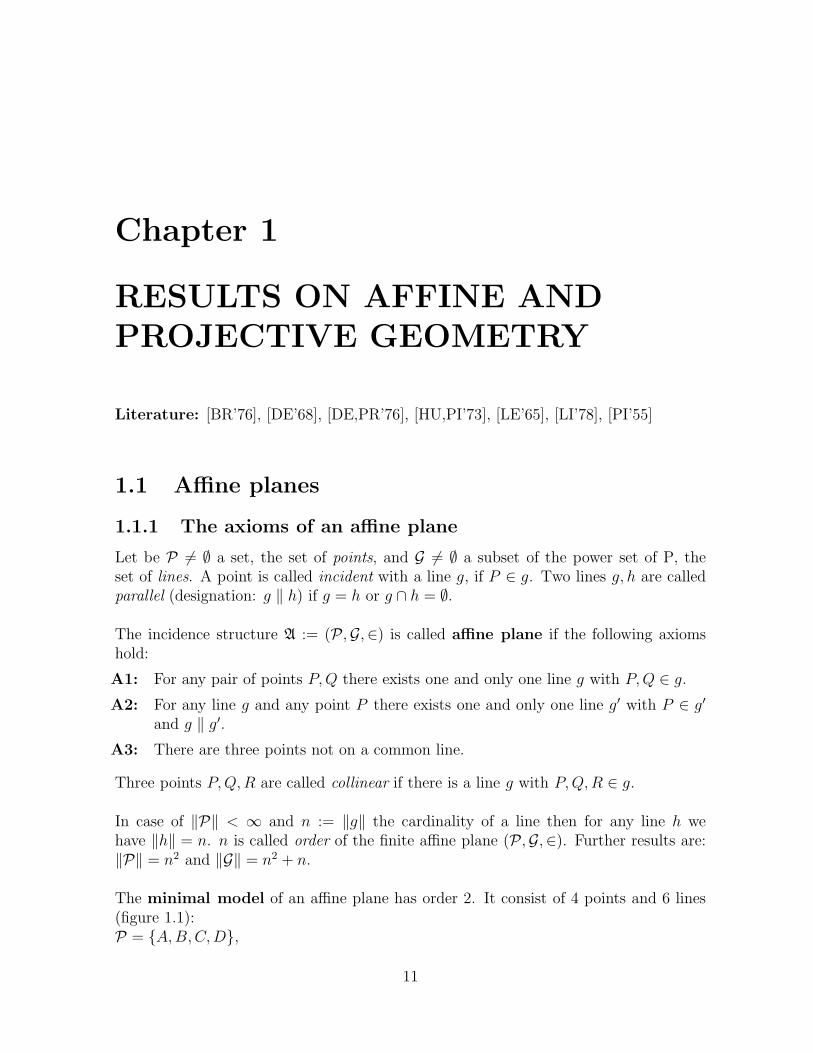
In case of ‖P‖ < ∞ and n := ‖g‖ the cardinality of a line then for any line h wehave ‖h‖ = n. n is called order of the finite affine plane (P,G,∈). Further results are:‖P‖ = n2 and ‖G‖ = n2 + n.
The minimal model of an affine plane has order 2. It consist of 4 points and 6 lines(figure 1.1):P = {A,B,C,D},
11
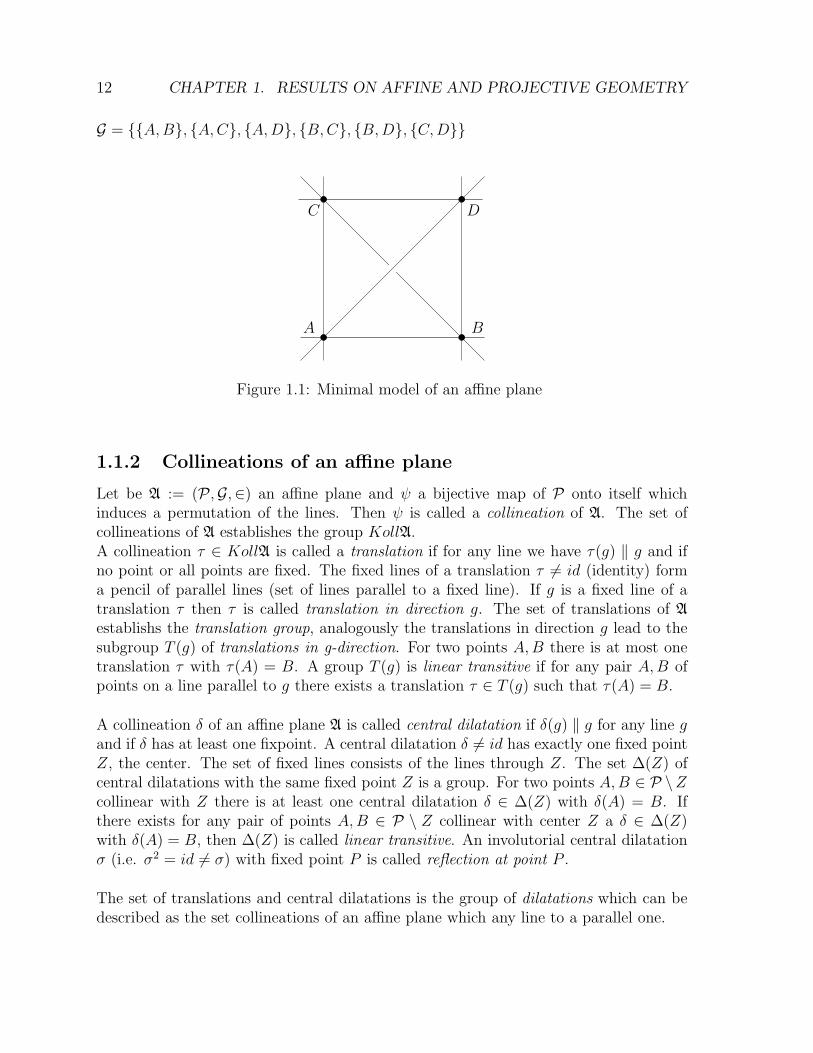
12 CHAPTER 1. RESULTS ON AFFINE AND PROJECTIVE GEOMETRY
G = {{A,B}, {A,C}, {A,D}, {B,C}, {B,D}, {C,D}}
A B
C D
Figure 1.1: Minimal model of an affine plane
1.1.2 Collineations of an affine plane
Let be A := (P,G,∈) an affine plane and ψ a bijective map of P onto itself whichinduces a permutation of the lines. Then ψ is called a collineation of A. The set ofcollineations of A establishes the group KollA.A collineation τ ∈ KollA is called a translation if for any line we have τ(g) ‖ g and ifno point or all points are fixed. The fixed lines of a translation τ 6= id (identity) forma pencil of parallel lines (set of lines parallel to a fixed line). If g is a fixed line of atranslation τ then τ is called translation in direction g. The set of translations of Aestablishs the translation group, analogously the translations in direction g lead to thesubgroup T (g) of translations in g-direction. For two points A,B there is at most onetranslation τ with τ(A) = B. A group T (g) is linear transitive if for any pair A,B ofpoints on a line parallel to g there exists a translation τ ∈ T (g) such that τ(A) = B.
A collineation δ of an affine plane A is called central dilatation if δ(g) ‖ g for any line gand if δ has at least one fixpoint. A central dilatation δ 6= id has exactly one fixed pointZ, the center. The set of fixed lines consists of the lines through Z. The set ∆(Z) ofcentral dilatations with the same fixed point Z is a group. For two points A,B ∈ P \Zcollinear with Z there is at least one central dilatation δ ∈ ∆(Z) with δ(A) = B. Ifthere exists for any pair of points A,B ∈ P \ Z collinear with center Z a δ ∈ ∆(Z)with δ(A) = B, then ∆(Z) is called linear transitive. An involutorial central dilatationσ (i.e. σ2 = id 6= σ) with fixed point P is called reflection at point P .
The set of translations and central dilatations is the group of dilatations which can bedescribed as the set collineations of an affine plane which any line to a parallel one.
1.1. AFFINE PLANES 13
A collineation α of an affine plane A is called axial affinity, if the set of fixed points ofα comprises the points of a line a. The fixed lines of α are line a and a pencil of parallellines Πα. Affinity α is a shear at line a, if a ∈ Πα and an axial dilatation at a, if a /∈ Πα.If for a line z we have z ∈ Πα collineation α is called axial affinity in z-direction. Theset A(a) of axial affinities with axis a is a group, alike the subset A(a, z) of A(a) withdirection z. Group A(a, z) is called linear transitive if for any pair P,Q ∈ P \ a whoseconnection line is parallel to z there exists an α ∈ A(a, z) with α(P ) = Q.An axial affinity is uniquely determined by a pair of point and image point not on theaxis.
1.1.3 Desarguesian affine planes
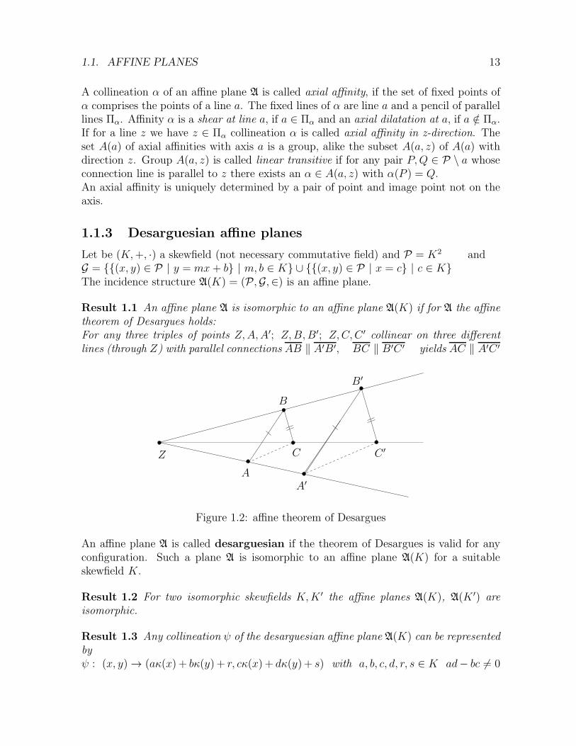
Let be (K,+, ·) a skewfield (not necessary commutative field) and P = K2 andG = {{(x, y) ∈ P | y = mx+ b} | m, b ∈ K} ∪ {{(x, y) ∈ P | x = c} | c ∈ K}The incidence structure A(K) = (P,G,∈) is an affine plane.
Result 1.1 An affine plane A is isomorphic to an affine plane A(K) if for A the affinetheorem of Desargues holds:For any three triples of points Z,A,A′; Z,B,B′; Z,C, C ′ collinear on three differentlines (through Z) with parallel connections AB ‖ A′B′, BC ‖ B′C ′ yields AC ‖ A′C ′
Z
A
B
C
A′
B′
C ′
Figure 1.2: affine theorem of Desargues
An affine plane A is called desarguesian if the theorem of Desargues is valid for anyconfiguration. Such a plane A is isomorphic to an affine plane A(K) for a suitableskewfield K.
Result 1.2 For two isomorphic skewfields K,K ′ the affine planes A(K), A(K ′) areisomorphic.
Result 1.3 Any collineation ψ of the desarguesian affine plane A(K) can be representedbyψ : (x, y) → (aκ(x) + bκ(y) + r, cκ(x) + dκ(y) + s) with a, b, c, d, r, s ∈ K ad− bc 6= 0
14 CHAPTER 1. RESULTS ON AFFINE AND PROJECTIVE GEOMETRY
and an isomorphism κ of skewfield K.If κ = id then ψ is called affinity.Especially we get:
a) κ = id, a = d = 1, b = c = 0 the translation (x, y) → (x+ r, y + s),
b) κ = id, a 6= 0, b = c = r = s = 0, d = 1 the axial affinity at the y-axis (x, y) →(ax, y),
c) κ = id, a = 1, b = r = s = 0, d = 1 the shear at the y-axis (x, y) → (x, y + cx),
d) κ(x) = t−1xt, a = t, b = c = r = s = 0, d = t the central dilatation at point (0, 0)(x, y) → (xt, yt),
Result 1.4 a) An affine plane A is desarguesian if and only if any central dilatationgroup ∆(P ), P ∈ P, is linear transitive.b) An affine plane A is desarguesian if and only if any group A(a, z), a, z ∈ G, of axialaffinities is linear transitive.
Result 1.5 The group of affinities operates transitively on the set of triangles (triplesof non collinear points).
Result 1.6 The skewfield K of coordinates of a desarguesian affine plane A(K) is ofcharacteristic 2 (i.e. 1+1 = 0) if there is one parallelogram with parallel diagonal lines.
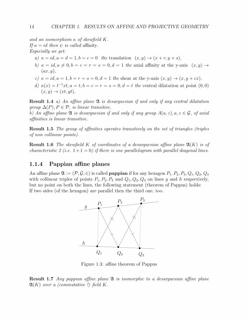
1.1.4 Pappian affine planes
An affine plane A := (P,G,∈) is called pappian if for any hexagon P1, P2, P3, Q1, Q2, Q3
with collinear triples of points P1, P2, P3 and Q1, Q2, Q3 on lines g and h respectively,but no point on both the lines, the following statement (theorem of Pappus) holds:If two sides (of the hexagon) are parallel then the third one, too.
g
h
P1P2
P3
Q1 Q2 Q3
Figure 1.3: affine theorem of Pappus
Result 1.7 Any pappian affine plane A is isomorphic to a desarguesian affine planeA(K) over a (commutative !) field K.
1.2. PROJECTIVE PLANES 15
Remark: For a pappian affine plane the group of affinities comprises the set of centraldilatations.
1.2 Projective planes
1.2.1 The axioms of a projective plane
Let be P 6= ∅ a set, the set of points, and G 6= ∅ a subset of the power set of P, the setof lines. A point P is called incident with a line g, if P ∈ g.The incidence structure P := (P,G,∈) is called projective plane if the followingaxioms hold:
P1: For any pair of points P,Q there exists one and only one line g with P,Q ∈ g.
P2: For any pair of lines g, h there exists one and only one point P with g ∩ h = {P}.
P3: There are four points, no three collinear (quadrilateral).
Three points P,Q,R are collinear if there is a line with P,Q,R ∈ g.
For |P| < ∞ and n := |g| − 1 we have |h| = n + 1 for any line h ∈ G. The integer n iscalled order of the finite projective plane (P,G,∈).From combinatorics we get: |PC| = |G| = n2 + n+ 1.
Result 1.8 a) Let be A = (P,G,∈) an affine plane and U the set of classes of parallellines on G, then the incidence structure A := (P ′,G ′,∈) withP ′ := P ∪ U and G ′ := {g ∪ ug | g ∈ P, ug ∈ U with g ∈ ug} ∪ {U}is a projective plane.A is the projective completion of A.
b) Let be P = (P,G,∈) a projective plane and g∞ ∈ G. Then the incidence structureP := (P ′,G ′,∈) with P ′ := P \ g∞ and G ′ := {g \ g∞ | g ∈ G \ {g∞}}is an affine plane.
1.2.2 Collineations of a projective plane
Let be (P,G,∈) a projective plane and ψ a permutation of its point set P which inducesa permutation of the lines. ψ is called a collineation of P. A collineation π that fixes thepoints of a line g and any line through a fixed point P (pencil of lines) is called a centralcollineation or perspectivity with axis g and center P , short: (g, P ) − perspectivity.In case of P ∈ g π is called elation otherwise (P /∈ g) homology. The set of centralcollineations with same axis g and center P form group Π(g, P ). The group Π(g, p) islinear transitive if for any pair of points A,B ∈ P \ (g ∪ {P}) collinear with center Pthere exists a π ∈ Π(g, P ) such that π(A) = B (For short: A is (g, P ) − transitive).The group Π generated by the central collineations is the group of projectivities.
16 CHAPTER 1. RESULTS ON AFFINE AND PROJECTIVE GEOMETRY
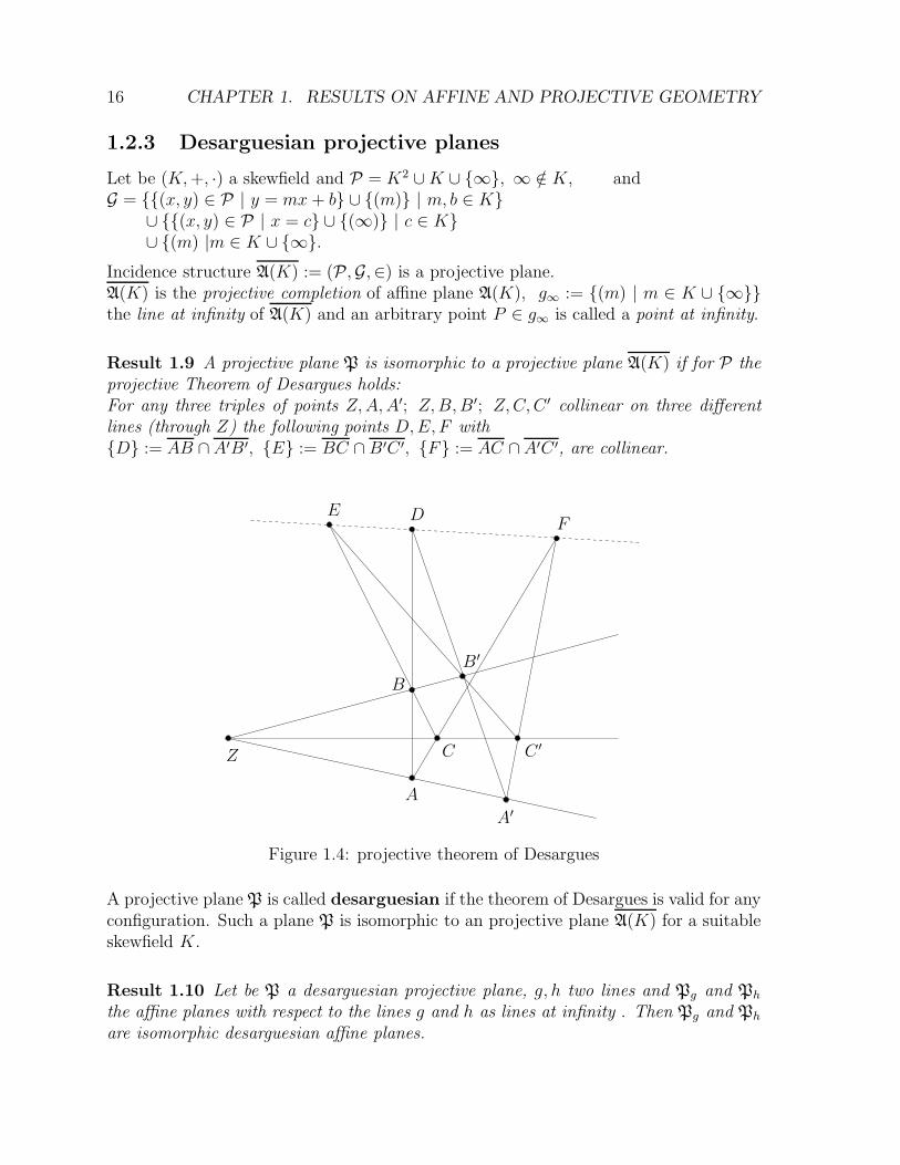
1.2.3 Desarguesian projective planes
Let be (K,+, ·) a skewfield and P = K2 ∪K ∪ {∞}, ∞ /∈ K, andG = {{(x, y) ∈ P | y = mx+ b} ∪ {(m)} | m, b ∈ K}
∪ {{(x, y) ∈ P | x = c} ∪ {(∞)} | c ∈ K}∪ {(m) |m ∈ K ∪ {∞}.
Incidence structure A(K) := (P,G,∈) is a projective plane.A(K) is the projective completion of affine plane A(K), g∞ := {(m) | m ∈ K ∪ {∞}}the line at infinity of A(K) and an arbitrary point P ∈ g∞ is called a point at infinity.
Result 1.9 A projective plane P is isomorphic to a projective plane A(K) if for P theprojective Theorem of Desargues holds:For any three triples of points Z,A,A′; Z,B,B′; Z,C, C ′ collinear on three differentlines (through Z) the following points D,E, F with{D} := AB ∩A′B′, {E} := BC ∩ B′C ′, {F} := AC ∩A′C ′, are collinear.
Z
A
B
C
DEF
A′
B′
C ′
Figure 1.4: projective theorem of Desargues
A projective plane P is called desarguesian if the theorem of Desargues is valid for anyconfiguration. Such a plane P is isomorphic to an projective plane A(K) for a suitableskewfield K.
Result 1.10 Let be P a desarguesian projective plane, g, h two lines and Pg and Ph
the affine planes with respect to the lines g and h as lines at infinity . Then Pg and Ph
are isomorphic desarguesian affine planes.
1.2. PROJECTIVE PLANES 17
1.2.4 Homogeneous coordinates of a desarguesian plane
Let be (K,+, ·) a skewfield, K3 the 3-dimensional right vector space on K and< (x1, x2, x3) > the 1-dimensional subspace determined by 0 6= (x1, x2, x3) ∈ K3. ForP := {< (x1, x2, x3) > | 0 6= (x1, x2, x3) ∈ K3} andG := {{< (x1, x2, x3) >∈ P | ax1 + bx2 + cx3 = 0} | 0 6= (a, b, c) ∈ K3}
the incidence structure P(K) := (P,G,∈) is a projective plane.
Result 1.11 P(K) is isomorphic to the desarguesian projective plane A(K).
P(K) is a representation of A(K) in homogeneous coordinates.If one chooses the isomorphism mentioned in the result above in such a way that theline at infinity of A(K) has the equation x3 = 0 then we get the following spatial rep-resentation (P ′,G ′,∈) of the affine plane A(K):
P ′ := {< (x, y, 1) > | x, y ∈ K}G ′ := {{< (x, y, 1) > | ax+ by + c = 0} | 0 6= (a, b) ∈ K2, c ∈ K}
1.2.5 Collineations of a desarguesian projective plane
Let be (K,+, ·) a skewfield, V a right vector space over K and ψ a bijection from V
onto itself withψ(xk + yl) = ψ(x)κ(k) + ψ(y)κ(l) where κ is an automorphism of the skewfield K.Then ψ is called a semi linear map of V. The set of semi linear maps of V is the groupΓL(V, K). The linear maps (i.e. κ = id) are a subgroup GL(V, K) of ΓL(V, K).In case of finite dimension n ≥ 1 of V one uses the following assignments:ΓL(n,K) := ΓL(V, K) and GL(n,K) := GL(V, K).For example: ψ ∈ ΓL(2, K) has the following representation:(x1, x2) → (aκ(x1) + bκ(x2), cκ(x1) + dκ(x2) with ad− bc 6= 0.
Any semi linear map ψ of vector space K3 induces a collineation of the desarguesianprojective plane P(K). Group ΓL(3, K) induces the collineation group PΓL(3, K) andGl(3, K) induces PGL(3, K).
Result 1.12 a) PΓL(3, K) is the set of all collineations of P(K).b) PGL(3, K) is the set of all projectivities of P(K).
Result 1.13 For a desarguesian projective plane PGL(3, K) operates transitive on theset of quadrangles in “general position” (i.e. no three points are collinear).
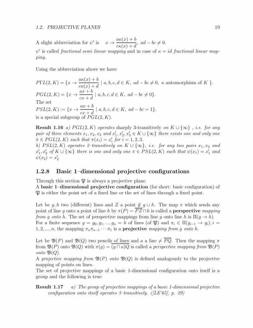
1.2.6 Pappian projective planes
A projective plane P = (P,G,∈) is called pappian ifP fulfills the (projective) Theoremof Pappus :
18 CHAPTER 1. RESULTS ON AFFINE AND PROJECTIVE GEOMETRY
Let be P1, P2, P3, Q1, Q2, Q3 a hexagon with collinear triples of points P1, P2, P3 andQ1, Q2, Q3 on two lines g and h respectively, but no point on both the lines. Then thefollowing three pointsA := P1Q2 ∩ P2Q1, B := P1Q3 ∩ P3Q1, C := P2Q3 ∩ P3Q2 are collinear.
g
h
P1P2
P3
Q1 Q2 Q3
A B C
Figure 1.5: projective Theorem of Pappus
Result 1.14 Any pappian projective plane P is isomorphic to a desarguesian projectiveplane P(K) over a (commutative !) field K.
Result 1.15 (PICKERT, see [KA’73])A projective plane is pappian if and only if the theorem of Pappus is fulfilled for hexagonson two fixed lines g, h.
1.2.7 The groups PΓL(2, K), PGL(2, K) and PSL(2, K)
Let be (K,+, ·) a field andP1(K) := {< (x1, x2) > | 0 6= (x1, x2) ∈ K2} and A1(K) := K ∪ {∞}the homogeneous and inhomogeneous representation of the projective line on K, respec-tively.Because of their definition PΓL(2, K) and PGL(2, K) are groups of permutations ofP1(K). For any ψ ∈ PΓL(2, K) there exist a, b, c, d ∈ K and an automorphism κ offield K such thatψ : < (x1, x2) >→< (aκ(x1) + bκ(x2), cκ(x1) + dκ(x2)) > with ad− bc 6= 0.
With the bijection< (1, 0) >→ ∞, < (x, 1) >→ x from P1(K) onto K ∪ {∞} we recognize that ψinduces on K ∪ {∞} the permutation ψ′ with the following effect:
∞ →
{ a
c, if c 6= 0
∞ , if c = 0, x→
aκ(x) + b
cκ(x) + d, if cκ(x) + d 6= 0
∞ , if cκ(x) + d = 0for x ∈ K.
1.2. PROJECTIVE PLANES 19
A slight abbreviation for ψ′ is x→aκ(x) + b
cκ(x) + d, ad− bc 6= 0.
ψ′ is called fractional semi linear mapping and in case of κ = id fractional linear map-ping.
Using the abbreviation above we have:
PΓL(2, K) = {x→aκ(x) + b
cκ(x) + d| a, b, c, d ∈ K, ad− bc 6= 0, κ automorphism of K }.
PGL(2, K) = {x→ax+ b
cx+ d| a, b, c, d ∈ K, ad− bc 6= 0}.
The set
PSL(2, K) := {x→ax+ b
cx+ d| a, b, c, d ∈ K, ad− bc = 1}.
is a special subgroup of PGL(2, K).
Result 1.16 a) PGL(2, K) operates sharply 3-transitively on K ∪ {∞} , i.e. for anypair of three elements x1, x2, x3 and x′1, x
′2, x
′3 ∈ K ∪ {∞} there exists one and only one
π ∈ PGL(2, K) such that π(xi) = x′i for i = 1, 2, 3.b) PSL(2, K) operates 2–transitively on K ∪ {∞}, i.e. for any two pairs x1, x2 andx′1, x
′2 of K ∪ {∞} there is one and only one π ∈ PSL(2, K) such that ψ(x1) = x′1 and
ψ(x2) = x′2
1.2.8 Basic 1–dimensional projective configurations
Through this section P is always a projective plane.A basic 1–dimensional projective configuration (for short: basic configuration) ofP is either the point set of a fixed line or the set of lines through a fixed point.
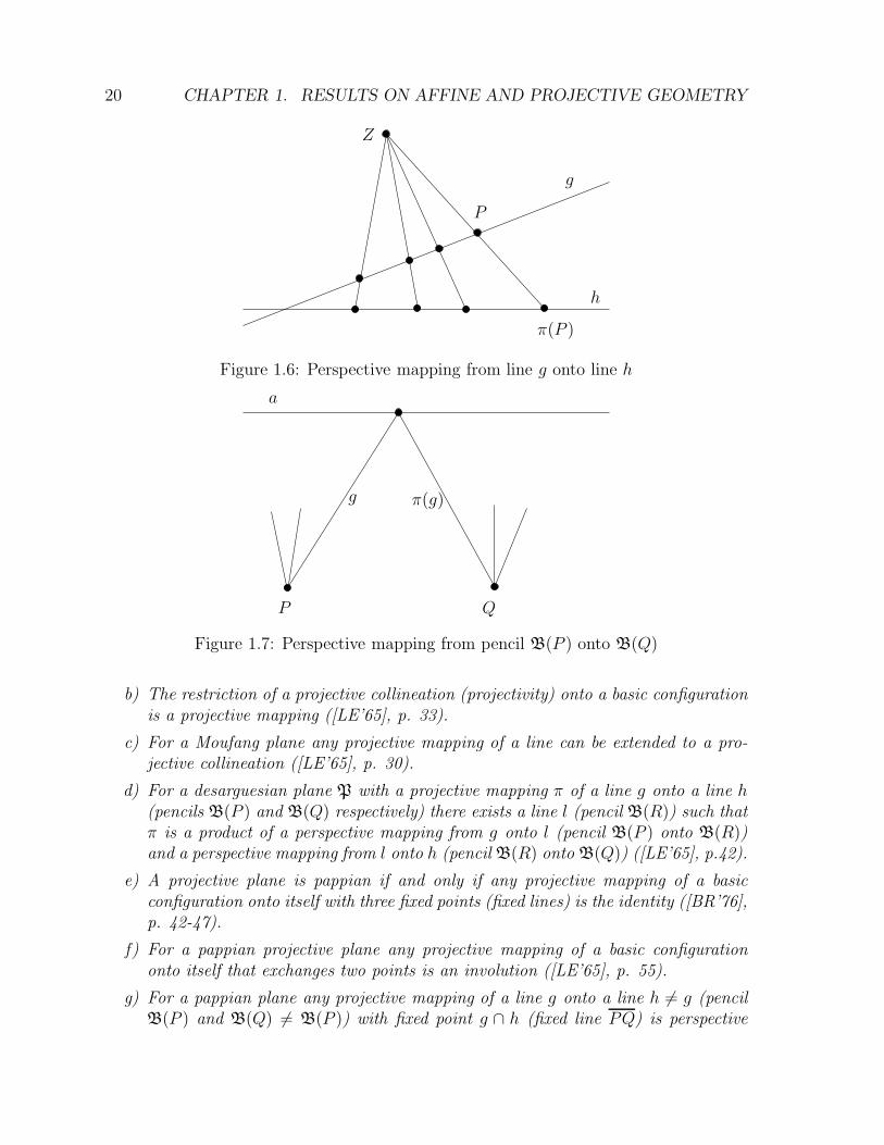
Let be g, h two (different) lines and Z a point /∈ g ∪ h. The map π which sends anypoint of line g onto a point of line h by π(P ) = PZ∩h is called a perspective mappingfrom g onto h. The set of perspective mappings from line g onto line h is Π(g → h).For a finite sequence g = g0, g1, ..., gn = h of lines (of P) and πi ∈ Π(gi−1 → gi), i =1, 2, ..., n, the mapping πnπn−1 · · ·π1 is a projective mapping from g onto h.
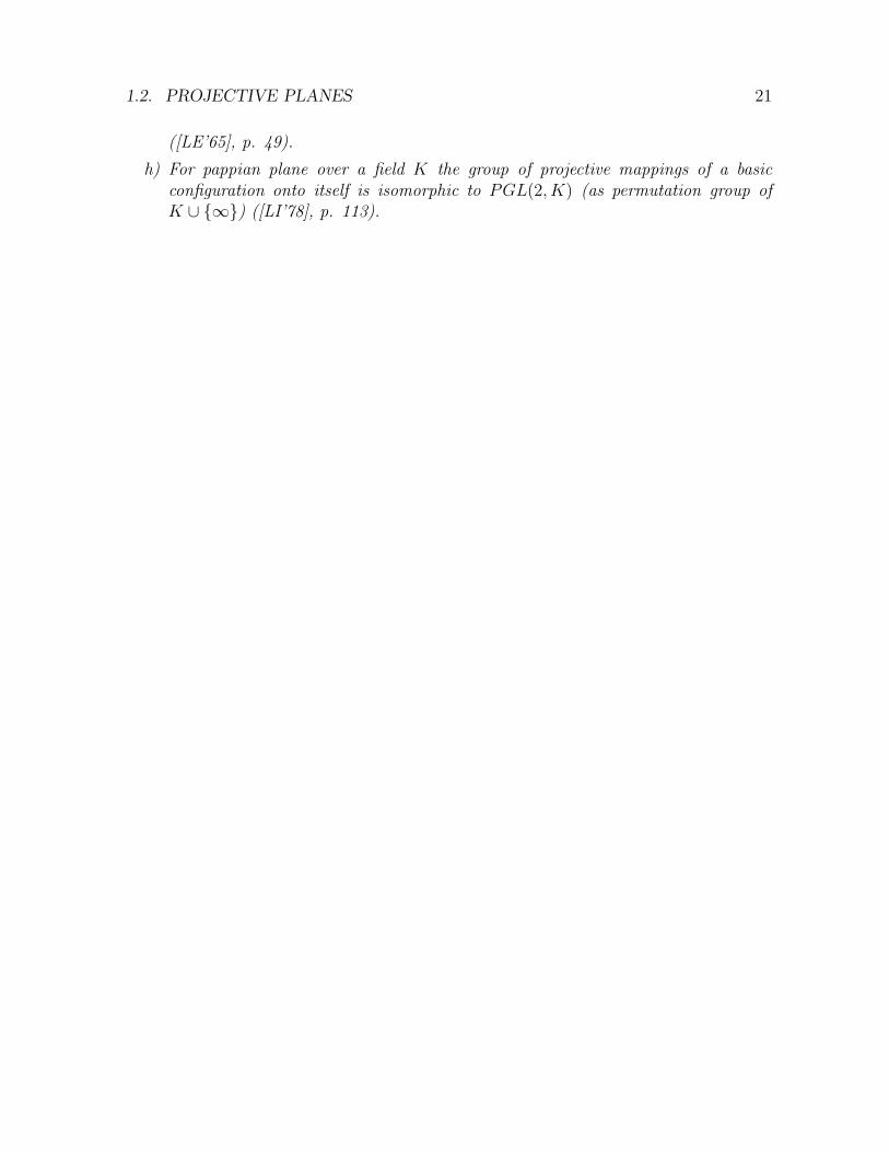
Let be B(P ) and B(Q) two pencils of lines and a a line 6= PQ. Then the mapping πfrom B(P ) onto B(Q) with π(g) = (g ∩ a)Q is called a perspective mapping from B(P )onto B(Q).A projective mapping from B(P ) onto B(Q) is defined analogously to the projectivemapping of points on lines.The set of projective mappings of a basic 1-dimensional configuration onto itself is agroup and the following is true:
Result 1.17 a) The group of projective mappings of a basic 1-dimensional projectiveconfiguration onto itself operates 3–transitively. ([LE’65], p. 29)
20 CHAPTER 1. RESULTS ON AFFINE AND PROJECTIVE GEOMETRY
Z
P
π(P )
g
h
Figure 1.6: Perspective mapping from line g onto line h
a
P Q
π(g)g
Figure 1.7: Perspective mapping from pencil B(P ) onto B(Q)
b) The restriction of a projective collineation (projectivity) onto a basic configurationis a projective mapping ([LE’65], p. 33).
c) For a Moufang plane any projective mapping of a line can be extended to a pro-jective collineation ([LE’65], p. 30).
d) For a desarguesian plane P with a projective mapping π of a line g onto a line h(pencils B(P ) and B(Q) respectively) there exists a line l (pencil B(R)) such thatπ is a product of a perspective mapping from g onto l (pencil B(P ) onto B(R))and a perspective mapping from l onto h (pencil B(R) onto B(Q)) ([LE’65], p.42).
e) A projective plane is pappian if and only if any projective mapping of a basicconfiguration onto itself with three fixed points (fixed lines) is the identity ([BR’76],p. 42-47).
f) For a pappian projective plane any projective mapping of a basic configurationonto itself that exchanges two points is an involution ([LE’65], p. 55).
g) For a pappian plane any projective mapping of a line g onto a line h 6= g (pencilB(P ) and B(Q) 6= B(P )) with fixed point g ∩ h (fixed line PQ) is perspective
1.2. PROJECTIVE PLANES 21
([LE’65], p. 49).
h) For pappian plane over a field K the group of projective mappings of a basicconfiguration onto itself is isomorphic to PGL(2, K) (as permutation group ofK ∪ {∞}) ([LI’78], p. 113).
22 CHAPTER 1. RESULTS ON AFFINE AND PROJECTIVE GEOMETRY
Chapter 2
OVALS AND CONICS
Literature: [BR’76], [DE’68], [HU,PI’73], [LE’65], [LI’78], [PI’55]
2.1 Oval, parabolic and hyperbolic curve
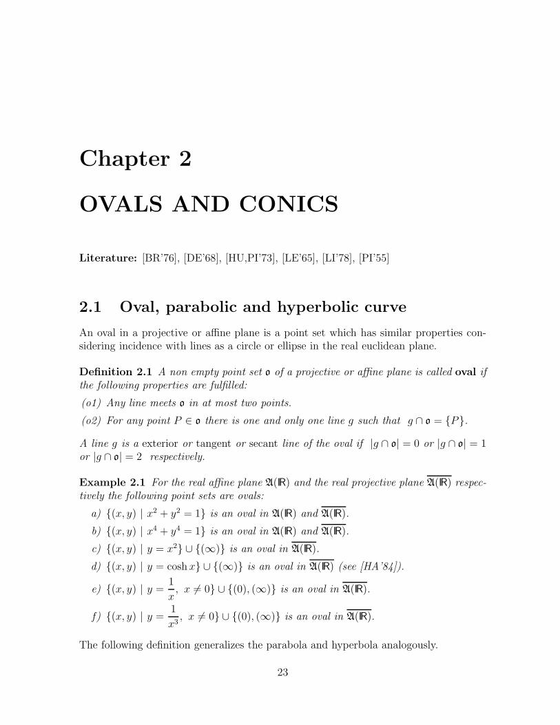
An oval in a projective or affine plane is a point set which has similar properties con-sidering incidence with lines as a circle or ellipse in the real euclidean plane.
Definition 2.1 A non empty point set o of a projective or affine plane is called oval ifthe following properties are fulfilled:
(o1) Any line meets o in at most two points.
(o2) For any point P ∈ o there is one and only one line g such that g ∩ o = {P}.
A line g is a exterior or tangent or secant line of the oval if |g ∩ o| = 0 or |g ∩ o| = 1or |g ∩ o| = 2 respectively.
Example 2.1 For the real affine plane A(IR) and the real projective plane A(IR) respec-tively the following point sets are ovals:
a) {(x, y) | x2 + y2 = 1} is an oval in A(IR) and A(IR).
b) {(x, y) | x4 + y4 = 1} is an oval in A(IR) and A(IR).
c) {(x, y) | y = x2} ∪ {(∞)} is an oval in A(IR).
d) {(x, y) | y = cosh x} ∪ {(∞)} is an oval in A(IR) (see [HA’84]).
e) {(x, y) | y =1
x, x 6= 0} ∪ {(0), (∞)} is an oval in A(IR).
f) {(x, y) | y =1
x3, x 6= 0} ∪ {(0), (∞)} is an oval in A(IR).
The following definition generalizes the parabola and hyperbola analogously.
23
24 CHAPTER 2. OVALS AND CONICS
Definition 2.2 Let A be an affine plane, A its projective completion and g∞ the lineat infinity.
a) A point set p of A is a parabolic curve if there is a point U ∈ g∞ such thato := p ∪ {U} is an oval in A. U is the point at infinity of p.
b) A point set h of A is a hyperbolic curve if there are two points U, V ∈ g∞ suchthat o := p ∪ {U, V } is an oval in A. U, V are the points at infinity of h.
Example 2.2 For the real affine plane A(IR) the following statements are true:
a) {(x, y) | y = x2} is a parabolic curve in A(IR) with U = (∞).
b) {(x, y) | y = cosh x} is a parabolic curve in A(IR) with U = (∞).
c) {(x, y) | y =1
x, x 6= 0} is a hyperbolic curve in A(IR) with U = (∞), V = (0).
d) {(x, y) | x2−y2 = 1, x 6= 0} is a hyperbolic curve in A(IR) with U = (1), V = (−1).
Remark 2.1 The point at infinity of a parabolic curve is not in any case uniquelydetermined !
Apparently the following statement holds:
Lemma 2.1 a) Let be A an affine plane, ϕ a collineation, o an oval, p a paraboliccurve and h a hyperbolic curve. Then ϕ(o) is an oval , ϕ(p) a parabolic curve andϕ(h) a hyperbolic curve, too.
b) Let be P a projective plane, ϕ a collineation and o an oval. Then ϕ(o) is an oval,too.
2.2 The ovals c1 and c2
While searching for ovals in an arbitrary pappian affine plane A(K) or projective planeA(K) one recognizes for example that the set h := {(x, y) | x2 + y2 = 1} for K = C(complex numbers) is not an oval in A(C). But h is a hyperbolic curve with pointsat infinity {(i), (−i)} (in A(C)). Another strange phenomenum is: Curve h gives notin any case rise to an oval in the projective completion. For example, if CharK = 2equation x2 + y2 = 1 is equivalent to x + y = 1 which describes a line and there is nochance for extending h to an oval in A(K).But the following statement is true:
Lemma 2.2 Let K be a field. Then
c1 := {(x, y) | y = x2} ∪ {(∞)} and c2 := {(x, y) | y =1
x, x 6= 0} ∪ {(0), (∞)}
are ovals in A(K).
2.2. THE OVALS C1 AND C2 25
Proof:For c1: The equation y = m(x − x0) + x20 describes a line g meeting point (x0, x
20) ∈ c1
which contains not point (∞). For point P = (x, y) ∈ c1∩g we have m(x−x0)+x20 = x2.
In case of CharK 6= 2 we get x1/2 =m2± (x0−
m2). That means: |c1∩ g| = 1 if and only
if m = 2x0.In case of CharK = 2 we get x1 = x0 and x1 = m+ x0. That means: |c1 ∩ g| = 1 if andonly if m = 0.With c1 ∩ g∞ = (∞) the result is in any case: c1 is an oval in A(K).
For c2: The equation y = m(x− x0) +1x0
with m, x0 6= 0 describes a line through point
(x0,1x0) ∈ c2 which does not contain the points (0) and (∞). For point P = (x, y) ∈ c2∩g
we have (m+ 1xx0
)(x− x0) = 0. We get x = x0 or x = − 1mx0
which means |c2 ∩ g| = 1
if and only if m = − 1x20
. Hence c2 is an oval. (The tangent lines at point (0) and (∞)
are y = 0 and x = 0 respectively.) 2
From the proof of Theorem 2.2 we learn that in case of CharK = 2 all tangent linesmeet a fixed point which leads to the following definition.
Definition 2.3 a) If all tangent lines of an oval o meet at a point N then N is calledthe knot of oval o.
b) A knot of an oval o is called complete if any line passing N is a tangent line ofo.
Remark 2.2 a) In case of CharK = 2 oval c1 has knot (0) and oval c2 the knot(0, 0).
b) If additionally to CharK = 2 any element of K is a square (K is perfect) thenthe knots of the ovals c1 and c2 are complete.
With the aid of the following theorem we find additional ovals.
Theorem 2.3 (knot exchange) Let be P a projective plane, o an oval of P with acomplete knot N and U ∈ o. Then o′ := (o \ {U}) ∪ {N} is an oval, too.
Proof: The line NU is a tangent line for the set o′ at point N . For P ∈ o′ \ {N} linePU is a tangent line of set o′ at point P . Any other line through P meets o′ at a furtherpoint. Hence o′ is an oval, too. 2
In case of a perfect field K of CharK = 2 the following sets are ovals in A(K), too.c′1 := {(x, y) | y = x2} ∪ {(0)},
c′2 : {(x, y) | y =1
x, x 6= 0} ∪ {(0, 0), (0)} and
c′′2 : {(x, y) | y =1
x, x 6= 0} ∪ {(0, 0), (∞)}.
26 CHAPTER 2. OVALS AND CONICS
(Because of Theorem 2.3) Simple examples of perfect fields are the finite fields of evenorder.From Theorem 2.3 we learn that the point at infinity of a parabolic curve is not uniquelydetermined.
2.3 Properties of the ovals c1 and c2
In order to describe the relation between the ovals c1 and c2 we give the followingdefinition.
Definition 2.4 Two ovals o and o′ of a projective (affine) plane are calleda) equivalent if there exists a collineation ϕ with ϕ(o) = o′,b) projectively equivalent (affinely equivalent) if there exists a projectivity (affin-ity) π with π(o) = o′.
Lemma 2.4 The ovals c1 and c2 are projectively equivalent.
Proof: The perspectivity π with axis x = 1 and center (−1, 0) which maps (0, 0) onto(0) acts on K2, x 6= 0 (inhomogeneous model) as (x, y) → ( 1
x, yx). Obviously: π(c1) = c2.
2
The projective equivalence can be deduced within the homogeneous model, too:From x = x1
x3, y = x2
x3(see Section 1.2.4) we get
c1 = {< (x1, x2, x3) >∈ P | x21 = x2x3} and c2 = {< (x1, x2, x3) >∈ P | x23 = x1x2}.The projectivity π : < (x1, x2, x3) >→< (x3, x2, x1) > maps oval c1 onto oval c2.
The following theorem shows that ovals c1 and c2 are highly symmetric.
Lemma 2.5 Let K be a field and (t) → (t, t2), ∞ → (∞) the natural parameterizationof oval c1 = {(x, y) ∈ K2 | y = x2} ∪ {(∞)} in A(K). The group Π(c1) of projectivities(of A(K)) which leave c1 invariant induces on K ∪ {∞} the fractional linear mappingst→ at+b
ct+d, ad− bc 6= 0. That means group Π(c1) operates on oval c1 sharply 3-transitive.
Proof: Any mapping (x, y) → (ax + b, a2y + 2abx + b2), a 6= 0 of K2 onto itself in-duces in A(K) a projectivity πab which leaves (obviously) oval c1 invariant. πab hason the parameter space the effect t → at + b,∞ → ∞. The projectivity σ1 witheffect (x, y) → (x
y, 1y), y 6= 0 on K2 exchanges the points (0, 0) and (∞) and leaves
oval c1 invariant. σ1 induces on the parameter set the mapping t → 1tfor t 6= 0 and
0 → ∞,∞ → 0. The projectivities πab and σ1 generate on the set K ∪ {∞} the groupof the fractional linear mappings.Let G be the group generated by πab and σ1. Then G = Π(c1), because: Fromπ′ ∈ Π(c1) \ G we would get a projectivity π′′ 6= id with fixpoints (0, 0), (1, 1), (∞)
2.4. OVAL CONICS AND THEIR PROPERTIES 27
which leaves oval c1 invariant (G operates 3-transitively on c1 !). The tangent lines at(0, 0) and (∞) are fixed. Hence (0) is a further fixpoint. But a projectivity which fixes 4points in general position is the identity (see [HU,PI’73], p.32). This is a contradictionto π′′ 6= id. 2
The main result of Theorem 2.5 is also true for oval c2 because of their equivalence. Theexistence of involutions (reflections) in Π(c2) gives the possibility to characterize c2 byreflections. First a definition.
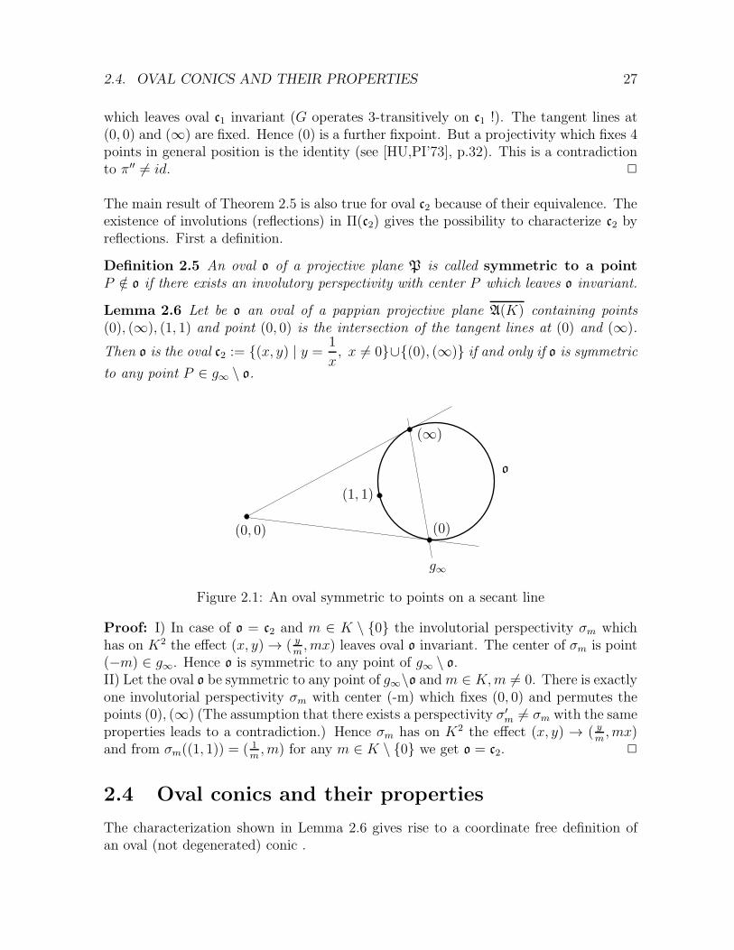
Definition 2.5 An oval o of a projective plane P is called symmetric to a pointP /∈ o if there exists an involutory perspectivity with center P which leaves o invariant.
Lemma 2.6 Let be o an oval of a pappian projective plane A(K) containing points(0), (∞), (1, 1) and point (0, 0) is the intersection of the tangent lines at (0) and (∞).
Then o is the oval c2 := {(x, y) | y =1
x, x 6= 0}∪{(0), (∞)} if and only if o is symmetric
to any point P ∈ g∞ \ o.
(∞)
(0)
(1, 1)
g∞
o
(0, 0)
Figure 2.1: An oval symmetric to points on a secant line
Proof: I) In case of o = c2 and m ∈ K \ {0} the involutorial perspectivity σm whichhas on K2 the effect (x, y) → ( y
m, mx) leaves oval o invariant. The center of σm is point
(−m) ∈ g∞. Hence o is symmetric to any point of g∞ \ o.II) Let the oval o be symmetric to any point of g∞\o andm ∈ K,m 6= 0. There is exactlyone involutorial perspectivity σm with center (-m) which fixes (0, 0) and permutes thepoints (0), (∞) (The assumption that there exists a perspectivity σ′
m 6= σm with the sameproperties leads to a contradiction.) Hence σm has on K2 the effect (x, y) → ( y
m, mx)
and from σm((1, 1)) = ( 1m, m) for any m ∈ K \ {0} we get o = c2. 2
2.4 Oval conics and their properties
The characterization shown in Lemma 2.6 gives rise to a coordinate free definition ofan oval (not degenerated) conic .
28 CHAPTER 2. OVALS AND CONICS
Definition 2.6 An oval o of a pappian projective plane is called oval conic if thefollowing property (SS) is given(SS) o is symmetric to any point P ∈ g \ o of a secant line g.
Because of Lemma 2.4 and Lemma 2.6 we get:
Lemma 2.7 For a projective plane A(K) the ovals c1, c2 and all their equivalent imagesare oval conics.
It makes no sense to extend the definition of an oval conic to arbitrary desarguesianplanes because for a non commutative skewfield K both point sets c1 (ARTZY [AR’71])and c2 (BERZ [BZ’62]) are no ovals in A(K). And a desarguesian planeP which containsan oval with the typical property (SS) is already pappian (see BUEKENHOUT [BU’69],4.5, MAURER [MA’81], 4.1).
Theorem 2.8 (projective equivalence of conics) Let P be a pappian projective plane.
a) For any three non collinear points U, V, E, any line u through U and any linev through v both different from UV , UE, V E there exists exactly one oval coniccontaining points U, V, E with tangent line u at point U and tangent line v at V .
b) Any two oval conics c, c′ of P are projectively equivalent.
Proof: a) P can be described as A(K) such that U = (0), V = (∞), E = (1, 1) andu ∩ v = {(0, 0)}. From Lemma 2.6 we get: The conic with properties assumed is c2.b) We describe P as A(K) such that c = c2. Let be g the secant line of c′ containingits points of symmetry and let be g ∩ c′ = {U, V } and u the tangent at U , v the tan-gent at V and E an arbitrary point of c \ {U, V }. There exists a projectivity π withπ(U) = (0), π(V ) = (∞), π(E) = (1, 1). Lemma 2.6 shows: π(c′) = c2 = c. 2
With the aid of Lemma 2.5 one proves the following statement.
Theorem 2.9 (symmetries of a conic) Let be c an oval conic of a pappian plane P
and K a coordinate field of P.
a) The group Π(c) of projectivities which leave c invariant is isomorphic to PGL(2, K).Π(c) operates sharply 3-transitive on c.
b) c is symmetric to any point P ∈ c which is in case of CharK = 2 different fromthe knot of c.
The importance of statement a) of the previous theorem shows the following result.
Result 2.10 (TITS [TI’62], 3.1) Let be o an oval of a pappian projective plane P
and Π(o) the group of projectivities which leave o invariant.
a) o is an oval conic if and only if Π(o) operates 3-transitively on o.
2.4. OVAL CONICS AND THEIR PROPERTIES 29
b) In case of a finite plane: o is an oval conic if and only if Π(o) operates 2-transitively on o.
For the proof of Theorem 2.12 we need the following statement which can be provedsimply by calculation.
Lemma 2.11 (quadrilateral on a hyperbola) Let K be a field and Pi = (xi, yi), i =1, .., 4 four points of the affine plane A(K) with xi 6= xk, yi 6= yk for i 6= k.The points P1, P2, P3, P4 lie on a hyperbola y = a
x−b+ c if and only if
(y4 − y1)(x4 − x2)
(x4 − x1)(y4 − y2)=
(y3 − y1)(x3 − x2)
(x3 − x1)(y3 − y2).
(See Section 5.3.3, too.)
The following theorems contain properties of ovals typical for conics.
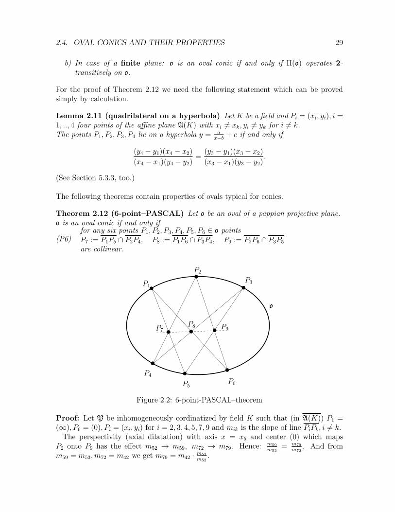
Theorem 2.12 (6-point–PASCAL) Let o be an oval of a pappian projective plane.o is an oval conic if and only if
(P6)for any six points P1, P2, P3, P4, P5, P6 ∈ o pointsP7 := P1P5 ∩ P2P4, P8 := P1P6 ∩ P3P4, P9 := P2P6 ∩ P3P5
are collinear.
P1
P2
P3
P4
P5P6
P7P8 P9
o
Figure 2.2: 6-point-PASCAL–theorem
Proof: Let P be inhomogeneously cordinatized by field K such that (in A(K)) P1 =(∞), P6 = (0), Pi = (xi, yi) for i = 2, 3, 4, 5, 7, 9 and mik is the slope of line PiPk, i 6= k.The perspectivity (axial dilatation) with axis x = x5 and center (0) which maps
P2 onto P9 has the effect m52 → m59, m72 → m79. Hence: m59
m52= m79
m72. And from
m59 = m53, m72 = m42 we get m79 = m42 ·m53
m52.
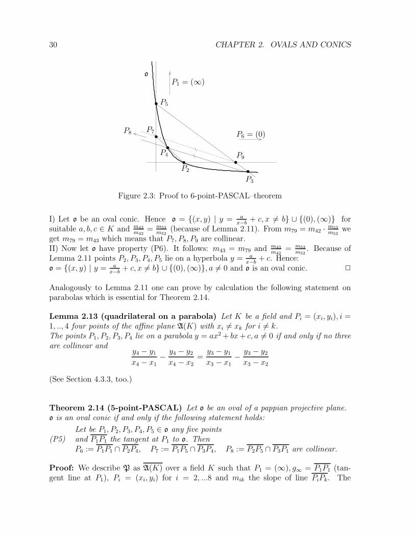
30 CHAPTER 2. OVALS AND CONICS
P1 = (∞)
P2
P3
P4
P5
P6 = (0)P7P8
P9
o
Figure 2.3: Proof to 6-point-PASCAL–theorem
I) Let o be an oval conic. Hence o = {(x, y) | y = ax−b
+ c, x 6= b} ∪ {(0), (∞)} forsuitable a, b, c ∈ K and m43
m42= m53
m52(because of Lemma 2.11). From m79 = m42 ·
m53
m52we
get m79 = m43 which means that P7, P8, P9 are collinear.II) Now let o have property (P6). It follows: m43 = m79 and m43
m42= m53
m52. Because of
Lemma 2.11 points P2, P3, P4, P5 lie on a hyperbola y = ax−b
+ c. Hence:o = {(x, y) | y = a
x−b+ c, x 6= b} ∪ {(0), (∞)}, a 6= 0 and o is an oval conic. 2
Analogously to Lemma 2.11 one can prove by calculation the following statement onparabolas which is essential for Theorem 2.14.
Lemma 2.13 (quadrilateral on a parabola) Let K be a field and Pi = (xi, yi), i =1, .., 4 four points of the affine plane A(K) with xi 6= xk for i 6= k.The points P1, P2, P3, P4 lie on a parabola y = ax2 + bx+ c, a 6= 0 if and only if no threeare collinear and
y4 − y1x4 − x1
−y4 − y2x4 − x2
=y3 − y1x3 − x1
−y3 − y2x3 − x2
(See Section 4.3.3, too.)
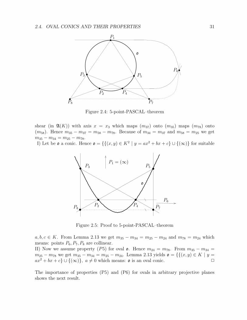
Theorem 2.14 (5-point-PASCAL) Let o be an oval of a pappian projective plane.o is an oval conic if and only if the following statement holds:
(P5)Let be P1, P2, P3, P4, P5 ∈ o any five pointsand P1P1 the tangent at P1 to o. ThenP6 := P1P1 ∩ P2P4, P7 := P1P5 ∩ P3P4, P8 := P2P5 ∩ P3P1 are collinear.
Proof: We describe P as A(K) over a field K such that P1 = (∞), g∞ = P1P1 (tan-gent line at P1), Pi = (xi, yi) for i = 2, ...8 and mik the slope of line PiPk. The
2.4. OVAL CONICS AND THEIR PROPERTIES 31
P1
P2
P3
P4
P5
P6
P7P8
o
Figure 2.4: 5-point-PASCAL–theorem
shear (in A(K)) with axis x = x3 which maps (m37) onto (m35) maps (m78) onto(m58). Hence m35 −m37 = m58 − m78. Because of m34 = m37 and m58 = m25 we getm35 −m34 = m25 −m78.I) Let be o a conic. Hence o = {{(x, y) ∈ K2 | y = ax2 + bx+ c} ∪ {(∞)} for suitable
P1 = (∞)
P2
P3
P4
P5
P6
P7P8
o
Figure 2.5: Proof to 5-point-PASCAL–theorem
a, b, c ∈ K. From Lemma 2.13 we get m35 − m34 = m25 − m24 and m78 = m24 whichmeans: points P6, P7, P8 are collinear.II) Now we assume property (P5) for oval o. Hence m24 = m78. From m35 − m34 =m25 −m78 we get m35 −m34 = m25 −m24. Lemma 2.13 yields o = {{(x, y) ∈ K | y =ax2 + bx+ c} ∪ {(∞)}, a 6= 0 which means: o is an oval conic. 2
The importance of properties (P5) and (P6) for ovals in arbitrary projective planesshows the next result.
32 CHAPTER 2. OVALS AND CONICS
Result 2.15 (BUEKENHOUT/HOFMANN) Let o be an oval of a projective planeP. The following statements are equivalent:
a) P is pappian and o an oval conic.
b) (P6) is true for oval o. (BUEKENHOUT [BU’66])
c) (P5) is true for oval o. (HOFMANN [HO’71])
For a pappian plane the degenerations (P4), (P3) ((P3) only in case of Char 6= 2)characterize oval conics, too. It is not clear if the assumption “pappian” can be omitted(see Result 2.15).
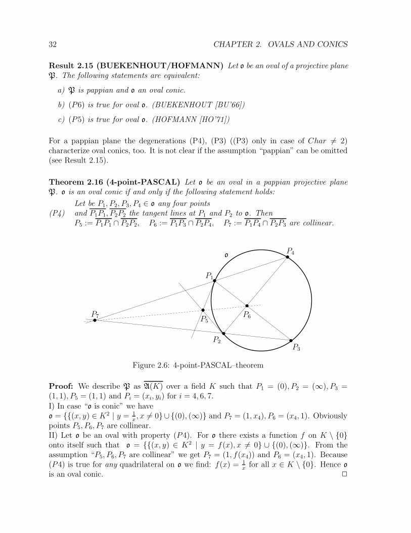
Theorem 2.16 (4-point-PASCAL) Let o be an oval in a pappian projective planeP. o is an oval conic if and only if the following statement holds:
(P4)Let be P1, P2, P3, P4 ∈ o any four pointsand P1P1, P2P2 the tangent lines at P1 and P2 to o. ThenP5 := P1P1 ∩ P2P2, P6 := P1P3 ∩ P2P4, P7 := P1P4 ∩ P2P3 are collinear.
P1
P2P3
P4
P5P6P7
o
Figure 2.6: 4-point-PASCAL–theorem
Proof: We describe P as A(K) over a field K such that P1 = (0), P2 = (∞), P3 =(1, 1), P5 = (1, 1) and Pi = (xi, yi) for i = 4, 6, 7.
I) In case “o is conic” we haveo = {{(x, y) ∈ K2 | y = 1
x, x 6= 0}∪{(0), (∞)} and P7 = (1, x4), P6 = (x4, 1). Obviously
points P5, P6, P7 are collinear.II) Let o be an oval with property (P4). For o there exists a function f on K \ {0}onto itself such that o = {{(x, y) ∈ K2 | y = f(x), x 6= 0} ∪ {(0), (∞)}. From theassumption “P5, P6, P7 are collinear” we get P7 = (1, f(x4)) and P6 = (x4, 1). Because(P4) is true for any quadrilateral on o we find: f(x) = 1
xfor all x ∈ K \ {0}. Hence o
is an oval conic. 2
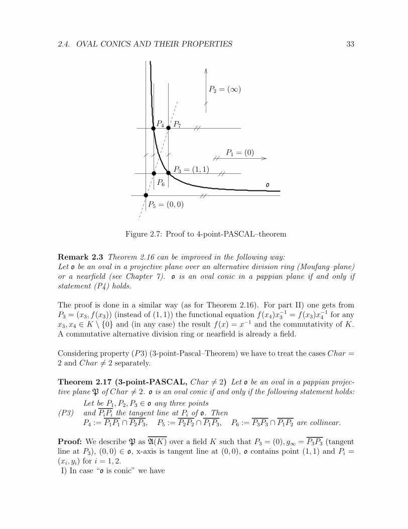
2.4. OVAL CONICS AND THEIR PROPERTIES 33
P1 = (0)
P2 = (∞)
P3 = (1, 1)
P4
P5 = (0, 0)
P6
P7
o
Figure 2.7: Proof to 4-point-PASCAL–theorem
Remark 2.3 Theorem 2.16 can be improved in the following way:Let o be an oval in a projective plane over an alternative division ring (Moufang–plane)or a nearfield (see Chapter 7). o is an oval conic in a pappian plane if and only ifstatement (P4) holds.
The proof is done in a similar way (as for Theorem 2.16). For part II) one gets fromP3 = (x3, f(x3)) (instead of (1, 1)) the functional equation f(x4)x
−13 = f(x3)x
−14 for any
x3, x4 ∈ K \ {0} and (in any case) the result f(x) = x−1 and the commutativity of K.A commutative alternative division ring or nearfield is already a field.
Considering property (P3) (3-point-Pascal–Theorem) we have to treat the cases Char =2 and Char 6= 2 separately.
Theorem 2.17 (3-point-PASCAL, Char 6= 2) Let o be an oval in a pappian projec-tive plane P of Char 6= 2. o is an oval conic if and only if the following statement holds:
(P3)Let be P1, P2, P3 ∈ o any three pointsand PiPi the tangent line at Pi of o. ThenP4 := P1P1 ∩ P2P3, P5 := P2P2 ∩ P1P3, P6 := P3P3 ∩ P1P2 are collinear.
Proof: We describe P as A(K) over a field K such that P3 = (0), g∞ = P3P3 (tangentline at P3), (0, 0) ∈ o, x-axis is tangent line at (0, 0), o contains point (1, 1) and Pi =(xi, yi) for i = 1, 2.I) In case “o is conic” we have
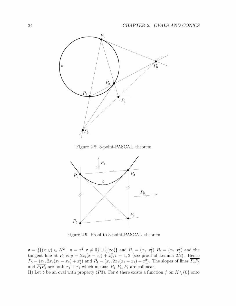
34 CHAPTER 2. OVALS AND CONICS
P1
P2
P3
P4
P5
P6o
Figure 2.8: 3-point-PASCAL–theorem
P1P2
P3
P4
P5
P6
o
Figure 2.9: Proof to 3-point-PASCAL–theorem
o = {{(x, y) ∈ K2 | y = x2, x 6= 0} ∪ {(∞)} and P1 = (x1, x21), P2 = (x2, x
22) and the
tangent line at Pi is y = 2xi(x − xi) + x2i , i = 1, 2 (see proof of Lemma 2.2). HenceP5 = (x1, 2x2(x1 − x2) + x22) and P4 = (x2, 2x1(x2 − x1) + x21). The slopes of lines P4P5
and P1P2 are both x1 + x2 which means: P4, P5, P6 are collinear.II) Let o be an oval with property (P3). For o there exists a function f on K \ {0} onto
2.4. OVAL CONICS AND THEIR PROPERTIES 35
itself such that o = {{(x, y) ∈ K2 | y = f(x), x 6= 0} ∪ {(∞)}. The tangent line at(x0, f(x0)) has equation y = f ′(x0)(x− x0) + f(x0). Hence: P5 = (x1, f
′(x2)(x1 − x2) +f(x2)) and P4 = (x2, f
′(x1)(x2 − x1) + f(x1)). Because of property (P3) the slopes of
the lines P4, P5 and P1, P2 are equal and we get at first f ′(x2) + f ′(x1) −f(x2)−f(x1)
x2−x1=
f(x2)−f(x1)x2−x1
and herefrom the functional equation:(i): (f ′(x2) + f ′(x1))(x2 − x1) = 2(f(x2)− f(x1)) for any x1, x2 ∈ K.With f(0) = f ′(0) = 0 we get (ii): f ′(x2)x2 = 2f(x2) and f(1) = 1 yields (iii):f ′(1) = 2. From (i) and (ii) follows (iv): f ′(x2)x1 = f ′(x1)x2 and, using (iii), we find(v): f ′(x2) = 2x2 for any x2 ∈ K. From (ii) and (v) we get f(x2) = x22, x2 ∈ K whichmeans: o is an oval conic. 2
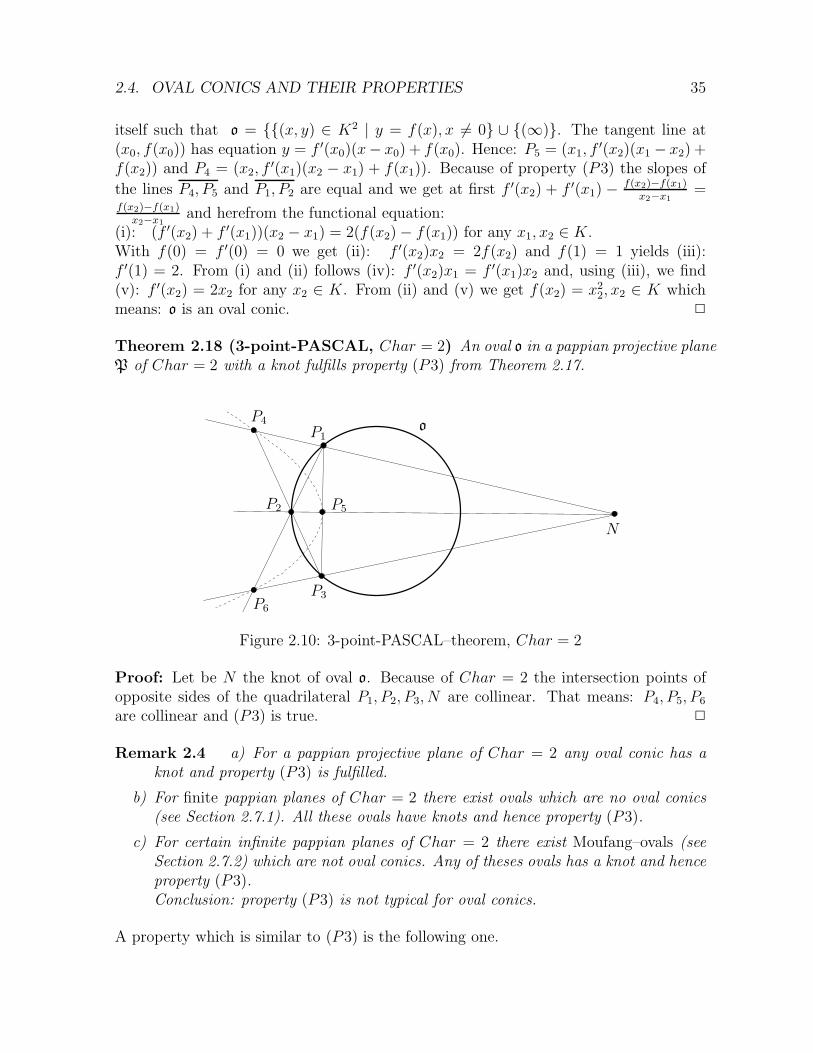
Theorem 2.18 (3-point-PASCAL, Char = 2) An oval o in a pappian projective planeP of Char = 2 with a knot fulfills property (P3) from Theorem 2.17.
P1
P2
P3
P4
P5
P6
N
o
Figure 2.10: 3-point-PASCAL–theorem, Char = 2
Proof: Let be N the knot of oval o. Because of Char = 2 the intersection points ofopposite sides of the quadrilateral P1, P2, P3, N are collinear. That means: P4, P5, P6
are collinear and (P3) is true. 2
Remark 2.4 a) For a pappian projective plane of Char = 2 any oval conic has aknot and property (P3) is fulfilled.
b) For finite pappian planes of Char = 2 there exist ovals which are no oval conics(see Section 2.7.1). All these ovals have knots and hence property (P3).
c) For certain infinite pappian planes of Char = 2 there exist Moufang–ovals (seeSection 2.7.2) which are not oval conics. Any of theses ovals has a knot and henceproperty (P3).Conclusion: property (P3) is not typical for oval conics.
A property which is similar to (P3) is the following one.
36 CHAPTER 2. OVALS AND CONICS
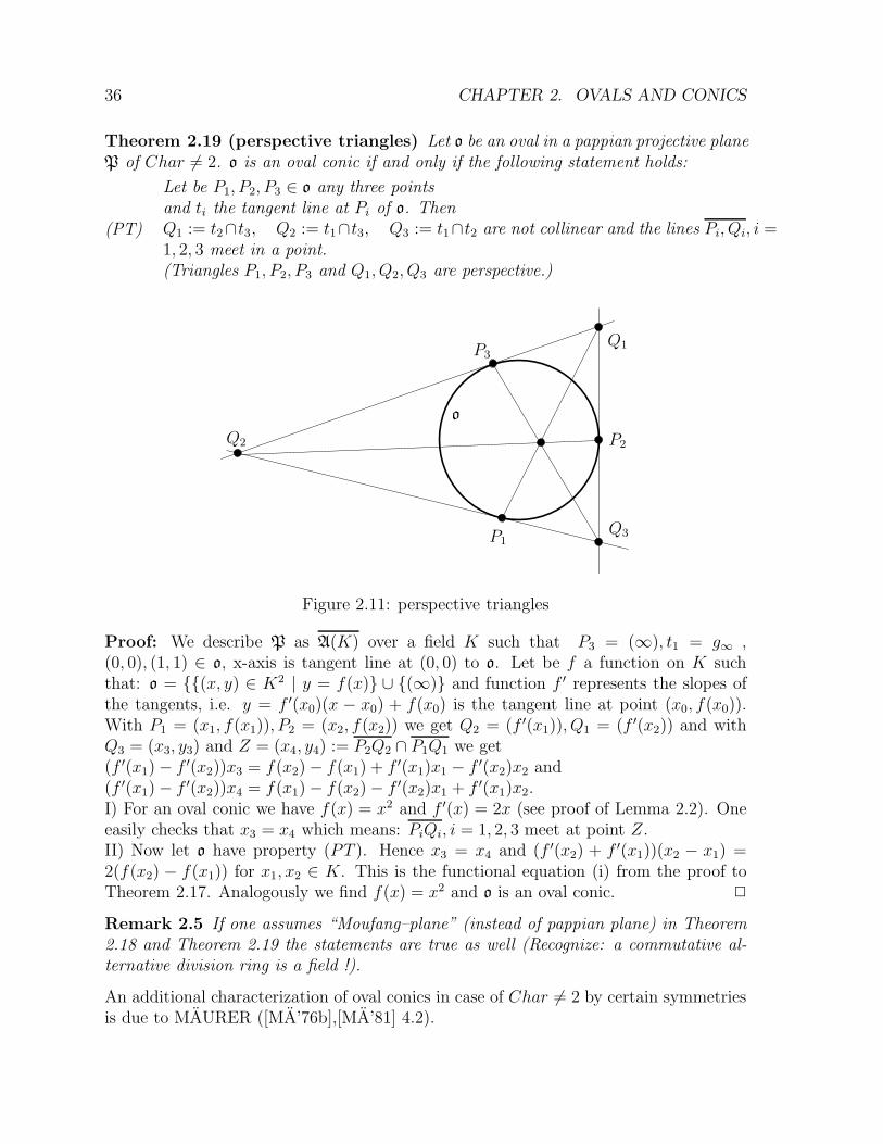
Theorem 2.19 (perspective triangles) Let o be an oval in a pappian projective planeP of Char 6= 2. o is an oval conic if and only if the following statement holds:
(PT)
Let be P1, P2, P3 ∈ o any three pointsand ti the tangent line at Pi of o. ThenQ1 := t2∩t3, Q2 := t1∩t3, Q3 := t1∩t2 are not collinear and the lines Pi, Qi, i =1, 2, 3 meet in a point.(Triangles P1, P2, P3 and Q1, Q2, Q3 are perspective.)
P1
P2
P3Q1
Q2
Q3
o
Figure 2.11: perspective triangles
Proof: We describe P as A(K) over a field K such that P3 = (∞), t1 = g∞ ,(0, 0), (1, 1) ∈ o, x-axis is tangent line at (0, 0) to o. Let be f a function on K suchthat: o = {{(x, y) ∈ K2 | y = f(x)} ∪ {(∞)} and function f ′ represents the slopes ofthe tangents, i.e. y = f ′(x0)(x − x0) + f(x0) is the tangent line at point (x0, f(x0)).With P1 = (x1, f(x1)), P2 = (x2, f(x2)) we get Q2 = (f ′(x1)), Q1 = (f ′(x2)) and withQ3 = (x3, y3) and Z = (x4, y4) := P2Q2 ∩ P1Q1 we get(f ′(x1)− f ′(x2))x3 = f(x2)− f(x1) + f ′(x1)x1 − f ′(x2)x2 and(f ′(x1)− f ′(x2))x4 = f(x1)− f(x2)− f ′(x2)x1 + f ′(x1)x2.I) For an oval conic we have f(x) = x2 and f ′(x) = 2x (see proof of Lemma 2.2). Oneeasily checks that x3 = x4 which means: PiQi, i = 1, 2, 3 meet at point Z.II) Now let o have property (PT ). Hence x3 = x4 and (f ′(x2) + f ′(x1))(x2 − x1) =2(f(x2) − f(x1)) for x1, x2 ∈ K. This is the functional equation (i) from the proof toTheorem 2.17. Analogously we find f(x) = x2 and o is an oval conic. 2
Remark 2.5 If one assumes “Moufang–plane” (instead of pappian plane) in Theorem2.18 and Theorem 2.19 the statements are true as well (Recognize: a commutative al-ternative division ring is a field !).
An additional characterization of oval conics in case of Char 6= 2 by certain symmetriesis due to MAURER ([MA’76b],[MA’81] 4.2).
2.4. OVAL CONICS AND THEIR PROPERTIES 37
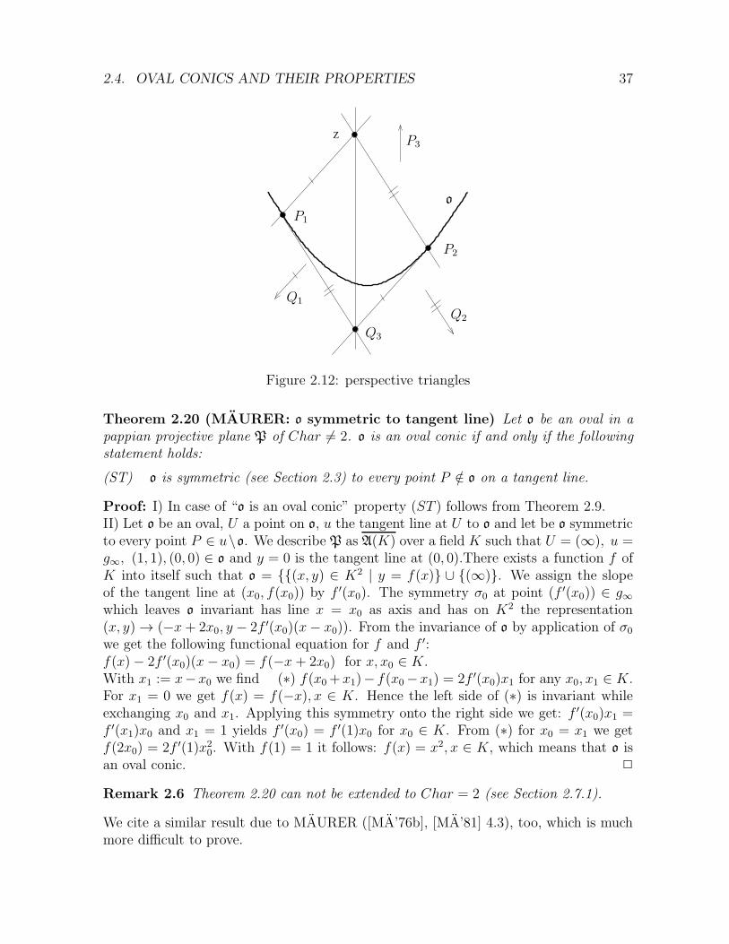
Z
P1
P2
P3
Q1
Q2
Q3
o
Figure 2.12: perspective triangles
Theorem 2.20 (MAURER: o symmetric to tangent line) Let o be an oval in apappian projective plane P of Char 6= 2. o is an oval conic if and only if the followingstatement holds:
(ST) o is symmetric (see Section 2.3) to every point P /∈ o on a tangent line.
Proof: I) In case of “o is an oval conic” property (ST ) follows from Theorem 2.9.II) Let o be an oval, U a point on o, u the tangent line at U to o and let be o symmetricto every point P ∈ u\o. We describe P as A(K) over a field K such that U = (∞), u =g∞, (1, 1), (0, 0) ∈ o and y = 0 is the tangent line at (0, 0).There exists a function f ofK into itself such that o = {{(x, y) ∈ K2 | y = f(x)} ∪ {(∞)}. We assign the slopeof the tangent line at (x0, f(x0)) by f ′(x0). The symmetry σ0 at point (f ′(x0)) ∈ g∞which leaves o invariant has line x = x0 as axis and has on K2 the representation(x, y) → (−x+ 2x0, y − 2f ′(x0)(x− x0)). From the invariance of o by application of σ0we get the following functional equation for f and f ′:f(x)− 2f ′(x0)(x− x0) = f(−x+ 2x0) for x, x0 ∈ K.With x1 := x−x0 we find (∗) f(x0+x1)− f(x0−x1) = 2f ′(x0)x1 for any x0, x1 ∈ K.For x1 = 0 we get f(x) = f(−x), x ∈ K. Hence the left side of (∗) is invariant whileexchanging x0 and x1. Applying this symmetry onto the right side we get: f ′(x0)x1 =f ′(x1)x0 and x1 = 1 yields f ′(x0) = f ′(1)x0 for x0 ∈ K. From (∗) for x0 = x1 we getf(2x0) = 2f ′(1)x20. With f(1) = 1 it follows: f(x) = x2, x ∈ K, which means that o isan oval conic. 2
Remark 2.6 Theorem 2.20 can not be extended to Char = 2 (see Section 2.7.1).
We cite a similar result due to MAURER ([MA’76b], [MA’81] 4.3), too, which is muchmore difficult to prove.
38 CHAPTER 2. OVALS AND CONICS
Result 2.21 (MAURER: o symmetric to exterior line) Let o be an oval in a pap-pian projective plane P of Char 6= 2. o is an oval conic if and only if the followingstatement holds:
(SP) o is symmetric (see Section 2.3) to any point P on an exterior line.
At least we give the STEINER–characterization of oval conics which is commonly usedfor its definition.
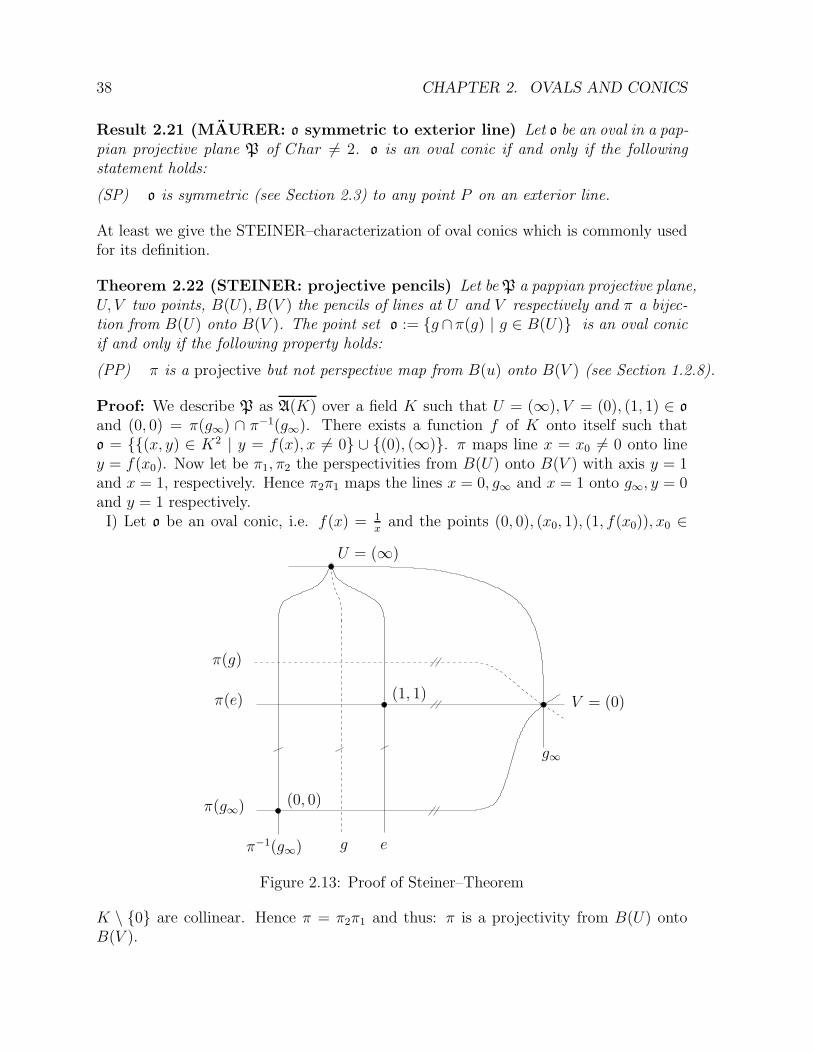
Theorem 2.22 (STEINER: projective pencils) Let be P a pappian projective plane,U, V two points, B(U), B(V ) the pencils of lines at U and V respectively and π a bijec-tion from B(U) onto B(V ). The point set o := {g ∩ π(g) | g ∈ B(U)} is an oval conicif and only if the following property holds:
(PP) π is a projective but not perspective map from B(u) onto B(V ) (see Section 1.2.8).
Proof: We describe P as A(K) over a field K such that U = (∞), V = (0), (1, 1) ∈ o
and (0, 0) = π(g∞) ∩ π−1(g∞). There exists a function f of K onto itself such thato = {{(x, y) ∈ K2 | y = f(x), x 6= 0} ∪ {(0), (∞)}. π maps line x = x0 6= 0 onto liney = f(x0). Now let be π1, π2 the perspectivities from B(U) onto B(V ) with axis y = 1and x = 1, respectively. Hence π2π1 maps the lines x = 0, g∞ and x = 1 onto g∞, y = 0and y = 1 respectively.I) Let o be an oval conic, i.e. f(x) = 1
xand the points (0, 0), (x0, 1), (1, f(x0)), x0 ∈
π(g)
π(g∞)
g∞
π(e)
(0, 0)
(1, 1)
π−1(g∞)
U = (∞)
V = (0)
g e
Figure 2.13: Proof of Steiner–Theorem
K \ {0} are collinear. Hence π = π2π1 and thus: π is a projectivity from B(U) ontoB(V ).
2.5. OVAL CONICS IN AFFINE PLANES 39
II) Let π be a perspectivity from B(U) onto B(V ). Because both π and π2π1 have thesame effect on the lines x = 0, g∞ and x = 1 we get from Result 1.17 e) that π = π2π1.Hence points (0, 0), (x0, 1), (1, f(x0)) are collinear for any x0 ∈ K \ {0} and thereforef(x0) =
1x0
which means: o is an oval conic. 2
Remark 2.7 The second classical definition of a conic is due to v. STAUDT which usesthe term “polarity” (see LENZ [LE’65]). Because the definition via a polarity yields onlyan oval in case of Char 6= 2 (see BERZ [BZ’62]) we omit it here.
2.5 Oval conics in affine planes
Let be P be a pappian projective plane and P(K) the homogeneous model of P over afield K (see Section 1.2.4) and let be c the oval conic in P(K) with equation x21 = x2x3(see Section 2.3). We shall discuss the question when there is a line g∞ such thatc ∩ g∞ = ∅. Hence c is an oval in the affine plane with g∞ as line at infinity.
Let be g∞ a line of P(K) with equation ax1 + bx2 + cx3 = 0 and c ∩ g∞ = ∅. From< (0, 1, 0) >,< (0, 0, 1) >∈ c we get b 6= 0, c 6= 0 and the equation ax1x2+ bx
22+ cx
21 = 0
has only the solution (0, 0, 0) which means: polynom cξ2 + aξ + b is irreducible over K.(The reverse is also true: If cξ2+aξ+ b is irreducible over K then line g∞ with equationax1 + bx2 + cx3 = 0 and oval c have no points in common.) We set c = 1 and performthe coordinate transformation x′1 = x1, x
′2 = x2, x
′3 = ax1 + bx2 + x3. Hence g∞ has
equation x′3 = 0 and conic c the equation x′12+ax′1x
′2+bx
′22−x′2x
′3 = 0. After introducing
inhomogeneous coordinates with x =x′
1
x′
3
, y =x′
2
x′
3
equation x2+axy+by2−y = 0 describes
an oval in A(K). This proves the following theorem.
Theorem 2.23 (oval conic in A(K)) Let be K a field.The point set o = {(x, y) | x2+ axy+ by2− y = 0} for a, b ∈ K is an oval in the affineplane A(K) if and only if polynom ξ2 + aξ + b is irreducible over K.
From Theorem 2.23 and a suitable coordinate transformation for A(K) we get thefollowing special results.
Theorem 2.24 (special affine oval conics) Let be K a field.
a) The point set o = {(x, y) | x2 + axy + y2 = 1} for a ∈ K is an oval in the affineplane A(K) if and only if polynom ξ2 + aξ + 1 is irreducible over K.
b) In case of Char = 2 point set o = {(x, y) | x2 + by2 + y = 0} for b ∈ K is anoval in the affine plane A(K) if and only if b is no square. The tangent lines of oare parallel to the x-axis, i.e. the knot of o in A(K) is point (0).
Remark 2.8 a) For K = GF (2) polynom ξ2 + ξ + 1 is irreducible.
b) For K = GF (q) number −1 is no square if and only if q ≡ 3 mod 4. Henceequation x2 + y2 = 1 describes an oval in A(GF (q)) if and only if q ≡ 3 mod 4.
40 CHAPTER 2. OVALS AND CONICS
c) ForK = IQ polynom ξ2−2 (for example) is irreducible. Hence equation x2−2y2 = 1describes an oval in A(IQ) (but not in A(IR) !).
2.6 Finite ovals
Here we collect some properties typical for finite ovals.
Theorem 2.25 (set of n+ 1 points) Let be P a projective plane of order n.A set o of points is an oval if |o| = n+ 1 and if no three points of o are collinear.
Proof: I) If o is an oval no three points are collinear (see definition of an oval). Becausefor any point P ∈ o there is exactly one tangent line we have n secant lines throughpoint P which meet o in exactly one additional point. Hence |o| = n + 1.II) Let be o a set of n+1 points with “no three collinear”. For any point P ∈ o there areexactly n lines through P which have exactly one additional point with o in common.Hence there is exactly one line tP through P with |tP ∩ o| = 1 and o is an oval. 2
Theorem 2.26 (QVIST [QV’52]) Let be P a projective plane of order n and o anoval in P.a) If n is odd any point P /∈ o lies on 0 or 2 tangent lines.b) In case of “n is even” oval o has a complete knot, i.e. there exists a point N whichlies on all tangent lines of oval o and any line through N is a tangent line.
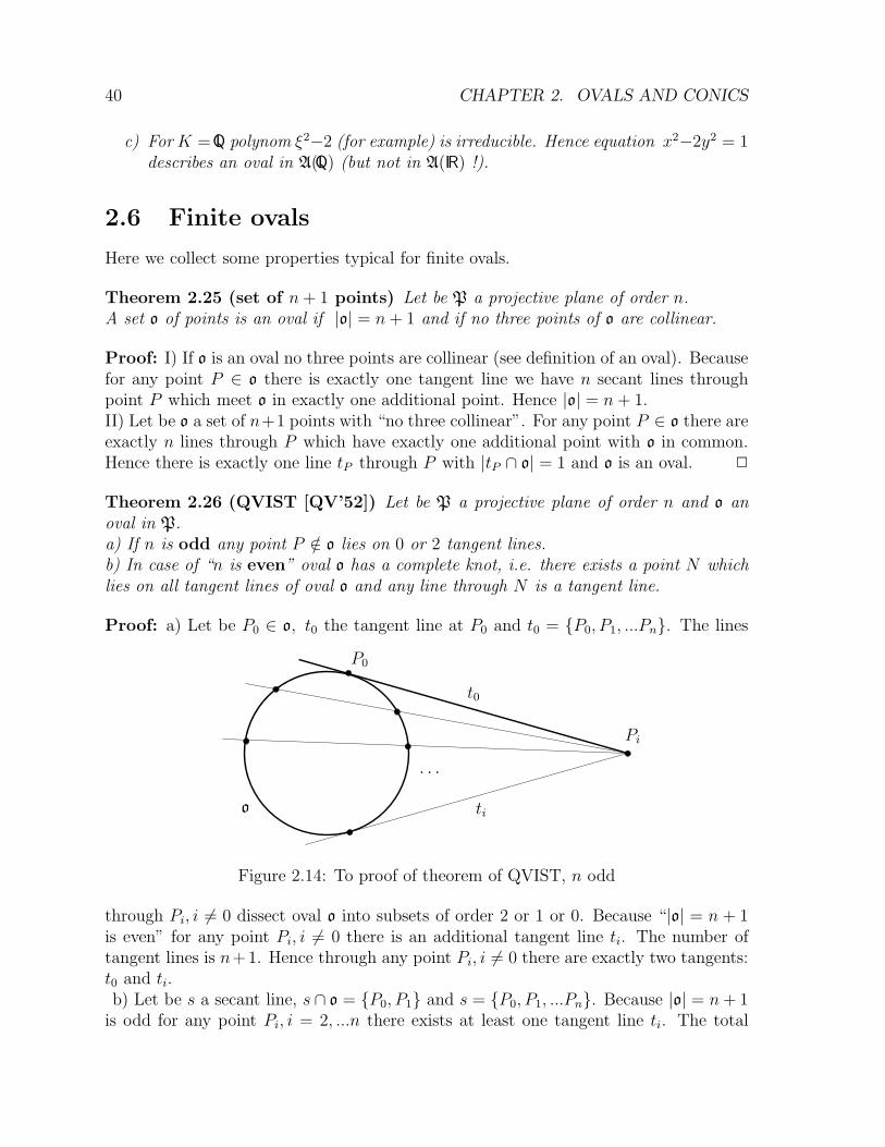
Proof: a) Let be P0 ∈ o, t0 the tangent line at P0 and t0 = {P0, P1, ...Pn}. The lines
P0
Pi
t0
tio
· · ·
Figure 2.14: To proof of theorem of QVIST, n odd
through Pi, i 6= 0 dissect oval o into subsets of order 2 or 1 or 0. Because “|o| = n + 1is even” for any point Pi, i 6= 0 there is an additional tangent line ti. The number oftangent lines is n+1. Hence through any point Pi, i 6= 0 there are exactly two tangents:t0 and ti.b) Let be s a secant line, s ∩ o = {P0, P1} and s = {P0, P1, ...Pn}. Because |o| = n+ 1is odd for any point Pi, i = 2, ...n there exists at least one tangent line ti. The total
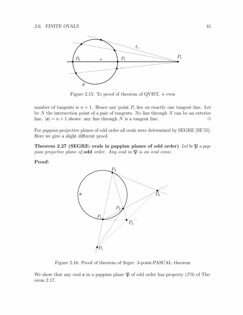
2.6. FINITE OVALS 41
...
P0 P1Pis
ti
o
Figure 2.15: To proof of theorem of QVIST, n even
number of tangents is n + 1. Hence any point Pi lies on exactly one tangent line. Letbe N the intersection point of a pair of tangents. No line through N can be an exteriorline. |o| = n + 1 shows: any line through N is a tangent line. 2
For pappian projective planes of odd order all ovals were determined by SEGRE [SE’55].Here we give a slight different proof.
Theorem 2.27 (SEGRE: ovals in pappian planes of odd order) Let be P a pap-pian projective plane of odd order. Any oval in P is an oval conic.
Proof:
P1
P2
P3
P4
P5
P6o
Figure 2.16: Proof of theorem of Segre: 3-point-PASCAL–theorem
We show that any oval o in a pappian plane P of odd order has property (P3) of The-orem 2.17.

42 CHAPTER 2. OVALS AND CONICS
P1 = (1, 1)
P2 = (0)
P3 = (∞)
P = (x, f(x))
P5 = (1, 0)
P6 = (0, 1)
o
Figure 2.17: Proof of theorem of SEGRE: o coordinatized inhomogeneously
Let be P1, P2, P3 an arbitrary triangle on o and P4, P5, P6 defined as in Theorem 2.17.We describe P as A(K) over K = GF (n) such that P3 = (∞), P2 = (0), P1 = (1, 1) and(0, 0) is the intersection point of the tangent lines at P2 and P3. Hence P5 = (1, 0) andP6 = (0, 1). Oval o can be described by a bijective function f from K \ {0} onto itself:o = {(x, y) ∈ K2 | y = f(x), x 6= 0} ∪ {(0), (∞)}.
For point P = (x, f(x)), x ∈ K \ {0, 1} the slope of the line PP1 is m(x) = f(x)−1x−1
.Both mappings x → f(x) − 1 and x → x − 1 are bijections from K \ {0, 1} ontoK \ {0,−1} and hence x → m(x) is a bijection from K \ {0, 1} onto K \ {0, m1} wherem1 is the slope of the tangent line at P1. With the abbreviation K∗∗ := K\{0, 1} we get:
∏
x∈K∗∗
(f(x)− 1) =∏
x∈K∗∗
(x− 1) = 1 and m1 ·∏
x∈K∗∗
f(x)− 1
x− 1= −1.
(Recognize: For K∗ := K \ {0} we have:∏
x∈K∗
k = −1.) Hence
−1 = m1 ·∏
x∈K∗∗
f(x)− 1
x− 1= m1 ·
∏
x∈K∗∗
(f(x)− 1)
∏
x∈K∗∗
(x− 1)= m1.
Because both the slopes of P5P6 and tangent P1P1 are −1 we get P1P1 ∩ P2P3 = P4 ∈P5P6. This is true for any triangle P1, P2, P3 ∈ o. Theorem 2.17 proves: o is an ovalconic. 2
2.7. FURTHER EXAMPLES OF OVALS 43
Additional finite ovals are contained in Section 2.7 especially ovals in desarguesian planesof even order which are no oval conics.
2.7 Further examples of ovals
2.7.1 Translation–ovals
Definition 2.7 Let be P a projective plane, o an oval in P, t a tangent line of o andE(o, t) the set of elations with axis t which leave o invariant. o is called translation–oval if the following property holds:
(TO) There is a tangent line t0 of o such that E(o, t0) operates transitively on o \ t0.
It follows directly from the definition:
Lemma 2.28 Any translation–oval has a knot.
Example 2.3 a) The simplest examples are oval conics in a pappian plane of Char = 2:For a field K with CharK = 2 the point seto := {(x, y) | y = x2} ∪ {(∞)} in A(K) is a translation–oval. The set E(o, g∞) of ela-tions are translations in A(K) of the following form: (x, y) → (x+ x0, y + x20), x0 ∈ Kand operates transitively on o \ t0.b) If one exchanges the knot of an oval from examples a) with an arbitrary point of oone gets a further translation–oval:For a field K with CharK = 2 the point seto := {(x, y) | y = x2} ∪ {(0)} in A(K) is a translation–oval (see Theorem 2.3).c) Let be K = GF (2n) ando(k) := {(x, y) | y = x2
k
}∪{(∞)} where k ∈ {1, ..., n−1} and k and n have no commondivisor. Then: o is a translation–oval in A(K). (see SEGRE [SE’57], DEMBOWSKI[DE’68], p. 51).
The importance of examples c) shows the following result.
Result 2.29 (PAYNE [PA’71]) Any translation–oval in a desarguesian plane A(K)over a field K = GF (2n) is equivalent to an oval o(k) of examples c) above.
Remark 2.9 Until now (1984) examples c) above are the only ovals known in A(K)for GF (2n).
Further examples of translation–ovals are contained in the following section.
44 CHAPTER 2. OVALS AND CONICS
2.7.2 Moufang–ovals
Definition 2.8 Let be P a projective plane, o an oval in P, t a tangent line of o andE(o, t) the set of elations with axis t which leave o invariant. o is called Moufang–ovalif the following property holds.
(MO)There are two tangent lines t1, t2 of o such that E(o, t1) and E(o, t1) operatetransitively on o \ t1 and o \ t2 respectively.
From the definition we recognize: any Moufang–oval is a translation–oval and the state-ments in the following lemma are true.
Lemma 2.30 a) Any Moufang–oval has a knot.b) Let o be a Moufang–oval and t an arbitrary tangent line of o. Then the set E(o, t) ofelations operates transitively on o \ t.
The following result is a construction tool for Moufang–ovals.
Result 2.31 (HARTMANN [HA’81c]) Let K be a skewfield and f an injectivefunction from K into itself with f(0) = 0, f(1) = 1.o = {(x, y) ∈ K2 | y = f(x)} ∪ {(∞)} is a Moufang–oval in A(K) if and only if(i) f(x1+x2) = f(x1)+f(x2), x1, x2 ∈ K, (ii) f(xf(x)−1) = f(x)−1, x ∈ K \{0}.
Example 2.4 Due to result 2.31 one has to find suitable skewfields and functions withproperties (i),(ii).
a) Let be K0 a field with CharK = 2 and K := K0(t) a transcendental expansion ofK0. Then L := K0(t
2) is a subfield of K and any x ∈ K can be written as x = ξ+ηtwith ξ, η ∈ L. Furthermore L2 := {x2|x ∈ L} is a subfield of L. Hence L is avector space over L2. For any element α ∈ L \ L2 function f : ξ + ηt → ξ2 + αη2
fulfills conditions (i) and (ii) of Result 2.31 (see TITS [TI’62] 2.4.). (For α = t2
we get f(x) = x2 and o is an oval conic.)
b) Let be K0 a field with CharK = 2 and there exists an involutorial automorphismσ of K0. K := K(t; σ) is the skewfield with kt = tkσ, k ∈ K0 (see COHN [CO’77],p.441). Then L = K0(t
2) is a commutative subskewfield of K. Any element of Kcan be written as ξ+ tη, ξ, η ∈ L. Function f : ξ+ tη → ξ2+ t2η2 fulfills conditions(i) and (ii) of Result 2.31 (see HARTMANN [HA’81c]).
c) HARTMANN [HA’81c] contains Moufang–ovals in non desarguesian Moufangplanes, too.
For finite Moufang–ovals we have:
Result 2.32 (TITS [TI’62]) Any Moufang–oval of a finite desarguesian plane is anoval conic. (see also [HA’81c])
2.7. FURTHER EXAMPLES OF OVALS 45
2.7.3 Ovals in Moulton–planes
Let be K an euclidean field, i.e. K is ordered and any positive element is a square, andk ∈ K, k > 0. We define on K a new multiplication ◦:
a ◦ b :=
{
kab , a, b < 0ab , other cases
Hence P := (P,G,∈) withP := K2 ∪ K ∪ {∞}, ∞ /∈ K,G = {{(x, y) ∈ K2 | y = m ◦ x+ b} ∪ {(m)} | m, b ∈ K}
∪ {{(x, y) ∈ P | x = c} ∪ {(∞)} | c ∈ K}∪ {(m) |m ∈ K ∪ {(∞)}.
is a projective Moulton–plane ando := {(x, y) | y = x ◦ x} ∪ {(∞)} is an oval in P (see [HA’76]).
2.7.4 Ovals in planes over nearfields
Let be (K,+, ·, f) a planar Tits-nearfield (see Section 7.5). Then P := (P,G,∈) withP := K2 ∪ K ∪ {∞}, ∞ /∈ K,G = {{(x, y) ∈ K2 | y = mx+ b} ∪ {(m)} | m, b ∈ K}
∪ {{(x, y) ∈ P | x = c} ∪ {(c)} | c ∈ K}∪ {(m) |m ∈ K ∪ {(∞)}.
is a projective plane ando := {(x, y) | y = f(x), x 6= 0} ∪ {(0), (∞)} is an oval in P (see Section 6.3).
2.7.5 Ovals in finite planes over quasifields
Let be K = GL(pn) with p > 2 and n ≥ 1. We define a new multiplication ◦:
a ◦ b :=
{
ab , a is a squareabp , a is no square
Then (K,+, ◦) is an ANDRE–quasifield (see [HU,PI’73], p. 187) and P = (P,G,∈)withP := K2 ∪ K ∪ {∞}, ∞ /∈ K,G = {{(x, y) ∈ K2 | y = m ◦ x+ b} ∪ {(m)} | m, b ∈ K}
∪ {{(x, y) ∈ P | x = c} ∪ {(∞)} | c ∈ K}∪ {(m) |m ∈ K ∪ {(∞)}.
is a projective plane ando := {(x, y) | y = 1
x, x 6= 0} ∪ {(0), (∞)} ( 1
xis the inverse of x with respect of the field
multiplication) is an oval in P.
Remark 2.10 a) For n = 1 we have (K,+, ◦) = (K,+, ·) and o is an oval conic.
46 CHAPTER 2. OVALS AND CONICS
b) For n = 2 (K,+, ◦) is a Tits–nearfield and o an example given in Section 2.7.4.
c) For n ≥ 3 (K,+, ◦) is a non associative quasifield.
2.7.6 Real ovals on convex functions
Let be f : IR → IR a convex function (see [RO,VA’73]) with properties(i) f is differentiable,(ii) f ′ is a strongly monotone increasing bijection of IR.Then o := {(x, y) | y = f(x)} ∪ {(∞)} is an oval in A(IR) (see [HA’84]).
Chapter 3
MOEBIUS–PLANES
Literature: [BE’73], [BP’83], [DE’68], [EW’71]
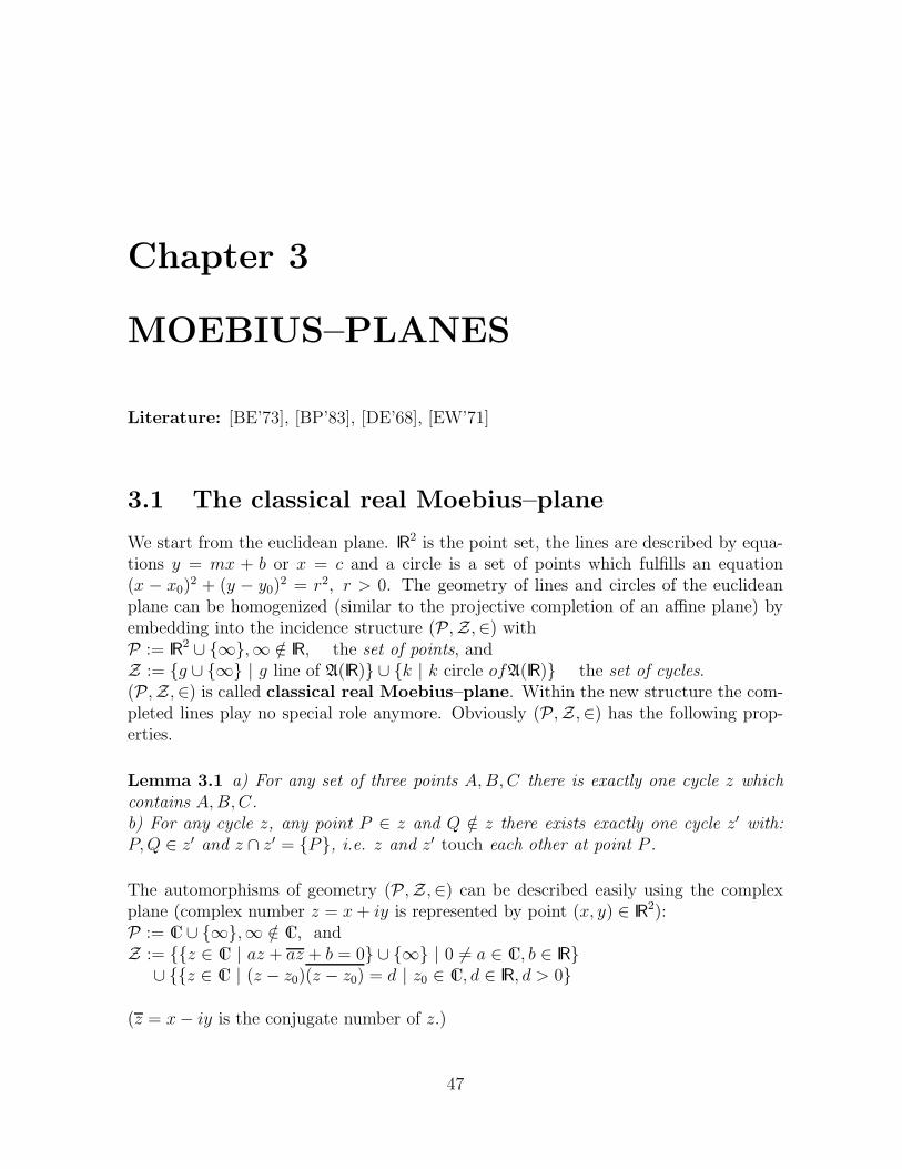
3.1 The classical real Moebius–plane
We start from the euclidean plane. IR2 is the point set, the lines are described by equa-tions y = mx + b or x = c and a circle is a set of points which fulfills an equation(x − x0)
2 + (y − y0)2 = r2, r > 0. The geometry of lines and circles of the euclidean
plane can be homogenized (similar to the projective completion of an affine plane) byembedding into the incidence structure (P,Z,∈) withP := IR
2 ∪ {∞},∞ /∈ IR, the set of points, andZ := {g ∪ {∞} | g line of A(IR)} ∪ {k | k circle ofA(IR)} the set of cycles.(P,Z,∈) is called classical real Moebius–plane. Within the new structure the com-pleted lines play no special role anymore. Obviously (P,Z,∈) has the following prop-erties.
Lemma 3.1 a) For any set of three points A,B,C there is exactly one cycle z whichcontains A,B,C.b) For any cycle z, any point P ∈ z and Q /∈ z there exists exactly one cycle z′ with:P,Q ∈ z′ and z ∩ z′ = {P}, i.e. z and z′ touch each other at point P .
The automorphisms of geometry (P,Z,∈) can be described easily using the complexplane (complex number z = x+ iy is represented by point (x, y) ∈ IR
2):P := C ∪ {∞},∞ /∈ C, andZ := {{z ∈ C | az + az + b = 0} ∪ {∞} | 0 6= a ∈ C, b ∈ IR}
∪ {{z ∈ C | (z − z0)(z − z0) = d | z0 ∈ C, d ∈ IR, d > 0}
(z = x− iy is the conjugate number of z.)
47
48 CHAPTER 3. MOEBIUS–PLANES
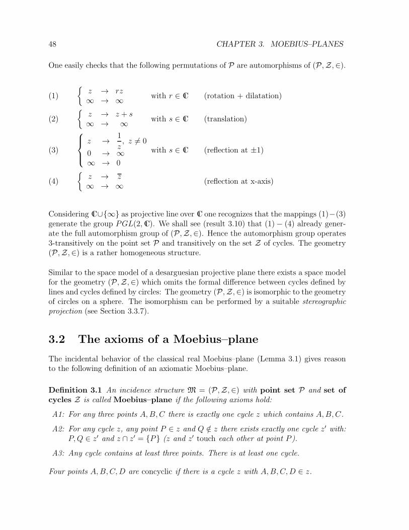
One easily checks that the following permutations of P are automorphisms of (P,Z,∈).
(1)
{
z → rz∞ → ∞
with r ∈ C (rotation + dilatation)
(2)
{
z → z + s∞ → ∞
with s ∈ C (translation)
(3)
z →1
z, z 6= 0
0 → ∞∞ → 0
with s ∈ C (reflection at ±1)
(4)
{
z → z∞ → ∞
(reflection at x-axis)
Considering C∪{∞} as projective line over C one recognizes that the mappings (1)−(3)generate the group PGL(2,C). We shall see (result 3.10) that (1)− (4) already gener-ate the full automorphism group of (P,Z,∈). Hence the automorphism group operates3-transitively on the point set P and transitively on the set Z of cycles. The geometry(P,Z,∈) is a rather homogeneous structure.
Similar to the space model of a desarguesian projective plane there exists a space modelfor the geometry (P,Z,∈) which omits the formal difference between cycles defined bylines and cycles defined by circles: The geometry (P,Z,∈) is isomorphic to the geometryof circles on a sphere. The isomorphism can be performed by a suitable stereographicprojection (see Section 3.3.7).
3.2 The axioms of a Moebius–plane
The incidental behavior of the classical real Moebius–plane (Lemma 3.1) gives reasonto the following definition of an axiomatic Moebius–plane.
Definition 3.1 An incidence structure M = (P,Z,∈) with point set P and set ofcycles Z is called Moebius–plane if the following axioms hold:
A1: For any three points A,B,C there is exactly one cycle z which contains A,B,C.
A2: For any cycle z, any point P ∈ z and Q /∈ z there exists exactly one cycle z′ with:P,Q ∈ z′ and z ∩ z′ = {P} (z and z′ touch each other at point P ).
A3: Any cycle contains at least three points. There is at least one cycle.
Four points A,B,C,D are concyclic if there is a cycle z with A,B,C,D ∈ z.
3.2. THE AXIOMS OF A MOEBIUS–PLANE 49
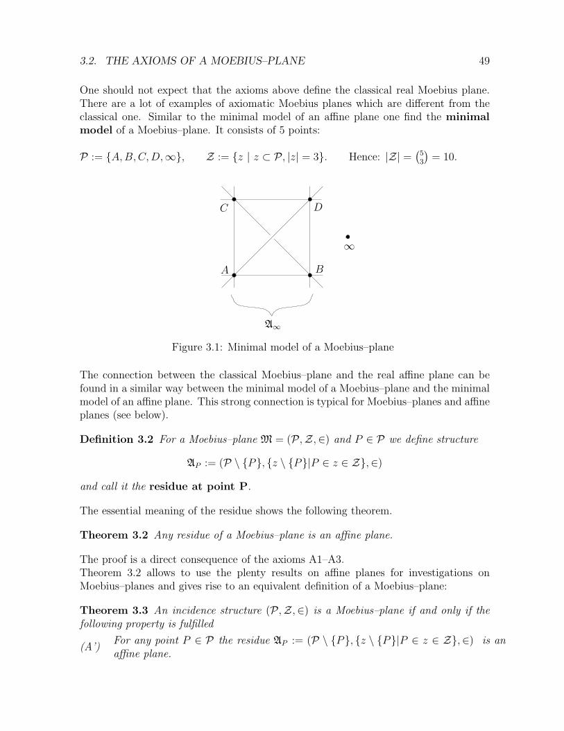
One should not expect that the axioms above define the classical real Moebius plane.There are a lot of examples of axiomatic Moebius planes which are different from theclassical one. Similar to the minimal model of an affine plane one find the minimalmodel of a Moebius–plane. It consists of 5 points:
P := {A,B,C,D,∞}, Z := {z | z ⊂ P, |z| = 3}. Hence: |Z| =(
53
)
= 10.
A B
C D
∞
A∞
Figure 3.1: Minimal model of a Moebius–plane
The connection between the classical Moebius–plane and the real affine plane can befound in a similar way between the minimal model of a Moebius–plane and the minimalmodel of an affine plane. This strong connection is typical for Moebius–planes and affineplanes (see below).
Definition 3.2 For a Moebius–plane M = (P,Z,∈) and P ∈ P we define structure
AP := (P \ {P}, {z \ {P}|P ∈ z ∈ Z},∈)
and call it the residue at point P.
The essential meaning of the residue shows the following theorem.
Theorem 3.2 Any residue of a Moebius–plane is an affine plane.
The proof is a direct consequence of the axioms A1–A3.Theorem 3.2 allows to use the plenty results on affine planes for investigations onMoebius–planes and gives rise to an equivalent definition of a Moebius–plane:
Theorem 3.3 An incidence structure (P,Z,∈) is a Moebius–plane if and only if thefollowing property is fulfilled
(A’)For any point P ∈ P the residue AP := (P \ {P}, {z \ {P}|P ∈ z ∈ Z},∈) is anaffine plane.
50 CHAPTER 3. MOEBIUS–PLANES
For the classical real Moebius–plane any cycle which does not contain point ∞ is anoval conic (circle) in the residue A∞. In general the following is true.
Theorem 3.4 Let be M = (P,Z,∈) a Moebius–plane, AP a residue and z a cycle withP /∈ z. Then: cycle z is an oval in the affine plane AP .
The proof is a direct consequence of axioms A1–A3, too.
For finite Moebius–planes, i.e. |P| <∞, we have (similar to affine planes):
Lemma 3.5 Any two cycles of a Moebius–plane have the same number of points.
This gives reason for the following definition.
Definition 3.3 For a finite Moebius–plane M = (P,Z,∈) and a cycle z ∈ Z the integern := |z| − 1 is called order of M.
From combinatorics we get
Lemma 3.6 Let M = (P,Z,∈) be a Moebius–plane of order n. Thena) any residue AP is an affine plane of order n,b) |P| = n2 + 1, c) |Z| = n(n2 + 1).
3.3 Moebius–planes over a pair of fields
(miquelian Moebius–planes)
3.3.1 The incidence structure M(K, q)
Looking for further examples of Moebius–planes it seems promising to generalize theclassical construction starting with a quadratic form for defining circles in an affinepappian plane. Such Moebius–planes are (as the classical model) characterized by hugehomogeneity and the theorem of MIQUEL. If we generalize the space model of theclassical Moebius–plane (geometry of plane section of a sphere) by replacing the sphereby an ovoid (see Chapter 6 and Section 3.4) in a desarguesian 3-dimensional projectivespace we get an even wider class of Moebius–planes. The relation between the miquelianand ovoidal Moebius–planes can be compared with the relation between pappian anddesarguesian planes.
Let K be a field and q(ξ) := ξ2 + a0ξ + b0, a0, b0 ∈ K an irreducible polynomial overK, i.e. q(k) 6= 0 for all k ∈ K. ρ(x, y) := x2 + a0xy + b0y
2 is the quadratic form withrespect to polynomial q. A(K) is (as hitherto) the affine plane over K with point setK2 and its lines are described by equations y = mx+ b and x = c respectively.
3.3. MIQUELIAN MOEBIUS–PLANES 51
P := K2 ∪ {∞}, ∞ /∈ K, the set of points, and
Z := {g ∪ {∞} | g line of A(K)}
∪ {κ = {(x, y) ∈ K2|ρ(x, y) + cx + dy + e = 0} | |κ| ≥ 2, c, d, e ∈ K} the set ofcycles and
M(K, q) := (P,Z,∈).In order to show that M(K, q) is a Moebius–plane we represent M(K, q) (as in the realcase) over the splitting field E of polynomial q:
There are α1, α2 ∈ E such that q(ξ) = (ξ + α1)(ξ + α2), E is a 2-dimensional vectorspace over K and {1, α1} and {1, α2} are bases of vector space E, i.e. for any elementα ∈ E there are k1, k2, l1, l2 ∈ K such that α = k1 + α1l1 = k2 + α2l2.For the product of two elements α = u+ α1v, ξ = x+ α1y we get:αξ = ux− b0vy + α1(vx+ (u+ a0v)y).(Remember: q(α1) = α2
1 − a0α1 + b0 = 0 !)
Remark 3.1 For the classical real Moebius–plane we have E = C, q(ξ) = ξ2 + 1 andα1 = i, α2 = −i.
We shall recognize that it is essential for the geometry M(K, q) whether α1 = α2 (in-separable case) or α1 6= α2 (separable case). At first we shall discuss the effect onto thesplitting field and the corresponding polynomial:
If q is separable, i.e. α1 6= α2 then the mapping.− : x + α1y → x + α2y = x + ya0 − α1y is an involutorial automorphism of field Eand fromq(ξ) = (ξ + α1)(ξ + α2) = ξ2 + (α1 + α2)ξ + α1α2 = ξ2 + a0ξ + b0 we get:a0 6= 0 if CharK = 2 and 4b20 − a20 6= 0 if CharK 6= 2.
If q is inseparable, i.e. α1 = α2 we get fromq(ξ) = (ξ + α1)(ξ + α2) = ξ2 + 2α1ξ + α2
1 = ξ2 + a0ξ + b0, a0 ∈ K and α1 6= 0 thefollowing statements: a0 = 0, CharK = 2 and b0 is not a square (hence |K| = ∞).
3.3.2 Representation of M(K, q) over E
A point (x, y) ∈ K2 can be represented by ζ := x+α1y ∈ E. Thus K2 can be identifiedby E and we set P = E ∪ {∞}. In case of “q separable” a line can be described byan equation αζ + αζ + c = 0 with α ∈ E \ {0} and c ∈ K and a circle by an equation(ζ − µ)(ζ − µ) = d. (Remember: α2 = a0 − α1, q(−α1) = 0 and ρ(x, y) = ζζ forζ = x + α1y.) In case of “q inseparable” this advantageous description is not possible,but we have a0 = 0 and ρ(x, y) = ζ2.
Conclusion: For the considering below we set:
52 CHAPTER 3. MOEBIUS–PLANES
P = E ∪ {∞} and
if q is separableZ := {{ζ ∈ E | αζ + αζ + c = 0} ∪ {∞} | 0 6= α ∈ E, c ∈ K}
∪ {κ = {ζ ∈ E | (ζ − µ)(ζ − µ) = d} | µ ∈ E, d ∈ K, |κ| ≥ 2}
if q is inseparableZ := {{x+ α1y ∈ E | ax+ by + c = 0} ∪ {∞} | a, b, c ∈ K, (a, b) 6= (0, 0)}
∪ {κ = {x+ α1y ∈ E | x2 + b0y2 + cx+ dy + e = 0} | c, d, e ∈ K, |κ| ≥ 2}
3.3.3 Automorphisms of M(K, q), M(K, q) is Moebius–plane
The advantage describing M(K, q) over E is the simple representation of its automor-phisms.
Lemma 3.7 The following mappings of P are automorphisms of M(K, q).
(1) :
{
ζ → δζ, 0 6= δ ∈ E∞ → ∞
, (2) :
{
ζ → ζ + τ, τ ∈ E∞ → ∞
,
(3) :
ζ →1
ζ, ζ 6= 0
0 → ∞∞ → 0
, case “q separable”: (4) :
{
ζ → ζ∞ → ∞ .
Proof: a) Let q be separable. In this case the mappings (1), (2) and (4) are obviouslyautomorphisms. Mapping (3) sends the line αζ+αζ+c = 0 onto curve αζ+αζ+cζζ = 0which is a line (if c = 0) or a circle (if c 6= 0). A circle (ζ−µ)(ζ − µ) = d is sent to curve1− µζ − µζ = (d− µµ)ζζ which is a line (if d = µµ) or a circle (if d 6= µµ). Because aline αζ + αζ + c = 0 or a circle (ζ − µ)(ζ − µ) = d contains point (0, 0) if and only ifc = 0 or d = µµ respectively we get: (3) is an automorphism, too.b) Now let q be inseparable. In this case we have CharK = 2, a0 = 0 and α1 = α2 andfor δ = u + α1v and ζ = x + α1y we get δζ = ux + b0vy + α1(vx + uy). One checkseasily that ζ → δζ sends lines onto lines and circles onto circles. Obviously mapping(2) is an automorphism, too. For the proof that (3) is an automorphism one uses forζ = y + α1y 6= 0 the relation1
ζ=
ζ
ζ2=
x
x2 + b0y2+ α1
y
x2 + b0y2. 2
With the aid of automorphisms (1), (2), (3) one assures oneself of the validity of thefollowing theorem.
Theorem 3.8 The group PGL(2, E) of fractional linear mappings (Moebius transfor-mations)
ζ →αζ + β
γζ + δ, αδ − βγ 6= 0
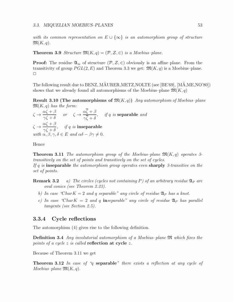
3.3. MIQUELIAN MOEBIUS–PLANES 53
with its common representation on E ∪ {∞} is an automorphism group of structureM(K, q).
Theorem 3.9 Structure M(K, q) = (P,Z,∈) is a Moebius–plane.
Proof: The residue A∞ of structure (P,Z,∈) obviously is an affine plane. From thetransitivity of group PGL(2, E) and Theorem 3.3 we get: M(K, q) is a Moebius–plane.2
The following result due to BENZ, MAURER,METZ,NOLTE (see [BE’69], [MA,ME,NO’80])shows that we already found all automorphisms of the Moebius–plane M(K, q)
Result 3.10 (The automorphisms of M(K, q)) Any automorphism of Moebius–planeM(K, q) has the form:
ζ →αζ + β
γζ + δor ζ →
αζ + β
γζ + δ, if q is separable and
ζ →αζ + β
γζ + δ, if q is inseparable
with α, β, γ, δ ∈ E and αδ − βγ 6= 0.
Hence
Theorem 3.11 The automorphism group of the Moebius–plane M(K, q) operates 3-transitively on the set of points and transitively on the set of cycles.If q is inseparable the automorphism group operates even sharply 3-transitive on theset of points.
Remark 3.2 a) The circles (cycles not containing P ) of an arbitrary residue AP areoval conics (see Theorem 2.23).
b) In case “CharK = 2 and q separable” any circle of residue AP has a knot.
c) In case “CharK = 2 and q inseparable” any circle of residue AP has paralleltangents (see Section 2.5).
3.3.4 Cycle reflections
The automorphism (4) gives rise to the following definition.
Definition 3.4 Any involutorial automorphism of a Moebius–plane M which fixes thepoints of a cycle z is called reflection at cycle z.
Because of Theorem 3.11 we get
Theorem 3.12 In case of “q separable” there exists a reflection at any cycle ofMoebius–plane M(K, q).
54 CHAPTER 3. MOEBIUS–PLANES
Throughout the following considerations we always assume “q is separable”. Hencereflections at cycles exist.In order to find some properties typical for cycle reflections in M(K, q) we discuss thereflection σ at cycle y = 0. It induces in residue A∞ = A(K) the reflection σ : (x, y) →(x+a0y,−y) at the x-axis with center in direction (a0,−2). A circle (ζ−ζ0)(ζ − ζ0) = kwill be send onto itself if and only if ζ0 ∈ K (proof as in real case). Herewith we findthat for any two points ζ1, ζ2 ∈ E \K with ζ1 6= ζ2 there is exactly one cycle fixed by σcontaining ζ1, ζ2:in case of ζ1 − ζ2 ∈ K · (a0 − 2α1) the fixed cycle is K · (a0 − 2α1) ∪ {∞},in case of ζ1 − ζ2 /∈ K · (a0 − 2α1) the fixed cycle is (ζ − ζ0)(ζ − ζ0) = k with ζ0 ∈ K.From the transitivity of the automorphism group of M(K, q) (see Theorem 3.11) we get
Lemma 3.13 Let be q separable, σ a cycle reflection of M(K, q) and A,B two points.Then A,B, σ(A), σ(B) lie on a common cycle.
The importance of this statement shows the following result due to KARZEL,MAURER([KA,MA’82]).
Result 3.14 A Moebius–plane M is isomorphic to a Moebius–plane M(K, q) with sep-arable q if and only if the following holds:(CR) For any cycle z there is a reflection at z.
(AB)For any cycle reflection σ and any two points A,B the four points A,B, σ(A), σ(B)lie on a cycle. (σ is called inversion.)
(For finite Moebius–planes property (CR) is sufficient (see [DE’68], p.277).
The following considerations show a further essential property of cycle reflections of aMoebius–plane M(K, q):Conjugation of reflection ζ → ζ (at cycle K ∪ {∞}) by mapping ζ → δζ, δ ∈ E \ {0}we get the reflection ζ → δ
δζ at cycle Kδ ∪ {∞}. One easily checks that the product of
three of such reflections at cycles containing 0 and ∞ represent a fourth reflection at acycle containing 0 and ∞. Because of Theorem 3.11 we get
Lemma 3.15 (Theorem of 3 reflections) For a Moebius–plane M(K, q), q separa-ble, the following statement holds:For any three cycles z1, z2, z3 through points A 6= B the product of the reflections atz1, z2, z3 is a reflection at a cycle z4 through A,B.
Property (AB) of Result 3.14 can be replaced with property (3R) (Theorem of 3 reflec-tions) (see LANG [LA’81]).
Result 3.16 A Moebius–plane M is isomorphic to a Moebius–plane M(K, q) with qseparable if(CR) For any cycle z there is a reflection at z.
(3R)For any three cycles z1, z2, z3 through arbitrary points A 6= B the product ofthe reflections at z1, z2, z3 is a reflection at a cycle z4 through A,B.
3.3. MIQUELIAN MOEBIUS–PLANES 55
3.3.5 Angles in affine plane A(K, q)
Let be A(K, q) the description of affine plane A(K) over the splitting field E of poly-nomial q. With the aid of the multiplication of E we define a measure for angles inA(K, q).
Definition 3.5 Let be g1, g2 be lines of an affine plane. The ordered pair [g1, g2] iscalled angle.
In order to get a theorem for A(K, q) similar to the inscribed angle theorem of the realplane we introduce a suitable measure for angles.
Definition 3.6 For 0 6= ζ ∈ E let be < ζ > the line containing 0 and ζ (in A(K, q)).On set G0 := {< ζ > | 0 6= ζ ∈ E} we define summation +:For 0 6= ζ1, ζ2 ∈ E we set < ζ1 > + < ζ2 >:=< ζ1ζ2 >.
Obviously
Lemma 3.17 (G0,+) is a commutative group, K =< 1 > is the neutral element andfor < ζ >∈ G0 and “q separable” < ζ > is the inverse element. In case of “qinseparable” any element 6= id is involutorial.(G0,+) is isomorphic to (E∗/K∗, ·) with E∗ := E \ {0}, K∗ := K \ {0}.
Definition 3.7 Let be g1, g2 lines of A(K, q), ζ1, ζ′1 ∈ g1 with ζ1 6= ζ ′1 and ζ2, ζ
′2 ∈ g2
with ζ1 6= ζ ′1 then
∠(g1, g2) :=< ζ1 − ζ ′1 > − < ζ2 − ζ ′2 >=<ζ1−ζ′
1
ζ2−ζ′2
>
is the measure of angle [g1, g2].
Remark 3.3 In [BE’73] BENZ introduces a measure for angles between pairs of cyclesusing the cross ratio on the projective line E ∪ {∞}.
For the measurement of angles of triangles we give a further definition:
Definition 3.8 For any three points ζ1, ζ2, ζ3 ∈ E we set
∠(ζ1, ζ2, ζ3) :=< ζ1 − ζ2 > − < ζ3 − ζ2 >=<ζ1 − ζ2ζ3 − ζ2
>.
For the sum of the angles of a triangle we get
Lemma 3.18 For any three points ζ1, ζ2, ζ3 ∈ E we have
∠(ζ1, ζ2, ζ3) + ∠(ζ2, ζ3, ζ1) + ∠(ζ3, ζ1, ζ2) = 0.
Comparing the last statement with the well known one in the real case one has to takeinto account that the measure for angles defined above matches the real one modulo180◦.Now we shall prove a theorem analogous to the “inscribed angle theorem” which givesus a tool to characterize 4 points on a circle in A(K, q).
56 CHAPTER 3. MOEBIUS–PLANES
Definition 3.9 A point set of A(K, q) which fulfills an equation of the form
x2 + a0xy + b0y2 + cx+ dy + e = 0
and contains at least two points is called circle of A(K, q).
Theorem 3.19 (4 points on a circle) Four points ζ1, ζ2, ζ3, ζ4 ∈ E lie on a circle ofA(K, q) if no three are collinear and if ∠(ζ1, ζ3, ζ2) = ∠(ζ1, ζ4, ζ2)
Proof: We shall show that the condition ∠(ζ1, ζ3, ζ2) = ∠(ζ1, ζ4, ζ2) for points ζi =xi + α1yi, i = 1, 2, 3, 4 is equivalent to the fact that their coordinates xi, yi satisfy anequation x2 + a0xy + b0y
2 + cx+ dy + e = 0.For the points ζ1, ζ2, ζ3, ζ4, no three collinear, we suppose ∠(ζ1, ζ3, ζ2) = ∠(ζ1, ζ, ζ2), i.e.< ζ1−ζ3
ζ2−ζ3>=< ζ1−ζ
ζ2−ζ>. In order to cover both cases “q separable” and “q insepara-
ble” we declare the mapping · as identity if q is inseparable. Hence < ζ1−ζ3ζ2−ζ3
>=<
(ζ1 − ζ)(ζ2 − ζ) > because of Lemma 3.17. For ζi = xi + α1yi, α1α2 = b0, α1 + α2 = a0and the abbreviations xik := xi − xk and yik := yi − yk we get (ζ1 − ζ3)(ζ2 − ζ3) =x13x23 + a0x13y23 + b0y13y23 +α1(y13x23 − y23x13). Because ζ1, ζ2, ζ3 are not collinear wehave y13x23 − y23x13 6= 0. The analogous consideration for (ζ1 − ζ)(ζ2 − ζ) yields:
x13x23 + a0x13y23 + b0y13y23y13x23 − y23x13
=(x1 − x)(x2 − x) + a0(x1 − x(y2 − y) + b0(y1 − y)(y2 − y)
(y1 − y)(x2 − x)− (y2 − y)(x1 − x)
which is the “3-point-form” of the circle through ζ1, ζ2, ζ3 and hence equivalent to anequation of the form x2 + a0xy+ b0y
2 + cx+ dy+ e = 0 and the coordinates of ζ1, ζ2, ζ3fulfill this equation.Hence the equation ∠(ζ1, ζ3, ζ2) = ∠(ζ1, ζ4, ζ2) is equivalent to the fact that ζ lies on thecircle determined by ζ1, ζ2, ζ3.(For the classical real case the left hand side of the 3-point-form is the cotangens of theangle at P3.) 2
3.3.6 Theorem of MIQUEL in M(K, q)
With the aid of Theorem 3.19 we shall proof the Theorem of MIQUEL and a degener-ation of it in the Moebius–plane M(K, q).
Theorem 3.20 (Theorem of MIQUEL) For the Moebius–plane M(K, q) the follow-ing is true:If for any 8 points P1, ..., P8 which can be assigned to the vertices of a cube such that thepoints in 5 faces correspond to concyclical quadruples than the sixth quadruple of pointsis concyclical, too.
Proof: Because of the transitivity of the automorphism group of M(K, q) we shallconfine on the case P8 = ∞. We use for P the representation over the splitting field Eof polynomial q. Hence Pi ∈ E for i = 1, ..., 7. With the abbreviation mik =< Pi−Pk >(see Section 3.3.5) we get from Theorem 3.17 (see Fig. 3.3):
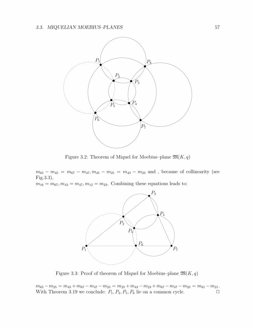
3.3. MIQUELIAN MOEBIUS–PLANES 57
P1
P2
P3
P4P5
P6
P7
P8
Figure 3.2: Theorem of Miquel for Moebius–plane M(K, q)
m65 − m45 = m67 − m47, m45 − m25 = m43 − m23 and , because of collinearity (seeFig.3.3),m16 = m67, m43 = m47, m12 = m23. Combining these equations leads to:
P1
P2
P3
P4
P5
P6
P7
Figure 3.3: Proof of theorem of Miquel for Moebius–plane M(K, q)
m65−m25 = m45+m67−m47−m25 = m25+m43−m23+m67−m47−m25 = m61−m21.With Theorem 3.19 we conclude: P1, P2, P5, P6 lie on a common cycle. 2
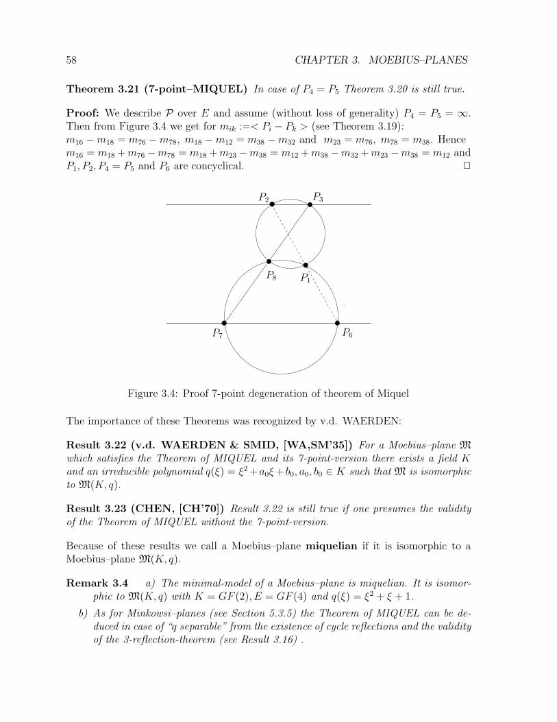
58 CHAPTER 3. MOEBIUS–PLANES
Theorem 3.21 (7-point–MIQUEL) In case of P4 = P5 Theorem 3.20 is still true.
Proof: We describe P over E and assume (without loss of generality) P4 = P5 = ∞.Then from Figure 3.4 we get for mik :=< Pi − Pk > (see Theorem 3.19):m16 −m18 = m76 −m78, m18 −m12 = m38 −m32 and m23 = m76, m78 = m38. Hencem16 = m18 +m76 −m78 = m18 +m23 −m38 = m12 +m38 −m32 +m23 −m38 = m12 andP1, P2, P4 = P5 and P6 are concyclical. 2
P1
P2 P3
P6P7
P8
Figure 3.4: Proof 7-point degeneration of theorem of Miquel
The importance of these Theorems was recognized by v.d. WAERDEN:
Result 3.22 (v.d. WAERDEN & SMID, [WA,SM’35]) For a Moebius–plane M
which satisfies the Theorem of MIQUEL and its 7-point-version there exists a field Kand an irreducible polynomial q(ξ) = ξ2+a0ξ+ b0, a0, b0 ∈ K such that M is isomorphicto M(K, q).
Result 3.23 (CHEN, [CH’70]) Result 3.22 is still true if one presumes the validityof the Theorem of MIQUEL without the 7-point-version.
Because of these results we call a Moebius–plane miquelian if it is isomorphic to aMoebius–plane M(K, q).
Remark 3.4 a) The minimal-model of a Moebius–plane is miquelian. It is isomor-phic to M(K, q) with K = GF (2), E = GF (4) and q(ξ) = ξ2 + ξ + 1.
b) As for Minkowsi–planes (see Section 5.3.5) the Theorem of MIQUEL can be de-duced in case of “q separable” from the existence of cycle reflections and the validityof the 3-reflection-theorem (see Result 3.16) .
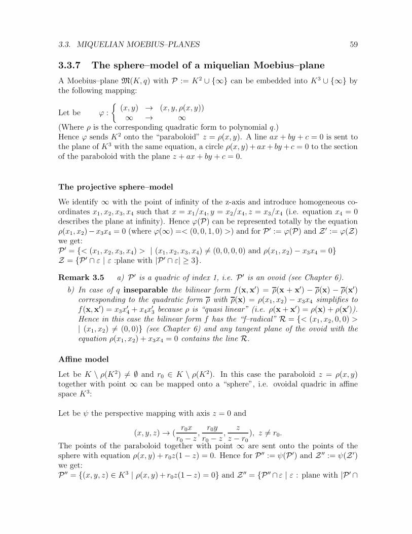
3.3. MIQUELIAN MOEBIUS–PLANES 59
3.3.7 The sphere–model of a miquelian Moebius–plane
A Moebius–plane M(K, q) with P := K2 ∪ {∞} can be embedded into K3 ∪ {∞} bythe following mapping:
Let be ϕ :
{
(x, y) → (x, y, ρ(x, y))∞ → ∞
(Where ρ is the corresponding quadratic form to polynomial q.)Hence ϕ sends K2 onto the “paraboloid” z = ρ(x, y). A line ax + by + c = 0 is sent tothe plane of K3 with the same equation, a circle ρ(x, y)+ ax+ by+ c = 0 to the sectionof the paraboloid with the plane z + ax+ by + c = 0.
The projective sphere–model
We identify ∞ with the point of infinity of the z-axis and introduce homogeneous co-ordinates x1, x2, x3, x4 such that x = x1/x4, y = x2/x4, z = x3/x4 (i.e. equation x4 = 0describes the plane at infinity). Hence ϕ(P) can be represented totally by the equationρ(x1, x2)−x3x4 = 0 (where ϕ(∞) =< (0, 0, 1, 0) >) and for P ′ := ϕ(P) and Z ′ := ϕ(Z)we get:P ′ = {< (x1, x2, x3, x4) > | (x1, x2, x3, x4) 6= (0, 0, 0, 0) and ρ(x1, x2)− x3x4 = 0}Z = {P ′ ∩ ε | ε :plane with |P ′ ∩ ε| ≥ 3}.
Remark 3.5 a) P ′ is a quadric of index 1, i.e. P ′ is an ovoid (see Chapter 6).
b) In case of q inseparable the bilinear form f(x,x′) = ρ(x + x′) − ρ(x) − ρ(x′)corresponding to the quadratic form ρ with ρ(x) = ρ(x1, x2) − x3x4 simplifies tof(x,x′) = x3x
′4 + x4x
′3 because ρ is “quasi linear” (i.e. ρ(x+ x′) = ρ(x) + ρ(x′)).
Hence in this case the bilinear form f has the “f–radical” R = {< (x1, x2, 0, 0) >| (x1, x2) 6= (0, 0)} (see Chapter 6) and any tangent plane of the ovoid with theequation ρ(x1, x2) + x3x4 = 0 contains the line R.
Affine model
Let be K \ ρ(K2) 6= ∅ and r0 ∈ K \ ρ(K2). In this case the paraboloid z = ρ(x, y)together with point ∞ can be mapped onto a “sphere”, i.e. ovoidal quadric in affinespace K3:
Let be ψ the perspective mapping with axis z = 0 and
(x, y, z) → (r0x
r0 − z,r0y
r0 − z,
z
z − r0), z 6= r0.
The points of the paraboloid together with point ∞ are sent onto the points of thesphere with equation ρ(x, y) + r0z(1− z) = 0. Hence for P ′′ := ψ(P ′) and Z ′′ := ψ(Z ′)we get:P ′′ = {(x, y, z) ∈ K3 | ρ(x, y)+ r0z(1− z) = 0} and Z ′′ = {P ′′∩ ε | ε : plane with |P ′ ∩
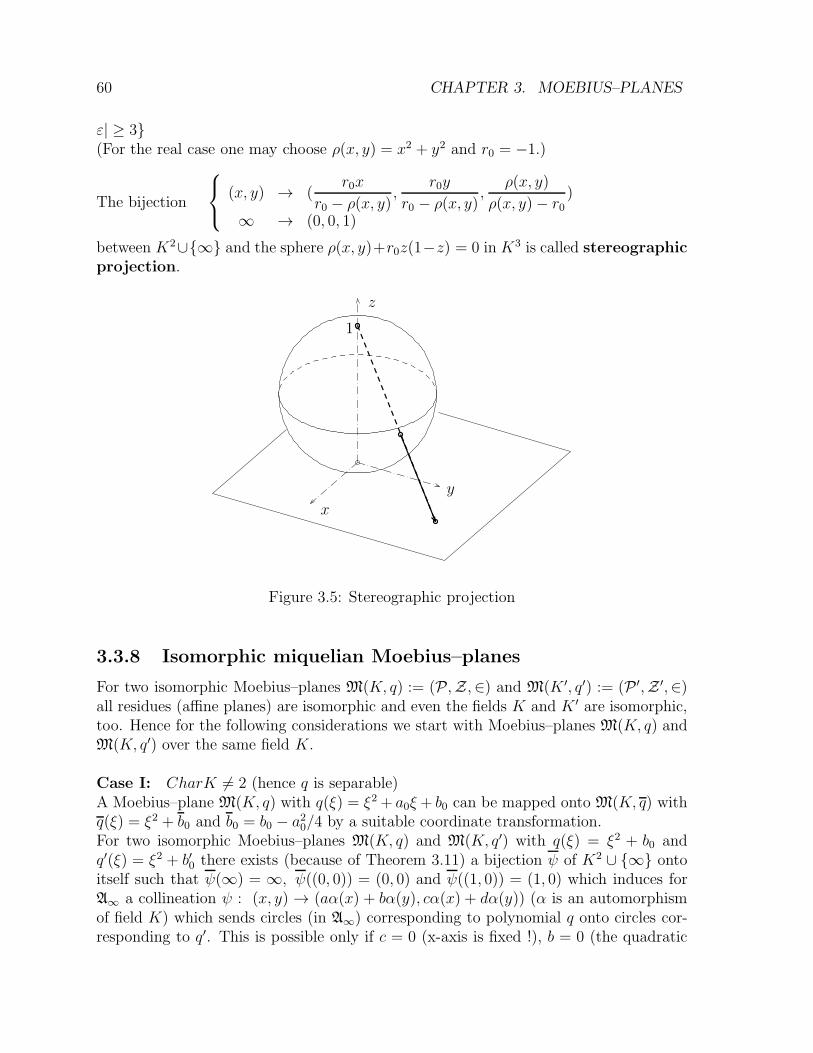
60 CHAPTER 3. MOEBIUS–PLANES
ε| ≥ 3}(For the real case one may choose ρ(x, y) = x2 + y2 and r0 = −1.)
The bijection
(x, y) → (r0x
r0 − ρ(x, y),
r0y
r0 − ρ(x, y),
ρ(x, y)
ρ(x, y)− r0)
∞ → (0, 0, 1)
between K2∪{∞} and the sphere ρ(x, y)+r0z(1−z) = 0 in K3 is called stereographicprojection.
x
y
z
1
Figure 3.5: Stereographic projection
3.3.8 Isomorphic miquelian Moebius–planes
For two isomorphic Moebius–planes M(K, q) := (P,Z,∈) and M(K ′, q′) := (P ′,Z ′,∈)all residues (affine planes) are isomorphic and even the fields K and K ′ are isomorphic,too. Hence for the following considerations we start with Moebius–planes M(K, q) andM(K, q′) over the same field K.
Case I: CharK 6= 2 (hence q is separable)A Moebius–plane M(K, q) with q(ξ) = ξ2 + a0ξ+ b0 can be mapped onto M(K, q) withq(ξ) = ξ2 + b0 and b0 = b0 − a20/4 by a suitable coordinate transformation.For two isomorphic Moebius–planes M(K, q) and M(K, q′) with q(ξ) = ξ2 + b0 andq′(ξ) = ξ2 + b′0 there exists (because of Theorem 3.11) a bijection ψ of K2 ∪ {∞} ontoitself such that ψ(∞) = ∞, ψ((0, 0)) = (0, 0) and ψ((1, 0)) = (1, 0) which induces forA∞ a collineation ψ : (x, y) → (aα(x) + bα(y), cα(x) + dα(y)) (α is an automorphismof field K) which sends circles (in A∞) corresponding to polynomial q onto circles cor-responding to q′. This is possible only if c = 0 (x-axis is fixed !), b = 0 (the quadratic
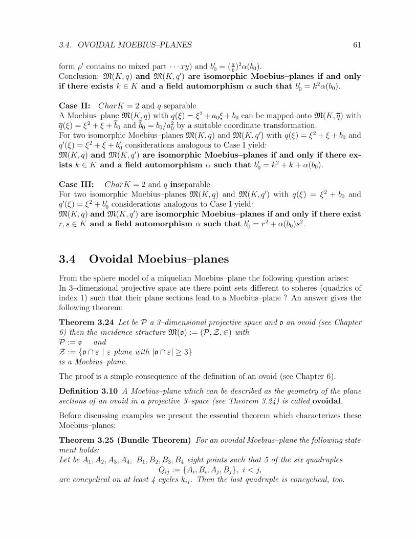
3.4. OVOIDAL MOEBIUS–PLANES 61
form ρ′ contains no mixed part · · ·xy) and b′0 = (ab)2α(b0).
Conclusion: M(K, q) and M(K, q′) are isomorphic Moebius–planes if and onlyif there exists k ∈ K and a field automorphism α such that b′0 = k2α(b0).
Case II: CharK = 2 and q separableA Moebius–plane M(K, q) with q(ξ) = ξ2+ a0ξ+ b0 can be mapped onto M(K, q) withq(ξ) = ξ2 + ξ + b0 and b0 = b0/a
20 by a suitable coordinate transformation.
For two isomorphic Moebius–planes M(K, q) and M(K, q′) with q(ξ) = ξ2 + ξ + b0 andq′(ξ) = ξ2 + ξ + b′0 considerations analogous to Case I yield:M(K, q) and M(K, q′) are isomorphic Moebius–planes if and only if there ex-ists k ∈ K and a field automorphism α such that b′0 = k2 + k + α(b0).
Case III: CharK = 2 and q inseparableFor two isomorphic Moebius–planes M(K, q) and M(K, q′) with q(ξ) = ξ2 + b0 andq′(ξ) = ξ2 + b′0 considerations analogous to Case I yield:M(K, q) and M(K, q′) are isomorphic Moebius–planes if and only if there existr, s ∈ K and a field automorphism α such that b′0 = r2 + α(b0)s
2.
3.4 Ovoidal Moebius–planes
From the sphere model of a miquelian Moebius–plane the following question arises:In 3–dimensional projective space are there point sets different to spheres (quadrics ofindex 1) such that their plane sections lead to a Moebius–plane ? An answer gives thefollowing theorem:
Theorem 3.24 Let be P a 3–dimensional projective space and o an ovoid (see Chapter6) then the incidence structure M(o) := (P,Z,∈) withP := o andZ := {o ∩ ε | ε plane with |o ∩ ε| ≥ 3}is a Moebius–plane.
The proof is a simple consequence of the definition of an ovoid (see Chapter 6).
Definition 3.10 A Moebius–plane which can be described as the geometry of the planesections of an ovoid in a projective 3–space (see Theorem 3.24) is called ovoidal.
Before discussing examples we present the essential theorem which characterizes theseMoebius–planes:
Theorem 3.25 (Bundle Theorem) For an ovoidal Moebius–plane the following state-ment holds:Let be A1, A2, A3, A4, B1, B2, B3, B4 eight points such that 5 of the six quadruples
Qij := {Ai, Bi, Aj , Bj}, i < j,are concyclical on at least 4 cycles kij. Then the last quadruple is concyclical, too.
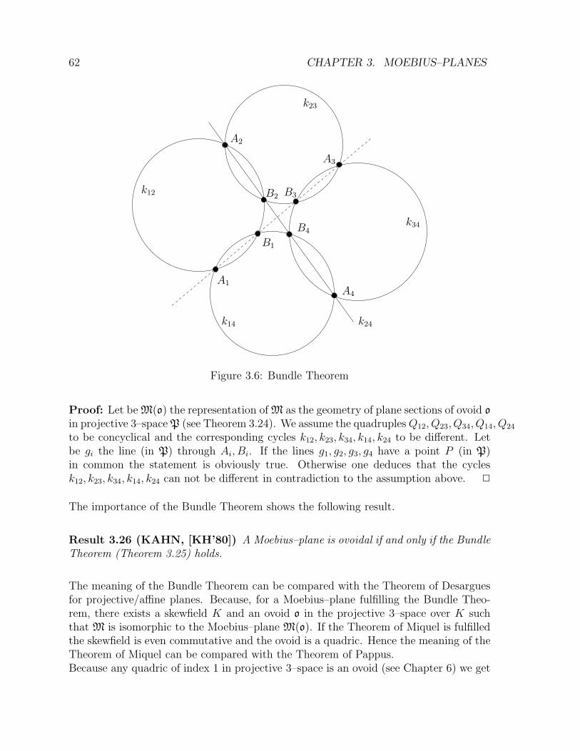
62 CHAPTER 3. MOEBIUS–PLANES
A1
A2
A3
A4
B1
B2 B3
B4
k12
k14
k34
k23
k24
Figure 3.6: Bundle Theorem
Proof: Let beM(o) the representation ofM as the geometry of plane sections of ovoid o
in projective 3–spaceP (see Theorem 3.24). We assume the quadruplesQ12, Q23, Q34, Q14, Q24
to be concyclical and the corresponding cycles k12, k23, k34, k14, k24 to be different. Letbe gi the line (in P) through Ai, Bi. If the lines g1, g2, g3, g4 have a point P (in P)in common the statement is obviously true. Otherwise one deduces that the cyclesk12, k23, k34, k14, k24 can not be different in contradiction to the assumption above. 2
The importance of the Bundle Theorem shows the following result.
Result 3.26 (KAHN, [KH’80]) A Moebius–plane is ovoidal if and only if the BundleTheorem (Theorem 3.25) holds.
The meaning of the Bundle Theorem can be compared with the Theorem of Desarguesfor projective/affine planes. Because, for a Moebius–plane fulfilling the Bundle Theo-rem, there exists a skewfield K and an ovoid o in the projective 3–space over K suchthat M is isomorphic to the Moebius–plane M(o). If the Theorem of Miquel is fulfilledthe skewfield is even commutative and the ovoid is a quadric. Hence the meaning of theTheorem of Miquel can be compared with the Theorem of Pappus.Because any quadric of index 1 in projective 3–space is an ovoid (see Chapter 6) we get
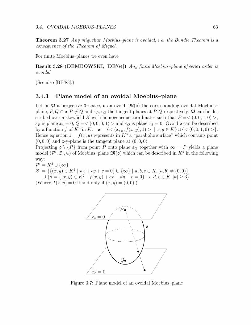
3.4. OVOIDAL MOEBIUS–PLANES 63
Theorem 3.27 Any miquelian Moebius–plane is ovoidal, i.e. the Bundle Theorem is aconsequence of the Theorem of Miquel.
For finite Moebius–planes we even have
Result 3.28 (DEMBOWSKI, [DE’64]) Any finite Moebius–plane of even order isovoidal.
(See also [BP’83].)
3.4.1 Plane model of an ovoidal Moebius–plane
Let be P a projective 3–space, o an ovoid, M(o) the corresponding ovoidal Moebius–plane, P,Q ∈ o, P 6= Q and εP , εQ the tangent planes at P,Q respectively. P can be de-scribed over a skewfield K with homogeneous coordinates such that P =< (0, 0, 1, 0) >,εP is plane x4 = 0, Q =< (0, 0, 0, 1) > and εQ is plane x3 = 0. Ovoid o can be describedby a function f of K2 in K: o = {< (x, y, f(x, y), 1) > | x, y ∈ K}∪{< (0, 0, 1, 0) >}.Hence equation z = f(x, y) represents in K3 a “parabolic surface” which contains point(0, 0, 0) and x-y-plane is the tangent plane at (0, 0, 0).Projecting o \ {P} from point P onto plane εQ together with ∞ = P yields a planemodel (P ′,Z ′,∈) of Moebius–plane M(o) which can be described in K2 in the followingway:P ′ = K2 ∪ {∞}Z ′ = {{(x, y) ∈ K2 | ax+ by + c = 0} ∪ {∞} | a, b, c ∈ K, (a, b) 6= (0, 0)}
∪ {κ = {(x, y) ∈ K2 | f(x, y) + cx+ dy + e = 0} | c, d, e ∈ K, |κ| ≥ 3}(Where f(x, y) = 0 if and only if (x, y) = (0, 0).)
P
Q
o
x3 = 0
x4 = 0
Figure 3.7: Plane model of an ovoidal Moebius–plane
64 CHAPTER 3. MOEBIUS–PLANES
Remark 3.6 Examples for suitable functions f (especially for the real case) are con-tained in Section 6.3.
3.4.2 Examples of ovoidal Moebius–planes
It suffice to give ovoids in a projective 3–space. In the real case there are a lot ofpossibilities to construct ovoids which are no quadrics (see Chapter 6). For the finitecase we get from the Theorem of SEGRE (2.27): Any ovoid in a projective 3–space ofodd order is already a quadric (see Chapter 6). Hence:
Theorem 3.29 Any finite ovoidal Moebius–plane of odd order is miquelian.
The Moebius–planes of even order known until now are either miquelian or ovoidal overa TITS-SUZUKI–ovoid (see Chapter 6). Such an ovoid exists for any field GF (2n) with“n odd”:
Using the mapping σ : x → x(2n+12 ) the cycles of the plane model (of the Moebius–
plane) which do not contain point ∞ can be described by an equation xσx2+xy+ yσ +ax+ by + c = 0.In case of “n = 1” only we get a miquelian Moebius–plane (minimal model).
One gets further examples of non miquelian ovoidal Moebius–planes with good alge-braic representations if one uses the Moufang–ovoids of TITS (see [TI’62]) which existfor certain infinite fields of characteristic 2.
Finally it should be mentioned that for any infinite projective 3–space there exist ovoidswhich are constructed by transfinite induction (see [HE’71], p. 210). Hence the class ofovoidal Moebius–planes is rather rich.
3.5 Non ovoidal Moebius–planes
All examples of non ovoidal Moebius–planes are due to EWALD (see [EW’67]). We giveone class of such examples:
Let be k a strongly convex, differentiable, closed curve of the real affine plane A(IR) and∆+ the group of dilatations with a positive scalefactor: (x, y) → (ax+ s, ay+ t), a > 0andP := IR
2 ∪ {∞}, ∞ /∈ IR,Z := {{δ(k) | δ ∈ ∆+} ∪ {g ∪ {∞} | g line of A(IR)}.Then: (P,Z,∈) is a Moebius–plane.(See also [GR’74c].)
3.6. FINAL REMARK 65
3.6 Final remark
Further results on Moebius–planes can be found in the books of BENZ [BE’73] andDEMBOWSKI [DE’68].
66 CHAPTER 3. MOEBIUS–PLANES
Chapter 4
LAGUERRE–PLANES
Literature: [BE’73]
4.1 The classical real Laguerre–plane
Originally the classical Laguerre–plane was defined as the geometry of the oriented linesand circles in the real euclidean plane (see BENZ [BE’73]). Here we prefer the parabolamodel considering the Moebius–plane as the geometry of the circles, the Laguerre–planethe geometry of parabolas and the Minkowski–plane the geometry of hyperbolas in thereal plane.
Let be A(IR) the real affine plane with its common coordinatization. In order to ho-mogenize the geometry of the parabolas y = ax2 + bx + c, a, b, c ∈ IR (in case of a 6= 0parabolas, in case of a = 0 lines) it is convenient to introduce the curvature factors asadditional points. We get basic properties for incidence similar to the Moebius–plane.
We define:P := (IR ∪ {∞})× IR = IR
2 ∪ ({∞} × IR), ∞ /∈ IR, the set of points,Z := {{(x, y) ∈ IR
2 | y = ax2 + bx+ c} ∪ {(∞, a)} | a, b, c ∈ IR} the set of cycles.The incidence structure (P,Z,∈) is called classical real Laguerre–plane.
Unlike to Moebius–planes there exist pairs of points which cannot be connected by cy-cles. Hence we define: Two points A,B are parallel (A ‖ B) if A = B or there isno cycle containing A and B. For the description of the classical real Laguerre–planeabove two points (a1, a2), (b1, b2) are parallel if and only if a1 = b1. Obviously ‖ is anequivalence relation.
The incidence structure (P,Z,∈) has the following properties:
67
68 CHAPTER 4. LAGUERRE–PLANES
Lemma 4.1 a) For any three points A,B,C, pairwise not parallel, there is exactly onecycle z containing A,B,C.b) For any point P and any cycle z there is exactly one point P ′ ∈ z such that P ‖ P ′.c) For any cycle z, any point P ∈ z and any point Q /∈ z which is not parallel to Pthere is exactly one cycle z′ through P,Q with z ∩ z′ = {P}, i.e. “z and z′ touch eachother at P”.
Proof: a) and b) are obvious. The validity of c) is recognized easily if one uses thetransitivity of the automorphism group of (P,Z,∈) and by setting P = (∞, 0). Nowc) is equivalent to the parallel axiom of the affine plane A(IR). The transitivity is aconsequence of the fact that the translations (x, y) → (x + s, y + t) and the mapping(x, y) → ( 1
x, yx2 ), x 6= 0 can be extended to automorphisms of (P,Z,∈) (see Section
4.3.2). 2
Similar to the sphere model of the classical real Moebius–plane there is a space model forthe classical Laguerre–plane: (P,Z,∈) is isomorphic to the geometry of plane sectionsof a circular cylinder in IR
3 (see Section 4.4).
4.2 The axioms of a Laguerre–plane
Lemma 4.1 gives rise to the following definition:
Definition 4.1 Let L = (P,Z,∈) be an incidence structure with point set P and setof cycles Z. Two points A,B are parallel (A ‖ B) if A = B or there is no cyclecontaining A and B. L is called Laguerre–plane if the following axioms hold:
B1: For any three points A,B,C, pairwise not parallel, there is exactly one cycle zwhich contains A,B,C.
B2: For any point P and any cycle z there is exactly one point P ′ ∈ z such that P ‖ P ′.
B3: For any cycle z, any point P ∈ z and any point Q /∈ z which is not parallel to Pthere is exactly one cycle z′ through P,Q with z ∩ z′ = {P}, i.e. “z and z′ toucheach other at P”.
B4: Any cycle contains at least three points, there is at least one cycle. There are atleast four points not on a cycle.
Four points A,B,C,D are concyclic if there is a cycle z with A,B,C,D ∈ z.
From the definition of relation ‖ and axiom B2 we get
Lemma 4.2 Relation ‖ is an equivalence relation.
Following the cylinder model of the classical Laguerre-plane we introduce the denotation:
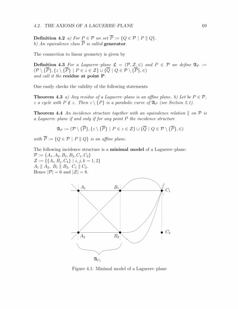
4.2. THE AXIOMS OF A LAGUERRE–PLANE 69
Definition 4.2 a) For P ∈ P we set P := {Q ∈ P | P ‖ Q}.b) An equivalence class P is called generator.
The connection to linear geometry is given by
Definition 4.3 For a Laguerre–plane L = (P,Z,∈) and P ∈ P we define AP :=(P \ {P}, {z \ {P} | P ∈ z ∈ Z} ∪ {Q | Q ∈ P \ {P},∈)and call it the residue at point P.
One easily checks the validity of the following statements
Theorem 4.3 a) Any residue of a Laguerre–plane is an affine plane. b) Let be P ∈ P,z a cycle with P /∈ z. Then z \ {P} is a parabolic curve of AP (see Section 2.1).
Theorem 4.4 An incidence structure together with an equivalence relation ‖ on P isa Laguerre–plane if and only if for any point P the incidence structure
AP := (P \ {P}, {z \ {P} | P ∈ z ∈ Z} ∪ {Q | Q ∈ P \ {P},∈)
with P := {Q ∈ P | P ‖ Q} is an affine plane.
The following incidence structure is a minimal model of a Laguerre–plane:P := {A1, A2, B1, B2, C1, C2}Z := {{Ai, Bj , Ck} | i, j, k = 1, 2}A1 ‖ A2, B1 ‖ B2, C1 ‖ C2.Hence |P| = 6 and |Z| = 8.
A1 B1 C1
A2 B2
C2
AC1
Figure 4.1: Minimal model of a Laguerre–plane
70 CHAPTER 4. LAGUERRE–PLANES
For finite Laguerre–planes , i.e. |P| <∞, we get:
Lemma 4.5 For any cycles z1, z2 and any generator P of a finite Laguerre–plane L =(P,Z,∈) we have: |z1| = |z2| = |P |+ 1.
Definition 4.4 For a finite Laguerre–plane L = (P,Z,∈) and a cycle z ∈ Z the integern := |z| − 1 is called order of L.
From combinatorics we get
Lemma 4.6 Let L = (P,Z,∈) be a Laguerre–plane of order n. Thena) any residue AP is an affine plane of order n,b) |P| = n2 + n, c) |Z| = n3.
4.3 Miquelian Laguerre–planes
4.3.1 The incidence structure L(K)
Unlike the Moebius–planes the formal generalization of the classical model of a Laguerre–plane, i.e. replacing IR by an arbitrary field, leads in any case to an example of aLaguerre–plane.
Let be K a field andP := (K ∪ {∞})×K = K2 ∪ ({∞} ×K), ∞ /∈ K,Z := {{(x, y) ∈ K2 | y = ax2 + bx+ c} ∪ {(∞, a)} | a, b, c ∈ K}and L(K) := (P,Z,∈).
In order to show that in deed L(K) is a Laguerre–plane, we first look for automorphisms.
4.3.2 Automorphisms of L(K), L(K) is a Laguerre–plane
Lemma 4.7 The following mappings of P onto itself are automorphisms of L(K).
4.3. MIQUELIAN LAGUERRE–PLANES 71
(1) :
{
(x, y) → (sx, ty), x 6= ∞(∞, a) → (∞, t
s2a)
0 6= s, t ∈ K
(2) :
{
(x, y) → (x+ s, y + t), x 6= ∞(∞, a) → (∞, a)
s, t ∈ K
(3) :
{
(x, y) → (x, y + sx), x 6= ∞(∞, a) → (∞, a)
s ∈ K
(4) :
{
(x, y) → (x, y + sx2), x 6= ∞(∞, a) → (∞, a+ s)
s ∈ K
(5) :
(x, y) → ( 1x, yx2 ), x 6= 0,∞
(0, y) → (∞, y)(∞, a) → (0, a)
(6) :
{
(x, y) → (α(x), α(y)), x 6= ∞(∞, a) → (∞, α(a))
α : automorphism of K
From Lemma 4.7 we get
Lemma 4.8 The automorphism group of the Laguerre–plane L(K) operates transitivelyona) the set of triples of points which are pairwise not parallel,b) the set of cycles.
Especially the automorphism group operates transitively on the set of points. Hence,using Theorem 4.4 one has to check that A(∞,0) is an affine plane which is obviouslytrue.
Theorem 4.9 L(K) is a Laguerre–plane with the following parallel relation: (a1, a2) ‖(b1, b2) if and only if a1 = b1.
Remark 4.1 The automorphisms (1),(2),(3), and (6) from Lemma 4.7 induce collineations(dilatations and semilinear mappings) of the residue A(∞,0) which fix the set of gener-ators. The automorphism (5) induces in residue A(1,0) a reflection at line x = −1 ifCharK 6= 2 and a translation if CharK = 2.
Theorem 4.10 The automorphisms of Lemma 4.7 generate the complete automorphismgroup of L(K).
Proof: Let be ψ an arbitrary automorphism of L(K). Because of Lemma 4.8 thereexists an automorphism µ generated by automorphisms (1)–(6) of Lemma 4.7 suchthat µψ fixes point (∞, 0). µψ induces in A(∞,0) a collineation which fixes the pointat infinity of the y-axis. Hence on K2 the automorphism µψ has the form (x, y) →(s + uα(x), t + vα(x) + wα(y)) with s, t, u, v, w,∈ K and α is an automorphism offield K (see [DE,PR’76], Satz 3.13). Using Lemma 4.7 we find an automorphism δsuch that δµψ is the identity. Hence ψ is already contained in the group generated byautomorphisms (1)–(6). 2
72 CHAPTER 4. LAGUERRE–PLANES
4.3.3 Parabolic measure for angles in A(K)
In order to prove the Theorem of MIQUEL for Laguerre–planes in an analog manneras for Moebius–planes we introduce a suitable measure for angles between lines withequations y = mx+ c.
Definition 4.5 For two lines g1 : y = m1x + c1, g2 : y = m2x + c2 of affine planeA(K) the ordered pair [g1, g2] is called angle and ∠(g1, g2) = m1 −m2 the measureof angle [g1, g2].
Definition 4.6 For any three non parallel points Pi = (xi, yi), i = 1, 2, 3, i.e. x1 6=
x2 6= x3 6= x1, we set ∠(P1, P2, P3) :=y2 − y1x2 − x1
−y2 − y3x2 − x3
.
With this definition we prove the Theorem of inscribed angle for parabolas.
Theorem 4.11 (4 points on a parabola) Four pairwise not parallel points Pi = (xi, yi),i = 1, 2, 3, 4, lie on a parabola y = ax2 + bx + c, a 6= 0 if and only if ∠(P1, P3, P2) =∠(P1, P4, P2).
Proof: I) If P1, P2, P3, P4 are on a parabola y = ax2 + bx+ c then
∠(P1, P3, P2) =a(x23 − x21) + b(x3 − x1)
x3 − x1−a(x23 − x22) + b(x3 − x2)
x3 − x2= a(x1 − x2)
and analogously ∠(P1, P4, P2) = a(x1 − x2).Hence ∠(P1, P3, P2) = ∠(P1, P4, P2).II) For four pairwise not parallel points P1, P2, P3 and P = (x, y) we assume ∠(P1, P3, P2) =∠(P1, P, P2), i.e.
y3−y1x3−x1
− y3−y2x3−x2
= y−y1x−x1
− y−y2x−x2
which is the “3–point–form” of a parabola
and hence equivalent to an equation y = ax2 + bx+ c for suitable a, b, c. 2
4.3.4 Theorem of MIQUEL in L(K)
With the aid of Theorem 4.11 we shall proof the Theorem of MIQUEL and a degener-ation of it for a Lagurerre–plane L(K).
Theorem 4.12 (Theorem of MIQUEL) For the Laguerre–plane L(K) the followingis true:If for any 8 pairwise not parallel points P1, ..., P8 which can be assigned to the verticesof a cube such that the points in 5 faces correspond to concyclical quadruples than thesixth quadruple of points is concyclical, too.(For a better overview in figure 4.2 there are circles drawn instead of parabolas)
Proof: Because of the transitivity of the automorphism group of L(K) we shall confineon the case P8 = (∞, 0). Let be Pi = (xi, yi) for i = 1, ..., 7 with pairwise different xi.Using the abbreviation mij =
yi−yjxi−xj
we get from Theorem 4.11 (see Fig. 4.3):
m65 − m45 = m67 − m47, m45 − m25 = m43 − m23 and, because of collinearity (see
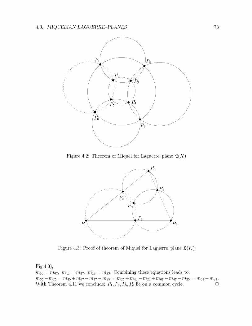
4.3. MIQUELIAN LAGUERRE–PLANES 73
P1
P2
P3
P4P5
P6
P7
P8
Figure 4.2: Theorem of Miquel for Laguerre–plane L(K)
P1
P2
P3
P4
P5
P6
P7
Figure 4.3: Proof of theorem of Miquel for Laguerre–plane L(K)
Fig.4.3),m16 = m67, m43 = m47, m12 = m23. Combining these equations leads to:m65−m25 = m45+m67−m47−m25 = m25+m43−m23+m67−m47−m25 = m61−m21.With Theorem 4.11 we conclude: P1, P2, P5, P6 lie on a common cycle. 2
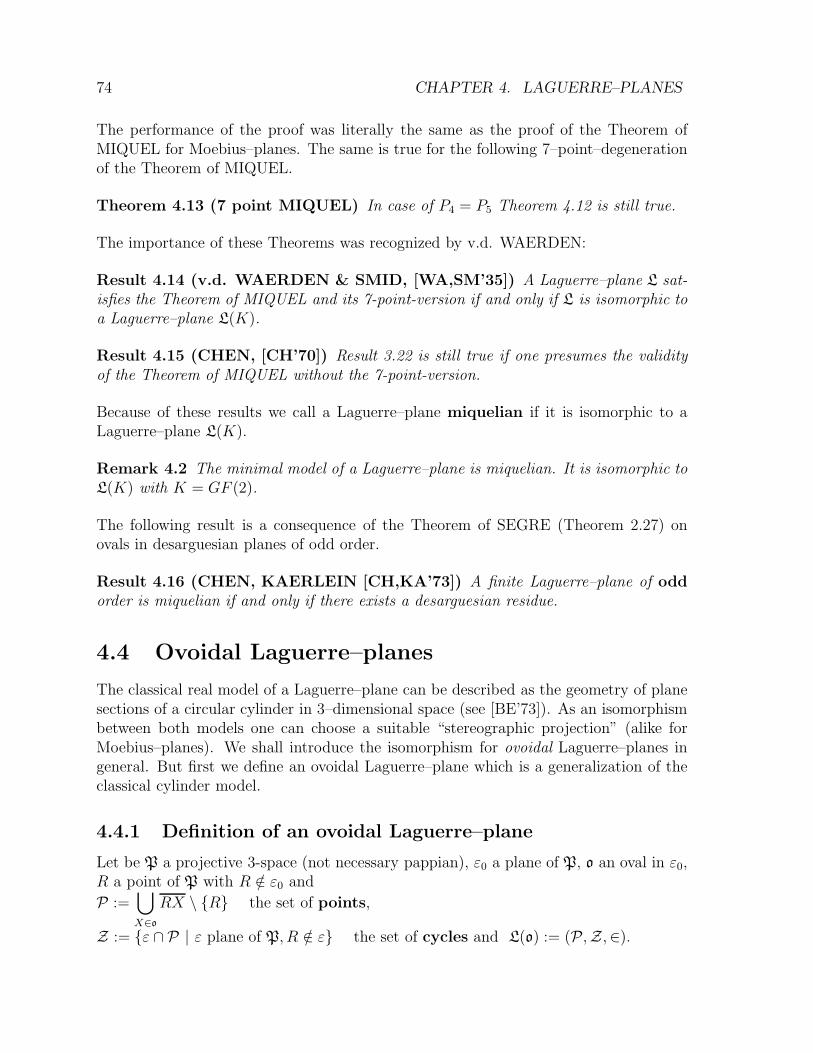
74 CHAPTER 4. LAGUERRE–PLANES
The performance of the proof was literally the same as the proof of the Theorem ofMIQUEL for Moebius–planes. The same is true for the following 7–point–degenerationof the Theorem of MIQUEL.
Theorem 4.13 (7 point MIQUEL) In case of P4 = P5 Theorem 4.12 is still true.
The importance of these Theorems was recognized by v.d. WAERDEN:
Result 4.14 (v.d. WAERDEN & SMID, [WA,SM’35]) A Laguerre–plane L sat-isfies the Theorem of MIQUEL and its 7-point-version if and only if L is isomorphic toa Laguerre–plane L(K).
Result 4.15 (CHEN, [CH’70]) Result 3.22 is still true if one presumes the validityof the Theorem of MIQUEL without the 7-point-version.
Because of these results we call a Laguerre–plane miquelian if it is isomorphic to aLaguerre–plane L(K).
Remark 4.2 The minimal model of a Laguerre–plane is miquelian. It is isomorphic toL(K) with K = GF (2).
The following result is a consequence of the Theorem of SEGRE (Theorem 2.27) onovals in desarguesian planes of odd order.
Result 4.16 (CHEN, KAERLEIN [CH,KA’73]) A finite Laguerre–plane of oddorder is miquelian if and only if there exists a desarguesian residue.
4.4 Ovoidal Laguerre–planes
The classical real model of a Laguerre–plane can be described as the geometry of planesections of a circular cylinder in 3–dimensional space (see [BE’73]). As an isomorphismbetween both models one can choose a suitable “stereographic projection” (alike forMoebius–planes). We shall introduce the isomorphism for ovoidal Laguerre–planes ingeneral. But first we define an ovoidal Laguerre–plane which is a generalization of theclassical cylinder model.
4.4.1 Definition of an ovoidal Laguerre–plane
Let be P a projective 3-space (not necessary pappian), ε0 a plane of P, o an oval in ε0,R a point of P with R /∈ ε0 and
P :=⋃
X∈o
RX \ {R} the set of points,
Z := {ε ∩ P | ε plane of P, R /∈ ε} the set of cycles and L(o) := (P,Z,∈).
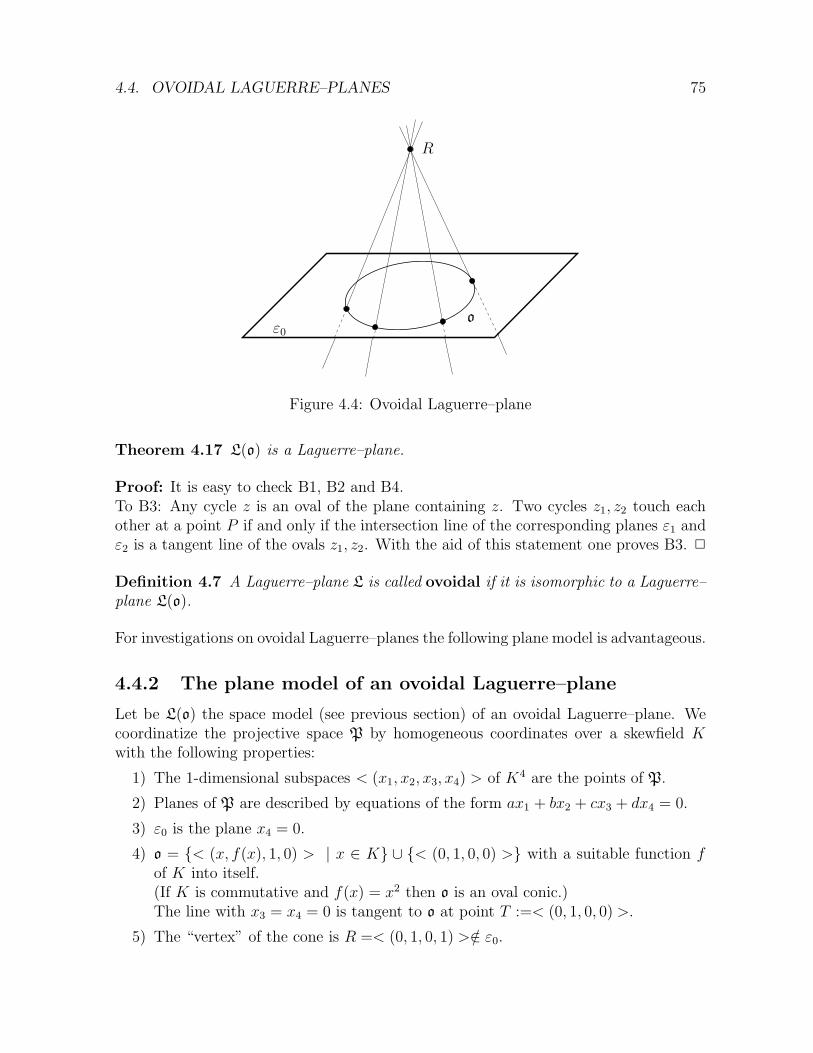
4.4. OVOIDAL LAGUERRE–PLANES 75
oε0
R
Figure 4.4: Ovoidal Laguerre–plane
Theorem 4.17 L(o) is a Laguerre–plane.
Proof: It is easy to check B1, B2 and B4.To B3: Any cycle z is an oval of the plane containing z. Two cycles z1, z2 touch eachother at a point P if and only if the intersection line of the corresponding planes ε1 andε2 is a tangent line of the ovals z1, z2. With the aid of this statement one proves B3. 2
Definition 4.7 A Laguerre–plane L is called ovoidal if it is isomorphic to a Laguerre–plane L(o).
For investigations on ovoidal Laguerre–planes the following plane model is advantageous.
4.4.2 The plane model of an ovoidal Laguerre–plane
Let be L(o) the space model (see previous section) of an ovoidal Laguerre–plane. Wecoordinatize the projective space P by homogeneous coordinates over a skewfield Kwith the following properties:
1) The 1-dimensional subspaces < (x1, x2, x3, x4) > of K4 are the points of P.
2) Planes of P are described by equations of the form ax1 + bx2 + cx3 + dx4 = 0.
3) ε0 is the plane x4 = 0.
4) o = {< (x, f(x), 1, 0) > | x ∈ K} ∪ {< (0, 1, 0, 0) >} with a suitable function fof K into itself.(If K is commutative and f(x) = x2 then o is an oval conic.)The line with x3 = x4 = 0 is tangent to o at point T :=< (0, 1, 0, 0) >.
5) The “vertex” of the cone is R =< (0, 1, 0, 1) >/∈ ε0.
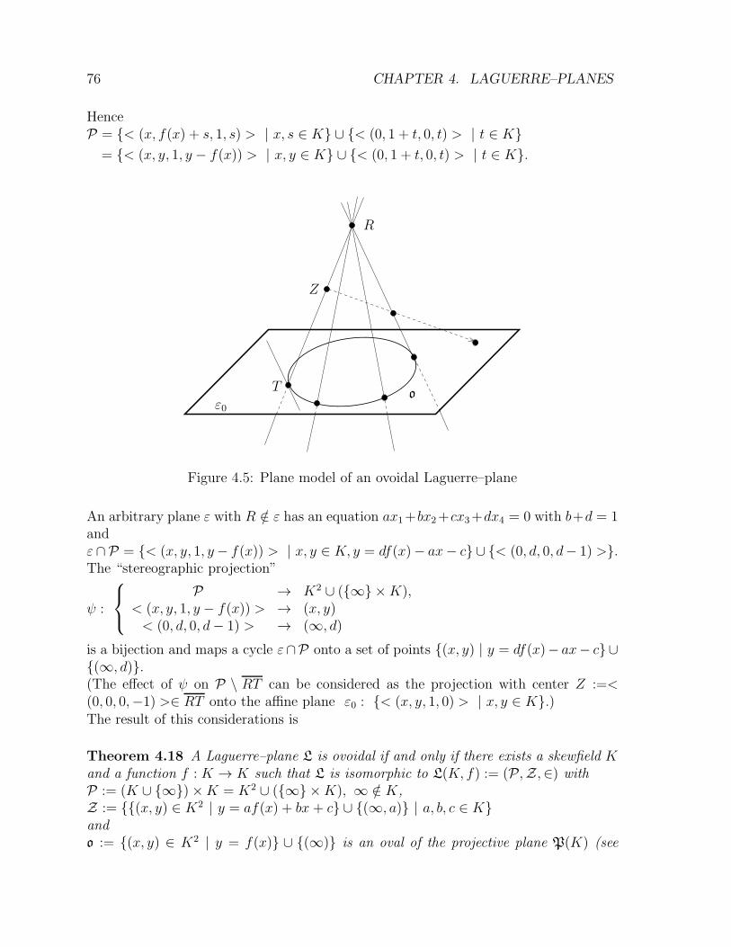
76 CHAPTER 4. LAGUERRE–PLANES
HenceP = {< (x, f(x) + s, 1, s) > | x, s ∈ K} ∪ {< (0, 1 + t, 0, t) > | t ∈ K}
= {< (x, y, 1, y − f(x)) > | x, y ∈ K} ∪ {< (0, 1 + t, 0, t) > | t ∈ K}.
oε0
R
T
Z
Figure 4.5: Plane model of an ovoidal Laguerre–plane
An arbitrary plane ε with R /∈ ε has an equation ax1+bx2+cx3+dx4 = 0 with b+d = 1andε∩P = {< (x, y, 1, y− f(x)) > | x, y ∈ K, y = df(x)− ax− c} ∪ {< (0, d, 0, d− 1) >}.The “stereographic projection”
ψ :
P → K2 ∪ ({∞} ×K),< (x, y, 1, y − f(x)) > → (x, y)< (0, d, 0, d− 1) > → (∞, d)
is a bijection and maps a cycle ε∩P onto a set of points {(x, y) | y = df(x)− ax− c}∪{(∞, d)}.(The effect of ψ on P \ RT can be considered as the projection with center Z :=<(0, 0, 0,−1) >∈ RT onto the affine plane ε0 : {< (x, y, 1, 0) > | x, y ∈ K}.)The result of this considerations is
Theorem 4.18 A Laguerre–plane L is ovoidal if and only if there exists a skewfield Kand a function f : K → K such that L is isomorphic to L(K, f) := (P,Z,∈) withP := (K ∪ {∞})×K = K2 ∪ ({∞} ×K), ∞ /∈ K,Z := {{(x, y) ∈ K2 | y = af(x) + bx + c} ∪ {(∞, a)} | a, b, c ∈ K}ando := {(x, y) ∈ K2 | y = f(x)} ∪ {(∞)} is an oval of the projective plane P(K) (see
4.4. OVOIDAL LAGUERRE–PLANES 77
Chapter 1).
Remark 4.3 a) Function f can be “normalized” such that f(0) = 0, f(1) = 1 andthe x-axis is a tangent line to o.
b) Any residue of an ovoidal Laguerre–plane is desarguesian.
4.4.3 Examples of ovoidal Laguerre–planes
For any oval o of a desarguesian projective plane we get a Laguerre–plane L(o). Manyovoidal Laguerre–planes have rather simple representations using the plane model:
1) An ovoidal Laguerre–plane L(K, f) with a normalized function f is miquelian ifand only if K is commutative and f(x) = x2. Hence an ovoidal Laguerre–planeL(o) is miquelian if and only if P is pappian and o is an oval conic.
2) a) For K = IR and f(x) = x4 the incidence structure L(K, f) is an ovoidalLaguerre–plane.b) For K = IR and f(x) = cosh x the incidence structure L(K, f) is an ovoidalLaguerre–plane.
3) For K = GF (2n), f(x) = x(2k) with k ∈ {1, 2, ..., n − 1} and k and n have no
common divisor the incidence structure L(K, f) is an ovoidal Laguerre–plane overa translation oval (see Section 2.7.1).
4) In case of “K skewfield, CharK = 2” and f is an injective function on K withf(0) = 0, f(1) = 1 which fulfills the functional equations
(i): f(x1 + x2) = f(x1) + f(x2), (ii): f(xf(x)−1) = f(x)−1, x 6= 0the incidence structure L(K, f) is an ovoidal Laguerre–plane over a Moufang oval(see Section 2.7.2).
Remark 4.4 In case of K = GF (2n), n ≥ 3, the system K := {{(x, y) ∈ K2 | y =ax2+bx+c} | a, b, c ∈ K} of curves can be embedded into two different (non isomorphic)Laguerre–planes:P := K2 ∪ ({∞} ×K), ∞ /∈ K,Z1 := {{(x, y) ∈ K2 | y = ax2 + bx+ c} ∪ {(∞, a)} | a, b, c ∈ K}Z2 := {{(x, y) ∈ K2 | y = ax2 + bx+ c} ∪ {(∞, b)} | a, b, c ∈ K}L1 := (P,Z1,∈) is the miquelian Laguerre–plane over K.L2 := (P,Z2,∈) is isomorphic to example 3) with k = n− 1. (The mapping (x, y) →(x(2
n−1), y) is the corresponding isomorphism.)
4.4.4 Automorphisms of an ovoidal Laguerre–plane L(K, f)
One easily checks the validity of
78 CHAPTER 4. LAGUERRE–PLANES
Lemma 4.19 Let be L(K, f) = (P,Z,∈) defined as in Theorem 4.18. The followingmappings are automorphisms of L(K, f):
(1) :
{
(x, y) → (x, y + s), x 6= ∞(∞, a) → (∞, a)
, s ∈ K (translation in A(∞,0))
(2) :
{
(x, y) → (x, y + sx), x 6= ∞(∞, a) → (∞, a)
, s ∈ K (shear in A(∞,0))
(3) :
{
(x, y) → (x, sy), x 6= ∞(∞, a) → (∞, sa)
, s ∈ K \ {0} (dilatation in A(∞,0))
(4) :
{
(x, y) → (x, y + sf(x)), x 6= ∞(∞, a) → (∞, a+ s)
, s ∈ K (translation in A(0,0))
Remark 4.5 a) (1) and (4) have exactly one generator as set of fixed points if s 6= 0.
b) (2) has exactly two generators as set of fixed points if s 6= 0.
c) (3) has exactly one cycle as set of fixed points if s 6= 1.
From Lemma 4.19 we get
Theorem 4.20 The automorphism group of an ovoidal Laguerre–plane operates tran-sitively on the set of cycles.
Further statements on the automorphisms of an ovoidal Laguerre–plane are containedin Section 4.6.
4.4.5 The bundle theorem for Laguerre–planes
Similar to ovoidal Moebius–planes the ovoidal Laguerre–planes can be characterized bythe Bundle Theorem:
Theorem 4.21 (Bundle Theorem) For an ovoidal Laguerre–plane L the followingstatement holds:Let be A1, A2, A3, A4, B1, B2, B3, B4 eight pairwise non parallel points. If 5 of the sixquadruples Qij := {Ai, Bi, Aj , Bj}, i < j, are concyclical on at least 4 cycles kij thenthis is true for the last quadruple, too (see Theorem 3.25).
Proof: Analogously to the Bundle Theorem for Moebius–planes (Theorem 3.25).
Result 4.22 (KAHN, [KH’80]) A Laguerre–plane is ovoidal if and only if the Bun-dle Theorem (Theorem 4.21) holds.
A further characterization will be given in Section 4.6.
Remark 4.6 Any Moebius–plane of even order is ovoidal and any Minkowski–planeof even order is miquelian. An analog statement for Laguerre–planes of even order isstill unknown.
4.5. NON OVOIDAL LAGUERRE–PLANES 79
4.5 Non ovoidal Laguerre–planes
The first non ovoidal Laguerre–planes were presented by MAURER in [MA’72]. Theyare isomorphic to Examples 1:
Example 4.1 (MAURER [MA’72], HARTMANN [HA’76])
Let be k ∈ IR with 0 < k 6= 1, a ◦ b :=
{
kab , if a, b < 0ab , other cases
.
and P := IR2 ∪ ({∞} × IR), ∞ /∈ IR,
Z1 := {{(x, y) ∈ IR2 | y = a ◦ x ◦ x+ b ◦ x+ c} ∪ {(∞, a)} | a, b, c ∈ IR}.
Then L1 := (P,Z1,∈) is a Laguerre–plane. The residue A(∞,0) is an affine MOULTONplane. Hence L1 is not ovoidal (see Remark b) to Theorem 4.18).
Example 4.2 (HARTMANN [HA’79a])
Let be r1, r2 ∈ IR with r1, r2 > 1, f the function on IR with f(x) :=
{
xr1 for x ≥ 0xr2 for x < 0
andP := IR
2 ∪ ({∞} × IR), ∞ /∈ IR,Z2 := {{(x, y) ∈ IR
2 | y = mx+ d} ∪ {(∞, 0)} | m, d ∈ IR}
∪ {{(x, y) ∈ IR2 | y = af(x− b) + c} ∪ {(∞, a)} | a, b, c ∈ IR, a 6= 0}.
Then L2 := (P,Z2,∈) is a Laguerre–plane.
For r1 = r2 = 2 L2 is the classical real Laguerre–plane.For any other case L2 is non ovoidal because there are desarguesian and non desargue-sian residues.
Example 4.3 (GROH [GR’74c])
Let be M = (PM ,ZM ,∈) a non ovoidal Moebius–plane as defined in Section 3.5 andP := set of oriented lines of affine plane A(IR),Z := IR
2 ∪ { oriented cycles ∈ ZM which not contain ∞}Incidence I is defined as follows:For any line g of A(IR) we have two oriented lines g1, g2 ∈ P. Analogously we get forany circle k ∈ ZM two oriented circles k1, k2 ∈ Z.gi ∈ P, (x, y) ∈ IR
2 : giI(x, y) ↔ (x, y) ∈ ggi ∈ P, kj ∈ Z \ IR2 : giIkj ↔ |g ∩ k| = 1 and orientations at touching point are thesameL := (P,Z, I) is a Laguerre–plane.If M is the classical real Moebius–plane then L is the original model of the classical realLaguerre–plane (see [BE’73]).For “most” cases L is non ovoidal (see [GR’74c]).
80 CHAPTER 4. LAGUERRE–PLANES
Example 4.4 (HARTMANN [HA’82b])
[HA’82b] contains non ovoidal examples over alternative division rings of characteristic2.
4.6 Automorphisms of Laguerre–planes
The close connection between a Laguerre–plane and affine planes (the residues are affineplanes !) motivates to look for automorphisms with at least one fixpoint. Such automor-phisms induce collineations of the residue at a fixpoint. In order to use results on thecoordinatization of affine planes we focus on automorphisms which induce translations,dilatations or shears in the residue of a fixpoint.
Definition 4.8 Let L = (P,Z,∈) be a Laguerre–plane.
a) An automorphism that fixes two non parallel points P,Q and any cycle containingP,Q is called dilatation at P,Q.Abbreviation for the group of dilatations: ∆(P,Q).
b) An automorphism that fixes a point P , any point of a generator e and a cycle zcontaining P is called dilatation at P, e with direction z.Group: ∆(P, e; z).
c) An automorphism that fixes the points of two generators e1, e2 and any generatoris called shear at e1, e2.Group: Σ(e1, e2).
d) An automorphism that fixes exactly the points of one generator e or P and anygenerator is called translation with axis e in direction E. (E is the set ofgenerators.)Group: T (e,E).
e) An automorphism that fixes exactly the points of a generator e or P and a cyclez is called translation with axis e in direction zGroup: T (e, z).
f) An automorphism that fixes any point of a cycle z is called dilatation at z.Group: ∆(z).
Obviously the following is true
Lemma 4.23 a) Any dilatation at P,Q induces a dilatation in AP at point Q.
b) Any dilatation at a point P , a generator e in direction z (containing P ) inducesa dilatation at line e in AP .
c) A shear at two generators e1, e2 induces a shear in any residue AP , P ∈ e1 ∪ e2.
d) Any translation with axis e and E–direction induces a translation in any residueAP , P ∈ e.
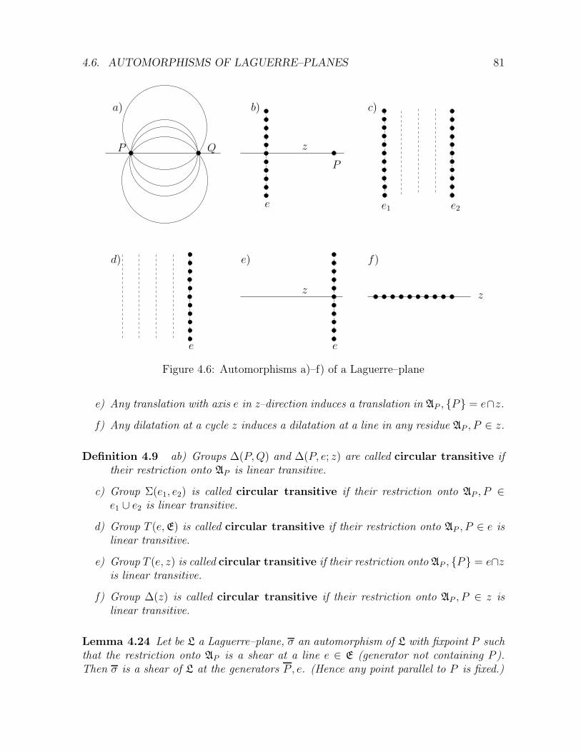
4.6. AUTOMORPHISMS OF LAGUERRE–PLANES 81
a) b) c)
d) e) f)
e
e e
e1 e2
z
z z
P
P
Q
Figure 4.6: Automorphisms a)–f) of a Laguerre–plane
e) Any translation with axis e in z–direction induces a translation in AP , {P} = e∩z.
f) Any dilatation at a cycle z induces a dilatation at a line in any residue AP , P ∈ z.
Definition 4.9 ab) Groups ∆(P,Q) and ∆(P, e; z) are called circular transitive iftheir restriction onto AP is linear transitive.
c) Group Σ(e1, e2) is called circular transitive if their restriction onto AP , P ∈e1 ∪ e2 is linear transitive.
d) Group T (e,E) is called circular transitive if their restriction onto AP , P ∈ e islinear transitive.
e) Group T (e, z) is called circular transitive if their restriction onto AP , {P} = e∩zis linear transitive.
f) Group ∆(z) is called circular transitive if their restriction onto AP , P ∈ z islinear transitive.
Lemma 4.24 Let be L a Laguerre–plane, σ an automorphism of L with fixpoint P suchthat the restriction onto AP is a shear at a line e ∈ E (generator not containing P ).Then σ is a shear of L at the generators P, e. (Hence any point parallel to P is fixed.)
82 CHAPTER 4. LAGUERRE–PLANES
Proof: If σ fixes any point of the generator e 6= P and if Q ∈ e then σ induces in AQ acollineation σQ which fixes any generator. If σQ is not the identity the set of fixpointsis at least P and at most P . Hence σQ is a shear in AQ and σ a shear at e, P in L. 2
It is unknown if Lemma 4.24 is true for translations, too.Using additional assumptions a similar result can be achieved:
Lemma 4.25 Let be L a Laguerre–plane, τ an automorphism of L with fixpoint P suchthat the restriction onto AP is a translation. Then τ is a translation of L. (Hence anypoint parallel to P is fixed.) if one of the following conditions is fulfilled:
a) There is a point Q /∈ P such that ∆(P,Q) is circular transitive.
b) AP is a translation plane of characteristic 6= 2 and any reflection at a point (inAP ) is induced by a dilatation (of L) at a pair of points.
c) L is finite and τ involutorial.
d) L is ovoidal of characteristic 2.
Proof: see [HA’82b], Lemma 2.2.
Definition 4.10 Let be L a Laguerre–plane, σ an involutorial automorphism
a) with two fixpoints P,Q. Then σ is called reflection at P,Q.
b) whose set of fixpoints consists of two generators e1 6= e2 and which leaves one cycleinvariant is called reflection at e1, e2.
c) whose fixpoints are the points of a cycle z is called reflection at z.
For involutorial automorphisms the following statements hold:
Lemma 4.26 a) A reflection σPQ at two non parallel points P,Q is a dilatation atP,Q.
b) An involutorial dilatation σ ∈ ∆(P, e; z) is a reflection at the generators e, P .
c) An involutorial dilatation τ whose set of fixpoints are the points of a generator eis a translation (of L) with axis e.
d) An involutorial automorphism σ whose set of fixpoints are the points of two gen-erators e1 6= e2 is a reflection at e1, e2 or a shear at e1, e2.
Proof: see [HA’82b], Lemma 2.3.
4.6. AUTOMORPHISMS OF LAGUERRE–PLANES 83
4.6.1 Transitivity properties of ovoidal Laguerre–planes
Theorem 4.27 For an ovoidal Laguerre–plane the following statements are true:
a) Any group T (e;E) of translations in E–direction is circular transitive.
b) Any group Σ(e1, e2) of shears is circular transitive.
b) Any group ∆(z) of dilatations is circular transitive.
d) In case of characteristic 6= 2 for any cycle there is a reflection.
Proof: The statements can be checked easily using the plane model of an ovoidalLaguerre–plane and Lemma 4.19. 2
For a miquelian Laguerre–plane we get additionally
Theorem 4.28 For a miquelian Laguerre–plane the following statements are true:
a) Any group ∆(P,Q) of dilatations at pairs of points is circular transitive.
b) Any group ∆(P, e; z) of dilatations at generators is circular transitive.
c) Any group T (e; z) of translations is circular transitive.
d) In case of characteristic 6= 2 for any pair of non parallel points there is a reflection.
e) In case of characteristic 6= 2 for any pair of generators e1 6= e2 and cycle z thereis exactly one reflection at e1, e2 which leaves z invariant.
Proof: Use Lemma 4.7 and Lemma 4.8. 2
Theorem 4.29 For an ovoidal Laguerre–plane over a Moufang oval any group T (e; z)of translations in the direction of a cycle is circular transitive.
Proof: Let be L(K, f) an ovoidal Laguerre–plane as defined in Theorem 4.18 overa Moufang oval (see Section 4.4.3). From the property f(x1 + x2) = f(x1) + f(x2)we get the circular transitivity of T (e; z) for (∞, 0). The statement for other groupsT (e; z) yields can be achieved using the following mapping which is an automorphismof L(K, f):
(x, y) → (xf(x)−1, yf(x)−1), x 6= 0(0, y) → (∞, y)(∞, a) → (0, a)
(Take notice of the functional equation f(xf(x)−1) = f(x)−1 for x 6= 0.) 2
Theorem 4.30 For a finite and ovoidal Laguerre–plane over a translation oval thereexists a generator e0 such that
a) any translation group T (e0; z) is circular transitive,
b) any dilatation group ∆(P,Q) with P ∈ e0 is circular transitive,
84 CHAPTER 4. LAGUERRE–PLANES
c) any dilatation group ∆(P, e; z) with P ∈ e0 is circular transitive.
Proof: An ovoidal Laguerre–plane over a finite translation oval can be represented asL(K, f) with K = GF (2n) and function f(x) = x(2
k) (see Section 4.4.3). We choosee0 = (∞, 0).To a): From the property f(x1 + x2) = f(x1) + f(x2) we get the circular transitivity ofany group T (e0; z).To b): Because of a) and Theorem 4.27 it suffice to discuss the case with P = (∞, 0)and Q = (0, 0). Obviously any mapping
{
(x, y) → (sx, sy), s 6= 0(∞, a) → (∞, asf(s)−1)
is an automorphism of L(K, f) and ∆(P,Q) is circular transitive.To c): Because of theorem 4.20 and statement a) we confine to the case with P = (∞, 0),e is generator x = 0 and z cycle y = 0. For this case it is simple to check the circulartransitivity of ∆(P, e; z). 2
The following results use the properties above to characterize certain classes of ovoidalLaguerre–planes.
Result 4.31 (KREBS, MAURER [MA’77], Satz 6) A Laguerre–plane L = (P,Z,∈) is miquelian if and only if any dilatation group ∆(z), z ∈ Z is circular transitive.
Result 4.32 (HARTMANN [HA’82b], Satz 7) A Laguerre–plane L = (P,Z,∈)is miquelian if and only if any dilatation group ∆(P,Q), P, Q ∈ P is circular transitive.
In case of characteristic 6= 2 we have stronger results:
Result 4.33 A Laguerre–plane L = (P,Z,∈) of characteristic 6= 2 is miquelian if andonly if
a) for any pair of non parallel points P,Q there is exactly one reflection at P,Q. (seeMAURER [MA’78])
b) There is a generator e0 such that any dilatation group ∆(P,Q), P ∈ e0 is circulartransitive and contains an involution. (see HARTMANN [HA’82b], Satz 8)
c) There is a generator e0 such that any dilatation group ∆(P, e; z), P ∈ e0 is circulartransitive and contains an involution. (see HARTMANN [HA’82b], Satz 10)
Results 4.33 can not be extended to characteristic 6= 2:
Result 4.34 (HARTMANN [HA’82b], Satz 9, Satz 11) A finite Laguerre–planeL = (P,Z,∈) of even order is ovoidal over a translation oval if there is a generatore0 such that one of the following statements hold:
a) Any dilatation group ∆(P,Q), P ∈ e0 is circular transitive.
4.6. AUTOMORPHISMS OF LAGUERRE–PLANES 85
b) Any dilatation group ∆(P, e; z), P ∈ e0 is circular transitive.
Ovoidal Laguerre–planes over Moufang ovals can be characterized by translations:
Result 4.35 (HARTMANN [HA’82b], Satz 4) A Laguerre–plane L = (P,Z,∈)is ovoidal over a Moufang oval if
i) at least one residue is desarguesian of characteristic 2,
ii) any translation group T (e; z) is circular transitive.
Property i) of the last result is essential and can not be omitted. There are non ovoidalLaguerre–planes which fulfill property ii) (see [HA’82b], Remark to Satz 14).But for finite Laguerre–planes we have
Result 4.36 (HARTMANN [HA’82b], Satz 1) A finite Laguerre–plane L = (P,Z,∈) is miquelian if and only if any translation group T (e; z) is circular transitive.
86 CHAPTER 4. LAGUERRE–PLANES
Chapter 5
MINKOWSKI–PLANES
Literature: [BE’73]
5.1 The classical real Minkowski–plane
Applying the pseudo-euclidean distance dP (P1, P2) = (x1−x2)2−(y1−y2)
2 on two pointsPi = (xi.yi) (instead of the euclidean one) we get the geometry of hyperbolas, becausea pseudoeuclidean circle {P ∈ IR
2 | dP (P,M) = r} is a hyperbola with midpoint M .By a suitable coordinate transformation we can rewrite the pseudo-euclidean distanceas d′P (P1, P2) = (x1 − x2)(y1 − y2). Now the hyperbolas have asymptotes parallel tothe coordinate axes. The following completion (see Moebius– and Laguerre–planes)“homogenizes” the geometry of hyperbolas:P := (IR ∪ {∞})2 = IR
2 ∪ ({∞} × IR) ∪ (IR× {∞}) ∪ {(∞,∞)} , ∞ /∈ IR, the set ofpoints,Z := {{(x, y) ∈ IR
2 | y = ax+ b} ∪ {(∞,∞)} | a, b ∈ IR, a 6= 0}∪ {{(x, y) ∈ IR
2 |y = ax−b
+ c, x 6= b} ∪ {(b,∞), (∞, c)} | a, b, c ∈ IR, a 6= 0}, the setof cycles.The incidence structure (P,Z,∈) is called classical real Minkowski–plane.
Remark 5.1 One should not confuse the Minkowski–plane defined above with the Minkowski–plane founded on reflections (see [LI’78]).
Obviously the set of cycles can be described by the group PGL(2, IR) operating onIR ∪ {∞}:Z = {{(x, y) ∈ P | y = π(x)} | π ∈ PGL(2, IR)}.A cycle defined by equation y = ax+ b is represented by a permutation π ∈ PGL(2, IR)with π(∞) = ∞ and a cycle defined by equation y = a
x−b+ c is represented by
π ∈ PGL(2, IR) with π(∞) = c and π(b) = ∞.
Two points (x1, y1) 6= (x2, y2) can not be connected by a cycle if and only if x1 = x2 ory1 = y2. Similar to the parallel relation for Laguerre–planes we define:
87
88 CHAPTER 5. MINKOWSKI–PLANES
Two points P1, P2 are (+)-parallel (P1 ‖+ P2) if x1 = x2 and (-)-parallel (P1 ‖− P2)if y1 = y2. Both these relations are equivalence relations on the set of points.Two points P1, P2 are called parallel (P1 ‖ P2) if P1 ‖+ P2 or P1 ‖− P2.
Lemma 5.1 The mappings (x, y) → (y, x) and (x, y) → (α(x), β(y), α, β ∈ PGL(2, IR)are automorphisms of (P,Z,∈) (see Section 5.3).
With help of the last lemma we find:
Lemma 5.2 1. For any pair of non parallel points A,B there is exactly one point Cwith A ‖+ C ‖− B.
2. For any point P and any cycle z there are exactly two points A,B ∈ z withA ‖+ P ‖− B.
3. For any three points A,B,C, pairwise non parallel, there is exactly one cycle zwhich contains A,B,C.
4. For any cycle z, any point P ∈ z and any point Q,P 6‖ Q and Q /∈ z there existsexactly one cycle z′ such that z ∩ z′ = {P}, i.e. z touches z′ at point P.
Like the classical Moebius– and Laguerre–planes Minkowski–planes can be described asthe geometry of plane sections of a suitable quadric. But in this case the quadric livesin projective 3-space: The classical real Minkowski–plane is isomorphic to the geometryof plane sections of a hyperboloid of one sheet (not degenerated quadric of index 2). Theisomorphism will be introduced in Section 5.3.
5.2 The axioms of a Minkowski–plane
Definition 5.1 Let be (P,Z; ‖+, ‖−,∈) an incidence structure with the set P of points,the set Z of cycles and two equivalence relations ‖+ ((+)-parallel) and ‖− ((-)-parallel)on set P.For P ∈ P we define: P+ := {Q ∈ P | Q ‖+ P} and P− := {Q ∈ P | Q ‖− P}.An equivalence class P+ or P− is called (+)-generator and (-)-generator, respec-tively. Furthermore we define: E+ := {P+ | P ∈ P}, E− := {P− | P ∈ P} andE := E+ ∪ E−.Two points A,B are called parallel (A ‖ B) if A ‖+ B or A ‖− B.
Definition 5.2 An incidence structure M := (P,Z; ‖+, ‖−,∈) is called Minkowski–plane if the following axioms hold:
C1: For any pair of non parallel points A,B there is exactly one point C with A ‖+C ‖− B.
C2: For any point P and any cycle z there are exactly two points A,B ∈ z withA ‖+ P ‖− B.
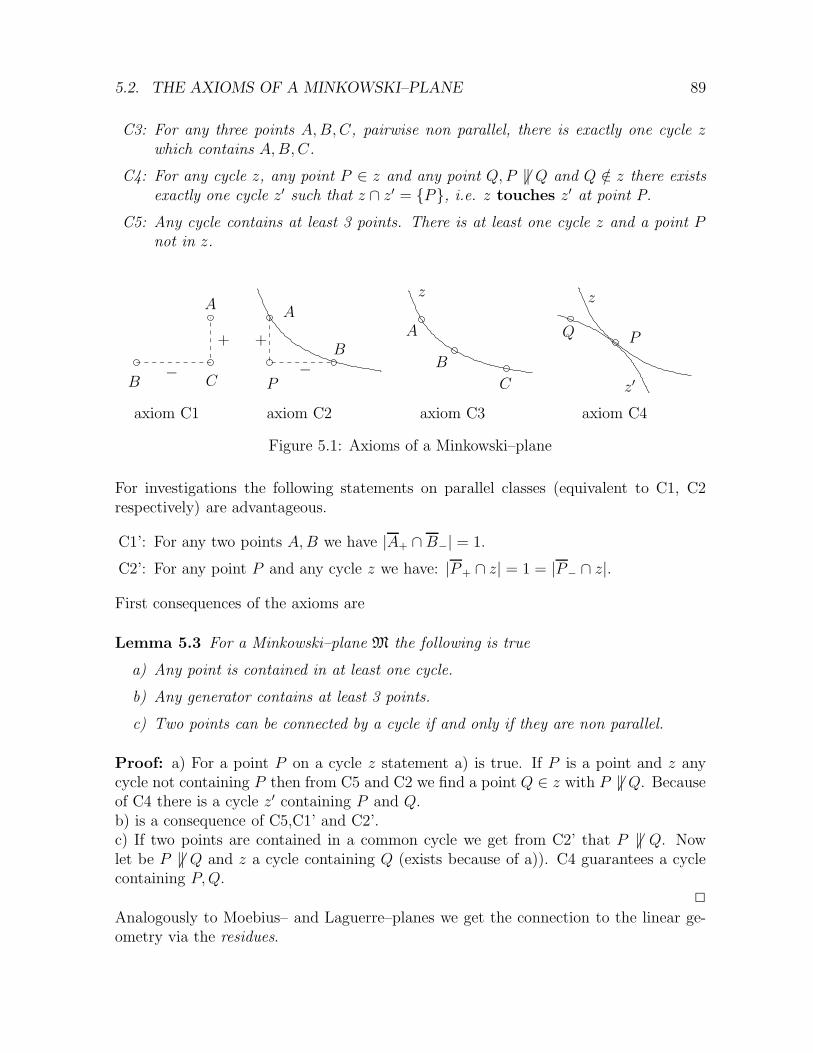
5.2. THE AXIOMS OF A MINKOWSKI–PLANE 89
C3: For any three points A,B,C, pairwise non parallel, there is exactly one cycle zwhich contains A,B,C.
C4: For any cycle z, any point P ∈ z and any point Q,P 6‖ Q and Q /∈ z there existsexactly one cycle z′ such that z ∩ z′ = {P}, i.e. z touches z′ at point P.
C5: Any cycle contains at least 3 points. There is at least one cycle z and a point Pnot in z.
AA
A
BB
B CC
zz
z′
P
P
Q++
−−
axiom C1 axiom C2 axiom C3 axiom C4
Figure 5.1: Axioms of a Minkowski–plane
For investigations the following statements on parallel classes (equivalent to C1, C2respectively) are advantageous.
C1’: For any two points A,B we have |A+ ∩ B−| = 1.
C2’: For any point P and any cycle z we have: |P+ ∩ z| = 1 = |P− ∩ z|.
First consequences of the axioms are
Lemma 5.3 For a Minkowski–plane M the following is true
a) Any point is contained in at least one cycle.
b) Any generator contains at least 3 points.
c) Two points can be connected by a cycle if and only if they are non parallel.
Proof: a) For a point P on a cycle z statement a) is true. If P is a point and z anycycle not containing P then from C5 and C2 we find a point Q ∈ z with P 6‖ Q. Becauseof C4 there is a cycle z′ containing P and Q.b) is a consequence of C5,C1’ and C2’.c) If two points are contained in a common cycle we get from C2’ that P 6‖ Q. Nowlet be P 6‖ Q and z a cycle containing Q (exists because of a)). C4 guarantees a cyclecontaining P,Q.
2
Analogously to Moebius– and Laguerre–planes we get the connection to the linear ge-ometry via the residues.
90 CHAPTER 5. MINKOWSKI–PLANES
Definition 5.3 For a Minkowski–plane M = (P,Z; ‖+, ‖−,∈) and P ∈ P we define
AP := (P \ P, {z \ {P} | P ∈ z ∈ Z} ∪ {E \ P | E ∈ E \ {P+, P−}},∈)
and call it the residue at point P.
An immediate consequence of axioms C1 - C4 and C1’, C2’ are the following two theo-rems.
Theorem 5.4 For a Minkowski–plane M = (P,Z; ‖+, ‖−,∈) we have:a) Any residue is an affine plane.b) For any cycle z and any point P ∈ P \ z the set z \ P is a hyperbolic curve of AP
(see Section 2.1)
Theorem 5.5 Let be M = (P,Z; ‖+, ‖−,∈) an incidence structure with two equivalencerelations ‖+ and ‖− on the set P of points (see above). Then:M is a Minkowski–plane if and only if for any point P the incidence structure (residue)
AP := (P \ P, {z \ {P} | P ∈ z ∈ Z} ∪ {E \ P | E ∈ E \ {P+, P−}},∈)
is an affine plane.
The minimal model of a Minkowski–plane can be established over the set K :={0, 1,∞} of three elements:
P := K2, Z := {{(a1, b1), (a2, b2), (a3, b3)} | {a1, a2, a3} = {b1, b2, b3} = K},
(x1, y1) ‖+ (x2, y2) if and only if x1 = x2 and (x1, y1) ‖− (x2, y2) if and only ify1 = y2.Hence: |P| = 9 and |Z| = 6.
For finite Minkowski-planes we get from C1’, C2’:
Lemma 5.6 Let be M = (P,Z; ‖+, ‖−,∈) a finite Minkowski–plane, i.e. |P| <∞. Forany pair of cycles z1, z2 and any pair of generators e1, e2 we have: |z1| = |z2| = |e1| =|e2|.
This gives rise of
Definition 5.4 For a finite Minkowski–plane M and a cycle z of M we call the integern = |z| − 1 the order of M.
Simple combinatorial considerations yield (see [BP’83])
Lemma 5.7 For a finite Minkowski–plane M = (P,Z; ‖+, ‖−,∈) the following is true:a) Any residue (affine plane) has order n.b) |P| = (n + 1)2, c) |Z| = (n+ 1)n(n− 1).
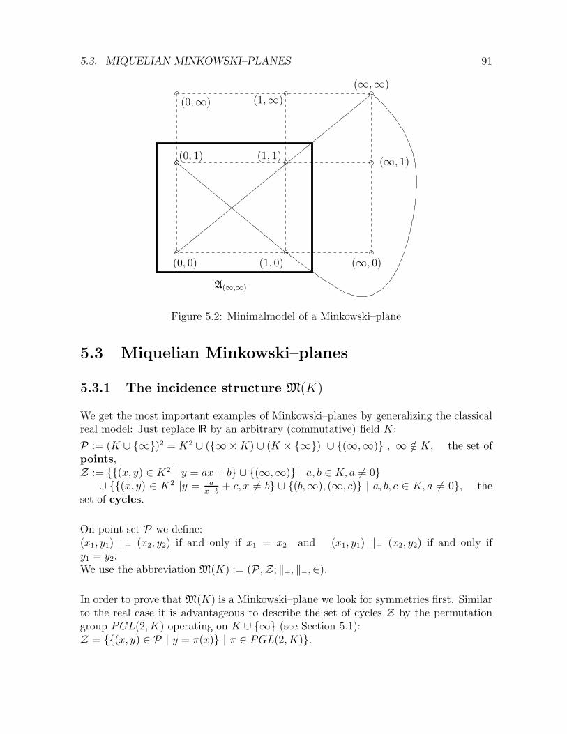
5.3. MIQUELIAN MINKOWSKI–PLANES 91
(0, 0)
(0, 1) (1, 1)
(1, 0)
(0,∞) (1,∞)
(∞,∞)
(∞, 0)
(∞, 1)
A(∞,∞)
Figure 5.2: Minimalmodel of a Minkowski–plane
5.3 Miquelian Minkowski–planes
5.3.1 The incidence structure M(K)
We get the most important examples of Minkowski–planes by generalizing the classicalreal model: Just replace IR by an arbitrary (commutative) field K:
P := (K ∪ {∞})2 = K2 ∪ ({∞×K) ∪ (K × {∞}) ∪ {(∞,∞)} , ∞ /∈ K, the set ofpoints,Z := {{(x, y) ∈ K2 | y = ax+ b} ∪ {(∞,∞)} | a, b ∈ K, a 6= 0}
∪ {{(x, y) ∈ K2 |y = ax−b
+ c, x 6= b} ∪ {(b,∞), (∞, c)} | a, b, c ∈ K, a 6= 0}, theset of cycles.
On point set P we define:(x1, y1) ‖+ (x2, y2) if and only if x1 = x2 and (x1, y1) ‖− (x2, y2) if and only ify1 = y2.We use the abbreviation M(K) := (P,Z; ‖+, ‖−,∈).
In order to prove that M(K) is a Minkowski–plane we look for symmetries first. Similarto the real case it is advantageous to describe the set of cycles Z by the permutationgroup PGL(2, K) operating on K ∪ {∞} (see Section 5.1):Z = {{(x, y) ∈ P | y = π(x)} | π ∈ PGL(2, K)}.
92 CHAPTER 5. MINKOWSKI–PLANES
5.3.2 Automorphisms of M(K). M(K) is a Minkowski–plane
Definition 5.5 Any automorphism of the incidence structure (P,Z,∈) is called auto-morphism of M(K).
Analogously to the real case we get
Lemma 5.8 The following permutations of point set P are automorphisms of M(K):
a) (x, y) → (y, x),
b) (x, y) → (α(x), β(y)), with α, β ∈ PGL(2, K),
c) (x, y) → (κ(x), κ(y)), with κ(∞) = ∞ and the restriction of κ onto K is anautomorphism of the field (K,+, ·).
The proof is a consequence of the fact “PGL(2, K) is a group” and κπκ−1 ∈ PGL(2, K)for any κ, π ∈ PGL(2, K).From the 3–transitivity of group PGL(2, K) we get
Lemma 5.9 The automorphism group of M(K) operates transitively ona) the set of triples of pairwise non parallel points andb) the set of cycles,either.
The following list contains some typical automorphisms of structure M(K). We defineany automorphism by its action on K2 and extend it using the conventions:k · ∞ = ∞, k +∞ = ∞, 1/∞ = 0, 1/0 = ∞.
(1) (x, y) → (x+ s, y + t), s, t ∈ K,
(2) (x, y) → (sx, y), s ∈ K \ {0},
(3) (x, y) → (x, ty), t ∈ K \ {0},
(4) (x, y) → ( 1x, y), (CharK 6= 2: reflection in A(1,0) at line x = −1,
CharK = 2: translation in A(1,0)),
(5) (x, y) → (x, 1y), (analogously to (4))
(6) (x, y) → ( 1x, 1y), (CharK 6= 2: reflection in A(1,1) at point (−1,−1),
CharK = 2: translation in A(1,1)),
(7) (x, y) → (y, x), (CharK 6= 2: reflection in A(∞,∞) at line y = x,CharK = 2: shear in A(∞,∞) at line y = x).
Analogously to the Laguerre case one proves
Theorem 5.10 a) M(K) is a Minkowski–plane.b) The automorphisms of Lemma 5.8 generate the full group of automorphisms of M(K).
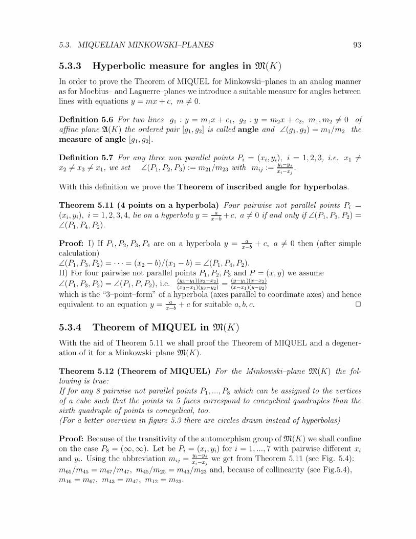
5.3. MIQUELIAN MINKOWSKI–PLANES 93
5.3.3 Hyperbolic measure for angles in M(K)
In order to prove the Theorem of MIQUEL for Minkowski–planes in an analog manneras for Moebius– and Laguerre–planes we introduce a suitable measure for angles betweenlines with equations y = mx+ c, m 6= 0.
Definition 5.6 For two lines g1 : y = m1x + c1, g2 : y = m2x + c2, m1, m2 6= 0 ofaffine plane A(K) the ordered pair [g1, g2] is called angle and ∠(g1, g2) = m1/m2 themeasure of angle [g1, g2].
Definition 5.7 For any three non parallel points Pi = (xi, yi), i = 1, 2, 3, i.e. x1 6=x2 6= x3 6= x1, we set ∠(P1, P2, P3) := m21/m23 with mij :=
yi−yjxi−xj
.
With this definition we prove the Theorem of inscribed angle for hyperbolas.
Theorem 5.11 (4 points on a hyperbola) Four pairwise not parallel points Pi =(xi, yi), i = 1, 2, 3, 4, lie on a hyperbola y = a
x−b+ c, a 6= 0 if and only if ∠(P1, P3, P2) =
∠(P1, P4, P2).
Proof: I) If P1, P2, P3, P4 are on a hyperbola y = ax−b
+ c, a 6= 0 then (after simplecalculation)∠(P1, P3, P2) = · · · = (x2 − b)/(x1 − b) = ∠(P1, P4, P2).II) For four pairwise not parallel points P1, P2, P3 and P = (x, y) we assume
∠(P1, P3, P2) = ∠(P1, P, P2), i.e.(y3−y1)(x3−x2)(x3−x1)(y3−y2)
= (y−y1)(x−x2)(x−x1)(y−y2)
which is the “3–point–form” of a hyperbola (axes parallel to coordinate axes) and henceequivalent to an equation y = a
x−b+ c for suitable a, b, c. 2
5.3.4 Theorem of MIQUEL in M(K)
With the aid of Theorem 5.11 we shall proof the Theorem of MIQUEL and a degener-ation of it for a Minkowski–plane M(K).
Theorem 5.12 (Theorem of MIQUEL) For the Minkowski–plane M(K) the fol-lowing is true:If for any 8 pairwise not parallel points P1, ..., P8 which can be assigned to the verticesof a cube such that the points in 5 faces correspond to concyclical quadruples than thesixth quadruple of points is concyclical, too.(For a better overview in figure 5.3 there are circles drawn instead of hyperbolas)
Proof: Because of the transitivity of the automorphism group of M(K) we shall confineon the case P8 = (∞,∞). Let be Pi = (xi, yi) for i = 1, ..., 7 with pairwise different xiand yi. Using the abbreviation mij =
yi−yjxi−xj
we get from Theorem 5.11 (see Fig. 5.4):
m65/m45 = m67/m47, m45/m25 = m43/m23 and, because of collinearity (see Fig.5.4),m16 = m67, m43 = m47, m12 = m23.
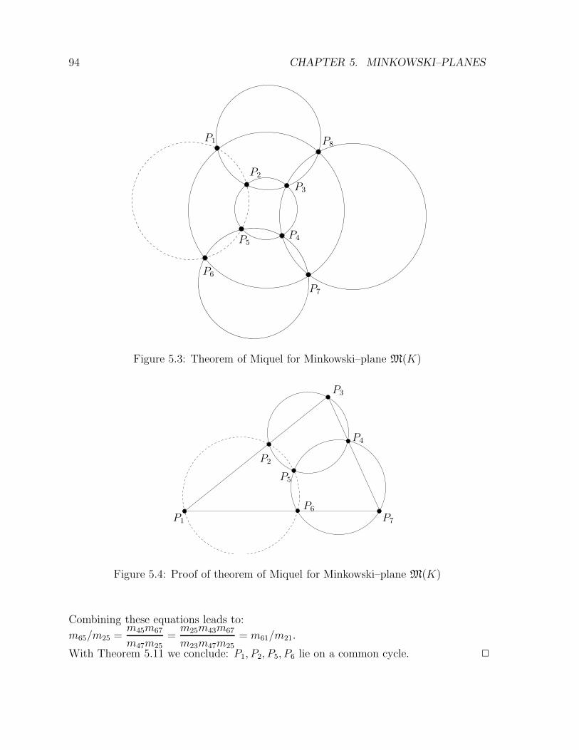
94 CHAPTER 5. MINKOWSKI–PLANES
P1
P2
P3
P4P5
P6
P7
P8
Figure 5.3: Theorem of Miquel for Minkowski–plane M(K)
P1
P2
P3
P4
P5
P6
P7
Figure 5.4: Proof of theorem of Miquel for Minkowski–plane M(K)
Combining these equations leads to:
m65/m25 =m45m67
m47m25=m25m43m67
m23m47m25= m61/m21.
With Theorem 5.11 we conclude: P1, P2, P5, P6 lie on a common cycle. 2
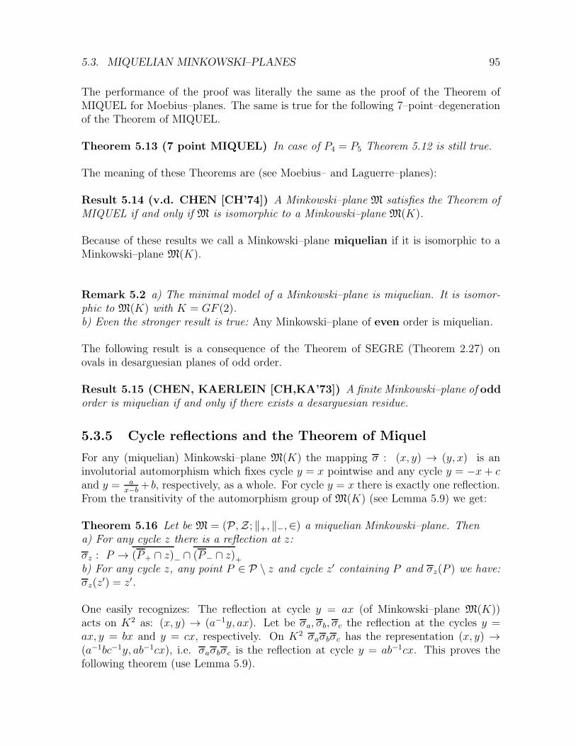
5.3. MIQUELIAN MINKOWSKI–PLANES 95
The performance of the proof was literally the same as the proof of the Theorem ofMIQUEL for Moebius–planes. The same is true for the following 7–point–degenerationof the Theorem of MIQUEL.
Theorem 5.13 (7 point MIQUEL) In case of P4 = P5 Theorem 5.12 is still true.
The meaning of these Theorems are (see Moebius– and Laguerre–planes):
Result 5.14 (v.d. CHEN [CH’74]) A Minkowski–plane M satisfies the Theorem ofMIQUEL if and only if M is isomorphic to a Minkowski–plane M(K).
Because of these results we call a Minkowski–plane miquelian if it is isomorphic to aMinkowski–plane M(K).
Remark 5.2 a) The minimal model of a Minkowski–plane is miquelian. It is isomor-phic to M(K) with K = GF (2).b) Even the stronger result is true: Any Minkowski–plane of even order is miquelian.
The following result is a consequence of the Theorem of SEGRE (Theorem 2.27) onovals in desarguesian planes of odd order.
Result 5.15 (CHEN, KAERLEIN [CH,KA’73]) A finite Minkowski–plane of oddorder is miquelian if and only if there exists a desarguesian residue.
5.3.5 Cycle reflections and the Theorem of Miquel
For any (miquelian) Minkowski–plane M(K) the mapping σ : (x, y) → (y, x) is aninvolutorial automorphism which fixes cycle y = x pointwise and any cycle y = −x+ cand y = a
x−b+ b, respectively, as a whole. For cycle y = x there is exactly one reflection.
From the transitivity of the automorphism group of M(K) (see Lemma 5.9) we get:
Theorem 5.16 Let be M = (P,Z; ‖+, ‖−,∈) a miquelian Minkowski–plane. Thena) For any cycle z there is a reflection at z:
σz : P → (P+ ∩ z)− ∩ (P− ∩ z)+b) For any cycle z, any point P ∈ P \ z and cycle z′ containing P and σz(P ) we have:σz(z
′) = z′.
One easily recognizes: The reflection at cycle y = ax (of Minkowski–plane M(K))acts on K2 as: (x, y) → (a−1y, ax). Let be σa, σb, σc the reflection at the cycles y =ax, y = bx and y = cx, respectively. On K2 σaσbσc has the representation (x, y) →(a−1bc−1y, ab−1cx), i.e. σaσbσc is the reflection at cycle y = ab−1cx. This proves thefollowing theorem (use Lemma 5.9).

96 CHAPTER 5. MINKOWSKI–PLANES
Theorem 5.17 (Theorem on 3 reflections) LetM be a miquelian Minkowski–plane,P,Q a pair of non parallel points and σ1, σ2, σ3 the reflections at three cycles z1, z2, z3containing P,Q. Then σ1σ2σ3 is the reflection at a cycle z4 containing P,Q.
For Minkowski–planes M(K) the reflections at cycles passing (∞,∞) induce reflectionsat lines (involutorial collineations) at lines y = ax+ b, a 6= 0 of affine plane A(K)(∞,∞).Let be Σ∞ the set of such line reflections. For any two non parallel points P,Q ∈ K2
there is exactly one σ ∈ Σ∞ with σ(P ) = Q. The corresponding line is called bisectorof P,Q. In case of CharK 6= 2 the bisector of P,Q intersects the line through P,Q. Incase of CharK = 2 the bisector is parallel to the line through P,Q. For two reflectionsσ1, σ2 ∈ Σ∞ corresponding to two parallel lines σ1σ2 is a translation. If σ1, σ2 arereflections of non parallel lines containing point A = (x0, y0), then σ1σ2 is a Minkowskirotation at point A, i.e. σ1σ2 fixes the hyperbola y = a
x−x0+ y0 (because of Theorem
5.16 b)) and A is the unique fixpoint in case of σ1 6= σ2. Especially we get
Lemma 5.18 Let be P1, P2, P3, P4 four non parallel points of residue A(∞,∞) of Minkowski–plane M(K), which are not collinear, and σik ∈ Σ∞ the reflection which exchanges Pi
and Pk. Then: P1, P2, P3, P4 lie on a hyperbola y = ax−b
+c if and only if σ12σ23σ34 = σ14.
Proof: I) If P1, P2, P3, P4 are on a hyperbola y = ax−x0
+y0 one proves by an easy calcu-lation, that all bisector lines (of the points) contain point P = (x0, y0). With Theorem5.17 we get the statement.II) In case of σ12σ23σ34 = σ14 the Minkowski– rotation ψ : σ12σ23 = σ14σ43 leaves thehyperbola h determined by P1, P2, P3 and h′ determined by P1, P3, P4, respectively, in-variant. Because for any Minkowski–rotation and any point P , different from the centerof rotation, there is exactly one fix–hyperbola containing P . Hence we have h = h′ andthe existence of a common hyperbola. 2
Remark 5.3 With help Lemma of 5.18 one gets a further proof of the Theorem ofMiquel:
P1, ..., P8 are chosen as described for the proof of Theorem 5.12: P8 = (∞,∞) andPi ∈ K2 for i = 1, ..., 7. Let be σik ∈ Σ∞ the reflection which exchanges Pi and Pk.Because of Lemma 5.18 we have:σ56 = σ54σ47σ76, σ54 = σ52σ23σ34, and σ16σ67, σ34σ47, σ12σ23, are translations with(σ12σ23)(σ34σ47) = σ16σ67. Henceσ56 = σ54σ47σ76 = σ52σ23σ34σ47σ76 = σ52σ12(σ12σ23)(σ34σ47)σ76 = σ52σ12σ16σ67σ76 =σ52σ21σ16and Lemma 5.18 proves: P1, P2, P5.P6 lie on a cycle. 2
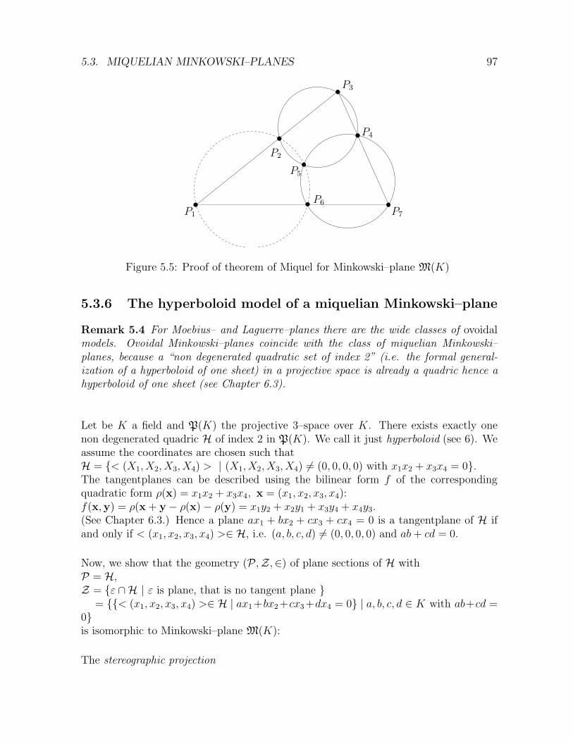
5.3. MIQUELIAN MINKOWSKI–PLANES 97
P1
P2
P3
P4
P5
P6
P7
Figure 5.5: Proof of theorem of Miquel for Minkowski–plane M(K)
5.3.6 The hyperboloid model of a miquelian Minkowski–plane
Remark 5.4 For Moebius– and Laguerre–planes there are the wide classes of ovoidalmodels. Ovoidal Minkowski–planes coincide with the class of miquelian Minkowski–planes, because a “non degenerated quadratic set of index 2” (i.e. the formal general-ization of a hyperboloid of one sheet) in a projective space is already a quadric hence ahyperboloid of one sheet (see Chapter 6.3).
Let be K a field and P(K) the projective 3–space over K. There exists exactly onenon degenerated quadric H of index 2 in P(K). We call it just hyperboloid (see 6). Weassume the coordinates are chosen such thatH = {< (X1, X2, X3, X4) > | (X1, X2, X3, X4) 6= (0, 0, 0, 0) with x1x2 + x3x4 = 0}.The tangentplanes can be described using the bilinear form f of the correspondingquadratic form ρ(x) = x1x2 + x3x4, x = (x1, x2, x3, x4):f(x,y) = ρ(x + y − ρ(x)− ρ(y) = x1y2 + x2y1 + x3y4 + x4y3.(See Chapter 6.3.) Hence a plane ax1 + bx2 + cx3 + cx4 = 0 is a tangentplane of H ifand only if < (x1, x2, x3, x4) >∈ H, i.e. (a, b, c, d) 6= (0, 0, 0, 0) and ab+ cd = 0.
Now, we show that the geometry (P,Z,∈) of plane sections of H withP = H,Z = {ε ∩H | ε is plane, that is no tangent plane }
= {{< (x1, x2, x3, x4) >∈ H | ax1+bx2+cx3+dx4 = 0} | a, b, c, d ∈ K with ab+cd =0}is isomorphic to Minkowski–plane M(K):
The stereographic projection
98 CHAPTER 5. MINKOWSKI–PLANES
ψ :
P → (K ∪ {∞})2
< (0, 0, 1, 0) > → (∞,∞)< (1, 0, u, 0) > → (∞,−u)< (0, 1, v, 0) > → (−v,∞)
< (x, y,−xy, 1) > → (x, y)maps the cycle with equation ax1 + bx2 + dx4 = 0 (i.e. c = 0!) onto{(x, y) ∈ K2 | y = −ax+d
b} ∪ {(∞,∞)}
and the cycle with equation ax1 + bx2 + cx3 + dx4 = 0, c 6= 0 onto{(x, y) ∈ K2 | y = −ax+d
cx−b, x 6= b
c} ∪ {(∞, a
c), ( b
c,∞)}.
(In any case the constraint ab+ cd 6= 0 is valid.)Obviously ψ is an isomorphism from (P,Z,∈) onto M(K).
5.3.7 The bundle theorem for Minkowski–planes
Similar to Moebius– and Laguerre–planes we have a Bundle Theorem. But for Minkowski–planes there are no non miquelian ovoidal Minkowski–planes.
Theorem 5.19 (Bundle Theorem) For a miquelian Minkowski–plane M the follow-ing statement holds:Let be A1, A2, A3, A4, B1, B2, B3, B4 eight pairwise non parallel points. If 5 of the sixquadruples Qij := {Ai, Bi, Aj , Bj}, i < j, are concyclical on at least 4 cycles kij thenthis is true for the last quadruple, too (see Theorem 3.25).
Proof: Analogously to the Bundle Theorem for ovoidal Moebius–planes (Theorem3.25).
Unlike the Moebius and the Laguerre case the Bundle Theorem for Minkowski–planesis equivalent to the Theorem of Miquel.
Result 5.20 (KAHN, [KH’80]) A Minkowski–plane is miquelian if and only if theBundle Theorem (Theorem 5.19) holds.
5.4 Minkowski–planes over TITS–nearfields
5.4.1 The incidence structure M(K, f)
Looking for further examples of Minkowski–planes we shall consider the close connectionbetween a miquelian Minkowski–plane M(K) and the group PGL(2, K). There are alot of sharply 3-transitive operating permutation groups which are no PGLs. They areall defined via TITS–nearfields (see Chapter 7). One may consider such a group as ageneralization of the group of fractional linear mappings.
5.4. MINKOWSKI–PLANES OVER TITS–NEARFIELDS 99
Let be (K,+, ·, f) a planar TITS–nearfield (see 7) and ∞ /∈ K. We define:a · ∞ = ∞, b+∞ = ∞ for a, b ∈ K, a 6= 0, andf : K ∪ {∞} → K ∪ {∞} with f(x) = f(x) for x ∈ K \ {0}, f(∞) = 0, f(0) = ∞.Hence the set of permutationsΠ(K, f) := {x→ ax+ b | a, b ∈ K, a 6= 0} ∪ {x→ af(x− b) + c | a, b, c ∈ K, a 6= 0}is a group which operates sharply 3-transitive on K ∪ {∞} (see 7).Herewith we defineP := (K ∪ {∞})2, the set of pointsZ := {{(x, y) ∈ P | y = π(x)} | π ∈ Π(K, f)} the set of cycles,(x1, y1) ‖+ (x2, y2) iff x1 = x2, (x1, y1) ‖− (x2, y2) iff y1 = y2, andM(K, f) := (P,Z; ‖+, ‖−,∈).The proof that M(K, f) is a Minkowski–plane will be performed in the same way as forthe miquelian examples.
5.4.2 Automorphisms of M(K, f). M(K, f) is a Minkowski–plane
Alike the miquelian case it is easy to find automorphisms of the incidence structure(P,Z,∈) of M(K, f), which we call automorphisms of M(K, f).
Lemma 5.21 Any of the following permutations of P is an automorphism of M(K, f).
a) (x, y) → (y, x)
b) (x, y) → (α(x), β(y)), with α, β ∈ Π(K, f)
c) (x, y) → (κ(x), κ(y)), where κ(∞) = ∞ and the restriction of κ onto K is anautomorphism of the TITS-nearfield (K,+, ·, f) (see 7).
The proof results from the fact that Π(K, f) is a group and the permutability of anautomorphism of TITS–nearfield (K,+, ·, f) with function f .
From the 3-transitivity of Π(K, f) we get
Lemma 5.22 The automorphism group of M(K, f) operates transitivelya) on the triples of points which are pairwise not parallel andb) on the set of cycles.
Herewith we proof the following theorem.
Theorem 5.23 M(K, f) is a Minkowski–plane.
Proof: Obviously the relations ‖+ and ‖− are equivalence relations on P. Because ofthe planarity of the nearfield K the residue A(∞,∞) (see Theorem 5.4) is an affine plane.And from Lemma 5.22 we get: Any residue is an affine plane. Theorem 5.4 completesthe proof. 2
100 CHAPTER 5. MINKOWSKI–PLANES
Remark 5.5 One easily checks that the list of automorphisms given in Section 5.3.2is valid for M(K, f) if one replaces 1
xand 1
yby f(x) and f(y), respectively. Even
their geometrical meaning can be adopted literally. The essential difference between amiquelian Minkowski–plane and one over a TITS–nearfield is the following one: Becauseof automorphisms (2) and (3) (of the list mentioned above) and the commutativity inthe miquelian case any mapping (x, y) → (xs, ys), s ∈ K{0} is an automorphism, too.This not true for a Minkowski–plane over a proper TITS-nearfield.
Alike the miquelian case (see Theorem 5.10) we get
Result 5.24 (Wefelscheid, [WE’77]) The automorphisms of Lemma 5.21 generatethe full group of automorphisms of Minkowski–plane M(K, f).
5.5 Minkowski–planes and sets of permutations
Another idea to find further examples of Minkowski–planes exploits the connection ofan arbitrary Minkowski–plane and sharply 3-transitive operating sets of permutations.
5.5.1 Description of a Minkowski–plane by permutation sets
Let be M = (P,Z; ‖+, ‖−,∈) a Minkowski–plane, z0 a cycle, E−0 a generator (∈ E−)
and K ∪ {∞},∞ /∈ K, the set of points of E−0 such that ∞ /∈ E−
0 ∩ z0. With help ofE−
0 and z0 we define a bijection ψ from P onto (K ∪ {∞})2:
ψ :
{
P → (K ∪ {∞})2
P → (P+ ∩ E−0 , (P− ∩ z0)+ ∩ E−
0 )Identifying P and ψ(P) we getP = (K ∪ {∞})2 and(x1, y1) ‖+ (x2, y2) iff x1 = x2, (x1, y1) ‖− (x2, y2) iff y1 = y2.To any cycle z we assign a permutation πz of K ∪ {∞}:
πz :
{
K ∪ {∞} → K ∪ {∞}
x → ((x+ ∩ z)− ∩ z0)+ ∩ E−0
.
Because of axiom (C3) the permutation set Π(z0, E−0 ) := {πz | z ∈ Z} operates sharply
3–transitive on K ∪ {∞}.
Remark 5.6 If M is a Minkowski–plane M(K, f) over a TITS–nearfield, z0 the cycley = x and E−
0 the generator y = 0 we get Π(z0, E−0 ) = Π(K, f). Especiellay Π(z0, E
−0 ) is
a group. In Section 5.5.2 we shall recognize that this property is typical for Minkowski–planes over TITS-nearfields. (Notice: Till now (1985) it is unknown if any sharply3–transitive permutation group can be described over a TITS–nearfield. For permuta-tiongroups coming with Minkowski–planes this is always true, see Section 5.5.2.) Hence
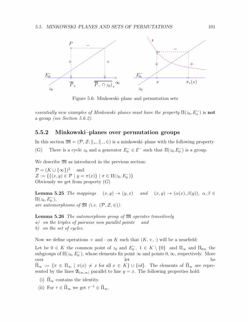
5.5. MINKOWSKI–PLANES AND SETS OF PERMUTATIONS 101
zP
E−0E−
0
z0z0
x πz(x)P+ P− ∩ z0)+∞
+ +++
−−
Figure 5.6: Minkowski–plane and permutation sets
essentially new examples of Minkowski–planes must have the property Π(z0, E−o ) is not
a group (see Section 5.6.2).
5.5.2 Minkowski–planes over permutation groups
In this section M = (P,Z; ‖+, ‖−,∈) is a minkowski–plane with the following property
(G) There is a cycle z0 and a generator E−0 ∈ E− such that Π(z0.E
−0 ) is a group.
We describe M as introduced in the previous section:
P = (K ∪ {∞})2 andZ := {{(x, y) ∈ P | y = π(x)} | π ∈ Π(z0, E
−0 )}
Obviously we get from property (G)
Lemma 5.25 The mappings (x, y) → (y, x) and (x, y) → (α(x), β(y)), α, β ∈Π(z0, E
−0 ),
are automorphisms of M (i.e. (P,Z,∈)).
Lemma 5.26 The automorphism group of M operates transitivelya) on the triples of pairwise non parallel points andb) on the set of cycles.
Now we define operations + and · on K such that (K,+, ·) will be a nearfield:
Let be 0 ∈ K the common point of z0 and E−0 , 1 ∈ K \ {0} and Π∞ and Π0∞ the
subgroups of Π(z0, E−0 ), whose elements fix point ∞ and points 0,∞, respectively. More
over let beΠ∞ := {π ∈ Π∞ | π(x) 6= x for all x ∈ K} ∪ {id}. The elements of Π∞ are repre-sented by the lines A(∞,∞) parallel to line y = x. The following properties hold:
(i) Π∞ contains the identity.
(ii) For τ ∈ Π∞ we get τ−1 ∈ Π∞.
102 CHAPTER 5. MINKOWSKI–PLANES
(iii) For τ1, τ2 ∈ Π∞ we get τ1τ2 ∈ Π∞.
(iv) For τ1, τ2 ∈ Π∞ and x0 ∈ K we get from τ1(x0) = τ2(x0) the equation τ1 = τ2.
(For the proof of these statements prove (iv) before (iii).)
Hence Π∞ is a permutation group of K which operates sharply transitive (regular).
Below let be τa ∈ (πb, b ∈ K \ {0}) the unique mapping out of Π∞ ( of Π0∞) withτ(0) = a (πb(1) = b). On the set K we define the operations + and · , respectively, by
+ :
{
K2 → K(a, b) → τa(b)
· :
K2 → K(a, b) → 0, if a = 0 or b = 0(a, b) → πa(b) if a 6= 0 and b 6= 0.
(K,+, ·) has the following properties:
(F1): (K,+) is a group (0 is the neutral element).
(F2): (K \ {0}, ·) is a group (1 is the neutral element).
Because of a(b+ c) = πaτb(c) = πaτbπ−1a πa(c) = τπa(b)πa(c) = τabπa(c) = ab+ ac
for any a, b, c ∈ K we get
(F3): a(b+ c) = ab+ ac for any a, b, c ∈ K.
(F4): 0a = 0 for any a ∈ K.
An algebraic structure (K,+, ·) with properties (F1) − −(F4) is called nearfield (s.Chapter 7). For a nearfield (K,+, ·) group (K,+) is commutative, −1 is an element ofthe center and equation x2 = 1 has only the solutions 1 and −1 (s. Section 7.1).
Because {x → ax + b | a, b,∈ K, a 6= 0} operates sharply 2-transitive on K, like Π∞
does, and is a subgroup of the restriction of Π∞ on K we get
Π∞ =
{
∞ → ∞x → ax+ b
| a, b ∈ K, a 6= 0
}
, Π∞ =
{
∞ → ∞x → x+ b
| b ∈ K
}
and
Π0∞ =
{
∞ → ∞x → ax
| a ∈ K, a 6= 0
}
.
Obviously the lines of residue A(∞,∞) are represented by equations y = ax+b and x = c.From the parallel axiom of an affine plane we find that any line y = ax+ b with a 6= 1intersects line y = x and nearfiled (K,+, ·) has the following property:
(p) For any a, b ∈ K with a 6= 1 equation ax− x = b has a solution in K.
Hence (K,+, ·) is a planar nearfield (s. Section 7.3. In order to verify property (t) be-low, we consider:If f ∈ Π(z0, E
−0 ) and f(1) = 1, f(0) = ∞, f(∞) = 0 then
f(ab) = f(πa(b)) = fπaf−1f(b) = πf(a)f(b) = f(a)f(b) for any a, b ∈ K \ {0}.
For a nearfield equation x2 = 1 has only the two solutions 1 and −1. From f(ab) =
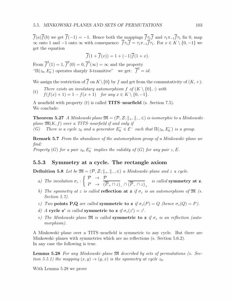
5.5. MINKOWSKI–PLANES AND SETS OF PERMUTATIONS 103
f(a)f(b) we get f(−1) = −1. Hence both the mappings fτ1f and τ1π−1fτ1 fix 0, map∞ onto 1 and −1 onto ∞ with consequence: fτ1f = τ1π−1fτ1. For x ∈ K \ {0,−1} weget the equation
f(1 + f(x)) = 1 + (−1)f(1 + x).
From f2(1) = 1, f
2(0) = 0, f
2(∞) = ∞ and the property
“Π(z0, E−0 ) operates sharply 3-transitive” we get: f
2= id.
We assign the restriction of f on K \{0} by f and get from the commutativity of (K,+):
(t)There exists an involutary automorphism f of (K \ {0}, ·) withf(f(x) + 1) = 1− f(x+ 1) for any x ∈ K \ {0,−1}.
A nearfield with property (t) is called TITS–nearfield (s. Section 7.5).We conclude:
Theorem 5.27 A Minkowski planeM = (P,Z; ‖+, ‖−,∈) is isomorphic to a Minkowski–plane M(K, f) over a TITS–nearfield if and only if(G) There is a cycle z0 and a generator E−
0 ∈ E− such that Π(z0, E−0 ) is a group.
Remark 5.7 From the abundance of the automorphism group of a Minkowski–plane wefind:Property (G) for a pair z0, E
−0 implies the validity of (G) for any pair z, E.
5.5.3 Symmetry at a cycle. The rectangle axiom
Definition 5.8 Let be M = (P,Z; ‖+, ‖−,∈) a Minkowski–plane and z a cycle.
a) The involution σz :
{
P → P
P → (P+ ∩ z)− ∩ (P− ∩ z)+is called symmetry at z.
b) The symmetry at z is called reflection at z if σz is an automorphism of M (s.Section 5.7).
c) Two points P,Q are called symmetric to z if σz(P ) = Q (hence σz(Q) = P ).
d) A cycle z’ is called symmetric to z if σz(z′) = z′.
e) The Minkowski–plane M is called symmetric to z if σz is an reflection (auto-morphism).
A Minkowski–plane over a TITS–nearfield is symmetric to any cycle. But there areMinkowski–planes with symmetries which are no reflections (s. Section 5.6.2).In any case the following is true.
Lemma 5.28 For any Minkowski–plane M described by sets of permutations (s. Sec-tion 5.5.1) the mapping (x, y) → (y, x) is the symmetry at cycle z0.
With Lemma 5.28 we prove
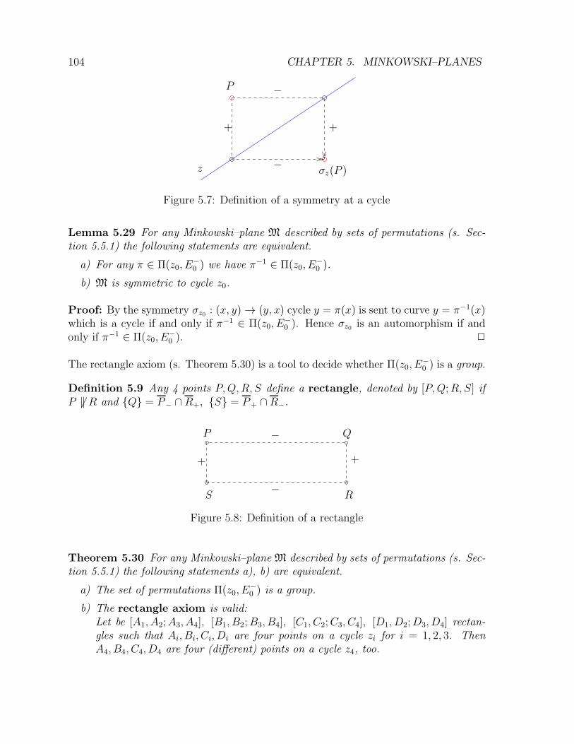
104 CHAPTER 5. MINKOWSKI–PLANES
P
z σz(P )
++
−
−
Figure 5.7: Definition of a symmetry at a cycle
Lemma 5.29 For any Minkowski–plane M described by sets of permutations (s. Sec-tion 5.5.1) the following statements are equivalent.
a) For any π ∈ Π(z0, E−0 ) we have π−1 ∈ Π(z0, E
−0 ).
b) M is symmetric to cycle z0.
Proof: By the symmetry σz0 : (x, y) → (y, x) cycle y = π(x) is sent to curve y = π−1(x)which is a cycle if and only if π−1 ∈ Π(z0, E
−0 ). Hence σz0 is an automorphism if and
only if π−1 ∈ Π(z0, E−0 ). 2
The rectangle axiom (s. Theorem 5.30) is a tool to decide whether Π(z0, E−0 ) is a group.
Definition 5.9 Any 4 points P,Q,R, S define a rectangle, denoted by [P,Q;R, S] ifP 6‖ R and {Q} = P− ∩ R+, {S} = P+ ∩R−.
P Q
RS
++
−
−
Figure 5.8: Definition of a rectangle
Theorem 5.30 For any Minkowski–plane M described by sets of permutations (s. Sec-tion 5.5.1) the following statements a), b) are equivalent.
a) The set of permutations Π(z0, E−0 ) is a group.
b) The rectangle axiom is valid:Let be [A1, A2;A3, A4], [B1, B2;B3, B4], [C1, C2;C3, C4], [D1, D2;D3, D4] rectan-gles such that Ai, Bi, Ci, Di are four points on a cycle zi for i = 1, 2, 3. ThenA4, B4, C4, D4 are four (different) points on a cycle z4, too.
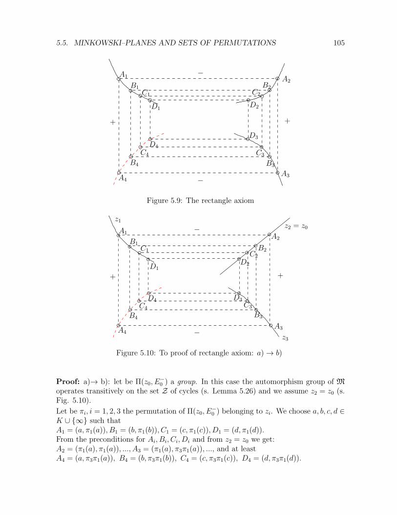
5.5. MINKOWSKI–PLANES AND SETS OF PERMUTATIONS 105
A1
B1C1
D1
A2B2
C2
D2
A3
B3
C3
D3
A4
B4
C4
D4
+ +
−
−
Figure 5.9: The rectangle axiom
A1
B1C1
D1
A2
B2C2
D2
A3
B3
C3
D3
A4
B4
C4
D4
z1
z3
z2 = z0
+ +
−
−
Figure 5.10: To proof of rectangle axiom: a) → b)
Proof: a)→ b): let be Π(z0, E−0 ) a group. In this case the automorphism group of M
operates transitively on the set Z of cycles (s. Lemma 5.26) and we assume z2 = z0 (s.Fig. 5.10).
Let be πi, i = 1, 2, 3 the permutation of Π(z0, E−0 ) belonging to zi. We choose a, b, c, d ∈
K ∪ {∞} such thatA1 = (a, π1(a)), B1 = (b, π1(b)), C1 = (c, π1(c)), D1 = (d, π1(d)).From the preconditions for Ai, Bi, Ci, Di and from z2 = z0 we get:A2 = (π1(a), π1(a)), ..., A3 = (π1(a), π3π1(a)), ..., and at leastA4 = (a, π3π1(a)), B4 = (b, π3π1(b)), C4 = (c, π3π1(c)), D4 = (d, π3π1(d)).
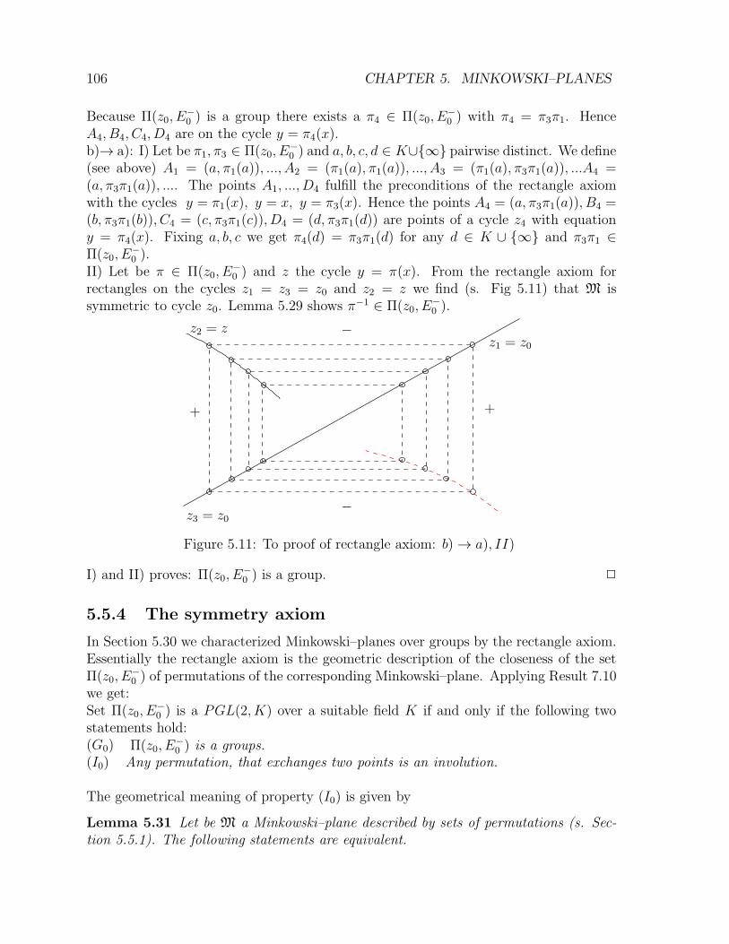
106 CHAPTER 5. MINKOWSKI–PLANES
Because Π(z0, E−0 ) is a group there exists a π4 ∈ Π(z0, E
−0 ) with π4 = π3π1. Hence
A4, B4, C4, D4 are on the cycle y = π4(x).b)→ a): I) Let be π1, π3 ∈ Π(z0, E
−0 ) and a, b, c, d ∈ K∪{∞} pairwise distinct. We define
(see above) A1 = (a, π1(a)), ..., A2 = (π1(a), π1(a)), ..., A3 = (π1(a), π3π1(a)), ...A4 =(a, π3π1(a)), .... The points A1, ..., D4 fulfill the preconditions of the rectangle axiomwith the cycles y = π1(x), y = x, y = π3(x). Hence the points A4 = (a, π3π1(a)), B4 =(b, π3π1(b)), C4 = (c, π3π1(c)), D4 = (d, π3π1(d)) are points of a cycle z4 with equationy = π4(x). Fixing a, b, c we get π4(d) = π3π1(d) for any d ∈ K ∪ {∞} and π3π1 ∈Π(z0, E
−0 ).
II) Let be π ∈ Π(z0, E−0 ) and z the cycle y = π(x). From the rectangle axiom for
rectangles on the cycles z1 = z3 = z0 and z2 = z we find (s. Fig 5.11) that M issymmetric to cycle z0. Lemma 5.29 shows π−1 ∈ Π(z0, E
−0 ).
z1 = z0
z3 = z0
z2 = z
+ +
−
−
Figure 5.11: To proof of rectangle axiom: b) → a), II)
I) and II) proves: Π(z0, E−0 ) is a group. 2
5.5.4 The symmetry axiom
In Section 5.30 we characterized Minkowski–planes over groups by the rectangle axiom.Essentially the rectangle axiom is the geometric description of the closeness of the setΠ(z0, E
−0 ) of permutations of the corresponding Minkowski–plane. Applying Result 7.10
we get:Set Π(z0, E
−0 ) is a PGL(2, K) over a suitable field K if and only if the following two
statements hold:(G0) Π(z0, E
−0 ) is a groups.
(I0) Any permutation, that exchanges two points is an involution.
The geometrical meaning of property (I0) is given by
Lemma 5.31 Let be M a Minkowski–plane described by sets of permutations (s. Sec-tion 5.5.1). The following statements are equivalent.
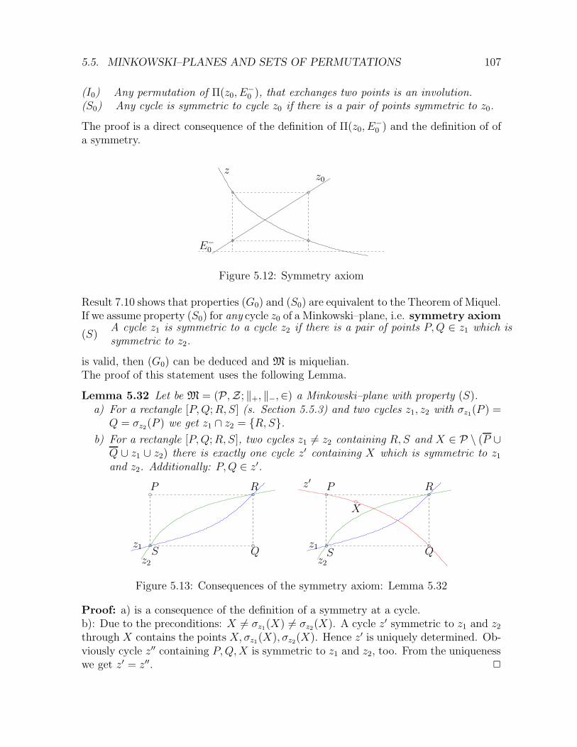
5.5. MINKOWSKI–PLANES AND SETS OF PERMUTATIONS 107
(I0) Any permutation of Π(z0, E−0 ), that exchanges two points is an involution.
(S0) Any cycle is symmetric to cycle z0 if there is a pair of points symmetric to z0.
The proof is a direct consequence of the definition of Π(z0, E−0 ) and the definition of of
a symmetry.
zz0
E−0
Figure 5.12: Symmetry axiom
Result 7.10 shows that properties (G0) and (S0) are equivalent to the Theorem of Miquel.If we assume property (S0) for any cycle z0 of a Minkowski–plane, i.e. symmetry axiom
(S)A cycle z1 is symmetric to a cycle z2 if there is a pair of points P,Q ∈ z1 which issymmetric to z2.
is valid, then (G0) can be deduced and M is miquelian.The proof of this statement uses the following Lemma.
Lemma 5.32 Let be M = (P,Z; ‖+, ‖−,∈) a Minkowski–plane with property (S).a) For a rectangle [P,Q;R, S] (s. Section 5.5.3) and two cycles z1, z2 with σz1(P ) =
Q = σz2(P ) we get z1 ∩ z2 = {R, S}.
b) For a rectangle [P,Q;R, S], two cycles z1 6= z2 containing R, S and X ∈ P \ (P ∪Q ∪ z1 ∪ z2) there is exactly one cycle z′ containing X which is symmetric to z1and z2. Additionally: P,Q ∈ z′.
z1z1
z2z2
z′ PP
RR
SS
X
Figure 5.13: Consequences of the symmetry axiom: Lemma 5.32
Proof: a) is a consequence of the definition of a symmetry at a cycle.b): Due to the preconditions: X 6= σz1(X) 6= σz2(X). A cycle z′ symmetric to z1 and z2through X contains the points X, σz1(X), σz2(X). Hence z′ is uniquely determined. Ob-viously cycle z′′ containing P,Q,X is symmetric to z1 and z2, too. From the uniquenesswe get z′ = z′′. 2
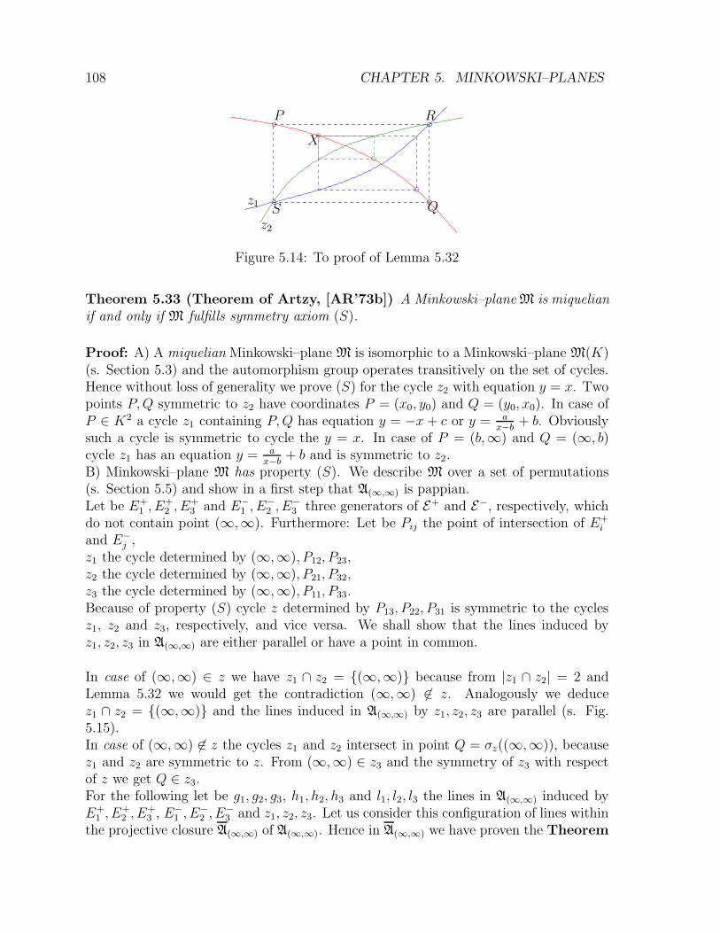
108 CHAPTER 5. MINKOWSKI–PLANES
z1
z2
P
Q
R
S
X
Figure 5.14: To proof of Lemma 5.32
Theorem 5.33 (Theorem of Artzy, [AR’73b]) A Minkowski–planeM is miquelianif and only if M fulfills symmetry axiom (S).
Proof: A) A miquelian Minkowski–plane M is isomorphic to a Minkowski–plane M(K)(s. Section 5.3) and the automorphism group operates transitively on the set of cycles.Hence without loss of generality we prove (S) for the cycle z2 with equation y = x. Twopoints P,Q symmetric to z2 have coordinates P = (x0, y0) and Q = (y0, x0). In case ofP ∈ K2 a cycle z1 containing P,Q has equation y = −x + c or y = a
x−b+ b. Obviously
such a cycle is symmetric to cycle the y = x. In case of P = (b,∞) and Q = (∞, b)cycle z1 has an equation y = a
x−b+ b and is symmetric to z2.
B) Minkowski–plane M has property (S). We describe M over a set of permutations(s. Section 5.5) and show in a first step that A(∞,∞) is pappian.Let be E+
1 , E+2 , E
+3 and E−
1 , E−2 , E
−3 three generators of E+ and E−, respectively, which
do not contain point (∞,∞). Furthermore: Let be Pij the point of intersection of E+i
and E−j ,
z1 the cycle determined by (∞,∞), P12, P23,z2 the cycle determined by (∞,∞), P21, P32,z3 the cycle determined by (∞,∞), P11, P33.Because of property (S) cycle z determined by P13, P22, P31 is symmetric to the cyclesz1, z2 and z3, respectively, and vice versa. We shall show that the lines induced byz1, z2, z3 in A(∞,∞) are either parallel or have a point in common.
In case of (∞,∞) ∈ z we have z1 ∩ z2 = {(∞,∞)} because from |z1 ∩ z2| = 2 andLemma 5.32 we would get the contradiction (∞,∞) 6∈ z. Analogously we deducez1 ∩ z2 = {(∞,∞)} and the lines induced in A(∞,∞) by z1, z2, z3 are parallel (s. Fig.5.15).In case of (∞,∞) 6∈ z the cycles z1 and z2 intersect in point Q = σz((∞,∞)), becausez1 and z2 are symmetric to z. From (∞,∞) ∈ z3 and the symmetry of z3 with respectof z we get Q ∈ z3.For the following let be g1, g2, g3, h1, h2, h3 and l1, l2, l3 the lines in A(∞,∞) induced byE+
1 , E+2 , E
+3 , E
−1 , E
−2 , E
−3 and z1, z2, z3. Let us consider this configuration of lines within
the projective closure A(∞,∞) of A(∞,∞). Hence in A(∞,∞) we have proven the Theorem
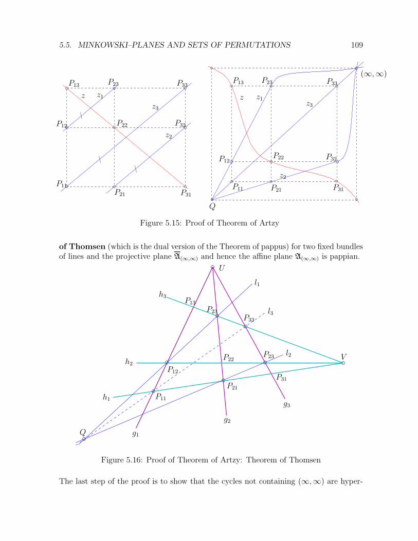
5.5. MINKOWSKI–PLANES AND SETS OF PERMUTATIONS 109
zz z1z1
z2
z2
z3z3
P11 P11
P12
P12
P13P13
P21P21
P22
P22
P23P23
P31P31
P32
P32
P33P33
(∞,∞)
Q
Figure 5.15: Proof of Theorem of Artzy
of Thomsen (which is the dual version of the Theorem of pappus) for two fixed bundlesof lines and the projective plane A(∞,∞) and hence the affine plane A(∞,∞) is pappian.
g1
g2
g3h1
h2
h3
l1
l2
l3
P11
P12
P13
P21
P22P23
P23
P31
P33
Q
U
V
Figure 5.16: Proof of Theorem of Artzy: Theorem of Thomsen
The last step of the proof is to show that the cycles not containing (∞,∞) are hyper-
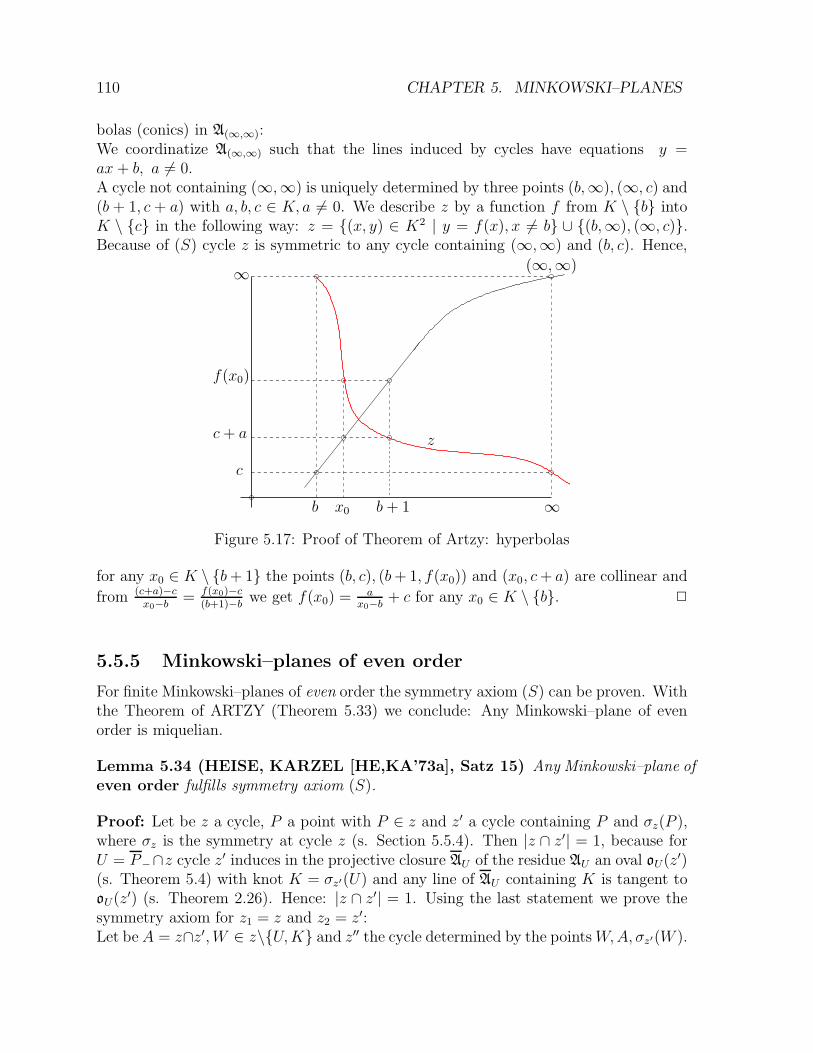
110 CHAPTER 5. MINKOWSKI–PLANES
bolas (conics) in A(∞,∞):We coordinatize A(∞,∞) such that the lines induced by cycles have equations y =ax+ b, a 6= 0.A cycle not containing (∞,∞) is uniquely determined by three points (b,∞), (∞, c) and(b + 1, c + a) with a, b, c ∈ K, a 6= 0. We describe z by a function f from K \ {b} intoK \ {c} in the following way: z = {(x, y) ∈ K2 | y = f(x), x 6= b} ∪ {(b,∞), (∞, c)}.Because of (S) cycle z is symmetric to any cycle containing (∞,∞) and (b, c). Hence,
z
∞
∞(∞,∞)
f(x0)
c+ a
c
b x0 b+ 1
Figure 5.17: Proof of Theorem of Artzy: hyperbolas
for any x0 ∈ K \ {b+ 1} the points (b, c), (b+ 1, f(x0)) and (x0, c+ a) are collinear and
from (c+a)−cx0−b
= f(x0)−c(b+1)−b
we get f(x0) =a
x0−b+ c for any x0 ∈ K \ {b}. 2
5.5.5 Minkowski–planes of even order
For finite Minkowski–planes of even order the symmetry axiom (S) can be proven. Withthe Theorem of ARTZY (Theorem 5.33) we conclude: Any Minkowski–plane of evenorder is miquelian.
Lemma 5.34 (HEISE, KARZEL [HE,KA’73a], Satz 15) Any Minkowski–plane ofeven order fulfills symmetry axiom (S).
Proof: Let be z a cycle, P a point with P ∈ z and z′ a cycle containing P and σz(P ),where σz is the symmetry at cycle z (s. Section 5.5.4). Then |z ∩ z′| = 1, because forU = P−∩z cycle z
′ induces in the projective closure AU of the residue AU an oval oU(z′)
(s. Theorem 5.4) with knot K = σz′(U) and any line of AU containing K is tangent tooU(z
′) (s. Theorem 2.26). Hence: |z ∩ z′| = 1. Using the last statement we prove thesymmetry axiom for z1 = z and z2 = z′:Let be A = z∩z′,W ∈ z\{U,K} and z′′ the cycle determined by the pointsW,A, σz′(W ).
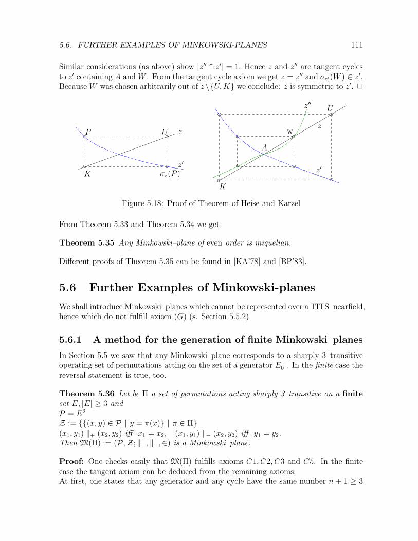
5.6. FURTHER EXAMPLES OF MINKOWSKI-PLANES 111
Similar considerations (as above) show |z′′ ∩ z′| = 1. Hence z and z′′ are tangent cyclesto z′ containing A andW . From the tangent cycle axiom we get z = z′′ and σz′(W ) ∈ z′.Because W was chosen arbitrarily out of z\{U,K} we conclude: z is symmetric to z′. 2
Wz
z
U
U
K
K
A
P
z′z′
z′′
σz(P )
Figure 5.18: Proof of Theorem of Heise and Karzel
From Theorem 5.33 and Theorem 5.34 we get
Theorem 5.35 Any Minkowski–plane of even order is miquelian.
Different proofs of Theorem 5.35 can be found in [KA’78] and [BP’83].
5.6 Further Examples of Minkowski-planes
We shall introduce Minkowski–planes which cannot be represented over a TITS–nearfield,hence which do not fulfill axiom (G) (s. Section 5.5.2).
5.6.1 A method for the generation of finite Minkowski–planes
In Section 5.5 we saw that any Minkowski–plane corresponds to a sharply 3–transitiveoperating set of permutations acting on the set of a generator E−
0 . In the finite case thereversal statement is true, too.
Theorem 5.36 Let be Π a set of permutations acting sharply 3–transitive on a finiteset E, |E| ≥ 3 andP = E2
Z := {{(x, y) ∈ P | y = π(x)} | π ∈ Π}(x1, y1) ‖+ (x2, y2) iff x1 = x2, (x1, y1) ‖− (x2, y2) iff y1 = y2.Then M(Π) := (P,Z; ‖+, ‖−,∈) is a Minkowski–plane.
Proof: One checks easily that M(Π) fulfills axioms C1, C2, C3 and C5. In the finitecase the tangent axiom can be deduced from the remaining axioms:At first, one states that any generator and any cycle have the same number n + 1 ≥ 3
112 CHAPTER 5. MINKOWSKI–PLANES
of points and that for two non parallel points there are exactly n− 1 cycles containingthese two points.For the following let be P, P ′ and z defined as in axiom C4. Then z contains exactlyn− 2 points different from P and not parallel to P ′. Because of C3 exactly n− 2 cyclesthrough P and P ′ meet z at 2 points. On the other hand we know that there are n− 1cycles through P and P ′. Hence there is exactly one cycle through P and P ′ which istangent to z at point P . 2
Theorem 5.36 will be used in the next section.
5.6.2 Finite examples which do not fulfill (G)
Let be (K,+, ·) the field with pn elements with p > 2, 3 ≤ n ∈ IN, γ the automorphismx→ xp and Q the set of squares of K. Π is the following subset of the set of semi-linearmappings (s. Section 1.2.7)
Π = {x→ ax+bcx+d
| a, b, c, d ∈ K, ad−bc ∈ Q}∪{x → aγ(x)+bcγ(x)+d
| a, b, c, d ∈ K, ad−bc 6∈ Q}.
(Π operates on K ∪ {∞}.)For k0 ∈ K \Q and α0 : x→ k0γ(x) we have Π = PSL(2, pn) ∪ PSL(2, pn)α0.(Replacing γ by the identity we get Π = PGL(2, pn). For n = 2 set Π would be thesharply 3-transitive operating group over the nearfield FK(p2) (s. Section 7.5).)
Lemma 5.37 (PERCSY [PE’81]) Π operates sharply 3–transitive on K ∪ {∞}.
Proof: Group PSL(2, pn) and hence Π operates 2–transitively.Π0∞ := {x → ax | 0 6= a ∈ Q} ∪ {x → bγ(x) | b 6∈ Q} is the subset of Π which fixes0 and ∞ and operates sharply transitive (regular) on K \ {0}. Hence Π itself operatessharply 3–transitive. 2
Because of Theorem 5.36 there exists a corresponding Minkowski–plane which we ab-breviate by M(Π, pn). Its automorphism group is rather large:
Lemma 5.38 For the Minkowski–plane M(Π, pn) the following mappings are automor-phisms (of the incidence structure (P,Z,∈)):(x, y) → (y, x) and (x, y) → (τ1(x), τ2(y)), τ1, τ2 ∈ PSL(2, pn).
Proof: The proof results from the two properties:(1) PSL(2, pn) is a group, (2) PSL(2, pn)α0 = α0PSL(2, p
n). 2
Remark 5.8 In case of pn ≡ 1 mod 4 element −1 is a square and the mapping x→ −xis contained in PSL(2, pn). Hence the reflections at generators (x, y) → (−x, y) and(x, y) → (x,−y) are automorphisms of M(Π, pn).
5.6. FURTHER EXAMPLES OF MINKOWSKI-PLANES 113
5.6.3 Real examples, which do not fulfill (G)
We start from the classical real Minkowski–plane, i.e. P = (IR ∪ {∞})2, and replacethe cycles Z0 := {{(x, y) ∈ P | y = π(x)} | π ∈ PGL(2, IR)} by the system Z1(f) andZ2(f), respectively, of curves.
Definition 5.10 Let be f a monotone increasing bijection of IR onto itself with f(0) =0, f(1) = 1 and f the bijection of IR∪{∞} with f(∞) = ∞ and f(x) = f(x) for x ∈ IR.Using Π := PSL(2, IR) ∪ PSL(2, IR) · (−f) we defineZ1(f) := {{(x, y) ∈ P | y = π(x)} | π ∈ Π}
= {{(x, y) ∈ IR2 | y = ax+ b} ∪ {(∞,∞)} | a, b ∈ IR, a > 0}
∪ {{(x, y) ∈ IR2 | y = af(x) + b} ∪ {(∞,∞)} | a, b ∈ IR, a < 0}
∪ {{(x, y) ∈ IR2 | y = a
x−b+ c, x 6= b} ∪ {(b,∞), (∞, c)} | a, b, c ∈ IR, a < 0}
∪{{(x, y) ∈ IR2 | y = a
f(x)−f(b)+c, x 6= b}∪{(b,∞), (∞, c)} | a, b, c ∈ IR, a > 0}
Alike the classical model we define M1(f) := (P,Z1(f),∈, ‖+, ‖−).It is easy to find automorphisms of M1(f):
Lemma 5.39 Any mapping (x, y) → (x, τ(y)), with τ ∈ PSL(2, IR), is an automor-phism of M1(f).
The proof is based on the fact that PSL(2, IR) is a group.
With help of Lemma 5.39 we prove the following theorem.
Theorem 5.40 (SCHENKEL, [SC’80]) M1(f) is a Minkowski–plane.
Proof: Because of Lemma 5.39 it is sufficient to prove that the residue A(x0,∞) at anypoint (x0,∞) is an affine plane. In case of x0 = ∞ the prove is obvious.In case of x0 = b 6= ∞ one maps A(x0,∞) by (x, y) → (− 1
x−b, y) onto IR
2. The imagesof the curves will be described by y = ax + b, a > 0 and y = ah(x) + b, a < 0 andx = c, y = d, respectively, where h is a monotone increasing bijection of IR. Such anincidence structure is (like the case A(∞,∞)) an affine plane. 2
Remark 5.9 a) M1(f) is miquelian if f(x) = x.
b) In non miquelian case any residue of M1(f) is a non desarguesian affine plane.
c) Topological properties were explored by Schenkel in [SC’80].
d) In case of f 6= identity the Minkowski–plane M1(f) does not fulfill axiom (G).
Definition 5.11 Let be g(x) :=
{ 1xm for x > 0
− 1|x|n
for x < 0,with 0 < m, n ∈ IR
fixed.
114 CHAPTER 5. MINKOWSKI–PLANES
Definition 5.12 Z2(g) := {{(x, y) ∈ IR2 | y = ax+ b} ∪ {(∞,∞)} | a, b ∈ IR, a 6= 0}
∪{{(x, y) ∈ IR2 | y = ag(x−b)+c, x 6= b}∪{(b,∞), (∞, c)} | a, b, c ∈ IR, a 6= 0}
Analogously we define M2(g) := (P,Z2(g),∈, ‖+, ‖−).
Result 5.41 (HARTMANN [HA’81a]) M2(g) is a Minkowski–plane.
Remark 5.10 a) MF2(g) is miquelian if and only if m = n = 1, i.e. g(x) = 1x.
b) In non miquelian case M2(g) does not fulfill axiom (G).
c) In [SC’80] Schenkel discussed these examples from a topological aspect.
5.7 Automorphisms of Minkowski–planes
We repeat the definition of an automorphism of a Minkowski–plane:
Definition 5.13 Let be M = (P,Z; ‖+, ‖−,∈) a Minkowski–plane. Any automorphismof the incidence Structure (P,Z,∈) is called automorphism of the Minkowski–plane.
There are automorphisms of a Minkowski–plane with special meanings:
Definition 5.14 Any automorphism of a Minkowski–plane M = (P,Z; ‖+, ‖−,∈)
a) that fixes two non parallel points P,Q and any cycle through P,Q is called dilata-tion at P,Q.Denotation of the group of such dilatations: ∆(P,Q).
b) that fixes two generators E+1 , E
+2 ∈ E+ (E−
1 , E−2 ∈ E−) pointwise is called dilata-
tion at E+1 , E
+2 (dilatation at E−
1 , E−2 ).
Denotation of the group of such dilatations: ∆(E+1 , E
+2 ) and ∆(E−
1 , E−2 ).
c) that fixes exactly one generator E+ ∈ E+ or P ( E+ ∈ E+ or P) pointwise is calledtranslation with axis E+ (E−).Denotation of the group of such translations: T (E+) and T (E−).
The following is true:
Lemma 5.42 a) Any δ ∈ ∆(P,Q) induces a dilatation in AP and AQ at a point([HA’82b], 2.1).
b) Any δ ∈ ∆(E+1 , E
+2 ) induces in any AP with P ∈ E+
1 ∪ E+2 a dilatation at a line.
(Analogously for ∆(E−1 , E
−2 ).)
c) Any τ ∈ T (E+) induces in any AP with P ∈ E+ a translation. (Analogously forT (E−).)
5.7. AUTOMORPHISMS OF MINKOWSKI–PLANES 115
Definition 5.15 a) A group ∆(P,Q) is called circular transitive if its restrictiononto AP (or AQ) is linear transitive.
b) A group ∆(E+1 , E
+2 ) or ∆(E−
1 , E−2 ) or T (E+) or T (E−), respectively, is called
circular transitive if its restriction on a residue AP of a fixed point P is lineartransitive.
For involutions we give the following definition:
Definition 5.16 An involutorial automorphism of a Minkowski–plane M = (P,Z; ‖+, ‖−,∈)
a) that fixes exactly one rectangle [P,Q;R, S] (s. Section 5.5.3) pointwise is calledreflection at rectangle [P,Q;R, S].
b) that fixes a cycle z pointwise is called reflection at cycle z.
c) that fixes a generator E pointwise is called reflection at generator E.
The next lemma clarifies the connection between reflections and involutorial dilatations.
Lemma 5.43 a) A reflection at a rectangle [P,Q;R, S] is a dilatation at P,R andQ, S.
b) An involutorial dilatation at two (non parallel) points P,R is a reflection at rect-angle [P,Q;R, S] with Q = P− ∩R+ and S = P+ ∩ R−.
c) An automorphism of a Minkowski–plane that fixes a cycle pointwise is the identityor the (unique) reflection at z.
Proof: a) Reflection σ at rectangle [P,Q;R, S] induces in residue AP an involutorialcollineation σ with single fixpoint R. From [HU,PI’73], pages 91,92 we know that σ is areflection (involutorial dilatation) at point R. Hence σ is a reflection at the points P,R.Analogously: σ is a reflection at the points Q, S, too.b) Let be δ an involutorial dilatation at P,R. Then points P,Q with {Q} := P− ∩ R+
and {S} := P+ ∩ R− are the sole further fixpoints of δ. Hence δ is the reflection atrectangle [P,Q;R, S].c) Let be ψ 6= id an automorphism of a Minkowski–plane which fixes a cycle pointwise.ψ exchanges E+ and E−. Otherwise, ψ would induce a central collineation with twocenters in the projective closure AP , P ∈ z of AP . One easily checks that ψ is thesymmetry at cycle z (s. Section 5.5.3) and hence the reflection at z. 2
Below we assemble some properties considering transitivity and reflections of Minkowski–planes over TITS–nearfields and miquelian Minkowski–planes, respectively.
Lemma 5.44 Let be M = (P,Z; ‖+, ‖−,∈) a Minkowski–plane over a TITS–nearfield.Then
116 CHAPTER 5. MINKOWSKI–PLANES
a) any group ∆(E+1 , E
+2 ) and ∆(E−
1 , E−2 ), respectively, of dilatations at two genera-
tors is circular transitive.
b) any group T (E+) and T (E−), respectively, of translations is circular transitive.
c) for any cycle there is a reflection.
d) for any three generators E+0 , E
+1 , E
+2 ∈ E+ (E−
0 , E−1 , E
−2 ∈ E−) there is exactly one
reflection at E+0 (E−
0 ) which exchanges E+1 with E+
2 (E−1 with E−
2 ).
e) in case of characteristic 6= 2 for any rectangle there is exactly one reflection.
Lemma 5.45 A miquelian Minkowski–plane M additionally fulfills:f) Any group ∆(P,Q) of dilatations at two points is circular transitive.
The proofs of these statements are performed easily with help of the automorphisms ofa Minkowski–plane M(K, f) and M(K), respectively, (s. Lemma 5.25 and Lemma 5.8).The following results show which properties are typical for Minkowski–planes over TITS–nearfields.
Result 5.46 (ARTZY [AR’77], PERCSY [PE’79]) For a Minkowski–plane M thefollowing statements are equivalent:
a) M can be described over a TITS–nearfield (s. Section 5.4).
b) Any group ∆(E+1 , E
+2 ) of dilatations is circular transitive.
c) Any group ∆(E−1 , E
−2 ) of dilatations is circular transitive.
Properties b) and c) can be weakened (s. [HA’82a]).
Result 5.47 (PERCSY [PE’81], HARTMANN [HA’81b]) A finite Minkowski–plane M can be described over a TITS–nearfield if and only if for any cycle there isa reflection.
(In case of even order M is miquelian, anyway (s. Theorem 5.35) !)
For miquelian Minkowski–planes we have
Result 5.48 (HARTMANN [HA’82a]) A Minkowski–plane M is miquelian if andonly if any group ∆(P,Q) of dilatations at pairs of points is circular transitive.
Result 5.49 (DIENST [DI’77], HARTMANN [HA’81b]) A minkowski–plane ismiquelian if and only if:(i) For any cycle there is a reflection.(ii) For any two non parallel points P,Q and any three cycles z1, z2, z3 through P,Q theproduct of the reflections at z1, z2, z3 is a reflection at a cycle z4 through P,Q (Theoremof three reflections).
Chapter 6
Appendix:Quadrics in projective spaces
We shall restrict ourself to the case of finite dimensional projective spaces. Essentialfor plane circle geometries (Moebius–, Laguerre– and Minkowski–planes) are oval conics(dimension 2) and sphere, cone and hyperboloid (dimension 3) only.
6.1 Quadratic forms
Let be K a field and V(K) a vector space over K. A mapping ρ from V(K) in K with(Q1) ρ(xx) = x2ρ(x) for any x ∈ K and x ∈ V(K).(Q2) f(x,y) := ρ(x + y)− ρ(x)− ρ(y) is a bilinear form.is called quadratic form. (f is even symmetric!)
In case of charK 6= 2 we have f(x,x) = 2ρ(x), i.e. f and ρ are mutually determined ina unique way.In case of charK = 2 we have always f(x,x) = 0, i.e. f is symplectic.
For V(K) = Kn and x =∑n
i=1 xiei ({e1, ..., en} is a base of V(K)) ρ has the form
ρ(x) =n
∑
1=i≤k
aikxiyk with aik := f(ei, ek) for i 6= k and aik := ρ(ei) for i = k and
f(x,y) =n
∑
1=i≤k
aik(xiyk + xkyi).
For example: n = 3, ρ(x) = x1x2 − x23, f(x,y) = x1y2 + x2y1 − 2x3y3.
117
118 CHAPTER 6. APPENDIX: QUADRICS
6.2 Definition and properties of a quadric
Below let be K a field, 2 ≤ n ∈ IN and Pn(K) = (P,Z,∈) the n–dimensional projectivespace over K, i.e.P = {< x > | 0 6= x ∈ Kn+1} the set of points(< x > is the 1–dimensional subspace generated by x),G = {{< x >∈ P | x ∈ U} | U 2–dim. subspace of Kn+1} the set of lines.Additionally let be ρ a quadratic form on vector space Kn+1. A point < x >∈ P iscalled singular if ρ(x) = 0. The setQ = {< x >∈ P | ρ(x) = 0} of singular points of ρ is called quadric (with respect tothe quadratic form ρ).For point P =< p >∈ P the set P⊥ := {< x >∈ P | f(p,x) = 0} is called polarspace of P (with respect of ρ). Obviously P⊥ is either a hyperplane or P.
For the considerations below we assume: Q 6= ∅.
Example 6.1 For ρ(x) = x1x2 − x23 we get an oval conic in P2(K). (s. Section 2.4).
For the intersection of a line with a quadric Q we get:
Lemma 6.1 For a line g (of Pn(K)) the following cases occur:
a) g ∩ Q = ∅ and g is called exterior line or
b) g ⊂ Q and g is called tangent line or
b’) |g ∩Q| = 1 and g is called tangent line or
c) |g ∩Q| = 2 and g is called secant line.
Proof:Let be g ∩Q 6= ∅ and P :=< p >∈ g ∩Q, Q :=< q >∈ g \ {P}. From ρ(p) = 0 we getρ(xp+ q) = ρ(xp) + ρ(q) + f(xp,q) = ρ(q) + xf(p,q).I)In case of g ⊂ P⊥ we have f(p,q) = 0 and ρ(xp + q) = ρ(q) for any x ∈ K. Henceeither ρ(x+ p+ q) = 0 for any x ∈ K or ρ(x+ p+ q) 6= 0 for any x ∈ K.II) In case of g 6⊂ P⊥ we have f(p,q) = 0 and the equation ρ(xp+q) = ρ(q)+xf(p,q) =0 has exactly one solution x. Hence: |g ∩Q| = 2.I) and II) proves Lemma 6.1. 2
The following statement is a further consequence of the proof of Lemma 6.1.
Lemma 6.2 A line g through point P ∈ Q is a tangent line if and only if g ⊂ P⊥.
Lemma 6.3 a) R := {P ∈ P | P⊥} is a (projective) subspace. R is called f-radicalof quadric Q.
6.2. DEFINITION AND PROPERTIES OF A QUADRIC 119
b) S := R∩Q is a (projective) subspace. S is called singular radical or ρ–radicalof Q.
c) In case of charK 6= 2 we have R = S.
Proof: a) Let be P 6= Q ∈ R with P :=< p >,Q :=< q >. From f(p,x) = f(q,x) = 0for any x we get f(ap+ bq,x) = af(p,x)+ bf(q,x) = 0 for any x and a, b ∈ K. Hence:line PQ is contained in R.b) Let be P 6= Q ∈ R ∩ Q and P :=< p >,Q :=< q >. From f(p,x) = f(q,x) = 0for any x and ρ(p) = ρ(q) = 0 we get f(ap + bq,x) = 0 for any x and a, b ∈ K.Furthermore: ρ(ap+ bq) = ρ(ap) + ρ(bq) + f(ap, bq) = 0 for any a, b ∈ K. Hence: linePQ is contained in S.c) In case of charK 6= 2 we have R ⊂ Q due to f(x,x) = 2ρ(x). 2
A quadric is called non degenerated if S = ∅.
Remark 6.1 An oval conic (s. Section 2.4) is a non degenerated quadric. In case ofcharK = 2 its knot is the f–radical, i.e. ∅ = S 6= R. (s. examples at the end of thissection.)
The restriction of a quadratic form onto a subspace U of Kn+1 is a quadratic form onU , too. Hence
Lemma 6.4 For any (projective) subspace U of Pn(K) set U ∩ Q is a quadric of U .
Lemma 6.5 Let be S 6= ∅ and C a complement of S (in Pn(K)). Then
a) Q′ := C ∩ Q is a non degenerated quadric.
b) Q =⋃
S∈S,Q′∈Q′
SQ′.
Proof: a) is easily checked.b) Let be P ∈ Q \ S, S ∈ S. Hence S ∈ P⊥ and, due to Lemma 6.2 we have PS ⊂ Qand PS∩ 6= ∅. For Q′ := PS ∩Q′ we get P ∈ SQ′. 2
We conclude: A quadric Q is uniquely determined by its ρ–radical S (a subspace) andits part Q′ (a non degenerated quadric) in a complement C of S.
Lemma 6.6 a) In case of Q = S quadric Q is a subspace of Pn(K).b) In case of Q 6= S pointset P of Pn(K) is the smallest subspace that contains Q.
Proof: a) is a consequence of Lemma 6.3.b) For P ∈ Q\S set P⊥ is a hyperplane and any line through P which is not containedin P⊥ is a secant line of Q. If there would exist a subspace U 6= P that contains Q thenall secants through P should be contained in U . This is impossible. 2
A quadric is a rather homogeneous object:
120 CHAPTER 6. APPENDIX: QUADRICS
Lemma 6.7 For any point P ∈ P\(Q∪R) there exists an involutorial central collineationσP with center P and σP (Q) = Q.
Proof: Due to P ∈ P \ (Q∪R) the polar space P⊥ is a hyperplane.
The linear mapping ϕ : x → x+ f(p,x)ρ(p)
p induces an involutorial central collineation
with axis P⊥ and centre P which leaves Q invariant.In case of charK 6= 2 mapping ϕ gets the familiar shape ϕ : x → x − 2 f(p,x)
f(p,p)p with
ϕ(p) = −p and ϕ(x) = x for any < x >∈ P⊥. 2
Remark 6.2 a) The image of an exterior, tangent and secant line, respectively, bythe involution σP of Lemma 6.7 is an exterior, tangent and secant line, respectively.
b) R is pointwise fixed by σP .
Let be Π(Q) the group of projective collineations of Pn(K) which leaves Q invariant.Due to Lemma 6.7 we get
Lemma 6.8 Π(Q) operates transitively on Q \R.
Proof: Let be A 6= B ∈ Q \ R.I) If AB is a secant line then there exists a point P ∈ AB \ (Q∪R). Using Lemma 6.7we get the statement of the present Lemma.II) If AB is a tangent line then AB ⊂ Q and A⊥, B⊥ are hyperplanes. Because ofLemma 6.2 we find a point Q ∈ Q \ (A⊥ ∪ B⊥) and the lines AQ and BQ are secantlines. Applying I) (first on A,Q and then on Q,B) we get the statement above. 2
A subspace U of Pn(K) is called ρ–subspace if U ⊂ Q (for example: points on a sphereor lines on a hyperboloid (s. below)).
Lemma 6.9 Any two maximal ρ–subspaces have the same dimension m.
Proof: Let be U1,U2 be maximal ρ–subspaces. From Lemma 6.5 we derive S ⊂ U1∩U2
and in case of Q = S we get U1 = U2 = S, in case of Q 6= S we prove the statement byinduction:I) For n = 1 the quadric Q consists of two points in P1(K) and the statement is true.II) Let be n > 1 and the statement true for dimension < n. For maximal ρ–subspacesU1,U2 we have S ⊂ U1 ∩ U2 and because of Q 6= S there exist points P1 ∈ U1 \ S andP2 ∈ U2 \ S. From Lemma 6.8 we know that there exists a ρ–subspace U ′
2 such thatP1 ∈ U ′
2 and dimU ′2 = dimU2. Both U1 and U ′
2 are contained in the hyperplane P⊥1 .
The set Q′ := Q∩ P⊥1 is a non degenerate quadric. Let be ρ′ the quadratic form of Q′.
U1,U′2 are maximal ρ′–subspaces. If Q′ = S ′(:= ρ′–radical) the statement is obvious. If
Q′ 6= S ′ the statement is a consequence of the assumption for the induction. 2
Let be m the dimension of the maximal ρ–subspaces of Q. The integer i := m + 1 iscalled index of Q.
6.3. QUADRATIC SETS 121
Result 6.10 (BUEKENHOUT [BU’69]) For the index i of a non degenerate quadricQ in Pn(K) the following is true: i ≤ n+1
2.
Definition 6.1 Let be Q a non degenerate quadric in Pn(K), n ≥ 2, and i its index.In case of i = 1 quadric Q is called sphere (or oval conic if n = 2).In case of n = 2 quadric Q is called hyperboloid (of one sheet).
Example 6.2 a) Quadric Q in P2(K) with form ρ(x) = x1x2−x23 is non degenerated
with index 1.Proof: The corresponding bilinear form is f(x,y) = x1y2 + x2y1 − 2x3y3. Oneeasily checks that in case of charK = 2 only f-radical R is not empty: R =<(0, 0, 1) > and S = R ∩ Q = ∅. Hence in any case Q is non degenerated. Thetangent P⊥
0 at point P0 :=< (1, 0, 0) >∈ Q has equation x2 = 0 and P⊥0 ∩ Q =
{P0}. Because of Lemma 6.8 for any point P ∈ Q we have P⊥ ∩ Q = {P}, i.e.index of Q is 1. 2
b) If polynomial q(ξ) = ξ2+ a0ξ+ b0 is irreducible over K the quadratic form ρ(x) =x21 + a0x1x2 + b0x
22 − x3x4 gives rise of a non degenerated quadric Q in P3(K).
Proof: The corresponding bilinear form isf(x,y) = 2x1y1 + a0(x1y2 + x2y1) + 2b0x2y2 − x3y4 − x4y3.In case of “q separable” (s. Section 3.3) we have 4b0 − a20 6= 0 and one easilychecks: R = ∅.Case “q inseparable” is possible only if a0 = 0, charK = 2 and b0 is not asquare. In this case we have R = {< (s, t, 0, 0) > | s, t ∈ K, (s, t) 6= (0, 0)} andS = R∩Q = ∅.Hence in any case Q is non degenerated.Like case a) we conclude: The index of Q is 1, i.e. Q is a sphere. 2
c) In P3(K) the quadratic form ρ(x) = x1x2 + x3x4 gives rise of a hyperboloid.Proof: The corresponding bilinear form is f(x,y) = x1y2 + x2y1 + x3y4 + x4y3and R = ∅, i.e. Q is non degenerated. The tangent plane P⊥
0 at pointP0 :=< (1, 0, 0, 0) > has equation x2 = 0 and we getP⊥0 ∩ Q = {< x >∈ P | x3 = 0} ∪ {< x >∈ P | x4 = 0}.
Hence a maximal ρ–subspace has dimension 1, i.e. the index of quadric Q is 2. 2
Remark 6.3 Let be Q an arbitrary sphere (hyperboloid) in P3(K). We introduce newcoordinates x′1, x
′2, x
′3, x
′4 such that the corresponding quadratic form becomes shape b) (
c), respectively) above. Hence there exists (until equivalence) exactly one hyperboloid inP3(K). In general the statement for spheres is not true; but in case of charK 6= 2 itcan be achieved that a0 = 0.
6.3 Quadratic sets
In [BU’69] BUEKENHOUT introduces the term quadratic set (ensemble quadratique)as a generalization of a quadric.
122 CHAPTER 6. APPENDIX: QUADRICS
Definition 6.2 Let be P = (P,G,∈) a projective space. A non empty subset M of Pis called quadratic set if
(QM1)Any line g of G intersects M in at most 2 points or is contained in M.(g is called exterior, tangent and secant line if|g ∩M| = 0, |g ∩M| = 1 and |g ∩M| = 2 respectively.)
(QM2)For any point P ∈ M the union MP of all tangent lines through P is a hyperplaneor the entire space P.
A quadratic set M is called non degenerated if for any point P set MP is a hyper-plane.
The following statement is essential for Minkowski–planes (s. Section 5.3.7).
Result 6.11 (BUEKENHOUT [BU’69], Theorem 3) Let be Pn a finite projectivespace of dimension n ≥ 3 and M a non degenerated quadratic set which contains lines.Then: Pn is pappian and M is a quadric with index ≥ 2.
Definition 6.3 Let P be a projective space of dimension ≥ 2. A non degeneratedquadratic set O that does not contain lines is called ovoid (or oval in plane case).
Example 6.3
a) Any sphere (quadric of index 1) is an ovoid.
b) In case of real projective spaces one can construct ovoids by combining halves of suit-able ellipsoids such that they are no quadrics.Another method is described in [HA’84]:Let be An(IR) the real affine space of dimension n ≥ 2 (with point set IRn, ....) andfi(x) = x2 or x4 or cosh x (s. [HA’84]). ThenO := {(x1, ..., xn) ∈ IR
n | xn =∑n−1
i=1 fi(xi)} ∪ {X∞n }
(X∞n is the point at infinity of the xn–axis.)
is an ovoid in the projective closure An(IR).
c) With help of transfinite induction it can be shown that for any projective space ofinfinite order there exist ovoids (s. [HE’71], Satz 3.4).
For finite projective spaces we have:
Result 6.12 (s. [DE’68], pages 48,49) a) In case of |K| <∞ an ovoid in Pn(K)exists only if n = 2 or n = 3.
b) In case of |K| <∞, charK 6= 2 an ovoid in Pn(K) is a quadric.
The counter examples below show that in general statement b) of the theorem above isnot true for charK = 2:Let be K a finite field of even order.
6.4. FINAL REMARKS 123
a) If the order of K is large enough there exist translation ovals in P2(K) which areno quadrics (s. [DE’68], p. 51).
b) Let be K = GF (2n), n odd and σ the automorphism x→ x(2n+12 ).
For the affine space A3(K) with point set K3 we defineO′ := {(x, y, z) ∈ K3 | z = xy + x2xσ + yσ}.In P3(K) (projective closure of A3(K)) we extend O′ toO := O′ ∪ {point at infinity of the z-axis}.Then O is an ovoid of P3(K) (s. [DE’68], p. 52).O is called TITS-SUZUKI–ovoid. In case n = 1, only, set O is a quadric.
6.4 Final remarks
It is not reasonable to define formally quadrics for vector spaces over genuine skewfields.Because one would get secants bearing more than 2 points of the quadric which is totallydifferent to “usual” quadrics. The reason is the following statement.
Theorem 6.13 A skewfield is commutative if and only if any equation x2 + ax + b =0, a, b ∈ K has at most two solutions.
Proof: I) If K is commutative and x0 6= x1 solutions of equation x2 + ax + b = 0,we conclude: a = −(x0 + x1) and b = x0x1. Hence x2 + ax + b = 0 is equivalent to(x− x0)(x− x1) = 0 which obviously has only the solutions x0, x1.II) Let any equation x2+ax+b = 0 have only two solutions. For arbitrary x0, c equation(1): (x−x0)(x−x0)+(x−x0)x0−c(x−x0) = 0 is an equation of form x2+ax+b = 0and x0 is a solution. For x 6= x0 equation (1) is equivalent to(2): x0(x− x0)
−1 − (x− x0)−1c = −1.
Using the abbreviation z := (x− x0)−1 one gets the linear equation
(3): x0z − zc = −1.If (1) has exactly one further solution x 6= x0 the linear equation (3) has exactly onesolution and the corresponding homogeneous equation(4): x0z − zc = 0only the trivial solution.Let us assume there exist conjugated elements x0 6= x1 (in K).For c = (x1 − x0)x1(x1 − x0)
−1 equation (1) would have the sole additional solution x1and (4) would have only solution z = 0. Conclusion: x0 and c would not be conjugatedand hence x0 and x1 would not be conjugated, either. This is a contradiction and allclasses of conjugated elements consist of one element, i.e. K is commutative. 2
Geometrical consequence: The “curves” y = x2 and y = x−1 in K2 over a genuineskewfield is not a parabolic or hyperbolic curve (s. [AR’71], [BZ’62], [KU’71]).I

124 CHAPTER 6. APPENDIX: QUADRICS
Chapter 7
Appendix: Nearfields
Literature: [WA’87]
A nearfield can be considered as a generalization of the term skewfield. One just aban-dons one of the two distributive laws. Genuine Nearfields are used to construct
a) non desarguesian affine and projective planes.
b) sharply 3–transitive permutation groups which are no PGLs over a field.
c) non miquelian Minkowski–planes.
7.1 Definition of a nearfield and some rules
A set K along with two operations + and · is called nearfield if
(F1) (K,+) is a group (0 its neutral element).
(F2) (K \ {0}, ·) is a group (1 its neutral element).
(F3) a(b+ c) = ab+ ac for any a, b, c ∈ K.
(F4) a = 0 for any a ∈ K.
Result 7.1 ((s. [WA’87])) For an arbitrary nearfield the following is true
a) a0 = 0 for any a ∈ K.
b) x(−y) = −(xy) for any x, y ∈ K.
c) (−1)2 = 1.
d) Equation x2 = 1 has only the solutions 1 and −1.
e) (K,+) is commutative.
125
126 CHAPTER 7. APPENDIX: NEARFIELDS
7.2 Examples of nearfields
Result 7.2 (ZASSENHAUS [ZA’36b]) All the finite nearfields are known. Until 7exceptions they are constructed by suitable manipulations of the multiplication of finitefields (s. [DE’68], p. 230).
Examples of infinite nearfields can be found in [KE’74].For Minkowski–planes TITS–nearfields are essential, only. Thus, in Section 7.5 we giveexamples of TITS–nearfields.
7.3 Planar nearfields
A nearfield is called planar if
(p) For any a, b ∈ K with a 6= 1 equation ax− x = b has a solution in K.
Property (p) is essential for the following statement.
Theorem 7.3 Let be (K,+, ·) a planar nearfield andP = K2 and the set of pointsG = {{(x, y) ∈ P | y = mx + b} | m, b ∈ K} ∪ {{(x, y) ∈ P | x = c} | c ∈ K} theset of lines.The incidence structure A(K) = (P,G,∈) is an affine plane.
There exist examples of non planar nearfields (s. [KE’74]). For finite nearfields we have
Theorem 7.4 Any finite nearfield is planar.
Proof: In the finite case from the injectivity of mapping x → ax − x for a 6= 1 we getits surjectivity and hence for any a, b ∈ K with a 6= 1 equation ax−x = b has a solutionin K. 2
7.4 Nearfields and sharply 2–transitive permutation-
groups
Alike the case of a field one proves
Theorem 7.5 For any nearfield (K,+, ·) the set Π := {x→ ax+b | a, b ∈ K, a 6= 0} ofpermutations is a group and operates on K sharply 2–transitive (i.e. for any 4 elementsx1, x2, y1, y2 ∈ K there is exactly one π ∈ Π such that π(x1)y1 and π(x2)y2).
All examples of sharply 2–transitive operating permutation groups known till now (1985)can be represented over nearfields described above.
7.5. TITS–NEARFIELDS 127
7.5 TITS–nearfields and sharply 3–transitive per-
mutationgroups
A nearfield is called TITS–nearfield if
(t)There exists an involutary automorphism f of (K \ {0}, ·) withf(f(x) + 1) = 1− f(x+ 1) for any x ∈ K \ {0,−1}.
The importance of TITS–nearfields is due to
Result 7.6 (s. [KE’74], 11) Let be (K,+, ·, f) a TITS–nearfield, ∞ 6∈ K and∞ · a = ∞, ∞+ a = ∞ for any a ∈ K and f : K ∪ {∞} → K ∪ {∞} withf(0) = ∞, f(∞) = 0, f(x) = f(x) for x ∈ K \ {0}. ThenΠ(K, f) := {x→ ax+ b | a, b ∈ K, a 6= 0} ∪ {x→ af(x− b) + c | a, b, c ∈ K, a 6= 0}is a sharply 3–transitive permutationgroup operating on K ∪ {∞}.
Example 7.1 a) (K,+, ·) is a field and f(x) = 1x.
b) Let be (K,+, ·) a field with an involutorial automorphism σ and a subgroup A of(K \ {0}, ·) of index 2.Then (K,+, ◦, f) with
a ◦ b :=
{
ab if a ∈ Aaσ(b) if a 6∈ A
and f : inverse mapping of group (K \ {0}, ·)
is a genuine TITS–nearfield (s. [WA’87], Satz 2.2).
1) For K = GF (p2), p 6= 2, (field with p2 elements),A = set of squares in GF (p2) and σ : x→ xσ
we get a TITS–nearfield, we denote it by TNF (p2).
2) Infinite (genuine) TITS–nearfields can be found in [KE’74], p. 65.
Result 7.7 (ZASSENHAUS [ZA’36a]) For a finite TITS–nearfield (K,+, ·, f) thefollowing is true:K is a field or K is a TITS–nearfield TNF (p2) (s. above).
Result 7.8 (BENZ, ELLIGER [BE,EL’68], HARTMANN [HA’79b]) For a fi-nite TITS–nearfield (K,+, ·, f) the following is true:If (K,+, ·) is a skewfield then (K,+, ·) is a field and f(x) = 1
x.
Result 7.9 (WEFELSCHEID, s. [WA’87]) All TITS–nearfields known till now (1985)are planar.
In Section 5.5.4 we use the following characterization of the groups PGL(2, K).
Result 7.10 (TITS, s. [MA’83]) A sharply 3–transitive operating permutationgroupis isomorphic to a group PGL(2, K) if and only if (I) A permutation that exchanges two points is an involution.
128 CHAPTER 7. APPENDIX: NEARFIELDS
Bibliography
[AR’68] Artzy, R.: Pascal’s theorem on an oval.Americ. Math. Monthly 75 (1968), 143–146
[AR’71] Artzy, R.: The conic y = x2 in Moufang planes.Aequationes Math. 6 (1971), 31–35
[AR’73a] Artzy, R.: A Pascal theorem applied to Minkowski geometry.J. Geometry 3 (1973), 93–102
[AR’73b] Artzy, R.: Appendum to a “ A Pascal theorem applied to Minkowski ge-ometry”.J. Geometry 3 (1973), 103–105
[AR’77] Artzy, R.: Minkowski parallel-translation planes and their coordinatiza-tion.J. Geometry 5 (1977), 19–27
[BE,EL’68] Benz, W. / Elliger, S.: Uber die Funktionalgleichung f(1+x)+f(1+f(x)) =1 .Aequationes Math. 1 (1968), 267–274
[BE’69] Benz, W.: Zur Geometrie der Korpererweiterungen.Canad. J. Math. 21 (1969), 1097–1122
[BE’70a] Benz, W.: Ein gruppentheoretisches Modell der Pseudoeuklidischen(Minkowskischen) Geometrie.Mathematica 12 (35), 1, (1970), 21–23
[BE’70b] Benz. W.: Permutations and plane sections of a ruled quadric.Symposia Mathematica, Instit. Naz. d. Alta Mathem. 5 (1970), 325–339
[BE’73] Benz, W.: Vorlesungen uber Geometrie der Algebren.Die Grundlehren der mathematischen Wissenschaften in Einzeldarstellun-gen Bd. 197, Springer Berlin/Heidelberg/New York 1973, 363 S.
[BZ’62] Berz, E.: Kegelschnitte in Desarguesschen Ebenen.Math. Zeitschr. 78 (1962), 55–85
129
130 BIBLIOGRAPHY
[BT’81] Betten, D.: Der Satz von Miquel als raumlicher Dreispiegelungssatz.Der Mathematische und Naturwissenschaftliche Unterricht 34. Jahrg., Heft7 (1981), 385–387
[BP’83] Beutelspacher, A.: Einfuhrung in die endliche Geometrie II.Bibliographisches Institut Mannheim/Wien/Zurich (1983)
[BR’76] Brauner, H.: Geometrie projektiver Raume I.Bibliographisches Institut Mannheim/Wien/Zurich (1976), 225 S.
[BN’79] Buchanan, Th.: Ovale und Kegelschnitte in der komplexen projektivenEbene.Math.-phys. Semesterber. 26 (1979), 243–260
[BN,HA,LO’80] Buchanan, Th. / Hahl, H. / Lowen, R.: Topologische Ovale.Geom. Dedicata 9 (1980), 401–424
[BU’66] Buekenhout, F.: Plans Projectifs a Ovoides Pascaliens.Arch. Math. 17 (1966), 89–93
[BU’69] Buekenhout, F.: Ensembles Quadratiques des Espaces Projectifs.Math. Z. 110 (1969), 306–318
[BU’76] Buekenhout, F.: Characterizations of semi quadrics.Atti dei Convegni Lincei 17 (1976), 393–421
[CH’70] Chen, Yi: Der Satz von Miquel in der Mobius-Ebene.Math. Ann. 186 (1970), 81–100
[CH,KA’73] Chen, Yi / Kaerlein, G.: Eine Bemerkung uber endliche Laguerre- undMinkowski-Ebenen.Geom. Dedicata 2 (1973), 193–194
[CH’74] Chen, Yi: A characterization of some geometries of chains.Can. J. Math. 26 (1974), 257–272
[CO’77] Cohn, P.M.: Algebra.John Wiley & Sons 2 London/New York/Sidney/Toronto 1977, 482 S.
[DE,PR’76] Degen, W. / Profke, L.: Grundlagen der affinen und euklidischen Geome-trie.Teubner-Verlag Stuttgart 1976
[DE’64] Dembowski, P.: Mobiusebenen gerader Ordnung.Math. Annalen 157 (1964); 179–205
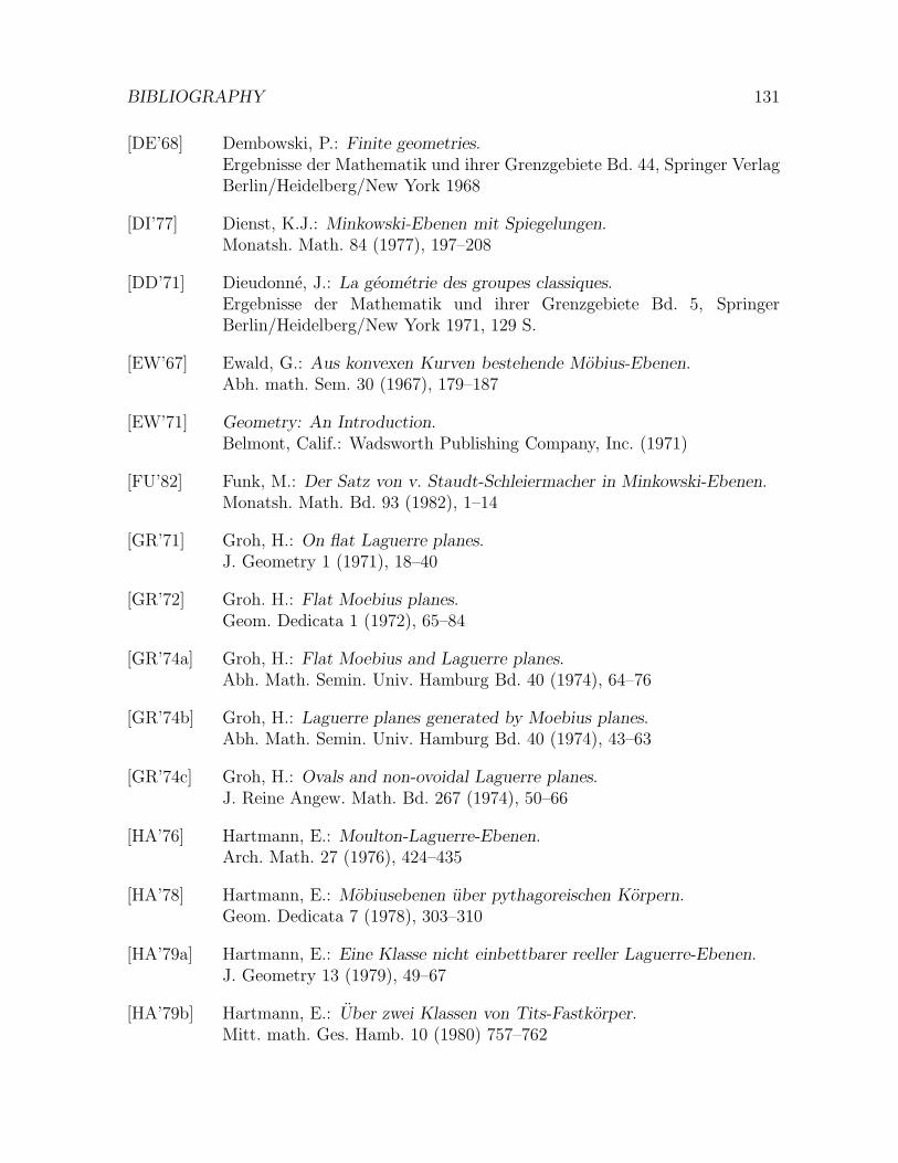
BIBLIOGRAPHY 131
[DE’68] Dembowski, P.: Finite geometries.Ergebnisse der Mathematik und ihrer Grenzgebiete Bd. 44, Springer VerlagBerlin/Heidelberg/New York 1968
[DI’77] Dienst, K.J.: Minkowski-Ebenen mit Spiegelungen.Monatsh. Math. 84 (1977), 197–208
[DD’71] Dieudonne, J.: La geometrie des groupes classiques.Ergebnisse der Mathematik und ihrer Grenzgebiete Bd. 5, SpringerBerlin/Heidelberg/New York 1971, 129 S.
[EW’67] Ewald, G.: Aus konvexen Kurven bestehende Mobius-Ebenen.Abh. math. Sem. 30 (1967), 179–187
[EW’71] Geometry: An Introduction.Belmont, Calif.: Wadsworth Publishing Company, Inc. (1971)
[FU’82] Funk, M.: Der Satz von v. Staudt-Schleiermacher in Minkowski-Ebenen.Monatsh. Math. Bd. 93 (1982), 1–14
[GR’71] Groh, H.: On flat Laguerre planes.J. Geometry 1 (1971), 18–40
[GR’72] Groh. H.: Flat Moebius planes.Geom. Dedicata 1 (1972), 65–84
[GR’74a] Groh, H.: Flat Moebius and Laguerre planes.Abh. Math. Semin. Univ. Hamburg Bd. 40 (1974), 64–76
[GR’74b] Groh, H.: Laguerre planes generated by Moebius planes.Abh. Math. Semin. Univ. Hamburg Bd. 40 (1974), 43–63
[GR’74c] Groh, H.: Ovals and non-ovoidal Laguerre planes.J. Reine Angew. Math. Bd. 267 (1974), 50–66
[HA’76] Hartmann, E.: Moulton-Laguerre-Ebenen.Arch. Math. 27 (1976), 424–435
[HA’78] Hartmann, E.: Mobiusebenen uber pythagoreischen Korpern.Geom. Dedicata 7 (1978), 303–310
[HA’79a] Hartmann, E.: Eine Klasse nicht einbettbarer reeller Laguerre-Ebenen.J. Geometry 13 (1979), 49–67
[HA’79b] Hartmann, E.: Uber zwei Klassen von Tits-Fastkorper.Mitt. math. Ges. Hamb. 10 (1980) 757–762
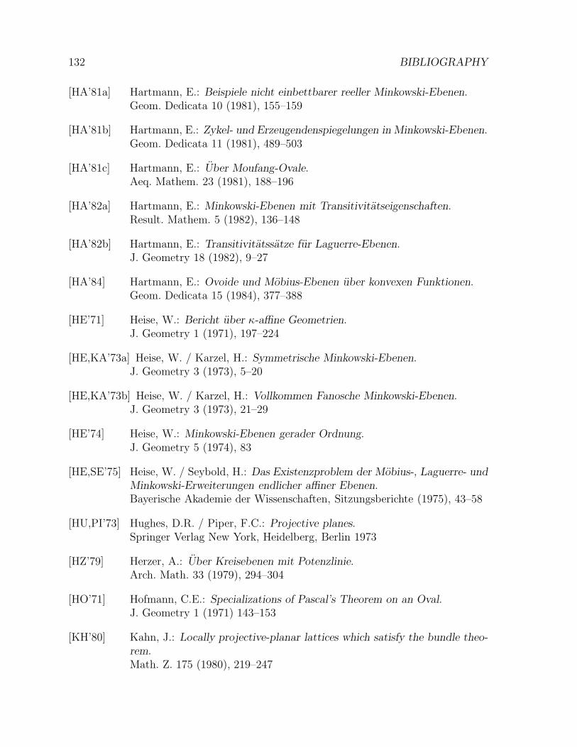
132 BIBLIOGRAPHY
[HA’81a] Hartmann, E.: Beispiele nicht einbettbarer reeller Minkowski-Ebenen.Geom. Dedicata 10 (1981), 155–159
[HA’81b] Hartmann, E.: Zykel- und Erzeugendenspiegelungen in Minkowski-Ebenen.Geom. Dedicata 11 (1981), 489–503
[HA’81c] Hartmann, E.: Uber Moufang-Ovale.Aeq. Mathem. 23 (1981), 188–196
[HA’82a] Hartmann, E.: Minkowski-Ebenen mit Transitivitatseigenschaften.Result. Mathem. 5 (1982), 136–148
[HA’82b] Hartmann, E.: Transitivitatssatze fur Laguerre-Ebenen.J. Geometry 18 (1982), 9–27
[HA’84] Hartmann, E.: Ovoide und Mobius-Ebenen uber konvexen Funktionen.Geom. Dedicata 15 (1984), 377–388
[HE’71] Heise, W.: Bericht uber κ-affine Geometrien.J. Geometry 1 (1971), 197–224
[HE,KA’73a] Heise, W. / Karzel, H.: Symmetrische Minkowski-Ebenen.J. Geometry 3 (1973), 5–20
[HE,KA’73b] Heise, W. / Karzel, H.: Vollkommen Fanosche Minkowski-Ebenen.J. Geometry 3 (1973), 21–29
[HE’74] Heise, W.: Minkowski-Ebenen gerader Ordnung.J. Geometry 5 (1974), 83
[HE,SE’75] Heise, W. / Seybold, H.: Das Existenzproblem der Mobius-, Laguerre- undMinkowski-Erweiterungen endlicher affiner Ebenen.Bayerische Akademie der Wissenschaften, Sitzungsberichte (1975), 43–58
[HU,PI’73] Hughes, D.R. / Piper, F.C.: Projective planes.Springer Verlag New York, Heidelberg, Berlin 1973
[HZ’79] Herzer, A.: Uber Kreisebenen mit Potenzlinie.Arch. Math. 33 (1979), 294–304
[HO’71] Hofmann, C.E.: Specializations of Pascal’s Theorem on an Oval.J. Geometry 1 (1971) 143–153
[KH’80] Kahn, J.: Locally projective-planar lattices which satisfy the bundle theo-rem.Math. Z. 175 (1980), 219–247
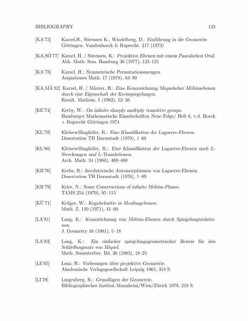
BIBLIOGRAPHY 133
[KA’73] Karzel,H., Sorensen K., Windelberg, D.: Einfuhrung in die Geometrie.Gottingen: Vandenhoeck & Ruprecht. 217 (1973)
[KA,SO’77] Karzel, H. / Sorensen, K.: Projektive Ebenen mit einem Pascalschen Oval.Abh. Math. Sem. Hamburg 36 (1977), 123–125
[KA’78] Karzel, H.: Symmetrische Permutationsmengen.Aequationes Math. 17 (1978), 83–90
[KA,MA’82] Karzel, H. / Maurer, H.: Eine Kennzeichnung Miquelscher Mobiusebenendurch eine Eigenschaft der Kreisspiegelungen.Result. Mathem. 5 (1982), 52–56
[KE’74] Kerby, W.: On infinite sharply multiply transitive groups.Hamburger Mathematische Einzelschriften Neue Folge/ Heft 6, v.d. Hoeck+ Ruprecht Gottingen 1974
[KL’79] Kleinewillinghofer, R.: Eine Klassifikation der Laguerre-Ebenen.Dissertation TH Darmstadt (1979), 1–68
[KL’80] Kleinewillinghofer, R.: Eine Klassifikation der Laguerre-Ebenen nach L-Streckungen und L-Translationen.Arch. Math. 34 (1980), 469–480
[KB’76] Krebs, R.: Involutorische Automorphismen von Laguerre-Ebenen.Dissertation TH Darmstadt (1976), 1–89
[KR’79] Krier, N.: Some Constructions of infinite Mobius-Planes.TAMS 254 (1979), 95–115
[KU’71] Kruger, W.: Kegelschnitte in Moufangebenen.Math. Z. 120 (1971), 41–60
[LA’81] Lang, K.: Kennzeichnung von Mobius-Ebenen durch Spiegelungsrelatio-nen.J. Geometry 16 (1981), 5–18
[LA’83] Lang, K.: Ein einfacher spiegelungsgeometrischer Beweis fur denSchließungssatz von Miquel.Math. Semesterber. Bd. 30 (1983), 18–25
[LE’65] Lenz, H.: Vorlesungen uber projektive Geometrie.Akademische Verlagsgesellschaft Leipzig 1965, 354 S.
[LI’78] Lingenberg, R.: Grundlagen der Geometrie.Bibliographisches Institut Mannheim/Wien/Zurich 1978, 218 S.
134 BIBLIOGRAPHY
[MA’67] Maurer, H.: Mobius- und Laguerre-Geometrien uber schwach konvexenSemiflachen.Math. Zeitschr. 98 (1967), 355–386
[MA’70] Maurer, H.: Spiegelungen an Halbovoiden.Arch. Math. 21 (1970), 411–415
[MA’72] Maurer, H.: Eine Kennzeichnung halbovoidaler Laguerre-Geometrien.J. Reine Angew. Math. 253 (1972), 203–213
[MA’73] Maurer, H.: Zu Punktepaaren symmetrische Ovoide.Arch. Math. 24 (1973), 434–439
[MA’76a] Maurer, H.: Laguerre-Ebenen mit Symmetrien an Punktepaaren undZykeln.J. Geometry 8 (1976), 79–93
[MA’76b] Maurer, H.: Ovoide mit Symmetrien an den Punkten einer Hyperebene.Abh. Math. Sem. Hamburg 45 (1976), 237–244
[MA’77] Maurer, H.: Die Bedeutung des Spiegelungsbegriffs in der Mobius- und derLaguerre-Geometrie.Beitrage zur Geometrischen Algebra (1977), 251–258
[MA’78] Maurer, H.: Involutorische Automorphismen von Laguerre-Ebenen mitgenau zwei Fixpunkten.Monatsh. Math. 86 (1978), 131–142
[MA,ME,NO’80] Maurer, H. / Metz, R. / Nolte, W.: Die Automorphismengruppe derMobius-Geometrie einer Korpererweiterung.Aequationes Math. 21 (1980), 110–112
[MA’81] Maurer, H.: Symmetries of Quadrics.Geometry – von Staudt’s Point of View, Proc. of the NATO AdvancedStudy held at Bad Windsheim 1980, Reidel Publ. Co Dordrecht, Holland1981
[MA’83] Maurer, H.: Permutationsgruppen ohne Pseudoinvolutionen, in derenStandgruppen die Involutionen regular operieren.J. Algebra 82 (1983), 539-545
[PA’71] Payne, E.: A complete determination of translation ovoids in finite desar-guian planes.Accademia Nazionale dei Lincei Serie VIII, Vol. LI, Fasc. 5 (1971), 226–229
BIBLIOGRAPHY 135
[PE’74] Percsy, N.: A characterization of classical Minkowski planes over a perfectfield of characteristics two.J. Geometry 5 (1974), 191–204
[PE’79] Percsy, N.: A Remark on the introduction of coordinates in Minkowskiplanes.J. Geometry 12 (1979), 175–183
[PE’81] Percsy, N.: Finite Minkowski planes in which every circle-symmetry is anautomorphism.Geom. Dedicata 10 (1981), 269–282
[PE’83] Percsy, N.: Les plans de Minkowski possedant des inversions sont Miquel-liens.Simon Stevin 57 (1983), 15–35
[PI’55] Pickert, G.: Projektive Ebenen.Grundl. d. math. Wiss. i. Einzeld. 80, Springer VerlagBerlin/Gottingen/Heidelberg
[QV’52] Qvist, B.: Some remarks concerning curves of the second degree in a finiteplane.Ann. Acad. Sci. Fenn. 134 (1952), 1–27
[RO,VA’73] Roberts, A.W. / Varberg, D.E.: Convex functions.Academic Press 57 New York/London 1973, 287 S.
[SC’80] Schenkel, A.: Topologische Minkowskiebenen.Dissertation, Univ. Erlangen-Nurnberg 1980
[SR’82] Schroder, E.: Ein neuer Winkelbegriff fur die Elementargeometrie.Prax. Math. Heft 9 (1982), 257–267
[SE’55] Segre, B.: Ovals in a finite projective plane.Canad. Journal of Math. 7 (1955), 414–416
[SE’57] Segre, B.: Sui k-archi nei piani finite di caracteristica due.Rev. Math. Pures Appl. 2 (1957), 289–300
[TH’74] Thas, J.A.: On semi ovals and semi ovoids.Geom. Dedicata 3 (1974), 229–231
[TI’62] Tits, J.: Ovoides a translations.Rend. Mat. 21 (1962), 37–59
[WA,SM’35] Waerden, v.d. B.L. / Smid, L.J.: Eine Axiomatik der Kreisgeometrie undder Laguerregeometrie.Math. Ann. 110 (1935), 753–776
136 BIBLIOGRAPHY
[WA’87] Wahling, H.: Theorie der Fastkorper.Thales-Verl. (1987)
[WE’76] Wefelscheid, H.: Zur Charakterisierung einer Klasse von Hyperbelstruk-turen.J. Geometry 9 (1976), 127–133
[WE’77] Wefelscheid, H.: Uber die Automorphismengruppen von Hyperbelstruk-turen.Beitrage zur Geometrischen Algebra (1977), 337–343
[WE’78] Wefelscheid, H.: Verallgemeinerte Minkowski-Geometrie.Contrib. to Geometry Siegen (1978), 397–406
[WE’79] Wefelscheid, H.: Eine Orthogonalitatsbeziehung in Hyperbelstrukturen.Abh. Math. Semin. Univ. Hamb. 48 (1979), 225–230
[WE’81] Wefelscheid, H.: Zur Planaritat von KT-Fastkorpern.Arch. Math. 36 (1981), 302–304
[WI’82a] Wilbrink, H.A.: Finite Minkowski Planes.Geom. Dedicata 12 (1982), 119–129
[WI’82b] Wilbrink, H.A.: Two-transitive Minkowski Planes.Geom. Dedicata 12 (1982), 383–395
[ZA’36a] Zassenhaus, H.: Kennzeichnung endlicher linearer Gruppen als Permuta-tionsgruppen.Abh. Math. Sem. Hamburg 11 (1936), 17–40
[ZA’36b] Zassenhaus, H.: Uber endliche Fastkorper.Abh. Math. Sem. Hamburg 11 (1936), 187–220
[ZE’77] Zeitler, H.: Uber (K,L)-Ebenen.Dissertation, Gesamthochschule Kassel 1977