Embed Size (px)
Citation preview
NOISE DECOMPOSITION FOR STOCHASTIC HODGKIN-HUXLEY MODELS
by
SHUSEN PU
Submitted in partial fulfillment of the requirements
for the degree of Doctor of Philosophy
Dissertation Advisor: Dr. Peter J. Thomas
Department of Mathematics, Applied Mathematics and Statistics
CASE WESTERN RESERVE UNIVERSITY
January, 2021
CASE WESTERN RESERVE UNIVERSITY
SCHOOL OF GRADUATE STUDIES
We hereby approve the thesis of
Shusen Pu
Candidate for the Doctor of Philosophy degree∗.
Prof. Peter J. Thomas
Committee Chair, Advisor
Prof. Daniela Calvetti
Professor of Mathematics
Prof. Erkki Somersalo
Professor of Mathematics
Prof. David Friel
External Faculty, Associate Professor of Neurosciences
Date: October 2, 2020
*We also certify that written approval has been obtained for anyproprietary material contained therein.
i
Table of Contents
Table of Contents . . . . . . . . . . . . . . . . . . . . . . . . . . . . . . . iiList of Tables . . . . . . . . . . . . . . . . . . . . . . . . . . . . . . . . . vList of Figures . . . . . . . . . . . . . . . . . . . . . . . . . . . . . . . . . viAcknowledgement . . . . . . . . . . . . . . . . . . . . . . . . . . . . . . viiiAbstract . . . . . . . . . . . . . . . . . . . . . . . . . . . . . . . . . . . . x
I Introduction and Motivation 1
1 Physiology Background 21.1 Single Cell Neurophysiology . . . . . . . . . . . . . . . . . . . . . . . . . 21.2 Ion Channels . . . . . . . . . . . . . . . . . . . . . . . . . . . . . . . . . 4
2 Foundations of the Hodgkin-Huxley Model 62.1 Membrane Capacitance and Reversal Potentials . . . . . . . . . . . . . . . 72.2 The Membrane Current . . . . . . . . . . . . . . . . . . . . . . . . . . . . 82.3 The Hodgkin-Huxley Model . . . . . . . . . . . . . . . . . . . . . . . . . 9
3 Channel Noise 143.1 Modeling Channel Noise . . . . . . . . . . . . . . . . . . . . . . . . . . . 163.2 Motivation 1: The Need for Efficient Models . . . . . . . . . . . . . . . . 19
4 The Connection Between Variance of ISIs with the Random Gating of IonChannels 224.1 Variability In Action Potentials . . . . . . . . . . . . . . . . . . . . . . . . 224.2 Motivation 2: Understanding the Molecular Origins of Spike Time Variability 23
II Mathematical Framework 31
5 The Deterministic 4-D and 14-D HH Models 325.1 The 4D Hodgkin-Huxley Model . . . . . . . . . . . . . . . . . . . . . . . 355.2 The Deterministic 14D Hodgkin-Huxley Model . . . . . . . . . . . . . . . 36
ii
5.3 Relation Between the 14D and 4D Deterministic HH Models . . . . . . . . 375.4 Local Convergence Rate . . . . . . . . . . . . . . . . . . . . . . . . . . . 47
6 Stochastic 14D Hodgkin-Huxley Models 516.1 Two Stochastic Representations for Stochastic Ion Channel Kinetics . . . . 526.2 Exact Stochastic Simulation of HH Kinetics . . . . . . . . . . . . . . . . . 586.3 Previous Langevin Models . . . . . . . . . . . . . . . . . . . . . . . . . . 616.4 The 14× 28D HH Model . . . . . . . . . . . . . . . . . . . . . . . . . . . 666.5 Stochastic Shielding for the 14D HH Model . . . . . . . . . . . . . . . . . 71
III Model Comparison 78
7 Pathwise Equivalence for a Class of Langevin Models 797.1 When are Two Langevin Equations Equivalent? . . . . . . . . . . . . . . . 807.2 Map Channel-based Langevin Models to Fox and Lu’s Model . . . . . . . . 84
8 Model Comparison 908.1 L1 Norm Difference of ISIs . . . . . . . . . . . . . . . . . . . . . . . . . . 918.2 Two-sample Kolmogorov-Smirnov Test . . . . . . . . . . . . . . . . . . . 96
IV Applications of the 14× 28D Langevin Model 102
9 Definitions, Notations and Terminology 1039.1 The HH Domain . . . . . . . . . . . . . . . . . . . . . . . . . . . . . . . 1039.2 Interspike Intervals and First Passage Times . . . . . . . . . . . . . . . . . 1069.3 Asymptotic phase and infinitesimal phase response curve . . . . . . . . . . 1149.4 Small-noise expansions . . . . . . . . . . . . . . . . . . . . . . . . . . . . 1169.5 Iso-phase Sections . . . . . . . . . . . . . . . . . . . . . . . . . . . . . . 118
10 Noise Decomposition of the 14-D Stochastic HH Model 12210.1 Assumptions for Decomposition of the Full Noise Model . . . . . . . . . . 12410.2 Noise Decomposition Theorem . . . . . . . . . . . . . . . . . . . . . . . . 12710.3 Proof of Theorem 4 . . . . . . . . . . . . . . . . . . . . . . . . . . . . . . 131
11 Decomposition of the Variance of Interspike Intervals 13911.1 Observations on σ2
ISI, and σ2IPI . . . . . . . . . . . . . . . . . . . . . . . . . 142
11.2 Numerical Performance of the Decomposition Theorem . . . . . . . . . . . 147
iii
V Conclusions and Discussion 156
12 Conclusions 15712.1 Summary . . . . . . . . . . . . . . . . . . . . . . . . . . . . . . . . . . . 157
13 Discussions 16013.1 Discrete Gillespie Markov Chain Algorithms . . . . . . . . . . . . . . . . 16013.2 Langevin Models . . . . . . . . . . . . . . . . . . . . . . . . . . . . . . . 16113.3 Model Comparisons . . . . . . . . . . . . . . . . . . . . . . . . . . . . . . 16313.4 Stochastic Shielding Method . . . . . . . . . . . . . . . . . . . . . . . . . 16413.5 Which Model to Use? . . . . . . . . . . . . . . . . . . . . . . . . . . . . . 16513.6 Variance of Interspike Intervals . . . . . . . . . . . . . . . . . . . . . . . . 167
14 Limitations 173
A Table of Common Symbols and Notations 177
B Parameters and Transition Matrices 180
C Diffusion Matrix of the 14D Model 183Bibliography . . . . . . . . . . . . . . . . . . . . . . . . . . . . . . . . . . . . 187
iv

List of Tables
3.1 Number of Na+ and K+ channels . . . . . . . . . . . . . . . . . . . . . . . 15
5.1 Map from 14D to 4D HH model . . . . . . . . . . . . . . . . . . . . . . . 385.2 Map from 4D to 14D HH model . . . . . . . . . . . . . . . . . . . . . . . 39
8.1 Model comparison . . . . . . . . . . . . . . . . . . . . . . . . . . . . . . 94
A.1 Common symbols and notations in this thesis (part I). . . . . . . . . . . . . 177A.2 Common symbols and notations in this thesis (part II). . . . . . . . . . . . 178A.3 Common symbols and notations in this thesis (part III). . . . . . . . . . . . 179
B.1 Parameters used for simulations in this thesis. . . . . . . . . . . . . . . . . 180
v
List of Figures
1.1 Diagrams of neurons . . . . . . . . . . . . . . . . . . . . . . . . . . . . . 31.2 Schematic plot of a typical action potential . . . . . . . . . . . . . . . . . . 5
2.1 HH components . . . . . . . . . . . . . . . . . . . . . . . . . . . . . . . . 102.2 Sample trace of the deterministic HH model . . . . . . . . . . . . . . . . . 13
3.1 Hodgkin-Huxley kinetics . . . . . . . . . . . . . . . . . . . . . . . . . . . 17
4.1 Voltage recordings from intact Purkinje cells . . . . . . . . . . . . . . . . . 244.2 Interdependent variables under current clamp . . . . . . . . . . . . . . . . 26
5.1 4D and 14D HH models . . . . . . . . . . . . . . . . . . . . . . . . . . . 345.2 Convergence to the 4D submanifold . . . . . . . . . . . . . . . . . . . . . 50
6.1 Stochastic shielding under voltage clamp . . . . . . . . . . . . . . . . . . . 726.2 Stochastic shielding under current clamp . . . . . . . . . . . . . . . . . . . 766.3 Robustness of edge-importance ordering under current clamp . . . . . . . . 77
7.1 Pathwise equivalency of 14D HH model and Fox and Lu’s model . . . . . . 89
8.1 Subunit model . . . . . . . . . . . . . . . . . . . . . . . . . . . . . . . . . 958.2 Relative computational efficiency . . . . . . . . . . . . . . . . . . . . . . . 978.3 Logarithm of the ratio of Kolmogorov-Smirnov test statistic . . . . . . . . 100
9.1 Example voltage trace for the 14-D stochastic HH model . . . . . . . . . . 1079.2 Sample trace of the 14× 28D model . . . . . . . . . . . . . . . . . . . . . 1099.3 Example trajectory and the partition of threshold crossing . . . . . . . . . . 1109.4 Sample trace on the limit cycle and its phase function . . . . . . . . . . . . 114
10.1 Approximate decomposition of interspike interval variance . . . . . . . . . 124
11.1 Histogram of voltage recordings and number of spikes as a function ofvoltage threshold . . . . . . . . . . . . . . . . . . . . . . . . . . . . . . . 144
11.2 Standard deviation of the interspike intervals and iso-phase intervals . . . . 146
vi
11.3 Comparison of variance of ISIs (σ2ISI) and IPIs (σ2
IPI) . . . . . . . . . . . . . 14811.4 Numerical performance of the decomposition for the ISI variance for Na+ and
K+ kinetics . . . . . . . . . . . . . . . . . . . . . . . . . . . . . . . . . . 15211.5 Overall performance of the decomposition theorem on ISI variance . . . . . 154
13.1 Variance of ISI using different threshold conditions . . . . . . . . . . . . . 16913.2 Variance of ISI using different thresholds for large noise . . . . . . . . . . 171
vii
Acknowledgement
This thesis represents not only my development in applied mathematics, it is also a
milestone in six years of study at Case Western Reserve University (CWRU). My experi-
ence at CWRU has been a wonderful journey full of amazement. This thesis is the result
of many experiences I have encountered at CWRU from dozens of remarkable individuals
who I sincerely wish to acknowledge.
First and foremost, I would like to thank my advisor, Professor Peter J. Thomas for
his support in both my academic career and personal life. He has been supportive even
before I officially registered at CWRU when we met on the 2014 SIAM conference on
the life sciences. I still remember him sketching the neural spike train and explaining to
me the mathematical models for action potentials, which turned out to be the main focus
of my dissertation. Ever since, Professor Thomas has supported me not only by teaching
me knowledge in computational neuroscience over almost six years, but also academically
and emotionally through the rough road to finish this thesis. Thanks to his great effort in
walking me through every detail of the field and proofreading line by line of all my papers
and thesis. And during the most difficult times when my father left me, he gave me the
moral support and the time that I needed to recover. There are so many things fresh in my
mind and I cannot express how grateful I am for his supervision and support.
I would also like to thank every professor who shared their knowledge and experience
with me, Dr. Daniela Calvetti, Dr. Erkki Somersalo, Dr. Weihong Guo, Dr. Alethea Barbaro,
Dr. Wanda Strychalski, Dr. Wojbor Woyczynski, and Dr. Longhua Zhao.
viii
Especially, I want to thank my committee members Dr. Daniela Calvetti, Dr. Erkki
Somersalo in the Department of Mathematics, Applied Mathematics and Statistics at CWRU,
and Dr. David Friel from the Department of Neurosciences at the Case School of Medicine.
The book on mathematical modeling written by Dr. Daniela Calvetti and Dr. Erkki Som-
ersalo is my first formal encounter with mathematical models for dynamic systems and
stochastic processes. Moreover, I have taken a series of computational oriented courses
offered by Dr. Daniela Calvetti, where she taught me many programming skills and how
to elegantly present my work. I would like to thank Dr. David Friel for his inspiring dis-
cussions during the past few years. All data recordings in this thesis come from Dr. David
Friel’s laboratory, and he taught me a lot of the biophysical background of this dissertation.
Moreover, I want to thank the department and National Science Foundation (grant
DMS-1413770) for their support and sponsorship. The devoted faculty and staff in the
department have been really helpful during my graduate study. I also want to thank my
fellow graduate students for their friendship and support. Especially, Sumanth Nakkireddy,
Alexander Strang, Isaac Oduro, Ben Li, Kai Yin, Alberto Bocchinfuso and Yue Zhang, who
made this journey a lot of fun.
Finally, I would like to dedicate this thesis to my wife Yuanqi Xie and my parents. I
feel extremely fortunate to have such a wonderful family. I could not have accomplished
this without their love and support.
ix
Stochastic Hodgkin-Huxley Models and Noise Decomposition
Abstract
by
SHUSEN PU
In this thesis, we present a natural 14-dimensional Langevin model for the Hodgkin-
Huxley (HH) conductance-based neuron model in which each directed edge in the ion
channel state transition graph acts as an independent noise source, leading to a 14×28 noise
coefficient matrix. We show that (i) the corresponding 14D mean-field ordinary differential
equation system is consistent with the classical 4D representation of the HH system; (ii) the
14D representation leads to a noise coefficient matrix that can be obtained cheaply on each
timestep, without requiring a matrix decomposition; (iii) sample trajectories of the 14D
representation are pathwise equivalent to trajectories of several existing Langevin models,
including one proposed by Fox and Lu in 1994; (iv) our 14D representation give the most
accurate interspike-interval distribution, not only with respect to moments but under both
the L1 and L∞ metric-space norms; and (v) the 14D representation gives an approximation
to exact Markov chain simulations that are as fast and as efficient as all equivalent models.
We combine the stochastic shielding (SS) approximation, introduced by Schmandt and
Galan in 2012, with Langevin versions of the HH model to derive an analytic decom-
position of the variance of the interspike intervals (ISI), based on the mean–return-time
oscillator phase. We prove in theory, and demonstrate numerically, that in the limit of
x
small noise, the variance of the ISI decomposes linearly into a sum of contributions from
each directed edge. Unlike prior analyses, our results apply to current clamp rather than
voltage clamp conditions. Under current clamp, a stochastic conductance-based model is
an example of a piecewise-deterministic Markov process. Our theory is exact in the limit of
small channel noise. Through numerical simulations we demonstrate its applicability over a
range from small to moderate noise levels. We show numerically that the SS approximation
has a high degree of accuracy even for larger, physiologically relevant noise levels.
xi

Part I
Introduction and Motivation
1
Chapter 1
Physiology Background
There is no scientific study more vital to man than the study of his own brain.
Our entire view of the universe depends on it.
– Francis Crick
1.1 Single Cell Neurophysiology
The human brain is the command center for the human nervous system, which controls
most of the activities of the body, receiving and analyzing information from the body’s
sensory organs, and sending out decision information to the rest of the body. The human
brain contains billions of nerve cells interconnected by trillions of synapses, that commu-
nicate with one another and with peripheral systems (sensory organs, muscles) through
transient spikes in transmembrane voltages called “action potentials”. Fig. 1.1 shows three
types of neurons. In a neuron, the dendrite receives inputs from other neurons, and the axon
carries the neuronal output to other cells [22].
2
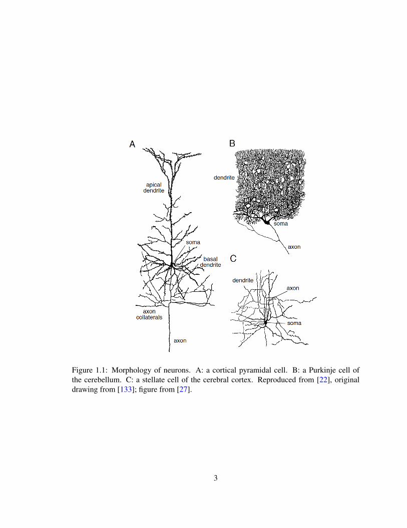
Figure 1.1: Morphology of neurons. A: a cortical pyramidal cell. B: a Purkinje cell ofthe cerebellum. C: a stellate cell of the cerebral cortex. Reproduced from [22], originaldrawing from [133]; figure from [27].
3
1.2 Ion Channels
There are a wide variety of pore-forming membrane proteins, namely ion channels, that
allow ions, such as sodium (Na+), potassium (K+), calcium (Ca2+), and chloride (Cl−),
to pass through the cell. Ion channels control the flow of ions across the cell membrane
by opening and closing in response to voltage changes and to both internal and external
signals. Neurons maintain a voltage difference between the exterior and interior of the cell,
which is called the membrane potential. Under resting conditions, a typical voltage across
an neuron cell membrane is about −70 mV. Pumps spanning the cell membrane maintain
a concentration difference that support this membrane potential. More specifically, under
the resting state, the concentration of Na+ is much higher outside a neuron than inside,
while the concentration of K+ is significantly higher inside the neuron than its extracellular
environment [22].
An action potential occurs when the membrane potential at a specific location of the
cell rapidly changes. Action potentials are generated by voltage-gated ion channels in
the cell’s membrane. These ion channels are shut when the membrane potential is near
the resting potential and they rapidly open when the membrane potential increases to a
threshold voltage, which leads a depolarization of the membrane potential [8]. During the
depolarization, the sodium channels open, which produces a further rise in the membrane
potential. The influx of sodium ions causes the polarity of the membrane to reverse, which
rapidly leads to the inactivation of sodium channels and activation of potassium channels.
There is a transient negative shift after an action potential has occurred, which is called
the after hyperpolarization (AHP). Action potentials (or “spikes”) are generally thought to
carry information via their timing (as opposed to their magnitude or duration). Figure 1.2
gives an schematic plot of a typical action potential.
4
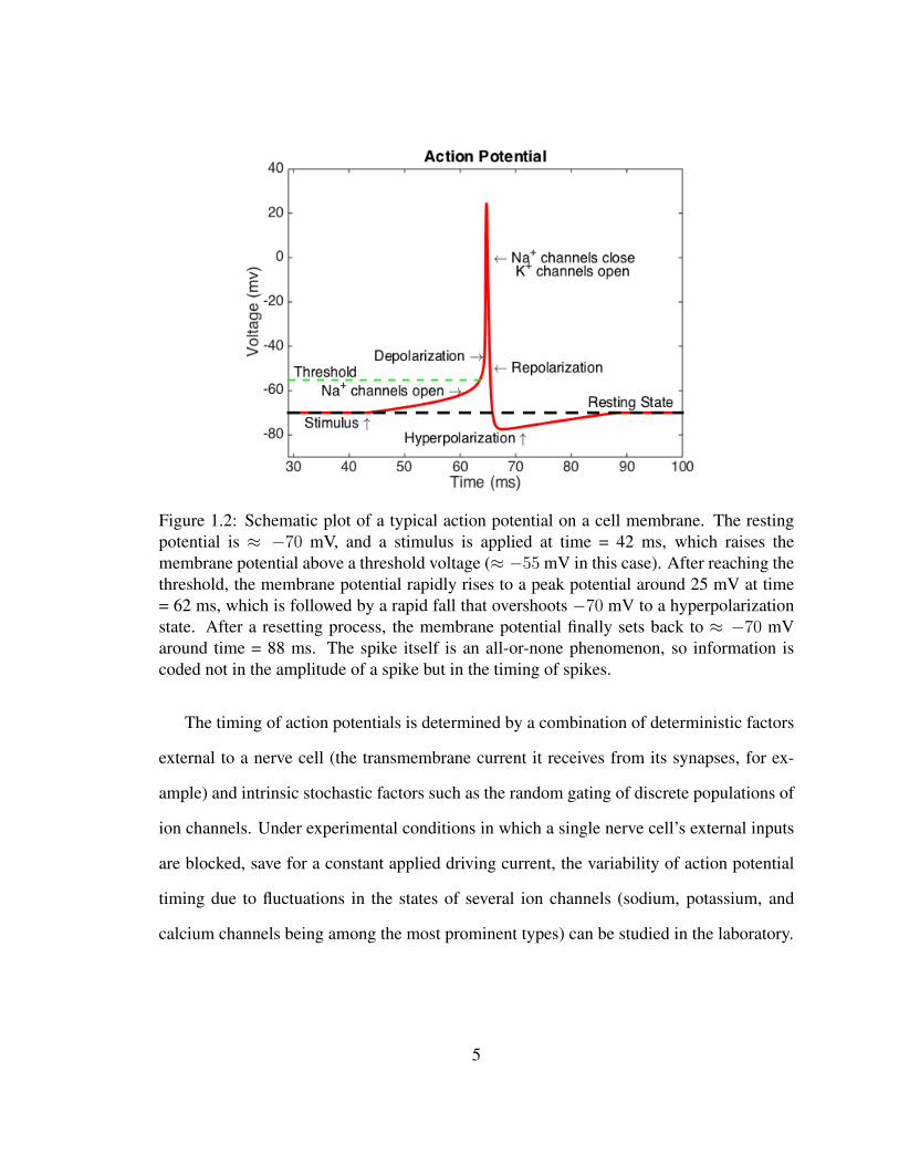
Figure 1.2: Schematic plot of a typical action potential on a cell membrane. The restingpotential is ≈ −70 mV, and a stimulus is applied at time = 42 ms, which raises themembrane potential above a threshold voltage (≈ −55 mV in this case). After reaching thethreshold, the membrane potential rapidly rises to a peak potential around 25 mV at time= 62 ms, which is followed by a rapid fall that overshoots −70 mV to a hyperpolarizationstate. After a resetting process, the membrane potential finally sets back to ≈ −70 mVaround time = 88 ms. The spike itself is an all-or-none phenomenon, so information iscoded not in the amplitude of a spike but in the timing of spikes.
The timing of action potentials is determined by a combination of deterministic factors
external to a nerve cell (the transmembrane current it receives from its synapses, for ex-
ample) and intrinsic stochastic factors such as the random gating of discrete populations of
ion channels. Under experimental conditions in which a single nerve cell’s external inputs
are blocked, save for a constant applied driving current, the variability of action potential
timing due to fluctuations in the states of several ion channels (sodium, potassium, and
calcium channels being among the most prominent types) can be studied in the laboratory.
5
Chapter 2
Foundations of the Hodgkin-Huxley
Model
The Nobel Prize in Physiology or Medicine 1963 is awarded jointly to Sir John
Carew Eccles, Alan Lloyd Hodgkin and Andrew Fielding Huxley “for their dis-
coveries concerning the ionic mechanisms involved in excitation and inhibition
in the peripheral and central portions of the nerve cell membrane.”
– Nobel Prize Committee, 1963
By using voltage clamp experiments and varying extracellular sodium and potassium
concentrations, Alan Hodgkin and Andrew Huxley described a model in 1952 to explain
the ionic mechanisms underlying the initiation and propagation of action potentials. The
Hodgkin-Huxley (HH) model is a set of four nonlinear ordinary differential equations
that approximates the electrical characteristics of neurons firing. They received the 1963
Nobel Prize in Physiology or Medicine for their ground-breaking work on modeling neuron
spikes. In this section, we will first review essential components of the HH model, includ-
6
ing the membrane capacitance, reversal potentials, active conductances, and membrane
current. Then, we will present the mathematical framework of the HH model.
2.1 Membrane Capacitance and Reversal Potentials
Ionic pumps embedded in the membranes of nerve cells typically maintain a negative
charge on the inside surface of the cell membrane, and a balancing positive charge on its
outside surface. This charge imbalance creates a voltage difference V between the inside
and outside of the cell. Specifically, the lipid bilayer of the cell membrane forms a thin
insulator that separates two electrolytic media, the extracellular space and the cytoplasm
[51]. The specific membrane capacitance Cm, the potential across the membrane V , and
the amount of the excess charge density Q (per area) are related by the equation Q = CmV
[1]. Given that the thickness of the membrane is a constant, the total membrane capacitance
cm of a cell is a quantity directly proportional to the membrane surface area and the
properties of the membrane. Therefore, the total membrane capacitance is cm = CmA,
where Cm is the per area membrane capacitance (typically in units of µF/cm2) and A is
the area (typically in units of cm2). The capacitance per unit area of membrane, Cm, is
approximately the same for all neurons with Cm ≈ 10nF/mm2.
The membrane capacitance can be used to determine the current required to change the
membrane potential at a given rate. More specifically, the relation between the change in
voltage and charge can be written as
CmdV
dt=dQ
dt. (2.1)
Equation 2.1 plays an important role in the formulation of the HH model.
7
The reversal potential for a channel is the voltage at which the net current through the
channel is zero. The reversal potential is determined by the difference of concentration of
ions inside the cell, [C]in, and the concentration outside the cell, [C]out. The Nernst equation
[22] for the reversal potential can be written as
V =RT
zFlog
[C]in[C]out
, (2.2)
where R is the universal gas constant: R = 8.31 JK−1mol−1, T is the temperature in
Kelvins, F is the Faraday constant, and z is the charge of the ion species (z = +1 for
Na+ and K+, −1 for Cl−, and z = +2 for Ca2+). The reversal potential for a K+channel,
VK, typically falls in the range between -70 and -90 mV. The reversal potential for Na+, VNa,
is 50 mV or higher. Throughout this thesis, we will use VK = −77mV and VNa = 50mV
for all numerical simulations.
2.2 The Membrane Current
The membrane current of a neuron is the total current flowing across the membrane through
all ion channels [22]. The total membrane current is determined by including all currents
resulting from different types of channels within the cell membrane. To make it comparable
for neurons with different sizes, the membrane current per unit area of cell membrane
is conveniently used, which we define as Im. The total membrane current is obtained
from the current per unit area Im by multiplying by the total surface area of the cell. For
each ion channel, the current depends approximately linearly on the difference between the
membrane potential and its reversal potential, Vion.1 Given the conductance per unit area,
1Here we followed the standard convention that equates “ion channels” with “ion”; in particular, we donot consider nonspecific ion channels.
8
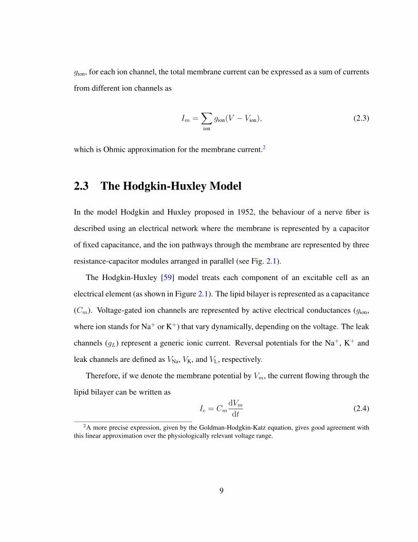
gion, for each ion channel, the total membrane current can be expressed as a sum of currents
from different ion channels as
Im =∑ion
gion(V − Vion), (2.3)
which is Ohmic approximation for the membrane current.2
2.3 The Hodgkin-Huxley Model
In the model Hodgkin and Huxley proposed in 1952, the behaviour of a nerve fiber is
described using an electrical network where the membrane is represented by a capacitor
of fixed capacitance, and the ion pathways through the membrane are represented by three
resistance-capacitor modules arranged in parallel (see Fig. 2.1).
The Hodgkin-Huxley [59] model treats each component of an excitable cell as an
electrical element (as shown in Figure 2.1). The lipid bilayer is represented as a capacitance
(Cm). Voltage-gated ion channels are represented by active electrical conductances (gion,
where ion stands for Na+ or K+) that vary dynamically, depending on the voltage. The leak
channels (gL) represent a generic ionic current. Reversal potentials for the Na+, K+ and
leak channels are defined as VNa, VK, and VL, respectively.
Therefore, if we denote the membrane potential by Vm, the current flowing through the
lipid bilayer can be written as
Ic = CmdVmdt
(2.4)
2A more precise expression, given by the Goldman-Hodgkin-Katz equation, gives good agreement withthis linear approximation over the physiologically relevant voltage range.
9
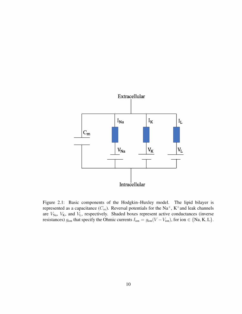
Figure 2.1: Basic components of the Hodgkin–Huxley model. The lipid bilayer isrepresented as a capacitance (Cm). Reversal potentials for the Na+, K+and leak channelsare VNa, VK, and VL, respectively. Shaded boxes represent active conductances (inverseresistances) gion that specify the Ohmic currents Iion = gion(V −Vion), for ion ∈ Na,K,L.
10
and the current through a given ion channel is a product
Iion = gion(Vm − Vion). (2.5)
The original HH model only considered the Na+ and K+ currents and a leak current,
therefore, the total current through the membrane is
I = CmdVmdt
+ gK(Vm − VK) + gNa(Vm − VNa) + gL(Vm − VL) (2.6)
where I is the total membrane current per unit area, Cm is the membrane capacitance per
unit area, gK and gNa are the potassium and sodium conductances per unit area. VK and VNa
are the potassium and sodium reversal potentials, and gL and VL are the leak conductance
per unit area and leak reversal potential, respectively. Appendix B has a complete list of
parameters.
Using a series of voltage clamp experiments, and by numerically fitting parameters,
Hodgkin and Huxley [59] developed a set of four ordinary differential equations as
Cdv
dt= −gNam
3h(v − VNa)− gKn4(v − VK)− gL(v − VL) + Iapp, (2.7)
dm
dt= αm(v)(1−m)− βm(v)m, (2.8)
dh
dt= αh(v)(1− h)− βh(v)h, (2.9)
dn
dt= αn(v)(1− n)− βn(v)n, (2.10)
where v is the membrane potential, Iapp is the applied current, and 0 ≤ m,n, h ≤ 1 are di-
mensionless gating variables associated with the Na+ and K+ channels. The constant gion is
the maximal value of the conductance for the sodium and potassium channel, respectively.
11
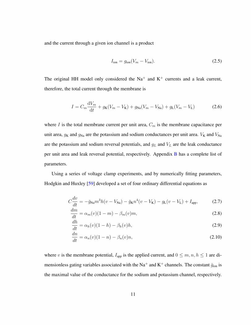
Parameters Vion and C are the ionic reversal potentials and capacitance, respectively. The
quantities αx and βx, x ∈ m,n, h are the voltage-dependent per capita transition rates,
defined as
αm(v) =0.1(25− v)
exp(2.5− 0.1v)− 1, (2.11)
βm(v) = 4 exp(−v/18), (2.12)
αh(v) = 0.07 exp(−v/20), (2.13)
βh(v) =1
exp(3− 0.1v) + 1, (2.14)
αn(v) =0.01(10− v)
exp(1− 0.1v)− 1, (2.15)
βn(v) = 0.125 exp(−v/80). (2.16)
Fig. 2.2 shows the voltage component of a regular spiking trajectory of the HH equa-
tions with constant driving current injection of I = 10 nA/cm2.
12
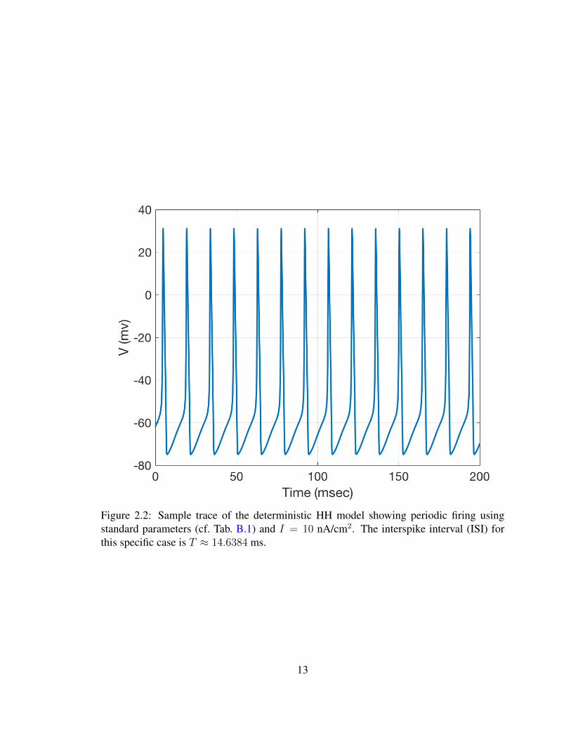
Figure 2.2: Sample trace of the deterministic HH model showing periodic firing usingstandard parameters (cf. Tab. B.1) and I = 10 nA/cm2. The interspike interval (ISI) forthis specific case is T ≈ 14.6384 ms.
13
Chapter 3
Channel Noise
The probabilistic gating of voltage-dependent ion channels is a source of electri-
cal “channel noise” in neurons. This noise has long been implicated in limiting
the reliability of neuronal responses to repeated presentations of identical stimuli.
– White, Rubinstein and Kay [126]
Nerve cells communicate with one another, process sensory information, and control
motor systems through transient voltage pulses, or spikes. At the single-cell level, neurons
exhibit a combination of deterministic and stochastic behaviors. In the supra-threshold
regime, the regular firing of action potentials under steady current drive suggests limit
cycle dynamics, with the precise timing of voltage spikes perturbed by noise. Variability
of action potential timing persists even under blockade of synaptic connections, consistent
with an intrinsically noisy neural dynamics arising from the random gating of ion channel
populations, or “channel noise” [126].
Channel noise arises from the random opening and closing of finite populations of ion
channels embedded in the cell membranes of individual nerve cells, or localized regions of
14
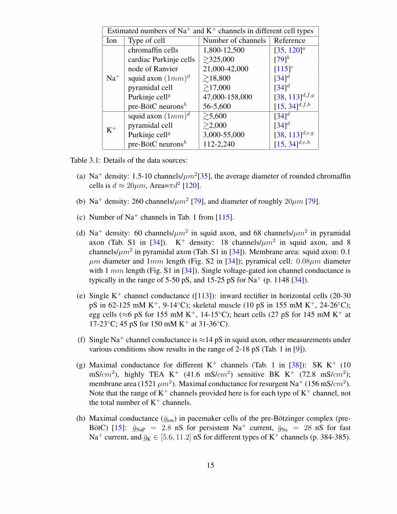
Estimated numbers of Na+ and K+ channels in different cell typesIon Type of cell Number of channels Reference
Na+
chromaffin cells 1,800-12,500 [35, 120]a
cardiac Purkinje cells &325,000 [79]b
node of Ranvier 21,000-42,000 [115]c
squid axon (1mm)d &18,800 [34]d
pyramidal cell &17,000 [34]d
Purkinje cellg 47,000-158,000 [38, 113]d,f,g
pre-BotC neuronsh 56-5,600 [15, 34]d,f,h
K+
squid axon (1mm)d &5,600 [34]d
pyramidal cell &2,000 [34]d
Purkinje cellg 3,000-55,000 [38, 113]d,e,g
pre-BotC neuronsh 112-2,240 [15, 34]d,e,h
Table 3.1: Details of the data sources:
(a) Na+ density: 1.5-10 channels/µm2[35], the average diameter of rounded chromaffincells is d ≈ 20µm, Area=πd2 [120].
(b) Na+ density: 260 channels/µm2 [79], and diameter of roughly 20µm [79].
(c) Number of Na+ channels in Tab. 1 from [115].
(d) Na+ density: 60 channels/µm2 in squid axon, and 68 channels/µm2 in pyramidalaxon (Tab. S1 in [34]). K+ density: 18 channels/µm2 in squid axon, and 8channels/µm2 in pyramidal axon (Tab. S1 in [34]). Membrane area: squid axon: 0.1µm diameter and 1mm length (Fig. S2 in [34]); pyramical cell: 0.08µm diameterwith 1 mm length (Fig. S1 in [34]). Single voltage-gated ion channel conductance istypically in the range of 5-50 pS, and 15-25 pS for Na+ (p. 1148 [34]).
(e) Single K+ channel conductance ([113]): inward rectifier in horizontal cells (20-30pS in 62-125 mM K+, 9-14C); skeletal muscle (10 pS in 155 mM K+, 24-26C);egg cells (≈6 pS for 155 mM K+, 14-15C); heart cells (27 pS for 145 mM K+ at17-23C; 45 pS for 150 mM K+ at 31-36C).
(f) Single Na+ channel conductance is≈14 pS in squid axon, other measurements undervarious conditions show results in the range of 2-18 pS (Tab. 1 in [9]).
(g) Maximal conductance for different K+ channels (Tab. 1 in [38]): SK K+ (10mS/cm2), highly TEA K+ (41.6 mS/cm2) sensitive BK K+ (72.8 mS/cm2);membrane area (1521 µm2). Maximal conductance for resurgent Na+ (156 mS/cm2).Note that the range of K+ channels provided here is for each type of K+ channel, notthe total number of K+ channels.
(h) Maximal conductance (gion) in pacemaker cells of the pre-Botzinger complex (pre-BotC) [15]: gNaP = 2.8 nS for persistent Na+ current, gNa = 28 nS for fastNa+ current, and gK ∈ [5.6, 11.2] nS for different types of K+ channels (p. 384-385).
15
axons or dendrites. Electrophysiological and neuroanatomical measurements do not typi-
cally provide direct measures of the sizes of ion channel populations. Rather, the size of ion
channel populations must be inferred indirectly from other measurements. Several papers
report the density of sodium or potassium channels per area of cell membrane [34, 35, 79].
Multiplying such a density by an estimate of the total membrane area of a cell gives one
estimate for the size of a population of ion channels. Sigworth [115] pioneered statistical
measures of ion channel populations based on the mean and variance of current fluctuations
observed in excitable membranes, for instance in the isolated node of Ranvier in axons of
the frog. Single-channel recordings [85] allowed direct measurement of the “unitary”,
or single–channel-conductance, goNa or goK. Most conductance-based, ordinary differential
equations models of neural dynamics incorporate maximal conductance parameters (gNa or
gK) which nominally represents the conductance that would be present if all channels of a
given type were open. The ratio of g to go thus gives an indirect estimate of the number
of ion channels in a specific cell type. Tab. 3.1 summarizes a range of estimates for ion
channel populations from several sources in the literature. Individual cells range from 50
to 325,000 channels for each type of ion. In §11.2 of this thesis, we will consider effective
channel populations spanning this entire range (cf. Figs 11.3, 11.4).
3.1 Modeling Channel Noise
Hodgkin and Huxley’s quantitative model for active sodium and potassium currents produc-
ing action potential generation in the giant axon of Loligo [59] suggested an underlying sys-
tem of gating variables consistent with a multi-state Markov process description [58]. The
discrete nature of individual ion channel conductances was subsequently experimentally
confirmed [85]. Following this work, numerical studies of high-dimensional discrete-state,
16
14αn
2βnN1
n03
3αn42βnN2
n15
2αn63βnN3
n27
αn
84βnN4
n3
N5
n4
K+ Channel
m003
3αm4βmM1
Na+ Channel
m107
2αm8
2βmM2
Na+ Channel
m2011
αm
123βmM3
Na+ Channel
M4
m30
m0115
3αm16βm
M5
m1117
2αm18
2βm
M6
m2119
αm
203βm
M7 M8
m31
1
αh
2
βh
5
αh
6
βh
9
αh
10
βh
13
αh
14
βh
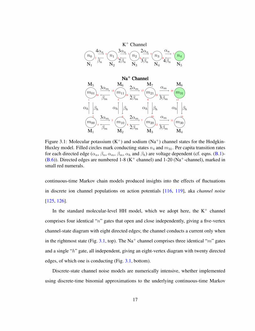
Figure 3.1: Molecular potassium (K+) and sodium (Na+) channel states for the Hodgkin-Huxley model. Filled circles mark conducting states n4 and m31. Per capita transition ratesfor each directed edge (αn, βn, αm, βm, αh and βh) are voltage dependent (cf. eqns. (B.1)-(B.6)). Directed edges are numbered 1-8 (K+ channel) and 1-20 (Na+-channel), marked insmall red numerals.
continuous-time Markov chain models produced insights into the effects of fluctuations
in discrete ion channel populations on action potentials [116, 119], aka channel noise
[125, 126].
In the standard molecular-level HH model, which we adopt here, the K+ channel
comprises four identical “n” gates that open and close independently, giving a five-vertex
channel-state diagram with eight directed edges; the channel conducts a current only when
in the rightmost state (Fig. 3.1, top). The Na+ channel comprises three identical “m” gates
and a single “h” gate, all independent, giving an eight-vertex diagram with twenty directed
edges, of which one is conducting (Fig. 3.1, bottom).
Discrete-state channel noise models are numerically intensive, whether implemented
using discrete-time binomial approximations to the underlying continuous-time Markov
17
process [102, 116] or continuous-time hybrid Markov models with exponentially distributed
state transitions and continuously varying membrane potential. The latter were intro-
duced by [18] and are in principle exact [4]. Under voltage-clamp conditions the hybrid
conductance-based model reduces to a time-homogeneous Markov chain [19] that can
be simulated using standard methods such as Gillespie’s exact algorithm [46, 47]. Even
with this simplification, such Markov Chain (MC) algorithms are numerically expensive
to simulate with realistic population sizes of thousands of channels or greater. Therefore,
there is an ongoing need for efficient and accurate approximation methods.
Following Clay and DeFelice’s exposition of continuous time Markov chain implemen-
tations, [39] introduced a Fokker-Planck equation (FPE) framework that captured the first
and second order statistics of HH ion channel dynamics in a 14-dimensional representation.
Taking into account conservation of probability, one needs four variables to represent
the population of K+ channels, seven for Na+, and one for voltage, leading to a 12-
dimensional state space description. The resulting high-dimensional partial differential
equation is impractical to solve numerically. However, as Fox and Lu observed, “to every
Fokker-Planck description, there is associated a Langevin description” [39]. They therefore
introduced a Langevin stochastic differential equation of the form:
CdV
dt= Iapp(t)− gNaM8 (V − VNa)− gKN5 (V − VK)− gleak(V − Vleak), (3.1)
dM
dt= ANaM + S1ξ1, (3.2)
dN
dt= AKN + S2ξ2, (3.3)
where C is the capacitance, Iapp is the applied current, maximal conductances are denoted
gion, with Vion being the associated reversal potential, and ohmic leak current gleak(V −Vleak).
M ∈ R8 and N ∈ R5 are vectors for the fractions of Na+ and K+ channels in each
18
state, with M8 representing the open channel fraction for Na+, and N5 the open channel
fraction for K+ (Fig. 3.1). Vectors ξ1(t) ∈ R8 and ξ2(t) ∈ R5 are independent Gaussian
white noise processes with zero mean and unit variances 〈ξ1(t)ξᵀ1(t′)〉 = I8 δ(t − t′) and
〈ξ2(t)ξᵀ2(t′)〉 = I5 δ(t − t′). The state-dependent rate matrices ANa and AK are given in
eqns. (5.10) and (5.11). In Fox and Lu’s formulation, S must satisfy S =√D, where D
is a symmetric, positive semi-definite k × k “diffusion matrix” (see Appendix C for the D
matrices for the standard HH K+ and Na+ channels). We will refer to the 14-dimensional
Langevin equations (3.1)-(3.3), with S =√D, as the “Fox-Lu” model.
3.2 Motivation 1: The Need for Efficient Models
The original Fox-Lu model, later called the “conductance noise model” by [49], did not
see widespread use until gains in computing speed made the square root calculations more
feasible. Seeking a more efficient approximation, [39] also introduced a four-dimensional
Langevin version of the HH model. This model was systematically studied in [40] which
can be written as follows:
CdV
dt= Iapp(t)− gNam
3h (V − VNa)− gKn4 (V − VK)
−gleak(V − Vleak) (3.4)
dx
dt= αx(1− x)− βxx+ ξx(t), where x = m,h, or, n. (3.5)
where ξx(t) are Gaussian processes with covariance function
E[ξx(t), ξx(t′)] =
αx(1− x) + βxx
Nδ(t− t′). (3.6)
19
Here N represents the total number of Na+channels (respectively, the total number of
K+channels) and δ(·) is the Dirac delta function. This model, referred as the “subunit noise
model” by [49], has been widely used as an approximation to MC ion channel models
(see references in [12, 49]). For example, [103] used this approximation to investigate
stochastic resonance and coherence resonance in forced and unforced versions of the HH
model (e.g. in the excitable regime). However, the numerical accuracy of this method was
criticized by several studies [12, 81], which found that its accuracy does not improve even
with increasing numbers of channels.
Although more accurate approximations based on Gillespie’s algorithm (using a piece-
wise constant propensity approximation, [12, 81]) and even based on exact simulations
[4, 18, 87] became available, they remained prohibitively expensive for large network
simulations. Meanwhile, Goldwyn and Shea-Brown’s rediscovery of Fox and Lu’s earlier
conductance based model [48, 49] launched a flurry of activity seeking the best Langevin-
type approximation. The paper [49] introduced a faster decomposition algorithm to sim-
ulate equations (3.1)-(3.3), and showed that Fox and Lu’s method accurately captured
the fractions of open channels and the inter-spike interval (ISI) statistics, in comparison
with Gillespie-type Monte Carlo (MC) simulations. However, despite the development of
efficient singular value decomposition based algorithms for solving S =√D, this step still
causes a bottleneck in the algorithms based on [39, 48, 49].
The persistent need for fast and accurate simulation methods is the first main motivation
of this thesis work. Many variations on Fox and Lu’s 1994 Langevin model have been pro-
posed in recent years [20, 21, 41, 56, 60, 61, 73, 90, 93] including Goldwyn et al’s work [48,
49], each with its own strengths and weaknesses. One class of methods imposes projected
boundary conditions [20, 21]; as we will show in §8, this approach leads to an inaccurate
interspike interval distribution, and is inconsistent with a natural multinomial invariant
20

manifold structure for the ion channels. Several methods implement correlated noise at
the subunit level, as in (3.5)-(3.6) [40, 55, 56, 73]. In the subunit model (cf. eqn. (3.5)) a
single noise source represents the fluctuations associated with the gating variable x (x ∈
m,n, h). However, if one recognizes that, at the molecular level, the individual directed
edges in Fig. 3.1 represent the independent noise sources in ion channel dynamics, then it
becomes clear that the subunit noise model obscures the biophysical origin of ion channel
fluctuations. Some methods introduce the noisy dynamics at the level of edges rather
than nodes, but lump reciprocal edges together into pairs [21, 60, 90, 93]. This approach
implicitly assumes, in effect, that the ion channel probability distribution satisfies a detailed
balance (or microscropic reversibility) condition. However, while detailed balance holds
for the HH model under stationary voltage clamp, this condition is violated during active
spiking. Finally, the stochastic shielding approximation [102, 104, 105] does not have a
natural formulation in the representation associated with an n× n noise coefficient matrix
S; in the cases of rectangular S matrices used in [21, 90] stochastic shielding can only be
applied to reciprocal pairs of edges. We will elaborate on these points in §12.
21
Chapter 4
The Connection Between Variance of
ISIs with the Random Gating of Ion
Channels
4.1 Variability In Action Potentials
At the single-cell level, neurons exhibit a combination of deterministic and stochastic
behaviors. In the supra-threshold regime, the action potentials under steady current drive
suggests limit cycle dynamics, with the precise timing of voltage spikes perturbed by noise.
Variability of action potential timing persists even under blockade of synaptic connections,
consistent with an intrinsically noisy neural dynamics arising from the random gating of ion
channel populations, or “channel noise” [126]. Channel noise can have a significant effect
on spike generation [78, 107], propagation along axons [33], and spontaneous (ectopic)
action potential generation in the absence of stimulation [88]. At the network level, channel
22
noise can drive endogenous variability of vital rhythms such as respiratory activity [134].
Understanding the molecular origins of spike time variability may shed light on several
phenomena in which channel noise plays a role. For example, microscopic noise can give
rise to a stochastic resonance behavior [103], and can contribute to cellular- and systems-
level timing changes in the integrative properties of neurons [26]. Jitter in spike times under
steady drive may be observed in neurons from the auditory system [45, 50, 83] as well as
in the cerebral cortex [78] and may play a role in both fidelity of sensory information
processing and in precision of motor control [107].
4.2 Motivation 2: Understanding the Molecular Origins
of Spike Time Variability
As a motivating example for this dissertation, channel noise is thought to underlie jitter
in spike timing observed in cerebellar Purkinje cells recorded in vitro from the “leaner
mouse”, a P/Q-type calcium channel mutant with profound ataxia [123]. Purkinje cells fire
Na+ action potentials spontaneously [76, 77], and may do so at a very regular rate [123],
even in the absence of synaptic input (cf. Fig. 4.1 A and C). Mutations in an homologous
human calcium channel gene are associated with episodic ataxia type II, a debilitating form
of dyskinesia [94, 97]. Previous work has shown that the leaner mutation increases the
variability of spontaneous action potential firing in Purkinje cells [91, 123] (Fig. 4.1 B and
D). It has been proposed that increased channel noise akin to that observed in the leaner
mutant plays a mechanistic role in this human disease [123].
To understand the underlying mechanisms for the different firing properties in wild type
and the leaner mutant, a model with biological fidelity is desired. For example, in addition
to fast channel noise due to sodium and potassium channels, fluctuations of electrical
23
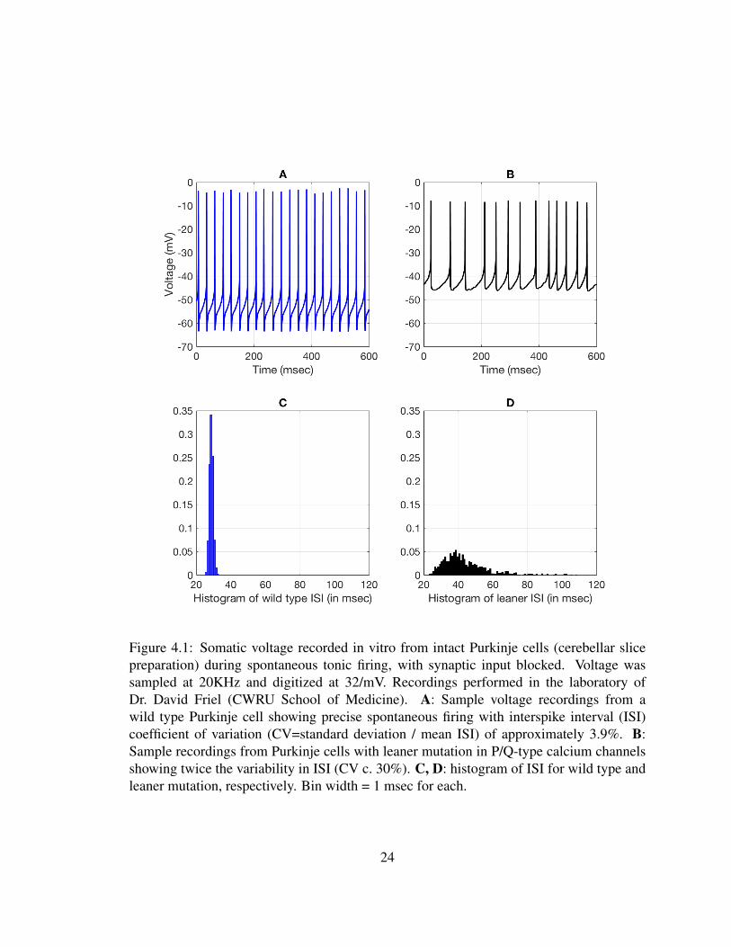
Figure 4.1: Somatic voltage recorded in vitro from intact Purkinje cells (cerebellar slicepreparation) during spontaneous tonic firing, with synaptic input blocked. Voltage wassampled at 20KHz and digitized at 32/mV. Recordings performed in the laboratory ofDr. David Friel (CWRU School of Medicine). A: Sample voltage recordings from awild type Purkinje cell showing precise spontaneous firing with interspike interval (ISI)coefficient of variation (CV=standard deviation / mean ISI) of approximately 3.9%. B:Sample recordings from Purkinje cells with leaner mutation in P/Q-type calcium channelsshowing twice the variability in ISI (CV c. 30%). C, D: histogram of ISI for wild type andleaner mutation, respectively. Bin width = 1 msec for each.
24
activity in PCs may be subject to the effects of slow noise processes such as stochasticity
of calcium channels, calcium-gated potassium channels, and dendritic filtering. Cerebellar
Purkinje cells have been studied using models with a wide range of complexity, from
models with thousands of subcellular compartments each with multiple gating variables and
voltage [23, 24, 25] to “reduced” models with only dozens of compartments [38] as well as
models with as few as five dynamical variables [36]. The currents at work in Purkinje cells
have also been subject to detailed modeling, including “resurgent” sodium current [17, 98],
multiple types of potassium currents [37, 66], calcium currents [37, 82] and calcium-
dependent potassium currents [37]. In order to pave the way for tackling more complex
models, in this thesis we restrict attention to a simpler, single-compartment conductance-
based model, the canonical excitable membrane model originating with Hodgkin and Hux-
ley [59].
Despite its practical importance, a quantitative understanding of distinct molecular
sources of macroscopic timing variability remains elusive, even for the HH model. As
the second main motivation of this thesis, we would like to study the quantitative con-
nection between the molecular-level ion channel transitions to the macroscopic variability
of timing in membrane action potentials. Significant theoretical attention has been paid
to the variance of phase response curves and interspike interval (ISI) variability. Most
analytical studies are based on the integrate-and-fire model [13, 74, 122], except [31],
which perturbs the voltage of a conductance-based model with a white noise current rather
than through biophysically-based channel noise. Standard models of stochastic ion channel
kinetics comprise hybrid stochastic systems. As illustrated in Fig. 4.2, the membrane
potential evolves deterministically, given the transmembrane currents; the currents are
determined by the ion channel state; the ion channel states fluctuate stochastically with
opening and closing rates that depend on the voltage [4, 10, 14, 92]. This closed-loop
25
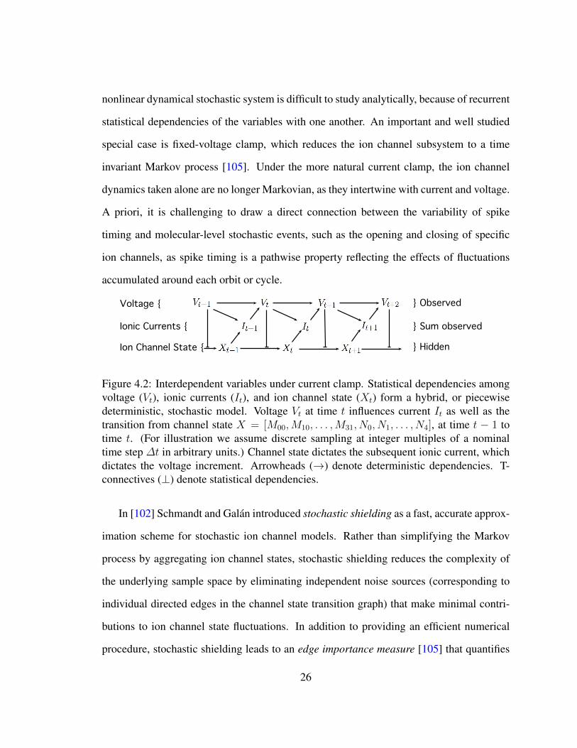
nonlinear dynamical stochastic system is difficult to study analytically, because of recurrent
statistical dependencies of the variables with one another. An important and well studied
special case is fixed-voltage clamp, which reduces the ion channel subsystem to a time
invariant Markov process [105]. Under the more natural current clamp, the ion channel
dynamics taken alone are no longer Markovian, as they intertwine with current and voltage.
A priori, it is challenging to draw a direct connection between the variability of spike
timing and molecular-level stochastic events, such as the opening and closing of specific
ion channels, as spike timing is a pathwise property reflecting the effects of fluctuations
accumulated around each orbit or cycle.
Observed
Sum observed
Hidden
Voltage
Ionic Currents
Ion Channel State
Figure 4.2: Interdependent variables under current clamp. Statistical dependencies amongvoltage (Vt), ionic currents (It), and ion channel state (Xt) form a hybrid, or piecewisedeterministic, stochastic model. Voltage Vt at time t influences current It as well as thetransition from channel state X = [M00,M10, . . . ,M31, N0, N1, . . . , N4], at time t − 1 totime t. (For illustration we assume discrete sampling at integer multiples of a nominaltime step ∆t in arbitrary units.) Channel state dictates the subsequent ionic current, whichdictates the voltage increment. Arrowheads (→) denote deterministic dependencies. T-connectives (⊥) denote statistical dependencies.
In [102] Schmandt and Galan introduced stochastic shielding as a fast, accurate approx-
imation scheme for stochastic ion channel models. Rather than simplifying the Markov
process by aggregating ion channel states, stochastic shielding reduces the complexity of
the underlying sample space by eliminating independent noise sources (corresponding to
individual directed edges in the channel state transition graph) that make minimal contri-
butions to ion channel state fluctuations. In addition to providing an efficient numerical
procedure, stochastic shielding leads to an edge importance measure [105] that quantifies
26
the contribution of the fluctuations arising along each directed edge to the variance of
channel state occupancy (and hence the variance of the transmembrane current). The
stochastic shielding method then amounts to simulating a stochastic conductance-based
model using only the noise terms from the most important transitions. While the original,
heuristic implementation of stochastic shielding considered both current and voltage clamp
scenarios [102], subsequent mathematical analysis of stochastic shielding considered only
the constant voltage-clamp case [104, 105]. In our recent paper [96] we provide, to our
knowledge, the first analytical treatment of the variability of spike timing under current
clamp arising from the random gating of ion channels with realistic (Hodgkin-Huxley)
kinetics. Building on prior work [75, 95, 102, 104, 105], we study the variance of the tran-
sition times among a family of Poincare sections, the mean–return-time (MRT) isochrons
investigated by [75, 108] that extend the notion of phase reduction to stochastic limit cycle
oscillators. We prove a theorem that gives the form of the variance, σ2φ, of inter-phase-
intervals (IPI)1 in the limit of small noise (equivalently, large channel number or system
size), as a sum of contributions σ2φ,k from each directed edge k in the ion channel state
transition graph (Fig. 3.1). The IPI variability involves several quantities: the per capita
transition rates αk along each transition, the mean-field ion channel population Mi(k) at
the source node for each transition, the stoichiometry (state-change) vector ζk for the kth
transition, and the phase response curve Z of the underlying limit cycle:
σ2φ =
∑k∈all edges
σ2φ,k = εT 0
∑k
E(αk(v(t))Mi(k)(t) (ζᵀkZ(t))2 dt
)+O
(ε2),
in the limit as ε → 0+. Here T 0, v(t) and M(t) are the period, voltage, and ion channel
population vector of the deterministic limit cycle for ε = 0. E denotes expectation with
1Equivalently, “iso-phase-intervals”: the time taken to complete one full oscillation, from a given isochronback to the same isochron.
27
respect to the stationary probability density for the Langiven model (cf. eqn. (9.28)). As
detailed below, we scale ε ∝ 1/√Ω where the system size Ω reflects the size of the
underlying ion channel populations.
Thus we are able to pull apart the distinct contribution of each independent source
of noise (each directed edge in the ion channel state transition graphs) to the variability
of timing. Figs. 11.4-11.5 illustrate the additivity of contributions from separate edges
for small noise levels. As a consequence of this linear decomposition, we can extend
the stochastic shielding approximation, introduced in [102] and rigorously analyzed under
voltage clamp in [104, 105], to the current clamp case. Our theoretical result guarantees
that, for small noise, we can replace a full stochastic simulation with a more efficient
simulation driven by noise from only the most “important” transitions with negligible loss
of accuracy. We find numerically that the range of validity of the stochastic shielding
approximation under current clamp extends beyond the “small noise limit” to include
physiologically relevant population sizes, cf. Fig. 11.5.
The inter-phase-interval (IPI) is a mathematical construct closely related to, but dis-
tinct from, the inter-spike-interval (ISI). The ISI, determined by the times at which the
cell voltage moves upward (say) through a prescribed voltage threshold vthresh, is directly
observable from experimental recordings – unlike the IPI. However, we note that both in
experimental data and in stochastic numerical simulations, the variance of the ISI is not
insensitive to the choice of voltage threshold, but increases monotonically as a function of
vthresh (cf. Fig. 11.2). In contrast, the variance of inter-phase-interval times is the same,
regardless of which MRT isochron is used to define the intervals. This invariance property
gives additional motivation for investigating the variance of the IPI.
The thesis is organized as follows. In Part I, we have presented an overview of the
background information for single cell neurophysiology and also offered motivations both
28
from experimental recordings and from a theoretical point of view.
In Part II, we systematically study the canonical deterministic 14D version of the HH
model. We prove a series of lemmas which show that (1) the multinomial submanifold
M is an invariant manifold within the 14D space and (2) the velocity on the 14D space
and the pushforward of the velocity on the 4D space are identical. Moreover, we show
(numerically) that (3) the submanifoldM is globally attracting, even under current clamp
conditions. In §6, we describe our 14×28 Langevin HH model. Like [21, 90, 93], we avoid
matrix decomposition by computing the coefficient matrix S directly. The key difference
between our approach and its closest relative [93] is to use a rectangular n × k matrix S
for which each directed edge is treated as an independent noise source, rather than lumping
reciprocal edges together in pairs. In the new Langevin model, the form of our S matrix
reflects the biophysical origins of the underlying channel noise, and allows us to apply the
stochastic shielding approximation by neglecting the noise on selected individual directed
edges.
In Part III, we answer an open question in the literature, arising from the fact that
the decomposition D = SSᵀ is not unique. As Prof. Fox has pointed out, sub-block
determinants of the D matrices play a major role in the structure of the S matrix elements.
In [41] this author conjectured that “a universal form for S may exist”. We obtained the
universal form for the noise coefficient matrix S in [95], which we will review below
in §7. Moreover, we prove that our model is equivalent to Fox and Lu’s 1994 model in
the strong sense of pathwise equivalence. As we establish in §7, our model (without the
stochastic shielding approximation) is pathwise equivalent to all those in a particular class
of biophysically derived Langevin models, including those used in [39, 41, 48, 49, 90, 93].
In §8, we compare our Langevin model to several alternative stochastic neural models in
terms of accuracy (of the full ISI distribution) and numerical efficiency.
29
In Part IV, we prove a theorem that decomposes the macroscopic variance of iso-phase
intervals (IPIs) as a sum of contributions from the microscopic ion channel transitions in
the limit of small noise. In §9, we state definitions, notations and terminology that are
necessary for the proof of the theorem. We provide a detailed prediction of contributions
to the variance of IPIs from each individual edges in Fig. 3.1. In §11, we test the numerical
performance of the decomposition theorem and generalize it to the variance of inter-spike
intervals.
In Part V, we conclude the thesis and discuss related work, as well as some limitations
of our results.
30

Part II
Mathematical Framework
31
Chapter 5
The Deterministic 4-D and 14-D HH
Models
In this chapter, we briefly review the classical four-dimensional model of [59] (HH), as well
as its natural fourteen-dimensional version ([22], §5.7), with variables comprising mem-
brane voltage and the occupancies of five potassium channel states and eight sodium chan-
nel states. The deterministic 14D model is the mean field of the channel-based Langevin
model proposed by [39]; this thesis describes both the Langevin and the mean field versions
of the 14D Hodgkin-Huxley system. For completeness of exposition, we briefly review the
4D deterministic HH system and its 14D deterministic counterpart. In §7 we will prove
that the sample paths of a class of Langevin stochastic HH models are equivalent; in §5.3
we review analogous results relating trajectories of the 4D and 14D deterministic ODE
systems.
In particular, we will show that the deterministic 14D model and the original 4D HH
model are dynamically equivalent, in the sense that every flow (solution) of the 4D model
32
corresponds to a flow of the 14D model. The consistency of trajectories between of the
14D and 4D models is easy to verify for initial data on a 4D submanifold of the 14D
space given by choosing multinomial distributions for the gating variables [22, 48]. Simi-
larly, Keener established results on multinomial distributions as invariant submanifolds of
Markov models with ion channel kinetics under several circumstances [29, 30, 63, 64], but
without treating the general current-clamped case. Consistent with these results, we show
below that the set of all 4D flows maps to an invariant submanifold of the state space of the
14D model. Moreover, we show numerically that solutions of the 14D model with arbitrary
initial conditions converge to this submanifold. Thus the original HH model “lives inside”
the 14D deterministic model in the sense that the former embeds naturally and consistently
within the latter (cf. Fig. 5.1).
In the stochastic case, the 14D model has a natural interpretation as a hybrid stochastic
system with independent noise forcing along each edge of the potassium (8 directed edges)
and sodium (20 directed edges) channel state transition graphs. The hybrid model leads
naturally to a biophysically grounded Langevin model that we describe in section §6.
In contrast to the ODE case, the stochastic versions of the 4D and 14D models are not
equivalent [49].
33
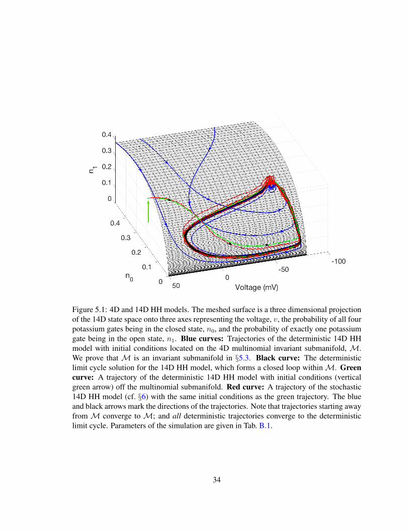
Figure 5.1: 4D and 14D HH models. The meshed surface is a three dimensional projectionof the 14D state space onto three axes representing the voltage, v, the probability of all fourpotassium gates being in the closed state, n0, and the probability of exactly one potassiumgate being in the open state, n1. Blue curves: Trajectories of the deterministic 14D HHmodel with initial conditions located on the 4D multinomial invariant submanifold, M.We prove that M is an invariant submanifold in §5.3. Black curve: The deterministiclimit cycle solution for the 14D HH model, which forms a closed loop withinM. Greencurve: A trajectory of the deterministic 14D HH model with initial conditions (verticalgreen arrow) off the multinomial submanifold. Red curve: A trajectory of the stochastic14D HH model (cf. §6) with the same initial conditions as the green trajectory. The blueand black arrows mark the directions of the trajectories. Note that trajectories starting awayfrom M converge to M; and all deterministic trajectories converge to the deterministiclimit cycle. Parameters of the simulation are given in Tab. B.1.
34
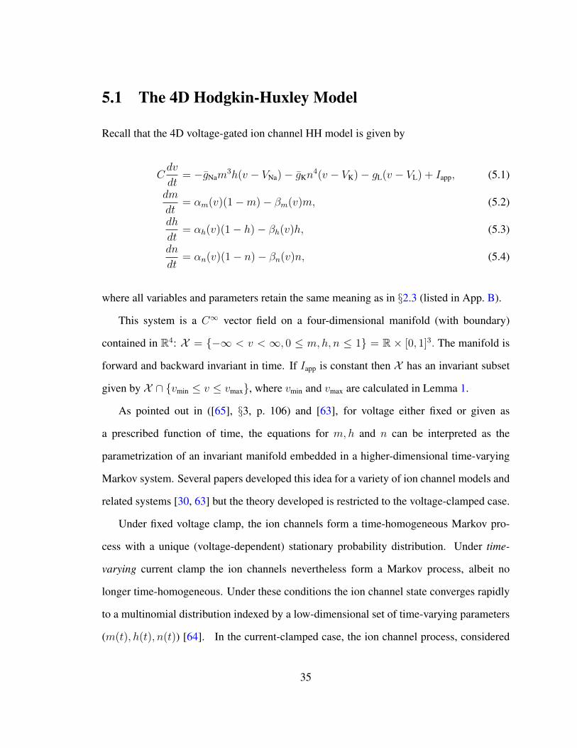
5.1 The 4D Hodgkin-Huxley Model
Recall that the 4D voltage-gated ion channel HH model is given by
Cdv
dt= −gNam
3h(v − VNa)− gKn4(v − VK)− gL(v − VL) + Iapp, (5.1)
dm
dt= αm(v)(1−m)− βm(v)m, (5.2)
dh
dt= αh(v)(1− h)− βh(v)h, (5.3)
dn
dt= αn(v)(1− n)− βn(v)n, (5.4)
where all variables and parameters retain the same meaning as in §2.3 (listed in App. B).
This system is a C∞ vector field on a four-dimensional manifold (with boundary)
contained in R4: X = −∞ < v < ∞, 0 ≤ m,h, n ≤ 1 = R × [0, 1]3. The manifold is
forward and backward invariant in time. If Iapp is constant then X has an invariant subset
given by X ∩ vmin ≤ v ≤ vmax, where vmin and vmax are calculated in Lemma 1.
As pointed out in ([65], §3, p. 106) and [63], for voltage either fixed or given as
a prescribed function of time, the equations for m,h and n can be interpreted as the
parametrization of an invariant manifold embedded in a higher-dimensional time-varying
Markov system. Several papers developed this idea for a variety of ion channel models and
related systems [30, 63] but the theory developed is restricted to the voltage-clamped case.
Under fixed voltage clamp, the ion channels form a time-homogeneous Markov pro-
cess with a unique (voltage-dependent) stationary probability distribution. Under time-
varying current clamp the ion channels nevertheless form a Markov process, albeit no
longer time-homogeneous. Under these conditions the ion channel state converges rapidly
to a multinomial distribution indexed by a low-dimensional set of time-varying parameters
(m(t), h(t), n(t)) [64]. In the current-clamped case, the ion channel process, considered
35
alone, is neither stationary nor Markovian, making the analysis of this case significantly
more challenging, from a mathematical point of view.
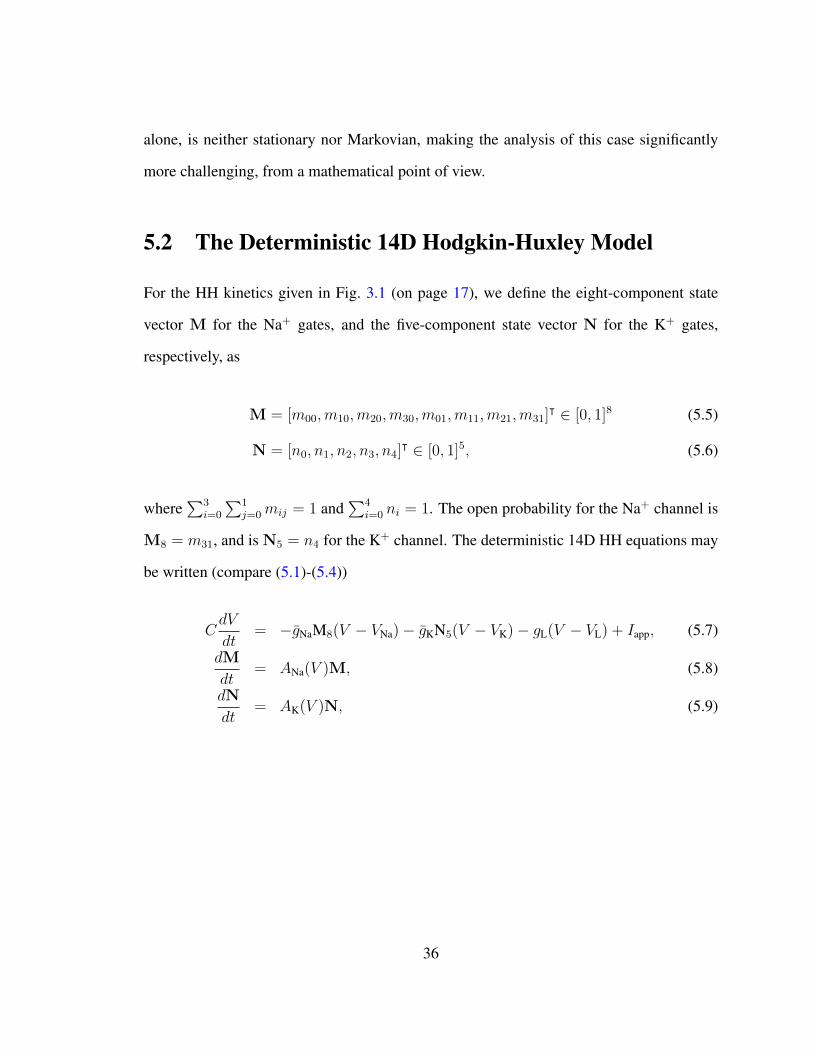
5.2 The Deterministic 14D Hodgkin-Huxley Model
For the HH kinetics given in Fig. 3.1 (on page 17), we define the eight-component state
vector M for the Na+ gates, and the five-component state vector N for the K+ gates,
respectively, as
M = [m00,m10,m20,m30,m01,m11,m21,m31]ᵀ ∈ [0, 1]8 (5.5)
N = [n0, n1, n2, n3, n4]ᵀ ∈ [0, 1]5, (5.6)
where∑3
i=0
∑1j=0mij = 1 and
∑4i=0 ni = 1. The open probability for the Na+ channel is
M8 = m31, and is N5 = n4 for the K+ channel. The deterministic 14D HH equations may
be written (compare (5.1)-(5.4))
CdV
dt= −gNaM8(V − VNa)− gKN5(V − VK)− gL(V − VL) + Iapp, (5.7)
dM
dt= ANa(V )M, (5.8)
dN
dt= AK(V )N, (5.9)
36
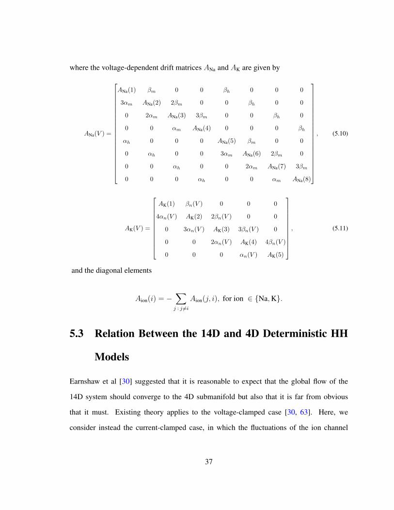
where the voltage-dependent drift matrices ANa and AK are given by
ANa(V ) =
ANa(1) βm 0 0 βh 0 0 0
3αm ANa(2) 2βm 0 0 βh 0 0
0 2αm ANa(3) 3βm 0 0 βh 0
0 0 αm ANa(4) 0 0 0 βh
αh 0 0 0 ANa(5) βm 0 0
0 αh 0 0 3αm ANa(6) 2βm 0
0 0 αh 0 0 2αm ANa(7) 3βm
0 0 0 αh 0 0 αm ANa(8)
, (5.10)
AK(V ) =
AK(1) βn(V ) 0 0 0
4αn(V ) AK(2) 2βn(V ) 0 0
0 3αn(V ) AK(3) 3βn(V ) 0
0 0 2αn(V ) AK(4) 4βn(V )
0 0 0 αn(V ) AK(5)
, (5.11)
and the diagonal elements
Aion(i) = −∑j : j 6=i
Aion(j, i), for ion ∈ Na,K.
5.3 Relation Between the 14D and 4D Deterministic HH
Models
Earnshaw et al [30] suggested that it is reasonable to expect that the global flow of the
14D system should converge to the 4D submanifold but also that it is far from obvious
that it must. Existing theory applies to the voltage-clamped case [30, 63]. Here, we
consider instead the current-clamped case, in which the fluctuations of the ion channel
37
state influences the voltage evolution, and vice-versa.
In the remainder of this section we will (1) define a multinomial submanifold M and
show that it is an invariant manifold within the 14D space, and (2) show that the velocity
on the 14D space and the pushforward of the velocity on the 4D space are identical. In §5.4
we will (3) provide numerical evidence that M is globally attracting within the higher-
dimensional space.
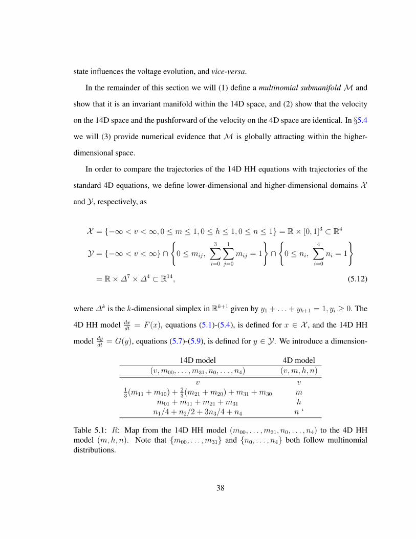
In order to compare the trajectories of the 14D HH equations with trajectories of the
standard 4D equations, we define lower-dimensional and higher-dimensional domains X
and Y , respectively, as
X = −∞ < v <∞, 0 ≤ m ≤ 1, 0 ≤ h ≤ 1, 0 ≤ n ≤ 1 = R× [0, 1]3 ⊂ R4
Y = −∞ < v <∞ ∩
0 ≤ mij,
3∑i=0
1∑j=0
mij = 1
∩
0 ≤ ni,
4∑i=0
ni = 1
= R×∆7 ×∆4 ⊂ R14, (5.12)
where ∆k is the k-dimensional simplex in Rk+1 given by y1 + . . .+ yk+1 = 1, yi ≥ 0. The
4D HH model dxdt
= F (x), equations (5.1)-(5.4), is defined for x ∈ X , and the 14D HH
model dydt
= G(y), equations (5.7)-(5.9), is defined for y ∈ Y . We introduce a dimension-
14D model 4D model(v,m00, . . . ,m31, n0, . . . , n4) (v,m, h, n)
v v13(m11 +m10) + 2
3(m21 +m20) +m31 +m30 m
m01 +m11 +m21 +m31 hn1/4 + n2/2 + 3n3/4 + n4 n ‘
Table 5.1: R: Map from the 14D HH model (m00, . . . ,m31, n0, . . . , n4) to the 4D HHmodel (m,h, n). Note that m00, . . . ,m31 and n0, . . . , n4 both follow multinomialdistributions.
38
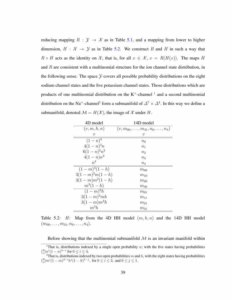
reducing mapping R : Y → X as in Table 5.1, and a mapping from lower to higher
dimension, H : X → Y as in Table 5.2. We construct R and H in such a way that
R H acts as the identity on X , that is, for all x ∈ X , x = R(H(x)). The maps H
and R are consistent with a multinomial structure for the ion channel state distribution, in
the following sense. The space Y covers all possible probability distributions on the eight
sodium channel states and the five potassium channel states. Those distributions which are
products of one multinomial distribution on the K+-channel 1 and a second multinomial
distribution on the Na+-channel2 form a submanifold of ∆7 ×∆4. In this way we define a
submanifold, denotedM = H(X ), the image of X under H .
4D model 14D model(v,m, h, n) (v,m00, . . . ,m31, n0, . . . , n4)
v v
(1− n)4 n0
4(1− n)3n n1
6(1− n)2n2 n2
4(1− n)n3 n3
n4 n4
(1−m)3(1− h) m00
3(1−m)2m(1− h) m10
3(1−m)m2(1− h) m20
m3(1− h) m30
(1−m)3h m01
3(1−m)2mh m11
3(1−m)m2h m21
m3h m31
Table 5.2: H: Map from the 4D HH model (m,h, n) and the 14D HH model(m00, . . . ,m31, n0, . . . , n4).
Before showing that the multinomial submanifold M is an invariant manifold within
1That is, distributions indexed by a single open probability n; with the five states having probabilities(4i
)ni(1− n)4−i for 0 ≤ i ≤ 4.2That is, distributions indexed by two open probabilitiesm and h, with the eight states having probabilities(
3i
)mi(1−m)3−ihj(1− h)1−j , for 0 ≤ i ≤ 3, and 0 ≤ j ≤ 1.
39
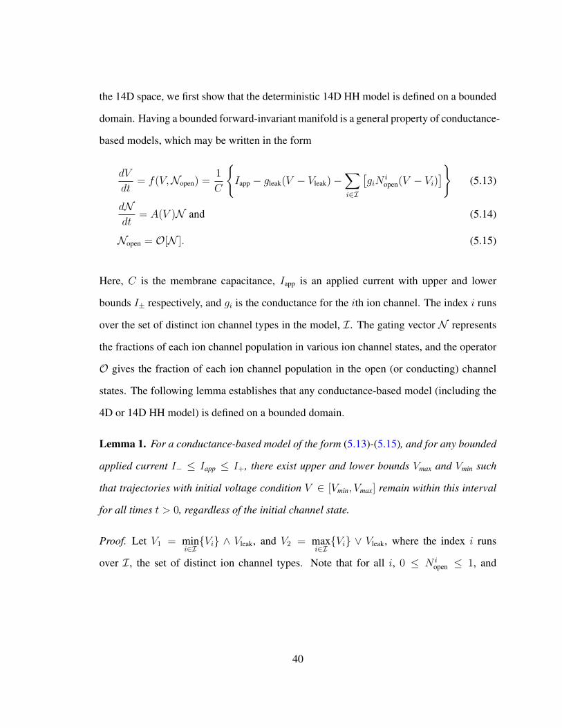
the 14D space, we first show that the deterministic 14D HH model is defined on a bounded
domain. Having a bounded forward-invariant manifold is a general property of conductance-
based models, which may be written in the form
dV
dt= f(V,Nopen) =
1
C
Iapp − gleak(V − Vleak)−
∑i∈I
[giN
iopen(V − Vi)
](5.13)
dNdt
= A(V )N and (5.14)
Nopen = O[N ]. (5.15)
Here, C is the membrane capacitance, Iapp is an applied current with upper and lower
bounds I± respectively, and gi is the conductance for the ith ion channel. The index i runs
over the set of distinct ion channel types in the model, I. The gating vector N represents
the fractions of each ion channel population in various ion channel states, and the operator
O gives the fraction of each ion channel population in the open (or conducting) channel
states. The following lemma establishes that any conductance-based model (including the
4D or 14D HH model) is defined on a bounded domain.
Lemma 1. For a conductance-based model of the form (5.13)-(5.15), and for any bounded
applied current I− ≤ Iapp ≤ I+, there exist upper and lower bounds Vmax and Vmin such
that trajectories with initial voltage condition V ∈ [Vmin, Vmax] remain within this interval
for all times t > 0, regardless of the initial channel state.
Proof. Let V1 = mini∈IVi ∧ Vleak, and V2 = max
i∈IVi ∨ Vleak, where the index i runs
over I, the set of distinct ion channel types. Note that for all i, 0 ≤ N iopen ≤ 1, and
40
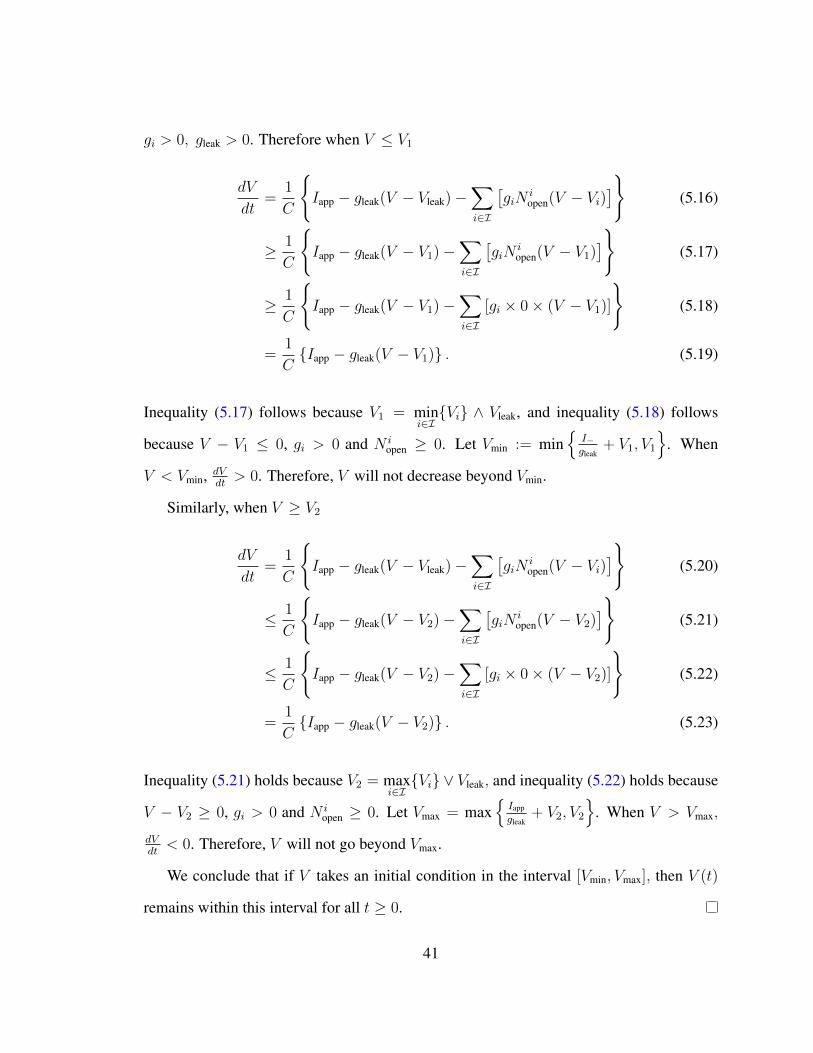
gi > 0, gleak > 0. Therefore when V ≤ V1
dV
dt=
1
C
Iapp − gleak(V − Vleak)−
∑i∈I
[giN
iopen(V − Vi)
](5.16)
≥ 1
C
Iapp − gleak(V − V1)−
∑i∈I
[giN
iopen(V − V1)
](5.17)
≥ 1
C
Iapp − gleak(V − V1)−
∑i∈I
[gi × 0× (V − V1)]
(5.18)
=1
CIapp − gleak(V − V1) . (5.19)
Inequality (5.17) follows because V1 = mini∈IVi ∧ Vleak, and inequality (5.18) follows
because V − V1 ≤ 0, gi > 0 and N iopen ≥ 0. Let Vmin := min
I−gleak
+ V1, V1
. When
V < Vmin, dVdt> 0. Therefore, V will not decrease beyond Vmin.
Similarly, when V ≥ V2
dV
dt=
1
C
Iapp − gleak(V − Vleak)−
∑i∈I
[giN
iopen(V − Vi)
](5.20)
≤ 1
C
Iapp − gleak(V − V2)−
∑i∈I
[giN
iopen(V − V2)
](5.21)
≤ 1
C
Iapp − gleak(V − V2)−
∑i∈I
[gi × 0× (V − V2)]
(5.22)
=1
CIapp − gleak(V − V2) . (5.23)
Inequality (5.21) holds because V2 = maxi∈IVi ∨ Vleak, and inequality (5.22) holds because
V − V2 ≥ 0, gi > 0 and N iopen ≥ 0. Let Vmax = max
Iapp
gleak+ V2, V2
. When V > Vmax,
dVdt< 0. Therefore, V will not go beyond Vmax.
We conclude that if V takes an initial condition in the interval [Vmin, Vmax], then V (t)
remains within this interval for all t ≥ 0.
41
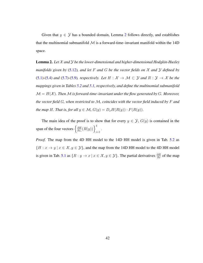
Given that y ∈ Y has a bounded domain, Lemma 2 follows directly, and establishes
that the multinomial submanifoldM is a forward-time–invariant manifold within the 14D
space.
Lemma 2. LetX andY be the lower-dimensional and higher-dimensional Hodgkin-Huxley
manifolds given by (5.12), and let F and G be the vector fields on X and Y defined by
(5.1)-(5.4) and (5.7)-(5.9), respectively. Let H : X → M ⊂ Y and R : Y → X be the
mappings given in Tables 5.2 and 5.1, respectively, and define the multinomial submanifold
M = H(X ). ThenM is forward-time–invariant under the flow generated byG. Moreover,
the vector field G, when restricted toM, coincides with the vector field induced by F and
the map H . That is, for all y ∈M, G(y) = DxH(R(y)) · F (R(y)).
The main idea of the proof is to show that for every y ∈ Y , G(y) is contained in the
span of the four vectors∂H∂xi
(R(y))4
i=1.
Proof. The map from the 4D HH model to the 14D HH model is given in Tab. 5.2 as
H : x → y | x ∈ X , y ∈ Y, and the map from the 14D HH model to the 4D HH model
is given in Tab. 5.1 as R : y → x | x ∈ X , y ∈ Y. The partial derivatives ∂H∂x
of the map
42
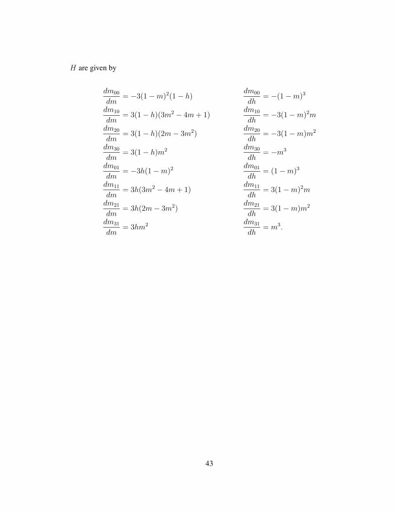
H are given by
dm00
dm= −3(1−m)2(1− h)
dm00
dh= −(1−m)3
dm10
dm= 3(1− h)(3m2 − 4m+ 1)
dm10
dh= −3(1−m)2m
dm20
dm= 3(1− h)(2m− 3m2)
dm20
dh= −3(1−m)m2
dm30
dm= 3(1− h)m2 dm30
dh= −m3
dm01
dm= −3h(1−m)2
dm01
dh= (1−m)3
dm11
dm= 3h(3m2 − 4m+ 1)
dm11
dh= 3(1−m)2m
dm21
dm= 3h(2m− 3m2)
dm21
dh= 3(1−m)m2
dm31
dm= 3hm2 dm31
dh= m3.
43
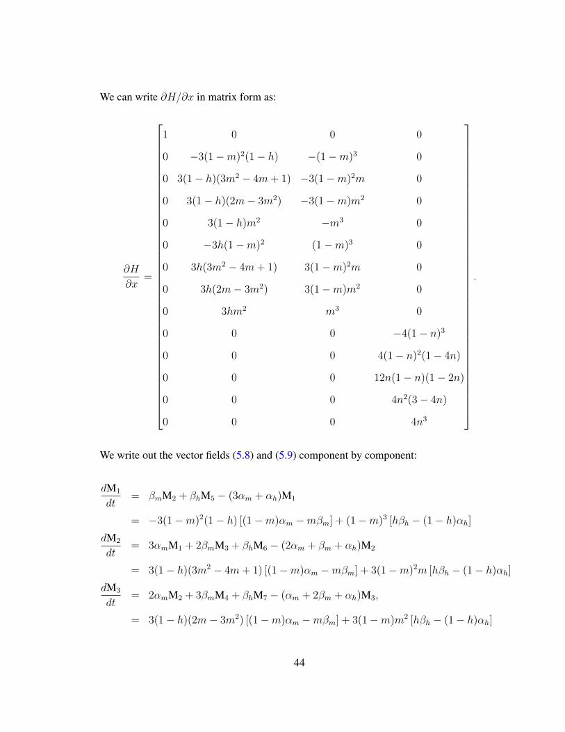
We can write ∂H/∂x in matrix form as:
∂H
∂x=
1 0 0 0
0 −3(1−m)2(1− h) −(1−m)3 0
0 3(1− h)(3m2 − 4m+ 1) −3(1−m)2m 0
0 3(1− h)(2m− 3m2) −3(1−m)m2 0
0 3(1− h)m2 −m3 0
0 −3h(1−m)2 (1−m)3 0
0 3h(3m2 − 4m+ 1) 3(1−m)2m 0
0 3h(2m− 3m2) 3(1−m)m2 0
0 3hm2 m3 0
0 0 0 −4(1− n)3
0 0 0 4(1− n)2(1− 4n)
0 0 0 12n(1− n)(1− 2n)
0 0 0 4n2(3− 4n)
0 0 0 4n3
.
We write out the vector fields (5.8) and (5.9) component by component:
dM1
dt= βmM2 + βhM5 − (3αm + αh)M1
= −3(1−m)2(1− h) [(1−m)αm −mβm] + (1−m)3 [hβh − (1− h)αh]
dM2
dt= 3αmM1 + 2βmM3 + βhM6 − (2αm + βm + αh)M2
= 3(1− h)(3m2 − 4m+ 1) [(1−m)αm −mβm] + 3(1−m)2m [hβh − (1− h)αh]
dM3
dt= 2αmM2 + 3βmM4 + βhM7 − (αm + 2βm + αh)M3,
= 3(1− h)(2m− 3m2) [(1−m)αm −mβm] + 3(1−m)m2 [hβh − (1− h)αh]
44
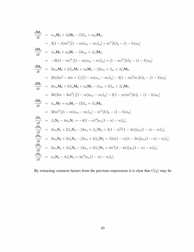
dM4
dt= αmM3 + βhM8 − (3βm + αh)M4,
= 3(1− h)m2 [(1−m)αm −mβm] +m3 [hβh − (1− h)αh]
dM5
dt= βmM6 + αhM1 − (3αm + βh)M5,
= −3h(1−m)2 [(1−m)αm −mβm] + (1−m)3 [hβh − (1− h)αh]
dM6
dt= 3αmM5 + 2βmM7 + αhM2 − (2αm + βm + βh)M6,
= 3h(3m2 − 4m+ 1) [(1−m)αm −mβm]− 3(1−m)2m [hβh − (1− h)αh]
dM7
dt= 2αmM6 + 3βmM8 + αhM3 − (αm + 2βm + βh)M7,
= 3h(2m− 3m2) [(1−m)αm −mβm]− 3(1−m)m2 [hβh − (1− h)αh]
dM8
dt= αmM7 + αhM4 − (3βm + βh)M8,
= 3hm2 [(1−m)αm −mβm]−m3 [hβh − (1− h)αh]
dN1
dt= βnN2 − 4αnN1 = −4(1− n)3[αn(1− n)− nβn],
dN2
dt= 4αnN1 + 2βnN3 − (3αn + βn)N2 = 4(1− n)2(1− 4n)[αn(1− n)− nβn],
dN3
dt= 3αnN2 + 3βnN4 − (2αn + 2βn)N3 = 12n(1− n)(1− 2n)[αn(1− n)− nβn],
dN4
dt= 2αnN3 + 4βnN5 − (3αn + 3βn)N4 = 4n2(3− 4n)[αn(1− n)− nβn],
dN5
dt= αnN4 − 4βnN5 = 4n3[αn(1− n)− nβn].
By extracting common factors from the previous expressions it is clear that G(y) may be
45
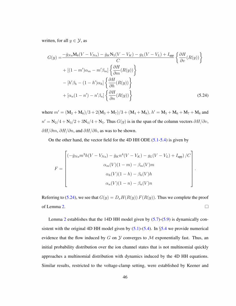
written, for all y ∈ Y , as
G(y) =−gNaM8(V − VNa)− gKN5(V − VK)− gL(V − VL) + Iapp
C
∂H
∂v(R(y))
+ [(1−m′)αm −m′βm]
∂H
∂m(R(y))
− [h′βh − (1− h′)αh]
∂H
∂h(R(y))
+ [αn(1− n′)− n′βn]
∂H
∂n(R(y))
(5.24)
where m′ = (M2 + M6)/3 + 2(M3 + M7)/3 + (M4 + M8), h′ = M5 + M6 + M7 + M8 and
n′ = N2/4 + N3/2 + 3N4/4 + N5. Thus G(y) is in the span of the column vectors ∂H/∂v,
∂H/∂m, ∂H/∂n, and ∂H/∂h, as was to be shown.
On the other hand, the vector field for the 4D HH ODE (5.1-5.4) is given by
F =
(−gNam3h(V − VNa)− gKn4(V − VK)− gL(V − VL) + Iapp) /C
αm(V )(1−m)− βm(V )m
αh(V )(1− h)− βh(V )h
αn(V )(1− n)− βn(V )n
.
Referring to (5.24), we see thatG(y) = DxH(R(y))F (R(y)). Thus we complete the proof
of Lemma 2.
Lemma 2 establishes that the 14D HH model given by (5.7)-(5.9) is dynamically con-
sistent with the original 4D HH model given by (5.1)-(5.4). In §5.4 we provide numerical
evidence that the flow induced by G on Y converges to M exponentially fast. Thus, an
initial probability distribution over the ion channel states that is not multinomial quickly
approaches a multinomial distribution with dynamics induced by the 4D HH equations.
Similar results, restricted to the voltage-clamp setting, were established by Keener and
46
Earnshaw [30, 63, 65].
5.4 Local Convergence Rate
Keener and Earnshaw [30, 63, 65] showed that for Markov chains with constant (even
time varying) transition rates: (i) the multinomial probability distributions corresponding
to mean-field models (such as the HH sodium or potassium models) form invariant sub-
manifolds within the space of probability distributions over the channel states, and (ii)
arbitrary initial probability distributions converged exponentially quickly to the invariant
manifold. For systems with prescribed time-varying transition rates, such as for an ion
channel system under voltage clamp with a prescribed voltage V (t) as a function of time,
the distribution of channel states had an invariant submanifold again corresponding to the
multinomial distributions, and the flow on that manifold induced by the evolution equations
was consistent with the flow of the full system.
In the preceding section we established the dynamical consistency of the 14D and 4D
models with enough generality to cover both the voltage-clamp and current-clamp systems;
the latter is distinguished by NOT having a prescribed voltage trace, but rather having
the voltage coevolve along with the (randomly fluctuating) ion channel states. Here, we
give numerical evidence for exponential convergence under current clamp similar to that
established under voltage clamp by Keener and Earnshaw.
Rather than providing a rigorous proof, we give numerical evidence for the standard
deterministic HH model that y →M under current clamp (spontaneous firing conditions)
in the following sense: if y(t) is a solution of y = G(y) with arbitrary initial data y0 ∈
Y , then ||y(t) − H(R(y(t)))|| → 0 as t → ∞, exponentially quickly. Moreover, the
convergence rate is bounded by λ = max(λv, λNa, λK), where λion is the least negative
47
nontrivial eigenvalue of the channel state transition matrix (over the voltage range Vmin ≤
v ≤ Vmax) for a given ion, and −1/λv is the largest value taken by the membrane time
constant (for Vmin ≤ v ≤ Vmax). In practice, we find that the membrane time constant
does not determine the slowest time scale for convergence toM. In fact it appears that the
second-least-negative eigenvalues (not the least-negative eigenvalues) of the ion channel
matrices set the convergence rate.
Note that y ∈ Y can be written as y = [V ;M;N]. The Jacobian matrix ∂H∂x
consists of
three block matrices: one for the voltage terms, ∂V∂v
, one associated to the Na+ gates, given
by ∂M∂m
and ∂M∂h
, and one corresponding to the K+ gates, ∂N∂n
. Fixing a particular voltage
v, let λi, i ∈ 0, 1, 2, . . . , 7 be the eight eigenvalues of ANa and vi be the associated
eigenvectors, i.e., ANavi = λivi for the rate matrix in equations (5.8). Similarly, let
ηi, wi, i ∈ 0, 1, 2, . . . , 4 be the five eigenvalues and the associated eigenvectors of AK,
i.e.,AKwi = ηiwi, for the rate matrix in equations (5.9). If we rank the eigenvalues of either
matrix in descending order, the leading eigenvalue is always zero (because the sum of each
column for ANa and AK is zero for every V ) and the remainder are real and negative. Let λ1
and η1 denote the largest (least negative) nontrivial eigenvalues ofANa andAK, respectively,
and let v1 ∈ R8 and w1 ∈ R5 be the corresponding eigenvectors.
The eigenvectors of the full 14D Jacobian are not simply related to the eigenvectors of
the component submatrices, because the first (voltage) row and column contain nonzero off-
diagonal elements. However, the eigenvectors associated to the largest nonzero eigenvec-
tors of ANa and AK (respectively v2 and w2) are parallel to ∂M/∂h and ∂N/∂n, regardless
of voltage. In other words, the slowest decaying directions for each ion channel, v1 and w1,
transport the flow along the multinominal sub-manifold of Y . Therefore, it is reasonable to
make the hypothesis that if Y (t) is a solution of y = G(y) with arbitrary initial data y ∈ Y ,
48
then||y(t)−H(R(y(t)))||||y(0)−H(R(y(0)))||
. e−λ2t (5.25)
for λ2 being the second largest nonzero eigenvalue of AK and ANa over all v in the range
vmin < v < vmax. The convergence behavior is plotted numerically in Fig. 5.2, and is
consistent with the Ansatz (5.25). We calculate the distance from a point y toM as
ymax = argmaxy∈Y
‖y −H(R(y))‖2 . (5.26)
In order to obtain an upper bound on the distance as a function of time, we begin with the
furthest point in the simplex fromM, by numerically finding the solution to the argument
(5.26), which is
ymax = [v, 0.5, 0, 0, 0.5, 0, 0, 0, 0, 0.5, 0, 0, 0, 0.5].
This vector represents the furthest possible departure from the multinomial distribution:
all probability equally divided between the extreme states m00 and m03 for the sodium
channel, and the extremal states n0 and n4 for potassium. The maximum distance from the
multinomial submanifold M, dmax, is calculated using this point. As shown in Fig. 5.2,
the function dmax e−λ2t provides a tight upper bound for the convergence rate from arbitrary
initial data y ∈ Y to the invariant submanifoldM.
49
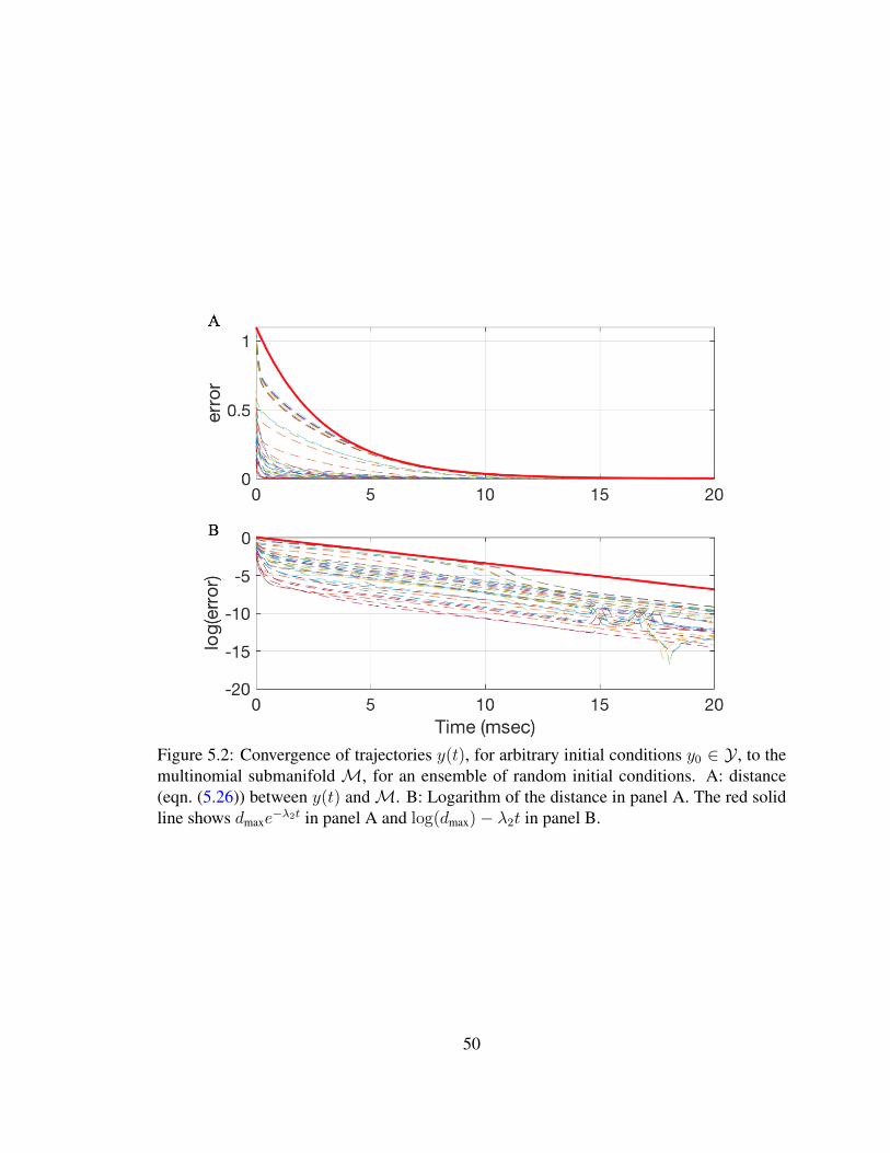
Figure 5.2: Convergence of trajectories y(t), for arbitrary initial conditions y0 ∈ Y , to themultinomial submanifold M, for an ensemble of random initial conditions. A: distance(eqn. (5.26)) between y(t) andM. B: Logarithm of the distance in panel A. The red solidline shows dmaxe
−λ2t in panel A and log(dmax)− λ2t in panel B.
50
Chapter 6
Stochastic 14D Hodgkin-Huxley Models
Finite populations of ion channels generate stochastic fluctuations (“channel noise”) in
ionic currents that influence action potential initiation and timing [107, 125]. At the molec-
ular level, fluctuations arise because transitions between individual ion channel states are
stochastic [58, 85, 116]. Each directed edge in the ion channel state transition diagrams
(cf. Fig. 3.1) introduces an independent noise source. It is of interest to be able to attribute
variability of the interspike interval timing distribution to specific molecular noise sources,
specifically individual directed edges in each channel state graph. In order to explore
these contributions, we develop a system of Langevin equations for the Hodgkin-Huxley
equations, set in a 14-dimensional phase space.
Working with a higher-dimensional stochastic model may appear inconvenient, but
in fact has several advantages. First, any projection of an underlying 14D model onto a
lower (e.g. 4D) stochastic model generally entails loss of the Markov property. Second, the
higher-dimensional representation allows us to assess the contribution of individual molec-
ular transitions to the macroscopically observable variability of timing in the interspike
51
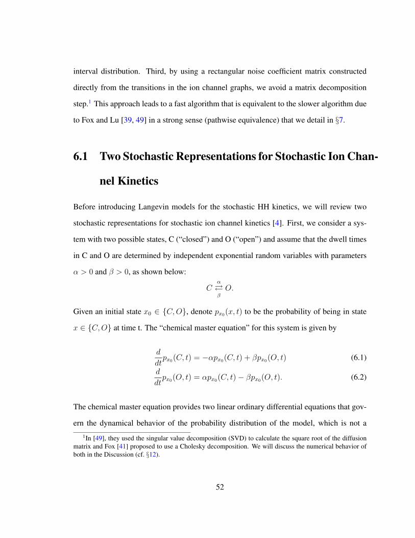
interval distribution. Third, by using a rectangular noise coefficient matrix constructed
directly from the transitions in the ion channel graphs, we avoid a matrix decomposition
step.1 This approach leads to a fast algorithm that is equivalent to the slower algorithm due
to Fox and Lu [39, 49] in a strong sense (pathwise equivalence) that we detail in §7.
6.1 Two Stochastic Representations for Stochastic Ion Chan-
nel Kinetics
Before introducing Langevin models for the stochastic HH kinetics, we will review two
stochastic representations for stochastic ion channel kinetics [4]. First, we consider a sys-
tem with two possible states, C (“closed”) and O (“open”) and assume that the dwell times
in C and O are determined by independent exponential random variables with parameters
α > 0 and β > 0, as shown below:
Cα
βO.
Given an initial state x0 ∈ C,O, denote px0(x, t) to be the probability of being in state
x ∈ C,O at time t. The “chemical master equation” for this system is given by
d
dtpx0(C, t) = −αpx0(C, t) + βpx0(O, t) (6.1)
d
dtpx0(O, t) = αpx0(C, t)− βpx0(O, t). (6.2)
The chemical master equation provides two linear ordinary differential equations that gov-
ern the dynamical behavior of the probability distribution of the model, which is not a
1In [49], they used the singular value decomposition (SVD) to calculate the square root of the diffusionmatrix and Fox [41] proposed to use a Cholesky decomposition. We will discuss the numerical behavior ofboth in the Discussion (cf. §12).
52
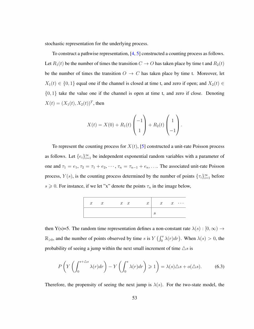
stochastic representation for the underlying process.
To construct a pathwise representation, [4, 5] constructed a counting process as follows.
Let R1(t) be the number of times the transition C → O has taken place by time t and R2(t)
be the number of times the transition O → C has taken place by time t. Moreover, let
X1(t) ∈ 0, 1 equal one if the channel is closed at time t, and zero if open; and X2(t) ∈
0, 1 take the value one if the channel is open at time t, and zero if close. Denoting
X(t) = (X1(t), X2(t))T , then
X(t) = X(0) +R1(t)
−1
1
+R2(t)
1
−1
.
To represent the counting process for X(t), [5] constructed a unit-rate Poisson process
as follows. Let ei∞i=1 be independent exponential random variables with a parameter of
one and τ1 = e1, τ2 = τ1 + e2, · · · , τn = τn−1 + en, . . .. The associated unit-rate Poisson
process, Y (s), is the counting process determined by the number of points τi∞i=1 before
s > 0. For instance, if we let ”x” denote the points τn in the image below,
x x x x x x x · · ·
s
then Y(s)=5. The random time representation defines a non-constant rate λ(s) : [0,∞) →
R>0, and the number of points observed by time s is Y(∫ s
0λ(r)dr
). When λ(s) > 0, the
probability of seeing a jump within the next small increment of time4s is
P
(Y
(∫ s+4s
0
λ(r)dr
)− Y
(∫ s
0
λ(r)dr
)> 1
)= λ(s)4s+ o(4s). (6.3)
Therefore, the propensity of seeing the next jump is λ(s). For the two-state model, the
53
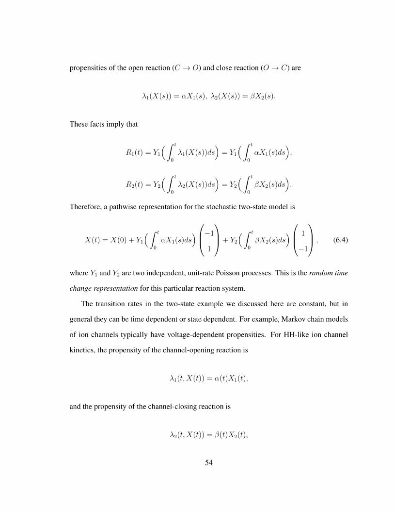
propensities of the open reaction (C → O) and close reaction (O → C) are
λ1(X(s)) = αX1(s), λ2(X(s)) = βX2(s).
These facts imply that
R1(t) = Y1
(∫ t
0
λ1(X(s))ds)
= Y1
(∫ t
0
αX1(s)ds),
R2(t) = Y2
(∫ t
0
λ2(X(s))ds)
= Y2
(∫ t
0
βX2(s)ds).
Therefore, a pathwise representation for the stochastic two-state model is
X(t) = X(0) + Y1
(∫ t
0
αX1(s)ds)−1
1
+ Y2
(∫ t
0
βX2(s)ds) 1
−1
, (6.4)
where Y1 and Y2 are two independent, unit-rate Poisson processes. This is the random time
change representation for this particular reaction system.
The transition rates in the two-state example we discussed here are constant, but in
general they can be time dependent or state dependent. For example, Markov chain models
of ion channels typically have voltage-dependent propensities. For HH-like ion channel
kinetics, the propensity of the channel-opening reaction is
λ1(t,X(t)) = α(t)X1(t),
and the propensity of the channel-closing reaction is
λ2(t,X(t)) = β(t)X2(t),
54
where α(t), and β(t) are voltage-dependent non-negative functions. The analogous expres-
sion for the pathwise representation [4] can be expressed as
X(t) =X(0) + Y1
(∫ t
0
α(s)X1(s)ds)−1
1
+ Y2
(∫ t
0
β(s)X2(s)ds) 1
−1
. (6.5)
As a generalization, [4] extended the random time change representation to a d-state
model with M reaction channels. Denote Xi(t) to be the value of the ith component at time
t, with X(t) ∈ Zd and the propensity of the kth reaction being λk(t,X(t)). If we further
assume that the system is updated immediately once the kth reaction happens at time t
according to the reaction vector ζk ∈ Zd, then
X(t) = X(t−) + ζk.
Thus, the expression for the pathwise representation is
X(t) = X(0) +∑k
Yk
(∫ t
0
λk(t,X(t))ds
)ζk, (6.6)
where the Yk are independent unit-rate Poisson processes.
Algorithm for the simulation of the random time change representation The time
until the next reaction occurs after time T is given by
4 = mink
4k :
∫ T+4k
0
λk(s,X(s))ds = τ kT
,
55
where τ kT is the first point associated with Yk coming after∫ T0λk(s,X(s))ds, which is
defined as follows
τ kT ≡ infr >
∫ T
0
λk(s,X(s))ds : Yk(r)− Yk(∫ T
0
λk(s,X(s))ds
)= 1
.
For a single ion channel type with state variable X, and including the membrane potential
V as an additional dynamical variable, then its pathwise representation is given by
CdV
dt= Iapp(t)− IV (V (t))−
( d∑i=1
goiXi(t))
(V (t)− VX). (6.7)
Here goi is the conductance of an individual channel when it is in the ith state (of channel
X) and the sum gives the total conductance associated with the channel represented by the
vector X , and VX is the reversal potential for the ion channel. Meanwhile the channel state
X(t) evolves stochastically according to (6.6).
Algorithm 1. Simulation random time change representation
1. Initialize: set the initial number of molecules of each species, X . Set the initial
voltage value V . Set t = 0. For each k, set τk= 0 and Tk = 0.
2. Generate M independent, uniform(0,1) random numbers rkMk=1, for each k ∈ 1, 2, · · · ,M,
set τk = ln(1/rk)
3. Numerically integrate equation (6.7) forward in time until one of the following equal-
ities hold: ∫ t+4
t
λk(V (s), X(s))ds = τk − Tk. (6.8)
4. Let µ be the index of the reaction channel where the equality (6.8) holds.
56
5. For each k, set
Tk = Tk +
∫ t+4
t
λk(V (s), X(s))ds,
where4 is determined in step 3.
6. Set t = t+4 and X = X + ζµ
7. Let r be uniform(0,1) and set τµ = τµ + ln(1/r).
8. Return to step 3 or stop.
Gillespie’s algorithm A more widely used algorithm for simulating the stochastic ion
channel kinetics is the Gillespie’s algorithm [16, 46], which is a time-homogeneous method.
For simulating the same system for a multi-state single ion channel kinetics in equa-
tion (6.7), the Gillespie’s algorithm can be presented as follows. Let Y be a unit rate
Poisson process, and ξi, i = 0, 1, 2, . . . be independent, uniform (0, 1) random variables
that are independent of Y . If we define
λ0 (V (s), X(s)) =M∑k=1
λk (V (s), X(s)) , (6.9)
qk(s) =1
λ0 (V (s), X(s))
k∑l=1
λl (V (s), X(s)) , (6.10)
57
where q0 = 0 and k ∈ 1, 2, . . . ,M. The representation for the “Gillespie algorithm” for
the stochastic process of X and V can be written as
R0(t) = Y
(∫ t
0
λ0 (V (s), X(s)) ds
)(6.11)
X(t) = X(0) +M∑k=1
ξk
∫ t
0
1ξR0(s−) ∈ [qk−1(s−), qk(s−)]dR0(s) (6.12)
CdV
dt= Iapp(t)− IV (V (t))−
( d∑i=1
goiXi(t))
(V (t)− VX). (6.13)
The corresponding algorithm is given by
Algorithm 2. The Gillespie’s algorithm
1. Initialize: set the initial number of molecules of each species, X . Set a initial voltage
value V and t = 0.
2. Let r be uniform(0,1) and numerically integrate equation (6.11) forward in time until:∫ t+4t
λ0(V (s), X(s))ds = ln(1/r).
3. Let ξ be uniform(0,1) and find the index k where ξ ∈ [qk−1((t+4)−), qk((t+4)−)]
4. Set t = t+4 and X = X + ζk
5. Return to step 2 or stop
6.2 Exact Stochastic Simulation of HH Kinetics: the Random–
Time-Change Representation
An “exact” representation of the Hodgkin-Huxley system with a population of Mtot sodium
channels and Ntot potassium channels treats each of the 20 directed edges in the sodium
58
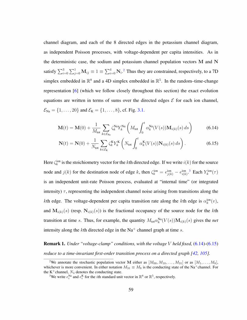
channel diagram, and each of the 8 directed edges in the potassium channel diagram,
as independent Poisson processes, with voltage-dependent per capita intensities. As in
the deterministic case, the sodium and potassium channel population vectors M and N
satisfy∑3
i=0
∑1j=0 Mij ≡ 1 ≡
∑4i=0Ni.2 Thus they are constrained, respectively, to a 7D
simplex embedded in R8 and a 4D simplex embedded in R5. In the random–time-change
representation [6] (which we follow closely throughout this section) the exact evolution
equations are written in terms of sums over the directed edges E for each ion channel,
ENa = 1, . . . , 20 and EK = 1, . . . , 8, cf. Fig. 3.1.
M(t) = M(0) +1
Mtot
∑k∈ENa
ζNak Y
Nak
(Mtot
∫ t
0
αNak (V (s))Mi(k)(s) ds
)(6.14)
N(t) = N(0) +1
Ntot
∑k∈EK
ζKk Y
Kk
(Ntot
∫ t
0
αKk (V (s))Ni(k)(s) ds
). (6.15)
Here ζ ionk is the stoichiometry vector for the kth directed edge. If we write i(k) for the source
node and j(k) for the destination node of edge k, then ζ ionk = eion
j(k) − eioni(k).
3 Each Y ionk (τ)
is an independent unit-rate Poisson process, evaluated at “internal time” (or integrated
intensity) τ , representing the independent channel noise arising from transitions along the
kth edge. The voltage-dependent per capita transition rate along the kth edge is αionk (v),
and Mi(k)(s) (resp. Ni(k)(s)) is the fractional occupancy of the source node for the kth
transition at time s. Thus, for example, the quantity MtotαNak (V (s))Mi(k)(s) gives the net
intensity along the kth directed edge in the Na+ channel graph at time s.
Remark 1. Under “voltage-clamp” conditions, with the voltage V held fixed, (6.14)-(6.15)
reduce to a time-invariant first-order transition process on a directed graph [42, 105].
2We annotate the stochastic population vector M either as [M00,M10, . . . ,M31] or as [M1, . . . ,M8],whichever is more convenient. In either notation M31 ≡ M8 is the conducting state of the Na+channel. Forthe K+channel, N4 denotes the conducting state.
3We write eNai and eK
i for the ith standard unit vector in R8 or R5, respectively.
59
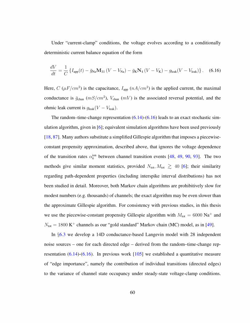
Under “current-clamp” conditions, the voltage evolves according to a conditionally
deterministic current balance equation of the form
dV
dt=
1
CIapp(t)− gNaM31 (V − VNa)− gKN4 (V − VK)− gleak(V − Vleak) . (6.16)
Here, C (µF/cm2) is the capacitance, Iapp (nA/cm2) is the applied current, the maximal
conductance is gchan (mS/cm2), Vchan (mV ) is the associated reversal potential, and the
ohmic leak current is gleak(V − Vleak).
The random–time-change representation (6.14)-(6.16) leads to an exact stochastic sim-
ulation algorithm, given in [6]; equivalent simulation algorithms have been used previously
[18, 87]. Many authors substitute a simplified Gillespie algorithm that imposes a piecewise-
constant propensity approximation, described above, that ignores the voltage dependence
of the transition rates αionk between channel transition events [48, 49, 90, 93]. The two
methods give similar moment statistics, provided Ntot,Mtot & 40 [6]; their similarity
regarding path-dependent properties (including interspike interval distributions) has not
been studied in detail. Moreover, both Markov chain algorithms are prohibitively slow for
modest numbers (e.g. thousands) of channels; the exact algorithm may be even slower than
the approximate Gillespie algorithm. For consistency with previous studies, in this thesis
we use the piecewise-constant propensity Gillespie algorithm with Mtot = 6000 Na+ and
Ntot = 1800 K+ channels as our “gold standard” Markov chain (MC) model, as in [49].
In §6.3 we develop a 14D conductance-based Langevin model with 28 independent
noise sources – one for each directed edge – derived from the random–time-change rep-
resentation (6.14)-(6.16). In previous work [105] we established a quantitative measure
of “edge importance”, namely the contribution of individual transitions (directed edges)
to the variance of channel state occupancy under steady-state voltage-clamp conditions.
60
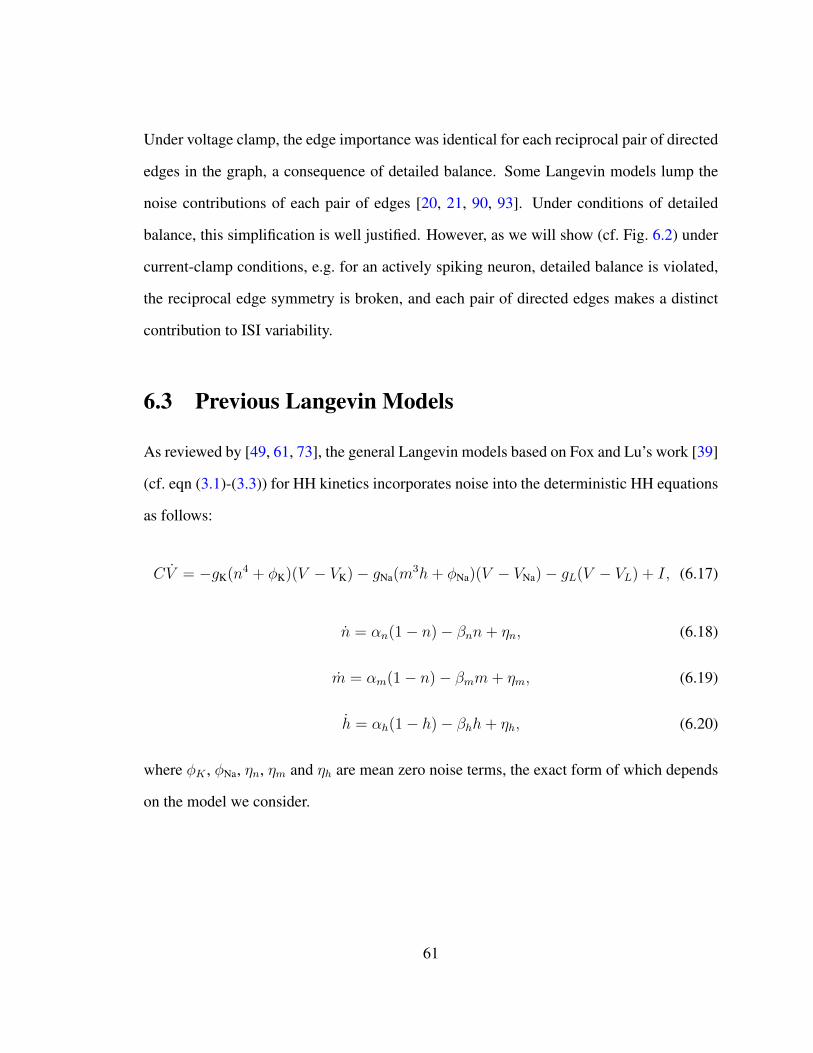
Under voltage clamp, the edge importance was identical for each reciprocal pair of directed
edges in the graph, a consequence of detailed balance. Some Langevin models lump the
noise contributions of each pair of edges [20, 21, 90, 93]. Under conditions of detailed
balance, this simplification is well justified. However, as we will show (cf. Fig. 6.2) under
current-clamp conditions, e.g. for an actively spiking neuron, detailed balance is violated,
the reciprocal edge symmetry is broken, and each pair of directed edges makes a distinct
contribution to ISI variability.
6.3 Previous Langevin Models
As reviewed by [49, 61, 73], the general Langevin models based on Fox and Lu’s work [39]
(cf. eqn (3.1)-(3.3)) for HH kinetics incorporates noise into the deterministic HH equations
as follows:
CV = −gK(n4 + φK)(V − VK)− gNa(m3h+ φNa)(V − VNa)− gL(V − VL) + I, (6.17)
n = αn(1− n)− βnn+ ηn, (6.18)
m = αm(1− n)− βmm+ ηm, (6.19)
h = αh(1− h)− βhh+ ηh, (6.20)
where φK , φNa, ηn, ηm and ηh are mean zero noise terms, the exact form of which depends
on the model we consider.
61
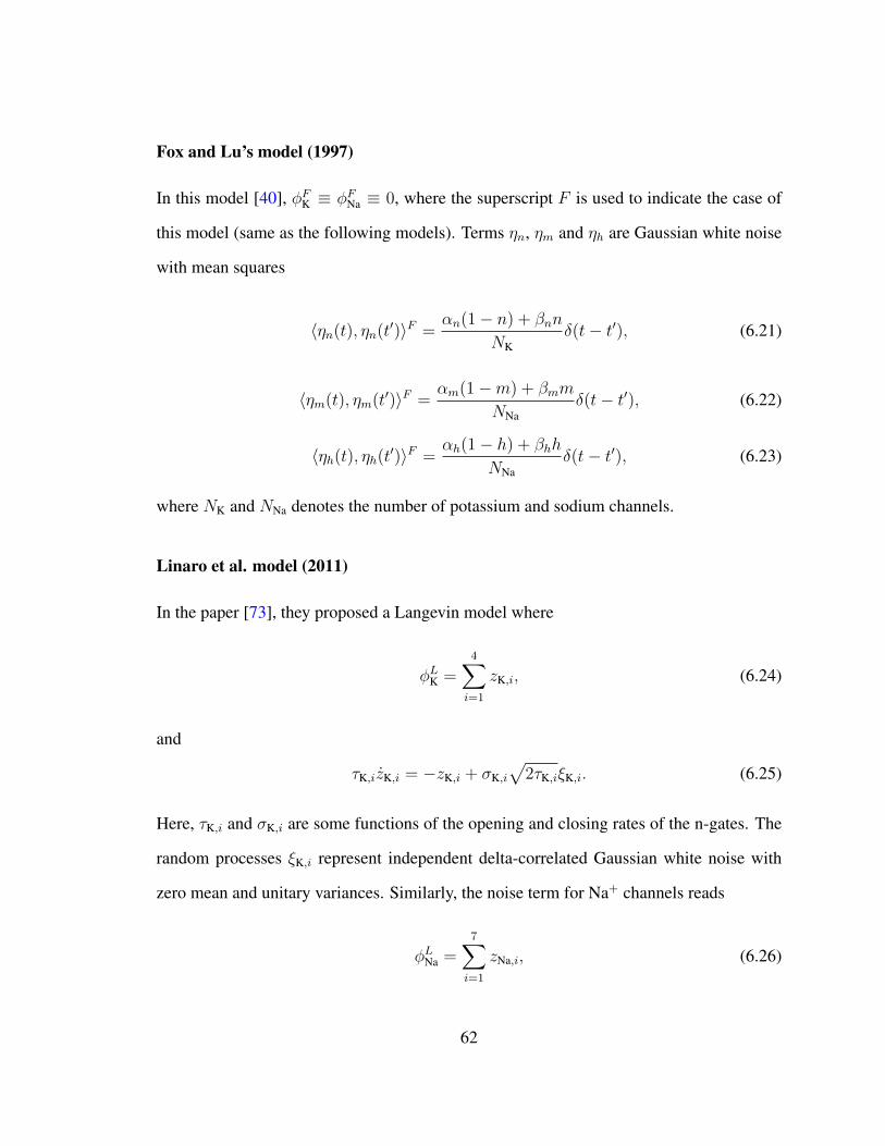
Fox and Lu’s model (1997)
In this model [40], φFK ≡ φFNa ≡ 0, where the superscript F is used to indicate the case of
this model (same as the following models). Terms ηn, ηm and ηh are Gaussian white noise
with mean squares
〈ηn(t), ηn(t′)〉F =αn(1− n) + βnn
NKδ(t− t′), (6.21)
〈ηm(t), ηm(t′)〉F =αm(1−m) + βmm
NNaδ(t− t′), (6.22)
〈ηh(t), ηh(t′)〉F =αh(1− h) + βhh
NNaδ(t− t′), (6.23)
where NK and NNa denotes the number of potassium and sodium channels.
Linaro et al. model (2011)
In the paper [73], they proposed a Langevin model where
φLK =4∑i=1
zK,i, (6.24)
and
τK,izK,i = −zK,i + σK,i√
2τK,iξK,i. (6.25)
Here, τK,i and σK,i are some functions of the opening and closing rates of the n-gates. The
random processes ξK,i represent independent delta-correlated Gaussian white noise with
zero mean and unitary variances. Similarly, the noise term for Na+ channels reads
φLNa =7∑i=1
zNa,i, (6.26)
62
where
τNa,izNa,i = −zNa,i + σNa,i√
2τNa,iξNa,i. (6.27)
Moreover, the noise term for gating variables are zero: ηn ≡ ηm ≡ ηh ≡ 0.
Guler and Marifi’s model (2013)
In [56], the authors mentioned the “nontrivial cross-correlation persistence (NCCP)”, which
they claimed to be the major cause of the elevated excitability and spontaneous firing
in small-size neuronal membranes. The term φGK , which reflects NCCP attributed to the
K+ channels, is given by
φGK =
√n4(1− n4)
NKqK, (6.28)
where
τ qK = pK, (6.29)
τ pK = −γKpK − ω2K[αn(1− n) + βnn]qK + ξK, (6.30)
and ξK is a delta-correlated, mean zero Gaussian white noise term with mean squares
〈ξK(t), ξK(t′)〉G = γKTK[αn(1− n) + βnn]δ(t− t′). (6.31)
In the above equations, τ corresponds to the unit time. The constants are dimensionless
with: γK = 10, ω2K = 150 and TK = 400. Similarly, the term φGNa, which captures NCCP
attributed to the Na+ channels reads
φGNa =
√m3(1−m3)
NNahqNa, (6.32)
63
where
τ qNa = pNa, (6.33)
τ pNa = −γNapNa − ω2Na[αm(1−m) + βmm]qNa + ξNa, (6.34)
with ξNa a mean zero Gaussian white noise term with mean squares
〈ξNa(t), ξNa(t′)〉G = γNaTNa[αm(1−m) + βmm]δ(t− t′). (6.35)
In the above equations, τ corresponds to the unit time. The constants are dimensionless
with: γNa = 10, ω2Na = 200 and TNa = 800.
The subunit noises are Gaussian and their mean squares satisfy
〈ηn(t), ηn(t′)〉F =αn(1− n) + βnn
4NKδ(t− t′), (6.36)
〈ηm(t), ηm(t′)〉F =αm(1−m) + βmm
3NNaδ(t− t′), (6.37)
〈ηh(t), ηh(t′)〉F =αh(1− h) + βhh
NNaδ(t− t′), (6.38)
where NK and NNa denote the number of potassium and sodium channels.
Orio and Soudry’s Model (2012)
In [90], Orio and Soudry derived the SDE explicitly for HH type ion channel kinetic. They
examined a specific population of N ion channels with M states, where the transition rate
of a single channel from state j to i is given by Aji. In addition, they define the matrix A
to be composed of Aij terms for all i 6= j, and Aii = −∑
j 6=iAji on the diagonal. They
denote by xi the fraction of channels in each of the state, and by x a vector of xi. The
64
diffusion approximation (DA) for the stochastic dynamics of x leads to the same form of
SDE as Fox and Lu’s 94 modeldx
dt= Ax + Sξ, (6.39)
where ξ is a vector of independent Gaussian white noise processes with zero mean and unit
variance, A is the rate matrix (same as eqn (5.10)-(5.11)). Goldwyn et al [49] provided
a numerical method for Fox and Lu’s 94 model with a great computational cost, of order
O(M3) at each time step. In [90], Orio and Soudry proposed a more efficient method,
where
Dij =1
N
∑
k 6=i(AikxK(t) + Akixi(t)), if i = j
−Ajixi(t)− Aijxj(t), if i 6= j
They denote by T the set of all possible transitions pairs (i j) that exist between states
and then give each pair an index in k = 1, . . . , |T | . Note that |T | is the size of set T. Also,
they denote T (i) to be the subset of all transitions pairs that connect to state i, and mik to
be the index of the state connected by the kth transition pair, excluding state i. Finally, they
write matrix S of size M × |T |, and
Sik =
sign(i−mik)
1√N
√A(i,mik)xmik + A(mki,i)xi , k ∈ T (i)
0 , k 6∈ T (i).
Note that Dangerfield et al. [20] proposed a Langevin model that shares the same construc-
tion as the Orio and Soudry’s model. In [20, 21], they implemented the model with different
boundary conditions than Orio and Soudry’s model, which we will discuss in detail in §8.
65
6.4 The 14× 28D HH Model
For sufficiently large number of channels, [104, 105] showed that under voltage clamp,
equations (6.14)-(6.15) can be approximated by a multidimensional Ornstein-Uhlenbeck
(OU) process (or Langevin equation) in the form4
dM =20∑k=1
ζNak
αNak (V )Mi(k)dt+
√εNaαNa
k (V )Mi(k) dWNak
(6.40)
dN =8∑
k=1
ζKk
αKk (V )Ni(k)dt+
√εKαK
k (V )Ni(k) dWKk
. (6.41)
Here, M, N, ζ ionk , and αion
k have the same meaning as in (6.14)-(6.15). The channel
state increments in a short time interval dt are dM and dN, respectively. The finite-
time increment in the Poisson process Y ionk is now approximated by a Gaussian process,
namely the increment dW ionk in a Wiener (Brownian motion) process associated with each
directed edge. These independent noise terms are scaled by εNa = 1/Mtot and εK = 1/Ntot,
respectively.
Equations (6.16)-(6.41) comprise a system of Langevin equations for the HH system
(under current clamp) on a 14-dimensional phase space driven by 28 independent white
noise sources, one for each directed edge. These equations may be written succinctly in the
form
dX = f(X) dt+√εG(X) dW(t) (6.42)
where we define the 14-component vector X = (V ;M;N), and W(t) is a Wiener process
with 28 independent components. The deterministic part of the evolution equation f(X) =[dVdt
; dMdt
; dNdt
]is the same as the mean-field, equations (5.7)-(5.9). The state-dependent
4The convergence of the discrete channel system to a Langevin system under voltage clamp is a specialcase of Kurtz’ theorem [71].
66
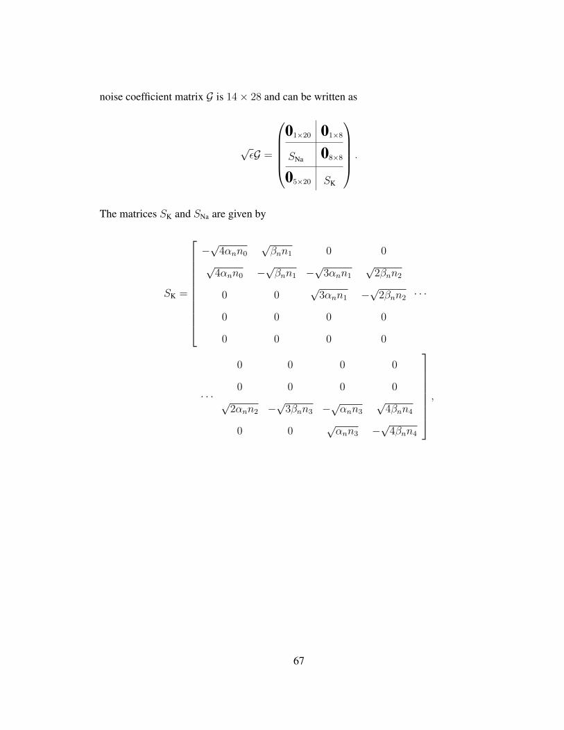
noise coefficient matrix G is 14× 28 and can be written as
√εG =
01×20 01×8
SNa 08×8
05×20 SK
.
The matrices SK and SNa are given by
SK =
−√
4αnn0
√βnn1 0 0
√4αnn0 −
√βnn1 −
√3αnn1
√2βnn2
0 0√
3αnn1 −√
2βnn2
0 0 0 0
0 0 0 0
· · ·
· · ·
0 0 0 0
0 0 0 0√
2αnn2 −√
3βnn3 −√αnn3
√4βnn4
0 0√αnn3 −
√4βnn4
,
67
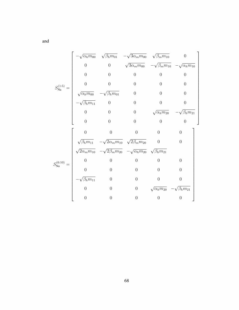
and
S(1:5)Na =
−√αhm00
√βhm01 −
√3αmm00
√βmm10 0
0 0√
3αmm00 −√βmm10 −
√αhm10
0 0 0 0 0
0 0 0 0 0
√αhm00 −
√βhm01 0 0 0
−√βhm11 0 0 0 0
0 0 0√αhm20 −
√βhm21
0 0 0 0 0
S(6:10)Na =
0 0 0 0 0√βhm11 −
√2αmm10
√2βmm20 0 0
√2αmm10 −
√2βmm20 −
√αhm20
√βhm21
0 0 0 0 0
0 0 0 0 0
−√βhm11 0 0 0 0
0 0 0√αhm20 −
√βhm21
0 0 0 0 0
68
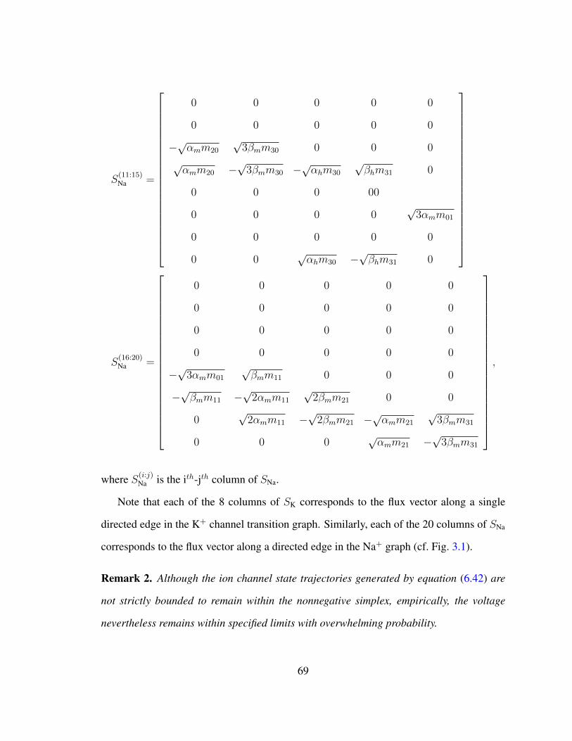
S(11:15)Na =
0 0 0 0 0
0 0 0 0 0
−√αmm20
√3βmm30 0 0 0
√αmm20 −
√3βmm30 −
√αhm30
√βhm31 0
0 0 0 00
0 0 0 0√
3αmm01
0 0 0 0 0
0 0√αhm30 −
√βhm31 0
S(16:20)Na =
0 0 0 0 0
0 0 0 0 0
0 0 0 0 0
0 0 0 0 0
−√
3αmm01
√βmm11 0 0 0
−√βmm11 −
√2αmm11
√2βmm21 0 0
0√
2αmm11 −√
2βmm21 −√αmm21
√3βmm31
0 0 0√αmm21 −
√3βmm31
,
where S(i:j)Na is the ith-jth column of SNa.
Note that each of the 8 columns of SK corresponds to the flux vector along a single
directed edge in the K+ channel transition graph. Similarly, each of the 20 columns of SNa
corresponds to the flux vector along a directed edge in the Na+ graph (cf. Fig. 3.1).
Remark 2. Although the ion channel state trajectories generated by equation (6.42) are
not strictly bounded to remain within the nonnegative simplex, empirically, the voltage
nevertheless remains within specified limits with overwhelming probability.
69
To facilitate comparison of the model (6.16)-(6.41) with prior work [39, 49, 40], we
may rewrite the 14× 28D Langevin description in the equivalent form
CdV
dt= Iapp(t)− gNaM8 (V − VNa)− gKN5 (V − VK)− gleak(V − Vleak), (6.43)
dM
dt= ANaM + SNaξNa, (6.44)
dN
dt= AKM + SKξK, (6.45)
The drift matrices ANa and AK remain the same as in [39], and are the same as in the 14D
deterministic model (5.10)-(5.11). SNa and SK are constructed from direct transitions of the
underlying kinetics in Fig. 3.1, ξNa ∈ R20 and ξK ∈ R8 are vectors of independent Gaussian
white noise processes with zero mean and unit variance.
Fox and Lu’s original approach [39] requires solving a matrix square root equation
SSᵀ = D to obtain a square (8 × 8 for Na+ or 5 × 5 for K+) noise coefficient matrix
consistent with the state-dependent diffusion matrix D. As an advantage, the ion channel
representation (6.43)-(6.45) uses sparse, nonsquare noise coefficient matrices (8 × 20 for
the Na+ channel and 5× 8 for the K+ channel), which exposes the independent sources of
noise for the system.
The new Langevin model in (6.43)-(6.45) does not require detailed balance, which gives
more insights to the underlying kinetics. Review papers such as [49, 61, 93], did systematic
comparison of various stochastic versions of the HH model. In §7 and §8, we quantitaviely
analyze the connection between the new model and other existing models [20, 21, 39, 40,
41, 48, 49, 60, 61, 90, 93]. Problems such as the boundary constrains are beyond the scope
of this dissertation, however, we would like to connect the new model to another type of
approximation to the MC model, namely the stochastic shielding approximation.
70
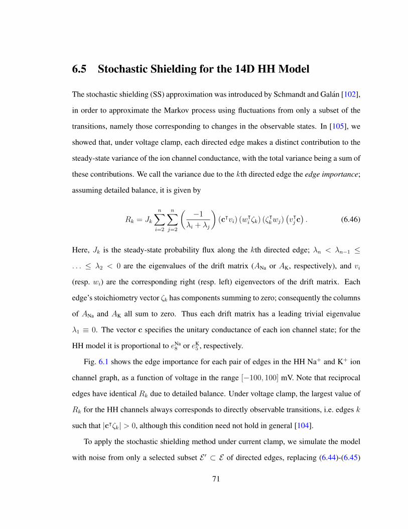
6.5 Stochastic Shielding for the 14D HH Model
The stochastic shielding (SS) approximation was introduced by Schmandt and Galan [102],
in order to approximate the Markov process using fluctuations from only a subset of the
transitions, namely those corresponding to changes in the observable states. In [105], we
showed that, under voltage clamp, each directed edge makes a distinct contribution to the
steady-state variance of the ion channel conductance, with the total variance being a sum of
these contributions. We call the variance due to the kth directed edge the edge importance;
assuming detailed balance, it is given by
Rk = Jk
n∑i=2
n∑j=2
(−1
λi + λj
)(cᵀvi) (wᵀi ζk) (ζᵀkwj)
(vᵀj c). (6.46)
Here, Jk is the steady-state probability flux along the kth directed edge; λn < λn−1 ≤
. . . ≤ λ2 < 0 are the eigenvalues of the drift matrix (ANa or AK, respectively), and vi
(resp. wi) are the corresponding right (resp. left) eigenvectors of the drift matrix. Each
edge’s stoichiometry vector ζk has components summing to zero; consequently the columns
of ANa and AK all sum to zero. Thus each drift matrix has a leading trivial eigenvalue
λ1 ≡ 0. The vector c specifies the unitary conductance of each ion channel state; for the
HH model it is proportional to eNa8 or eK
5 , respectively.
Fig. 6.1 shows the edge importance for each pair of edges in the HH Na+ and K+ ion
channel graph, as a function of voltage in the range [−100, 100] mV. Note that reciprocal
edges have identical Rk due to detailed balance. Under voltage clamp, the largest value of
Rk for the HH channels always corresponds to directly observable transitions, i.e. edges k
such that |cᵀζk| > 0, although this condition need not hold in general [104].
To apply the stochastic shielding method under current clamp, we simulate the model
with noise from only a selected subset E ′ ⊂ E of directed edges, replacing (6.44)-(6.45)
71
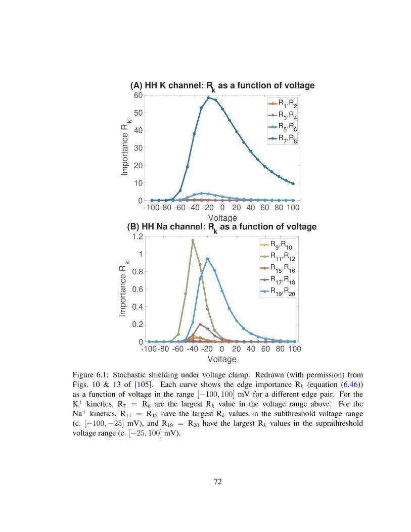
-100-80 -60 -40 -20 0 20 40 60 80 100
Voltage
0
10
20
30
40
50
60
Import
ance R
k
(A) HH K channel: Rk as a function of voltage
R1,R
2
R3,R
4
R5,R
6
R7,R
8
-100-80 -60 -40 -20 0 20 40 60 80 100
Voltage
0
0.2
0.4
0.6
0.8
1
1.2
Import
ance R
k
(B) HH Na channel: Rk as a function of voltage
R9,R
10
R11
,R12
R15
,R16
R17
,R18
R19
,R20
Figure 6.1: Stochastic shielding under voltage clamp. Redrawn (with permission) fromFigs. 10 & 13 of [105]. Each curve shows the edge importance Rk (equation (6.46))as a function of voltage in the range [−100, 100] mV for a different edge pair. For theK+ kinetics, R7 = R8 are the largest Rk value in the voltage range above. For theNa+ kinetics, R11 = R12 have the largest Rk values in the subthreshold voltage range(c. [−100,−25] mV), and R19 = R20 have the largest Rk values in the suprathresholdvoltage range (c. [−25, 100] mV).
72
with
dM
dt= ANaM + S ′NaξNa, (6.47)
dN
dt= AKM + S ′KξK, , (6.48)
where S ′Na (resp. S ′K) is a reduced matrix containing only the noise coefficients from the
most important edges E ′. That is, E ′ contains a subset of edges with the largest edge-
importance values Rk.
In [102], they assumed that the edges with the largest contribution contribution to
current fluctuations under voltage clamp would also make the largest contributions to
variability in voltage and timing under current clamp, and included edges 7 − 8 of the
K+channel (E ′K = 7, 8) and edges 11 − 12 and 19 − 20 of the Na+ channel (E ′Na =
11, 12, 19, 20), yielding an 8× 4 matrix S ′Na and an 5× 2 matrix S ′K. They demonstrated
numerically that restricting stochastic forcing to these edges gave a significantly faster
simulation with little appreciable change in statistical behavior: under voltage clamp, the
mean current remained the same, with a small (but noticeable) decrease in the current
variance; meanwhile similar inter-spike interval (ISI) statistics were observed.
Under current clamp, detailed balance is violated, and it is not clear from mathematical
principles whether the edges with the largest Rk under voltage clamp necessarily make the
largest contribution under other circumstances. In order to evaluate the contribution of the
fluctuations driven by each directed edge on ISI variability, we test the stochastic shielding
method by removing all but one column of Sion at a time. That is, we restrict to a single
noise source and observe the resulting ISI variance empirically. For example, to calculate
the importance of the kth direct edge in the Na+ channel, we suppress the noise from all
73
other edges by setting S ′KξK = 05×1 and
S ′Na =[08×1, · · · , SNa(:, k), · · · ,08×1
]
i.e., only include the kth column of SNa and set other columns to be zeros. The ISI variance
was calculated from an ensemble of 104 voltage traces, each spanning c. 500 ISIs.
Fig. 6.2A plots the logarithm of the ISI variance for each edge in EK. Vertical bars (cyan)
show the ensemble mean of the ISI variance, with a 95% confidence interval superimposed
(magenta). Several observations are in order. First, the ISI variance driven by the noise
in each edge decreases rapidly, the further the edge is from the observable transitions
(edges 7,8), reflecting the underlying “stochastic shielding” phenomenon. Second, the
symmetry of the edge importance for reciprocal edge pairs ((1,2), (3,4), (5,6) and (7,8))
that is observed under voltage clamp is broken under current clamp. The contribution of
individual directed edges to timing variability under current clamp has another important
difference compared with the edge importance (current fluctuations) under voltage clamp.
A similar breaking of symmetry for reciprocal edges is seen for the Na+ channel, again
reflecting the lack of detailed balance during active spiking.
Fig. 6.2B shows the ISI variance when channel noise is included on individual edges
of ENa. Here the difference between voltage and current clamp is striking. Under voltage
clamp, the four most important edges are always those representing “observable transi-
tions”, in the sense that the transition’s stoichiometry vector ζ is not orthogonal to the
conductance vector c. That is, the four most important pairs are always 11-12 and 19-20,
regardless of voltage (Fig. 6.1). Under current clamp, the most important edges are 17,
18, 19 and 20. Although edges 11 and 12 are among the four most important sources of
channel population fluctuations under voltage clamp, they are not even among the top ten
74
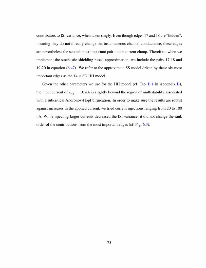
contributors to ISI variance, when taken singly. Even though edges 17 and 18 are “hidden”,
meaning they do not directly change the instantaneous channel conductance, these edges
are nevertheless the second most important pair under current clamp. Therefore, when we
implement the stochastic-shielding based approximation, we include the pairs 17-18 and
19-20 in equation (6.47). We refer to the approximate SS model driven by these six most
important edges as the 14× 6D HH model.
Given the other parameters we use for the HH model (cf. Tab. B.1 in Appendix B),
the input current of Iapp = 10 nA is slightly beyond the region of multistability associated
with a subcritical Andronov-Hopf bifurcation. In order to make sure the results are robust
against increases in the applied current, we tried current injections ranging from 20 to 100
nA. While injecting larger currents decreased the ISI variance, it did not change the rank
order of the contributions from the most important edges (cf. Fig. 6.3).
75
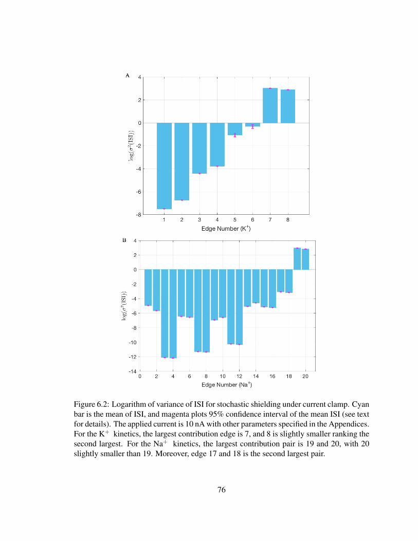
Figure 6.2: Logarithm of variance of ISI for stochastic shielding under current clamp. Cyanbar is the mean of ISI, and magenta plots 95% confidence interval of the mean ISI (see textfor details). The applied current is 10 nA with other parameters specified in the Appendices.For the K+ kinetics, the largest contribution edge is 7, and 8 is slightly smaller ranking thesecond largest. For the Na+ kinetics, the largest contribution pair is 19 and 20, with 20slightly smaller than 19. Moreover, edge 17 and 18 is the second largest pair.
76
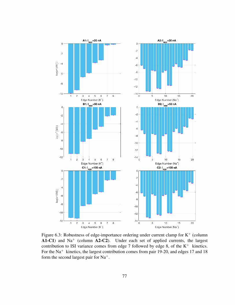
Figure 6.3: Robustness of edge-importance ordering under current clamp for K+ (columnA1-C1) and Na+ (column A2-C2). Under each set of applied currents, the largestcontribution to ISI variance comes from edge 7 followed by edge 8, of the K+ kinetics.For the Na+ kinetics, the largest contribution comes from pair 19-20, and edges 17 and 18form the second largest pair for Na+.
77

Part III
Model Comparison
78
Chapter 7
Pathwise Equivalence for a Class of
Langevin Models
Fox and Lu’s method was widely used since its appearance (see references in [49, 12,
61]), and the “best” approximation for the underlying Markov Chain (MC) model has
been a subject of ongoing discussion for decades. Several studies [12, 81, 111] attested
to discrepancies between Fox’s later approach in [40] and the discrete-state MC model,
raising the question of whether Langevin approximations could ever accurately represent
the underlying fluctuations seen in the “gold standard” MC models. An influential review
paper [49] found that these discrepancies were due to the way in which noise is added to
the stochastic differential equations (3.1)-(3.3). Recent studies including [20, 21, 41, 48,
49, 56, 60, 61, 73, 90, 93] discussed various ways of incorporating channel noise into HH
kinetics based on the original work by Fox and Lu [39, 40], some of which have the same
SDEs but with different boundary conditions. Different boundary conditions (BCs) are not
expected to have much impact on computational efficiency. Indeed, if BCs are neglected,
79
the main difference between channel-based (or conductance-based) models is the diffusion
matrix S in the Langevin euqations (3.2) and (3.3). As the discussion about where and how
to incorporate noise into the HH model framework goes on, [41] recently asked whether
there is a way of relating different models with different S matrices. We give a positive
answer to this question below.
In §7.1 we will demonstrate the equivalence (neglecting the boundary conditions) of a
broad class of previously proposed channel-based Langevin models including: [20, 21, 39,
41, 49, 60, 90, 93] and the 14D Langevin HH model with 28 independent noise sources (one
for each directed edge in the channel state transition graph), i.e. our “14× 28D” Langevin
model.
7.1 When are Two Langevin Equations Equivalent?
Two Langevin models are pathwise equivalent if the sample paths (trajectories) of one
model can be made to be identical to the sample paths of the other, under an appropriate
choice of Gaussian white noise samples for each. To make this notion precise, consider two
channel-based Langevin models of the form dX = f(X) dt + G(X)dW with the same
mean dynamics f ∈ Rd and two different d× n matrices (possibly with different values of
n1 and n2), G1 and G2. Denote
f : Rd → Rd, (7.1)
G1 : Rd → Rd×n1 , (7.2)
G2 : Rd → Rd×n2 . (7.3)
80
Let X(t) = [X1(t), X2(t), . . . , Xd(t)]ᵀ and X∗(t) = [X∗1 (t), X∗2 (t), . . . , X∗d(t)]ᵀ be tra-
jectories produced by the two models and let W(t) = [W1(t),W2(t), . . . ,Wn1(t)]ᵀ and
W∗(t) = [W ∗1 (t),W ∗
2 (t), . . . ,W ∗n2
(t)]ᵀ be vectors of Wiener processes. That is, Wi(t), i =
1, 2, . . . , n1 andW ∗j (t), j = 1, 2, . . . , n2 are independent Wiener processes with 〈Wi(s)Wj(t)〉 =
δijδ(t − s) and 〈W ∗i (s)W ∗
j (t)〉 = δijδ(t − s). Note that n1 and n2 need not be equal. As
defined in [2], the stochastic differential equation (SDE) models
dX = f(t,X(t))dt+G1(t,X(t))dW(t) (7.4)
and
dX∗ = f(t,X∗(t))dt+G2(t,X∗(t))dW∗(t) (7.5)
are pathwise equivalent if systems (7.4) and (7.5) posses the same probability distribution,
and moreover, a sample path solution of one equation is also a sample solution to the
other one. In [2], the authors proved a theorem giving general conditions under which
the trajectories of two SDEs are equivalent. We follow their construction closely below,
adapting it to the case of two different Langevin equations for the Hodgkin-Huxley system
represented in a 14-dimensional state space.
As in §6, channel-based Langevin models for the stochastic dynamics of HH can be
written as
dX = f(X) dt+ S(X)dW(t) (7.6)
where the 14-component random vector X = (V ;M;N) and f(x) =[dVdt
; dMdt
; dNdt
]is the
81
same as the mean-field, eqns. (5.7)-(5.9). Recall that x = [v,m,n]ᵀ. Here we write
S(x) =
01×m 01×n
SNa(m) 08×n
05×m SK(n)
, with
SNa : R8 → R8×m, (7.7)
for the Na+ channel, and
SK : R5 → R5×n, (7.8)
for the K+ channel. Here, m is the number of independent white noise forcing terms
affecting the sodium channel variables, while n is the number of independent noise sources
affecting the potassium gating variables. We write
W(t) = [W1(t),W2(t), . . . ,Wm+n(t)]ᵀ
for a Wiener process incorporating both the sodium and potassium noise forcing. Given
two channel-based models with diffusion matrices
SNa,1 : R8 → R8×m1 , (7.9)
SNa,2 : R8 → R8×m2 , (7.10)
82
for the Na+ channel, and
SK,1 : R5 → R5×n1 , (7.11)
SK,2 : R5 → R5×n2 , (7.12)
for the K+ channel, we construct the diffusion matrix D = SSᵀ. In order for the two
models to generate equivalent sample paths, it suffices that they have the same diffusion
matrix, i.e.
D = S1Sᵀ1 =
01×1 01×8 01×5
08×1 DNa 08×5
05×1 05×8 DK
= S2Sᵀ2 .
The SDEs corresponding to the two channel-based Langevin models are
dX = f(t,X(t))dt+ S1(t,X(t))dW(t), (7.13)
dX∗ = f(t,X∗(t))dt+ S2(t,X∗(t))dW∗(t). (7.14)
The probability density function p(t,x) for random variable X in eqn. (7.13) satisfies
the Fokker-Planck equation
∂p(t,x)
∂t=
1
2
8∑i=1
8∑j=1
∂2
∂xixj
[p(t,x)
m1+n1∑l=1
S(i,l)1 (t,x)S(j,l)
1 (t,x)]
−8∑i=1
∂
∂xi
[fi(t,x)p(t,x)
]=
1
2
8∑i=1
8∑j=1
∂2
∂xixj
[D(i,j)(t,x)p(t,x)
]−
8∑i=1
∂
∂xi
[fi(t,x)p(t,x)
](7.15)
83
where S(i,j)1 (t,x) is the (i, j)th entry of the diffusion matrix S1(t,x). Eqn. (7.15) holds
because
D(i,j)(t,x) =
m1+n1∑l=1
S(i,l)1 (t,x)S(j,l)
1 (t,x).
If z1, z2 ∈ R14 and z1 6 z2, then
P (z1 6 X(t) 6 z2) =
∫ z2,14
z1,14
∫ z2,13
z1,13
· · ·∫ z2,1
z1,1
p(t,x)dx1dx2 · · · dx8.
Note that (7.13) and (7.14) have the same expression (7.15) for the Fokker-Planck equation,
therefore, X and X∗ possess the same probability density function. In other words, the
probability density function of X in eqn. (7.6) is invariant for different choices of the
diffusion matrix S.
7.2 Map Channel-based Langevin Models to Fox and Lu’s
Model
We now explicitly construct a mapping between Fox and Lu’s 14D model [39] and any
channel-based model (given the same boundary conditions). We begin with a channel-
based Langevin description
dX = f(t,X(t))dt+ S(t,X(t))dW(t), (7.16)
and Fox and Lu’s model [39]
dX∗ = f(t,X∗(t))dt+ S0(t,X∗(t))dW∗(t), (7.17)
84
where S is a d by m matrix satisfying SSᵀ = D (note that S is not necessarily a square
matrix), and S0 =√D.
Let T be the total simulation time of the random process in equations (7.16) and (7.17).
For 0 6 t 6 T , denote the singular value decomposition (SVD) of S as
S(t) = P (t)Λ(t)Q(t)
where P (t) is an d × d orthogonal matrix (i.e., P ᵀP = PP ᵀ = Id) and Q(t) is an m ×m
orthogonal matrix, and Λ(t) is a d × m matrix with rank(Λ) = r 6 d positive diagonal
entries and d− r zero diagonal entries.
First, we prove that given a Wiener trajectory, W(t), t ∈ [0, T ] and the solution
to eqn. (7.16), X(t), there exists a Wiener trajectory W∗(t) such that the solution to
eqn. (7.17), X∗, is also a solution to eqn. (7.16). In other words, for a Wiener process
W(t) we can construct a W∗(t), such that X∗(t) = X(t), for 0 ≤ t ≤ T .
Following [2], we construct the vector W∗(t) of d independent Wiener processes as
follows:
W∗(t) =
∫ t
0
P (s)[(Λ(s)Λᵀ(s)
) 12
]+Λ(s)Q(s)dW(s) +
∫ t
0
P (s)dW∗∗(s) (7.18)
for 0 6 t 6 T , where W∗∗(t) is a vector of length d with the first r entries equal to
0 and the next d − r entries independent Wiener processes, and[(Λ(s)Λᵀ(s)
) 12
]+is the
85
pseudoinverse of(Λ(s)Λᵀ(s)
) 12 . Consider that
D(t) = S(t)Sᵀ(t) = P (t)Λ(t)Q(t)[P (t)Λ(t)Q(t)
]ᵀ(7.19)
= P (t)Λ(t)Λᵀ(t)P ᵀ(t) (7.20)
= [S0(t)]2, (7.21)
where S0(t) = P (t)(Λ(t)Λᵀ(t)
) 12P ᵀ(t) is a square root of D, by construction.
The diffusion term on the right side of (7.17) with X∗(t) replaced by X(t) satisfies
S0(t,X(t))dW∗(t)
=S0(t)(P (t)
[(Λ(t)Λᵀ(t)
) 12
]+Λ(t)Q(t)dW(t) + P (t)dW∗∗(t)
)=P (t)
(Λ(t)Λᵀ(t)
) 12P ᵀ(t)P (t)
[(Λ(t)Λᵀ(t)
) 12
]+Λ(t)Q(t)dW(t)
+ P (t)(Λ(t)Λᵀ(t)
) 12P ᵀ(t)P (t)dW∗∗(t)
= P (t)Λ(t)Q(t)dW(t). (7.22)
From the SVD of S=PΛQ, we conclude that
S0(t,X(t))dW∗(t) = S(t,X(t))dW(t). (7.23)
Hence, dX = f(t,X(t))dt + S0(t,X(t))dW∗t , i.e., X(t) is a sample path solution of
equation (7.17).
Similarly, given a Wiener trajectory W∗(t) and the solution to eqn. (7.17) X∗(t), we
can construct a vector W(t) of m independent Wiener processes as
W(t) =
∫ t
0
Qᵀ(s)Λ+(s)[Λ(s)Λᵀ(s)
]1/2P ᵀ(s)dW∗(s) +
∫ t
0
Qᵀ(s)dW∗∗∗(s) (7.24)
86
for 0 6 t 6 T , where W∗∗∗(t) is a vector of length m with the first r entries equal to 0
and the next m− r entries independent Wiener processes, and Λ+(s) is the pseudoinverse
of Λ(s). Then, by an argument parallel to (7.22), we conclude that
S(t,X∗(t))dW (t) = S0(t,X∗(t))dW∗(t). (7.25)
Hence, dX∗ = f(t,X∗(t))dt + S(t,X∗(t))dW(t), that is, X∗(t) is also a solution to
(7.16). Therefore we can conclude that the channel-based Langevin model in eqn. (7.16) is
pathwise equivalent to the Fox and Lu’s model.
To illustrate pathwise equivalence, Fig. 7.1 plots trajectories of the 14× 28D stochastic
HH model and Fox and Lu’s model, using noise traces dictated by the preceding construc-
tion. In panel A, we generated a sample path for eqn. (7.16) and plot three variables in X:
the voltage V , Na+ channel open probability M31 and K+ channel open probability N4.
The corresponding trajectory, X∗, for Fox and Lu’s model was generated from eqn. (7.17)
and the corresponding Wiener trajectory was calculated using eqn. (7.18). To see that
these trajectories are pathwise equivalent, in the top three subplots in panel A (resp. B)
we superposed the voltage V ∗, Na+ channel open probability M∗31 and K+ channel open
probability N∗4 in X∗ against those in X. The bottom three subplots in panel A (resp. B)
plot the point-wise differences of each variable. Eqns. (7.16) and (7.17) are numerically
solved in Matlab using the Euler-Maruyama method with a time step dt = 0.001ms. The
slight differences observed arise in part due to numerical errors in calculating the singular
value decomposition of S (in eqn. (7.16)); another source of error is the finite accuracy
of the Euler-Maruyama method.1 As shown in Fig. 7.1, most differences occur near the
spiking region, where the system is numerically very stiff and the numerical accuracy of
1The forward Euler method is first order accurate for ordinary differential equations, but the forwardEuler-Maruyama method is only O(
√dt) accurate for stochastic differential equations [68].
87
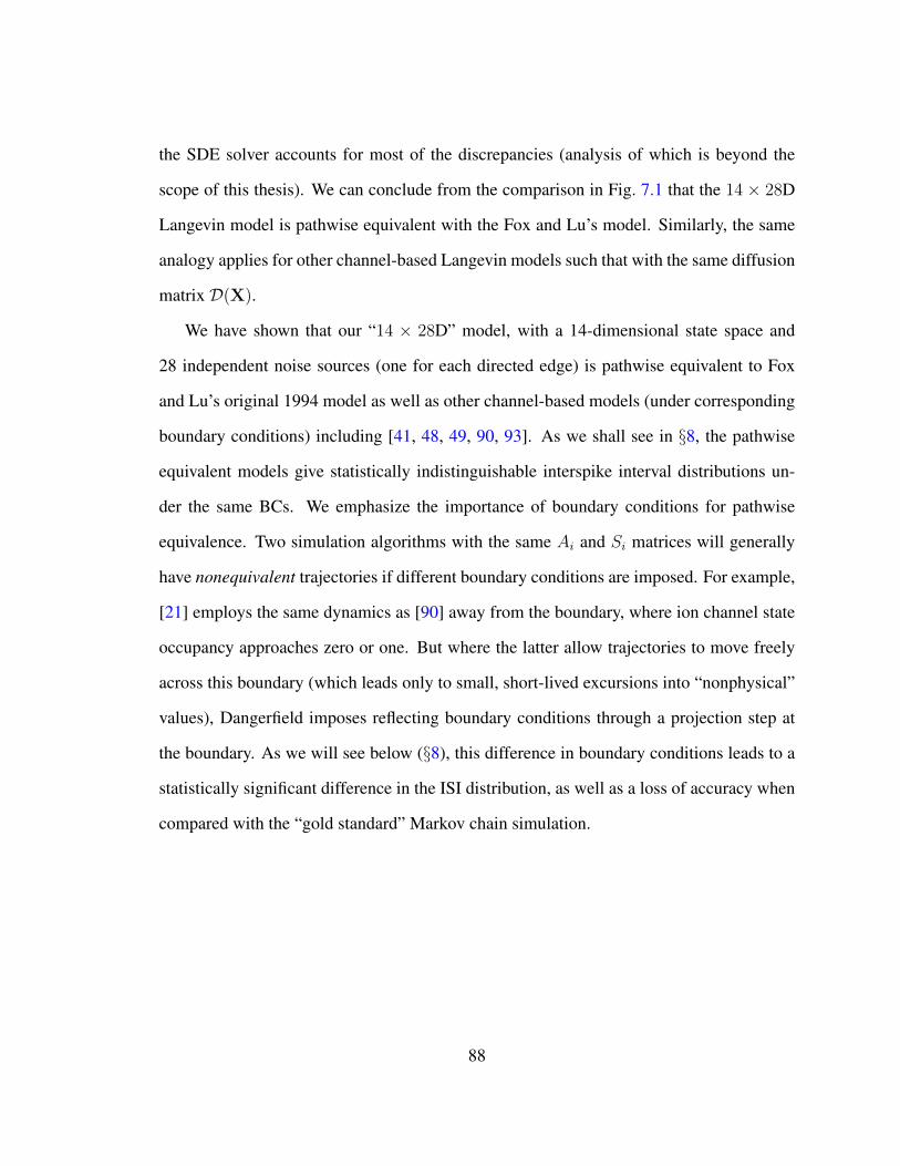
the SDE solver accounts for most of the discrepancies (analysis of which is beyond the
scope of this thesis). We can conclude from the comparison in Fig. 7.1 that the 14 × 28D
Langevin model is pathwise equivalent with the Fox and Lu’s model. Similarly, the same
analogy applies for other channel-based Langevin models such that with the same diffusion
matrix D(X).
We have shown that our “14 × 28D” model, with a 14-dimensional state space and
28 independent noise sources (one for each directed edge) is pathwise equivalent to Fox
and Lu’s original 1994 model as well as other channel-based models (under corresponding
boundary conditions) including [41, 48, 49, 90, 93]. As we shall see in §8, the pathwise
equivalent models give statistically indistinguishable interspike interval distributions un-
der the same BCs. We emphasize the importance of boundary conditions for pathwise
equivalence. Two simulation algorithms with the same Ai and Si matrices will generally
have nonequivalent trajectories if different boundary conditions are imposed. For example,
[21] employs the same dynamics as [90] away from the boundary, where ion channel state
occupancy approaches zero or one. But where the latter allow trajectories to move freely
across this boundary (which leads only to small, short-lived excursions into “nonphysical”
values), Dangerfield imposes reflecting boundary conditions through a projection step at
the boundary. As we will see below (§8), this difference in boundary conditions leads to a
statistically significant difference in the ISI distribution, as well as a loss of accuracy when
compared with the “gold standard” Markov chain simulation.
88
Figure 7.1: Pathwise equivalency of 14D HH model and Fox and Lu’s model. A: Givena sample path of the 14 × 28D Langevin model in eqn. (7.16), we construct the noise byeqn. (7.18) and generate the sample trajectory of Fox and Lu’s model using eqn. (7.17).B: Given a sample path of Fox and Lu’s model in eqn. (7.17), we construct the noise byeqn. (7.24) and generate the sample trajectory of the 14 × 28D Langevin model usingeqn. (7.16). We obtain excellent agreement in both directions. See text for details.
89
Chapter 8
Model Comparison
In §6, we studied the contribution of every directed edge to the ISI variability and proposed
how stochastic shielding could be applied under current clamp. Moreover, in §7, we proved
that a family of Langevin models are pathwise equivalent.
Here we compare the accuracy and computational efficiency of several models, includ-
ing the “subunit model” [40, 49], Langevin models with different S matrices or boudary
conditions [21, 39, 49, 90, 93], the 14D HH model (proposed in §6.3), the 14D stochastic
shielding model with six independent noise sources (proposed in §6.5), and the “gold
standard” Markov Chain model (discussed in §6.2). Where other studies have compared
moment statistics such as the mean firing frequency (under current clamp) and stationary
channel open probababilies (under voltage clamp), we base our comparison on the entire
interspike interval (ISI) distributions, under current clamp with a common fixed driving
current. We use two different comparisons of ISI distributions, the first based on the L1
norm of the difference between two distributions (the Wasserstein distance, [124]), in §8.1
and the second based on the L∞ norm (the Kolmogorov-Smirnov test, [69, 117]), in §8.2.
90
We find similar results using both measures: as expected, the models that produce pathwise
equivalent trajectories (Fox & Lu ’94, Orio & Soudry, and our 14 × 28D model) have
indistinguishable ISI statistics, while the non-equivalent models (Fox ’97, Dangerfield,
Goldwyn & Shea-Brown, our 14 × 6D stochastic-shielding model) have significantly dif-
ferent ISI distributions. Of these, the 14× 6D SS model is the closest to the models in the
14× 28D class, and as fast as any other model considered.
8.1 L1 Norm Difference of ISIs
We first evaluate the accuracy of different stochastic simulation algorithms by comparing
their ISI distributions under current clamp to that produced by a reference algorithm,
namely the discrete-state Markov Chain (MC) algorithm.
Let X1, X2, . . . , Xn be n independent samples of ISIs with a true cumulative distri-
bution function F . Let Fn(·) denote the corresponding empirical cumulative distribution
function (ECDF) defined by
Fn(x) =1
n
n∑i=1
1Xi≤x, x ∈ R, (8.1)
where we write 1A to denote the indicator function for the set A. Let Q and QM be the
quantile functions of F and FM , respectively. The L1-Wasserstein distance between two
CDF’s FM and F can be written as [114] (page 64)
ρ1(F, FM) =
∫ ∞0
∣∣F (x)− FM(x)∣∣ dx =
∫ 1
0
∣∣Q(x)−QM(x)∣∣ dx. (8.2)
Note that ρ1 has the same units as “dx”. Thus the L1 distances reported in Tab. 8.1 have
units of milliseconds.
91
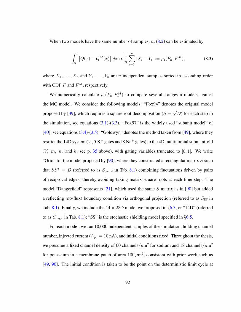
When two models have the same number of samples, n, (8.2) can be estimated by
∫ 1
0
∣∣Q(x)−QM(x)∣∣ dx ≈ 1
n
n∑i=1
|Xi − Yi| := ρ1(Fn, FMn ), (8.3)
where X1, · · · , Xn and Y1, · · · , Yn are n independent samples sorted in ascending order
with CDF F and FM , respectively.
We numerically calculate ρ1(Fn, FMn ) to compare several Langevin models against
the MC model. We consider the following models: “Fox94” denotes the original model
proposed by [39], which requires a square root decomposition (S =√D) for each step in
the simulation, see equations (3.1)-(3.3). “Fox97” is the widely used “subunit model” of
[40], see equations (3.4)-(3.5). “Goldwyn” denotes the method taken from [49], where they
restrict the 14D system (V , 5 K+ gates and 8 Na+ gates) to the 4D multinomial submanifold
(V, m, n, and h, see p. 35 above), with gating variables truncated to [0, 1]. We write
“Orio” for the model proposed by [90], where they constructed a rectangular matrix S such
that SSᵀ = D (referred to as Spaired in Tab. 8.1) combining fluctuations driven by pairs
of reciprocal edges, thereby avoiding taking matrix square roots at each time step. The
model “Dangerfield” represents [21], which used the same S matrix as in [90] but added
a reflecting (no-flux) boundary condition via orthogonal projection (referred to as SEF in
Tab. 8.1). Finally, we include the 14× 28D model we proposed in §6.3, or “14D” (referred
to as Ssingle in Tab. 8.1); “SS” is the stochastic shielding model specified in §6.5.
For each model, we ran 10,000 independent samples of the simulation, holding channel
number, injected current (Iapp = 10 nA), and initial conditions fixed. Throughout the thesis,
we presume a fixed channel density of 60 channels/µm2 for sodium and 18 channels/µm2
for potassium in a membrane patch of area 100µm2, consistent with prior work such as
[49, 90]. The initial condition is taken to be the point on the deterministic limit cycle at
92
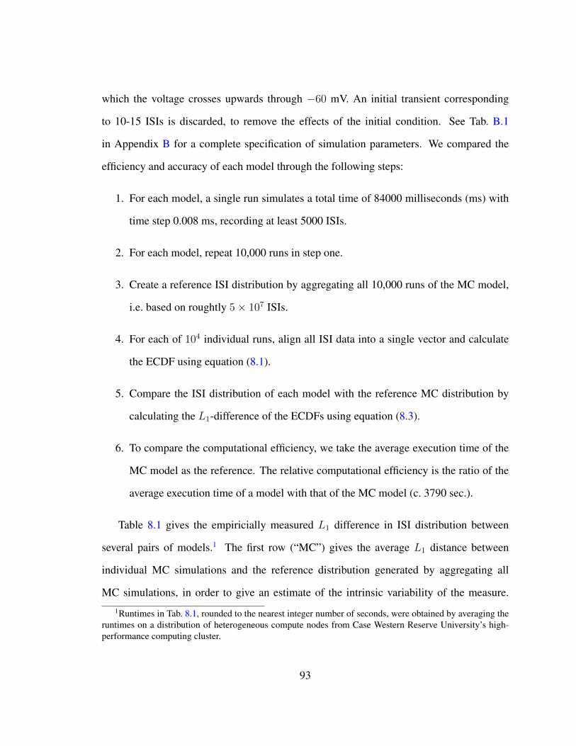
which the voltage crosses upwards through −60 mV. An initial transient corresponding
to 10-15 ISIs is discarded, to remove the effects of the initial condition. See Tab. B.1
in Appendix B for a complete specification of simulation parameters. We compared the
efficiency and accuracy of each model through the following steps:
1. For each model, a single run simulates a total time of 84000 milliseconds (ms) with
time step 0.008 ms, recording at least 5000 ISIs.
2. For each model, repeat 10,000 runs in step one.
3. Create a reference ISI distribution by aggregating all 10,000 runs of the MC model,
i.e. based on roughtly 5× 10⁷ ISIs.
4. For each of 104 individual runs, align all ISI data into a single vector and calculate
the ECDF using equation (8.1).
5. Compare the ISI distribution of each model with the reference MC distribution by
calculating the L1-difference of the ECDFs using equation (8.3).
6. To compare the computational efficiency, we take the average execution time of the
MC model as the reference. The relative computational efficiency is the ratio of the
average execution time of a model with that of the MC model (c. 3790 sec.).
Table 8.1 gives the empiricially measured L1 difference in ISI distribution between
several pairs of models.1 The first row (“MC”) gives the average L1 distance between
individual MC simulations and the reference distribution generated by aggregating all
MC simulations, in order to give an estimate of the intrinsic variability of the measure.
1Runtimes in Tab. 8.1, rounded to the nearest integer number of seconds, were obtained by averaging theruntimes on a distribution of heterogeneous compute nodes from Case Western Reserve University’s high-performance computing cluster.
93
Model Variables S Matrix Noise Dim. L1 Norm (msec.) RuntimeV+M+N Na+K (Wasserstein Dist.) (sec.)
MC 1+8+5 n/a 20+8 2.27 e-4± 7.15 e-5 3790Fox94 1+7+4 S =
√D 7+4 4.74 e-2± 1.93 e-4 2436
Fox97 1+2+1 n/a 3 8.01 e-1± 9.48 e-4 67Dangerfield 1+8+5 SEF 10+4 2.18 e-1± 2.14 e-4 655Goldwyn 1+8+5 S =
√D 8+5 1.83 e-1± 1.93 e-4 2363
Orio 1+8+5 Spaired 10+4 4.52 e-2± 2.08 e-4 57714× 28D 1+8+5 Ssingle 20+8 4.93 e-2± 1.94 e-4 605SS 1+8+5 Sss 4+2 7.62 e-2± 7.57 e-5 73
Table 8.1: Summary of the L1-Wasserstein distances of ISI distributions for Langevin typeHodgkin-Huxley models compared to the MC model. Model (see text for details): MC:Markov-chain. Fox1994: model from [39]. Fox97: [40]. Goldwyn: [49]. Dangerfield:[21, 20]. 14 × 28D: model proposed in §6.3. SS: stochastic-shielding model (§6.5).Variables: number of degrees of freedom in Langevin equation representing voltage,sodium gates, and potassium gates, respectively. S Matrix: Form of the noise coefficientmatrix in equations (3.1)-(3.3). Noise Dimensions: number of independent Gaussian white-noise sources represented for sodium and potassium, respectively. L1 Norm: Empiricallyestimated L1-Wasserstein distance between the model’s ISI distribution and the MCmodel’s ISI distribution. For MC-vs-MC, independent trials were compared. a ± b:mean±standard deviation. Runtime (in sec.): see text for details. n/a: not applicable.
94
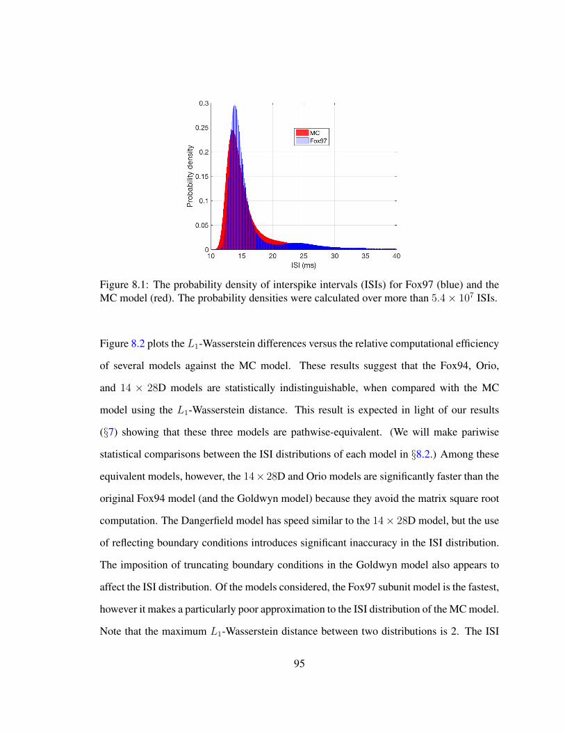
Figure 8.1: The probability density of interspike intervals (ISIs) for Fox97 (blue) and theMC model (red). The probability densities were calculated over more than 5.4× 10⁷ ISIs.
Figure 8.2 plots the L1-Wasserstein differences versus the relative computational efficiency
of several models against the MC model. These results suggest that the Fox94, Orio,
and 14 × 28D models are statistically indistinguishable, when compared with the MC
model using the L1-Wasserstein distance. This result is expected in light of our results
(§7) showing that these three models are pathwise-equivalent. (We will make pariwise
statistical comparisons between the ISI distributions of each model in §8.2.) Among these
equivalent models, however, the 14× 28D and Orio models are significantly faster than the
original Fox94 model (and the Goldwyn model) because they avoid the matrix square root
computation. The Dangerfield model has speed similar to the 14× 28D model, but the use
of reflecting boundary conditions introduces significant inaccuracy in the ISI distribution.
The imposition of truncating boundary conditions in the Goldwyn model also appears to
affect the ISI distribution. Of the models considered, the Fox97 subunit model is the fastest,
however it makes a particularly poor approximation to the ISI distribution of the MC model.
Note that the maximum L1-Wasserstein distance between two distributions is 2. The ISI
95
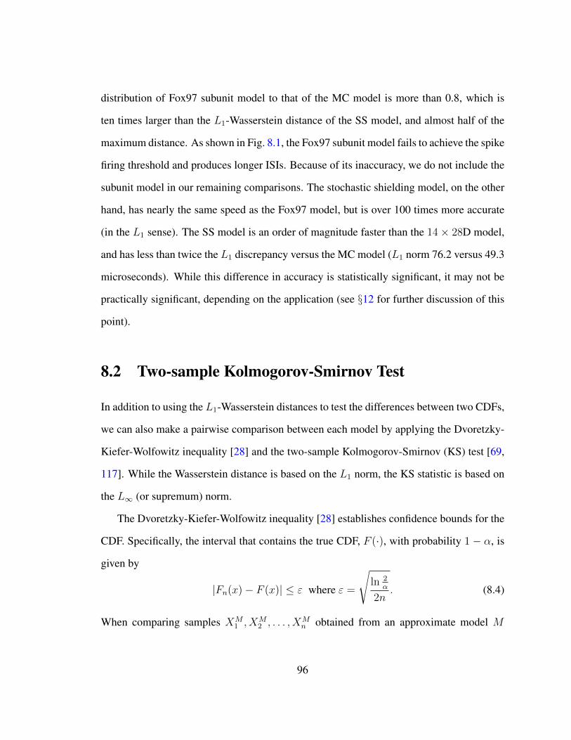
distribution of Fox97 subunit model to that of the MC model is more than 0.8, which is
ten times larger than the L1-Wasserstein distance of the SS model, and almost half of the
maximum distance. As shown in Fig. 8.1, the Fox97 subunit model fails to achieve the spike
firing threshold and produces longer ISIs. Because of its inaccuracy, we do not include the
subunit model in our remaining comparisons. The stochastic shielding model, on the other
hand, has nearly the same speed as the Fox97 model, but is over 100 times more accurate
(in the L1 sense). The SS model is an order of magnitude faster than the 14× 28D model,
and has less than twice the L1 discrepancy versus the MC model (L1 norm 76.2 versus 49.3
microseconds). While this difference in accuracy is statistically significant, it may not be
practically significant, depending on the application (see §12 for further discussion of this
point).
8.2 Two-sample Kolmogorov-Smirnov Test
In addition to using the L1-Wasserstein distances to test the differences between two CDFs,
we can also make a pairwise comparison between each model by applying the Dvoretzky-
Kiefer-Wolfowitz inequality [28] and the two-sample Kolmogorov-Smirnov (KS) test [69,
117]. While the Wasserstein distance is based on the L1 norm, the KS statistic is based on
the L∞ (or supremum) norm.
The Dvoretzky-Kiefer-Wolfowitz inequality [28] establishes confidence bounds for the
CDF. Specifically, the interval that contains the true CDF, F (·), with probability 1 − α, is
given by
|Fn(x)− F (x)| ≤ ε where ε =
√ln 2
α
2n. (8.4)
When comparing samples XM1 , X
M2 , . . . , X
Mn obtained from an approximate model M
96
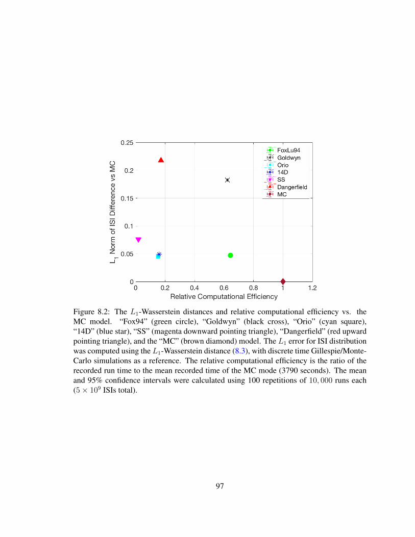
Figure 8.2: The L1-Wasserstein distances and relative computational efficiency vs. theMC model. “Fox94” (green circle), “Goldwyn” (black cross), “Orio” (cyan square),“14D” (blue star), “SS” (magenta downward pointing triangle), “Dangerfield” (red upwardpointing triangle), and the “MC” (brown diamond) model. The L1 error for ISI distributionwas computed using the L1-Wasserstein distance (8.3), with discrete time Gillespie/Monte-Carlo simulations as a reference. The relative computational efficiency is the ratio of therecorded run time to the mean recorded time of the MC mode (3790 seconds). The meanand 95% confidence intervals were calculated using 100 repetitions of 10, 000 runs each(5× 10⁹ ISIs total).
97
against the gold standard, in §8.1 we computed the L1 difference of the empirical density
functions, as an approximation for the L1 difference of the true distributions. Instead, we
work here with the L∞ norm,
ρ∞(Fn, FMn ) = lim
p→∞
(∫ ∞0
∣∣FMn (x)− Fn(x)
∣∣p dx)1/p
= sup0≤x<∞
(∣∣FMn (x)− Fn(x)
∣∣) .(8.5)
For each x ≥ 0, equation (8.4) bounds the discrepancy between the true and empirical
distribution differences as follows. By the triangle inequality, and independence of the Xi
from the XMi , the inequality
|FM − F | = |FM − FMn + Fn − F + FM
n − Fn|
≤ |FM − FMn |+ |Fn − F |+ |FM
n − Fn|
≤ 2ε+ |FMn − Fn|, (8.6)
holds with probability (1− α)2. Similarly,
|FMn − Fn| = |FM
n − FMn + F − Fn + FM − F |
≤ |FM − FMn |+ |Fn − F |+ |FM − F |
≤ 2ε+ |FM − F | (8.7)
also holds with probability (1 − α)2. Together, (8.6)-(8.7) indicate that the discrepancy
between the difference of empirical distributions and the difference of true distributions is
bounded as ∣∣∣|FM − F | − |FMn − Fn|
∣∣∣ ≤ 2ε (8.8)
with probability (1− α)2, for ε =
√ln 2α
2n.
98
We will use the pointwise difference of the ECDF’s for a large sample as an estimate for
the pointwise difference between two true CDFs. The two-sample Kolmogorov-Smirnov
(KS) test [69, 117] offers a statistics to test whether two samples are from the same distri-
bution. The two-sample KS statistic is
Dn,m = supx|F1,n(x)− F2,m(x)|, (8.9)
where F1,n and F2,m are two ECDFs for two samples defined in (8.1), and the sup is the
supremum function. The reference statistic, Rn,m(α), depending on the significance level
α, is defined as
Rn,m(α) =
√− log(α/2)
2
√n+m
nm, (8.10)
where n and m are the sample sizes. The null hypothesis that “the two samples come from
the same distribution” is rejected at the significance level α if
Dn,m > Rn,m(α). (8.11)
Figure 8.3 plots the logarithm of ratio of the two-sample KS statistics, Dn,mRn,m(0.01)
, for
“Fox94” [39], “Goldwyn” [49],“Dangerfiled” [21], “Orio” [90], “14D” (the 14×28D model
we proposed in §6.3). Data of “self-comparison” (e.g. Fox94 vs. Fox 94) was obtained by
comparing two ISI ECDF’s from independent simulations. As shown in Fig. 8.3, models
that we previously proved were pathwise equivalent in §7, namely the “Fox94”, “Orio”
and the “14D” model, are not distinguishable at any confidence level justified by our data.
Note that those three models use the same boundary conditions (free boundary condition as
in [90]) and the ratio Dn,m/Rn,m(α) of pairwise comparison is on the same magnitude of
that for the self-comparisons. However, as pointed out above, these statistically equivalent
99
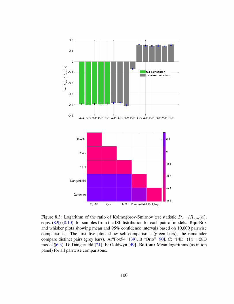
Figure 8.3: Logarithm of the ratio of Kolmogorov-Smirnov test statistic Dn,m/Rn,m(α),eqns. (8.9)-(8.10), for samples from the ISI distribution for each pair of models. Top: Boxand whisker plots showing mean and 95% confidence intervals based on 10,000 pairwisecomparisons. The first five plots show self-comparisons (green bars); the remaindercompare distinct pairs (grey bars). A:“Fox94” [39], B:“Orio” [90], C: “14D” (14 × 28Dmodel §6.3), D: Dangerfield [21], E: Goldwyn [49]. Bottom: Mean logarithms (as in toppanel) for all pairwise comparisons.
100
simulation algorithms have different computational efficiencies (Fig. 8.2). Among these
methods, Orio and Soundry’s algorithm (14 dimensional state space with 14 undirected
edges as noise sources) and our method (14 dimensional state space with 28 directed edges
as noise sources) have similar efficiencies, with Orio’s method being about 5% faster than
ours method. Our 14 × 28D method provides the additional advantage that it facilitates
further acceleration under the stochastic shielding approximation (see §12).
In contrast to the statistically equivalent Orio, 14×28D and Fox ’94 models, algorithms
using different boundary conditions are not pathwise equivalent, which is again verified in
Fig. 8.3. Algorithms with subunit approximation and truncated boundary condition (i.e.,
“Goldwyn”) and the reflecting boundary condition (i.e. “Dangerfield”) are significantly
different in accuracy (and in particular, they are less accurate) than models in the 14× 28D
class.
101
Part IV
Applications of the 14× 28D Langevin Model
102
Chapter 9
Definitions, Notations and Terminology
In this chapter, we will present definitions, notations and terminology that are necessary
for the main applications of the 14 × 28D HH model. We adopt the standard convention
that uppercase symbols (e.g. V,M,N) represent random variables, while corresponding
lowercase symbols (e.g. v,m,n) represent possible realizations of the random variables.
Thus P(V ≤ v) is the probability that the random voltage V does not exceed the value v.
We set vectors in bold font and scalars in standard font.
9.1 The HH Domain
Recall the 14× 28D Langevin model
CdV
dt= Iapp(t)− gNaM8 (V − VNa)− gKN5 (V − VK)− gleak(V − Vleak), (9.1)
dM
dt= ANaM + SNaξNa, (9.2)
dN
dt= AKM + SKξK. (9.3)
103
The drift matrices ANa and AK, SNa and SK are given in §6.3, ξNa ∈ R20 and ξK ∈ R8 are
vectors of independent Gaussian white noise processes with zero mean and unit variance.
Reversal potentials Vion for physiological ions are typically confined to the range ±150mV.
For the 4-D and the 14-D HH models, the reversal potentials for K+ and Na+ are -77mV and
+50mV respectively [32]. In Lemma 3, we establish that the voltage for conductance-based
model in eqn. (9.1)-(9.3) is bounded. Therefore we can find a voltage range [vmin, vmax]
that is forward invariant with probability 1, meaning that the probability of any sample
path leaving the range vmin ≤ V (t) ≤ vmax is zero. At the same time, the channel state
distribution for any channel with k states is restricted to a (k − 1)-dimensional simplex
∆k−1 ⊂ Rk, given by y1 + . . . + yk = 1, yi ≥ 0. Therefore, the phase space of any
conductance-based model of the form eqn. (9.1)-(9.3) may be restricted to a compact
domain in finite dimensions.
Definition 1. We define the HH domain D to be
D ∆= [vmin, vmax]×∆7 ×∆4 (9.4)
where ∆7 is the simplex occupied by the Na+channel states, and ∆4 is occupied by the
K+channel states.
We thus represent the “14-D” HH model in a reduced phase space of dimension 1+7+4=12.
Lemma 3. For a conductance-based model of the form in eqn. (9.1)-(9.3), and for any
bounded applied current I− ≤ Iapp ≤ I+, there exist upper and lower bounds vmax and
vmin such that trajectories with initial voltage condition v ∈ [vmin, vmax] remain within this
interval for all times t > 0, with probability 1, regardless of the initial channel state.
Proof. Let V1 = minionVion ∧ Vleak, and V2 = max
ionVion ∨ Vleak, where ion ∈ Na+,K+.
Note that for both the Na+ and K+ channel, 0 ≤ M8 ≤ 1, 0 ≤ N5 ≤ 1, with probability
104
1. Moreover, gi > 0, gleak > 0, therefore when V ≤ V1
dV
dt=
1
CIapp(t)− gNaM8 (V − VNa)− gKN5 (V − VK)− gleak(V − Vleak) (9.5)
≥ 1
CIapp(t)− gNaM8 (V − V1)− gKN5 (V − V1)− gleak(V − V1) (9.6)
≥ 1
CIapp(t)− 0×M8 (V − V1)− 0×N5 (V − V1)− gleak(V − V1) (9.7)
=1
CIapp(t)− gleak(V − V1) . (9.8)
Inequality (9.6) holds with probability 1 because V1 = mini∈IVi ∧ Vleak, and inequality
(9.7) follows because V − V1 ≤ 0, gi > 0 and M8 ≥ 0, N5 ≥ 0 with probability 1. Let
Vmin := min
I−gleak
+ V1, V1
. When V < Vmin, dV
dt> 0 with probability 1. Therefore, V
will not decrease beyond Vmin with probability 1.
Similarly, when V ≥ V2
dV
dt=
1
CIapp(t)− gNaM8 (V − VNa)− gKN5 (V − VK)− gleak(V − Vleak) (9.9)
≤ 1
CIapp(t)− gNaM8 (V − V2)− gKN5 (V − V2)− gleak(V − V2) (9.10)
≤ 1
CIapp(t)− 0×M8 (V − V2)− 0×N5 (V − V2)− gleak(V − V2) (9.11)
=1
CIapp(t)− gleak(V − V2) . (9.12)
Inequality (9.10) and inequality (9.11) holds with probability 1 because V2 = maxi∈IVi∨
Vleak, V − V2 ≥ 0, gi > 0 and M8 ≥ 0, N5 ≥ 0 with probability 1. Let Vmax =
maxIapp
gleak+ V2, V2
. When V > Vmax,
dVdt
< 0 with probability 1. Therefore, V will
not go beyond Vmax with probability 1.
We conclude that if V takes an initial condition in the interval [Vmin, Vmax], then V (t)
remains within this interval for all t ≥ 0 with probability 1.
105
Throughout this thesis, we use the parameters of the standard Hodgkin-Huxley model,
with constant applied current Iapp = 10 nano Amperes (see Tab. B.1). For these parameters,
Vmin = −77 mV and Vmax ≈ +83.33 mV.
Remark 3. Lemma 3 implies that the per capita transition rates along a finite collection of
edges, αk(v)Kk=1 are bounded above by a constant αmax, as v ranges over vmin ≤ v ≤ vmax.
This fact will help establish Theorem 4.
9.2 Interspike Intervals and First Passage Times
Figure 9.1 shows a voltage trajectory generated by the 14-D stochastic HH model, under
current clamp, with injected current in the range supporting steady firing. The regular
periodicity of the deterministic model vanishes in this case. Nevertheless, the voltage
generates spikes, which allows us to introduce a well defined series of spike times and inter-
spike intervals (ISIs). For example, we may select a reference voltage such as vth = −20
mV, with the property that within a neighborhood of this voltage, trajectories have strictly
positive or strictly negative derivatives (dV/dt) with high probability.
In [100], they suggested that the stochastic (Langevin) 4-D HH model has a unique
invariant stationary joint density for the voltage and gating variables, as well as producing
a stationary point process of spike times. The ensemble of trajectories may be visualized
by aligning the voltage spikes (Figure 9.1b), and illustrates that each trace is either rapidly
increasing or else rapidly decreasing as it passes vth = −20 mV.
In order to give a precise definition of the interspike interval, on which we can base a
first-passage time analysis, we will consider two types of Poincare section of the fourteen-
106
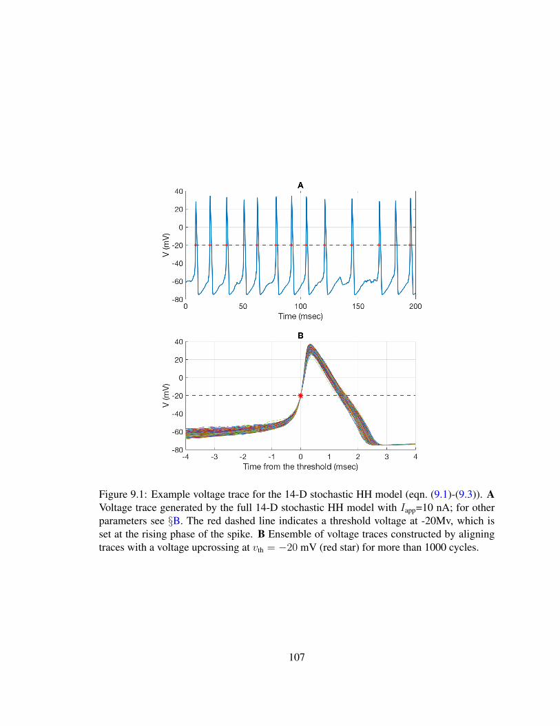
Figure 9.1: Example voltage trace for the 14-D stochastic HH model (eqn. (9.1)-(9.3)). AVoltage trace generated by the full 14-D stochastic HH model with Iapp=10 nA; for otherparameters see §B. The red dashed line indicates a threshold voltage at -20Mv, which isset at the rising phase of the spike. B Ensemble of voltage traces constructed by aligningtraces with a voltage upcrossing at vth = −20 mV (red star) for more than 1000 cycles.
107
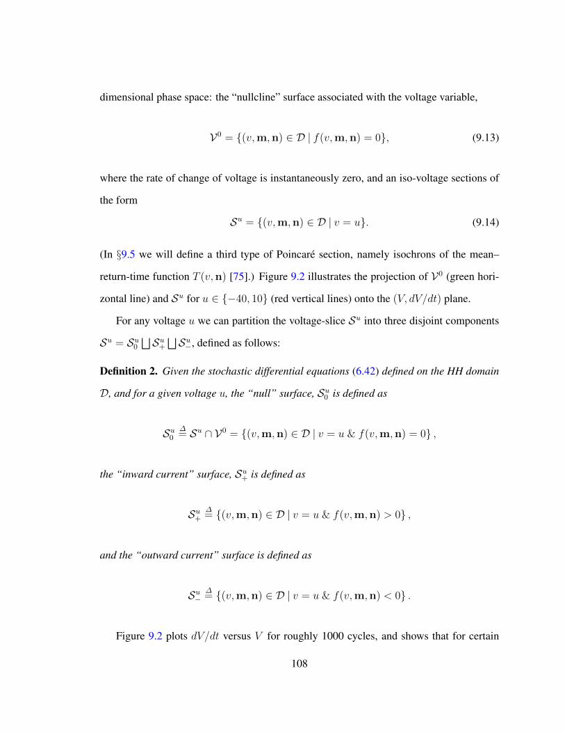
dimensional phase space: the “nullcline” surface associated with the voltage variable,
V0 = (v,m,n) ∈ D | f(v,m,n) = 0, (9.13)
where the rate of change of voltage is instantaneously zero, and an iso-voltage sections of
the form
Su = (v,m,n) ∈ D | v = u. (9.14)
(In §9.5 we will define a third type of Poincare section, namely isochrons of the mean–
return-time function T (v,n) [75].) Figure 9.2 illustrates the projection of V0 (green hori-
zontal line) and Su for u ∈ −40, 10 (red vertical lines) onto the (V, dV/dt) plane.
For any voltage u we can partition the voltage-slice Su into three disjoint components
Su = Su0⊔Su+⊔Su−, defined as follows:
Definition 2. Given the stochastic differential equations (6.42) defined on the HH domain
D, and for a given voltage u, the “null” surface, Su0 is defined as
Su0∆= Su ∩ V0 = (v,m,n) ∈ D | v = u & f(v,m,n) = 0 ,
the “inward current” surface, Su+ is defined as
Su+∆= (v,m,n) ∈ D | v = u & f(v,m,n) > 0 ,
and the “outward current” surface is defined as
Su−∆= (v,m,n) ∈ D | v = u & f(v,m,n) < 0 .
Figure 9.2 plots dV/dt versus V for roughly 1000 cycles, and shows that for certain
108
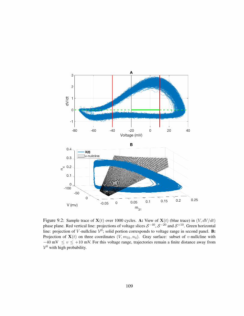
Figure 9.2: Sample trace of X(t) over 1000 cycles. A: View of X(t) (blue trace) in (V, dV/dt)phase plane. Red vertical line: projections of voltage slices S−40, S−20 and S+10. Green horizontalline: projection of V -nullcline V0; solid portion corresponds to voltage range in second panel. B:Projection of X(t) on three coordinates (V,m31, n4). Gray surface: subset of v-nullcline with−40 mV ≤ v ≤ +10 mV. For this voltage range, trajectories remain a finite distance away fromV0 with high probability.
109
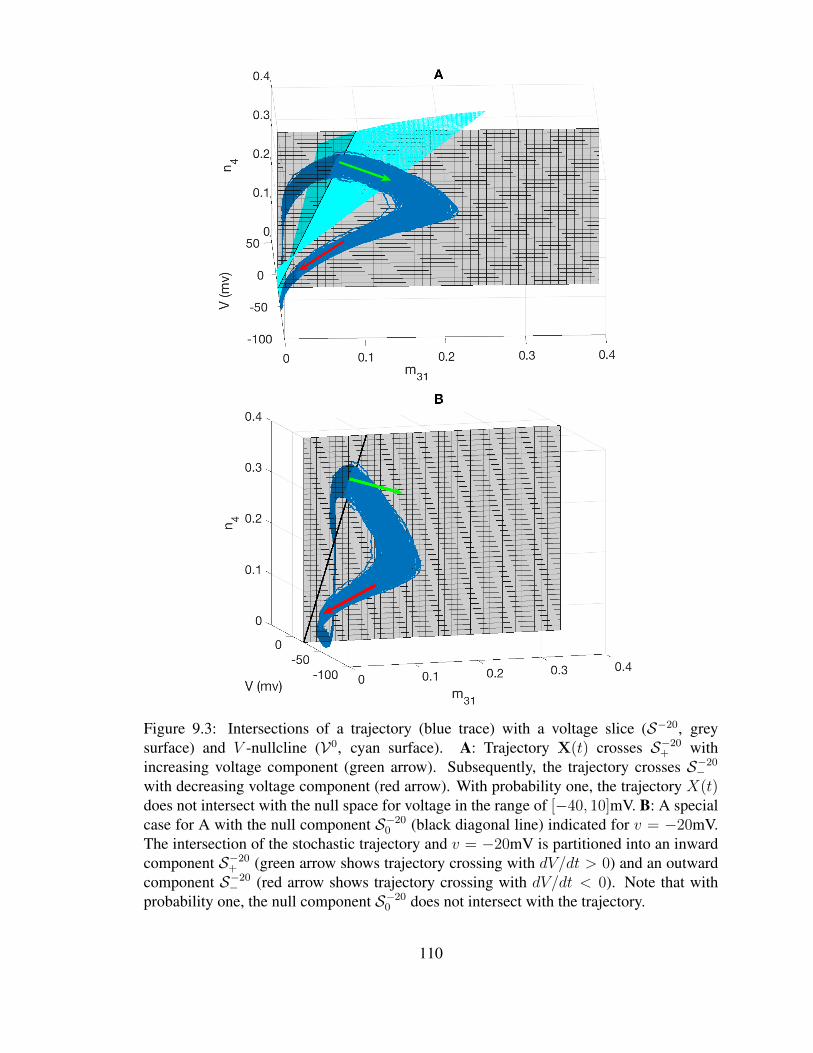
Figure 9.3: Intersections of a trajectory (blue trace) with a voltage slice (S−20, greysurface) and V -nullcline (V0, cyan surface). A: Trajectory X(t) crosses S−20+ withincreasing voltage component (green arrow). Subsequently, the trajectory crosses S−20−with decreasing voltage component (red arrow). With probability one, the trajectory X(t)does not intersect with the null space for voltage in the range of [−40, 10]mV. B: A specialcase for A with the null component S−200 (black diagonal line) indicated for v = −20mV.The intersection of the stochastic trajectory and v = −20mV is partitioned into an inwardcomponent S−20+ (green arrow shows trajectory crossing with dV/dt > 0) and an outwardcomponent S−20− (red arrow shows trajectory crossing with dV/dt < 0). Note that withprobability one, the null component S−200 does not intersect with the trajectory.
110
values of v, the density of trajectories in a neighborhood of V0 is very small for a finite
voltage range (here shown as −40 to +10 mV). Indeed for any u, the intersection of the
null set Su0 has measure zero relative to the uniform measure on Su, and the probability of
finding a trajectory at precisely V = u and dV/dt = 0 is zero. From this observation, and
because dV/dt is conditionally deterministic, given n, it follows that a trajectory starting
from x ∈ Su+ will necessarily cross Su− before crossing Su+ again (with probability one).
First-Passage Times Based on this observation, we can give a formal definition of the
first passage time as follows.
Definition 3. Given a section S ⊂ D, we define the first passage time (FPT) from a point
x ∈ D to S, for a stochastic conductance-based model as
τ(x,S)∆= inft > 0 |X(t) ∈ S &X(0) = x. (9.15)
Note that, more generally, we can think of τ as τ(x,S, ω), where ω is a sample from the
underlying Langevin process sample space, ω ∈ Ω.1 For economy of notation we usually
suppress ω, and may also suppress S, or x when these are clear from context.
In the theory of stochastic processes a stopping time, τ , is any random time such that
the event τ ≤ t is part of the σ-algebra generated by the filtration Ft of the stochastic
process from time 0 through time t. That is, one can determine whether the event defining
τ has occurred or not by observing the process for times up to and including t (see [89],
§7.2, for further details).
Remark 4. Given any section S ⊂ D and any point x ∈ D, the first passage time τ(x,S)
is a stopping time. This fact will play a critical role in the proof of our main theorem.1For the 14 × 28D Langevin Hodgkin-Huxley model, Ω may be thought of as the space of continuous
vector functions on [0,∞) with 28 components – one for each independent noise source.
111
As Figure 9.2 suggests, for −40 ≤ v ≤ +10 mV, the probability of finding trajectories
in an open neighborhood of Sv0 can be made arbitrarily small by making the neighborhood
around Sv0 sufficiently small. This observation has two important consequences. First,
because the probability of being near the nullcline Sv0 is vanishingly small, interspike
intervals are well defined (cf. Def. 5, below), even for finite precision numerical simulation
and trajectory analysis. In addition, this observation lets us surround the nullcline with a
small cylindrical open set, through which trajectories are unlikely to pass. This cylinder-
shaped buffer will play a role in defining the mean–return-time phase in §9.5.
Moreover, as illustrated in Figure 9.2, when V = −20mV, the stochastic trajectory x
intersects S−20 at two points within each full cycle, where one is in S−20+ and one in S−20− . In
addition, the trajectory crosses S−20− before it crosses S−20+ again. This is a particular feature
for conductance-based models in which dV/dt is conditionally deterministic, i.e. the model
includes no current noise.2
Definition 4. Given any set S ⊂ D (for instance, a voltage-section) and a point x ∈ D,
the mean first passage time (MFPT) from x to S,
T (x,S)∆= E[τ(x,S)], (9.16)
and the second moment of the first passage time is defined as
S(x,S)∆= E
[τ(x,S)2
]. (9.17)
2In this dissertation, we focus on a Langevin equation, rather than models with discrete channelnoise. Therefore, our trajectories are diffusions, that have continuous sample paths (with probability one).Therefore, the FPT τ(x,S) is well defined. For discrete channel-noise models, a slightly modified definitionwould be required.
112
Interspike Intervals Starting from x ∈ Sv0+ , at time t = 0, we can identify the sequence
of (τ,x) pairs of crossing times and crossing locations as
(τu0 = 0,xu0 = x), (τ d1 ,xd1), (τ
u1 ,x
u1), . . . , (τ dk ,x
dk), (τ
uk ,x
uk), . . . ,
with 0 = τu0 < τ d1 < τu1 < τ d2 < τu2 < . . . < τ dk < τuk , . . .
(9.18)
where τ dk = inft > τuk−1 | x ∈ Sv0− is the kth down-crossing time, xdk ∈ S
v0− is the kth
down-crossing location, τuk = inft > τ dk | x ∈ Sv0+ is the kth up-crossing time, and
xuk ∈ Sv0+ is the kth up-crossing location, for all k ∈ N+.
Under constant applied current, the HH system has a unique stationary distribution
with respect to which the sequence of crossing times and locations have well-defined
probability distributions [100].We define the moments of the interspike interval distribution
with respect to this underlying stationary probability distribution.
Definition 5. Given a sequence of up- and down-crossings, relative to a reference volt-
age v0 as above, the kth interspike interval (ISI), Ik (in milliseconds), of the stochastic
conductance-based model is a random variable that is defined as
Ik∆= τuk+1 − τuk (9.19)
where τuk is the kth up-crossing time. The mean ISI is defined as
I∆= E[Ik] (9.20)
and the second moment of the ISI is defined as
H∆= E
[I2k]
(9.21)
113
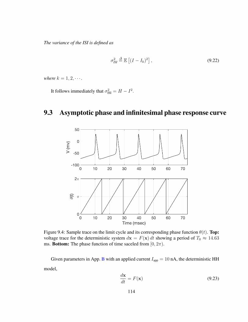
The variance of the ISI is defined as
σ2ISI
∆= E
[(I − Ik)2
], (9.22)
where k = 1, 2, · · · .
It follows immediately that σ2ISI = H − I2.
9.3 Asymptotic phase and infinitesimal phase response curve
Figure 9.4: Sample trace on the limit cycle and its corresponding phase function θ(t). Top:voltage trace for the deterministic system dx = F (x) dt showing a period of T0 ≈ 14.63ms. Bottom: The phase function of time saceled from [0, 2π).
Given parameters in App. B with an applied current Iapp = 10 nA, the deterministic HH
model,dx
dt= F (x) (9.23)
114
fires periodically with a period T0 ≈ 14.63 msec, as shown in Fig. 9.4. We assume that the
deterministic model has an asymptotically stable limit cycle, γ(t) = γ(t + T0). The phase
of the model at time t can be defined as [110]
θ(t) =(t+ T0
ϕ2π
) modT0T0
× 2π, (9.24)
where mod is the module operation, and θ(t) = 0 sets the spike threshold for the model.
The constant ϕ ∈ [0, 2π] is the relative phase determined by the initial condition, and there
is a one-to-one map between each point on the limit cycle and the phase. In general, the
phase can be scaled to any constant interval; popular choices include [0, 1), [0, 2π), and
[0, T ). Here we take θ ∈ [0, 2π) (see Fig. 9.4).
Winfree and Guckenheimer extended the definition of phase from the limit cycle to
the basin of attraction, which laid the foundation for the asymptotic phase function φ(x)
[54, 130, 131]. For the system in Eqn. (9.23), let x(0) and y(0) be two initial conditions,
one on the limit cycle and one in the basin of attraction, respectively. Denote the phase
associated to x(0) as θ0(t). If the solutions x(t) and y(t) satisfy
limt→∞|x(t)− y(t)| = 0, i.e. lim
t→∞|φ(y(t))− θ0(t)| = 0,
then y(0) has asymptotic phase θ0. The set of all points sharing the same asymptotic phase
comprises an isochron, a level set of φ(x). We also refer to such a set of points as an iso-
phase surface [109]. By construction, the asymptotic phase function φ(x) coincides with
the oscillator phase θ(t) on the limit cycle, i.e. θ(t) = φ(γ(t)). We will assume that φ(x)
is twice-differentiable within the basin of attraction.
The phase response curve (PRC) is defined as the change in phase of an oscillating
system in response to a given perturbations. If the original phase is defined as θb and the
115
phase after perturbation as θa, then the PRC is the shift in phase
∆(θ) = θa − θb.
In the limit of small instantaneous perturbations, the PRC may be approximated by the
infinitesimal phase response curve (iPRC) [110, 131]. For a deterministic limit cycle, the
iPRC Z(t) obeys the adjoint equation [11]
dZ
dt= −J (γ(t))ᵀZ, (9.25)
Z(0) = Z(T0), (9.26)
Z(0)ᵀF(γ(0)) = 1 (9.27)
where T0 is the period of the deterministic limit cycle, γ(t) is the periodic limit cycle
trajectory (for the HH equations (9.23), γ(t) ∈ R14) and J (t) = DF(γ(t)) is the Jacobian
of F evaluated along the limit cycle. The iPRC Z(t) is proportional to the gradient of the
phase function φ(x) evaluated on the limit cycle. For any point x in the limit cycle’s basin
of attraction, we can define a timing sensitivity function Z(x)∆= T0
2π∇xφ(x). For the limit
cycle trajectory γ(t), we have Z(t) = Z(γ(t)). The first component of Z, for example, has
units of msec/mv, or change in time per change in voltage.
9.4 Small-noise expansions
In the governing Langevin equation (6.42), the stochastic forcing components in G dW
are implicitly scaled by factors proportional to 1/√Nion, the number of sodium or potas-
sium channels in the membrane. The larger the number of channels, the smaller the
116
noise. In their comparative study of different Langevin models, Goldwyn and Shea-Brown
considered a patch of excitable membrane containing Mref = 6000 sodium channels and
Nref = 1800 potassium channels [49].
Here, we make the dependence on system size (number of channels) explicit, by in-
troducing a small parameter ε ∝ N−1ion . We therefore consider a one-parameter family of
Langevin equations,
dX = F(X) dt+√εG(X) dW(t), (9.28)
with effective numbers of Mtot = Mref/ε sodium and Ntot = Nref/ε potassium channels.
For sufficiently small values of ε, the solutions remain close to the determinstic limit cycle;
the (stochastic) interspike intervals will remain close to the deterministic limit cycle period
T 0. If X(t) is a trajectory of (9.28), and φ(x) is any twice-differentiable function, then
Ito’s lemma [89] gives an expression for the increment of φ during a time increment dt,
beginning from state X:
dφ(X(t)) = (∇φ(X)) · dX +ε
2
∑ij
∂2φ(X)
∂xi∂xjdt (9.29)
=
(F(X) · ∇φ(X) +
ε
2
∑ij
∂2φ(X)
∂xi∂xj
)dt+
√ε (∇φ(X))ᵀ G(X) dW
= L†[φ(X)] dt+√ε (∇φ(X))ᵀ G(X) dW (9.30)
up to terms of order dt. The operator L† defined by (9.29)-(9.30) is the formal adjoint of the
Fokker-Planck or Kolmogorov operator [99], also known as the generator of the Markov
process [89], or the Koopman operator [72].
Dynkin’s formula, which we will use to prove our main result, is closely related to
equation (9.30). Let x ∈ D and let Ex denote the probability law for the ensemble of
117
stochastic trajectories beginning at x. Dynkin’s theorem ([89], §7.4) states that if φ is a
twice-differentiable function on D, and if τ is any stopping time (cf. Remark 4) such that
Ex[τ ] <∞, then
Ex[φ(X(τ)] = φ(x) + Ex
[∫ τ
0
L†[φ(X(s)] ds
]. (9.31)
9.5 Iso-phase Sections
For the deterministic model, the isochrons form a system of Poincare sections Sϕ, ϕ ∈
[0, 2π], each with a constant return time equal to the oscillator period T0. When the system
is perturbed by noise, ε > 0 in (9.28), we consider a set of “iso-phase sections” based on
a mean–return-time (MRT) construction, first proposed by [109] and rigorously analyzed
by [75]. As shown in [75], the MRT iso-phase surfaces S are the level sets of a function
Tε(x) satisfying the MRT property. Namely, if S is an iso-phase section, then the mean
time taken to return to S, starting from any x ∈ S, after one full rotation, is equal to the
mean period, T ε.
The construction in [75] requires that the Langevin equation (9.28) be defined on a
domain with the topology of an n-dimensional cylinder, because finding the MRT function
Tε(x) involves specifying an arbitrary “cut” from the outer to the inner boundary of the
cylinder. Conductance-based models in the steady-firing regime, where the mean-field
equations support a stable limit cycle, can be well approximated by cylindrical domains. In
particular, their variables are restricted to a compact range, and there is typically a “hole”
through the domain in which trajectories are exceedlingly unlikely to pass, at least for small
noise.
As an example, consider the domain for the 14D HH equations (recall Defs. 1), namely
118
D ∆= [vmin, vmax] × ∆7 × ∆4. The p-dimensional simplex ∆p is a bounded set, and, as
established by Lemma 1, the trajectories of (9.28) remain within fixed voltage bounds with
probability 1, so our HH system operates within a bounded subset of R14. To identify a
“hole” through this domain, note that the set
Su0∆= Su ∩ V0 = (v,m,n) ∈ D | v = u & f(v,m,n) = 0 ,
which is the intersection of the voltage nullcline V0 with the constant-voltage section Su,
is rarely visited by trajectories under small noise conditions (Fig. 9.2B).
For r > 0, we define the open ball of radius r around Su0 as
Br(Su0 )∆=
x ∈ D
∣∣∣ miny∈Su0
(||x− y||) < r
. (9.32)
For the remainder of the thesis, we take the stochastic differential equation (9.28) to be
defined on
D0 = D\Br(Sv0 ). (9.33)
For sufficiently small r > 0, D0 is a space homeomorphic to a cylinder in R14. To see this,
consider the annulus A = I1 × B13, where I1 = [0, 2π], and B13 is a simply connected
subset of R13. That space is homotopy equivalent to a circle S1 by contracting the closed
interval parts to a point, and contracting the annulus part to its inner circle.
To complete the setup so that we can apply the theory from [75], we set boundary
conditions∑
ij ni(GGᵀ)ij∂jTε = 0 at reflecting boundaries with outward normal n on both
the innner and outer boundaries of the cylinder. In addition, we choose an (arbitrary)
section transverse to the cylinder, and impose a jump condition Tε → Tε + T ε across
this section, where T ε is mean oscillator period under noise level ε.
119
As showed in [75], this construction allows us to establish a well defined MRT function
for a given noise level ε, T ε(x). We then obtain the iso-phase sections as level sets of T ε(x).
We give a formal definition as follows.
Definition 6. Given a fixed noise level ε ≥ 0, and an iso-phase surface S for eqn. (9.28),
we define the kth iso-phase interval (IPI) as the random variable
∆k∆= µk − µk−1, (9.34)
where µkk∈N+ is a sequence of times at which the trajectory crosses S. The mean IPI is
defined as
T ε∆= E[∆k] (9.35)
and the second moment of the IPI is defined as
Sε∆= E
[∆2k
]. (9.36)
The variance of the IPI is defined as
σ2φ∆= E
[(T ε −∆k)
2]. (9.37)
The moments (9.35)-(9.37) are evaluated under the stationary probability distribution.
It follows immediately that for a given noise level ε, we have σ2φ = Sε −∆2
ε .
Remark 5. Each iso-phase crossing time, µkk∈N+ , in Definition 6, is a stopping time.
Remark 6. Because (9.28) is a diffusion with continuous sample paths, it is possible that
when ε > 0 a stochastic trajectory X(t) may make multiple crossings of an iso-phase
120

section S in quick succession. Should this be the case, we condition the crossing times µk
on completion of successive circuits around the hole in our cylindrical domain. That is,
given µk, we take µk+1 to be the first return time to S after having completed at least one
half a rotation around the domain.
121
Chapter 10
Noise Decomposition of the 14-D
Stochastic HH Model
Ermentrout et al. [31] studied the variance of the infinitesimal phase response curve for a
neuronal oscillator driven by a white noise current, using a four-dimensional version of the
Hodgkin-Huxley model as an example. As a corollary result, they obtained an expression
for the variance of the interspike interval, by setting the size of the perturbing voltage pulse
to zero.
Stochastic shielding [102] allows one to resolve the molecular contributions (per di-
rected edge in the ion channel state transition graph E , cf. Fig. 3.1) to the variance of
ion channel currents [104, 105], and provides a numerical method for accurate, efficient
simulation of Langevin models using a small subset of the independent noise forcing (only
for the “most important edges”) [95].
Here we combine the stochastic shielding method with Cao et al.’s mean–return-time
phase analysis [75] to obtain an analytical decomposition of the molecular sources of timing
122
variability under current clamp.
Prior analysis of stochastic shielding ( [104, 105]) assumed voltage clamp conditions,
under which the ion channel state process is a stationary Markov process. Under current
clamp, however, fluctuations of channel state determine fluctuations in current, which in
turn dictate voltage changes, which then influence channel state transition probabilities,
forming a closed loop of statistical interdependence. Therefore, the variance of ISI under
current clamp becomes more difficult to analyze. Nevertheless, in this section, we seek
a decomposition of the interspike-interval variance into a sum of contributions from each
edge k ∈ E , e.g.
σ2ISI(ε) = ε
∑k∈E
σ2ISI,k +O(ε2) (10.1)
σ2φ(ε) = ε
∑k∈E
σ2φ,k +O(ε2) (10.2)
to leading order as ε→ 0.
Theorem 4 below gives the detailed form of the decomposition. As preliminary evi-
dence for its plausibility, Fig. 10.1 shows the coefficient of variation (standard deviation
divided by mean) of the ISI under the stochastic shielding approximation for Langevin
model in different scenarios: including noise along a single directed edge at a time (blue
bars), or on edges numbered 1 to k inclusive (numbering follows that in Fig. 3.1). For
large noise (Fig. 10.1a,c), the effects of noise from different edges combine subadditively.
For small noise (Fig. 10.1b,d) contributions of distinct edges to firing variability combine
additively. Edges with small contribution to steady-state occupancy under voltage clamp
(edges 1-6 for K+, edges 1-18 for Na+, cf. Fig. 3.1) contribute additively even in the large-
noise regime. Thus even in the large-noise regime, stochastic shielding allows accurate
simulation of ISI variability using significantly fewer edges for both the sodium and potas-
123
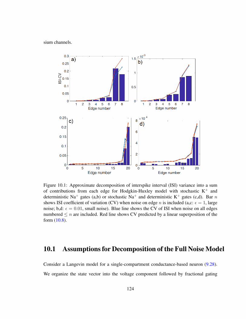
sium channels.
Figure 10.1: Approximate decomposition of interspike interval (ISI) variance into a sumof contributions from each edge for Hodgkin-Huxley model with stochastic K+ anddeterministic Na+ gates (a,b) or stochastic Na+ and deterministic K+ gates (c,d). Bar nshows ISI coefficient of variation (CV) when noise on edge n is included (a,c: ε = 1, largenoise; b,d: ε = 0.01, small noise). Blue line shows the CV of ISI when noise on all edgesnumbered ≤ n are included. Red line shows CV predicted by a linear superposition of theform (10.8).
10.1 Assumptions for Decomposition of the Full Noise Model
Consider a Langevin model for a single-compartment conductance-based neuron (9.28).
We organize the state vector into the voltage component followed by fractional gating
124
variables as follows:
x = (v, q1, q2, . . . , qN)ᵀ. (10.3)
Here, N is the number of nodes in the union of the ion channel state graphs. For example,
for the HH system, N = 13, and we would write q1 = m00, . . . , q8 = m31 for the sodium
gating variables, and q9 = n0, . . . , q13 = n4 for the potassium gating variables. Similarly,
we enumerate the K edges occurring in the union of the ion channel state graphs, and write
the stoichiometry vector ζk ∈ RN+1 for transition k, taking source i(k) to destination j(k),
in terms of (N + 1)-dimensional unit vectors eN+1i ∈ RN+1 as ζk = −eN+1
i(k) + eN+1j(k) . In
order to study the contributions of individual molecular transitions to spike-time variability,
we develop asymptotic expansions of the first and second moments of the distribution of
iso-phase surface crossing times (iso-phase interval distribution see Def. 6 above) in the
small ε limit.
Before formally stating the theorem, we make the following assumptions concerning
the system (9.28):
A1 We assume the deterministic dynamical system dXdt
= F(x) has an asymptotically,
linearly stable limit cycle x = γ(t) with finite period T0, and asymptotic phase func-
tion φ(x) defined throughout the limit cycle’s basin of attraction such that dφ(x(t))dt
=
2πT0
along deterministic trajectories, and a well defined infinitesimal phase response
curve (iPRC), Z(t) = ∇φ(γ(t)).
A2 We assume that the (N + 1)×K matrix G has the form
G(x) =K∑k=1
(ζkrk)√αk(v)qi(k) (10.4)
where rk =(eKk)ᵀ is an K-dimensional unit row vector with all zero components
125
except in the kth entry, αk(v) is the voltage-dependent per capita transition rate along
the kth directed edge, and the qi(t) denote channel state occupancy probabilities as
described above (cf. (10.3)).
Remark 7. The product ζkrk is a (N + 1)×K sparse matrix, containing zeros everywhere
except in the kth column. Each column conveys the impact of an independent noise source
on the state vector [95].
A3 We assume that for sufficiently small noise, 0 < |ε| 1, we have a well defined
joint stationary probability distribution in the voltage V and the gating variables
Q1, . . . , QN with a well defined mean period T ε and mean–return-time phase func-
tion Tε(x). Moreover, we assume that the mean period, the MRT function, and the
second moment function all have well defined series expansions:
T ε = T 0 + εT 1 +O(ε2) (10.5)
Tε(x) = T0(x) + εT1(x) +O(ε2) (10.6)
Sε(x) = S0(x) + εS1(x) +O(ε2), (10.7)
as ε→ 0.
Remark 8. Note that the expansions (10.5)-(10.7) may break down in the small-ε limit for
noise-dependent oscillators, such as the heteroclinic oscillator [121] or ecological quasi-
cycles [80], but should remain valid for finite-period limit cycles such as the Hodgkin-
Huxley system in the periodic spiking regime.
126
10.2 Noise Decomposition Theorem
Theorem 4 (Noise Decomposition Theorem). Let x = (V0,Q0) ∈ S0 be the point on the
deterministic limit cycle such that φ(x) = 0 (i.e. assigned to “phase zero”), and let Ex
denote expectation with respect to the law of trajectories with initial condition x, for fixed
ε ≥ 0. Under assumptions A1-A3, the variance σ2φ of the S0-isochron crossing times (iso-
phase intervals, or IPI) for conductance-based Langevin models (eqn. (6.42)) decomposes
into additive contributions from each channel-state transition, in the sense that
σ2φ =
∑k∈all edges
σ2φ,k (10.8)
=ε∑k
∫ T 0
0
Ex
(αk(V (t))Qi(k)(t)
(ζᵀk Z(X(t))
)2)dt+O
(ε2), (10.9)
as ε→ 0+. The function X(t) = (V (t), Q1(t), . . . , QN(t))ᵀ denotes a stochastic trajectory
of (9.28) with initial condition x.
Remark 9. The theorem holds independently of the choice of the initial point x on the
deterministic limit cycle, in the sense that choosing a different base point would just shift
the endpoints of the interval of integration; since the deterministic limit cycle is periodic
with period T 0, the resulting expression for σ2φ is the same. See Corollary 7.
Remark 10. The proof relies on Dynkin’s formula, first–passage-time moment calcula-
tions, and a small noise expansion. The right hand side of (10.8) leads to an approximation
method based on sampling stochastic limit cycle trajectories, which we show below gives
an accurate estimate for σ2φ.
Remark 11. Although the interspike intervals (ISI) determined by voltage crossings are not
strictly identical to the iso-phase intervals (IPI) defined by level crossings of the function
127
Tε(x), we nevertheless expect that the variance of the IPI, and their decomposition, will
provide an accurate approximation to the variance of the ISI. In §11 we show numerically
that the decomposition given by (10.8) predicts the contribution of different directed edges
to the voltage-based ISIs with a high degree of accuracy.
Before proving the theorem, we state and prove two ancillary lemmas.
Lemma 5. Fix a cylindrical domainD0 (as in equation (9.33)) and an iso-phase section S0
transverse to the vector field F. If the mean period T ε and MRT function Tε(x) have Taylor
expansions (10.5) and (10.6), then the unperturbed isochron function T0 and the sensitivity
of the isochron function to small noise T1 satisfy
F(x) · ∇T0(x) = −1, (10.10)
F(x) · ∇T1(x) = −1
2
∑ij
(GGᵀ)ij∂2ijT0(x), (10.11)
∑ij
ni(GGᵀ)ij∂jT1
∣∣∣∣∣∂D
= 0, (10.12)
where T1 → T1 + T 1 and T0 → T0 + T 0 across S0, and n is the outward normal to the
boundary ∂D.
Note that T 1 may be determined from the stationary solution of the forward equation
for 0 < ε, or through Monte Carlo simulations (in some cases T 1 ≡ 0).
Proof. For all noise levels ε ≥ 0, from [43] (Chapter 5, equation 5.5.19), the MRT function
Tε(x) satisfies
L† [Tε] = F · ∇Tε +ε
2
∑ij
(GGᵀ)ij∂2ijTε = −1, (10.13)
together with adjoint reflecting boundary conditions at the edges of the domain D with
128
outward normal vector n
∑ij
ni(GGᵀ)ij∂jTε
∣∣∣∣∣∂D
= 0 (10.14)
and the jump condition is specified as follows. When x increases across the reference
section S in the “forward direction”, i.e., in a direction consistent with the mean flow in
forwards time, the function Tε → Tε + T ε. Note that since T0 → T0 + T 0, we also have
T1 → T1 + T 1 across the same Poincare section, for consistency.
Substituting the expansion (10.6) into (10.13) gives
−1 =F · ∇(T0(x) + εT1(x) +O(ε2)
)+ε
2
∑ij
(GGᵀ)ij∂2ij(T0(x) + εT1(x) +O(ε2)
),
(10.15)
=F · ∇T0(x) + F · ∇(εT1(x) +O(ε2)
)+ε
2
∑ij
(GGᵀ)ij∂2ijT0(x) (10.16)
+ε
2
∑ij
(GGᵀ)ij∂2ij(εT1(x) +O(ε2)
)Note that, when ε = 0
F · ∇T0(x) = −1, (10.17)
consistent with T0 being equal to minus the asymptotic phase of the limit cycle (up to an
additive constant). On the other hand, for ε 6= 0, by comparing the first order term, the
sensitivity of the isochron function to small noise T1 satisfies
F · ∇T1(x) = −1
2
∑ij
(GGᵀ)ij∂2ijT0,∑ij
ni(GGᵀ)ij∂jT1
∣∣∣∣∣∂D
= 0, (10.18)
where T1 → T1 + T 1 across S, and n is the outward normal to the boundary ∂D, thus we
129
proved Lemma 5.
Our next lemma concerns the second moment of the first passage time from a point
x ∈ D to a given iso-phase section S0, that is, Sε(x)∆= E [τ(x,S0)2], cf. (9.17).
Lemma 6. Suppose the assumptions of Lemma 5 hold, and assume in addition that Sε has
a Taylor expansion (10.7) for small ε. The second moment, S0(x), of the first passage time
τ(X,S) from a point x to a given isochron section S0 = Tε(x) = const, and its first
order perturbation, S1(x), satisfy
F · ∇S0 = −2T0 (10.19)
F · ∇S1 +1
2
∑ij
(GGᵀ)ij∂2ijS0 = −2T1. (10.20)
Proof. Following [43] (Chapter 5, equation 5.5.19), the second moment Sε(x) of the first
passage time from a point x to a given isochron Tε(x) = const, satisfies
L†[Sε] := F · ∇Sε +ε
2
∑ij
(GGᵀ)ij∂2ijSε = −2Tε.
Substituting in the Taylor expansions (10.5)-(10.7), we have to order O(ε)
F · ∇(S0 + εS1) +ε
2
∑ij
(GGᵀ)ij∂2ij(S0 + εS1) = −2(T0 + εT1) +O(ε2). (10.21)
Setting ε = 0, we see that
F · ∇S0 = −2T0. (10.22)
130
For ε > 0, the first order terms yield
F · ∇S1 +1
2
∑ij
(GGᵀ)ij∂2ijS0 = −2T1. (10.23)
Therefore, we complete the proof of Lemma 6.
10.3 Proof of Theorem 4
Proof. We divide the proof of the Theorem into three steps.
1. First, we will calculate the infinitesimal generator for the variance of the iso-phase
interval (IPI).
For fixed noise level ε > 0, the variance of IPI, σ2φ is equal to the expected value of
Vε = Sε − T 2ε , evaluated at the isochron T = const + T . Note that when ε = 0, the
system is deterministic and the iso-phase interval has a zero variance, i.e., V0 ≡ 0.
Expanding Sε = S0 + εS1 +O(ε2) and Vε = εV1 +O(ε2) to first order in ε 1, then
Vε = V0 + εV1 +O(ε2) (10.24)
= Sε − T 2ε (10.25)
= S0 + εS1 +O(ε2)−(T0(x) + εT1(x) +O(ε2)
)2 (10.26)
= S0 − T 20 + ε(S1 − 2T0T1) +O(ε2), (10.27)
thus,
S0 = T 20 (10.28)
S1 = V1 + 2T0T1. (10.29)
131
Plug the above results into equation (10.23) (Lemma 6), we can obtain that
F · ∇(V1 + 2T0T1) +1
2
∑ij
(GGᵀ)ij∂2ijT 20 = −2T1. (10.30)
By the product rule and use equations (10.17), and (10.18),
F · ∇(2T0T1) = 2T1F · ∇(T0) + 2T0F · ∇(T1) (10.31)
= −2T1 − T0∑ij
(GGᵀ)ij∂2ijT0. (10.32)
Therefore,
F · ∇V1 − 2T1 − T0∑ij
(GGᵀ)ij∂2ijT0 +1
2
∑ij
(GGᵀ)ij∂2ijT 20 = −2T1. (10.33)
Since ∂2ijT20 = ∂i(2T0∂jT0) = 2∂iT0∂jT0 + 2T0∂
2ijT0, it follows that
F · ∇V1 − T0∑
ij(GGᵀ)ij∂2ijT0 +∑
ij(GGᵀ)ij∂iT0∂jT0 +∑
ij(GGᵀ)ijT0∂2ijT0 = 0
F · ∇V1 = −∑
ij(GGᵀ)ij∂iT0∂jT0 (10.34)
Finally,
L†[Vε] = L†[V0 + εV1 +O(ε2)] (10.35)
= εL†[V1] +O(ε2) (10.36)
= ε
(F · ∇V1 +
ε
2
∑ij
(GGᵀ)ij∂2ijV1
)+O(ε2) (10.37)
= ε (F · ∇V1) +O(ε2) (10.38)
= −ε∑ij
(GGᵀ)ij∂iT0∂jT0 +O(ε2), (10.39)
132
where we used V0 ≡ 0 and applied equation (10.34).
2. Secondly, we will show that for first-order transition networks underlying the molec-
ular ion channel process, the decomposition GGᵀ =∑
k∈E GkGᵀk is exact.
To see this, note that G can be written as a sum of 29 sparse matrix with one zero
matrix and 28 rank one matrix. The kth rank one matrix consists of the transition due
to the kth edge and there are 28 edges in the 14-D HH model. The kth column of
the kth rank one matrix equals to a stoichiometry vector times the square root of the
corresponding state occupancy and zeros otherwise. For example, the kth column of
G is given by
Gk = ζk
√αk(v)Xi(k),
where ζk is the stoichiometry vector, αk is the voltage-dependent per capita transi-
tion rate, and Xi(k) is the population vector component at the source node i(k) for
transition number k.
GGᵀ = (G1 + G2 + · · ·+ G28)(G1 + G2 + · · ·+ G28)ᵀ (10.40)
=28∑k=1
GkGᵀk (10.41)
=28∑k=1
αk(v)Xi(k)ζkζᵀk (10.42)
where (10.41) holds because GiGᵀj = 0 when i 6= j.
Note that ∂iT0∂jT0 = ω−2∂iφ(x)∂jφ(x) = Zi(x)Zj(x), with ω ≡ 2π/T 0, because φ
133
is normalized to range from 0 to 2π, and T0 ranges from 0 to T 0.
∑ij
(GGᵀ)ij∂iT0∂jT0 =∑ij
(GGᵀ)ijZiZj (10.43)
=29∑k=2
∑ij
(GkGᵀk)ijZiZj (10.44)
=28∑k=1
(αk(v)Xi(k)
∑ij
(ζkζᵀk )ijZiZj
)(10.45)
=28∑k=1
αk(v)Xi(k)
[Z2i(k) + Z2
j(k) − 2Zi(k)Zj(k)]
(10.46)
=28∑k=1
αk(v)Xi(k)
[Zi(k) − Zj(k)
]2 (10.47)
=28∑k=1
αk(v)Xi(k)
(ζᵀk Z
)2, (10.48)
where i(k) and j(k) are the source and sink nodes for transition number k. Equation
(10.46) holds because the kth edge only involves two nodes.
3. Finally, we will apply Dynkin’s formula to complete the rest of the proof.
For a stopping time τ(x) with Ex (τ) <∞, by Dynkin’s formula (9.31), the expected
IPI variance starting from x is
Ex (Vε(X(τ))) = Vε(x) + Ex
(∫ τ
0
L†[Vε(X(s))]ds
)(10.49)
The first return time τ is the time at which the trajectory X(t) first returns to the
isochron S0, therefore X(τ) ∈ S0 and the time left to reach S0 from the random
location X(τ) is guaranteed to be zero. That is, Vε(X(τ)) = 0 with probability 1.
Hence, Ex (Vε(X(τ))) ≡ 0 for all x ∈ S0.
134
Fix a mean–return-time isochron S0, the mean return time from any initial location
x ∈ S0 back to S0, after completing one rotation is exactly T ε, by construction.
However, in principle, the variance of the return time might depend on the initial
location within the isochron. We next show that, to leading order in ε, this is not the
case, that is, the MRT isochrons have uniform first and second moment properties.
Using equations (10.39), (10.48) and (10.49), we obtain
Vε(x) = −Ex
(∫ τ
0
L† [Vε(X(s))] ds
)(10.50)
= Ex
(∫ τ
0
ε∑ij
(GGᵀ)ij∂iT0∂jT0ds
)+O
(ε2)
(10.51)
= ε28∑k=1
Ex
(∫ τ
0
αk(v)Xi(k)
(ζᵀk Z
)2ds
)+O
(ε2), (10.52)
where the integrals are evaluted along a stochastic trajectory X(t) with X(0) = x
and X(τ) ∈ S0, one rotation later. Holding the deterministic zero-phase isochron S0
fixed, and choosing an arbitrary point y ∈ D, we have, by definition,
Ey[τ(y)] = Tε(y) = T0(y) + εT1(y) +O(ε2). (10.53)
Therefore, starting from an initial condition x ∈ S0 one period earlier, we have
Ex
(∫ τ
0
αk(v)Xi(k)
(ζᵀk Z
)2ds
)= Ex
(∫ T 0
0
αk(v)Xi(k)
(ζᵀk Z
)2ds
)+O
(ε2).
(10.54)
135
This relation follows immediately from our assumptions, because, for x ∈ S0,∣∣∣∣∣Ex
(∫ τ
0αk(V (s))Xi(k)(s)
(ζᵀk Z(s)
)2ds
)− Ex
(∫ T 0
0αk(V (s))Xi(k)(s)
(ζᵀk Z(s)
)2ds
)∣∣∣∣∣=
∣∣∣∣Ex
(∫ τ
T 0
αk(V (s))Xi(k)(s)(ζᵀk Z(s)
)2ds
)∣∣∣∣ (10.55)
≤ C1
∣∣Ex(τ(x)− T 0)∣∣ = C1
∣∣Ex(τ(x))− Ex(T 0)∣∣ = C1
∣∣T ε − T 0
∣∣ (10.56)
= εC1T 1 +O(ε2). (10.57)
Here C1 is a positive constant bounding the integrand αk(v(t))Xi(k)(t)(ηᵀkZ(t)
)2.
From Remark 3, αk ≤ αmax. By definition, 0 ≤ Xi ≤ 1 for each i. For each edge
k, |ζk| =√
2. Since Z is continuous and periodic, |Z| is bounded by some constant
zmax. Therefore setting C1 =√
2αmaxzmax satisfies (10.57).
Because the initial point x ∈ S0 was located at an arbitrary radius along the specified
mean–return-time isochron, the calculation above shows that σ2φ = E[Vε(x) |x ∈ S0]
is uniform across the isochron S0, to first order in ε. Thus, for small noise levels,
the MRT isochrons enjoy not only a uniform mean return time, but also a uniform
variance in the return time, at least in the limit of small noise.
Finally, we note that σ2φ (equivalently, and Vε(x)) combine a sum of contributions
over a finite number of edges. From equations (10.52) and (10.54), the variance of
the inter-phase interval is given by
σ2φ = ε
28∑k=1
Ex
(∫ T 0
0
αk(V (s))Xi(k)(s)(ζᵀk Z(s)
)2ds
)+O
(ε2). (10.58)
136
To complete the proof, note that (10.9) follows from (10.59) by exchange of expec-
tation Ex[·] with (deterministic) integration∫ T 0
0[·] dt. This completes the proof of
Theorem 4.
The choice of the initial reference point x or isochron S0 in (10.59) was arbitrary and
the variance of IPI is uniform to the first order. Therefore, the inter-phase-interval variance
may be uniform (to first order) almost everywhere in D. We can then replace the integral
around the limit cycle in (10.59) with an integral over D with respect to the stationary
probability distribution. Thus we have the following
Corollary 7. Under the assumptions of Theorem 4, the inter-phase-interval variance sat-
isfies
σ2φ = εT 0
28∑k=1
E(αk(V )Xi(k)
(ζᵀk Z(X)
)2)+O
(ε2), (10.59)
as ε → 0, where E denotes expectation with respect to the stationary probability density
for (9.28).
Remark 12. Because the variance of the IPI, σ2φ, is uniform regardless the choice of the
reference iso-phase section, we will henceforth refer it as σ2IPI throughout the rest of this
thesis.
Now we can say we have generalized the edge important measure introduced in [105]
for the voltage-clamp case to the current clamp case with weak noise. In the next chapter
we leverage Theorem 4 to estimate the inter-phase interval variance in two different ways:
by averaging over one period of the deterministic limit cycle (compare (10.58)) or by
averaging over a long stochastic simulation (compare (10.59)). As we will see below,
137

both methods give excellent agreement with direct measurement of the inter-phase interval
variance.
138
Chapter 11
Decomposition of the Variance of
Interspike Intervals
Theorem 4 and Corollary 7 assert that for sufficiently weak levels of channel noise, the
contributions to inter-phase interval variance made by each individual edge in the channel
state transition graph (cf. Fig. 3.1) combine additively. Moreover, the relative sizes of these
contributions provide a basis for selecting a subset of noise terms to include for running
efficient yet accurate Langevin simulations, using the stochastic shielding approximation
[95]. In this chapter, we test and illustrate several aspects of these results numerically.
First, we confront the fact that the inter-phase-intervals and the inter-spike-intervals are
not equivalent, since iso-voltage surfaces do not generally coincide with isochronal surfaces
[128]. Indeed, upon close examination of the ISI variance in both real and simulated
nerve cells, we find that the voltage-based σ2ISI is not constant, as a function of voltage,
while the phase-based σ2IPI remains the same regardless of the choice of reference isochron.
Nevertheless, we show that the voltage-based ISI variance is well approximated – to within
139
a few percent – by the phase-based IPI variance, and therefore, the linear decomposition of
Theorem 4 approximately extends to the ISI variance as well.
Second, after showing that the linear decomposition of the ISI variance holds at suf-
ficiently small noise levels, we explore the range of noise levels over which the linear
superposition of edge-specific contributions to ISI variance holds. Consistent with the basic
stochastic shielding phenomenon, we find that the variability resulting from noise along
edges located further from the observable transitions scales linearly with noise intensity, ε
even for moderate noise levels, while the linear scaling of eqn. (10.58) breaks down sooner
with increasing noise for edges closer to observable transitions.
Finally, we explore the accuracy of a reduced representation using only the two most
important edges from the K+channel and the four most important edges from the Na+channel,
over a wide range of noise intensities. Here, we find that removing the noise from all but
these six edges still gives an accurate representation of the ISI variance far beyond the weak
noise regime, despite the apparent breakdown of linearity.
In this section, the variance of ISIs and IPIs are calculated to compare with the pre-
dictions using Theorem 4. First, we numerically show that there is a small-noise region
within which Theorem 4 holds, for each individual edge, as well as for the whole Langevin
model (cf. (9.28)). We have two numerical approaches to evaluating the theoretical con-
tributions. The first method involves integrating once around the deterministic limit cycle
while evaluating the local contribution to timing variance at each point along the orbit.
This approach derives from the theorem, cf. (10.9) or (10.58), which we refer as the
“limit cycle prediction”. The second approach derives from the corollary, (10.59): we
average the expected local contribution to timing variation over a long stochastic trajectory.
More specifically, equation (10.59) gives a theoretical value of the average leading-order
140
contribution mass function, Pk, for the kth edge, as
Pk := E[αk(V )Xi(k)
(ζᵀk Z(X)
)2], (11.1)
where E(·) is the mean with respect to the stationary probability distribution of the stochas-
tic limit cycle. Given a sample trajectory X(t), we approximate the iPRC near the limit
cycle, Z(X(t)), by using the phase response curve of the deterministic limit cycle
Z(X(t)) ≈ Z(X(t))∆= Z
(argmin
s
∣∣∣∣(γ(s)−X(t)
)ᵀZ(s)
∣∣∣∣) , (11.2)
where γ is a point on the deterministic limit cycle and Z is the infinitesimal phase response
curve on the limit cycle (cf. §9.3). The predicted contribution of the kth edge to the IPI
variance with average period T0, is therefore
From Corollary 7 we have
σ2IPI ≈ εT 0
∑k
Pk. (11.3)
We call Pk the point mass prediction for the contribution of the kth edge to the inter-phase
interval variance.
For small noise, both approaches give good agreement with the directly measured IPI
variance, as we will see in Fig. 11.3.
To numerically calculate the contribution for each directed transition in Fig. 3.1, we
apply the stochastic shielding (SS) technique proposed by [102], simulating the Langevin
process with noise from all but a single edge suppressed. Generally speaking, the SS
method approximates the Markov process using fluctuations from only a subset of the
transitions, often the observable transitions associated to the opening states. Details about
how stochastic shielding can be applied to the 14 × 28D Langevin model is discussed in
141
§6.5.
All numerical simulations for the Langevin models use the same set of parameters,
which are specified in Tab. B.1 with given noise level ε in eqn. (9.28). We calculate
the following quantities: the point mass prediction Pk, using exact stochastic trajectories
(11.1); the predicted contributions by substituting the stochastic terms in (10.58) with the
deterministic limit cycle; the variance and standard deviation of the interspike intervals
(σ2ISI); and the variance and standard deviation of the isophase intervals (σ2
IPI).
In addition to numerical simulations, we will also present several observations of ex-
perimental recordings. Data in Fig. 11.1 and Fig. 11.2 were recorded in vitro in Dr. Friel’s
lab from intact wild type Purkinje cells with synaptic input blocked, with voltage sampled
at 20KHz and digitized at 1/32 mV resolution. We analyzed fourteen different voltage
traces from cerebellar Purkinje cells from wild type mice, and seventeen from mice with
the leaner mutation. The average number of full spike oscillations is roughly 1200 for wild
type PCs (fourteen cells) and 900 for leaner mutation (seventeen cells).
11.1 Observations on σ2ISI, and σ2
IPI
When analyzing voltage recordings from in vitro Purkinje cells (PCs) and from simulation
of the stochastic HH model, we have the following observations. First, given a particular
(stochastic) voltage trace, the number of interspike intervals (cf. Def. 5) varies along with
the change in voltage threshold used for identifying spikes. Second, within a range of
voltage thresholds for which the number of ISIs is constant, the variance of the inter-
spike interval distribution, σ2ISI (cf. Def. 5), which is obtained directly from the voltage
recordings, nevertheless varies as a function of the threshold used to define the spike times.
Thus the ISI variance, a widely studied quantity in the field of computational neuroscience
142
[57, 74, 86, 112, 118], is not invariant with respect to the choice of voltage threshold.
To our knowledge this observation has not been previously reported in the neuroscience
literature.1
Fig. 11.1 plots the histogram of voltage from a wild type PC and number of spikes cor-
responding to voltage threshold (Vth) in the range of [−60,−10] mV. Setting the threshold
excessively low or high obviously will lead to too few (or no) spikes. As the threshold
increases from excessively low values, the counts of threshold-crossing increases. For
example, when Vth is in the after hyper-polarization (AHP) range (roughly −58 . Vth .
−48 mV in Fig. 11.1) the voltage trajectory may cross the threshold multiple times before
it finally spikes. As illustrated in Fig. 11.1, the number of spikes is not a constant as
the threshold varies, therefore, the mean and variance of ISI are not well-defined in the
regions where extra spikes are counted. To make the number of spikes accurately reflect the
number of full oscillation cycles, in what follows we will only use thresholds in a voltage
interval that induces the correct number of spikes. Note that, for a given voltage trace and
duration (Ttot), if two voltage threshold generate the same number of spikes (Nspike), the
mean ISI would be almost identical, approximately Ttot/Nspike. This observation holds for
both experimental recordings and numerical simulations.
Next we address the sensitivity of the interspike interval to the voltage threshold, within
the range over which the number of ISIs is invariant.
From the earliest days of quantitative neurophysiology, the extraction of spike timing
information from voltage traces recorded via microelectrode has relied on setting a fixed
voltage threshold (originally called a Schmitt trigger, after the circuit designed by O.H.
Schmitt [106]). To our knowledge, it has invariably been assumed that the choice of the
1Throughout this section, we use the term “threshold” in the data analysis sense of a Schmitt trigger [106],rather than the physiological sense of a spike generation mechanism.
143
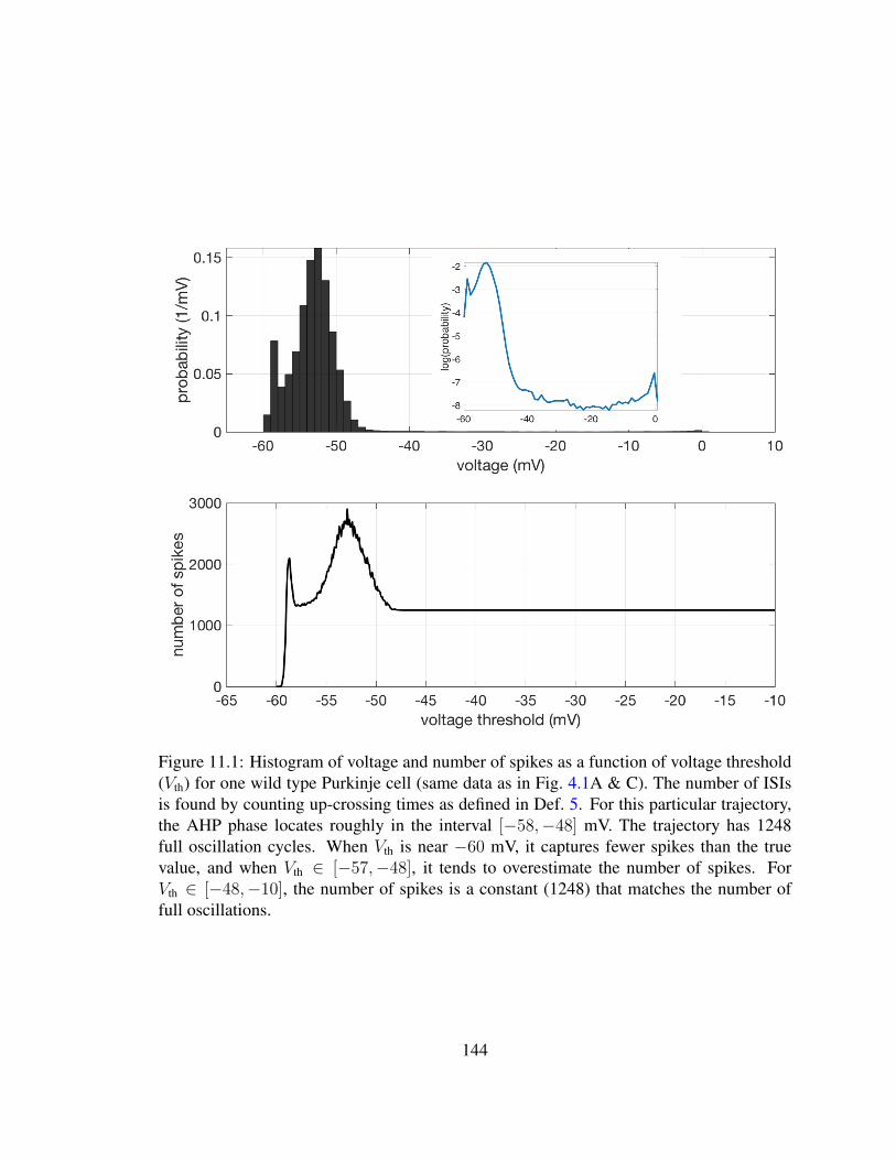
Figure 11.1: Histogram of voltage and number of spikes as a function of voltage threshold(Vth) for one wild type Purkinje cell (same data as in Fig. 4.1A & C). The number of ISIsis found by counting up-crossing times as defined in Def. 5. For this particular trajectory,the AHP phase locates roughly in the interval [−58,−48] mV. The trajectory has 1248full oscillation cycles. When Vth is near −60 mV, it captures fewer spikes than the truevalue, and when Vth ∈ [−57,−48], it tends to overestimate the number of spikes. ForVth ∈ [−48,−10], the number of spikes is a constant (1248) that matches the number offull oscillations.
144
threshold or trigger level was immaterial, provided it was high enough to avoid background
noise and low enough to capture every action potential [44, 84]. This assumption is
generally left implicit. Here, we show that, in fact, the choice of the trigger level (the
voltage threshold used for identifying spike timing) can cause a change in the variance of
the interspike interval for a given spike train by as much as 5%.
Fig. 11.2 provides evidence both from experimental traces recorded in vitro, and from
numerical simulations, that σ2ISI is sensitive to the voltage threshold defining spike times.
In Fig. 11.2 A, we superimpose ISI standard deviations from fourteen wild type Purkinje
cells, plotted as functions of the the trigger voltage Vth. We rescale each plot by the standard
deviation of the ISI for each cell at Vth = −20 mV, which we define as σ. As shown in
Fig. 11.2 A, the cells recorded in vitro have a clear variability in the standard deviation
as the voltage threshold changes. Specifically, the standard deviation of ISI gradually
increases as voltage threshold increases and then remains constant as the threshold ap-
proaches the peak of the spikes. Two of the cells have larger variations in the standard
deviation, with roughly a 3%−4% change; nine of them have a 1%−3% change; and three
of them show 0.1%− 1% change.
We applied a similar analysis to seventeen PCs with leaner mutations. In this case, one
cell had a variation of roughly 1% in the standard deviation, five cells with variations around
0.2%, and the remaining without an obvious change (data not shown). This difference
between cells derived from wild type and leaner mutant mice is an interesting topic for
future study.
We observe a similar variability of σ2ISI in numerical simulations using our stochastic
Langevin HH model (cf. eqn. (9.28)). Fig. 11.2 B and C plots two examples showing
the change in σ2ISI as voltage threshold varies. For a given noise level (ε) and a voltage
threshold (Vth), a single run simulates a total time of 9000 milliseconds (ms), with a time
145
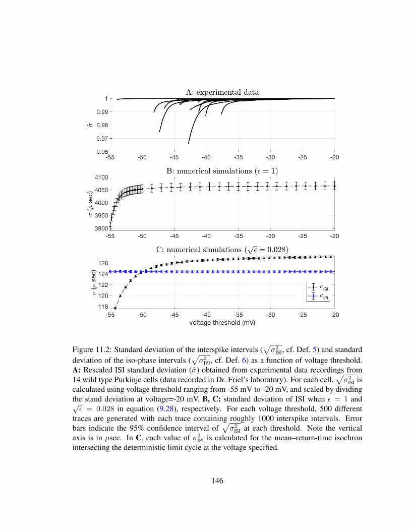
Figure 11.2: Standard deviation of the interspike intervals (√σ2
ISI, cf. Def. 5) and standarddeviation of the iso-phase intervals (
√σ2
IPI, cf. Def. 6) as a function of voltage threshold.A: Rescaled ISI standard deviation (σ) obtained from experimental data recordings from14 wild type Purkinje cells (data recorded in Dr. Friel’s laboratory). For each cell,
√σ2
ISI iscalculated using voltage threshold ranging from -55 mV to -20 mV, and scaled by dividingthe stand deviation at voltage=-20 mV. B, C: standard deviation of ISI when ε = 1 and√ε = 0.028 in equation (9.28), respectively. For each voltage threshold, 500 different
traces are generated with each trace containing roughly 1000 interspike intervals. Errorbars indicate the 95% confidence interval of
√σ2
ISI at each threshold. Note the verticalaxis is in µsec. In C, each value of σ2
IPI is calculated for the mean–return-time isochronintersecting the deterministic limit cycle at the voltage specified.
146
step of 0.008 ms, consisting of at least 600 ISIs, which was collected as one realization
for the corresponding σISI(ε, Vth). The mean and standard deviation of the σISI(ε, Vth) is
calculated for 1,000 realizations of the aforementioned step for each pair of ε and Vth. The
error bars in Fig. 11.2 B and C indicate 95% confidence intervals of the standard deviation.
As illustrated in Fig. 11.2 B and C, the standard deviation gradually increases as the trigger
threshold increases during the AHP, and this trend is observed for both small and large
noises. When ε = 1, the noisy system in eqn. (9.28) is not close to the deterministic
limit cycle, and there is not a good approximation for the phase response curve. When√ε = 0.028, the system eqn. (9.28) can be considered in the small-noise region and thus
we can find a corresponding phase on the limit cycle as the asymptotic phase. As shown
in Fig. 11.2 C, unlike the variance of ISI, the variance of IPI is invariant with the choice of
the phase threshold (φ).
11.2 Numerical Performance of the Decomposition Theo-
rem
In this section, we will apply estimation methods based on Theorem 4 and Corollary 7 to
the decomposition of variance of interspike intervals (ISIs, σ2ISI) and variance of inter-phase
intervals (IPIs, σ2IPI), and numerically test their performance.
Fig. 11.3 presents a detailed comparison of the predicted and measured values of σ2ISI
and σ2IPI, when the simulations only include noise from the K+ channels. The channel noise
generated by the Na+ edges is suppressed by applying the stochastic shielding (SS) method
to eqn. (9.28). For each plot in Fig. 11.3, 1000 repeated trials are collected and each trial
simulates a total time of 15,000 milliseconds which generates more than 1000 ISIs or IPIs.
Given our previous observation that σ2ISI depends on the choice of voltage threshold, we
147
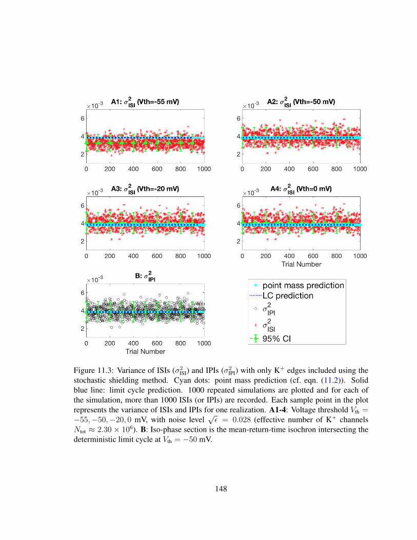
Figure 11.3: Variance of ISIs (σ2ISI) and IPIs (σ2
IPI) with only K+ edges included using thestochastic shielding method. Cyan dots: point mass prediction (cf. eqn. (11.2)). Solidblue line: limit cycle prediction. 1000 repeated simulations are plotted and for each ofthe simulation, more than 1000 ISIs (or IPIs) are recorded. Each sample point in the plotrepresents the variance of ISIs and IPIs for one realization. A1-4: Voltage threshold Vth =−55,−50,−20, 0 mV, with noise level
√ε = 0.028 (effective number of K+ channels
Ntot ≈ 2.30× 10⁶). B: Iso-phase section is the mean-return-time isochron intersecting thedeterministic limit cycle at Vth = −50 mV.
148
selected four different voltage thresholds for comparison.
In Fig. 11.3, red dots in panels A1-A4 mark the ISI variance measured directly from
simulated voltage traces, using the indicated Vth as the trigger voltage. Green stem-and-
line marks show the mean and 95% confidence intervals of the direct ISI variance measure,
calculated from all 1000 samples. The blue dotted line shows the ISI variance predicted
from the limit cycle based estimate of the IPI variance (eq. (10.58)), and cyan squares show
individual estimates using the point-mass prediction (eq. (11.3)). Note each point mass
is an independent random variable; these estimates cluster tightly around the limit cycle
based estimate. Panel B shows the variance of the inter-phase intervals calculated directly
from the same 1000 trajectories (as described below), marked in black circles. Green stem-
and-line marks show the mean and 95% C.I. for the IPI variance. The blue dotted line and
cyan squares represent the same LC-based and point mass based IPI variance estimates as
in A1-A4.
As shown in Fig. 11.3 (A1, A2, A3, A4 and B) the point mass prediction and the LC
prediction of the IPI variance give almost the same result. Specifically, the LC prediction≈
3.84×10⁻³ and the mean of the point mass predictions≈ 3.83×10⁻³ with a variance of≈
6.3×10⁻¹¹. Therefore, the LC prediction based on Corollary 7 gives a good approximation
to the point mass prediction based directly on Theorem 4. For a given edge (or a group
of edges) the LC prediction depends linearly on the scaling factor, ε, and can be easily
calculated for various noise levels. Throughout the rest of this section, we will use the LC
prediction as our predicted contribution from the decomposition theorem.
The asymptotic phase is calculated using equation (11.2) for each point on the stochastic
trajectory. For a given voltage threshold, Vth, the corresponding iso-phase section is the
mean-return-time isochron intersecting the deterministic limit cycle at Vth. As previously
observed, the variance of the IPIs is invariant with respect to the choice of the reference iso-
149
phase section. As shown in Fig. 11.3 B, the prediction of variance of IPIs (≈ 3.83 × 10⁻³
ms2) has a good match with the mean value of numerical simulations (≈ 3.85 × 10⁻³
ms2). The 95% confidence interval of the IPIs are also plotted in Fig. 11.3 B, which further
indicates the reliability of the prediction.
As shown in Fig. 11.3 (A1, A2, A3 and A4), with Vth ∈ [−55, 0] mV, the numerical re-
alizations of σ2ISI are close to the predictions from the main theorem. However, the accuracy
depends on the choice of the voltage threshold. As noted above, when the trigger voltage
Vth is set below −50mV (for example, −55mV in Fig. 11.3,A1), the measured variance
of ISIs falls below the value predicted from the IPI variance. When Vth ≈ −50mV, the
empirically observed value of σ2ISI gives the best match to the IPI variance (cf. Fig. 11.2,C).
When the trigger voltage Vth exceeds −50mV (for example, −20mV in Fig. 11.3,A3, and
0mV in Fig. 11.3,A4), the empirically observed variance of the ISIs is consistently higher
than the IPI variance. Nevertheless, although the empirically observed numerical values
of σ2ISI (≈ 4.00 × 10⁻³ms2) overestimate the IPI-derived value when Vth > −50mV, they
remain close to the IPI value. Fig. 11.3 panels A1-4 show that even though the IPI-based
prediction of the ISI variance works best when the trigger voltage is set to Vth ≈ −50mV,
the IPI-based variance falls within the 95% confidence interval of σ2ISI regardless of the
value of Vth chosen. Therefore, we can conclude that Theorem 4 and Corollary 7 give a
good approximation to the value of σ2ISI, at least at noise level
√ε = 0.028.
Practically, the voltage-based interspike interval variance, σ2ISI, is a more widely used
quantity [57, 74, 86, 112, 118] because it can be calculated directly from electrophysio-
logical recordings. The inter-phase interval variance, σ2IPI, however, can not be directly
measured or calculated. Even given the stochastic model with its realizations, calculating
the asymptotic phase and finding the IPIs are numerically expensive. Despite its lack of
consistency, as shown in Fig. 11.3 (A3 and A4), the σ2ISI can approximately be decom-
150
posed using Theorem 4 and Corollary 7, which offer predicted values that fall in the 95%
confidence interval of σ2ISI.
Fig. 11.4 summarizes the overall fit of the decomposition of variance of ISIs to the
prediction from Theorem 4 and Corollary 7. We applied the stochastic shielding method
by including each directed edge separately in the transition graph (cf. Fig. 3.1). In Fig. 11.4
(B and D), the variance of the ISIs is compared with the value obtained with the limit cycle
based prediction from eqn. (10.58).
Fig. 11.4 (A and C) shows the log-log plot for the ISI variance (σ2ISI) of each individual
edge as a function of the noise level, ε, in the range of [e−10, e5], measured via direct
numerical simulation using Vth = −20 mV. The color for each edge ranges from red to blue
according an ascending order of edge numbers (1-8 for K+ and 1-20 for Na+). The total
effective number of Na+ channels is Mtot = Mref/ε and of K+ channels is Ntot = Nref/ε,
where the reference channel numbers are Mref = 6000 and Nref = 1800 (described in §9.4).
That is, we consider ranges of channel numbers 40 . Mtot . 1.3 × 10⁸ for Na+ and
12 . Ntot . 4.0 × 10⁷ for K+. Thus, we cover the entire range of empirically observed
single-cell channel populations (cf. Tab. 3.1).
As shown in Fig. 11.4 (A and C), the linear relation between σ2ISI and ε predicted from
Theorem 4 is numerically observed for all 28 directed edges in the Na+ and K+ transition
graphs (cf. 3.1) for small noise. The same rank order of edge importance discussed in §6.5
is also observed here in the small noise region. Moreover, the smaller the edge importance
measure for an individual edge, the larger the value of ε before observing a breakdown of
linearity.
Fig. 11.4 (B and D) presents the log-log plot for the ISI variance (σ2ISI, black solid line)
when including noise only from the K+ edges and Na+ edges, respectively. As in panels
A and C, the noise level, ε is in the range of [e−10, e5]. The LC prediction for eqn. (10.58)
151
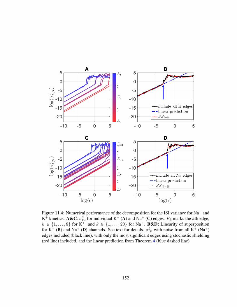
Figure 11.4: Numerical performance of the decomposition for the ISI variance for Na+ andK+ kinetics. A&C: σ2
ISI for individual K+ (A) and Na+ (C) edges. Ek marks the kth edge,k ∈ 1, . . . , 8 for K+ and k ∈ 1, . . . , 20 for Na+. B&D: Linearity of superpositionfor K+ (B) and Na+ (D) channels. See text for details. σ2
ISI with noise from all K+ (Na+)edges included (black line), with only the most significant edges using stochastic shielding(red line) included, and the linear prediction from Theorem 4 (blue dashed line).
152
from Theorem 4 when including noise from only the K+ (or Na+) channels is plotted in
dashed blue. For example, the linear noise prediction for the potassium channels alone is
σ2ISI ≈
EK∑k=1
σ2ISI,k (11.4)
where EK = 8 (similarly, ENa = 20), and σ2ISI,k is the LC prediction for the kth edge.
As shown in Fig. 11.4 panel B, the linear prediction matches well with the numerically
calculated σ2ISI up to ln(ε) ≈ −3.0 (indicated by the blue arrow) which corresponds to
approximately 36,000 K+ channels. For Na+, the theorem gives a good prediction of the
numerical σ2ISI up to ln(ε) ≈ −1.9 (indicated by the blue arrow) which corresponds to
approximately 40,000 Na+ channels. These channel population sizes are consistent with
typical single-cell ion channel populations, such as the population of Na+ channels in the
node of Ranvier, or the Na+ and K+ channels in models of the soma of a cerebellar Purkinje
cell (cf. Tab. 3.1).
Finally, we apply stochastic shielding (SS) to both the K+and Na+channels by only
including noise from the edges making the largest contributions in Fig. 11.4 panels A and
C. For the K+ channel, we include edges 7 and 8, and for Na+, we include edges 17, 18,
19 and 20. As shown in Fig. 11.4 panels B and D, the SS method (solid red line) gives
a good match to the overall σ2ISI for all noise intensities ε ∈ [e−10, e5], with numbers of
K+ channels ≥ 12 and Na+ channels ≥ 40.
Fig. 11.5 shows the overall performance of the prediction of σ2ISI based on Theorem 4,
when noise from all 28 directed edges are included (black line). The theorem is stated as an
asymptotic result in the limit of weak noise. The predicted ISI variance using the theorem
(dashed blue curve) matches the ISI variance obtained from the full numerical simulation
for modest noise levels, up to ln(ε) ≤ −3.9, corresponding to & 90,000 K+ channels and
153
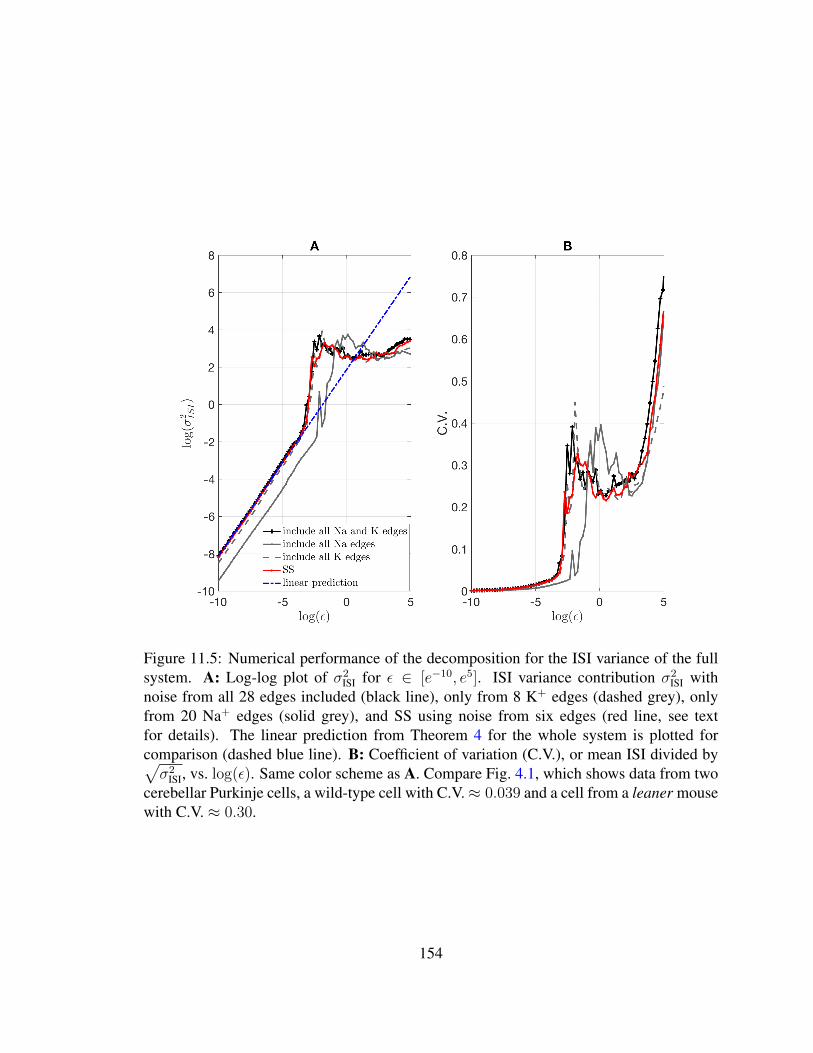
Figure 11.5: Numerical performance of the decomposition for the ISI variance of the fullsystem. A: Log-log plot of σ2
ISI for ε ∈ [e−10, e5]. ISI variance contribution σ2ISI with
noise from all 28 edges included (black line), only from 8 K+ edges (dashed grey), onlyfrom 20 Na+ edges (solid grey), and SS using noise from six edges (red line, see textfor details). The linear prediction from Theorem 4 for the whole system is plotted forcomparison (dashed blue line). B: Coefficient of variation (C.V.), or mean ISI divided by√σ2
ISI, vs. log(ε). Same color scheme as A. Compare Fig. 4.1, which shows data from twocerebellar Purkinje cells, a wild-type cell with C.V.≈ 0.039 and a cell from a leaner mousewith C.V. ≈ 0.30.
154
& 300,000 Na+ channels. These population sizes are at the high end of the range of typical
numbers of channels neurons (cf. Tab. 3.1).
For smaller ion channel populations (larger noise levels), the linear approximation
breaks down, but the stochastic shielding approximation remains in good agreement with
full numerical simulations. Fig. 11.5 shows σ2ISI from simulations using the SS method
including only noise from the six most important edges (edges 7-8 in K+ and 17-20 in
Na+), plotted in solid red. For ln(ε) & −3.5, both the full simulation and the SS simulation
show a rapid increase in σ2ISI with increasing noise level. This dramatic increase in timing
variability results when increasing noise causes the neuron to “miss” spikes, that is, to
generate a mixture of regular spiking and small subthreshold oscillations [101]. Including
noise from all 20 Na+ channel edges (gray line) or all eight K+ channel edges (gray dashed
line) shows a similar jump, albeit delayed to higher values of ε for the Na+ channel. Note
also the Na+ channel alone has a quantitatively smaller contribution to ISI variability for
the stochastic HH model than the K+ channel for all noise levels in the linear region.
For larger noise levels (ln(ε) & −2), all simulations become sufficiently noisy that
ln(σ2ISI) collapse to a similar level, approximately 3. As the interspike interval is a non-
negative random quantity with a constrained mean (bounded by the reciprocal of the firing
rate), once the spike train has maximal variability, further increasing the strength of the
channel noise does not drive the ISI variance appreciably higher. However, although the
ISI variance appears approximately to saturate with increasing noise, the coefficient of
variation (C.V.,√σ2
ISI/I) continues to increase (Fig. 11.5B), because the mean ISI (I)
decreases with increasing noise (the firing rate increases with increasing noise, data not
shown).
155
Part V
Conclusions and Discussion
156
Chapter 12
Conclusions
12.1 Summary
The exact method for Markov chain (MC) simulation for an electrotonically compact (sin-
gle compartment) conductance-based stochastic model under current clamp is a hybrid
discrete (channel state) / continuous (voltage) model of the sort used by [4, 18, 87]. While
MC methods are computationally expensive, simulations based on Gaussian/Langevin ap-
proximations can capture the effects of stochastic ion channel fluctuations with reason-
able accuracy and excellent computational efficiency. Since Goldwyn and Shea Brown’s
work focusing the attention of the computational neuroscience community on Fox and
Lu’s Langevin algorithm for the Hodgkin-Huxley system [39, 49], several variants of this
approach have appeared in the literature.
In this thesis, as in [95], we advocate for a class of models combining the best features
of conductance-based Langevin models with the recently developed stochastic shielding
approximation [102, 104, 105]. We propose a Langevin model with a 14-dimensional
157
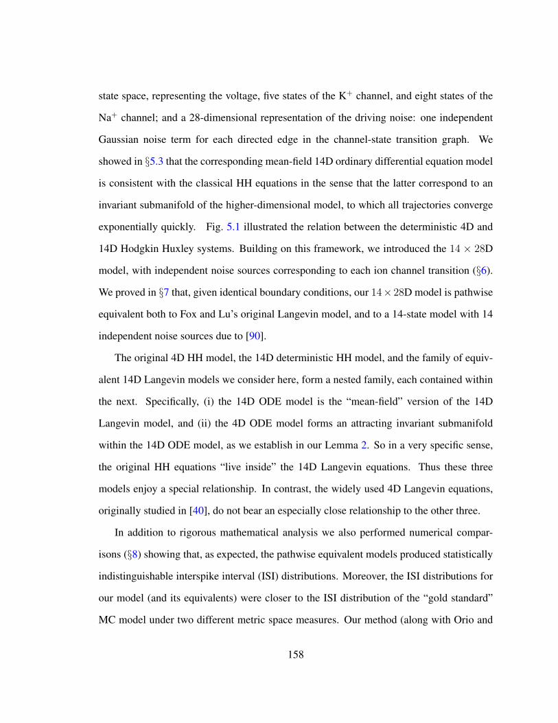
state space, representing the voltage, five states of the K+ channel, and eight states of the
Na+ channel; and a 28-dimensional representation of the driving noise: one independent
Gaussian noise term for each directed edge in the channel-state transition graph. We
showed in §5.3 that the corresponding mean-field 14D ordinary differential equation model
is consistent with the classical HH equations in the sense that the latter correspond to an
invariant submanifold of the higher-dimensional model, to which all trajectories converge
exponentially quickly. Fig. 5.1 illustrated the relation between the deterministic 4D and
14D Hodgkin Huxley systems. Building on this framework, we introduced the 14 × 28D
model, with independent noise sources corresponding to each ion channel transition (§6).
We proved in §7 that, given identical boundary conditions, our 14×28D model is pathwise
equivalent both to Fox and Lu’s original Langevin model, and to a 14-state model with 14
independent noise sources due to [90].
The original 4D HH model, the 14D deterministic HH model, and the family of equiv-
alent 14D Langevin models we consider here, form a nested family, each contained within
the next. Specifically, (i) the 14D ODE model is the “mean-field” version of the 14D
Langevin model, and (ii) the 4D ODE model forms an attracting invariant submanifold
within the 14D ODE model, as we establish in our Lemma 2. So in a very specific sense,
the original HH equations “live inside” the 14D Langevin equations. Thus these three
models enjoy a special relationship. In contrast, the widely used 4D Langevin equations,
originally studied in [40], do not bear an especially close relationship to the other three.
In addition to rigorous mathematical analysis we also performed numerical compar-
isons (§8) showing that, as expected, the pathwise equivalent models produced statistically
indistinguishable interspike interval (ISI) distributions. Moreover, the ISI distributions for
our model (and its equivalents) were closer to the ISI distribution of the “gold standard”
MC model under two different metric space measures. Our method (along with Orio and
158
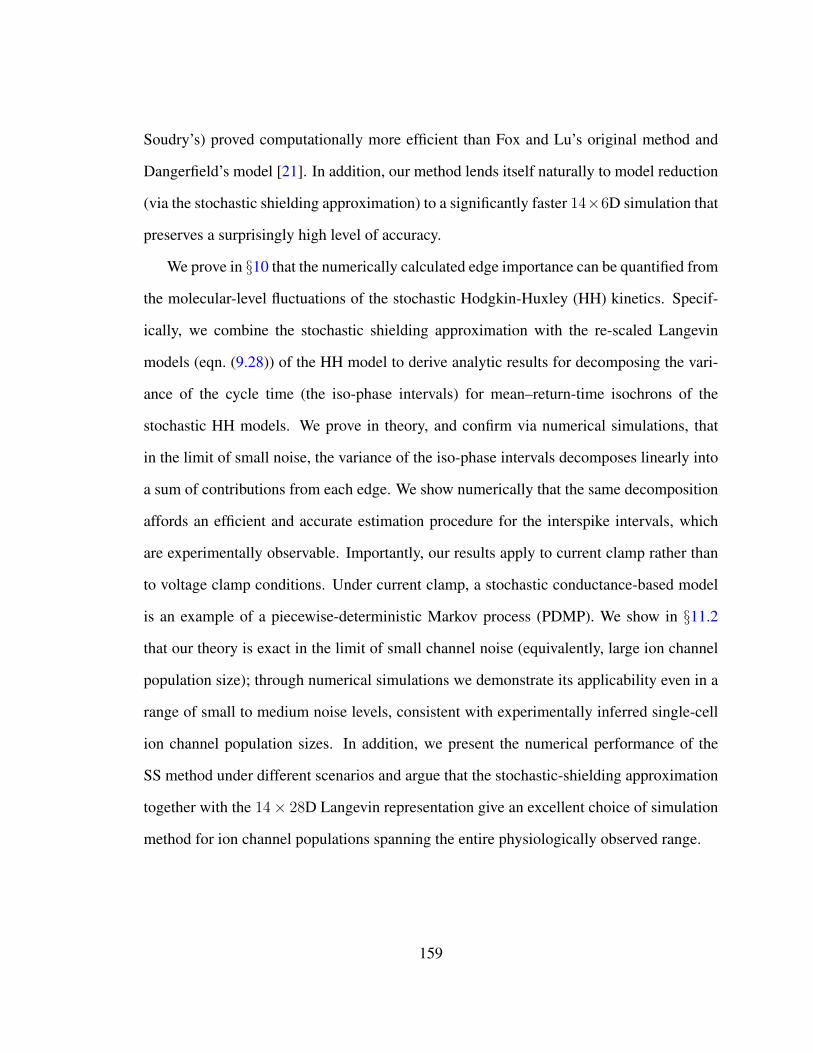
Soudry’s) proved computationally more efficient than Fox and Lu’s original method and
Dangerfield’s model [21]. In addition, our method lends itself naturally to model reduction
(via the stochastic shielding approximation) to a significantly faster 14×6D simulation that
preserves a surprisingly high level of accuracy.
We prove in §10 that the numerically calculated edge importance can be quantified from
the molecular-level fluctuations of the stochastic Hodgkin-Huxley (HH) kinetics. Specif-
ically, we combine the stochastic shielding approximation with the re-scaled Langevin
models (eqn. (9.28)) of the HH model to derive analytic results for decomposing the vari-
ance of the cycle time (the iso-phase intervals) for mean–return-time isochrons of the
stochastic HH models. We prove in theory, and confirm via numerical simulations, that
in the limit of small noise, the variance of the iso-phase intervals decomposes linearly into
a sum of contributions from each edge. We show numerically that the same decomposition
affords an efficient and accurate estimation procedure for the interspike intervals, which
are experimentally observable. Importantly, our results apply to current clamp rather than
to voltage clamp conditions. Under current clamp, a stochastic conductance-based model
is an example of a piecewise-deterministic Markov process (PDMP). We show in §11.2
that our theory is exact in the limit of small channel noise (equivalently, large ion channel
population size); through numerical simulations we demonstrate its applicability even in a
range of small to medium noise levels, consistent with experimentally inferred single-cell
ion channel population sizes. In addition, we present the numerical performance of the
SS method under different scenarios and argue that the stochastic-shielding approximation
together with the 14× 28D Langevin representation give an excellent choice of simulation
method for ion channel populations spanning the entire physiologically observed range.
159
Chapter 13
Discussions
13.1 Discrete Gillespie Markov Chain Algorithms
The discrete-state Markov chain algorithm due to Gillespie is often taken to be the gold
standard simulation for a single-compartment stochastic conductance-based model. Most
former literature on Langevin HH models, such as [49, 60, 73, 90], when establishing a
reference MC model, consider a version of the discrete Gillespie algorithm that assumes
a piecewise-constant propensity approximation, i.e. that does not take into account that
the voltage changes between transitions, which changes the transition rates. This approx-
imation can lead to biophysically unrealistic voltage traces for very small system sizes
(cf. Fig. 2 of [67], top trace with N = 1 ion channel) although the differences appear to be
mitigated for N & 40 channels [4]. In the present thesis, our MC simulations are based on
6000 Na+ and 1800 K+ channels (as in [49]), and we too use the ISI distribution generated
by a piecewise-constant propensity MC algorithm as our reference distribution. Given the
range of physiologically observed single-cell ion channel population sizes (Tab. 3.1), it ap-
160
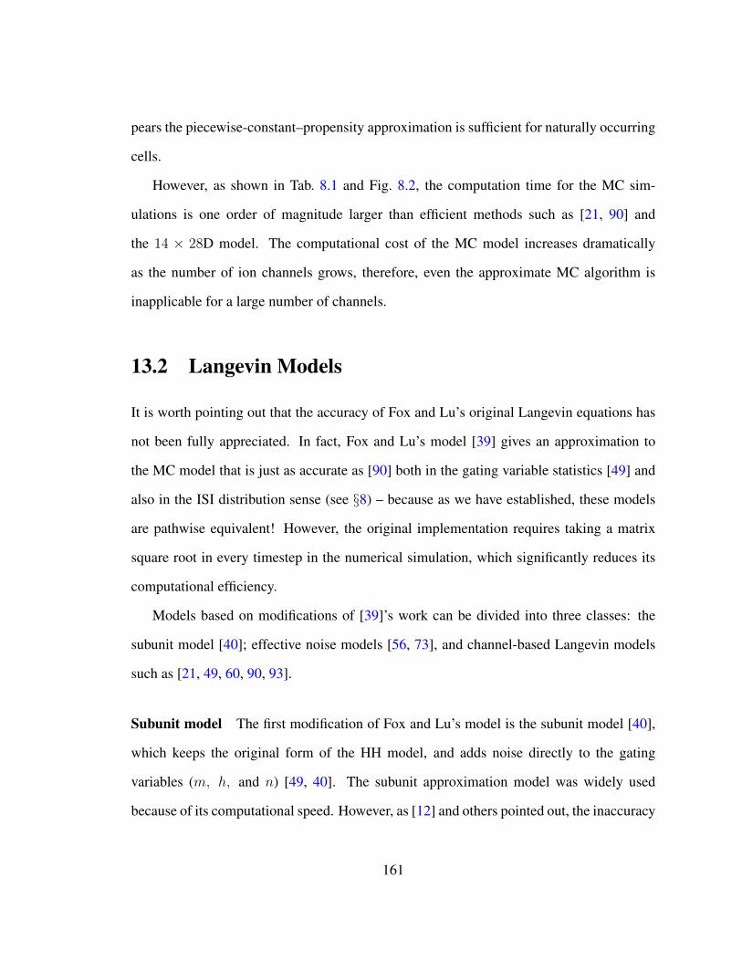
pears the piecewise-constant–propensity approximation is sufficient for naturally occurring
cells.
However, as shown in Tab. 8.1 and Fig. 8.2, the computation time for the MC sim-
ulations is one order of magnitude larger than efficient methods such as [21, 90] and
the 14 × 28D model. The computational cost of the MC model increases dramatically
as the number of ion channels grows, therefore, even the approximate MC algorithm is
inapplicable for a large number of channels.
13.2 Langevin Models
It is worth pointing out that the accuracy of Fox and Lu’s original Langevin equations has
not been fully appreciated. In fact, Fox and Lu’s model [39] gives an approximation to
the MC model that is just as accurate as [90] both in the gating variable statistics [49] and
also in the ISI distribution sense (see §8) – because as we have established, these models
are pathwise equivalent! However, the original implementation requires taking a matrix
square root in every timestep in the numerical simulation, which significantly reduces its
computational efficiency.
Models based on modifications of [39]’s work can be divided into three classes: the
subunit model [40]; effective noise models [56, 73], and channel-based Langevin models
such as [21, 49, 60, 90, 93].
Subunit model The first modification of Fox and Lu’s model is the subunit model [40],
which keeps the original form of the HH model, and adds noise directly to the gating
variables (m, h, and n) [49, 40]. The subunit approximation model was widely used
because of its computational speed. However, as [12] and others pointed out, the inaccuracy
161
of this model remains significant even for large number of channels. Moreover, [49] and
[61] found that the subunit model fails to capture the statistics of the HH Na+ and K+ gates.
In this thesis, we also observed that the subunit model is more efficient than channel-based
Langevin models, but tends to delay spike generation. As shown in Fig. 8.1, the subunit
model generates significantly longer ISIs than the MC model.
Effective noise models Another modification to Fox and Lu’s algorithm is to add colored
noise to the channel open fractions. We did not include colored noise models such as [73,
56] in our model comparison. However, [61] found that both these effective noise models
generate shorter ISIs than the MC model with the same parameters. Though the comparison
we provided in §8 only include the Fox and Lu 94, Fox97, Goldwyn, Dangerfield, Orio, SS
and the 14 × 28D model, combining the results from [49] and [61], the 14 × 28D model
could be compared to a variety of models including [21, 39, 40, 49, 56, 60, 73, 90].
Channel-based Langevin models The main focus of Part III (§7-§8) of this thesis is the
modification based on the original Fox and Lu’s matrix decomposition method, namely, the
channel-based (or conductance-based) Langevin models. We proved in §7 that under the
same boundary conditions, Fox and Lu’s original model, Orio’s model and our 14 × 28D
model are pathwise equivalent, which was also verified from our numerical simulations
in §7 and §8. In §7, we discussed channel-based Langevin models including [21, 39,
41, 49, 90]. We excluded Fox’s more recent implementation [41] in §8 for two reasons.
First, the algorithm is pathwise equivalent to others considered there. And moreover, the
method is vulnerable to numerical instability when performing the Cholesky decomposi-
tion. Specifically, some of the elements in the S matrix from the Cholesky decomposition
in [41] involve square roots of differences of several quantities, with no guarantee that the
162
differences will result in nonnegative terms – even with strictly positive values of the gating
variables. Nevertheless, this model would be in the equivalence class and in any case would
not be more efficient than Orio’s model, because of the noise dimension and complicated
operations (e.g. taking multiple square roots) in each time step.
13.3 Model Comparisons
If two random variables have similar distributions, then they will have similar moments,
but not necessarily vice-versa. Therefore, comparison of the full interspike-interval dis-
tributions produced by different simulation algorithms gives a more rigorous test than
comparison of first and second moments of the ISI distribution. Most previous evaluations
of competing Langevin approximations were based on the accuracy of low-order moments,
for example the mean and variance of channel state occupancy under voltage clamp, or the
mean and variance of the interspike interval distribution under current clamp [21, 48, 49,
60, 61, 73, 90, 102]. In this thesis, we compare the accuracy of the different algorithms
using the full ISI distribution, but using the L1 norm of the difference (Wasserstein metric)
and the L∞ norm (Kolmogorov-Smirnov test). The paper [52] previously compared the ISI
distributions generated by the Markov chain (Gillespie algorithm) to the distribution gener-
ated by different types of Langevin approximations (LA), including the original Langevin
models [39, 49], the channel-based LA with colored noise [56, 73], and LA with a 14× 14
variant of the diffusion coefficient matrix S [90]. They concluded that Orio and Soudry’s
method provided the best match to the Markov chain model, specifically “Fox-Goldwyn,
and Orio-Kurtz1 methods both generate ISI histograms very close to those of Micro2” [52].
We note that the comparison reported in this paper simply superimposed plots of the ISI
1We refer to this model as to as “Orio”2This is the model we refer to as the Markov-chain model.
163
distributions, allowing a qualitative comparison, while our metric-space analysis is fully
quantitative. In any case, their conclusions are consistent with our findings; we showed
in §7 that the Fox-Goldwyn and the Orio-Kurtz model are pathwise equivalent (when
implemented with the same boundary conditions), which accounts for the similarity in the
ISI histograms they generate. In fact, because of pathwise equivalence, we can conclude
that the true distributions for these models are identical, and any differences observed just
reflect finite sampling.
13.4 Stochastic Shielding Method
The stochastic shielding (SS) approximation [102] provides an efficient and accurate method
for approximating a Markov process using only a subset of transitions to generate fluctu-
ations, namely those directly involving observable states. For conductance-based models,
rather than aggregating ion channel states, SS effects dimension reduction by selectively
eliminating those independent noise sources (channel state transitions) that have the least
impact on current fluctuations. Recent work in [93] compared previous methods such as
[21, 46, 60, 90, 102] in accuracy, applicability and simplicity as well as computational
efficiency. They concluded that for mesoscopic numbers of channels, stochastic shielding
methods combined with diffusion approximation methods can be an optimal choice. That
is precisely the combination of methods that we advocate in this thesis.
Like [90], the stochastic shielding method proposed by [93] assumed detailed balance
of transitions between adjacent states and used edges that are directly connected to the open
gates of HH Na+ and K+. We calculated the edge importance in §6.5 and found that the
four (out of twenty) most important directed edges for the Na+ gates are not the four edges
directly connected to the conducting state, as assumed in previous application of the SS
164
method [102], but rather the two pairs of edges “upstream” of the open state, which are the
transitions typically leading to initiation of a voltage spike.
13.5 Which Model to Use?
Among all the modifications of Fox and Lu’s method considered here, Orio and Soudry’s
approach, and our 14× 28D model, provide the best approximation to the “gold standard”
MC model, with the greatest computational efficiency. Several earlier models were studied
in the review paper by [49], where they rediscovered that the original Langevin model pro-
posed by Fox and Lu is the best approximation to the MC model among those considered.
Later work ([61]) further surveyed a wide range of Langevin approximations for the HH
system including [39, 40, 49, 56, 60, 73, 90] and explored models with different boundary
conditions. The survey [61] concluded that the bounded and truncated-restored Langevin
model [60] and the unbounded [90]’s model provide the best approximation to the MC
model.
As shown in §7 and §8, the 14 × 28D Langevin model naturally derived from the
channel structure is pathwise equivalent to the Fox and Lu ‘94, Fox ‘18, and the Orio-
Soudry models under the same boundary conditions. The 14 × 28D model (with open
boundary conditions) is more accurate than models with the reflecting boundary condition
method of [21], and also better than the approximation method proposed by [49], when
the entire ISI distribution is taken into account. We note that [61, 111] treated Goldwyn’s
method [49] as the original Fox and Lu model in their comparison, however, the simulation
in [49] uses the 4D multinomial submanifold to update the gating variables. Our analysis
and numerical simulations suggest that the original Fox and Lu model is indeed as accurate
as the Orio-Soudry model, while the computational cost still remains a major concern.
165
Though the 14×28D model has similar efficiency and accuracy with [90], it has several
advantages. First, the rectangular S matrix (in eqn. (3.2)-(3.3)) in Orio’s model merges
the noise contributions of reciprocal pairs of edges. However, this dimension reduction
assumes, in effect, that detailed balance holds along reciprocal edges, which our results
show is not the case, under current clamp (Fig. 6.2). Moreover, the 14 × 28D model
arises naturally from the individual transitions of the exact evolution equations (eqn.(6.14)-
(6.15)) for the underlying Markov chain model, which makes it conceptually easier to
understand. In addition, our method for defining the 14 × 28D Langevin model and
finding the best SS model extends to channel-based models with arbitrary channel gating
schemes beyond the standard HH model. Given any channel state transition graph, the
Langevin equations may be read off from the transitions, and the edge importance under
current clamp can be evaluated by applying the stochastic shielding method to investigate
the contributions of noise from each individual directed edge. Finally, in exchange for
a small reduction in accuracy, the stochastic shielding method affords a significant gain in
efficiency. The 14×28D model thus offers a natural way to quantify the contributions of the
microscopic transitions to the macroscopic voltage fluctuations in the membrane through
the use of stochastic shielding. For general ion channel models, extending a biophysically-
based Langevin model analogous to our 14× 28D HH model, together with the stochastic
shielding method, may provide the best available tool for investigating how unobservable
microscopic behaviors (such as ion channel fluctuations) affect the macroscopic variability
in many biological systems.
166
13.6 Variance of Interspike Intervals
There are several different methods for detecting spikes and quantifying interspike intervals
(ISIs). In one widely used approach [44, 57, 74, 84, 86, 112, 118], we can define the
threshold as the time of upcrossing a fixed voltage, which is also called a Schmitt trigger
(after O.H. Schmitt [106]). We primarily use this method in this thesis.
As an alternative, the time at which the rate of change of voltage, dV/dt, reaches its
maximum value (within a given spike) has also been used as the condition for detecting
spikes [7]. However, in contrast with the voltage-based Schmitt trigger, using the maximum
of dV/dt to localize the spike does not give a well-defined Poincare section. To see this,
consider that for a system of the form (7.6) we would have to set
d2V
dt2=
d
dtf(V,N) (13.1)
= f(V,N)∂f
∂V(V,N)− dM8
dtgNa(V − VNa)−
dN5
dtgK(V − VK)
equal to zero to find the corresponding section. The difficulty is evident: for the Langevin
system the open fraction M8 (resp. N5) of sodium (resp. potassium) channels is a diffusion
process, and is not differentiable, so “dM8/dt” and “dN5/dt” are not well defined. More-
over, even if we could interpret these expressions, the set of voltages V and gating variables
N for which (13.1) equals zero depends on the instantaneous value of the noise forcing,
so the corresponding section would not be fixed within the phase space. For a discrete
state stochastic channel model, the point of maximum rate of change of voltage could be
determined post-hoc from a trajectory, but again depends on the random waiting times
between events, and so is not a fixed set of points in phase space. For these reasons we do
not further analyze ISIs based on this method of defining spikes, although we nevertheless
167
include numerical ISI variance based on this method, for comparison (see Fig. 13.1 below).
As a third possibility, used for example in [57], one sets the voltage nullcline (dV/dt =
0), at the top of the spike, as the Poincare section for spike detection. That is, one uses
a surface such as Speak = (v,n) | f(v,n) = 0 ∩ v > −40. This condition does
correspond to a well-defined Poincare section, albeit one with a different normal direction
than the voltage-based sections.
In contrast to the ISI variance, which depends to some degree on the choice of spike-
timing method used, the mean ISI is invariant. Both in numerical simulations and from
experimental recordings, the mean interspike interval using any of the three methods above
is very stable. But the apparent ISI variance changes, depending on the method chosen.
We observe in both real and simulated voltage traces that the ISI variance, σ2ISI, depends
not only on the method for identifying spikes, but also on the voltage used for the Schmitt
trigger. To our knowledge this sensitivity of ISI variance to trigger voltage has not been
previously reported. Generally speaking, from analyzing both simulation and recorded
data from in vitro studies, the ISI variance is not a constant, but increases slightly as the
voltage threshold defining a “spike” is increased (cf. §11.1). Thus the ISI variance is not an
intrinsically precisely invariant quantity for model or real nerve cells.
Fig. 13.1 shows σ2ISI obtained empirically from electrophysiological recordings of Purk-
inje cells in vitro (upper plot) and from simulations of the stochastic Hodgkin-Huxley
system (lower plot) with a small noise amplitude (√ε = 0.028) using the three methods for
spike time extraction described above, for a single voltage trace comprising 785 interspike
intervals. The ISI variance as a function of trigger voltage increases steadily from below
7.8 ms2 to above 7.9 ms2 as the trigger voltage increases from -50 mV to -20 mV. In
contrast, the ISI variance obtained from the peak voltage (dV/dt ≈ 0, obtained using
linear interpolation of the first-order voltage difference) or the maximum slope condition
168
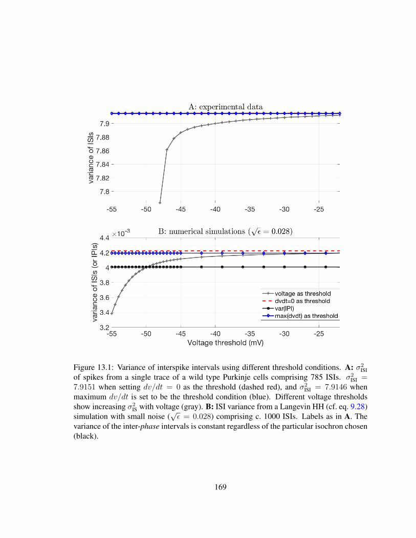
Figure 13.1: Variance of interspike intervals using different threshold conditions. A: σ2ISI
of spikes from a single trace of a wild type Purkinje cells comprising 785 ISIs. σ2ISI =
7.9151 when setting dv/dt = 0 as the threshold (dashed red), and σ2ISI = 7.9146 when
maximum dv/dt is set to be the threshold condition (blue). Different voltage thresholdsshow increasing σ2
IS with voltage (gray). B: ISI variance from a Langevin HH (cf. eq. 9.28)simulation with small noise (
√ε = 0.028) comprising c. 1000 ISIs. Labels as in A. The
variance of the inter-phase intervals is constant regardless of the particular isochron chosen(black).
169
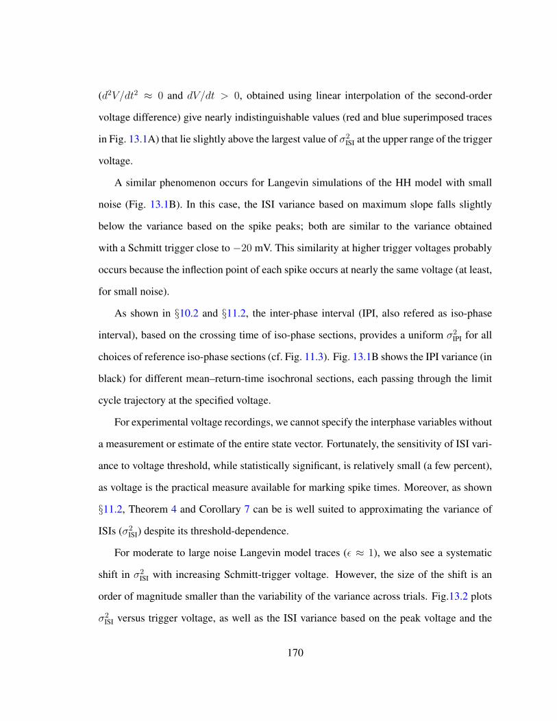
(d2V/dt2 ≈ 0 and dV/dt > 0, obtained using linear interpolation of the second-order
voltage difference) give nearly indistinguishable values (red and blue superimposed traces
in Fig. 13.1A) that lie slightly above the largest value of σ2ISI at the upper range of the trigger
voltage.
A similar phenomenon occurs for Langevin simulations of the HH model with small
noise (Fig. 13.1B). In this case, the ISI variance based on maximum slope falls slightly
below the variance based on the spike peaks; both are similar to the variance obtained
with a Schmitt trigger close to −20 mV. This similarity at higher trigger voltages probably
occurs because the inflection point of each spike occurs at nearly the same voltage (at least,
for small noise).
As shown in §10.2 and §11.2, the inter-phase interval (IPI, also refered as iso-phase
interval), based on the crossing time of iso-phase sections, provides a uniform σ2IPI for all
choices of reference iso-phase sections (cf. Fig. 11.3). Fig. 13.1B shows the IPI variance (in
black) for different mean–return-time isochronal sections, each passing through the limit
cycle trajectory at the specified voltage.
For experimental voltage recordings, we cannot specify the interphase variables without
a measurement or estimate of the entire state vector. Fortunately, the sensitivity of ISI vari-
ance to voltage threshold, while statistically significant, is relatively small (a few percent),
as voltage is the practical measure available for marking spike times. Moreover, as shown
§11.2, Theorem 4 and Corollary 7 can be is well suited to approximating the variance of
ISIs (σ2ISI) despite its threshold-dependence.
For moderate to large noise Langevin model traces (ε ≈ 1), we also see a systematic
shift in σ2ISI with increasing Schmitt-trigger voltage. However, the size of the shift is an
order of magnitude smaller than the variability of the variance across trials. Fig.13.2 plots
σ2ISI versus trigger voltage, as well as the ISI variance based on the peak voltage and the
170
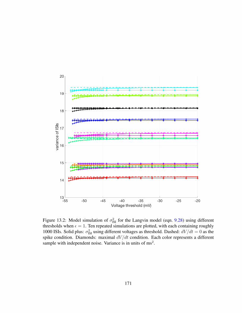
Figure 13.2: Model simulation of σ2ISI for the Langvin model (eqn. 9.28) using different
thresholds when ε = 1. Ten repeated simulations are plotted, with each containing roughly1000 ISIs. Solid plus: σ2
ISI using different voltages as threshold. Dashed: dV/dt = 0 as thespike condition. Diamonds: maximal dV/dt condition. Each color represents a differentsample with independent noise. Variance is in units of ms2.
171
maximal slope conditions, for ten different samples of the Langevin HH model with ε = 1,
each comprising & 1000 interspike intervals. In each case σ2ISI is a smoothly increasing
function of the trigger voltage, but the range of the increase in variance is approximately
0.25 ms2, while the sample variance of the ISI variance itself is approximately 3.5 ms2
across the ten trials, an order of magnitude larger. For comparison, the sample variance of
σ2ISI across c. 4000 trials, cf. Fig. 11.3, is approximately 3 × 10⁻⁷ ms2. The source of the
variance for the larger noise value may involve the introduction of extra or missing spikes
from the regular spiking pattern, cf. Fig. 11.5. Thus, although σ2ISI based on the standard
Schmitt trigger approach is sensitive to the trigger value, the IPI variance estimate given by
Theorem 4 lies within the range of this sensitivity, which for realistic noise levels is small
compared to the intrinsic variability of the variance across trials.
172
Chapter 14
Limitations
All Langevin models, including our proposed 14× 28D model, proceed from the assump-
tion that the ion channel population is large enough (and the ion channel state transitions
frequent enough) that the Gaussian approximations by which the white noise forcing terms
are derived, are justified. Thus when the system size is too small, no Langevin system
will be an appropriate. Fortunately the Langevin approximation appears quite accurate for
realistic population sizes (cf. Tab. 3.1 and Figs. 11.4-11.5).
The 14×28D model uses more noise sources than other approaches. However, stochas-
tic shielding allows us to jettison noise sources that do not significantly impact the system
dynamics (the voltage fluctuations and ISI distribution). Moreover, in order to compare
the ISI distribution in detail among several variants of the Fox and Lu ’94 model versus
the Markov chain standard, we have considered a single value of the driving current, while
other studies have compared parametrized responses such as the firing rate, ISI variance,
or other moments, as a function of applied current. Accurate comparisons require large
ensembles of independent trajectories, forcing a tradeoff between precision and breadth;
173
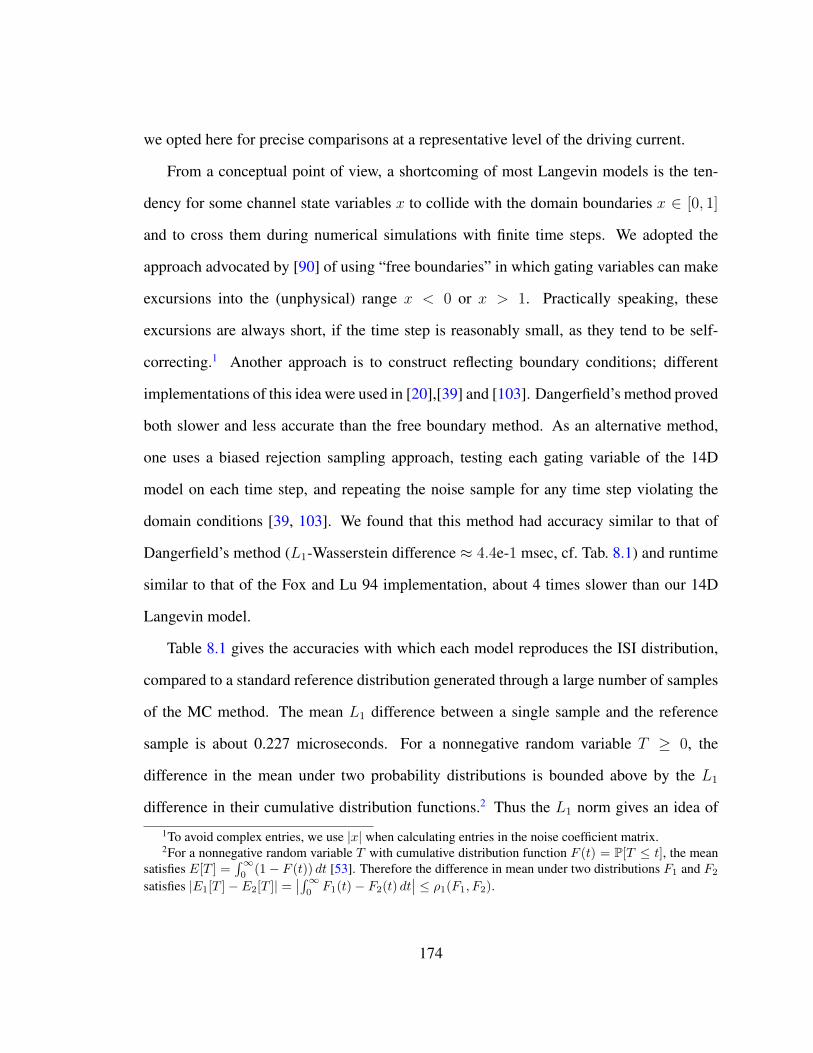
we opted here for precise comparisons at a representative level of the driving current.
From a conceptual point of view, a shortcoming of most Langevin models is the ten-
dency for some channel state variables x to collide with the domain boundaries x ∈ [0, 1]
and to cross them during numerical simulations with finite time steps. We adopted the
approach advocated by [90] of using “free boundaries” in which gating variables can make
excursions into the (unphysical) range x < 0 or x > 1. Practically speaking, these
excursions are always short, if the time step is reasonably small, as they tend to be self-
correcting.1 Another approach is to construct reflecting boundary conditions; different
implementations of this idea were used in [20],[39] and [103]. Dangerfield’s method proved
both slower and less accurate than the free boundary method. As an alternative method,
one uses a biased rejection sampling approach, testing each gating variable of the 14D
model on each time step, and repeating the noise sample for any time step violating the
domain conditions [39, 103]. We found that this method had accuracy similar to that of
Dangerfield’s method (L1-Wasserstein difference ≈ 4.4e-1 msec, cf. Tab. 8.1) and runtime
similar to that of the Fox and Lu 94 implementation, about 4 times slower than our 14D
Langevin model.
Table 8.1 gives the accuracies with which each model reproduces the ISI distribution,
compared to a standard reference distribution generated through a large number of samples
of the MC method. The mean L1 difference between a single sample and the reference
sample is about 0.227 microseconds. For a nonnegative random variable T ≥ 0, the
difference in the mean under two probability distributions is bounded above by the L1
difference in their cumulative distribution functions.2 Thus the L1 norm gives an idea of
1To avoid complex entries, we use |x| when calculating entries in the noise coefficient matrix.2For a nonnegative random variable T with cumulative distribution function F (t) = P[T ≤ t], the mean
satisfies E[T ] =∫∞0
(1− F (t)) dt [53]. Therefore the difference in mean under two distributions F1 and F2
satisfies |E1[T ]− E2[T ]| =∣∣∫∞
0F1(t)− F2(t) dt
∣∣ ≤ ρ1(F1, F2).
174
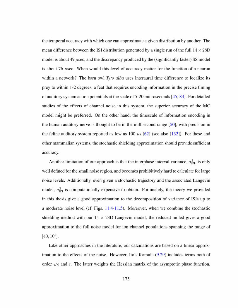
the temporal accuracy with which one can approximate a given distribution by another. The
mean difference between the ISI distribution generated by a single run of the full 14× 28D
model is about 49 µsec, and the discrepancy produced by the (significantly faster) SS model
is about 76 µsec. When would this level of accuracy matter for the function of a neuron
within a network? The barn owl Tyto alba uses interaural time difference to localize its
prey to within 1-2 degrees, a feat that requires encoding information in the precise timing
of auditory system action potentials at the scale of 5-20 microseconds [45, 83]. For detailed
studies of the effects of channel noise in this system, the superior accuracy of the MC
model might be preferred. On the other hand, the timescale of information encoding in
the human auditory nerve is thought to be in the millisecond range [50], with precision in
the feline auditory system reported as low as 100 µs [62] (see also [132]). For these and
other mammalian systems, the stochastic shielding approximation should provide sufficient
accuracy.
Another limitation of our approach is that the interphase interval variance, σ2IPI, is only
well defined for the small noise region, and becomes prohibitively hard to calculate for large
noise levels. Additionally, even given a stochastic trajectory and the associated Langevin
model, σ2IPI is computationally expensive to obtain. Fortunately, the theory we provided
in this thesis give a good approximation to the decomposition of variance of ISIs up to
a moderate noise level (cf. Figs. 11.4-11.5). Moreover, when we combine the stochastic
shielding method with our 14 × 28D Langevin model, the reduced moled gives a good
approximation to the full noise model for ion channel populations spanning the range of
[40, 105].
Like other approaches in the literature, our calculations are based on a linear approx-
imation to the effects of the noise. However, Ito’s formula (9.29) includes terms both of
order√ε and ε. The latter weights the Hessian matrix of the asymptotic phase function,
175
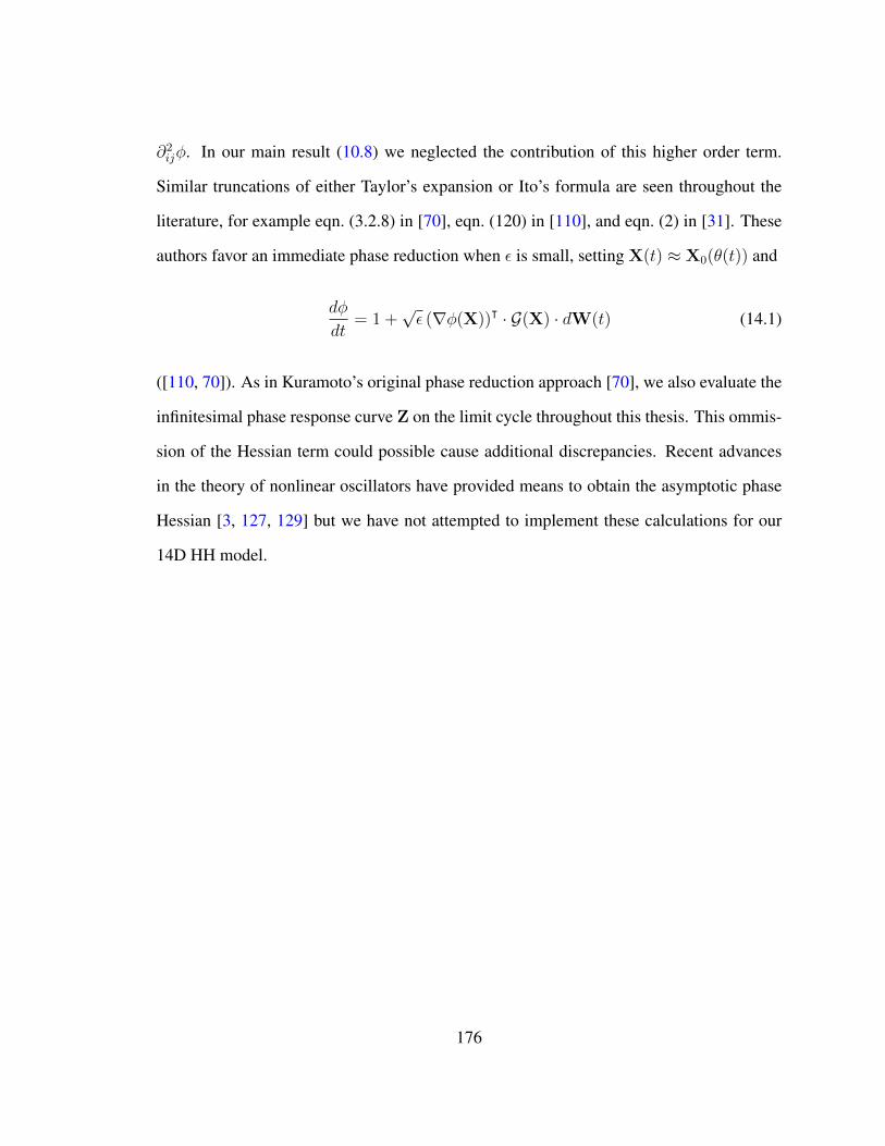
∂2ijφ. In our main result (10.8) we neglected the contribution of this higher order term.
Similar truncations of either Taylor’s expansion or Ito’s formula are seen throughout the
literature, for example eqn. (3.2.8) in [70], eqn. (120) in [110], and eqn. (2) in [31]. These
authors favor an immediate phase reduction when ε is small, setting X(t) ≈ X0(θ(t)) and
dφ
dt= 1 +
√ε (∇φ(X))ᵀ · G(X) · dW(t) (14.1)
([110, 70]). As in Kuramoto’s original phase reduction approach [70], we also evaluate the
infinitesimal phase response curve Z on the limit cycle throughout this thesis. This ommis-
sion of the Hessian term could possible cause additional discrepancies. Recent advances
in the theory of nonlinear oscillators have provided means to obtain the asymptotic phase
Hessian [3, 127, 129] but we have not attempted to implement these calculations for our
14D HH model.
176

Appendix A
Table of Common Symbols and
Notations
Symbol MeaningC Membrane capacitance (µF/cm2)v Membrane potential (mV )VNa, VK, VL Ionic reversal potential for Na+, K+and leak (mV )gion maximal conductance for ion ∈ Na+,K+Iapp Applied current to the membrane (nA/cm2)m, h, n Dimensionless gating variables for Na+ and K+ channelsαx, βx , x ∈ m,n, h Voltage dependent rate constant (1/msec)x vector of state variablesM = [M1,M2, · · · ,M8] Eight-component state vector for the Na+ gates[m00, · · · ,m30,m01, · · · ,m31]
ᵀ Components for the Na+gatesN = [N1,N2, · · · ,N5] Five-component state vector for the K+ gates[n0, n1, n2, n3, n4]
ᵀ Components for the K+ gatesMtot, Ntot Total number of Na+ and K+ channels
Table A.1: Common symbols and notations in this thesis (part I).
177
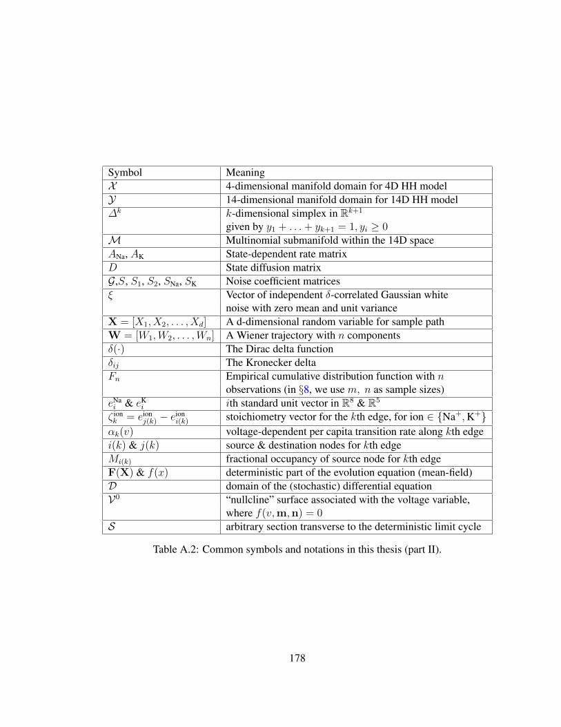
Symbol MeaningX 4-dimensional manifold domain for 4D HH modelY 14-dimensional manifold domain for 14D HH model∆k k-dimensional simplex in Rk+1
given by y1 + . . .+ yk+1 = 1, yi ≥ 0M Multinomial submanifold within the 14D spaceANa, AK State-dependent rate matrixD State diffusion matrixG,S, S1, S2, SNa, SK Noise coefficient matricesξ Vector of independent δ-correlated Gaussian white
noise with zero mean and unit varianceX = [X1, X2, . . . , Xd] A d-dimensional random variable for sample pathW = [W1,W2, . . . ,Wn] A Wiener trajectory with n componentsδ(·) The Dirac delta functionδij The Kronecker deltaFn Empirical cumulative distribution function with n
observations (in §8, we use m, n as sample sizes)eNai & eK
i ith standard unit vector in R8 & R5
ζ ionk = eion
j(k) − eioni(k) stoichiometry vector for the kth edge, for ion ∈ Na+,K+
αk(v) voltage-dependent per capita transition rate along kth edgei(k) & j(k) source & destination nodes for kth edgeMi(k) fractional occupancy of source node for kth edgeF(X) & f(x) deterministic part of the evolution equation (mean-field)D domain of the (stochastic) differential equationV0 “nullcline” surface associated with the voltage variable,
where f(v,m,n) = 0S arbitrary section transverse to the deterministic limit cycle
Table A.2: Common symbols and notations in this thesis (part II).
178
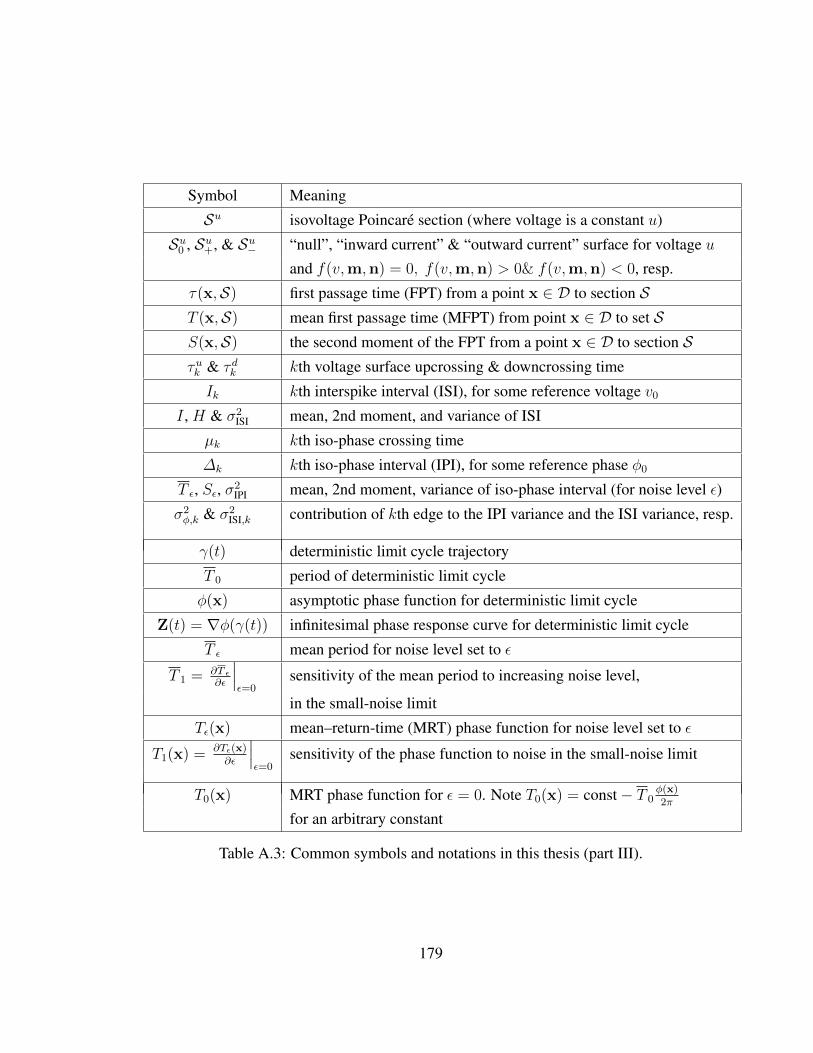
Symbol Meaning
Su isovoltage Poincare section (where voltage is a constant u)
Su0 , Su+, & Su− “null”, “inward current” & “outward current” surface for voltage u
and f(v,m,n) = 0, f(v,m,n) > 0& f(v,m,n) < 0, resp.
τ(x,S) first passage time (FPT) from a point x ∈ D to section ST (x,S) mean first passage time (MFPT) from point x ∈ D to set SS(x,S) the second moment of the FPT from a point x ∈ D to section Sτuk & τ dk kth voltage surface upcrossing & downcrossing time
Ik kth interspike interval (ISI), for some reference voltage v0I , H & σ2
ISI mean, 2nd moment, and variance of ISI
µk kth iso-phase crossing time
∆k kth iso-phase interval (IPI), for some reference phase φ0
T ε, Sε, σ2IPI mean, 2nd moment, variance of iso-phase interval (for noise level ε)
σ2φ,k & σ2
ISI,k contribution of kth edge to the IPI variance and the ISI variance, resp.
γ(t) deterministic limit cycle trajectory
T 0 period of deterministic limit cycle
φ(x) asymptotic phase function for deterministic limit cycle
Z(t) = ∇φ(γ(t)) infinitesimal phase response curve for deterministic limit cycle
T ε mean period for noise level set to ε
T 1 = ∂T ε∂ε
∣∣∣ε=0
sensitivity of the mean period to increasing noise level,
in the small-noise limit
Tε(x) mean–return-time (MRT) phase function for noise level set to ε
T1(x) = ∂Tε(x)∂ε
∣∣∣ε=0
sensitivity of the phase function to noise in the small-noise limit
T0(x) MRT phase function for ε = 0. Note T0(x) = const− T 0φ(x)2π
for an arbitrary constant
Table A.3: Common symbols and notations in this thesis (part III).
179
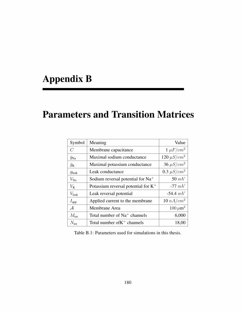
Appendix B
Parameters and Transition Matrices
Symbol Meaning Value
C Membrane capacitance 1 µF/cm2
gNa Maximal sodium conductance 120 µS/cm2
gK Maximal potassium conductance 36 µS/cm2
gleak Leak conductance 0.3 µS/cm2
VNa Sodium reversal potential for Na+ 50 mV
VK Potassium reversal potential for K+ -77 mV
Vleak Leak reversal potential -54.4 mV
Iapp Applied current to the membrane 10 nA/cm2
A Membrane Area 100µm2
Mtot Total number of Na+ channels 6,000
Ntot Total number ofK+ channels 18,00
Table B.1: Parameters used for simulations in this thesis.
180
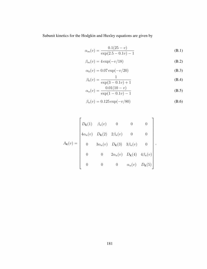
Subunit kinetics for the Hodgkin and Huxley equations are given by
αm(v) =0.1(25− v)
exp(2.5− 0.1v)− 1(B.1)
βm(v) = 4 exp(−v/18) (B.2)
αh(v) = 0.07 exp(−v/20) (B.3)
βh(v) =1
exp(3− 0.1v) + 1(B.4)
αn(v) =0.01(10− v)
exp(1− 0.1v)− 1(B.5)
βn(v) = 0.125 exp(−v/80) (B.6)
AK(v) =
DK(1) βn(v) 0 0 0
4αn(v) DK(2) 2βn(v) 0 0
0 3αn(v) DK(3) 3βn(v) 0
0 0 2αn(v) DK(4) 4βn(v)
0 0 0 αn(v) DK(5)
,
181
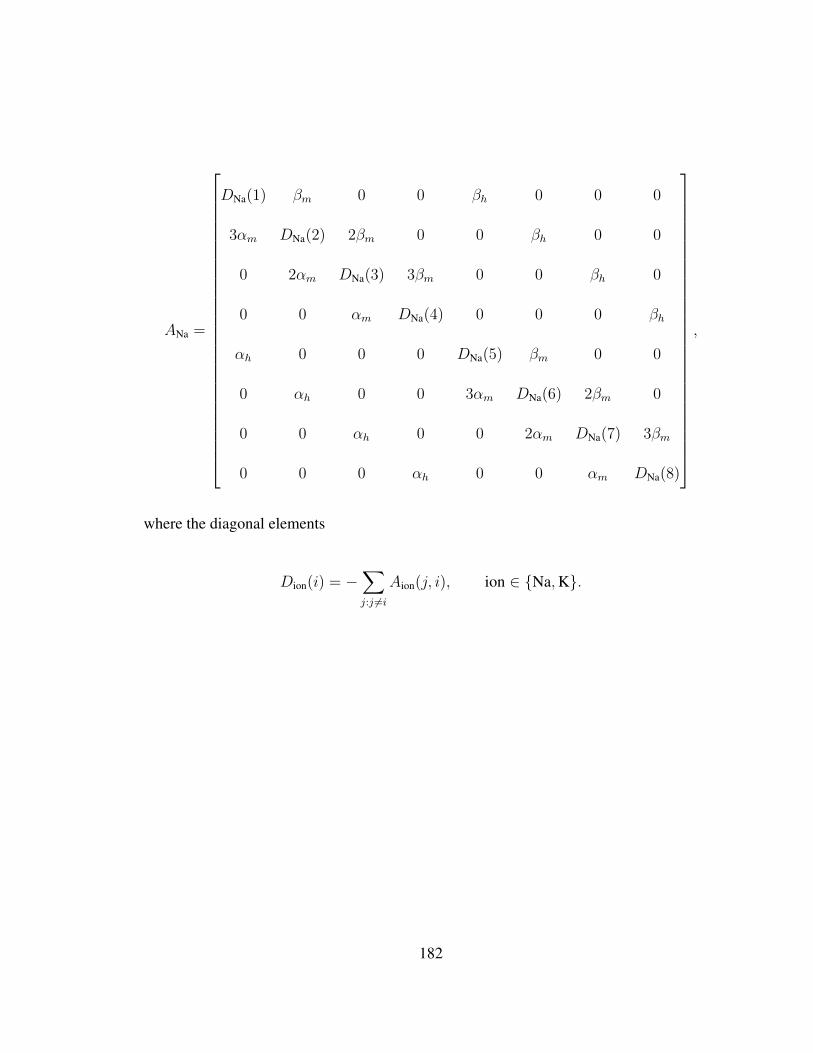
ANa =
DNa(1) βm 0 0 βh 0 0 0
3αm DNa(2) 2βm 0 0 βh 0 0
0 2αm DNa(3) 3βm 0 0 βh 0
0 0 αm DNa(4) 0 0 0 βh
αh 0 0 0 DNa(5) βm 0 0
0 αh 0 0 3αm DNa(6) 2βm 0
0 0 αh 0 0 2αm DNa(7) 3βm
0 0 0 αh 0 0 αm DNa(8)
,
where the diagonal elements
Dion(i) = −∑j:j 6=i
Aion(j, i), ion ∈ Na,K.
182
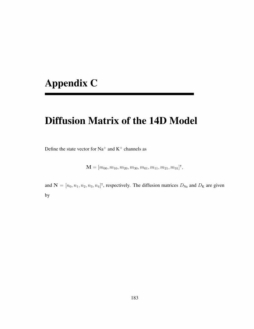
Appendix C
Diffusion Matrix of the 14D Model
Define the state vector for Na+ and K+ channels as
M = [m00,m10,m20,m30,m01,m11,m21,m31]ᵀ,
and N = [n0, n1, n2, n3, n4]ᵀ, respectively. The diffusion matrices DNa and DK are given
by
183
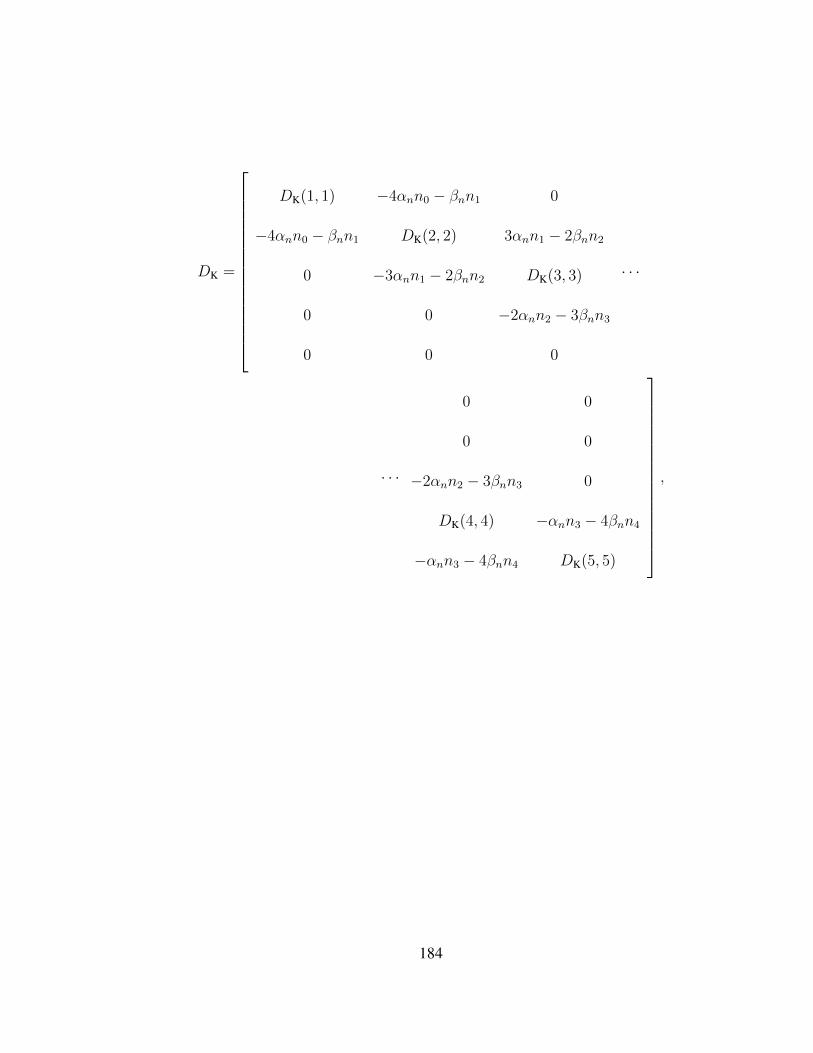
DK =
DK(1, 1) −4αnn0 − βnn1 0
−4αnn0 − βnn1 DK(2, 2) 3αnn1 − 2βnn2
0 −3αnn1 − 2βnn2 DK(3, 3)
0 0 −2αnn2 − 3βnn3
0 0 0
· · ·
· · ·
0 0
0 0
−2αnn2 − 3βnn3 0
DK(4, 4) −αnn3 − 4βnn4
−αnn3 − 4βnn4 DK(5, 5)
,
184
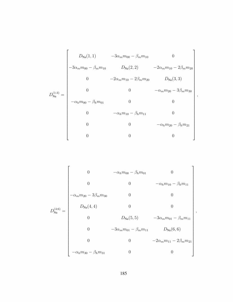
D(1:3)Na =
DNa(1, 1) −3αmm00 − βmm10 0
−3αmm00 − βmm10 DNa(2, 2) −2αmm10 − 2βmm20
0 −2αmm10 − 2βmm20 DNa(3, 3)
0 0 −αmm20 − 3βmm30
−αhm00 − βhm01 0 0
0 −αhm10 − βhm11 0
0 0 −αhm20 − βhm21
0 0 0
,
D(4:6)Na =
0 −αhm00 − βhm01 0
0 0 −αhm10 − βhm11
−αmm20 − 3βmm30 0 0
DNa(4, 4) 0 0
0 DNa(5, 5) −3αmm01 − βmm11
0 −3αmm01 − βmm11 DNa(6, 6)
0 0 −2αmm11 − 2βmm21
−αhm30 − βhm31 0 0
,
185
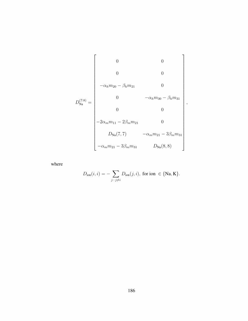
D(7:8)Na =
0 0
0 0
−αhm20 − βhm21 0
0 −αhm30 − βhm31
0 0
−2αmm11 − 2βmm21 0
DNa(7, 7) −αmm21 − 3βmm31
−αmm21 − 3βmm31 DNa(8, 8)
,
where
Dion(i, i) = −∑j : j 6=i
Dion(j, i), for ion ∈ Na,K.
186

Bibliography[1] L.F Abbott. Lapicque’s introduction of the integrate-and-fire model neuron (1907).
Brain Research Bulletin, 50(5–6):303 – 304, 1999.
[2] Edward J Allen, Linda JS Allen, Armando Arciniega, and Priscilla E Greenwood.Construction of equivalent stochastic differential equation models. StochasticAnalysis and Applications, 26(2):274–297, 2008.
[3] Z. Aminzare, P. Holmes, and V. Srivastava. On phase reduction and time period ofnoisy oscillators. In 2019 IEEE 58th Conference on Decision and Control (CDC),pages 4717–4722, 2019.
[4] David F. Anderson, Bard Ermentrout, and Peter J. Thomas. Stochasticrepresentations of ion channel kinetics and exact stochastic simulation of neuronaldynamics. Journal of Computational Neuroscience, 38(1):67–82, 2015.
[5] David F. Anderson, Arnab Ganguly, and Thomas G. Kurtz. Error analysis of tau-leapsimulation methods. Ann. Appl. Probab., 21(6):2226–2262, December 2011.
[6] David F Anderson and Thomas G Kurtz. Stochastic Analysis of BiochemicalSystems, volume 1. Springer, 2015.
[7] Rony Azouz and Charles M Gray. Dynamic spike threshold reveals a mechanismfor synaptic coincidence detection in cortical neurons in vivo. Proceedings of theNational Academy of Sciences, 97(14):8110–8115, 2000.
[8] Mark W Barnett and Philip M Larkman. The action potential. Practical Neurology,7(3):192–197, 2007.
[9] Francisco Bezanilla. Single sodium channels from the squid giant axon. BiophysicalJournal, 52(6):1087–1090, 1987.
[10] Paul C Bressloff and Jay M Newby. Path integrals and large deviations in stochastichybrid systems. Physical Review E, 89(4):042701, 2014.
[11] Eric Brown, Jeff Moehlis, and Philip Holmes. On the phase reduction and responsedynamics of neural oscillator populations. Neural Comput, 16(4):673–715, Apr2004.
[12] Ian C Bruce. Evaluation of stochastic differential equation approximation of ionchannel gating models. Annals of Biomedical Engineering, 37(4):824–838, 2009.
[13] Nicolas Brunel and Peter E Latham. Firing rate of the noisy quadratic integrate-and-fire neuron. Neural Computation, 15(10):2281–2306, 2003.
187
[14] Evelyn Buckwar and Martin G Riedler. An exact stochastic hybrid model ofexcitable membranes including spatio-temporal evolution. Journal of MathematicalBiology, 63(6):1051–1093, 2011.
[15] Robert J Butera Jr, John Rinzel, and Jeffrey C Smith. Models of respiratory rhythmgeneration in the pre-botzinger complex. i. bursting pacemaker neurons. Journal ofNeurophysiology, 82(1):382–397, 1999.
[16] Daniela Calvetti and Erkki Somersalo. Introduction to Bayesian ScientificComputing: Ten Lectures on Subjective Computing. Springer, 2007.
[17] Brett C Carter, Andrew J Giessel, Bernardo L Sabatini, and Bruce P Bean. Transientsodium current at subthreshold voltages: activation by epsp waveforms. Neuron,75(6):1081–93, Sep 2012.
[18] J R Clay and L J DeFelice. Relationship between membrane excitability and singlechannel open-close kinetics. Biophys J, 42(2):151–7, May 1983.
[19] David Colquhoun and AG Hawkes. On the stochastic properties of single ionchannels. Proc. R. Soc. Lond. B, 211(1183):205–235, 1981.
[20] CE Dangerfield, David Kay, and Kevin Burrage. Stochastic models and simulationof ion channel dynamics. Procedia Computer Science, 1(1):1587–1596, 2010.
[21] Ciara E Dangerfield, David Kay, and Kevin Burrage. Modeling ion channeldynamics through reflected stochastic differential equations. Physical Review E,85(5):051907, 2012.
[22] Peter Dayan and L. F. Abbott. Theoretical neuroscience: computational andmathematical modeling of neural systems. Computational Neuroscience. The MITPress, 2001.
[23] Erik De Schutter and James M Bower. An active membrane model of the cerebellarPurkinje cell I. Simulation of current clamps in slice. Journal of neurophysiology,71(1):375–400, 1994.
[24] Erik De Schutter and James M Bower. An active membrane model of the cerebellarPurkinje cell II. Simulation of synaptic responses. Journal of Neurophysiology,71(1):401–419, 1994.
[25] Erik De Schutter and James M Bower. Simulated responses of cerebellar Purkinjecells are independent of the dendritic location of granule cell synaptic inputs.Proceedings of the National Academy of Sciences, 91(11):4736–4740, 1994.
188
[26] Alan D Dorval and John A White. Channel noise is essential for perithresholdoscillations in entorhinal stellate neurons. Journal of neuroscience, 25(43):10025–10028, 2005.
[27] JE Dowling. An introduction to neuroscience, 1992.
[28] Aryeh Dvoretzky, Jack Kiefer, and Jacob Wolfowitz. Asymptotic minimax characterof the sample distribution function and of the classical multinomial estimator. TheAnnals of Mathematical Statistics, 27(3):642–669, 1956.
[29] B. Earnshaw and J. Keener. Global asymptotic stability of solutions ofnonautonomous master equations. SIAM Journal on Applied Dynamical Systems,9(1):220–237, 2010.
[30] B. Earnshaw and J. Keener. Invariant manifolds of binomial-like nonautonomousmaster equations. SIAM Journal on Applied Dynamical Systems, 9(2):568–588,2010.
[31] G Bard Ermentrout, Bryce Beverlin, 2nd, Todd Troyer, and Theoden I Netoff. Thevariance of phase-resetting curves. J Comput Neurosci, Jan 2011.
[32] G. Bard Ermentrout and David H. Terman. Foundations Of MathematicalNeuroscience. Springer, 2010.
[33] A Aldo Faisal and Simon B Laughlin. Stochastic simulations on the reliability ofaction potential propagation in thin axons. PLoS Computational Biology, 3(5), 2007.
[34] A Aldo Faisal, John A White, and Simon B Laughlin. Ion-channel noise placeslimits on the miniaturization of the brain’s wiring. Current Biology, 15(12):1143–1149, 2005.
[35] Elizabeth M Fenwick, A Marty, and E Neher. Sodium and calcium channels inbovine chromaffin cells. The Journal of physiology, 331(1):599–635, 1982.
[36] Fernando R Fernandez, Jordan D T Engbers, and Ray W Turner. Firing dynamics ofcerebellar Purkinje cells. J Neurophysiol, 98(1):278–94, Jul 2007.
[37] Michael D Forrest. Intracellular calcium dynamics permit a purkinje neuron modelto perform toggle and gain computations upon its inputs. Frontiers in computationalneuroscience, 8:86, 2014.
[38] Michael D Forrest. Simulation of alcohol action upon a detailed Purkinjeneuron model and a simpler surrogate model that runs>400 times faster. BMCNeuroscience, 16(1):27, 2015.
189
[39] Fox and Lu. Emergent collective behavior in large numbers of globally coupledindependently stochastic ion channels. Phys Rev E Stat Phys Plasmas Fluids RelatInterdiscip Topics, 49(4):3421–3431, Apr 1994.
[40] Ronald F Fox. Stochastic versions of the Hodgkin-Huxley equations. BiophysicalJournal, 72(5):2068–2074, 1997.
[41] Ronald F Fox. Critique of the Fox-Lu model for Hodgkin-Huxley fluctuations inneuron ion channels. arXiv preprint arXiv:1807.07632, 2018.
[42] Chetan Gadgil, Chang Hyeong Lee, and Hans G. Othmer. A stochastic analysis offirst-order reaction networks. Bulletin of Mathematical Biology, 67, 2005.
[43] Crispin W. Gardiner. Handbook of Stochastic Methods for Physics, Chemistry, andthe Natural Sciences. Springer Verlag, 2nd edition, 2004.
[44] George L Gerstein. Analysis of firing patterns in single neurons. Science,131(3416):1811–1812, 1960.
[45] Wulfram Gerstner, Richard Kempter, J Leo Van Hemmen, and Hermann Wagner. Aneuronal learning rule for sub-millisecond temporal coding. Nature, 383(6595):76–78, 1996.
[46] D. T. Gillespie. Exact stochastic simulation of coupled chemical reactions. J. Phys.Chem., 81:2340–2361, 1977.
[47] Daniel T Gillespie. Stochastic simulation of chemical kinetics. Annu. Rev. Phys.Chem., 58:35–55, 2007.
[48] Joshua H Goldwyn, Nikita S Imennov, Michael Famulare, and Eric Shea-Brown.Stochastic differential equation models for ion channel noise in Hodgkin-Huxleyneurons. Physical Review E, 83(4):041908, 2011.
[49] Joshua H. Goldwyn and Eric Shea-Brown. The what and where of adding channelnoise to the Hodgkin-Huxley equations. PLoS Comput Biol, 7(11):e1002247,November 2011.
[50] Joshua H Goldwyn, Eric Shea-Brown, and Jay T Rubinstein. Encoding and decodingamplitude-modulated cochlear implant stimuli – a point process analysis. Journal ofComputational Neuroscience, 28(3):405–424, 2010.
[51] Jorge Golowasch, Gladis Thomas, Adam L Taylor, Arif Patel, Arlene Pineda,Christopher Khalil, and Farzan Nadim. Membrane capacitance measurementsrevisited: dependence of capacitance value on measurement method innonisopotential neurons. Journal of neurophysiology, 102(4):2161–2175, 2009.
190
[52] Priscilla E Greenwood, Mark D McDonnell, and Lawrence M Ward. Dynamics ofgamma bursts in local field potentials. Neural Computation, 27(1):74–103, 2015.
[53] Geoffrey Grimmett and David Stirzaker. Probability and Random Processes. OxfordUniversity Press, third edition, 2005.
[54] J. Guckenheimer. Isochrons and phaseless sets. Journal of Mathematical Biology,1:259–273, 1975. 10.1007/BF01273747.
[55] Marifi Guler. An investigation of the stochastic Hodgkin-Huxley models under noisyrate functions. Neural Computation, 25(9):2355–2372, 2013.
[56] Marifi Guler. Stochastic Hodgkin-Huxley equations with colored noise terms in theconductances. Neural Computation, 25(1):46–74, 2013.
[57] Boris S Gutkin and G Bard Ermentrout. Dynamics of membrane excitabilitydetermine interspike interval variability: a link between spike generationmechanisms and cortical spike train statistics. Neural Computation, 10(5):1047–1065, 1998.
[58] Terrell L Hill and Yi-Der Chen. On the theory of ion transport across the nervemembrane: IV. noise from the open-close kinetics of K+ channels. BiophysicalJournal, 12(8):948–959, 1972.
[59] A. L. Hodgkin and A. F. Huxley. A quantitative description of membrane currentand its application to conduction and excitation in nerve. J Physiol, 117:500–544,1952.
[60] Yandong Huang, Sten Rudiger, and Jianwei Shuai. Channel-based Langevinapproach for the stochastic Hodgkin-Huxley neuron. Physical Review E,87(1):012716, 2013.
[61] Yandong Huang, Sten Rudiger, and Jianwei Shuai. Accurate Langevin approachesto simulate Markovian channel dynamics. Physical Biology, 12(6):061001, 2015.
[62] Nikita S Imennov and Jay T Rubinstein. Stochastic population model for electricalstimulation of the auditory nerve. IEEE Transactions on Biomedical Engineering,56(10):2493–2501, 2009.
[63] James P Keener. Invariant manifold reductions for Markovian ion channel dynamics.J Math Biol, 58(3):447–57, Mar 2009.
[64] James P Keener. Exact reductions of Markovian dynamics for ion channels with asingle permissive state. J Math Biol, 60(4):473–9, Apr 2010.
191
[65] James P Keener and James Sneyd. Mathematical Physiology, volume 1. Springer,1998.
[66] Zayd M Khaliq, Nathan W Gouwens, and Indira M Raman. The contributionof resurgent sodium current to high-frequency firing in Purkinje neurons: anexperimental and modeling study. The Journal of Neuroscience, 23(12):4899–4912,2003.
[67] Tilman Kispersky and John A White. Stochastic models of ion channel gating.Scholarpedia, 3(1):1327, 2008.
[68] Peter E. Kloeden and Eckhard Platen. Numerical Solution of Stochastic DifferentialEquations. Number 23 in Applications of Mathematics. Springer, 1999.
[69] Andrey Kolmogorov. Sulla determinazione empirica di una lgge di distribuzione.Inst. Ital. Attuari, Giorn., 4:83–91, 1933.
[70] Yoshiki Kuramoto. Chemical Oscillations Waves and Turbulence. Dover, 2003.
[71] Thomas G. Kurtz. Approximation of population processes. Society for Industrialand Applied Mathematics, 1981.
[72] Andrzej Lasota and Michael C. Mackey. Chaos, Fractals, and Noise: StochasticAspects of Dynamics, volume 97 of Applied Mathematical Sciences. Springer-VerlagNew York, 1994.
[73] Daniele Linaro, Marco Storace, and Michele Giugliano. Accurate and fastsimulation of channel noise in conductance-based model neurons by diffusionapproximation. PLoS Computational Biology, 7(3):e1001102, 2011.
[74] Benjamin Lindner. Interspike interval statistics of neurons driven by colored noise.Physical Review E, 69(2):022901, 2004.
[75] Benjamin Lindner, Alexander Cao, and Peter Thomas. A partial differential equationfor the mean first-return-time phase of a stochastic oscillator. In APS MeetingAbstracts, 2019.
[76] Rodolfo Llinas and M Sugimori. Electrophysiological properties of in vitroPurkinje cell dendrites in mammalian cerebellar slices. The Journal of physiology,305(1):197–213, 1980.
[77] Rodolfo Llinas and M Sugimori. Electrophysiological properties of in vitro Purkinjecell somata in mammalian cerebellar slices. The Journal of physiology, 305(1):171–195, 1980.
192
[78] Zachary F Mainen and Terrence J Sejnowski. Reliability of spike timing inneocortical neurons. Science, 268(5216):1503–1506, 1995.
[79] Jonathan C Makielski, Michael F Sheets, Dorothy A Hanck, Craig T January, andHarry A Fozzard. Sodium current in voltage clamped internally perfused caninecardiac Purkinje cells. Biophysical Journal, 52(1):1–11, 1987.
[80] Alan J McKane and Timothy J Newman. Predator-prey cycles from resonantamplification of demographic stochasticity. Physical review letters, 94(21):218102,2005.
[81] Hiroyuki Mino, Jay T Rubinstein, and John A White. Comparison of algorithms forthe simulation of action potentials with stochastic sodium channels. Ann BiomedEng, 30(4):578–587, Apr 2002.
[82] Tsugumichi Miyasho, Hiroshi Takagi, Hideo Suzuki, Shigeo Watanabe, MasashiInoue, Yoshihisa Kudo, and Hiroyoshi Miyakawa. Low-threshold potassiumchannels and a low-threshold calcium channel regulate Ca2+ spike firing in thedendrites of cerebellar Purkinje neurons: a modeling study. Brain Research,891(1):106–115, 2001.
[83] Andrew Moiseff and Masakazu Konishi. The owl’s interaural pathway is notinvolved in sound localization. Journal of Comparative Physiology, 144(3):299–304, 1981.
[84] LM Mukhametov, G Rizzolatti, and V Tradardi. Spontaneous activity of neuronesof nucleus reticularis thalami in freely moving cats. The Journal of physiology,210(3):651–667, 1970.
[85] Erwin Neher and Bert Sakmann. Single-channel currents recorded from membraneof denervated frog muscle fibres. Nature, 260(5554):799, 1976.
[86] Theoden Netoff, Michael A Schwemmer, and Timothy J Lewis. Experimentallyestimating phase response curves of neurons: theoretical and practical issues. InPhase Response Curves in Neuroscience, pages 95–129. Springer, 2012.
[87] Jay M Newby, Paul C Bressloff, and James P Keener. Breakdown of fast-slowanalysis in an excitable system with channel noise. Phys Rev Lett, 111(12):128101,Sep 2013.
[88] Cian O’Donnell and Mark CW van Rossum. Spontaneous action potentials andneural coding in unmyelinated axons. Neural Computation, 27(4):801–818, 2015.
[89] Bernt Øksendal. Stochastic Differential Equations: An Introduction withApplications. Springer, 6th edition, 2007.
193
[90] Patricio Orio and Daniel Soudry. Simple, fast and accurate implementation of thediffusion approximation algorithm for stochastic ion channels with multiple states.PLoS One, 7(5):e36670, 2012.
[91] Saak V Ovsepian and David D Friel. The leaner P/Q-type calcium channel mutationrenders cerebellar Purkinje neurons hyper-excitable and eliminates Ca2+-Na+ spikebursts. European Journal of Neuroscience, 27(1):93–103, 2008.
[92] Khashayar Pakdaman, Michele Thieullen, and Gilles Wainrib. Fluid limit theoremsfor stochastic hybrid systems with application to neuron models. Advances inApplied Probability, 42(3):761–794, 2010.
[93] Danilo Pezo, Daniel Soudry, and Patricio Orio. Diffusion approximation-basedsimulation of stochastic ion channels: which method to use? Frontiers inComputational Neuroscience, 8:139, 2014.
[94] Daniela Pietrobon. Ca v 2.1 channelopathies. Pflugers Archiv-European Journal ofPhysiology, 460(2):375–393, 2010.
[95] Shusen Pu and Peter J. Thomas. Fast and accurate Langevin simulations of stochasticHodgkin-Huxley dynamics. Neural Computation, 32(10):1775–1835, 2020.
[96] Shusen Pu and Peter J. Thomas. Resolving molecular contributions of ion channelnoise to interspike interval variability through stochastic shielding. In preparation,2020.
[97] Sanjeev Rajakulendran, Diego Kaski, and Michael G Hanna. Neuronal P/Q-typecalcium channel dysfunction in inherited disorders of the CNS. Nature ReviewsNeurology, 8(2):86, 2012.
[98] I M Raman and B P Bean. Inactivation and recovery of sodium currents in cerebellarPurkinje neurons: evidence for two mechanisms. Biophys J, 80(2):729–37, Feb2001.
[99] Hannes Risken. The Fokker-Planck Equation: Methods of Solution andApplications. Springer Series in Synergistics. Springer, 2nd edition, 1996.
[100] Peter Rowat. Interspike interval statistics in the stochastic Hodgkin-Huxley model:Coexistence of gamma frequency bursts and highly irregular firing. NeuralComputation, 19(5):1215–1250, 2007.
[101] Peter F Rowat and Priscilla E Greenwood. Identification and continuity of thedistributions of burst-length and interspike intervals in the stochastic Morris-Lecarneuron. Neural computation, 23(12):3094–3124, 2011.
194
[102] Nicolaus T Schmandt and Roberto F Galan. Stochastic-shielding approximation ofMarkov chains and its application to efficiently simulate random ion-channel gating.Physical Review Letters, 109(11):118101, 2012.
[103] Gerhard Schmid, Igor Goychuk, and Peter Hanggi. Stochastic resonance as acollective property of ion channel assemblies. EPL (Europhysics Letters), 56(1):22,2001.
[104] Deena R Schmidt, Roberto F Galan, and Peter J Thomas. Stochastic shielding andedge importance for Markov chains with timescale separation. PLoS ComputationalBiology, 14(6):e1006206, 2018.
[105] Deena R Schmidt and Peter J Thomas. Measuring edge importance: a quantitativeanalysis of the stochastic shielding approximation for random processes on graphs.The Journal of Mathematical Neuroscience, 4(1):6, 2014.
[106] Otto H Schmitt. A thermionic trigger. Journal of Scientific instruments, 15(1):24,1938.
[107] Elad Schneidman, Barry Freedman, and Idan Segev. Ion channel stochasticity maybe critical in determining the reliability and precision of spike timing. NeuralComputation, 10(7):1679–1703, 1998.
[108] J. Schwabedal and A. Pikovsky. Effective phase dynamics of noise-inducedoscillations in excitable systems. Phys Rev E Stat Nonlin Soft Matter Phys, 81(4Pt 2):046218, Apr 2010.
[109] J. Schwabedal and A. Pikovsky. Phase description of stochastic oscillations. Phys.Rev. Lett., 110:4102, 2013.
[110] Michael A Schwemmer and Timothy J Lewis. The theory of weakly coupledoscillators. In Phase response curves in neuroscience, pages 3–31. Springer, 2012.
[111] B Sengupta, SB Laughlin, and JE Niven. Comparison of Langevin and Markovchannel noise models for neuronal signal generation. Physical Review E,81(1):011918, 2010.
[112] Michael N Shadlen and William T Newsome. The variable discharge of corticalneurons: implications for connectivity, computation, and information coding.Journal of Neuroscience, 18(10):3870–3896, 1998.
[113] Ryuuzo Shingai and Fred N Quandt. Single inward rectifier channels in horizontalcells. Brain Research, 369(1-2):65–74, 1986.
195
[114] Galen R Shorack and Jon A Wellner. Empirical processes with applications tostatistics. SIAM, 2009.
[115] FJ Sigworth. Sodium channels in nerve apparently have two conductance states.Nature, 270(5634):265–267, 1977.
[116] E Skaugen and L Walløe. Firing behaviour in a stochastic nerve membrane modelbased upon the Hodgkin-Huxley equations. Acta Physiol Scand, 107(4):343–63,Dec 1979.
[117] Nickolay Smirnov. Table for estimating the goodness of fit of empirical distributions.The Annals of Mathematical Statistics, 19(2):279–281, 1948.
[118] Richard B Stein. A theoretical analysis of neuronal variability. Biophysical Journal,5(2):173–194, 1965.
[119] Adam F Strassberg and Louis J DeFelice. Limitations of the Hodgkin-Huxleyformalism: effects of single channel kinetics on transmembrane voltage dynamics.Neural Computation, 5(6):843–855, 1993.
[120] Daniel T O’Connor, Sushil K Mahata, Manjula Mahata, Qijiao Jiang, Vivian YHook, and Laurent Taupenot. Primary culture of bovine chromaffin cells. Natureprotocols, 2(5):1248–1253, 2007.
[121] Peter J Thomas and Benjamin Lindner. Asymptotic phase for stochastic oscillators.Physical review letters, 113(25):254101, 2014.
[122] Rafael D Vilela and Benjamin Lindner. Are the input parameters of white noisedriven integrate and fire neurons uniquely determined by rate and CV? Journal ofTheoretical Biology, 257(1):90–99, 2009.
[123] Joy T Walter, Karina Alvina, Mary D Womack, Carolyn Chevez, and KamranKhodakhah. Decreases in the precision of Purkinje cell pacemaking cause cerebellardysfunction and ataxia. Nature Neuroscience, 9(3):389–397, 2006.
[124] Leonid N Wasserstein. Markov processes over denumerable products of spacesdescribing large systems of automata. Problems of Information Transmission,5(3):47–52, 1969.
[125] John A White, Ruby Klink, Angel Alonso, and Alan R Kay. Noise from voltage-gated ion channels may influence neuronal dynamics in the entorhinal cortex.Journal of Neurophysiology, 80(1):262–269, 1998.
[126] John A White, Jay T Rubinstein, and Alan R Kay. Channel noise in neurons. Trendsin Neurosciences, 23(3):131–137, 2000.
196
[127] Dan Wilson and Bard Ermentrout. Greater accuracy and broadened applicabilityof phase reduction using isostable coordinates. Journal of mathematical biology,76(1-2):37–66, 2018.
[128] Dan Wilson and Bard Ermentrout. An operational definition of phase characterizesthe transient response of perturbed limit cycle oscillators. SIAM Journal on AppliedDynamical Systems, 17(4):2516–2543, 2018.
[129] Dan Wilson and Bard Ermentrout. Augmented phase reduction of (not so) weaklyperturbed coupled oscillators. SIAM Review, 61(2):277–315, 2019.
[130] A. T. Winfree. Patterns of phase compromise in biological cycles. Journal ofMathematical Biology, 1:73–95, 1974.
[131] A.T. Winfree. The Geometry of Biological Time. Springer-Verlag, New York, secondedition, 2000.
[132] J. Woo, C. A. Miller, and P. J. Abbas. Simulation of the electrically stimulatedcochlear neuron: modeling adaptation to trains of electric pulses. IEEE Transactionson Biomedical Engineering, 56(5):1348–1359, 2009.
[133] Santiago Ramon y Cajal. Histologie du systeme nerveux de l’homme et des vertebres,volume 2. A. Maloine, 1911.
[134] Haitao Yu, Rishi R Dhingra, Thomas E Dick, and Roberto F Galan. Effects of ionchannel noise on neural circuits: an application to the respiratory pattern generatorto investigate breathing variability. Journal of Neurophysiology, 117(1):230–242,2017.
197