Action Potential Initiation in the Hodgkin-Huxley Model

Lucy J. Colwell and Michael P. Brenner

School of Engineering and Applied Science,

Harvard University, Cambridge, MA 02138

Abstract

A recent paper of B. Naundorf et. al., described an intriguing negative correlation between

variability of the onset potential at which an action potential occurs (the onset span) and the

rapidity of action potential initiation (the onset rapidity). This correlation was demonstrated

in numerical simulations of the Hodgkin-Huxley model. Due to this antagonism, it is argued

that Hodgkin-Huxley type models are unable to explain action potential initiation observed in

cortical neurons in vivo or in vitro. Here we apply a method from theoretical physics to derive an

analytical characterization of this problem. We analytically compute the probability distribution

of onset potentials and analytically derive the inverse relationship between onset span and onset

rapidity. We find that the relationship between onset span and onset rapidity depends on the level

of synaptic background activity. Hence we are able to elucidate the regions of parameter space for

which the Hodgkin-Huxley model is able to accurately describe the behavior of this system.

1

A. Author Summary

In 1952 Hodgkin and Huxley wrote down a simple set of equations that described an action

potential in terms of the opening and closing of voltage gated ion channels. Application of

this model to action potentials propagated in cortical neurons in vivo or in vitro, where

cortical neurons form large, densely-connected networks, requires the addition of equations

that describe synaptic background activity. These equations describe the ’noise’ that occurs

in the network - small voltage fluctuations which are amplified by ion channels and result

in spontaneous neuronal firing.

A recent paper suggests that the Hodgkin-Huxley model, with synaptic background ac-

tivity, is simply not capable of modeling action potentials recorded in the cortical neurons

of cats. Consequently they suggest that to model their data it is necessary to conclude that

ion channels open cooperatively. Here we apply a method from theoretical physics to derive

a formula relating the experimentally observed quantities. The results suggest that the key

parameter depends on the amount of synaptic background activity incorporated into the

model.

B. Introduction

In 1952, Hodgkin and Huxley explained how action potentials are generated through the

electrical excitability of neuronal membranes [1]. Action potentials arise from the synergistic

action of sodium channels and potassium channels, each of which opens and closes in a volt-

age dependent fashion. A key feature of their model is that the channels open independently

of each other; the probability that a channel is open depends only on the membrane voltage

history.

A recent paper [2] challenged this picture. Therein the dynamics of action potential

initiation in cortical neurons in vivo and in vitro are analyzed. The authors focus on two

variables, the onset potential, i.e. the membrane potential at which an action potential

fires, and the onset rapidity, or rate with which the action potential initially fires. Naundorf

et. al. argue that the variability or span of onset potentials observed in experiments,

in conjunction with their swift onset rapidity, cannot be explained by the Hodgkin-Huxley

model. In particular, within the Hodgkin-Huxley model they demonstrate through numerical

2

simulations an antagonistic relationship between these two variables. If parameters are

adjusted to fit the onset rapidity of the data, the observed onset span disagrees with the

model, and vice versa. To fix this discrepancy [2] argues for a radical rethinking of the basic

underpinnings of the Hodgkin and Huxley model, in which the probability of an ion channel

being open depends not only on the membrane potential but also on the local density of

channels.

The result reported in [2] was critically analyzed in a recent letter of D. A. McCormick et.

al. [3]. In [3] it was proposed that the observed combination of large onset span and swift

onset rapidity could be captured using a Hodgkin-Huxley model if action potentials were

initiated at one place within the cell, (the axon initial segment), and then propagated around

30 microns to the site at which they were recorded, (the soma). Whole-cell recordings from

the soma of cortical pyramidal cells in vitro demonstrated faster onset rapidity and larger

onset span then those obtained from the axon initial segment. This seemingly compelling

reappraisal of the original data was in turn dissected by Naundorf et. al. in [4] where it is

suggested that the physiological setting of [3] is unrealistic, and the model inadequate.

Here we use a standard technique from theoretical physics (the path integral) to derive

an analytical formula relating the onset rapidity and onset span. Our analysis applies to

the classical Hodgkin-Huxley model, in addition to generalizations thereof, including those

in which the channel opening probability depends on channel density [2]. To derive an ana-

lytical characterization of this relationship, we directly compute the probability distribution

of the onset potential and demonstrate how it depends on model parameters. The formula

that we arrive at can be used to compare experimental observations with the parameter

values incorporated into such models. As anticipated by [2], a broad class of ion channel

models displays an inverse relationship between onset rapidity and onset span. We find

that the parameter relating onset rapidity to onset span depends on the amount of synaptic

background activity included in the model. Indeed, a range of background activity exists

where the classical Hodgkin-Huxley model agrees with the experimental data reported in

[2].

3

C. Materials and Model

We first review the essential framework of Hodgkin-Huxley type models for action poten-

tial generation. The dynamics of the membrane potential V of a section of neuron, assumed

to be spatially homogeneous, are given by [1]:

CmdV

dt= −INa − IK − IM − gL(V − EL) +

1

AIsyn, (1)

where

INa = gNaPNa(V, t)(V − ENa),

IK = gKdPKd(V, t)(V − EK),

IM = gMPM(V, t)(V − EK)

Here Cm is the membrane capacitance, gX is the maximal conductance of channels of type X,

PX is the probability that a channel of typeX is open, EX is the reversal potential for channel

type X and the subscripts Na, K and M refer to sodium, potassium and M-type potassium

channels respectively. A leak current is included with conductance gL and reversal potential

EL, A is the membrane area, while Isyn is the current resulting from synaptic background

activity [5]. Background activity is typically modeled by assuming synaptic conductances

are stochastic and consists of an excitatory conductance (ge) with reversal potential Ee and

an inhibitory conductance (gI) with reversal potential EI , as found in [6] so that

Isyn = ge(t)(V − Ee) + gI(t)(V − EI). (2)

In [2] the conductances ge(t) and gI(t) are modeled by Ornstein-Uhlenbeck processes with

correlation times τe and τI , and noise diffusion coefficients De and DI respectively [7].

We are interested in understanding from this model the relationship between onset span

and onset rapidity, as defined by [2]. As described above, the onset rapidity is the rate at

which the voltage increases; near onset the increase in voltage is exponential and so is given

by the slope of a plot of dV/dt versus V . The onset span measures the variability of the

voltage threshold for action potential initiation, [2] defines this threshold as the voltage at

which dV/dt = σ, and takes σ = 10mVms−1. Due to the stochastic synaptic background,

there is a distribution of voltages at which the voltage threshold is attained; the onset span is

given by the width of this distribution. We calculate the probability distribution of voltage

thresholds, and derive the onset span from the moments of this distribution.

4

D. Results and Discussion

To proceed we use the fact that, at action potential initiation, we need only consider

the sodium channels. This is because the potassium channels respond too slowly for their

dynamics to influence the voltage V [8]. Moreover, near threshold, the probability that

a sodium channel is open depends only on the membrane voltage V . This probability is

traditionally measured by the so-called activation curve [9], where PNa(V, t) = PNa(V ).

Under these assumptions, Eq. (1) reduces to

CmdV

dt= −gNaPNa(V )(V − ENa)− (gKd + gM)(V − EK)− gL(V − EL)− 1

AIsyn. (3)

Action potential onset occurs when V reaches V ∗, where V ∗ is an unstable equilibrium of

Eq.(3) in the absence of noise. Below V ∗ the membrane potential relaxes to its resting

potential, whereas above V ∗ an action potential fires. To study the dynamics near onset,

we therefore write V = V ∗ + x, and expand equation (3) to leading order in x, obtaining

dx

dt= ax+ η(t), (4)

where

a = − 1

Cm

(gNa

dPNa(V∗)

dV(V ∗ − ENa) + gNaP (V ∗) + (gKd + gM + gL)

),

and

η(t) = − 1

ACmIsyn(V ∗ + x) =

1

ACm

(ge(t)(V

∗ + x− Ee) + gI(t)(V∗ + x− EI)

).

We use the parameter values Ee = 0mV and EI = −75mV as found in [6] and used in [2].

Thus η(t) = 1ACm

[(ge(t) + gI(t))(V∗) + 75gI(t)]. Near threshold the synaptic background

itself is a single gaussian noise source with diffusion constant characterized by

D =1

A2C2m

(752DI + (V ∗)2(DI +De)

).

Note that in equation (4), a is the onset rapidity. According to [2],the voltage threshold

is defined as the voltage at which x = σ, where x denotes the time derivative of x. Owing

to the noise source η there is a range of x values at which this condition is attained. The

onset span describes the range observed, and is related to the standard deviation of the

probability distribution for these voltage thresholds.

5

Consider trajectories x(t) subject to the boundary conditions x(0) = 0 and x(T ) = σ,

where T is the time at which the voltage threshold is attained. There is a distribution of

times T at which the threshold condition can be met. Moreover, for a given T , there is a

distribution of voltages x(T ) that the trajectory might attain at time T . This distribution

is characterized by a mean x∗(T ), as well as a variance δx(T )2. The total variance of the

voltage threshold is therefore given by

S2 =

∫P (T )x(T )2 dT −

(∫P (T )x(T ) dT

)2

+

∫P (T )E[δx(T )2]dT, (5)

where P (T ) is the probability that the voltage threshold occurs at time T , and E(−) denotes

the expectation. The first two terms of equation (5) make up the variance of mean values

x∗(T ) that occur owing to the range of times T at which the threshold condition is met.

For each such time T , the final term sums the variance of voltages x(T ) likely to be reached

about the mean value x∗(T ).

Equation (5) is the fundamental equation for the onset span: it requires us to compute

x∗(T ), P (T ) and δx(T ). To proceed, we use the fact that the noise source η(t) is Gaussian

with variance D, and therefore the probability density Q[η] of a given realization η of the

noise between 0 ≤ t ≤ T is

Q[η] ∝ exp

[− 1

2D

∫ T

0

η(s)2 ds

].

This leads to a path integral formulation of the probability of realizing a particular trajectory

x(t) with 0 ≤ t ≤ T , as developed in [10]. As equation (4) implies η = dxdt− ax, we find

Q[x] ∝∫

exp

[− 1

2D

∫ T

0

(dx

dt− ax

)2

dt

]Dx(t). (6)

Here the integral is taken over all the possible paths that x(t) might take between time

t = 0 and t = T . Some paths are of course more likely then others; application of the

Euler-Lagrange equation finds that the most probable trajectory x∗ of Eq. (6) is the saddle

point. It minimizes ∫ T

0

(dx

dt− ax

)2

dt,

subject to the boundary conditions x(0) = 0 and x(T ) = σ and therefore satisfies

x− a2x = 0.

6

The most probable trajectory is the minimum of this quantity by definition. Since the

probability density is of the form e−M , where M ∼∫

(x − ax)2 is positive definite, the

trajectory that minimizes M maximizes the probability. Imposing the boundary conditions

we have

x∗(t) =σ sinh at

a cosh aT. (7)

We can use insert this solution into Eq. (6), in order to compute the probability density of

this trajectory occurring. We obtain

Q[x∗] =C0√2πD

exp

[σ2

4aD cosh2 aT(e−2aT − 1)

](8)

It is convenient to rewrite this formula by defining the dimensionless parameters λ = σ√Da

and τ = aT . Since x∗(T ) is a monotonic function of T and thus also of τ we can transform

this to the probability density that the voltage threshold is achieved at time T , namely

P (τ) =C1

a cosh2 τexp

[λ2

4 cosh2 τ(e−2τ − 1)

]. (9)

In Eqs. (8) and (9) the constants C0 and C1 are set by the normalization condition.

We have now computed two of the three quantities needed to evaluate Eq. (5) for the

onset span S. Thus we are able to evaluate the first two terms of this equations. Our

theory has captured the probability distribution of the mean, but we also need to compute

the variance about this mean in order to fully evaluate Eq. (5) for S. We can calculate

this variance by noting that a general solution that satisfies x(0) = 0 and x(T ) = σ can be

written as x = x∗ + δx, where δx can be expanded in the Fourier series

δx =∑n

bn sin

((n+ 1/2)πt

T

).

Substituting this into Eq. (6), we obtain

P [x∗ + δx] = C2P [x∗]

∫ ∏n≥0

exp

[− T

2Db2n

(π2

T 2

(n+

1

2

)2

+ a2

)]Dx, (10)

where C2 is a normalization constant. This demonstrates that the total probability distri-

bution is a product of the probability for the mean trajectory x∗, with Gaussian probability

distributions for each of the bns. Now, Eq. (10) shows that each bn has mean zero and

variance

Var(bn) =D

T ( π2

T 2 (n+ 12)2 + a2)

.

7

Hence the variance of δx is given by

E(δx(T )2) =D

a

∑n

1

τ(π2

τ2 (n+ 12)2 + 1

) ≡ D

aG(τ), (11)

where we have again used the dimensionless parameters τ = aT and λ as defined above.

We now can evaluate Eq. 5 for S. Taking Eqs (7),(9) and (11) and letting H(τ) = tanh τ

we have

S2 =D

a

[λ2

∫H2(τ)Px(τ)dτ −

(λ

∫H(τ)Px(τ)dτ

)2

+

∫G(τ)Px(τ)dτ

](12)

≡ D

aF (λ). (13)

The first two terms of Eq. (12) are the variance of the voltages reached by the mean path

x∗(T ), for each time T at which the threshold might be reached. The last term adds in the

variance about the mean path for each value of T , that is the variability from δx. Equation

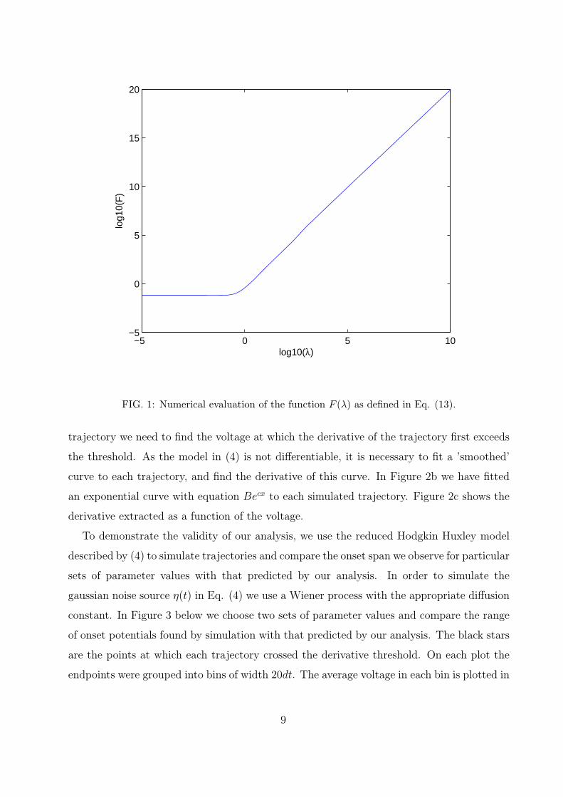
(12) is the central result of this paper, directly relating the onset span S to the noise strength

D, the voltage threshold σ and the onset rapidity a. Fig. 1 shows a numerical evaluation of

F (λ).

Asymptotic analysis of the integral in Eq. (12) shows that at small λ, F (λ) → 0.0629,

and at large λ, F (λ) ∼ λ2/4 (Fig. 1). Hence we obtain

S → 0.2508

√D

aas λ→ 0, (14)

S → σ

2aas λ→∞. (15)

We note that the low λ limit describes the behavior of a simple random walk; here a small

value of λ corresponds to a low threshold for the derivative. Thus the variance of onset

voltages is simply the variance of all possible trajectories the random walk might take. In

the high λ limit the size of the noise term ceases to much affect the variance of onset voltages.

As the derivative threshold is high in this case, the deterministic exponential growth behavior

will dominate those trajectories that reach the threshold.

Thus we have calculated the variance of voltages at which action potential onset occurs

as a function of the onset rapidity a, the onset threshold σ and the level D of synaptic

background activity present. In figure 2a we have simulated a pair of trajectories with

parameter values a = 20ms−1 and D = 1mV2ms−1, and in figure 2d a pair with parameter

values a = 20ms−1 and D = 400mV2ms−1. To ascertain the onset potential of each simulated

8

−5 0 5 10−5

0

5

10

15

20

log10(λ)

log1

0(F

)

FIG. 1: Numerical evaluation of the function F (λ) as defined in Eq. (13).

trajectory we need to find the voltage at which the derivative of the trajectory first exceeds

the threshold. As the model in (4) is not differentiable, it is necessary to fit a ’smoothed’

curve to each trajectory, and find the derivative of this curve. In Figure 2b we have fitted

an exponential curve with equation Becx to each simulated trajectory. Figure 2c shows the

derivative extracted as a function of the voltage.

To demonstrate the validity of our analysis, we use the reduced Hodgkin Huxley model

described by (4) to simulate trajectories and compare the onset span we observe for particular

sets of parameter values with that predicted by our analysis. In order to simulate the

gaussian noise source η(t) in Eq. (4) we use a Wiener process with the appropriate diffusion

constant. In Figure 3 below we choose two sets of parameter values and compare the range

of onset potentials found by simulation with that predicted by our analysis. The black stars

are the points at which each trajectory crossed the derivative threshold. On each plot the

endpoints were grouped into bins of width 20dt. The average voltage in each bin is plotted in

9

0 0.1 0.2 0.30

5

10

15

20

Time (ms)

Vol

tage

(m

V)

0 0.1 0.2 0.30

5

10

15

20

Time (ms)

Vol

tage

(m

V)

0 5 10 15 200

50

100

150

200

Voltage (mV)

Der

ivat

ive

(mV

ms−

1 )

0 0.05 0.1 0.15 0.20

5

10

15

20

Time (ms)

Vol

tage

(m

V)

0 0.05 0.1 0.15 0.20

5

10

15

20

Time (ms)

Vol

tage

(m

V)

0 10 200

50

100

150

200

Voltage (mV)

Der

ivat

ive

(mV

ms−

1 )

d

b c

e f

a

FIG. 2: Pairs of trajectories simulated using (4) with a) onset rapidity a = 20ms−1 and noise

D = 1mVms−1 and d) a = 20ms−1 and D = 400mVms−1. b,e) As described in the text, an

exponential curve was fit to each of the trajectories simulated. c,f) The calculated derivative of

the trajectories in a) and d) plotted as function of the voltage.

magenta, while the mean onset voltage at the center of each bin as predicted by our analysis

is plotted in red. Similarly the standard deviation about the mean in each bin is plotted

in cyan, and can be compared with the standard deviation predicted by our analysis which

has been plotted in green. We observe that both the mean onset potential and the standard

deviation about the mean at each time point found in the simulations is well matched by

that predicted by our analysis.

In both the low λ limit and the high λ limit we found in Eq. (14) that there is indeed an

antagonistic relationship between S and a, as argued by Naundorf et. al [2]. They observed

that changing the parameters of the activation curve and the peak sodium conductance

led to antagonistic changes in the onset rapidity and the onset span; hence they were not

able to fit the Hodgkin-Huxley model to their data. Equations (14) and (15) show that the

antagonistic relationship between S and a is controlled by D in the limit of low λ, and σ

10

0 0.1 0.2 0.3 0.4 0.50

1

2

3

4

5

6

7

8

Time (ms)

Vol

tage

(m

V)

0 0.1 0.2 0.3 0.4 0.50

1

2

3

4

5

6

7

8

Time (ms)

Vol

tage

(m

V)

a b

FIG. 3: Trajectories (10000) were simulated as in 2 with the following sets of parameter values: a)

σ = 25 mVms−1, D = 1 mV2ms−1 and a = 10 ms−1, b) σ = 50 mVms−1, D = 25 mV2ms−1 and

a = 10 ms−1. On each plot the endpoints were grouped into bins of width 20dt. The average voltage

in each bin is plotted in magenta, this should be compared with the most likely onset voltage at

each time point according to our analysis, plotted in red. Similarly the standard deviation in each

bin is plotted in cyan, and can be compared with the standard deviation predicted by our analysis

at each time point, plotted in green.

in the limit of high λ. Neither D (the variance of the synaptic noise strength) nor σ (the

criterion for the voltage threshold) were varied in the simulations of Naundorf et. al [2]. We

observe that our analysis can also be applied to the cooperative model proposed in [2] in

which the probability of channel opening depends on both the membrane voltage and the

local channel density. In the vicinity of the unstable fixed point, incorporating the local

channel density alters the value of a, but does not change the form of equation (4).

We now compare the theory to the results of Naundorf. In their experiments, they mea-

11

10 20 30 40 50 60 70 80 90 1000

2

4

6

8

10

12

14

16

18

20

D = 25(mV2ms−1)

D = 100(mV2ms−1)

D = 400(mV2ms−1)

D = 900(mV2ms−1)Simulation dataRegular spikingFast rhythmic burstingFast spiking

FIG. 4: Here the solid blue dots are the simulation data points reported in [2], while the solid

red, yellow and green dots are the experimental data points from [2] for cat visual cortex neurons

classified electrophysiologically as regular spiking, fast rhythmic bursting, and fast spiking respec-

tively. Data from many cells of each type is displayed in this plot. The curves show our analytical

results for various values of the parameter D.

sure the onset span as the difference between the maximum and minimum voltage threshold

that is measured. Since 99.7% of observations fall within three standard deviations of the

mean, we can approximate the onset span of between 50 and 500 trials as six times the stan-

dard deviation S. We assume that the calculation of the onset span from the simulations in

Naundorf was done in the same fashion.

In Figure 4 we have calculated the onset span as a function of a using different values of

D. Changing the noise strength allows the theoretical curves to move between the various

regimes observed experimentally. For most of the curves through the experimental data,

a noise diffusion constant D = 25 − 100mV2ms−1 fits the data well. Although this is a

larger diffusion constant than that apparently used in the simulations of Naundorf et. al,

this value does a good job of emulating the experimental trajectories shown in Figures 2b

12

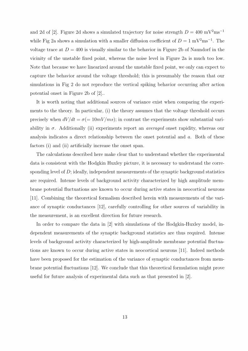
and 2d of [2]. Figure 2d shows a simulated trajectory for noise strength D = 400 mV2ms−1

while Fig 2a shows a simulation with a smaller diffusion coefficient of D = 1 mV2ms−1. The

voltage trace at D = 400 is visually similar to the behavior in Figure 2b of Naundorf in the

vicinity of the unstable fixed point, whereas the noise level in Figure 2a is much too low.

Note that because we have linearized around the unstable fixed point, we only can expect to

capture the behavior around the voltage threshold; this is presumably the reason that our

simulations in Fig 2 do not reproduce the vertical spiking behavior occurring after action

potential onset in Figure 2b of [2]..

It is worth noting that additional sources of variance exist when comparing the experi-

ments to the theory. In particular, (i) the theory assumes that the voltage threshold occurs

precisely when dV/dt = σ(= 10mV/ms); in contrast the experiments show substantial vari-

ability in σ. Additionally (ii) experiments report an averaged onset rapidity, whereas our

analysis indicates a direct relationship between the onset potential and a. Both of these

factors (i) and (ii) artificially increase the onset span.

The calculations described here make clear that to understand whether the experimental

data is consistent with the Hodgkin Huxley picture, it is necessary to understand the corre-

sponding level of D; ideally, independent measurements of the synaptic background statistics

are required. Intense levels of background activity characterized by high amplitude mem-

brane potential fluctuations are known to occur during active states in neocortical neurons

[11]. Combining the theoretical formalism described herein with measurements of the vari-

ance of synaptic conductances [12], carefully controlling for other sources of variability in

the measurement, is an excellent direction for future research.

In order to compare the data in [2] with simulations of the Hodgkin-Huxley model, in-

dependent measurements of the synaptic background statistics are thus required. Intense

levels of background activity characterized by high-amplitude membrane potential fluctua-

tions are known to occur during active states in neocortical neurons [11]. Indeed methods

have been proposed for the estimation of the variance of synaptic conductances from mem-

brane potential fluctuations [12]. We conclude that this theoretical formulation might prove

useful for future analysis of experimental data such as that presented in [2].

13

E. Acknowledgements

This research was supported by the NSF Division of Mathematical Sciences. The writing

of the paper was done in part at the Kavli Institute for Theoretical Physics, also supported

by NSF.

F. References

[1] Hodgkin A, Huxley AF (1952) A quantitative description of membrane current and its appli-

cation to conduction and excitation in nerve. J Physiol 117: 500-544.

[2] Naundorf B, Wolf F, Volgushev M (2006) Unique features of action potential initiation in

cortical neurons. Nature 440: 1060-1063.

[3] McCormick D A, Shu Y, Yu, Y (2007) Hodgkin and Huxley model - still standing? Nature

445: E1-E2.

[4] Naundorf B, Wolf F, Volgushev M (2007) Discussion and Reply. Nature 445: E2-E3.

[5] Destexhe A, Pare D (1999) Impact of network activity on the integrative properties of neo-

cortical pyramidal neurons in vivo. J Neurophysiol 81: 1531-1547.

[6] Destexhe A, Rudolph M, Fellous J-M, Sejnowski T (2001) Fluctuating synaptic conductances

recreate in vivo-like activity in neocortical neurons. Neuroscience 107: 13-24.

[7] Uhlenbeck GE, Ornstein LS (1930) On the theory of the Brownian motion. Phys Rev 36:

823-841.

[8] Hille B (2001) Ion channels of excitable membranes. Sunderland (Massachusetts): Sinauer.

[9] Koch C (1999) Biophysics of Computation: Information Processing in Single Neurons. Oxford:

Oxford University Press.

[10] Feynman RP, Hibbs AR (1965) Quantum mechanics and path integrals. New York: McGraw-

Hill.

[11] Destexhe A, Rudolph M, Pare D (2003) The high-conductance state of neocortical neurons in

vivo. Nature Rev Neurosci 4: 739-751.

[12] Rudolph M, Piwkowska Z, Badoual M, Bal T, Destexhe A(2004) A method to estimate synap-

14

tic conductances from membrane potential fluctuations. J Neurophysio 91: 2884-2896.

G. Figure Legends

Fig 1: Numerical evalution of the function F (λ) as defined in (13) above.

Fig 2: Pairs of trajectories simulated using (4) with a) onset rapidity a = 20ms−1 and

noise D = 1mVms−1 and d) a = 20ms−1 and D = 400mVms−1. b,e) As described in the

text, an exponential curve was fit to each of the trajectories simulated. c,f) The calculated

derivative of the trajectories in a) and c) plotted as function of the voltage.

Fig 3:Trajectories (10000) were simulated as in 2 with the following sets of parameter

values: a) σ = 25 mVms−1, D = 1 mV2ms−1 and a = 10 ms−1, b) σ = 50 mVms−1, D = 25

mV2ms−1 and a = 10 ms−1. On each plot the endpoints were grouped into bins of width

20dt. The average voltage in each bin is plotted in magenta, this should be compared with

the most likely onset voltage at each time point according to our analysis, plotted in red.

Similarly the standard deviation in each bin is plotted in cyan, and can be compared with

the standard deviation predicted by our analysis at each time point, plotted in green.

Fig 4: Here the solid blue dots are the simulation data points reported in [2], while the

solid red, yellow and green dots are the experimental data points from [2] for cat visual

cortex neurons classified electrophysiologically as regular spiking, fast rhythmic bursting,

and fast spiking respectively. Data from many cells of each type is displayed in this plot.

The curves show our analytical results for various values of the parameter D.

15