NEIGHBORHOOD ATTRIBUTES AND COMMUTING BEHAVIOR: TRANSIT CHOICE

Final Report

Metrans Project 03-20

October, 2004

Peter Gordon

School of Policy, Planning, and Development and Department of Economics

Bumsoo Lee School of Policy, Planning, and Development and Department of Economics

James E. Moore II

Department of Industrial and Systems Engineering and Department of Civil Engineering and School of Policy, Planning, and Development

Harry W. Richardson

School of Policy, Planning, and Development and Department of Economics

Christopher Williamson Research Associate Professor of Geography

School of Policy, Planning, and Development University of Southern California

Los Angeles, California 90089-0626

Disclaimer

The contents of this report reflect the views of the authors who are responsible for the facts and the accuracy of the information presented herein. This document is disseminated under the sponsorship of the Department of Transportation, University Transportation Centers Program, and California Department of Transportation in the interest of information exchange. The U.S. Government and California Department of Transportation assume no liability for the contents or use thereof. The contents do not necessarily reflect the official views or policies of the State of California or the Department of Transportation. This report does not constitute a standard, specification, or regulation.

1

Abstract

Neighborhood type matters when we try to explain variations in public transit commuting. We found this statistical link over a sample of all census tracts in the four largest California metro areas. In this research, we used statistical cluster analysis to identify twenty generic neighborhood types. The variables used in the analysis included broad indicators of location and population density, street design, transit access and highway access. Once identified, the denser neighborhoods had higher transit use, other things equal. Yet, what distinguishes the research is that we did not use a simple density measure to differentiate neighborhoods. Rather, density was an important ingredient of our neighborhood-type definition -- which surpassed simple density in explanatory power.

2

Table of Contents

Disclaimer…………………………………………………………………………... 1 Abstract……………………………………………………………………………… 2 Table of Contents…………………………………………………………………… 3 List of Figures and Tables…………………………………………………………... 4 Disclosure…………………………………………………………………………… 4 Introduction…………………………………………………………………………. 5 Neighborhoods……………………………………………………………………… 5 Research Approach….…………………………………………………………….... 10 Data……………………………………………………………………………..... 10 Statistical Cluster Analysis………………………………………………………. 12 Multiple Regression……………………………………………………………… 15 Discussion…………………………………………………………………………… 18 Further Work………………………………………………………………………... 19 References…………………………………………………………………………… 28 Appendix…………………………………………………………………………….. 29

3

List of Figures Figure A1. Histogram of transit user counts Figure A2-a. Geographical clustering of neighborhood types in Los Angeles Figure A2-b. Geographical clustering of neighborhood types of more urbanized areas in Los Angeles

List of Tables

Table 1. OLS regression results of transit use models, 2000 Table 1a. Base models Table 1b. Models with population density Table 1c. Models with neighborhood type dummies Table 2. Negative binominal regression results of transit use models, 2000 Table 2a. Base models Table 2b. Models with population density Table 2c. Models with neighborhood type dummies Table 3. OLS Regression results of transit use change models, 1990-2000 Table 3a. Base models Table 3b. Models with population density Table 3c. Models with population density change Table 3d. Models with neighborhood type dummies Table A1. Neighborhood attributes measures used in the cluster analysis Table A2. Mean values by each neighborhood type (sorted by population density) Table A3. Ranks of neighborhood types by each different variable

Disclosure This project was funded in entirety under this contract to California Department of

Transportation

4

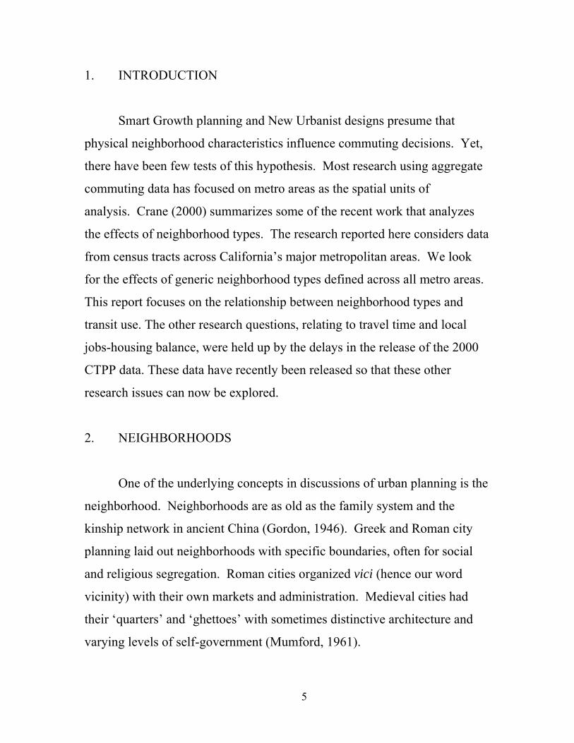
1. INTRODUCTION

Smart Growth planning and New Urbanist designs presume that

physical neighborhood characteristics influence commuting decisions. Yet,

there have been few tests of this hypothesis. Most research using aggregate

commuting data has focused on metro areas as the spatial units of

analysis. Crane (2000) summarizes some of the recent work that analyzes

the effects of neighborhood types. The research reported here considers data

from census tracts across California’s major metropolitan areas. We look

for the effects of generic neighborhood types defined across all metro areas.

This report focuses on the relationship between neighborhood types and

transit use. The other research questions, relating to travel time and local

jobs-housing balance, were held up by the delays in the release of the 2000

CTPP data. These data have recently been released so that these other

research issues can now be explored.

2. NEIGHBORHOODS

One of the underlying concepts in discussions of urban planning is the

neighborhood. Neighborhoods are as old as the family system and the

kinship network in ancient China (Gordon, 1946). Greek and Roman city

planning laid out neighborhoods with specific boundaries, often for social

and religious segregation. Roman cities organized vici (hence our word

vicinity) with their own markets and administration. Medieval cities had

their ‘quarters’ and ‘ghettoes’ with sometimes distinctive architecture and

varying levels of self-government (Mumford, 1961).

5

In the relatively recent history of urban America, the idea of explicitly

using the neighborhood unit to promote health and cultural values was

related to acculturating America’s large immigrant population to be good

citizens and industrial workers (Perry, 1939). Inspired by the experience of

living in New York’s Forest Hills Gardens, social planner Clarence Perry

proposed “neighborhood units” as part of the 1929 Regional Plan for New

York. Perry conceived of the neighborhood as the building block of urban

growth, a self-contained closed system. These are reflective of common

sense approaches that refer to the beginning of the street car suburbs of the

late 19th Century, the garden city movement in the United Kingdom, and a

reaction against dense immigrant housing in America. Perry’s ideas

received the backing of the then recently established Federal Housing

Administration (FHA) which sent out brochures nationwide describing the

concept to developers. However, developers tended to focus on housing

construction rather than on neighborhood civic and commercial uses,

undercutting one of Perry’s goals and reinforcing the segregation of land

uses that make automobile travel attractive even for short neighborhood trips

(ICMA, 2000).

Perry identified six attributes in his neighborhood model:

1. Size – based on elementary school average attendance (about 400

children) to which children can walk without crossing major streets. The precise area would depend on residential density and the amount of non-residential land uses. An average population would be about 7,000, or about 2,000 housing units. (This measure implies assumptions regarding the number of children per household, household age distribution, household size, fertility rates of child-bearing age women, and that most children attend public school.)

6

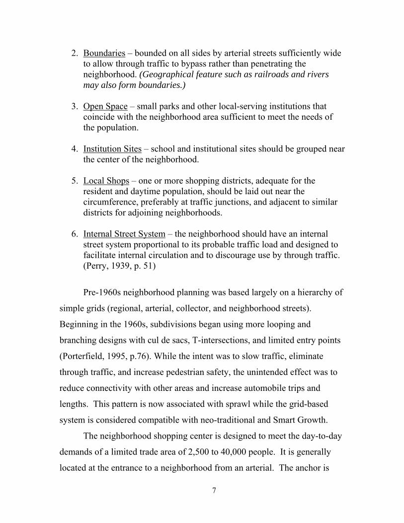
2. Boundaries – bounded on all sides by arterial streets sufficiently wide to allow through traffic to bypass rather than penetrating the neighborhood. (Geographical feature such as railroads and rivers may also form boundaries.)

3. Open Space – small parks and other local-serving institutions that

coincide with the neighborhood area sufficient to meet the needs of the population.

4. Institution Sites – school and institutional sites should be grouped near

the center of the neighborhood. 5. Local Shops – one or more shopping districts, adequate for the

resident and daytime population, should be laid out near the circumference, preferably at traffic junctions, and adjacent to similar districts for adjoining neighborhoods.

6. Internal Street System – the neighborhood should have an internal

street system proportional to its probable traffic load and designed to facilitate internal circulation and to discourage use by through traffic. (Perry, 1939, p. 51)

Pre-1960s neighborhood planning was based largely on a hierarchy of

simple grids (regional, arterial, collector, and neighborhood streets).

Beginning in the 1960s, subdivisions began using more looping and

branching designs with cul de sacs, T-intersections, and limited entry points

(Porterfield, 1995, p.76). While the intent was to slow traffic, eliminate

through traffic, and increase pedestrian safety, the unintended effect was to

reduce connectivity with other areas and increase automobile trips and

lengths. This pattern is now associated with sprawl while the grid-based

system is considered compatible with neo-traditional and Smart Growth.

The neighborhood shopping center is designed to meet the day-to-day

demands of a limited trade area of 2,500 to 40,000 people. It is generally

located at the entrance to a neighborhood from an arterial. The anchor is

7

typically a grocery store with adjacent drug stores, small retail and service

establishments, and restaurants. A typical center would be 50,000 square

feet (but could range between 30,000 to 100,000, depending on the trade

area population) and require 3 to 10 acres (Porterfield, 1995).

Jane Jacobs questions some aspects of the neighborhood concept in

her classic critique of urban planning, The Death and Life of Great American

Cities. She argues that city residents are mobile and pick and choose from

the entire city (and beyond). They are not restricted to the provincialism of a

neighborhood (Jacobs, 1961). This critique was written over 40 years ago in

the middle of the Baby Boom when most households had one car and when,

the suburbs were in their first phase of post-war expansion.

Baer and Banerjee (1984) expanded Perry’s definition, adding three

aspects:

Context: The neighborhood ‘movement’ was a turn-of-the-century (1900) outgrowth of the concern over urban lifestyle and its weakening of the traditional links between the individual, the place, and community (White and White, 1962). The erosion of the family and the general moral order was thought to be a function of the lack of dignity and community found in industrial city housing, which were generally described as impersonal and unhealthy. This approach might be seen as “social engineering” and “assimilation of immigrants.” It is reflected in today’s preference for home ownership and the single family house.

Manifest: Perry (1952) recognized early that the automobile was the

chief ‘villain’ that the neighborhood unit was trying to counterbalance, with an emphasis on a walkable radius focused on the school and surrounding civic and retail functions. This concept was perhaps first realized in Radburn and other garden cities (Stein, 1957).

Tacit: Uniformity of design, scale, and people was an underlying

assumption. The emphasis on child-rearing (especially young children)

8

spilled over into economic and racial homogeneity. This policy was explicitly enforced by covenants and FHA lending practices into the 1950s.

The neighborhood has become a prototypical planning element of the

American suburban city and a standard ‘product’ of developers and

merchant builders. Today’s new neighborhoods typically have entry and

image treatments and/or may be gated. The better plans included a

neighborhood park near the center, perhaps adjacent to the school. Many

are developed with Home Owners Associations, with extensive landscaping

and regulations for painting and maintenance, and perhaps a swimming pool

and other facilities.

The classic neighborhood unit could not have been intended to capture

the majority of the work-related trips internally, as it included only a small

amount of non-residential land uses. But, in theory, it would capture trips to

elementary schools, neighborhood retail stores, and neighborhood civic uses

such as attending church or visiting a park. The question, then, seems to be

whether Perry’s ‘neo-traditional’ neighborhood model ever worked

(assuming it was developed and tested) or have so many residents changed

their reasons and destinations for travel that the classic neighborhood model

simply does not capture their destinations as well as it used to, even if it

were built according to the classic definition? This research effort attempts

to answer that question in California, by defining a range of neighborhoods

from Perry’s classic model (which may include New Urbanist developments

and older suburbs) to new, sprawling suburbs.

9

3. RESEARCH APROACH

A. DATA

The purpose of this research is to test how physical neighborhood

characteristics influence commuting decisions, especially transportation

mode choice, where choice exists and, commuting time. So far, we have

examined commuting mode choice.

We relied on journey-to-work data from the U.S. decennial census to

analyze commuting behavior at the census tract level for California’s four

biggest metro areas, Los Angeles, San Francisco, San Diego and Sacramento.

Several census tract-level social, economic and housing characteristics data

are taken from the 1990 and 2000 Census Summary File 3 (STF3).

One standard problem in using the census data over time is that census

geography changes significantly across census years, especially at a small

geographic scale. The Census Neighborhood Change Database (NCDB)

1970-2000 Tract Data, provided by GeoLytics and the Urban Institute,

enabled us to overcome the geographic comparability problem by remapping

earlier census year data to 2000 census tract boundaries. Therefore, all

census variables for any census year in this report are presented for 2000

census geography.

Measures of physical neighborhood characteristics that are critical in

testing our research questions were not readily available. However, we

derived many of the required variables using geographical information

systems (GIS). The 2000 TIGER® (Topologically Integrated Geographic

Encoding and Referencing system) street networks files were used to

measure street design, which has often been suggested as associated with

10

local and regional accessibility, and hence affect commuting behavior. In

addition to the TIGER files, GIS map data of rail transit lines were obtained

from each metropolitan planning organization (MPO) of our study areas and

are used to measure rail transit access.

11

B. STATISTICAL CLUSTER ANALYSIS

The strategy we adopted to test physical neighborhood characteristics’

influence on commuting decisions involved two steps. First, we classified

all census tracts in our study areas into twenty prototypical neighborhood

categories using a statistical cluster analysis. Smith and Saito’s (2001)

results suggested that meaningful spatial aggregates can be identified via this

approach. In an analysis of local area characteristics and their effects on

mode choice, Srinivasan (2002) gathered data on these variables for Boston

area TAZs. In contrast, we first investigated which census tracts cluster into

meaningful neighborhood units.

In the next step, we tested influences on commuting decisions of

these neighborhood types as well as those of traditional explanatory

variables; as an example, for mode choice it is logical to test the influence of

household income.

We used ten physical descriptor variables in the cluster analysis.

These included measures of the contextual position, street design, and transit

and highway access of each census tract (Table A1). Population density,

distance from the core-CBD of each metropolitan area, and the age of

housing stock are basic variables for a census tract. Street design variables,

such as street density, intersection density, and the cul-de-sac ratio, are

expected to be associated with pedestrian access, intra-neighborhood

connectivity, and ultimately automobile dependence. These factors are

considered especially important in New Urbanist neighborhood design.

Access to such major transportation infrastructure as rail transit systems,

park and ride stations, and highways would also affect commuting behavior.

Bus transit access, however, is not taken into account in classifying

12

neighborhood types on the ground that bus routes are highly ubiquitous and

very flexible. Hence, they are endogenous to transit demand rather than

being exogenous.

All these variables, except population density and the median age of

the housing stock that are directly available from the Census STF3 file, are

derived from TIGER street networks files and GIS map files of each

metropolitan area’s rail transit system. We pooled all 5,727 census tracts

data in the four study areas, excluding ones on islands and ones without

commuters. We then performed cluster analysis to seek generic California

neighborhood prototypes across the four metropolitan areas.

Whereas a variety of techniques are available for cluster analysis, we

have chosen perhaps the most commonly used methods in this field1:

Euclidean distance is used as a similarity measure, and Ward’s minimum-

variance method is used as a hierarchical clustering technique. We

standardized the distributions of all variables to normal distributions before

conducting the cluster analysis. Twenty clusters or neighborhood types were

determined by evaluating the statistical clusters ex post. Reasonable size

distributions of clusters and their spatial distribution, and how many clusters

were manageable were considered in making the decision. Some

arbitrariness is inevitable given that such statistics such as the Cubic

Clustering Criterion (CCC), the Pseudo F-statistic (PSF), and the Pseudo-t2

statistic do not clearly indicate an optimal number of clusters. All data

analyses used procedures provided by the SAS software package. The

1 A study attempting to classify 343 planning districts in Utah’s Wasatch Front region to 35 land-

use distribution scenarios found after applying a series of cluster analysis options that a combination of the Ward’s linkage method and the Squared Euclidean distance measure produced the most reasonable outcome (Smith and Saito, 2001).

13

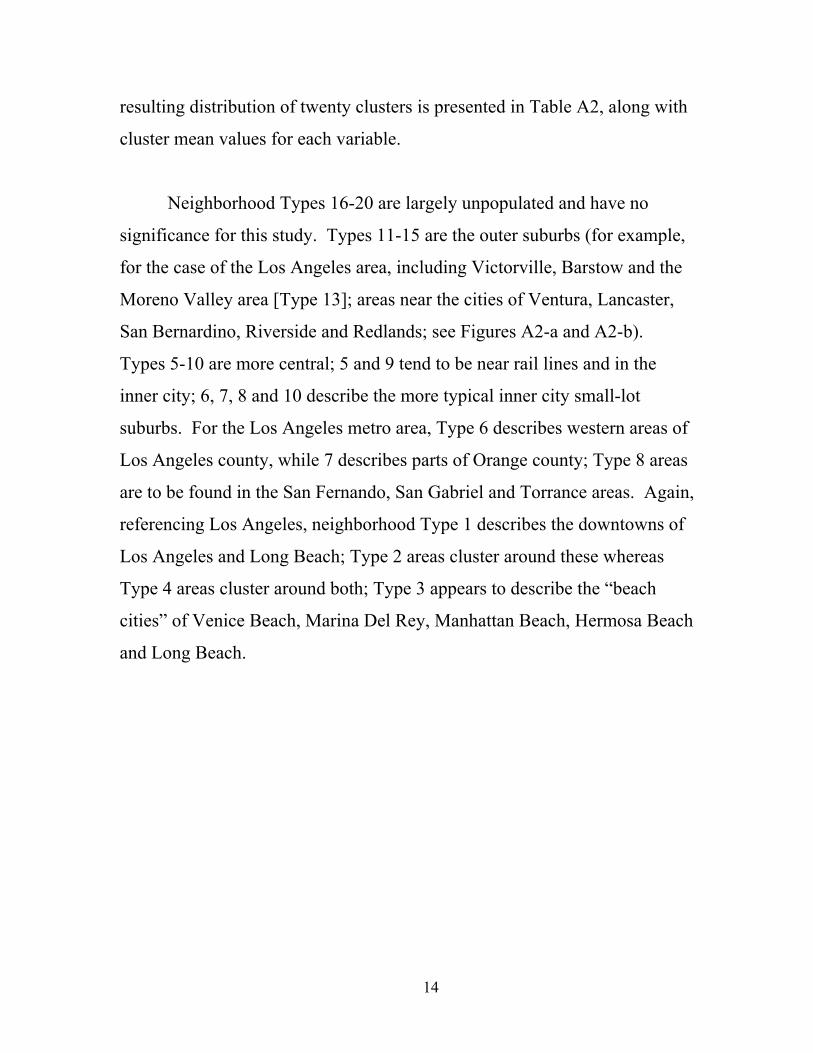
resulting distribution of twenty clusters is presented in Table A2, along with

cluster mean values for each variable.

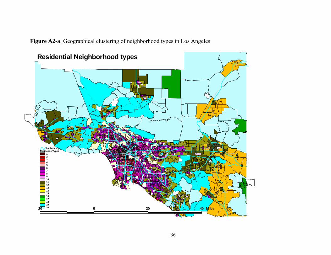
Neighborhood Types 16-20 are largely unpopulated and have no

significance for this study. Types 11-15 are the outer suburbs (for example,

for the case of the Los Angeles area, including Victorville, Barstow and the

Moreno Valley area [Type 13]; areas near the cities of Ventura, Lancaster,

San Bernardino, Riverside and Redlands; see Figures A2-a and A2-b).

Types 5-10 are more central; 5 and 9 tend to be near rail lines and in the

inner city; 6, 7, 8 and 10 describe the more typical inner city small-lot

suburbs. For the Los Angeles metro area, Type 6 describes western areas of

Los Angeles county, while 7 describes parts of Orange county; Type 8 areas

are to be found in the San Fernando, San Gabriel and Torrance areas. Again,

referencing Los Angeles, neighborhood Type 1 describes the downtowns of

Los Angeles and Long Beach; Type 2 areas cluster around these whereas

Type 4 areas cluster around both; Type 3 appears to describe the “beach

cities” of Venice Beach, Marina Del Rey, Manhattan Beach, Hermosa Beach

and Long Beach.

14

C. MULTIPLE REGRESSIONS

Multiple regression analyses were done to test neighborhood type effects on

commuting mode choices. The dependent variable of our regression models,

the number of transit users in each census tract, is a count variable, which

takes on nonnegative integer value or zero in many incidences. Hence, the

Poisson or negative binomial regression model is more appropriate for our

data, because linear models by ordinary least square (OLS) estimation may

predict negative counts.

The Poisson regression model assumes that the count variable of interest, the

number of transit users in our case, follows a Poisson distribution:

iii

yi

i xwhereyy

eyYprob

ii

'ln,...,1,0,!

)( βλλλ

====−

The maximum likelihood estimator of the coefficients is the semielasticity of

E(y|x) with respect to a covariate (Wooldridge, 2002). That is, the

percentage change in E(y|x) can be approximated by 100βj*∆xj, for a small

change ∆xj. Cameron and Windmeijer (1996)’s measure based on the

deviances is often used to evaluate the goodness of fit:

∑

∑

=−

=∧

−= n

i

ii

n

ii

ii

d

y

yy

yy

R

1

12

)ln(

)ln(

1 λ

However, the Poisson regression model’s strong assumption that the

conditional variance equals the mean is very often violated. Transit user

counts in our data are also overdispersed. As shown in Figure A1, the

15

variance is over 250 times larger than the mean. A common alternative in

overdispersion cases is the negative binomial regression model, which

allows the variance to differ from the mean,

εβλ += ii x'ln , where exp(ε) follows a gamma distribution with mean 1

and variance α.

Data for the year 2000 for our variables of interest were compiled and

examined for the 5,727 census tracts in the Los Angeles, San Francisco, San

Diego and Sacramento MSAs. Results for both OLS and negative binomial

regressions for the pooled data set and for each MSA are reported below.

The two sets of results are very similar and in what follows, only the OLS

findings are discussed

OLS regression results are shown in Table 1 (corresponding negative

binomial results are shown in Table 2). At the census tract level, the number

of transit commuters is explained by the total number of commuters and by

how many are below the poverty line. Metro area dummy variables add a

negative influence if the census tract is not in the San Francisco area. All

the signs are as expected with very large t-values. Forty percent of the

variation of the dependent variable is explained. The model for pooled

metro areas explains more than the individual area models, with the

exception of Los Angeles.

The explanatory power of these models is improved, as expected, if census

tract population densities are added (Table 1b). Higher density tracts

account for more transit commuting. Models using the pooled data as well

16

as models for Los Angeles and San Diego explain more than fifty percent of

the variation of the dependent variable.

The results in Table 1c show that neighborhood type matters. Replacing the

density variable with all the neighborhood type variables boosts the

explanatory power of the models. Also, all the neighborhood type dummy

variables have large t-values except for Type 3 (neighborhood Type 8 is the

reference type). The neighborhood types are listed in the order of their

average population density (which, reasonably, correlates with street

densities). As expected, almost all of the dense types have positive signs

while all of the less dense types have negative signs. This model is superior

to the models in Table 1b, not only because more variance of the dependent

variable is explained but also because neighborhood type includes much

more information than population density alone.

Yet, the neighborhoods identified vary along various other interesting

dimensions. Whereas Types 1 and 2 were the densest, Type 1 is limited to

downtown areas of Los Angeles and Long Beach; Type 2 describes areas

nearby these centers but also found in central parts of Glendale and Santa

Ana.

It is also noteworthy that the improvement in statistical fit for the four other

metro areas improves to the point where all are almost equally able to

explain transit commuting. With rare exceptions, neighborhood types have

similar effects across metro areas.

17

Trying to explain the ten-year change in transit use (1990-2000) at the small-

area level is less successful. Table 3a shows tests that mirror those reported

in Table 1a with the dependent variable being the 1990-2000 change in

transit commuting. Independent variables include the change in the number

of commuters and the change in the number of people in poverty. This is

where the GeoLytics software described earlier was useful. The number of

census tracts studied was slightly fewer (5680) reflecting the fact that a few

1990 tracts had no commuters. The signs of all three independent variables

(and the three dummy variable coefficients) are as expected with high t-

values. Yet, only 11 percent of the cross-section’s variation of transit

commuting is explained for the pooled sample. Individual metro area

models provide similar results.

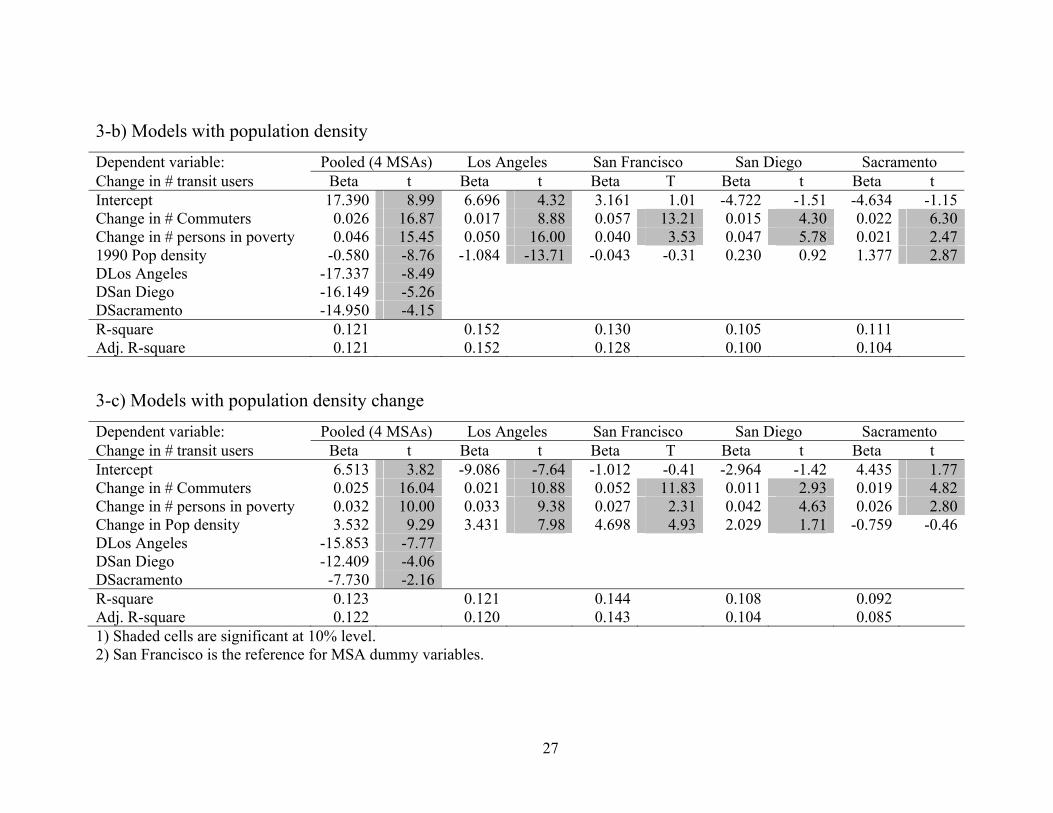
Adding 1990 census tract population densities (Table 3b) yields mixed

results. For the pooled sample and for the Los Angeles area, higher densities

have a negative effect on transit use once the effects of other variables are

accounted for.

Results in Table 3c show what happens when 1990 densities are replaced

with the ten-year change in densities. This time as densities increase, so

does transit use. This effect was also found for all areas but Sacramento.

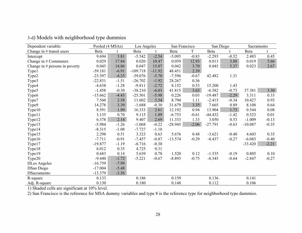
Table 3d results show the density variables replaced by the neighborhood

type dummy variables for 2000; these are again ranked (labeled) by average

population density. Only some of these are significant and there is no

apparent pattern in terms of their density variation.

18

4. DISCUSSION

Our results support the idea that neighborhood type matters when it

comes to transit commuting. This does not imply that neighborhood change

as a policy is cost-effective or worth pursuing. Such a strategy, even if

feasible, would take too long. It suggests, however, that at the margin,

transit commuting impacts and neighborhood type are interdependent.

Nevertheless, the politicized placement of many of the recently installed rail

transit stations in California (Altshuler and Leberoff, 2003, Ch.6) suggests

that it is reasonable to test one-way causation.

5. FURTHER WORK

We plan to extend our research along similar lines to the study of the

variations in commuting time. We will use the same neighborhood types.

We will also investigate the impacts of destination neighborhood types The

(default) competing variable will be each census tract’s conventionally

calculated regional job accessibility index. This variable will be computable

by using the CTPP data for the four metro areas.

Given the finding that our neighborhood types can explain variations

in transit commuting, even when the impacts of poverty levels are held fixed,

can they also explain variations in commuting times, when the impacts of

job accessibility are held fixed?

We also intend to examine whether the identified neighborhoods lend

any credence to the concept of local jobs-housing balance. Still another

19

direction for further work would be an investigation of alternate definitions

neighborhood types and their consequences.

20

Table 1. OLS regression results of transit use models, 2000

1-a) Base models Dependent variable: Pooled (4 MSAs) Los Angeles San Francisco San Diego Sacramento Log of # transit users

Obs. 5727

Obs. 3307

Obs. 1430

Obs. 593

Obs. 397

Beta t Beta t Beta t Beta t Beta tIntercept -2.0487 -8.99 -3.5134 -12.15 -1.7987 -3.99 -3.1968 -4.63 -4.575 -5.49Log of # commuters 0.3389 11.02 0.2670 6.79 0.5236 8.27 0.2841 2.95 0.704 5.96Log of # persons in poverty 0.7383 47.11 0.8510 43.9 0.4436 12.13 0.7895 16.67 0.458 8.09D Los Angeles -1.3075 -33.94 D San Diego -1.2588 -21.94 D Sacramento -1.4284 -21.44

R-square 0.397 0.408 0.192 0.377 0.280Adj. R-square 0.397 0.408 0.191 0.375 0.276

1-b) Models with population density Dependent variable: Pooled (4 MSAs) Los Angeles San Francisco San Diego Sacramento Log of # transit users Beta t Beta t Beta t Beta t Beta t Intercept -0.8690 -4.22 -2.0859 -7.94 -1.0679 -2.67 -2.4557 -4.07 -2.7094 -3.38Log of # commuters 0.2343 8.49 0.1383 3.91 0.4755 8.50 0.2542 3.03 0.5282 4.75Log of # persons in poverty 0.5239 34.75 0.6290 33.26 0.2308 6.80 0.5593 12.57 0.3006 5.41Log of pop density 0.4093 38.16 0.4178 29.06 0.4133 20.21 0.4531 13.76 0.3059 8.32D Los Angeles -1.2692 -36.88 D San Diego -1.1447 -22.31 D Sacramento -1.0692 -17.76

R-square 0.520 0.528 0.372 0.529 0.388Adj. R-square 0.519 0.528 0.371 0.526 0.3831) Shaded cells are significant at 10% level. 2) San Francisco is the reference for MSA dummy variables.

21

1-c) Models with neighborhood type dummies Dependent variable: Pooled (4 MSAs) Los Angeles San Francisco San Diego Sacramento Log of # transit users Beta t Beta t Beta t Beta t Beta tIntercept -1.7089 -8.63 -2.4179 -9.5 -2.4960 -7.13 -3.4481 -5.49 -4.0123 -5.07Log of # commuters 0.4574 16.67 0.2850 7.93 0.7530 14.97 0.5079 5.58 0.8964 8.01Log of # persons in poverty 0.5476 36.80 0.6892 35.37 0.2788 9.49 0.5837 12.09 0.2134 3.86Type1 1.5028 11.17 1.3569 8.43 1.6221 7.19 Type2 1.2316 14.10 0.8708 7.22 1.5172 11.97

0.7554

1.10

Type3 -0.1555 -0.66 -0.1167 -0.48 -0.2360 -0.27Type4 0.6618 11.42 0.5111 7.92 0.9431 5.44 0.6270 2.73

Type5 0.7519 9.87 0.6711 5.99 0.7863 6.12 0.7413 3.69 0.9653 3.34Type6 0.4377 7.93 0.3116 4.22 0.7604 7.89

0.2955 1.59 0.1739 0.69

Type7 -0.3821 -8.37 -0.3118 -5.48 -0.5539 -6.30

-0.1567 -1.02 -0.0086 -0.03Type9 0.2691 4.09 0.3009 3.04 0.1790 1.72 0.3711 1.97 0.5052

1.58

Type10 -0.2518 -3.79 -0.1243 -1.18 -0.4384 -3.04 0.0188 0.11 -0.5899 -3.50Type11 -1.0748 -15.44 -1.1083 -13.19 -1.0546 -8.64 -1.1290 -1.65 -2.1070 -2.06Type12 -0.5442 -11.70 -0.4596 -7.53 -0.5899 -6.27 -0.4637 -3.69 -1.0584 -5.40Type13 -1.4886 -20.46 -1.4868 -18.13 -1.4175 -9.28 -2.0364 -2.12 -3.3576 -4.60Type14 -1.3051 -10.86 -1.3634 -11.3 Type15 -0.2238 -3.17 -0.3624 -3.94 0.2775 2.11 -0.5177 -2.61 -0.5156 -1.55Type16 -2.1977 -16.72 -2.4215 -16.28 -2.6979 -5.28 -3.1561 -4.61 -1.2466 -3.15Type17 -1.0765 -4.14 -2.4564 -6.3 -0.2626 -0.68Type18 -1.9945 -7.35 -2.1785 -8.03

Type19 -0.8117 -10.74 -0.6333 -5.08 -0.5565 -3.96 -1.0986 -6.24 -1.2487 -5.88Type20 -1.8683 -21.92 -1.6776 -12.6 -1.9071 -14.46 -2.4166 -8.57 -1.9642 -7.20D Los Angeles -1.1443 -34.65 D San Diego -1.1375 -23.32 D Sacramento -1.1664 -19.83

R-square 0.593 0.599 0.559 0.539 0.488Adj. R-square 0.591 0.596 0.553 0.526 0.4681) Shaded cells are significant at 10% level. 2) San Francisco is the reference for MSA dummy variables and type 8 is the reference type for neighborhood type dummies.

22

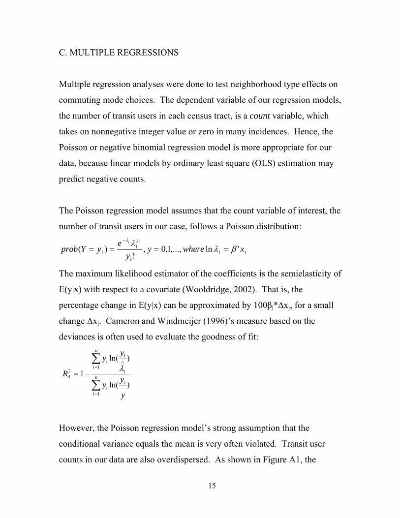
Table 2. Negative binomial regression results of transit use models, 2000

2-a) Base models Dependent variable: Pooled (4 MSAs) Los Angeles San Francisco San Diego Sacramento Log of # transit users

Obs.

5727 Obs.

3307 Obs.

1430 Obs.

593 Obs.

397

Beta Chi-Sq. Beta Chi-Sq. Beta Chi-Sq. Beta Chi-Sq. Beta Chi-Sq.Intercept -5.4680 6020.9 -7.5969 6031.6 -3.8611 618.7 -6.2651 1089.2 -5.4836 477.6Log of # commuters fixed fixed fixed fixed fixedLog of # persons in poverty 0.5511 2114.4 0.7048 2132.1 0.2618 94.4 0.4744 238.0 0.3158 57.8D Los Angeles -1.1495 1112.7 D San Diego -1.2534 610.6 D Sacramento -1.3790 546.8

R-square 0.574 0.552 0.304 0.537 0.416Log-likelihood -31601 -17504 -8990.9 -3041.4 -1936.0Deviance 6909.6 4041.9 1666.6 722.9 485.41) Shaded cells are significant at 10% level. 2) San Francisco is the reference for MSA dummy variables. 3) R-square in negative binomial regression models are measured based on the deviances.

23

2-b) Models with population density Dependent variable: Pooled (4 MSAs) Los Angeles San Francisco San Diego Sacramento Log of # transit users

Obs.

5727 Obs.

3307 Obs.

1430 Obs.

593 Obs.

397

Beta Chi-Sq. Beta Chi-Sq. Beta Chi-Sq. Beta Chi-Sq. Beta Chi-Sq.Intercept -5.1310 5499.5 -7.1347 5599.5 -3.3258 521.1 -6.2210 1070.7 -5.1298 414.6Log of # commuters fixed fixed fixed fixed fixedLog of # persons in poverty 0.3520 715.7 0.4930 860.9 0.0193 0.5 0.3549 112.8 0.1994 20.2Log of pop density 0.3346 1215.8 0.3481 698.9 0.3546 460.2 0.3166 100.8 0.2279 47.3D Los Angeles -1.0743 1115.9 D San Diego -1.1046 546.6 D Sacramento -1.0055 323.8 R-square 0.673 0.635 0.461 0.652 0.503Log-likelihood

-31124 -17229 -8818.3

-3002.0

-1916.2

Deviance 6932.0 4069.7 1648.9 737.6 485.11) Shaded cells are significant at 10% level. 2) San Francisco is the reference for MSA dummy variables. 3) R-square in negative binomial regression models are measured based on the deviances.

24

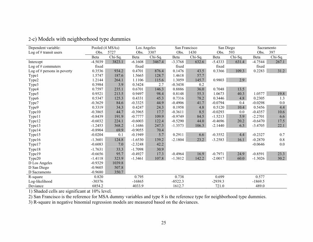
2-c) Models with neighborhood type dummies Dependent variable: Pooled (4 MSAs) Los Angeles San Francisco San Diego Sacramento Log of # transit users

Obs.

5727 Obs.

3307 Obs.

1430 Obs.

593 Obs.

397

Beta Chi-Sq. Beta Chi-Sq. Beta Chi-Sq. Beta Chi-Sq. Beta Chi-Sq.Intercept -4.5039 3823.1 -6.1608 3467.4 -3.3768 632.6 -5.4333 631.4 -4.7544 267.1 Log of # commuters fixed fixed fixed fixed fixedLog of # persons in poverty 0.3536 934.2 0.4701 876.4 0.1476 43.5 0.3366 109.3 0.2283 31.2 Type1 1.5747 187.6 1.5665 128.7 1.4618 57.7

Type2 1.2144 264.1 1.1106 115.6 1.3059 145.7 0.9803 2.9 Type3 0.3984 3.9

0.3424 2.7 -0.3438 0.2Type4 0.7597 235.1 0.6701 146.3 0.8886 36.0 0.7048 13.5

Type5 0.9521 213.5 0.9497 98.4 0.8148 55.3 1.0673 40.3 1.0577 19.8 Type6 0.5347 125.3 0.4331 45.3 0.7316 78.2 0.3446 4.8

0.2305 1.3

Type7 -0.3629 84.6 -0.3325 44.9 -0.4906 41.7

-0.0794 0.4 -0.0298 0.0Type9 0.3319 34.3 0.4247 24.3 0.1958 4.8 0.5120 10.4 0.5456 4.4 Type10 -0.3865 44.7 -0.3965 17.7 -0.3611 8.5 -0.0293 0.0 -0.4357 10.6 Type11 -0.8439 191.9 -0.7777 109.9 -0.9749 84.5 -1.5213 5.9 -2.2701 6.6 Type12 -0.6032 224.1 -0.6003 122.4 -0.5290 44.0 -0.4696 20.2 -0.6470 17.5 Type13 -1.2453 368.2 -1.1686 247.3 -1.3573 106.3 -2.1440 6.3 -3.4705 22.1 Type14 -0.8904 69.9 -0.9055 70.

4

Type15 -0.0204 0.1 -0.1949 5.7 0.2911 6.6 -0.3552 4.4

-0.2327 0.7Type16 -1.3601 124.8 -1.6530 139.2 -2.1804 23.2 -3.2583 16.1

-0.2870 0.8

Type17 -0.6083 7.0 -2.3248 42.2

-0.0646 0.0Type18 -1.7631 33.3 -1.7098 30.9

Type19 -0.6656 95.7 -0.4927 17.3 -0.4964 16.9 -0.7971 24.9 -0.8591 23.3 Type20 -1.4118 323.9 -1.3461 107.8 -1.3812 142.2 -2.0017 60.0 -1.3026 30.2 D Los Angeles -0.9329 1039.8 D San Diego -0.9605 507.8 D Sacramento -0.9680 350.7

R-square 0.820 0.795 0.738 0.699 0.577 Log-likelihood

-30376 -16865 -8522.3 -2939.3 -1869.5

Deviance 6854.2 4033.9 1612.7 721.0 489.01) Shaded cells are significant at 10% level. 2) San Francisco is the reference for MSA dummy variables and type 8 is the reference type for neighborhood type dummies. 3) R-square in negative binomial regression models are measured based on the deviances.

25

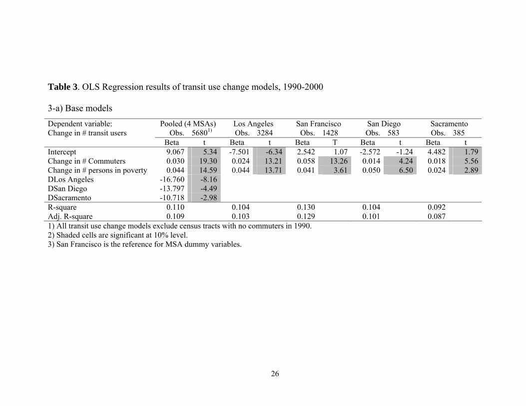
Table 3. OLS Regression results of transit use change models, 1990-2000

3-a) Base models Dependent variable: Pooled (4 MSAs) Los Angeles San Francisco San Diego Sacramento Change in # transit users

Obs. 56801) Obs. 3284

Obs. 1428

Obs. 583

Obs. 385

Beta t Beta t Beta T Beta t Beta tIntercept 9.067 5.34 -7.501 -6.34 2.542 1.07 -2.572 -1.24 4.482 1.79Change in # Commuters 0.030 19.30 0.024 13.21 0.058 13.26 0.014 4.24 0.018 5.56Change in # persons in poverty 0.044 14.59 0.044 13.71 0.041 3.61 0.050 6.50 0.024 2.89DLos Angeles -16.760 -8.16 DSan Diego -13.797 -4.49

DSacramento -10.718 -2.98

R-square 0.110 0.104 0.130 0.104 0.092

Adj. R-square 0.109 0.103 0.129 0.101 0.0871) All transit use change models exclude census tracts with no commuters in 1990. 2) Shaded cells are significant at 10% level. 3) San Francisco is the reference for MSA dummy variables.

26

3-b) Models with population density Dependent variable: Pooled (4 MSAs) Los Angeles San Francisco San Diego Sacramento Change in # transit users Beta t Beta t Beta T Beta t Beta tIntercept 17.390 8.99 6.696 4.32 3.161 1.01 -4.722 -1.51 -4.634 -1.15Change in # Commuters 0.026 16.87 0.017 8.88 0.057 13.21 0.015 4.30 0.022 6.30Change in # persons in poverty 0.046 15.45 0.050 16.00 0.040 3.53 0.047 5.78 0.021 2.471990 Pop density -0.580 -8.76 -1.084 -13.71 -0.043 -0.31 0.230 0.92 1.377 2.87DLos Angeles -17.337 -8.49 DSan Diego -16.149 -5.26

DSacramento -14.950 -4.15

R-square 0.121 0.152 0.130 0.105 0.111

Adj. R-square 0.121 0.152 0.128 0.100 0.104

3-c) Models with population density change Dependent variable: Pooled (4 MSAs) Los Angeles San Francisco San Diego Sacramento Change in # transit users Beta t Beta t Beta T Beta t Beta tIntercept 6.513 3.82 -9.086 -7.64 -1.012 -0.41 -2.964 -1.42 4.435 1.77Change in # Commuters 0.025 16.04 0.021 10.88 0.052 11.83 0.011 2.93 0.019 4.82Change in # persons in poverty 0.032 10.00 0.033 9.38 0.027 2.31 0.042 4.63 0.026 2.80Change in Pop density 3.532 9.29 3.431 7.98 4.698 4.93 2.029 1.71 -0.759 -0.46DLos Angeles -15.853 -7.77 DSan Diego -12.409 -4.06

DSacramento -7.730 -2.16

R-square 0.123 0.121 0.144 0.108 0.092

Adj. R-square 0.122 0.120 0.143 0.104 0.0851) Shaded cells are significant at 10% level. 2) San Francisco is the reference for MSA dummy variables.

27

3-d) Models with neighborhood type dummies Dependent variable: Pooled (4 MSAs) Los Angeles San Francisco San Diego Sacramento Change in # transit users Beta t Beta t Beta T Beta t Beta tIntercept 9.694 3.81 -5.542 -2.54 -5.095 -0.83 -2.293 -0.52 2.483 0.45Change in # Commuters 0.029 17.84 0.020 10.47 0.059 12.93 0.013 3.88 0.019 5.66Change in # persons in poverty 0.045 14.86 0.047 15.07 0.042 3.70 0.045 5.37 0.023 2.67Type1 -59.181 -6.91 -109.718 -11.92 48.451 2.39Type2 -23.597 -4.25 -39.076 -5.70 -7.596

-0.67 42.482 1.31

Type3 -22.831 -26.702-1.51 -1.92 28.267

0.36Type4 -4.638 -1.28 -9.811 -2.72 8.152

0.53 15.200 1.43

Type5 -1.458 -38.210-0.30 -6.03 41.815 3.63 -6.582 -0.73 37.381 3.30Type6 -15.662 -4.43 -25.501 -5.98 0.226 0.03 -19.487 -2.29 3.311 0.33Type7 7.560 2.58 11.602 3.54 8.794

1.11 -2.415 -0.34 10.427 0.93

Type9 14.278 3.39 -1.688 -0.30 31.679 3.35 7.665

0.89 8.108 0.64Type10 8.591 1.99 16.333 2.61 12.192 0.94 13.904 1.73 0.544 0.08Type11 3.135 0.70 9.115 1.89 -6.753

-0.61 -44.432 -1.42 0.523 0.01

Type12 6.378 2.14 9.407 2.69 11.333

1.33 3.050 0.53 -1.009 -0.13Type13 -5.984 -1.26 -1.068 -0.22 -28.945 -2.06 -27.791

-0.63 -10.087 -0.35Type14 -8.315 -1.08 -7.727

-1.10

Type15 2.298 0.51 3.323 0.63 5.676 -3.6210.48 4.603-0.40 0.35Type16 -7.711 -0.91 -7.457 -0.87 -13.574 -0.29 -8.437

-0.27 -6.083 -0.40

Type17 -19.877 -1.19 -6.716 -0.30 -33.420 -2.21Type18

6.012 0.35 4.725 0.31Type19 0.683 0.14 5.639 0.78 1.520 -1.5350.12 0.805-0.19 0.10Type20 -9.440 -1.72 -5.221 -0.67 -8.893 -0.75 -8.345 -0.64 -2.847 -0.27DLos Angeles -16.759 -7 9.9 DSan Diego -17.004 -5 8

.4

DSacramento -13.379 -3 6

.5R-square 0.133 0.186 0.159 0.136 0.141Adj. R-square 0.130 0.180 0.148 0.112 0.1061) Shaded cells are significant at 10% level. 2) San Francisco is the reference for MSA dummy variables and type 8 is the reference type for neighborhood type dummies.

28

29

REFERENCES

Altshuler, Alan and Luberoff, David (2003) Mega-Projects: The Changing Politics of Urban Public Investment. Washington, DC: The Brookings Institution.

Baer, W. and Banerjee, T. (1984) Beyond the Neighborhood Unit: Residential Environments and Public Policy. New York: Plenum Press, p. 20-24.

Cameron, C. and Windmeijer, F. (1996) R-Squared measures for count data regression models with applications to health-care utilization, Journal of Business and Economic Statistics 14: 209-220.

Crane, Randall (2000) “The Influence of Urban Form on Travel: An Interpretive Review” Journal of Planning Literature. 15:1.

Gordon, N.J. (1946) “China and the Neighborhood Unit.” The American City 61: 112-113.

ICMA. (2000) The Practice of Local Government Planning. ICMA: Washington, DC , p. 269-270.

Jacobs, J. (1961) The Death and Life of Great American Cities. New York, Vintage Books, (1961), p. 116.

Mumford, L. (1961) New York: Harcourt, Brace and World, 1961. The City in History: Its Origins, Its Transformations, and Its Prospects.

Perry, C. A. (1939) Housing for the Machine Age. New York: Russell Sage Foundation

Porterfield, G. and Hall, K. (1995) A Concise Guide to Community Planning. New York: McGraw-Hill, p. 126.

Smith, J. and Saito, M. (2001) “Creating land-use scenarios by cluster analysis for regional land-use and transportation sketch planning.” Journal of Transportation and Statistics 4: 39-49.

Srinivasan, S. (2002) “Quantifying spatial characteristics of cities.” Urban Studies 39: 2005-2028.

30

Stein, C.S. (1957) Toward New Towns for America. Cambrdge: MIT Press.

White M. and White, L. (1962) The Intellectual verses the City. New York: Mentor Books.

Wooldridge, J. (2002) Econometric Analysis of Cross Section and Panel Data. Cambridge: MIT Press.

31

APPENDIX

Table A1. Neighborhood attributes measures used in the cluster analysis

Variable Description Data Source

Density and Context

POPDEN MEDYR CBDIST

Pop density (per land acre) Age of housing stock (median year housing built) Distance from the CBD (miles)

SF3 SF3 Tiger

Street Design

STDEN1)

INTSCTDEN1)

CULDESAC2)

Street density (mile per square mile) Intersection density (number intersection / street mile) Cul-de-sac ratio: # Cul-de-sac / (# Cul-de-sac + # intersections)

Tiger Tiger Tiger

Transit Access

RSWPRDIST BPRDIST PPOPRSBF

Distance from rail station with park & ride3)

Distance from bus park & ride3)

Proportion of population within a half mile buffer from a rail station

MPO MPO MPO

Highway Access

HWYDIST

Distance from highway ramp3) (miles) Tiger

1) In calculating street density and intersection density, only A1-A4 type roads are accounted: Primary highway with limited access (A1); Primary road without limited access (A2); Secondary and connecting road (A3); and Local, neighborhood, and rural road (A4).

2) Only local, neighborhood and rural roads (A4) are accounted in computing cul-de-sac ratio. 3) In measuring distances of a census tract to these locations, we estimated distances from all

census blocks within the census tract to the closest locations and computed weighted average distances with the weight given to the population of each census block.

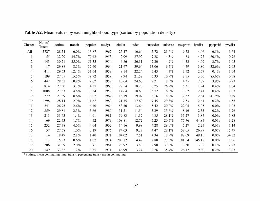
Table A2. Mean values by each neighborhood type (sorted by population density)

Cluster No. of Tracts cotime transit popden medyr cbdist stden intsctden culdesac rswprdist bprdist ppoprsbf hwydist

All 5727 28.54 6.0% 13.87 1967 25.47 16.64 5.72 21.6% 9.72 4.06 6.5% 1.641 55 32.29 34.7% 79.42 1953 2.99 27.92 7.28 4.3% 4.83 4.77 80.5% 0.782

5.43

143 30.71 25.0% 51.35 1954 6.86 26.11 7.20 4.9% 4.52 4.09 3.7% 1.053 17 29.88 8.5% 32.60 1964 21.97 39.64 13.06 6.5% 4.59 3.80 32.6% 2.034 414 29.63 12.4% 31.64 1958 9.14 22.24 4.3% 3.52 2.57 0.4% 1.045 199 27.55 15.5% 19.72 1959 9.94 21.52 6.33 10.9% 2.55 3.36 85.6% 0.586 447 28.31 10.8% 19.62 1952 10.64 24.60 7.21 8.3% 4.35 2.87 3.9% 0.937 814 27.50 3.7% 14.37 1968 27.54 18.20 6.25 26.9% 5.31 1.94 0.4% 1.048 1008 27.33 4.8% 13.34 1959 14.64 18.63 5.72 16.3% 3.62 2.41 0.4% 1.039 279 27.69 8.6% 13.02 1962 18.19 19.07 6.16 16.9% 2.32 2.64 41.9% 0.69

10 298 28.14 2.9% 11.67 1980 21.75 17.60 7.45 29.3% 7.53 2.61 0.2% 1.5511 241 26.75 2.6% 6.40 1964 53.30 13.64 5.42 20.0% 22.05 5.05 0.0% 1.0512 859 29.81 2.3% 5.66 1980 31.21 11.54 5.39 33.6% 8.16 2.33 0.2% 1.7613 213 31.63 1.4% 4.91 1981 59.83 11.12 4.85 28.1% 35.27 3.87 0.0% 1.8314 69 22.73 1.7% 4.52 1979 108.81 12.72 5.23 20.5% 77.76 44.85 0.0% 3.2815 232 27.78 4.6% 4.04 1962 14.16 9.98 4.28 29.0% 5.27 2.25 0.6% 1.1416 57 27.68 1.0% 3.19 1976 84.03 9.27 4.47 28.1% 58.05 26.97 0.0% 15.4917 14 18.49 2.1% 1.40 1971 104.02 7.51 4.34 18.9% 82.09 49.15 0.0% 34.3218 13 15.93 0.6% 1.02 1974 209.12 4.42 2.80 27.0% 181.54 145.18 0.0% 8.0619 206 31.69 2.0% 0.71 1981 28.92 3.80 2.90 37.8% 13.30 3.08 0.1% 2.2320 149 33.32 1.2% 0.35 1971 46.99 3.24 2.26 35.4% 26.12 9.30 0.2% 7.23

* cotime: mean commuting time; transit: percentage transit use in commuting.

32

Table A3. Ranks of neighborhood types by each different variable

NAME FREQPopden

(densest = 1) Stden

(densest = 1) Medyr

(oldest = 1) Cbdist

(shortest = 1) Rswprdist

(shortest = 1) Average rank Average rank Average rank Average rank Average rank

type1 55 79.42 1 27.92 2 1953 2 2.99 1 4.83 8type2 143 51.35 2 26.11 3 1954 3 6.86 2 4.52 6type3 17 32.60 3 39.64 1 1964 9 21.97 10 4.59 7type4 414 31.64 4 22.24 5 1958 4 9.14 3 3.52 3type5 199 19.72 5 21.52 6 1959 5 9.94 4 2.55 2type6 447 19.62 6 24.60 4 1952 1 10.64 5 4.35 5type7 814 14.37 7 18.20 9 1968 11 27.54 11 5.31 10type8 1008 13.34 8 18.63 8 1959 6 14.64 7 3.62 4type9 279 13.02 9 19.07 7 1962 7 18.19 8 2.32 1

type10 298 11.67 10 17.60 10 1980 17 21.75 9 7.53 11type11 241 6.40 11 13.64 11 1964 10 53.30 15 22.05 14type12 859 5.66 12 11.54 13 1980 18 31.21 13 8.16 12type13 213 4.91 13 11.12 14 1981 19 59.83 16 35.27 16type14 69 4.52 14 12.72 12 1979 16 108.81 19 77.76 18type15 232 4.04 15 9.98 15 1962 8 14.16 6 5.27 9type16 57 3.19 16 9.27 16 1976 15 84.03 17 58.05 17type17 14 1.40 17 7.51 17 1971 12 104.02 18 82.09 19type18 13 1.02 18 4.42 18 1974 14 209.12 20 181.54 20type19 206 0.71 19 3.80 19 1981 20 28.92 12 13.30 13type20 149 0.35 20 3.24 20 1971 13 46.99 14 26.12 15

All 5727 13.87 16.64 1967 25.47 9.72

33

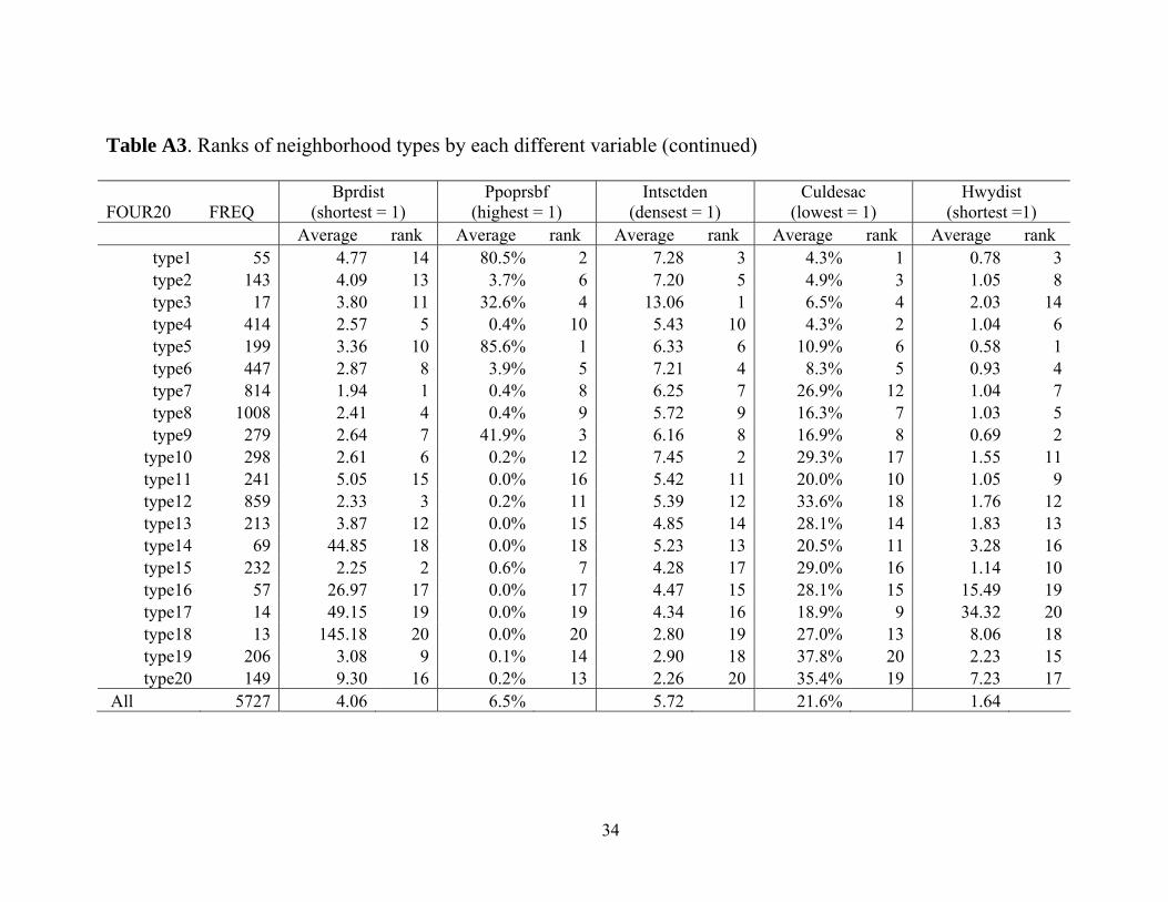
Table A3. Ranks of neighborhood types by each different variable (continued)

FOUR20 FREQBprdist

(shortest = 1) Ppoprsbf

(highest = 1) Intsctden

(densest = 1) Culdesac

(lowest = 1) Hwydist

(shortest =1) Average rank Average rank Average rank Average rank Average ranktype1 55 4.77 14 80.5% 2 7.28 3 4.3% 1 0.78 3type2 143 4.09 13 3.7% 6 7.20 5 4.9% 3 1.05 8type3 17 3.80 11 32.6% 4 13.06 1 6.5% 4 2.03 14type4 414 2.57 5 0.4% 10 5.43 10 4.3% 2 1.04 6type5 199 3.36 10 85.6% 1 6.33 6 10.9% 6 0.58 1type6 447 2.87 8 3.9% 5 7.21 4 8.3% 5 0.93 4type7 814 1.94 1 0.4% 8 6.25 7 26.9% 12 1.04 7type8 1008 2.41 4 0.4% 9 5.72 9 16.3% 7 1.03 5type9 279 2.64 7 41.9% 3 6.16 8 16.9% 8 0.69 2

type10 298 2.61 6 0.2% 12 7.45 2 29.3% 17 1.55 11type11 241 5.05 15 0.0% 16 5.42 11 20.0% 10 1.05 9type12 859 2.33 3 0.2% 11 5.39 12 33.6% 18 1.76 12type13 213 3.87 12 0.0% 15 4.85 14 28.1% 14 1.83 13type14 69 44.85 18 0.0% 18 5.23 13 20.5% 11 3.28 16type15 232 2.25 2 0.6% 7 4.28 17 29.0% 16 1.14 10type16 57 26.97 17 0.0% 17 4.47 15 28.1% 15 15.49 19type17 14 49.15 19 0.0% 19 4.34 16 18.9% 9 34.32 20type18 13 145.18 20 0.0% 20 2.80 19 27.0% 13 8.06 18type19 206 3.08 9 0.1% 14 2.90 18 37.8% 20 2.23 15type20 149 9.30 16 0.2% 13 2.26 20 35.4% 19 7.23 17

All 5727 4.06 6.5% 5.72 21.6% 1.64

34

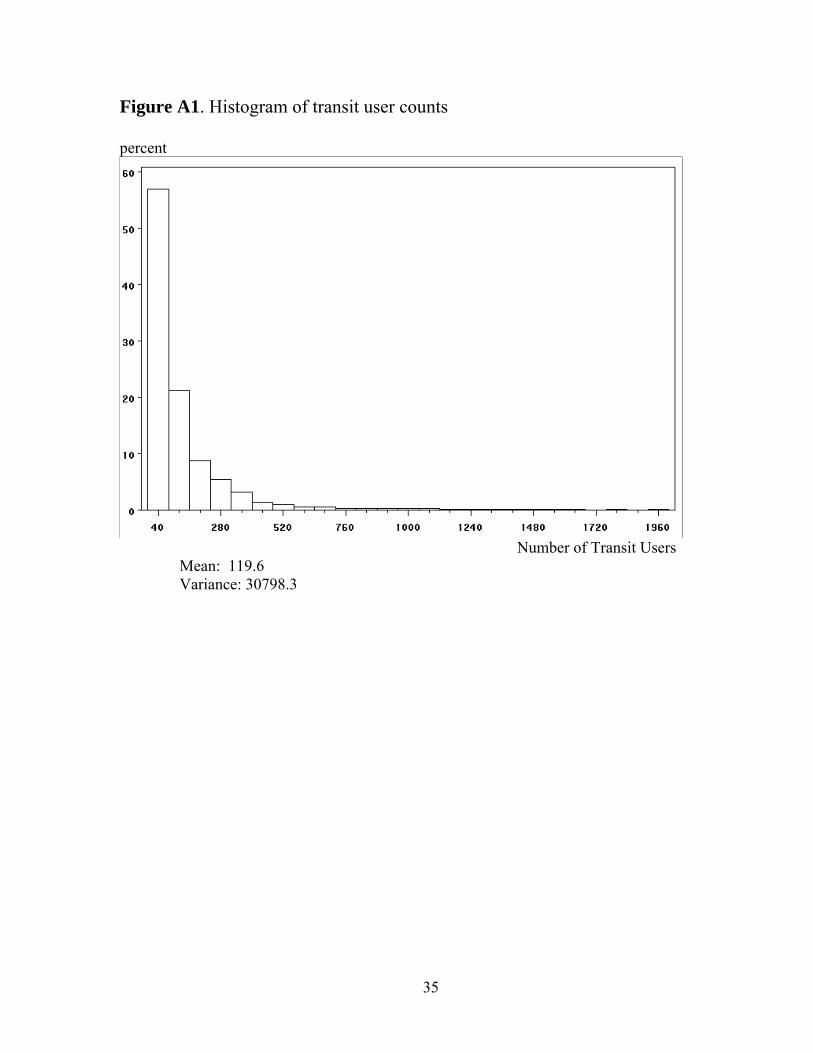
Figure A1. Histogram of transit user counts

percent

Number of Transit Users Mean: 119.6 Variance: 30798.3

35

Residence Types1234567891011121314151617181920

La_hwy.shp

20 0 20 40 Miles

Residential Neighborhood types

Figure A2-a. Geographical clustering of neighborhood types in Los Angeles

36

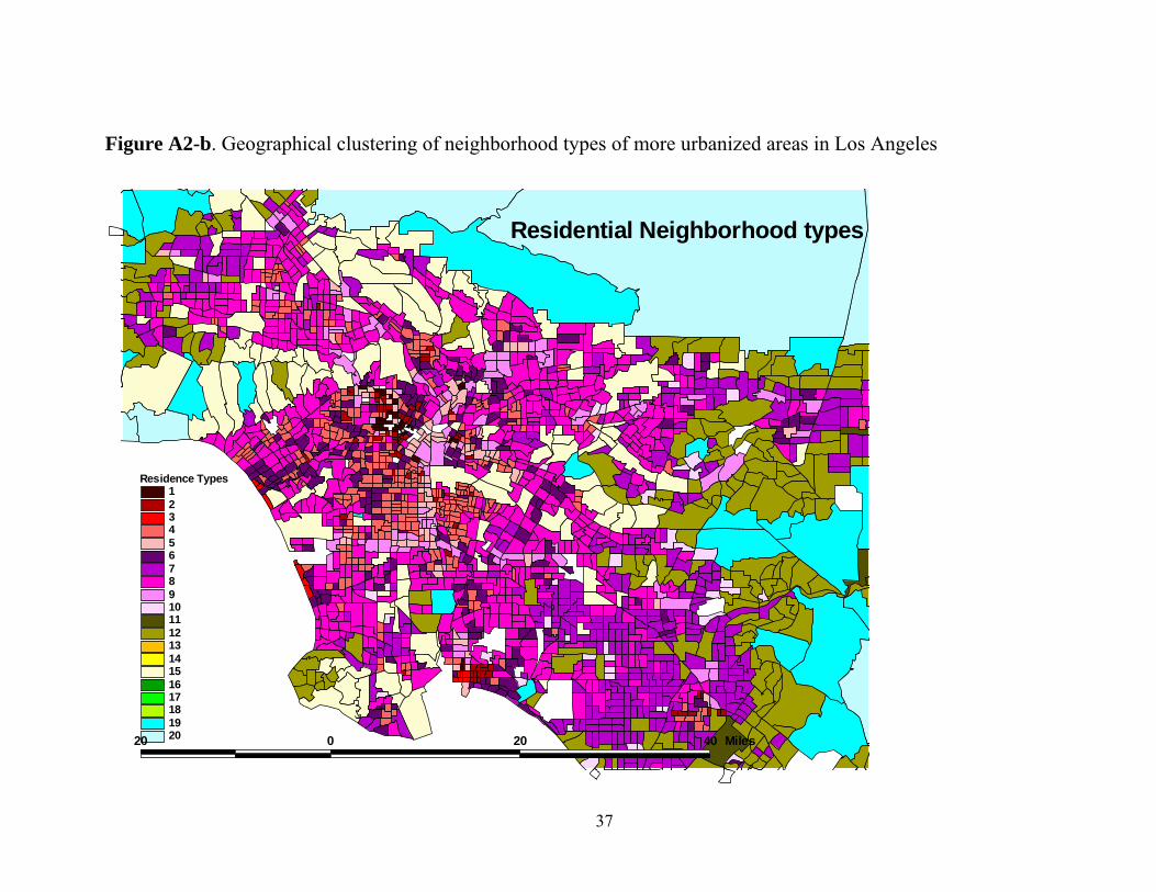
Figure A2-b. Geographical clustering of neighborhood types of more urbanized areas in Los Angeles

Residence Types123456789101112131415161718192020 0 20 40 Miles

Residential Neighborhood types

37