NBER WORKING PAPER SERIES

CONSUMPTION VS. EXPENDITURE

Mark AguiarErik Hurst

Working Paper 10307http://www.nber.org/papers/w10307

NATIONAL BUREAU OF ECONOMIC RESEARCH1050 Massachusetts Avenue

Cambridge, MA 02138February 2004

We would like to thank Fernando Alvarez, Marianne Bertrand, Ricardo Caballero, Steve Davis, Steve Haider,Lars Hansen, Mike Hurd, Anil Kayshap, Helen Levy, Anna Lusardi, Chris Mayer, Amil Petrin, Karl Scholz,Jon Skinner, Mel Stephens, and Steve Zeldes, along with seminar participants at MIT, University of Chicago,University of Wisconsin, Columbia University, and RAND, for their helpful comments. We are extremelygrateful of Bin Li for her exceptional research assistance. Both Aguiar and Hurst would like to acknowledgethe financial support of the University of Chicago's Graduate School of Business. The views expressed hereinare those of the authors and not necessarily those of the National Bureau of Economic Research.

©2004 by Mark Aguiar and Erik Hurst. All rights reserved. Short sections of text, not to exceed twoparagraphs, may be quoted without explicit permission provided that full credit, including © notice, is givento the source.

Consumption vs. ExpenditureMark Aguiar and Erik HurstNBER Working Paper No. 10307February 2004JEL No. E2, J1, J2

ABSTRACT

Standard tests of the permanent income hypothesis (PIH) using data on nondurables typically equate

expenditures with consumption. However, as noted by Becker (1965), consumption is the output of

a "home production" function that uses both expenditure and time as inputs. With this in mind, we

revisit the retirement consumption puzzle by documenting that the dramatic decline in expenditures

at the time of retirement is matched by an equally dramatic rise in time spent on home production.

The innovation of our paper is that we empirically disentangle changes in actual consumption from

changes in expenditures. To do so, we use a novel data set which collects detailed food diaries for

a large cross-section of U.S. households. We show that despite the decline in food expenditures,

neither the quantity nor the quality of food intake deteriorates with retirement status. However,

unemployed households experience a decline in consumption commensurate to the impact of job

displacement on permanent income. Taken together, the results on retirement and unemployment

highlight how direct measures of consumption distinguish between anticipated and unanticipated

shocks to income, while using expenditure alone obscures this difference and leads to false

rejections of the PIH.

Mark AguiarUniversity of ChicagoGraduate School of Business Chicago, IL 60637mark.aguiar@gsb.uchicago.edu

Erik HurstGraduate School of BusinessUniversity of Chicago213A Walker MuseumChicago, IL 60637and NBERerik.hurst@gsb.uchicago.edu

1

I. Introduction

Standard tests of the permanent income hypothesis (PIH) using data on nondurables typically

equate consumption with expenditure.1 However, as noted by Becker (1965), consumption is the output

of “home production” which uses as inputs both market expenditures and time.2 To the extent possible,

individuals will substitute away from market expenditures towards time spent in home production,

including more intensive search for bargains, as the relative price of time falls. In this sense, an

individual’s opportunity cost of time has a direct bearing on the total cost of consumption, making market

expenditures a poor proxy for actual consumption. In particular, consumption may remain constant even

while observed market expenditures fluctuate.

In this paper, we directly examine the link between expenditures, time spent on home production,

and actual consumption. To do this, we exploit a novel dataset - the Continuing Survey of Food Intake of

Individuals (CSFII), conducted by the U.S. Department of Agriculture – which tracks the dollar value, the

quantity, and the quality of food consumed within U.S. households. These data allow us to distinguish

empirically between food expenditure and food consumption. We find that agents, in response to

forecastable income changes, smooth consumption, but not necessarily expenditures, as predicted by the

standard PIH model augmented with search/home production.

We use this data to revisit two major stylized facts in the household consumption literature:

household non-durable consumption drops significantly during retirement (Banks, Blundell, and Tanner

(1998), Bernheim, Skinner, and Weinberg (2001), Haider and Stephens (2003)) and household non-

durable consumption drops significantly during unemployment (Stephens (2001)). The majority of

researchers documenting these stylized facts use food expenditures as their measure of non-durable

consumption. Some authors have interpreted the decline in expenditure at the onset of retirement as being 1 This literature is vast. See surveys by Browning and Lusardi (1996) and Attanasio (1999). We use the terms Permanent Income Hypothesis, Life-cycle Model, and “consumption smoothing” to refer to the class of models in which agents seek a constant marginal utility of consumption (up to an adjustment for differences between time preference and the interest rate). 2 See also Ghez and Becker (1975). Becker’s insight was revived and extended by, among others, Benhabib, Rogerson, and Wright (1991), Greenwood and Hercovitz (1991), Rios-Rull (1993), and Baxter and Jermann (1999). Rupert, Rogerson and Wright (1995, 2000) and McGrattan, Rogerson, and Wright (1997) provide empirical evidence documenting the importance of home production.

2

evidence that households do not plan sufficiently for retirement (Bernheim et. al. (2001)), while others

conclude that there is some unexpected news about lifetime resources that occurs at the time of retirement

(Banks et al (1998)). Angeletos et al. (2001) interpret decline in expenditure at the time of retirement as

evidence that household preferences are time inconsistent. Using the CSFII data, we find that

consumption expenditures fall by 17% at retirement.3 However, this decline is accompanied by a 53%

increase in time spent in home production (shopping for and preparing food) by individuals during

retirement.

Given the sharp increase in time spent shopping for and preparing food, the pattern for expenditures

may differ significantly from the pattern of actual consumption. To explore the response of consumption

during retirement, we perform a comprehensive analysis of individual food diaries of retirement-age

household heads. We first document that nutritional summary statistics of individual diets do not vary by

retirement status. These nutritional measures include calories, vitamin content, protein, fat, cholesterol,

and calcium. While rough aggregates, many of these measures (particularly cholesterol, fat, and

vitamins) display strong income elasticities across working-age employed households, yet do not vary at

all with retirement status. Secondly, we identify several individual food categories that display large

income elasticities. For example, high income households tend to eat more fresh fruit, shellfish and wine,

and less hot dogs and ground beef. Again, we find the frequency which retirees consume any of the

individual food categories is essentially identical to nonretirees with similar demographics. Thirdly, we

examine consumption categories within which we can identify an observable quality component. For

example, while retirees are less likely to eat out, the difference comes almost exclusively from a decline

in visits to fast food restaurants. We find, however, that the probability of dining at a restaurant with table

service does not vary across retirement status. If the individual was ill-prepared for retirement, we would

expect them to switch to lower quality goods. However, we find that retirees are just as likely to consume

brand name products (as oppose to generic store brands) and that they do not switch towards fattier cuts

of meat (as oppose to lean cuts of meat). 3 Bernheim et. al. (2001) find similar food expenditure declines upon retirement in a sample of PSID households.

3

While the fact that numerous individual components of consumption do not change during

retirement is very informative, the CSFII data contains thousands of consumption categories. We

therefore conduct a systematic analysis of the entire consumption basket of households. To do this, we

first show that a standard intertemporal model of consumption, augmented to allow for home production,

implies a one-to-one mapping from the entire vector of consumption categories along with total

expenditure of the consumption basket, to the marginal utility of wealth (or the multiplier on lifetime

resources). Taking this relationship to the data is complicated by the fact that agents face different

relative prices depending on the opportunity cost of time. We show that this can be accommodated in a

large class of home production models by including total expenditure as an additional control. Using a

large number of consumption goods, we then estimate this mapping and test whether retirees experience a

significant change in marginal utility. This is a direct test of the PIH given that retirement is an

anticipated change in current income. Using several alternative sub-samples and specifications, we find

no evidence that marginal utility changes with retirement status. Additionally, we are able to create a

theoretically based composite consumption index. As seen in Figure 1, our composite consumption index

is essentially flat across retirement ages despite the dramatic fall in expenditure.

We perform the same battery of tests to determine whether unemployment results in a consumption

decline. As with retirement, the unemployed experience a decline in expenditures in both food at home

and food away from home, with total expenditure falling 19%. The unemployed increase time spent in

home production as well, although to a lesser extent than the retirees. In sharp contrast to retirement,

however, our formal test of the PIH indicates that unemployment results in a significant decline in

consumption. Controlling for demographics, our composite consumption index for unemployed

households suggests a 5 to 6% decline in lifetime resources. This is not surprising given that other

researchers have documented that involuntary job loss results in a persistent decline in annual income of

roughly 8-10%.4 The results on unemployment are therefore consistent with the PIH in the absence of

perfect social insurance and provide an interesting counterpoint to retirement. That is, direct observation 4 See Huff-Stevens (1997).

4

of consumption indicates a quantifiable difference between an unanticipated shock to permanent income

and an anticipated shock such as retirement. This difference is obscured when one looks solely at

expenditure.

This paper breaks new ground by looking directly at the home production function for food. Food

expenditure has been used extensively in the estimation of consumption Euler equations using micro data

sets (see surveys by Browning and Lusardi (1996) and Attanasio (1999)). The reason for the prominent

use of food consumption is two fold. First, panel data sets, primarily the Panel Study of Income

Dynamics (PSID), report only food expenditures out of the class of nondurable goods. Secondly, food is

a necessary good with a small income elasticity, making it a strong test for consumption smoothing.

However, as we show in this paper, the elasticity of substitution between time and expenditures may be

large in the production of food intake; one can spend less money at the market and more time shopping or

in the kitchen to produce an equivalent quantity of food. Given home production, we conclude that

certain expenditures, particularly expenditures on food, are poor proxies for actual household

consumption and mask the extent to which individuals smooth consumption in practice. However, it

should be noted that search can reduce the expenditure of all goods, not just expenditures on food, if

prices vary across retail outlets. To this end, we show that time spent shopping for non-food household

items increase by 60% at the time of retirement.

The rest of the paper is organized as follows: Section 2 describes the two data sets used in the

paper; Section 3 explores expenditure and time use in retirement; Section 4 studies the response of

individual measures of consumption; Section 5 presents a formal model that allows a systematic test of

the PIH using a full vector of consumption and expenditure data; Section 6 studies expenditure, time use

and consumption during unemployment; and Section 7 concludes.

II. Data

For our primary analysis, we use data from the Continuing Survey of Food Intakes by Individuals

(CSFII) collected by the U.S. Department of Agriculture. Since the 1930's, the U.S. Department of

5

Agriculture has conducted nationwide food surveys in order to monitor the health and dietary habits of the

U.S. population. The survey is cross sectional in design and is administered at the household level. We

make use of the two most recent cross sectional surveys; the first interviewed households between 1989

and 1991 (CSFII_89) and the second interviewed households between 1994 and 1996 (CSFII_94).

Despite presenting a unique opportunity to study household consumption patterns, the CSFII data sets

have been relatively unexploited by economists.5

The CSFII_89 included two independent random samples of the U.S. population. The "main"

sample was designed to be nationally representative of all U.S. households. The "low-income" sample

was designed to over-sample the poor by limiting eligibility to households with gross income for the

previous month at or below 130 percent of the Federal poverty threshold. Unless we are specifically

looking at a sample of low income households, we restrict all of our analysis to the main sample. The

CSFII_94 was designed to obtain a nationally representative sample of non-institutionalized persons

residing in households within the United States. The CSFII_94 differed slightly in design from the

CSFII_89 in that it did not over-sample the poor.6 All individuals within the households in both CSFII

cross sections were asked to complete the survey. When analyzing individual-level data, we restrict our

analysis to only include household heads. If more than one person in the household identified themselves

as being the household head, we selected only the male member to maintain consistency with alternative

household datasets, such as the Panel Study of Income Dynamics (PSID). The CSFII_89 interviewed

15,192 individuals in 6,718 distinct households while the CSFII_94 interviewed 16,103 individuals in

8,067 distinct households. The response rates for both surveys were high (over 85%). For all the analysis

below, we pool the CSFII_89 and the CSFII_94 datasets.

The data sets track standard economic and demographic characteristics of its survey respondents

including age, educational attainment, race, gender, occupation, employment status, hours worked,

retirement status, family composition, geographic census region, whether the household lives in an urban

5 See Wilde and Ranney (2000) and Shapiro (2003) for exceptions. Both papers examine the food intake of welfare recipients. 6 See the Data Appendix for a detailed discussion of the sampling techniques used in the CSFII_89 and the CSFII_94.

6

area and household income. Additionally, given the Department of Agricultures goals, the survey asks

respondents detailed health questions. These health questions come in three forms. First, respondents are

asked to self assess their own health as being either excellent, very good, good, fair or poor. Such a

question is similar to health questions asked in the PSID and the Health and Retirement Survey (HRS).

Second, the respondents are asked specific health questions such as "Do you have high blood pressure?",

"Do you have cancer?", "Have you had a stroke?", etc. We summarize all such questions regarding the

household head's health inventory in the Data Appendix. Lastly, survey respondents are asked specific

physiological questions such as height and weight.

The CSFII data sets also track two separate measures of consumptions. First, like the PSID and the

HRS, respondents are asked to report their total expenditure during the previous month for food

purchased at the grocery store, food delivered into the home, and food purchased at restaurants, bars,

cafeterias or fast food establishments. We refer to the former two food expenditure measures as food

expenditures “at home” while the latter measures food expenditures “away from home”. This

classification provides consistency with the food expenditure questions from the PSID.

As we discussed above, food expenditure need not reflect actual food intake due to home

production. The CSFSII data allows a different – and arguably better – measure of food consumption.

Each household in the CSFII data fill out detailed food diaries which are designed to record their total

food intake during a given 24 hour period. The data is collected in person by a trained CSFII interviewer.

The interviewer began by asking the sample person to report everything eaten or drunk the previous day

between midnight and midnight.7 The CSFII_89 collected detailed food diaries on three days while he

CSFII_94 collected detailed food diaries on two non-consecutive days. All data was collected via an in-

home visit by a trained CSFII interviewer. The Data Appendix discusses the methodology of the food

7 The interviewers were not allowed to interrupt the respondent (sample person) during this initial listing of the day's intake. The sample person was invited to add any other items remembered as the interview progressed. Then, for each food and drink mentioned by the respondent, the CSFII interviewer followed up with detailed questions about that food item to illicit more information (i.e., the brand name, was it reduced calorie, was it high fiber, what type of fat or oil was used in preparing the meal, etc.). Additionally, the interviewer was armed with measuring cups, rulers, and graphical aides to help the respondent report accurate quantities. We found no evidence that the quality of responses differed between retired and non-retired households. See the "Documentation to the 1994-1996 Continuing Survey of Food Intakes by Individuals" for complete survey methodology.

7

diary in much greater detail. In the empirical work that follows, we average each of our daily food intake

measures over all the days for which the individual completed the food diary (i.e., over three days for the

CSFII_89 and over two days for the CSFII_94).

Lastly, the CSFII data sets have measures of household income and wealth. The surveys report

total labor income and income from interest and dividends for the household over the last year. The

surveys also report the previous month’s income from wages or salary for the household and the usual

hours worked per week for the household head. Both surveys ask whether the household owns their own

home. Additionally, the households are asked whether they have over $5,000 in "Cash, savings or

checking accounts, stocks, bonds, mutual funds, and certificates of deposits". If the respondent answers

no, they were asked to provide the amount of liquid assets they had less than $5,000.

Appendix Table A1 shows that a sample of household heads between the ages of 22 and 65 from

the CSFII datasets mirrors a similarly defined sample from the 1993 PSID. Specifically, the proportion of

heads that are male (75% vs 74%), the percent that are black (13% vs 14%), the percent with only a high

school degree (35% vs 36%), the percent that own homes (60% for both), the percent employed (75% vs

81%), and the percent retired (7% vs. 6%) are nearly identical between the CSFII data sets and the 1993

PSID. More importantly, the average yearly household total food expenditure in the CSFII ($5,600/year,

in 1996 dollars) is essentially the same as the average yearly household total food expenditure in the PSID

($5,400/year, in 1996 dollars). Likewise, the propensity for households to report themselves as being in

good health or better is similar between the two surveys (85% in the CSFII vs 88% in the PSID). The

Data Appendix discusses more fully how the CSFII data matches up with the PSID. In particular, the

results from Appendix Table A1 document that the CSFII data is of good quality and representative of the

U.S. population.

Aside from a question regarding shopping frequency, the CSFII data does not explicitly track time

spent on home production. To examine the extent to which households spend time in food production, we

make use of an additional data set: the National Human Activity Pattern Survey (NHAPS) conducted for

the United States Environmental Protection Agency by the Survey Research Center at the University of

8

Maryland and administered between the fall of 1994 and the fall of 1996. The survey was designed to

provide estimates of potential exposure to pollutants in air, water, and soil systems with which people in

the United States come into contact throughout their typical daily routine. The study was a random-digit

telephone survey of households in the continental U.S. Only one individual per household was included

in the survey. The survey respondent in each household was chosen randomly (including children) based

on which household member would have the next birthday. The total sample included 9,386

individuals.8

As part of the survey, each respondent was asked to provide a minute-by-minute time diary of the

previous 24 hour day. The survey administrators at the University of Maryland aggregated up the

information from the time diaries into 91 time use categories.9 In this paper, we use two of these

aggregate time use categories: "minutes spent preparing food" and "minutes spent shopping for food".

In additional to the time diaries, the NHAPS asked the respondent to provide background information.

While this information is far less extensive than in the CFSII data, it does include: age, gender, race,

educational status, Census region, current work status, whether the individual is retired, whether the

individual is unemployed, the size of the household to which the individual belongs, and whether the

individual is a homeowner or renter. The data does not explicitly ask questions about the individual's

income or wealth.

III. Expenditure and Time Use among the Retired

Retirement, for most households, is a discreet, planned event (Haider and Stephens (2003)).

According to the permanent income hypothesis, forward looking agents will smooth their marginal utility

of consumption across predictable income changes. However, there is a large literature which documents

8 While many other surveys ask detailed information on individual time use (i.e., Michigan Time Use Survey, The American's Use of Time, and the Time Use Longitudinal Panel), the NHAPS data set has two advantages. The first, and most important, is the large sample size. Neither the Michigan Time Use Survey nor the Time Use Longitudinal Panel has sample sizes exceeding 2,000 individuals. Additionally, the NHAPS data surveys households in recent time periods unlike the Michigan Time Use Survey (1965 and 1975), the American's Use of Time (1965-1966) or the Time Use Longitudinal Panel (1975, 1976, and 1981). Starting in 2003, the U.S. Census, via the Current Population Survey, will ask detailed questions about individual time use. This data is not expected to be available to researechers until late 2004. 9 See EPA report EPA/600/R-96/148 (July 1996) for a detailed description of the survey methodology and coding classifications.

9

that upon retirement, household expenditures fall dramatically (Banks, Blundell, and Tanner (1998),

Bernheim, Skinner and Weinberg (2001), Miniaci, Monfardini and Weber (2002), Haider and Stephens

(2003), and Hurd and Rohwedder (2003)). The literature refers to such a finding as “the retirement

consumption puzzle”. Specifically, using PSID data, Bernheim et. al. (2001) find that: 1) total food

expenditure declines by about 30% between the pre and post retirement periods for the average

household, 2) the decline in expenditure occurs for both food purchased at grocery stores and food “away

from home”, and 3) total expenditures decline dramatically regardless of the household's position in the

pre-retirement wealth distribution. With respect to the last point, they find that households with pre-

retirement wealth in the lowest wealth quartile experience a 57% decline in expenditure during the

subsequent two years after retirement. The comparable decline in expenditure for households in the

second wealth quartile, third wealth quartile, and the top wealth quartile are 29%, 30%, and 21%,

respectively.10 They find that while the decline in expenditure is largest among low wealth households,

very wealthy households and median wealth households experience similar declines in food expenditure

at the time of retirement.

The decline in expenditures at the time of retirement is not limited to food. Banks, Blundell and

Tanner (1988) use the British Family Expenditure Survey to document that total expenditures decline

sharply at the incidence of retirement.11 Some authors have interpreted the decline in expenditure at the

onset of retirement as being evidence that households do not plan sufficiently for retirement (Bernheim et.

al. (2001)), while others conclude that there is some unexpected news about lifetime resources that occurs

at the time of retirement (Banks et al (1998)). Angeletos et al. (2001) interpret decline in expenditure at

the time of retirement as evidence that household preferences are time inconsistent.12

10 Table 3 and Figure 4 of Bernheim, Skinner and Weinberg (2001). 11 Miniaci, Monfardini and Weber (2002), using Italian data, also find evidence of large total expenditure declines at the time of retirement. 12 Hurd and Rohwedder (2003) exploit expectation questions in the HRS to illustrate that most households expect a decline in consumption expenditures during retirement. They conclude that the decline in consumption expenditures at the time of retirement does not result from poor planning on the part of the household. Additionally, they report survey evidence from the HRS that time spent on home production increases after retirement. Our paper complements their work by examining the change in actual consumption intake that occurs as a household retires.

10

In this and the subsequent two sections, we use the CSFII and NHAPS data sets to illustrate that the

retirement consumption puzzle is no puzzle at all once we disentangle consumption from expenditure.

Given that their opportunity cost of time has declined, retired individuals will be more willing to expend

effort to reduce the market prices they face for a given unit of consumption. When time is cheap,

individuals are likely to substitute toward time intensive activities like clipping coupons, searching for

sales across multiple stores, or engaging in home production. All of which will reduce the price paid by

those individuals for a given unit of consumption. With respect to food expenditure in particular, home

production is very important. An individual can spend less by making a meal from scratch as opposed to

ordering that same meal from a take-out restaurant or the grocer’s deli section. If time can be used to

reduce market costs, one would expect expenditure on food to fall and time spent on food production

(shopping for food and preparing meals) to rise as households enter retirement. Actual consumption may

not change despite the decline in expenditure.

To examine food expenditure, time spent on food production, and food consumption at the onset of

retirement, we restrict both the CSFII and NHAPS samples to include only households with heads

between the ages of 57 and 71 for which there is a full set of control variables (2,052 household heads and

1,308 individuals for the CSFII and NHAPS samples, respectively). The vast majority of households

retire between 57 and 71. Less than 10% of the CSFII household heads are retired prior to the age of 57

and over 70% are retired by the age of 71. This number is similar to retirement propensities in the Health

and Retirement Survey (HRS).

To begin, we document the “retirement consumption puzzle” using expenditure from the CSFII

data sets. Figure 1 plots the average total expenditure on food for male household heads aged 57 - 71, by

three year age ranges.13 As retirement propensities increase with age, household expenditure declines

sharply with age. The peak retirement age range for individuals is 63-65. Over 50% of all household

13 In Figure 1, we focus on only male household heads. We do this because the probability that a female is a household head increases with age (given differences in mortality rates across the sexes). Given that females eat less than males, we may observe consumption falling with age simply as a result of differences in sample composition. In all our regression work below, we focus on the full sample of household heads and include controls to account for changes in sample composition.

11

heads retire within this age range. Between 60-62 (pre-peak retirement age) and 66-68 (post-peak

retirement age), household expenditure on food declines by 13% for male headed households (p-value

<0.01). Notice, prior to age 62, expenditure is constant. Figure 2 decomposes expenditure for all

households (both male and female headed) in the CSFII sub-sample by retirement status. Households

with a retired head spend 11% less on food than their non-retired counterparts ($377 vs. $423, p-value of

difference <0.01).

The decline in consumption expenditures with age or at the time of retirement is robust to the

inclusion of a rich set of controls designed to capture changing demographics and health among older

households. The top portion of Table 1 reports the estimates to the following two regressions:

0 1 2ln( )it it it itx Retired Z uα α α= + + + (3.1) 0 1 2ln( ) _ 63it it it itx Age Z vβ β β= + + + (3.2)

where xit is total food expenditure, expenditures on food “at home”, or expenditures on food “away from

home”, depending on the specification, for household i in year t. Retiredit is a dummy variable equal to 1

if the household head i is retired in year t, Age_63it is a dummy variable equal to 1 if household head i is

63 years old or older in year t, and Zit is the vector of year, region, demographic and health controls.

Specifically, the Z vector includes a series of controls for household composition including family size,

education dummies for the household head, a dummy variable equal to 1 if the household head is black, a

dummy variable equal to 1 if the household head is male, dummies indicating census regions, and time

dummies. The Z vector also includes all the health controls discussed in the Data Appendix.

Given that the timing of retirement can also be correlated with unmeasured variables which affect

the household's expenditure decisions, we estimate (3.1) via an instrumental variable procedure. As is

common in the literature, we use age as our instrument for retirement.14 Age naturally has strong

14 At a mechanical level, the research design we implement throughout this paper, via instrumenting for retirement status with age, compares the behavior households in their early 60s, where there is less than 20% of household heads retired, to households aged in their mid 60s, where over 70% of household heads are retired. The difference in sample composition from comparing essentially 62 year olds to essentially 66 year olds is small. According to the 1989-1991 U.S. Census Mortality Tables, the

12

predictive power for the household head's retirement status. The adjusted R-squared of a regression of

household retirement status on age controls is 0.19 (with an associated F-statistic of 119.0).15 The top

rows of Table 1 report that even after controlling for year, region, demographic and health controls,

retired households spend 17% less on total food (p-value <0.01 ), 15% less on food at home (p-value =

0.01), and 31% less on food away from home (p-value = 0.01). The results are broadly consistent with

the findings of Bernheim et al. (2001) and Haider and Stephens (2003).16 For robustness, we estimate

equation (3.2) via OLS with the variable of interest being a dummy variable indicating whether the

household head is aged 63 or older. The results, reported in the second column of Table 1, yield

qualitatively similar conclusions as the IV regressions reported in column I.

While expenditure declines with retirement status, time spent on food production dramatically

increases with retirement status, where we define food production as shopping for food and preparing

meals. Figure 1 shows that male household heads aged 66-68 (post peak retirement years) spend 21%

more time on food production than households aged 60-62 (pre-peak retirement years).17 The pattern

persists when directly comparing retired to non-retired households (Figure 2). Focusing on the NHAPS

sub-sample of individuals aged 57-71, retired individuals spend 27% more time on food production than

their non retired counterparts (47 minutes vs. 37 minutes, p-value of difference <0.01).

While women are more likely than men to engage in home production of food in any period, the

increase in time spent on food production at retirement is most prominent for men. Retired female

household heads spend 17% (51 vs. 60 minutes, p-value = 0.04) more time on food production than their

mortality rates for 62 year olds, 66 year olds, and 68 year olds, are, respectively, 1.4%, 2.0%, and 2.3%. Additionally, the differences in health status between retired and non-retired 57-71 year olds are also minimal. We document this in Appendix Table A2. 15 Haider and Stephens (2003) argue that self-reported retirement expectation is a better instrument for the timing of retirement than age. Using self-reported retirement status as their instrument, they still find that expenditure declines by 8-10% at the time of retirement. In the CSFII data, we only observe a cross section of households and retirement expectations are not asked. 16 The difference between our finding of about a 17% decline in expenditure for the average retired household and Bernheim et al. (2001)’s finding of about a 30% decline in expenditure for the average household is likely due to their using panel data and our using repeated cross sections. 17 Households aged 54-56 (not shown on Figure 1) spend slightly more time on food production than households aged 57-59 (36 minutes/day vs. 34 minutes/day). The amount of time spent on food production by 54-56 year olds is essentially the same as the amount of time spent on food production by 60-62 year olds. The dramatic increase in time spent on food production occurs for households above the age of 62.

13

working counterparts (not reported). Retired men, however, relative to working men, spend 46% more

time on food production (18 vs. 29 minutes, p-value < 0.01).

The bottom rows of Table 1 shows that the effect of retirement on time spent on food production is

even greater once we control for household demographics. Specifically, we estimate the following

regressions:

0 1 2it it it ith Retired Z uα α α= + + + (3.3) 0 1 2_ 63it it it ith Age Z vβ β β= + + + (3.4) where hit measures individual i’s propensity to shop for food or total daily time spent (in minutes) on food

production. The CSFII data asks households whether they do their major shopping at least once a week.

The NHAPS data, as discussed above, records time spent shopping for food and time spent preparing

meals. For the NHAPS data, we also use as a dependent variable a dummy variable indicating whether

time spent on food production is positive, and the log of time spent of food production, conditional on

food production being positive as alternative measures for the dependent variable. Retired, Age_63, and Z

are defined as above.18 In all specifications, we instrument for retirement status using the household

head's age. The adjusted R-squared of a regression of retirement status on age controls in the NHAPS

sub-sample is 0.15 (F-statistic = 67.3).

The lower rows of Table 1 shows that retired households are 17 percentage points more likely to do

their major food shopping on a weekly basis (p-value <0.01). Two thirds of households shop on a weekly

basis implying that retired households are 25% more likely to shop for food at least once per week

(0.16/0.66). Likewise, the NHAPS data shows that retired households spend 18 more minutes per day on

food production (p-value = 0.02) and spend 53% more time on food production, conditional on food

production being positive (p-value <0.01 ). The breakdown between shopping and preparation (not

18 Given that the demographic variables recorded in the NHAPS data are much more limited, the Z vector for time spent on food production include only year, region, sex, household size, education and race controls. The NHAPS dataset does not include any health measures.

14

reported) indicates that retirees spend 42% more time shopping than nonretirees and 54% more time

preparing food, conditional on demographics and positive time spent on the activity.

Our focus thus far has been on food expenditure and food consumption. However, the NHAPS data

also tracks time spent shopping for non-grocery household goods. At the time of retirement, households

increase their propensity to shop for other goods by 50% (0.22 vs 0.16, p-value of difference < 0.01) and

their total time spent shopping for other goods by 64% (23 minutes per day vs. 14 minutes per day, p-

value of difference = 0.01). This suggests that expenditure may not be an accurate measure of actual

consumption for non-food goods. In summary, retired households spend more time shopping for food,

more time preparing food, and more time shopping for other goods compared to their pre-retired

counterparts. Given that both increasing search and increasing home production can reduce prices paid

by households, it is not surprising that expenditure falls during retirement.

It should be noted that 18 minutes a day is a sizeable increase in time spent on food production.

The 18 minutes per day (Table 1) translates into an additional 9 hours per month of food production. If

households value their time during retirement at half the average pre-retirement wage, this would translate

into an additional $81 per month of food production.19 During retirement, total monthly expenditures on

food, conditional on demographics, decline between $70 per month (our data) and $100 per month

(Bernheim et al, 2001). That is, if one values the time of retired households at half their pre-retirement

wage, the increase in time spent in food production for retired households is roughly the same as their

decline in food expenditure.

The fact that time spent on home production increases with retirement status is consistent with the

majority of work which examines time use. For example, Juster and Stafford (1985), in their treatise on

time use, document thoroughly that time spent in home production is negatively correlated with the value

of time. Hurd and Rohwedder (2003) use self-reported data from HRS respondents to document that

retired individuals aged 65-69 spend 100% more time shopping for all goods and 47% more time

19 The average hourly wage of working household heads between the ages of 57 and 71 in the CSFII sample is $18/hour. Half the hourly wage is $9/hour. 9 hours a month of extra food production valued at $9/hour results in an additional $81 per month of food production.

15

preparing meals compared to their non-retired counterparts. Blaylock (1989) finds that shopping

frequency is an increasing function of age among older households. Lastly, Cronovich, Daneshvary, and

Schwer (1997) show that coupon use increases significantly for households older than 65. Taken

collectively, older households by clipping coupons, spending more time on food production, and

shopping more frequently, reduce the price they pay for a given quantity of food consumption. In

summary, previous research and our findings in Figures 1-3 and Table 1 suggest that expenditure is not an

appropriate measure of consumption, especially for retired households were the value of time is changing.

The substantial adjustment in time spent in shopping and home production implies that it is likely

inappropriate to equate expenditure with consumption. In the next two sections, we use better measures

when examining the behavior of consumption in retirement.

IV. Nutrition, Consumption Categories and Luxury Goods in Retirement

As noted above, the CSFII data provide tremendously detailed accounts of an individual’s dietary

habits. To assess whether an individual’s food consumption changes in retirement, we explore the

evidence in four ways. First, we examine the nutritional composition of the individual’s diet. Secondly,

we examine individual categories of food consumption. In both cases, we identify nutritional measures

and consumption categories that exhibit strong income elasticities. This allows us to test whether retirees

switch away from goods preferred by wealthy households. In other words, do retired households behave

as if their permanent income has declined? Thirdly, we explore consumption goods that have an

observable quality component. Specifically, we look at an individual’s propensity to eat out at restaurants

with table service, the individual’s propensity to eat branded foods as oppose to store or generic brands,

and the individual’s propensity to eat lean cuts of meat as oppose to fattier cuts of meat. If an individual

is unprepared for retirement, we would expect that individual to switch towards lower quality goods

(fattier cuts of meat, generic brands) or to switch away from luxury goods (restaurants with table service).

Lastly, in Section V, we conduct a systematic test of the PIH using a formal model and an aggregate of a

much larger set of consumption and expenditure measures.

16

The CSFII reports summary statistics for each individual’s daily diet. This procedure is discussed

in detail in the Data Appendix. We start our analysis by focusing on 8 nutritional measures: total

calories, vitamin A, vitamin C, vitamin E, calcium, saturated fat, cholesterol, and protein. Our

methodology has two components. First, we want to establish that these nutritional measures vary with

lifetime resources. Second, we show whether the amount of these nutritional measures consumed

changes with retirement status.

Table 2 shows the results of the analysis of nutritional measures. The first panel reports the income

elasticity of these nutritional measures for a sample of household heads between the ages of 25 and 55

who are working full time. To obtain this elasticity, we estimate an IV regression of the log of the

nutrition measure on the log of income as well as controls for race, sex, family composition, height and

health controls. We instrument current household income with occupation, education, education and

occupation interactions, and sex and race interactions. In this sense, we only use the “permanent”

component of variation in income. Aside from the log calories regression, all other regressions in panel I

include log calories as an additional control. In the second panel, we regress this same dependent variable

on a dummy variable equal to 1 if the household head is retired (instrumented with age dummies). This

sample is the same used to compute the estimates in Table 1 (i.e., it includes all household heads aged 57

– 71). This regression also includes race, sex, year, region, household composition, and health controls.

As has been documented by others in the literature, log calories do not vary with permanent income

within a cross section of younger, working households (Panel I of Table 2). Specifically, using the CSFII

data, employed household heads with higher income consume similar amounts of calories as employed

household heads with lower income. Even allowing for a more flexible functional form (i.e., including a

cubic in permanent income), log calories does not respond much to changes in permanent income. This

implies that even if an individual is unprepared, we may not expect calories to differ for that individual

prior to and after retirement.

While calories do not vary with the level of permanent income, other dietary components,

conditional on log calories, respond strongly to permanent income. Specifically, the income elasticity of

17

vitamin A and vitamin C are over 0.30 (p-value < 0.01) and the income elasticity of vitamin E and

calcium are 0.17 and 0.08, respectively (p-value of both < 0.01). Likewise, cholesterol and saturated fat

are inferior goods (respectively, income elasticities equal to -0.25 and -0.08, p-value for both < 0.01).

These results are robust to the inclusion of controls for whether the household head is taking specific

vitamin supplements. Furthermore, non-linear estimation (not reported) finds that vitamins (either A, C,

or E) are a strictly increasing function of income over all observed income ranges. Likewise, cholesterol

is a strictly declining function of income over all observed income ranges. The results suggest that

individuals can consume cheap calories by switching their diet towards fat and cholesterol and away from

vitamins and calcium. The finding that “fat” is cheap and “healthy diets” are expensive is consistent with

a large literature on nutrition and income.20

The results from panel I of Table 2 suggest that if an individual enters retirement with too few

resources, we should observe the composition of their diet shifting away from vitamin-rich foods (which

are expensive) towards fat and cholesterol (which are cheap). So, even though their total calories may not

change, the quality of those calories consumed should fall for households who are forced to decrease their

consumption at the time of retirement. As seen in panel II of Table 2, there is no evidence that the quality

of a household’s diet deteriorates as they become retired. Actually, retired households consume higher

quality diets (as measured by more vitamins and less cholesterol) compared to their working counterparts.

This result is also robust to the inclusion of controls which account for whether the individual was

consuming vitamin supplements. If the decline in expenditure represented an actual decline in

consumption, we would expect to observe either total calories declining or the quality of calories

deteriorating. Neither of those predictions is borne out in the data.21

Moving beyond nutritional aggregates, we also observe detailed food intake for each individual.

The CSFII data tracks the quantities consumed (in grams) in a given day using thousands of eight digit 20 See, for example, Subramanian and Deaton (1996) or Bhattacharya, Currie, and Haider (2001, 2003). 21 It should be noted that we find an 8% decline in calories for retired households with low wealth (p-value = 0.01). Low wealth households are defined as renters who report having less than $1,000 in liquid assets. Given the structure of the CSFII data, we are not able to define sharper definitions of household wealth. However, this finding is broadly consistent with the results of Bernheim et al. (2001) which document that low wealth households take a much more severe decline in consumption compared to households in the rest of the wealth distribution.

18

food codes. Appendix Table A3 shows the level of detail of these 8 digit codes for one food category –

cheese. The structure of these food codes is similar to that of SIC occupation and industry codes. As a

result, we can aggregate these food codes up to broader classifications. For much of our analysis, we use

three digit food codes (e.g. natural cheeses, cottage cheeses, processed cheeses, imitation cheeses, etc.).

The reason we do not always exploit the 8 digit food code categories is that often there are only a handful

of households that consume any given specific type of food category on a given day. For example, many

households may consume ‘natural’ cheeses on a given day, but only a few will actually consume brie.

There are some instances below, however, where we do use the 8 digit food codes (like when discussing

fat contents of meat or branded vs. generic cereals). We have explored hundreds of the individual 3 digit

and 8 digit consumption categories. Table 3 reports the results from only a few of these categories. The

categories we chose were ones which had strong income elasticities among working households or ones

which were suggested to us by other researchers. While only a handful of the categories are presented, it

should be stressed that we found no evidence that individuals experienced a systematic consumption

decline upon retirement among all the goods we explored.

Table 3 has essentially the same structure as Table 2. The first panel measures the income semi-

elasticity of the incidence of consuming a positive amount of a given food category. The sample and

controls are identical to those of Table 2. The dependent variable is a dummy variable equal to 1 if the

individual consumed any of the consumption category. We report seven food categories: fresh fruit,

shellfish, wine, yogurt, oat/rye/multigrain bread, hot dogs/lunch meat and ground beef. As seen from

Panel I of Table 3, the first five categories all exhibit strong positive income semi-elasticities. For

example, a doubling of income increases the probability that a household eats fresh fruit by 24 percentage

points (p-value < 0.01), where 58% of the sample consumed fresh fruit. Conversely, hot dogs/lunchmeat

and ground beef have negative semi-elasticities. If an individual must decrease actual consumption at the

time of retirement, one would expect such a household to switch away from food categories with high

income semi-elasticities and toward cheap categories. However, as seen in the second panel of Table 3,

there is no evidence that individuals switch away from goods with high income elasticities at the time of

19

retirement. For these categories, the consumption patterns of retirees look very similar to their non-

retired counterparts. The only statistically significant change suggests that retirees eat better in the sense

we see a slight increase in the propensity to eat fruit.

The analysis so far may be subject to the criticism we are missing quality differences within

categories. For example, it may be that household consumption of ground beef does not change at the

time of retirement. But, instead, retired households consume cheaper, low quality ground beef while pre-

retired households consume more expensive, higher quality ground beef. In Table 4, we examine goods

with an observable measure of quality.

First, the CSFII data set tracks the location of where each meal is consumed. Specifically, if the

meal is consumed away from home, we know if it is at a fast food restaurant, a cafeteria, a bar, or at a

restaurant with table service. Eating at a restaurant with table service provides more ambiance and higher

quality food than a fast food establishment. Although not included in the table, the “luxury good” quality

of restaurants is clear in the data -- within a cross section of household heads aged 25-55 who are working

full time, a doubling of income increases the incidence of eating at a restaurant with table service by 21%

(p-value < 0.01).

However, there is no evidence that individuals decrease their propensity to eat at restaurants with

table service upon retirement. In Table 4, we see that retired households are 18 percentage points less

likely to eat away from home. This is consistent with the findings in Table 1 that expenditure on food

away from home declines by 30% as individuals retire. But, from Table 4, we see that the decline in

eating away from home is due to individuals ceasing to eat at fast food restaurants and cafeterias. In fact,

the propensity to eat at a restaurant with table service is 29% for both individuals aged 60-62 (pre peak

retirement years) and for individuals aged 66-68 (post peak retirement years). If an individual were truly

unprepared for retirement, we would expect to see the incidence of eating at restaurants with table service

to decline upon retirement.

Additionally, we can directly test whether individuals switch toward lower quality goods, within a

given food category, upon retirement. For most food items, information on the “brand” of that good is

20

unavailable. This is not the case, however, with cereals. For most cereals, we know both the

manufacturer and the brand. For example, there are separate codes for Kellogg’s Raisin Bran, Post Raisin

Bran, Total Raisin Bran, or Generic (Store Brand) Raisin Bran. If households prefer “name brand”

cereals, all else equal, we would expect households who are resource constrained to switch towards

unbranded cereal. Unbranded cereals, on average, are of a slightly lower quality than their branded

counter parts and, as a result, are sold at a reduced price. Table 4 shows that among cereal eaters, the

propensity to eat branded cereal does not change with retirement status.22

Another quality characteristic for which we have data is the leanness of meat. Specifically, the 8

digit food codes distinguish between whether the household consumed regular ground beef, lean ground

beef, or extra lean ground beef. While ground beef is an inferior good, the propensity to eat ground beef

does not increase with retirement status (Table 3). Table 4 shows that for those who consume ground

beef, the quality of ground beef consumed does not deteriorate as they enter retirement.

V. A Formal Test of the Permanent Income Hypothesis

The preceding two sections documented that retirees’ consumption patterns look essentially

the same as their non-retired counterparts for a variety of individual food categories. This

evidence strongly suggests that retirees do not experience a decline in food consumption at

retirement. However, the categories highlighted in the analysis thus far represent only a small

fraction of the CSFII data available for analysis. Moreover, we have not systematically linked

the pattern of consumption to the Permanent Income Hypothesis (PIH). The PIH predicts

constant (discounted) marginal utility of wealth across predictable income shocks, not constant

consumption. This section explores how we use a much richer set of consumption and

expenditure controls to formally test the PIH.

22 Given the IV procedure and the relatively small sample sizes, it is not surprising that the standard errors are large for the brand vs. non-brand cereal regressions. Similar conclusions are drawn from analyzing the mean probability of eating generic cereal by retirement status. For household heads aged 57-71 who eat cereal, 13% percent of retired households eat non-branded cereal and 14% percent of non-retired households eat branded cereal (p-value of difference = 0.67).

21

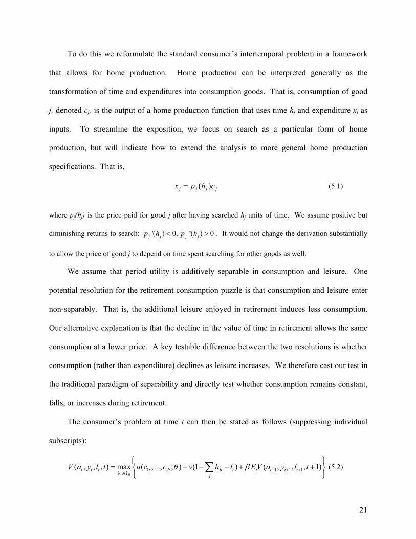
To do this we reformulate the standard consumer’s intertemporal problem in a framework

that allows for home production. Home production can be interpreted generally as the

transformation of time and expenditures into consumption goods. That is, consumption of good

j, denoted cj, is the output of a home production function that uses time hj and expenditure xj as

inputs. To streamline the exposition, we focus on search as a particular form of home

production, but will indicate how to extend the analysis to more general home production

specifications. That is,

( )j j j jx p h c= (5.1)

where pj(hj) is the price paid for good j after having searched hj units of time. We assume positive but

diminishing returns to search: '( ) 0, ''( ) 0j j j jp h p h< > . It would not change the derivation substantially

to allow the price of good j to depend on time spent searching for other goods as well.

We assume that period utility is additively separable in consumption and leisure. One

potential resolution for the retirement consumption puzzle is that consumption and leisure enter

non-separably. That is, the additional leisure enjoyed in retirement induces less consumption.

Our alternative explanation is that the decline in the value of time in retirement allows the same

consumption at a lower price. A key testable difference between the two resolutions is whether

consumption (rather than expenditure) declines as leisure increases. We therefore cast our test in

the traditional paradigm of separability and directly test whether consumption remains constant,

falls, or increases during retirement.

The consumer’s problem at time t can then be stated as follows (suppressing individual

subscripts):

1 1 1 1{ , }( , , , ) max ( ,..., ; ) (1 ) ( , , , 1)

jtt t t t Jt jt t t t t tc h j

V a y l t u c c v h l E V a y l tθ β + + +

= + − − + +

∑ (5.2)

22

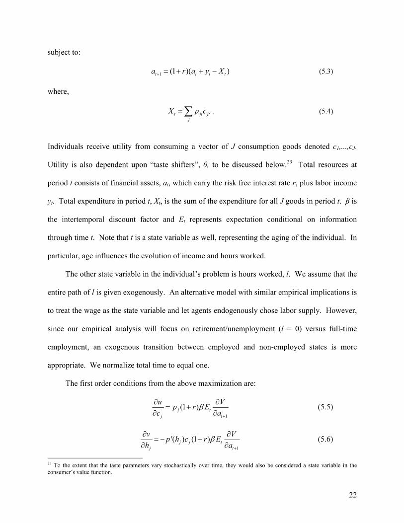
subject to:

1 (1 )( )t t t ta r a y X+ = + + − (5.3)

where,

t jt jtj

X p c=∑ . (5.4)

Individuals receive utility from consuming a vector of J consumption goods denoted c1,...,cJ.

Utility is also dependent upon “taste shifters”, θ, to be discussed below.23 Total resources at

period t consists of financial assets, at, which carry the risk free interest rate r, plus labor income

yt. Total expenditure in period t, Xt, is the sum of the expenditure for all J goods in period t. β is

the intertemporal discount factor and Et represents expectation conditional on information

through time t. Note that t is a state variable as well, representing the aging of the individual. In

particular, age influences the evolution of income and hours worked.

The other state variable in the individual’s problem is hours worked, l. We assume that the

entire path of l is given exogenously. An alternative model with similar empirical implications is

to treat the wage as the state variable and let agents endogenously chose labor supply. However,

since our empirical analysis will focus on retirement/unemployment (l = 0) versus full-time

employment, an exogenous transition between employed and non-employed states is more

appropriate. We normalize total time to equal one.

The first order conditions from the above maximization are:

1

(1 )j tj t

u Vp r Ec a

β+

∂ ∂= +

∂ ∂ (5.5)

1

'( ) (1 )j j tj t

v Vp h c r Eh a

β+

∂ ∂= − +

∂ ∂ (5.6)

23 To the extent that the taste parameters vary stochastically over time, they would also be considered a state variable in the consumer’s value function.

23

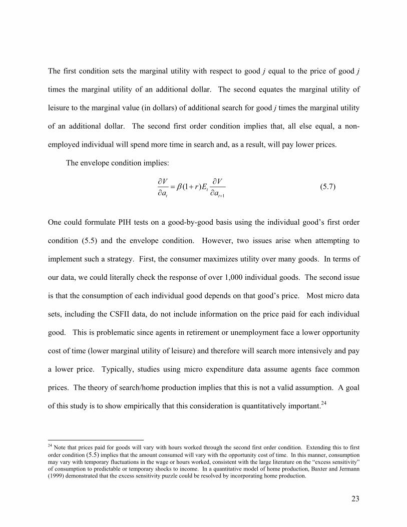
The first condition sets the marginal utility with respect to good j equal to the price of good j

times the marginal utility of an additional dollar. The second equates the marginal utility of

leisure to the marginal value (in dollars) of additional search for good j times the marginal utility

of an additional dollar. The second first order condition implies that, all else equal, a non-

employed individual will spend more time in search and, as a result, will pay lower prices.

The envelope condition implies:

1

(1 ) tt t

V Vr Ea a

β+

∂ ∂= +

∂ ∂ (5.7)

One could formulate PIH tests on a good-by-good basis using the individual good’s first order

condition (5.5) and the envelope condition. However, two issues arise when attempting to

implement such a strategy. First, the consumer maximizes utility over many goods. In terms of

our data, we could literally check the response of over 1,000 individual goods. The second issue

is that the consumption of each individual good depends on that good’s price. Most micro data

sets, including the CSFII data, do not include information on the price paid for each individual

good. This is problematic since agents in retirement or unemployment face a lower opportunity

cost of time (lower marginal utility of leisure) and therefore will search more intensively and pay

a lower price. Typically, studies using micro expenditure data assume agents face common

prices. The theory of search/home production implies that this is not a valid assumption. A goal

of this study is to show empirically that this consideration is quantitatively important.24

24 Note that prices paid for goods will vary with hours worked through the second first order condition. Extending this to first order condition (5.5) implies that the amount consumed will vary with the opportunity cost of time. In this manner, consumption may vary with temporary fluctuations in the wage or hours worked, consistent with the large literature on the “excess sensitivity” of consumption to predictable or temporary shocks to income. In a quantitative model of home production, Baxter and Jermann (1999) demonstrated that the excess sensitivity puzzle could be resolved by incorporating home production.

24

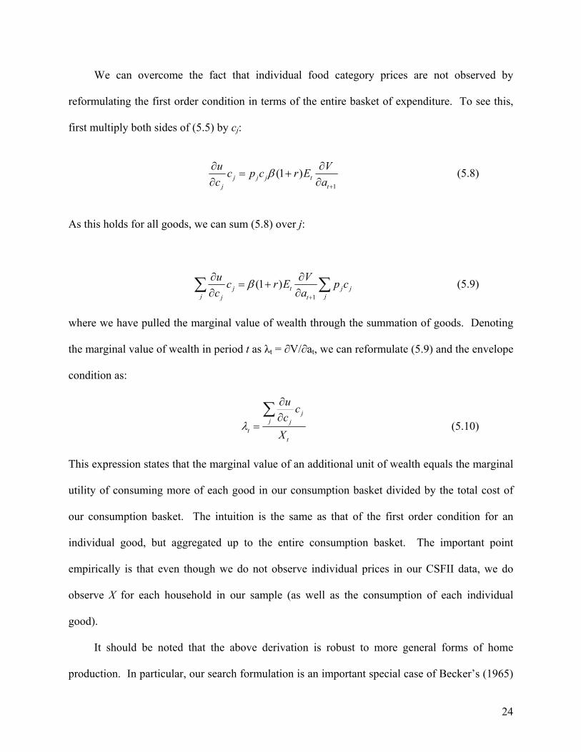
We can overcome the fact that individual food category prices are not observed by

reformulating the first order condition in terms of the entire basket of expenditure. To see this,

first multiply both sides of (5.5) by cj:

1

(1 )j j j tj t

u Vc p c r Ec a

β+

∂ ∂= +

∂ ∂ (5.8)

As this holds for all goods, we can sum (5.8) over j:

1

(1 )j t j jj jj t

u Vc r E p cc a

β+

∂ ∂= +

∂ ∂∑ ∑ (5.9)

where we have pulled the marginal value of wealth through the summation of goods. Denoting

the marginal value of wealth in period t as λt = ∂V/∂at, we can reformulate (5.9) and the envelope

condition as:

j

j jt

t

u cc

Xλ

∂∂

=∑

(5.10)

This expression states that the marginal value of an additional unit of wealth equals the marginal

utility of consuming more of each good in our consumption basket divided by the total cost of

our consumption basket. The intuition is the same as that of the first order condition for an

individual good, but aggregated up to the entire consumption basket. The important point

empirically is that even though we do not observe individual prices in our CSFII data, we do

observe X for each household in our sample (as well as the consumption of each individual

good).

It should be noted that the above derivation is robust to more general forms of home

production. In particular, our search formulation is an important special case of Becker’s (1965)

25

general model of home production: cj=f(xj,hj). Any such home production function which is

homogenous of arbitrary degree in expenditure has a similar empirical implication as that

derived above.25

We assume households have standard preferences over aggregate consumption (C) such

that:

1

( , )1Cu C e

σθθ

σ

−

=−

(5.11)

where

1( ,..... ).JC C c c= (5.12) We assume the aggregator function C is constant returns to scale.

Substituting (5.11) and (5.12) into (5.10), we can express the first order condition as:

1

ttt

t

C eX

σθλ

−

= (5.13)

where we have used the fact that C is CRS, implying (1 )jj

u c uc

σ∂= −

∂∑ (if σ=1,

jj

u c ec

θ∂=

∂∑ ) According to the permanent income hypothesis, if there is no news about

changes in lifetime resources associated with retirement, the discounted marginal utility of

wealth should be constant as a household transitions into retirement. In principle, this can be

tested using the log-linearized consumption Euler equation:26

25 The first order condition with respect to expenditure for good j is 1(1 )/ /

jx tj tf r Eu c V aβ += +∂ ∂ ∂ ∂ . Euler’s formula

states that xfx=sf (= scj) if f is homogenous of degree s in expenditure. Multiplying both sides of the FOC by xj and applying Euler’s formula yields an expression that differs from (5.9) only by the constant s. 26 Notice that (5.14) is nearly identical to the standard consumption Euler Equation for a model with no home production (see, for example, Zeldes (1989)). It only differs in that it is formed over a consumption aggregate C and it controls directly for changes in log total expenditures. The derivation of (5.14) is straightforward by taking the log of (5.13), using the envelope condition, and expressing consumption in terms of aggregate consumption.

26

, 1 0, 1 , 1 , 1 , 1 1ln( ) ln( )i i i i it t t t t x t t t t tC Retired X θω ω ω ω θ ε+ + + + +∆ = + ∆ + ∆ + ∆ + (5.14)

where i indexes the household head, Retired is a dummy variable equal to 1 if the household

head is retired, and θ is a vector of taste shifters. The interest rate is subsumed in the constant

term. Alternatively, we can test the proposition by working directly with the log level of the

marginal utility of wealth and equation (5.13):

( ) ( ) 0 1ln(1/ ) ( 1) ln lni i i i i i

t t t t t z t tC X Retired Zλ σ θ δ δ δ η= − + − = + + + (5.15) where Z is a vector of variables controlling for lifetime resources. We have expressed the left

hand side of (5.15) as the log inverse of the marginal utility of wealth for easy comparison with

(5.14).

If there is no news to the individual about their lifetime resources associated with

retirement, the permanent income hypothesis implies that consumption growth will not respond

to retirement aside from the impact of changes in price. This would imply that ω1 (from (5.14))

would be zero. Likewise, the marginal utility for individuals with similar lifetime resources will

be invariant to retirement status. This implies that δ1 from (5.15) will be zero. The alternative

hypothesis implicit in the retirement consumption puzzle (i.e., an increase in the marginal utility

of wealth at retirement) is that ω1 and δ1 are significantly negative.

In order to estimate (5.14) and (5.15), we must estimate the consumption index C.

Conditional on knowing aggregate consumption, C, we can compute the marginal utility of

wealth (from (5.13)). To do this, we assume that prime-aged, fully-employed household heads

satisfy the first order condition (5.13). The left hand side of (5.13) represents the marginal value

of wealth. This in turn is a function of lifetime resources, labor supply, and age. For estimation,

we assume that the cross section variation in lifetime resources is due to differences in labor

27

income (that is, agents start off with similar financial wealth and face the same rates of return

and time preference). We therefore approximate the log of the marginal utility of wealth as

being a linear function of log permanent income and a polynomial in age and employment hours

such that:

2 2

0 1 2 3ln( ) ln( ) ( ) ( ) ( ) ( )permt y t t t ty age age hours hoursλ ϕ ϕ ϕ ϕ ϕ ϕ≈ + + + + + (5.16)

Our estimation equation is then:

2 2

,0 1 1, ,

2 2

ln( ) .... ln( )

( ) ( )

perm i i i it J J t X t t

i i i i iage t t hours t t tage hours

y c c X

age age hours hours θβ α α β β θ

β β β β ε

= + + + + +

+ + + + + (5.17)

where we have linearized the term (1-σ)/φyln(C) over the individual components c1… cJ. This

approximation will be close given that each consumption good is essentially a zero/one variable.

Individuals, on any given day, only consume a handful of goods out of the hundreds of potential

food items. Most of the variation across individuals in the CSFII food intake data comes from

whether or not an individual eats a particular item, not how much of the item the individual

consumes. In this sense, our estimation essentially traces out a step function over the individual

goods. In Appendix 2, we discuss alternate specifications of the aggregate consumption

function.

The derivation is such that permanent income is our numeriere. This defines the units of

our consumption index ( 1 1 ... J Jc cα α+ + ) in terms of permanent income dollars – a one unit

increase in our consumption index is comparable to a one percent increase in permanent income.

We estimate equation (5.17) using a sample of households aged 25-55 who report working

full time. The vector of taste shifters, θ, include: a sex dummy, races dummies, household

composition dummies, the individual's height, and the full vector of household health controls

28

discussed in the Data Appendix. All regressions were run with and without year and region

dummies with no change in results. Restricting the estimation of (5.18) to a sample of household

heads aged 25-55 who report themselves employed full time leaves us with 2,966 individuals.

The permanent income for each employed household head is estimated as in section 4. For a list

of the food controls included in the regression see Appendix Table A4.

Before proceeding, we take a moment to interpret (5.18). In essence, we are projecting an

individual’s permanent income on their food intake and expenditure (along with demographic

and work intensity controls). In this sense, (5.18) provides the least-squares forecast of income

conditional on an individual’s diet. To explore how well food consumption predicts income, we

split the sample into two. We estimated (5.18) for individuals in the odd years of our survey.

The R-squared of this regression was 0.53. Food consumption items on their own explain 21%

of the variation in permanent income, while the incremental R-squared of the addition of the

food variables to the expenditure and demographic controls was 0.12. Using the regression

coefficients, we predicted permanent income out-of-sample for full-time employed individuals

aged 25-55 in the even years of the sample. The R-squared from this regression was 0.42

(omitting demographics and expenditure and using food alone produced an out-of-sample R-

squared of 0.09). This out-of-sample forecasting power indicates that diet is fairly informative

regarding permanent income.

From the estimation of (5.18), we obtained the parameters of the aggregation function and,

as a result, can form 1 1 Jˆ ˆ ˆln C c ... Jcα α≡ + + for each individual (including retired households).27

Figure 1 plots ˆln C for all household heads in the CSFII data between the ages of 57 and 71, by

three year age ranges. While expenditure falls dramatically for households in the peak 27 Note that we use the term l n C to refer to the estimated counterpart of the model’s (1 ) / ln( )y Cσ ϕ− , where concavity of the

value function implies φy <0 and conventional wisdom holds that σ>1.

29

retirement age, the consumption index remains essentially constant. This result is consistent

with the results from section 4. Households do not appear to change their diet in any discernable

way as they enter retirement. Figure 2 breaks down households by retirement status rather than

age and tells a similar story. For comparison, Appendix figure A1 plots aggregated consumption

and expenditure over the working-age life-cycle for full-time employed household heads.

Expenditure, despite being purged of household size effects,28 displays the familiar hump shape.

On the other hand, consumption itself increases relatively sharply between the ages of 25 and 37,

then remains relatively stable thereafter.29 We leave exploration of expenditure and consumption

early in the lifecycle for future research.

The second column of Table 5 reports the estimates of ω1 and δ1 from equations (5.14) and

(5.15). The first row of Table 5 reports the coefficient on retirement from specification (5.15),

where as usual we instrument retirement with age dummies. The second row replaces the

retirement dummy with a dummy variable indicating whether the household head is aged 63

years or older. The dependent variable is the fitted values of

x x1 1 Jˆ ˆ ˆln C ln X c ... ln XJcθ θβ β θ α α β β θ+ + = + + + + using the parameters estimated from

equation (5.17). Recall that our derivation implies that this measure is inversely proportional to

the log marginal utility of wealth. To account for the multiple steps in generating our dependent

variable, we bootstrap standard errors using 500 simulations. The sample used for the estimation

is the same as the sample used to estimate the regressions in Tables 1 and 4 and panel 2 of Tables

2 and 3. The regressions in Table 5, like those in earlier tables, are cross sectional in nature. In

essence, we estimate whether the marginal utility of wealth differs between non-retired and

28 Specifically, expenditure in Figure A1 is the residual from regressing log expenditure on dummy variables indicating household size. 29 Note that expenditure and consumption in figure A1 are in different units. Consumption is normalized by the elasticity of permanent income with respect to consumption. However, this normalization does not influence the shape of the consumption profile.

30

retired households after controlling for expected lifetime resources and demographics between

the two households. The results are striking: retired household heads (row 1) and heads older

than 63 (row 2) have the same marginal utility of wealth as their younger, non-retired

counterparts (and -0.01 and -0.003, respectively).30

The specifications underlying the first two rows of Table 5 relate the level of the marginal

utility of wealth to retirement status, controlling for determinants of lifetime resources. A

common alternative in the consumption literature tests for changes in marginal utility by

examining consumption Euler equations. Given the CSFII data, this task is complicated by the

absence of a panel. However, by averaging over similar individuals (i.e., creating synthetic

cohorts), we can follow representative individuals as they age through their life cycle.31 With

this constructed panel, we can test the Euler equation (5.14) directly. The advantage of this

procedure is that we relate changes in consumption directly to changes in retirement status. We

also eliminate some of the error associated with the individual level data. The downside of

course is we lose the informative individual variation as well. The results of estimating the Euler

equation are reported in third row of Table 5. Our estimate of ω1 from (5.14) is -0.002 (standard

error = 0.01), implying that the transition into retirement is not associated with an abrupt change

in the marginal utility of consumption.32

30 Lundberg et al. (2003), using data from the PSID, find that the decline in food expenditure at the time of retirement only occurs for married households. For single households in the PSID, expenditure remains constant through retirement. Using the Retirement History Survey, Haider and Stephens (2003) find that compared to married households, single households experience greater declines in expenditure at retirement. Using the CSFII data, we find that expenditure declines significantly for both single and married households, although the declines are larger for married households. The difference in results across the surveys is likely due to the small fraction of households that are of retirement age and are single. 31 More precisely, we define i to represent a group defined by sex, race, household size, and education. Let k represent employment status (full-time and retired), and t denote age. The sample is restricted to full-time or retired household heads

between the ages of 57 and 71. We construct ln,i k

tC by averaging ln C across individuals with a common triplet (i,k,t). Our

dependent variable is , , ' , , '

, 1 1ln ln lni k k i k i k

t t t tC C C+ +∆ = − . The retirement dummy takes a one if k=retired and k’=full-time and zero otherwise (we omit the case where k=full-time and k’=retired, i.e. the transition out of retirement). 32 The specification reported in Table 5 does not include controls for health and other demographics. We constructed group-level taste and demographic controls by averaging dummy variables within groups. That is, the percentage of a group which report

31

The results reported in Table 5 are robust to alternative samples and functional form

assumptions. In Appendix 2, we discuss a series of alternate specifications for (5.17). As seen

in Appendix Table A5, the alternate specifications yield nearly identical results to those reported

in Table 5.

A typical concern with finding that a variable has no effect is the power of the test: that is,

are we confident that our procedure would detect a significant effect if one indeed existed in the

population. The fact that our measure of the marginal utility of wealth based on consumption

and expenditure predicts permanent income out of sample is one argument against this concern.

Secondly, our measure includes expenditure directly, implying that if our food consumption

measures were meaningless, our index would simply track expenditure. Retirement clearly

predicts a drop in expenditure, suggesting our consumption measures are playing a significant

role in the analysis. 33 Finally, as we discuss in the next section, our consumption-based measure

of marginal utility responds to unemployment status. Given that there is news about changes in

permanent income associated with unemployment, we would expect the consumption index to

respond to job displacement. We shall see the test of the PIH introduced in this section is one

powerful enough to recognize unemployment as a shock to permanent income.

VI. Consumption Changes during Unemployment

As retirement is an essentially anticipated change in employment, it provides a clean test of

the PIH. The evidence presented in the previous two sections strongly indicates that the PIH,

augmented with search/home production, is consistent with the well-documented drop in

having high blood pressure etc. Including within-group differences (across age) as additional regressors does not change the result. The estimated coefficient on retirement was -0.005 with a standard error of 0.01. 33 Our measure of marginal utility includes log expenditure, which enters multiplied by the elasticity of permanent income with respect to expenditure. As intuition would suggest, this elasticity is positive and statistically significant. Of course, multiplying log expenditures by a constant does not alter the statistical significance of the effect of retirement on expenditure.

32

expenditure on food at retirement. In this section, we use the data and methodology developed

in the previous sections to analyze the change in the marginal utility of consumption when

workers become unemployed. To the extent that unemployment represents an unanticipated

shock to lifetime resources, the PIH does not predict that consumption will remain constant

across unemployment status. However, theory does suggest that unemployed agents should

spend more time in search/home production to reduce the price paid for a unit of consumption.

In this section, we explore the behavior of expenditure, time use and consumption across

employment status for the working age population. Our analysis focuses on the sample of

household heads between the ages of 25 and 55 that are either employed full-time or

unemployed. When analyzing the unemployed, we do not exclude the over sample of the poor

from the 1989-91 CSFII survey. The over-sample provides us with many more unemployed

individual. As a result, our CSFII sample consists of 3,874 household heads, 7% of which report

being unemployed. For time use, we restrict the NHAPS sample to working age individuals who

are either employed full-time or unemployed and report less than 6 hours of food production.

This leaves a sample of 3,364 individuals, 4.6% of which are unemployed.

As with retirement, we first document that unemployed households spend less on food than

their employed counterparts. Figure 3 indicates that monthly expenditure falls by a little more

than $100 in unemployment, or 20% of the average employed food bill of $530.34 To control for

other observables, we estimate

0 1 2ln( )it it it itx Unemployed Z vβ β β= + + + (6.1)

34 Using the PSID, Stephens (2001) finds that household food expenditure declines by roughly 10% following involuntary job loss of the household head. Using the British Family Expenditure survey, Banks, Blundell, and Tanner (1998) find unemployed households experience a 7.6% decline in food at home and domestic energy and a 52% decline in work-related expenses which include restaurant meals, transport, and adult clothing.

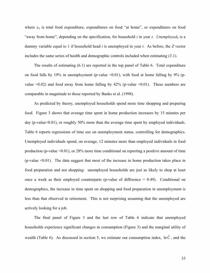
33

where xit is total food expenditure, expenditures on food “at home”, or expenditures on food

“away from home”, depending on the specification, for household i in year t. Unemployedit is a

dummy variable equal to 1 if household head i is unemployed in year t. As before, the Z vector

includes the same series of health and demographic controls included when estimating (3.1).

The results of estimating (6.1) are reported in the top panel of Table 6. Total expenditure

on food falls by 19% in unemployment (p-value <0.01), with food at home falling by 9% (p-

value =0.02) and food away from home falling by 42% (p-value <0.01). These numbers are

comparable in magnitude to those reported by Banks et al. (1998).

As predicted by theory, unemployed households spend more time shopping and preparing

food. Figure 3 shows that average time spent in home production increases by 15 minutes per

day (p-value<0.01), or roughly 50% more than the average time spent by employed individuals.

Table 6 reports regressions of time use on unemployment status, controlling for demographics.

Unemployed individuals spend, on average, 12 minutes more than employed individuals in food

production (p-value <0.01), or 28% more time conditional on reporting a positive amount of time

(p-value <0.01). The data suggest that most of the increase in home production takes place in

food preparation and not shopping: unemployed households are just as likely to shop at least

once a week as their employed counterparts (p-value of difference = 0.49). Conditional on

demographics, the increase in time spent on shopping and food preparation in unemployment is

less than that observed in retirement. This is not surprising assuming that the unemployed are

actively looking for a job.

The final panel of Figure 3 and the last row of Table 6 indicate that unemployed

households experience significant changes in consumption (Figure 3) and the marginal utility of

wealth (Table 6). As discussed in section 5, we estimate our consumption index, ˆln C , and the

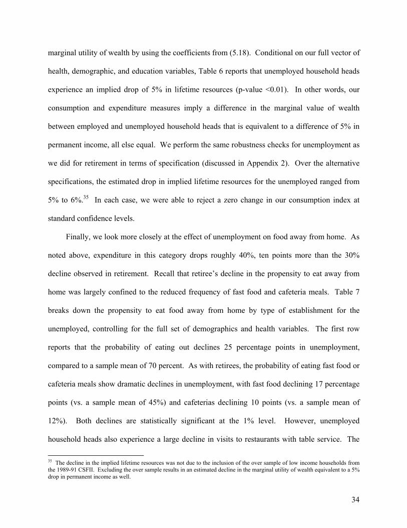
34

marginal utility of wealth by using the coefficients from (5.18). Conditional on our full vector of

health, demographic, and education variables, Table 6 reports that unemployed household heads

experience an implied drop of 5% in lifetime resources (p-value <0.01). In other words, our

consumption and expenditure measures imply a difference in the marginal value of wealth

between employed and unemployed household heads that is equivalent to a difference of 5% in

permanent income, all else equal. We perform the same robustness checks for unemployment as

we did for retirement in terms of specification (discussed in Appendix 2). Over the alternative

specifications, the estimated drop in implied lifetime resources for the unemployed ranged from

5% to 6%.35 In each case, we were able to reject a zero change in our consumption index at

standard confidence levels.

Finally, we look more closely at the effect of unemployment on food away from home. As

noted above, expenditure in this category drops roughly 40%, ten points more than the 30%

decline observed in retirement. Recall that retiree’s decline in the propensity to eat away from

home was largely confined to the reduced frequency of fast food and cafeteria meals. Table 7

breaks down the propensity to eat food away from home by type of establishment for the

unemployed, controlling for the full set of demographics and health variables. The first row

reports that the probability of eating out declines 25 percentage points in unemployment,

compared to a sample mean of 70 percent. As with retirees, the probability of eating fast food or

cafeteria meals show dramatic declines in unemployment, with fast food declining 17 percentage

points (vs. a sample mean of 45%) and cafeterias declining 10 points (vs. a sample mean of

12%). Both declines are statistically significant at the 1% level. However, unemployed

household heads also experience a large decline in visits to restaurants with table service. The

35 The decline in the implied lifetime resources was not due to the inclusion of the over sample of low income households from the 1989-91 CSFII. Excluding the over sample results in an estimated decline in the marginal utility of wealth equivalent to a 5% drop in permanent income as well.

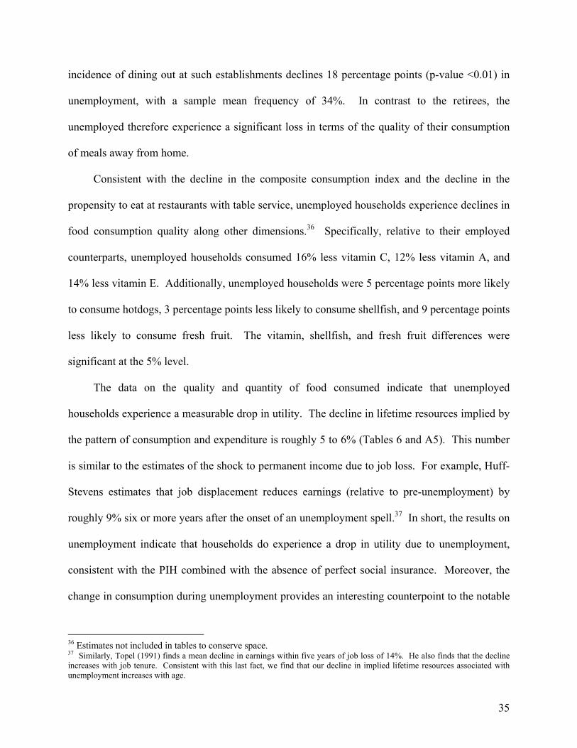
35

incidence of dining out at such establishments declines 18 percentage points (p-value <0.01) in

unemployment, with a sample mean frequency of 34%. In contrast to the retirees, the

unemployed therefore experience a significant loss in terms of the quality of their consumption

of meals away from home.

Consistent with the decline in the composite consumption index and the decline in the

propensity to eat at restaurants with table service, unemployed households experience declines in

food consumption quality along other dimensions.36 Specifically, relative to their employed

counterparts, unemployed households consumed 16% less vitamin C, 12% less vitamin A, and

14% less vitamin E. Additionally, unemployed households were 5 percentage points more likely

to consume hotdogs, 3 percentage points less likely to consume shellfish, and 9 percentage points

less likely to consume fresh fruit. The vitamin, shellfish, and fresh fruit differences were

significant at the 5% level.

The data on the quality and quantity of food consumed indicate that unemployed

households experience a measurable drop in utility. The decline in lifetime resources implied by

the pattern of consumption and expenditure is roughly 5 to 6% (Tables 6 and A5). This number

is similar to the estimates of the shock to permanent income due to job loss. For example, Huff-

Stevens estimates that job displacement reduces earnings (relative to pre-unemployment) by

roughly 9% six or more years after the onset of an unemployment spell.37 In short, the results on

unemployment indicate that households do experience a drop in utility due to unemployment,

consistent with the PIH combined with the absence of perfect social insurance. Moreover, the

change in consumption during unemployment provides an interesting counterpoint to the notable

36 Estimates not included in tables to conserve space. 37 Similarly, Topel (1991) finds a mean decline in earnings within five years of job loss of 14%. He also finds that the decline increases with job tenure. Consistent with this last fact, we find that our decline in implied lifetime resources associated with unemployment increases with age.

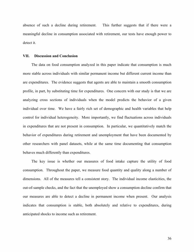
36

absence of such a decline during retirement. This further suggests that if there were a

meaningful decline in consumption associated with retirement, our tests have enough power to

detect it.

VII. Discussion and Conclusion

The data on food consumption analyzed in this paper indicate that consumption is much

more stable across individuals with similar permanent income but different current income than

are expenditures. The evidence suggests that agents are able to maintain a smooth consumption

profile, in part, by substituting time for expenditures. One concern with our study is that we are

analyzing cross sections of individuals when the model predicts the behavior of a given

individual over time. We have a fairly rich set of demographic and health variables that help

control for individual heterogeneity. More importantly, we find fluctuations across individuals

in expenditures that are not present in consumption. In particular, we quantitatively match the

behavior of expenditures during retirement and unemployment that have been documented by

other researchers with panel datasets, while at the same time documenting that consumption

behaves much differently than expenditures.

The key issue is whether our measures of food intake capture the utility of food

consumption. Throughout the paper, we measure food quantity and quality along a number of

dimensions. All of the measures tell a consistent story. The individual income elasticities, the

out-of-sample checks, and the fact that the unemployed show a consumption decline confirm that

our measures are able to detect a decline in permanent income when present. Our analysis

indicates that consumption is stable, both absolutely and relative to expenditures, during

anticipated shocks to income such as retirement.

37

While food consumption represents only a portion of the household's total consumption

bundle, the ability to shop for bargains and utilize other means of home production applies to

much broader classes of goods. Although we do not have direct data on consumption of other

goods, the analysis in this paper suggests that expenditure may be a misleading measure of

consumption more generally. This is supported by the fact that time shopping for non-food items

increase by 60% during retirement. However, what we can conclude directly from the evidence

in this paper is that any decline in total consumption due to temporary or anticipated fluctuations

in income occurs along dimensions other than food. This is perhaps expected given the fact that

food is a necessary good and amenable to home production. However, it provides an important

contrast to conclusions drawn from studies using food expenditures.

References

Angeletos, George-Marios, David Laibson, Jeremy Tobacman, Andrea Repetto and Stephen Weinberg (2001), “The Hyperbolic Consumption Model: Calibration, Simulation, and Empirical Evaluation, Journal of Economic Perspectives, August 2001, Vol 15 (3)

Attanasio, Orazio P. (1999), “Consumption”, in John Taylor and Michael Woodford, ed.

Handbook of Macroeconomics Vol 1B, Elsevier 1999. Banks, James, Richard Blundell, and Sarah Tanner (1998), “Is There a Retirement-

Savings Puzzle?", American Economic Review, Vol. 88 (4), pp. 769-788. Baxter, Marianne and Urban J. Jermann (1999), “Household Production and the Excess

Sensitivity of Consumption to Current Income”, American Economic Review, Vol. 89 (4), pp. 902-920.

Becker, Gary (1965), “A Theory of the Allocation of Time”, Economic Journal 75 (299),

pp. 493-508. Benhabib, Jess, Richard Rogerson, and Randall Wright (1991), “Homework in

Macroeconomics: Household Production and Aggregate Fluctuations”, Journal of Political Economy, Vol 99 (6), pp. 1166-1187.

Bernheim, B. Douglas, Jonathan Skinner, and Steven Weinberg (2001), “What Accounts

for the Variation in Retirement Wealth among U.S. Households?", American Economic Review, Vol. 91 (4), pp. 832-857.

Bhattacharya, Jayanta, Janet Currie, and Steven Haider (2001). "How Should We

Measure Hunger?" Working Paper. Bhattacharya, Jayanta, Janet Currie, and Steven Haider (2003). "Evaluating the Impact

of School Nutrition Programs," USDA Final Report. Blaylock, J.R. (1989), "An Economic Model of Grocery Shopping Frequency", Applied

Economics, 81(6), pp 843-52. Browning, Martin and Annamaria Lusardi (1996), “Household Savings: Micro Theories

and Micro Facts”, Journal of Economic Literature, Vol. 34 (4), pp. 1797-1855. Cronovich, Ron, Rennae Daneshvary, and R. Keith Schwer (1997), "The Determinants of

Coupon Usage," Applied Economics, 29, pp. 1631-41. Ghez, Gilbert and Gary Becker (1975). The Allocation of Time and Goods over the Life

Cycle, Columbia University Press, New York.

39

Greenwood, Jeremy and Zvi Hercovitz (1991), “The Allocation of Capital and Time over the Business Cycle,” Journal of Political Economy, Vol 99 (6), 1188-1214.

Greenwood, Jeremy, Richard Rogerson, and Randall Wright (1995), “Household

Production in Real Business Cycle Theory”, in Thomas Cooley, ed., Frontiers of Business Cycle Research, Princeton University Press, 1995.

Haider, Steven and Mel Stephens (2003), "Can Unexpected Retirement Expectations

Explain the Retirement Consumption Puzzle? Evidence from Subjective Retirement Expectations" Carnegie Mellon Working Paper.

Huff-Stevens, Ann (1997), “Persistent Effects of Job Displacement: The Importance of

Multiple Job Losses”, Journal of Labor Economics 15, 1, 165-88. Hurd, Michael and Susann Rohwedder (2003), “The Retirement-Consumption Puzzle:

Anticipated and Actual Declines in Spending at Retirement”, NBER Working Paper 9586,

Juster, F. Thomas and Frank Stafford (1985), ed. Time, Goods, and Well Being,

University of Michigan Press, 1985. Lundberg, Shelly, Richard Startz and Steven Stillman (2003). "The Retirement

Consumption Puzzle: A Marital Bargaining Approach", Journal of Public Economics, May, 1199-1218.

McGrattan, Ellen, Richard Rogerson, and Randall Wright (1997), “An Equilibrium

Model of the Business Cycle with Household Production and Fiscal Policy”, International Economic Review, Vol 38 (2), pp. 267-290.

Miniaci, Raffaele, Guglielmo Weber, and Chiara Monfardini (2002), “Is There a

Retirement Consumption Puzzle in Italy", working paper. Rios-Rull, Jose-Victor (1993), “Working in the Market, Working at Home, and the

Acquisition of Skills: A General-Equilibrium Approach”, American Economic Review, Vol 83 (4), pp. 893-907.

Rupert, Peter, Richard Rogerson, and Randall Wright (1995), “Estimating Substitution

Elasticities in Household Production Models”, Economic Theory, Vol 6, pp. 179-193.

Rupert, Peter, Richard Rogerson, and Randall Wright (2000), “Homework in Labor

Economics: Household Production and Intertemporal Substitution”, Journal of Monetary Economics, Vol 46, pp. 557-579.

Shapiro, Jesse (2003). "Is There a Daily Discount Rate? Evidence from the Food Stamps

Nutrition Cycle," Harvard University Working Paper.

40

Stephens, Mel (2001), “The Long-Run Consumption Effects of Earnings Shocks”,

Review of Economics and Statistics, Vol.83 (1), pp.28-36 Subramanian, Shankar and Angus Deaton (1996), "The Demand for Food and Calories",

Journal of Political Economy, 104 (1), pp. 133-62. Topel, Robert (1991), “Specific Capital, Mobility, and Wages: Wages Rise with Job

Seniority” Journal of Political Economy, Vol. 99 (1), pp. 145-176. Wilde, Parke E. and Christine Ranney (2000), "The Monthly Food Stamp Cycle: Shopping Frequency and Food Intake Decisions in an Endogenous Switching Regression Framework," Journal of Agricultural Economics, 82(1), pp. 200-213.

41

Appendix 1: Data Appendix For our primary analysis, we use data from the Continuing Survey of Food Intakes

by Individuals (CSFII) collected by the U.S. Department of Agriculture. Since the

1930's, the U.S. Department of Agriculture has conducted nationwide food surveys in

order to monitor the health and dietary habits of the U.S. population. The survey is cross

sectional in design and is administered at the household level. We make use of the two

most recent cross sectional surveys; the first interviewed households between 1989 and

1991 (CSFII_89) and the second interviewed households between 1994 and 1996

(CSFII_94). The two CSFII datasets collect information on the kinds and amounts of

foods eaten by Americans at home and away from home. Information on food eaten is

collected via an in-person interview on 2 (for the CSFII_94) or 3 (for the CSFII_89)

nonconsecutive days. Each day's information is collected using a 24-hour dietary recall.

Households were randomly chosen to participate in the survey. The entire sample

of the CSFII_94 and the main sample of the CSFII_89 were designed to be nationally

representative. The CSFII_89 included an over-sample of the poor. Unless we were

specifically looking at low-income households (including the unemployed), we restricted

our analysis to the CSFII_89's main sample. In conducting both surveys, interviewers

visited every sample address in person to inspect visually and to determine whether the

location represented a residential housing unit. In general, all selected households were

eligible to participate in the basic survey. However, households with nine or more

persons unrelated to the head of household were considered group quarters and were not

eligible. All related individuals in the selected household were eligible to participate in

the survey (roomers, borders, and employees were excluded). Persons who were living

42

away at school, traveling during the survey period, in military barracks, or in institutions

were also excluded.

The survey was conducted in stages. During the first stage, the interviewer (in

person) recorded household level data. This data included: age, educational levels,

employment status, race, and sex of each individual in the household; household size,

housing tenure, household income, food assistance program participation, and some other

food-related practices. During this interview, respondents were also asked to identify the

"male household head" (if present) and the "female household head" (if present). The

main meal planner for the household was also asked to report their usual expenditures on

food. Specifically, the following three questions were asked:

1. During the last three months, how much money has this household spent

per week (or per month) at grocery stores, including the stores' salad bars, soup bars,

delis. etc.? Include purchases made with food stamps.

2. During the last three months, how much has this household spent per week

(or per month) on food at specialty stores – such as bakeries, liquor stores, delicatessens,

meat markets, vegetable stands, health food stores, and other similar places – when the

food was brought into your home?

3. During the last three months, what has been this household's usual amount

of money spent per week (or per month) for food bought and eaten away from the home?

Include food and beverages that never entered your home, that is, eaten at restaurants,

fast food places, cafeterias at work or at school or purchased from vending machines, for

all household members?

43

During the CSFII_94, households were also explicitly asked to separate out fast

food expenditures from other food expenditures away from home. For our work, we

computed three food expenditure measures: total food expenditures, food expenditures at

home and food expenditures away from home. The total food expenditures summed

together all three of the above food expenditure questions; food at home summed only the

first two questions; and the third question represented food away from home. All food

expenditures were converted into monthly expenditures represented in 1996 dollars.

Aside from the expenditure questions, the CSFII respondents were asked to provide

detailed health questions. First, each individual was asked to self assess their own

health. This question is nearly identical in design to the self assessed health question

asked of Panel Study of Income Dynamic respondents. Specifically, the question reads

"In generally, would you say your health is excellent, very good, good, fair or poor?"

Aside from self assessing their own health, individuals were asked detailed

questions about their health history. In particular, the questionnaire includes “Has a

doctor every told you that you have diabetes?", and the same question repeated for high

blood pressure, heart disease, cancer, osteoporosis, high blood cholesterol, and stroke.

Lastly, individuals were asked to discuss past and current smoking behavior, report their

current height and weight, and indicate how much they exercise.

The main part of the CSFII data centers on the detailed food diaries. After

collecting the background information, the interviewer returned to the household within

the next few weeks to help the respondents complete a detailed food diary of the previous

day. The respondent was asked to report everything they ate or drank during the previous

44

24 hour period (starting at midnight of the prior day). Specifically, each individual

provided:

1. Detailed descriptions of all foods and beverages consumed (including brands); 2. Quantities eaten; 3. Time each eating occasion began; 4. Name of each eating occasion; 5. With whom the food was eaten; 6. Source of the food (from home food supply or obtained and eaten away from home). 7. Place from which food was obtained; and 8. Use of fat, salt, etc. in the food preparation (asked only of the main meal planner/preparer). The interviewers used standard household measuring cups and spoons and a ruler

during the interview to help each individual estimate quantities of foods and beverages

consumed. Under each food/drink category, there was a list of probing questions that the

interviewer was required to ask in order to collect enough detail for the food to be

properly coded. For example, probes included: "What was the brand name?", "Was your

(food item) regular, reduced calorie, high fiber, or something else?", or "Did you add any

spice or condiment to the food?". Additionally, the interviewer was directed to ask for

the ingredients to some food consumption (for example, what foods comprised

homemade soups, tacos, sandwiches, salads, casseroles, etc.). For each individual in the

survey, they completed multiple food diaries (three for the CSFII_89 and two for the

CSFII_94). The subsequent interviews were conducted similarly to the first. Households

were nominally compensated for their participation in the survey. Upon completion of

45

the survey, the Department of Agriculture converted the food diaries into more tangible

measures of nutrition (calories, protein (in grams), etc.). For the methodology and

software used for the conversion see www.barc.usda.gov/bhnrc/foodsurvey/home.htm.

For the work in this paper, we only used the multi-day average of nutritional measures for

each household. Lastly, it should be noted that it was required that at least 10% of the

food diaries covered every day of the week.

Given that the CSFII datasets are household surveys, we focus our analysis on the

expenditure and consumption behavior of the household head. As noted above,

expenditure is a household level variable while our consumption measures are at the

individual level. For most married couples, both the husband and the wife report

themselves as being a household head. In such instances, we follow the definition of

"household head" used in the Panel Study of Income Dynamics (PSID) and include only

the male household head in our analysis sample. Like the PSID, a female is only

considered a head of household if no male household head is present. This restriction 1)

ensures that we include only one member of each household in our empirical work and 2)

makes our work directly comparable to results found using the PSID.

Appendix Table A1 compares the pooled CSFII_89 and CSFII_94 data sets to the

1993 PSID. We focus on the PSID given that a large fraction of consumption research

uses that survey's food data. For comparison purposes, we restrict both samples to

include only household heads with ages between 22 and 65. The resulting sample sizes

were 7,350 for the pooled CSFII samples and 6,108 for the 1993 PSID sample. The

demographic composition of both samples closely mirrors each other. Appendix Table

46

A1 shows that the composition of households in the CSFII datasets is very similar to the

composition of households in the PSID.

47

Appendix 2: Empirical Robustness of Formal Test of PIH In this appendix we discuss the empirical robustness of the tests of the PIH

discussed in sections 5 and 6. Recall that our model implies agents equate the marginal

utility of wealth to the marginal utility of the consumption basket divided by total

expenditure (equation (5.13)). We used an approximation to this first order condition as a

basis for estimating the parameters of the consumption aggregator. We repeat our

estimation equation ((5.17)) below:

2 2

,0 1 1, ,

2 2

ln( ) .... ln( )

( ) ( )

perm i i i it J J t X t t

i i i i iage t t hours t t tage hours

y c c X

age age hours hours θβ α α β β θ

β β β β ε

= + + + + +

+ + + + +(5.17)

To check whether our results are sensitive to the particular approximation chosen, we

perform the analysis using several alternatives. That is, we estimate variants of (5.17),

and then use the estimated parameters to form alternative measures of the marginal utility

of wealth. As in sections 5 and 6, we then complete the analysis by regressing these

measures of marginal utility on dummy variables indicating retirement, age greater than

or equal to 63, and unemployment.

The results are reported in Table A5 with bootstrapped standard errors. The first

row replaces log expenditures with a quartic polynomial in expenditure in (5.17). The

second row restricts the sample for estimating (5.17) to fulltime workers who report

working between 40 and 50 hours per week (to eliminate any variation in employment

hours within the class of full-time employed). The third row includes all 188 3-digit food

categories (to allow a richer set of controls for consumption at the cost of overfitting

within sample). The fourth row replaces the quantity of each food item consumed with

48

zero-one dummy variables indicating a positive amount consumed. The fifth row

includes an age*hours interaction term. The final row restricts the analysis to white male

household heads to control for the fact that both tastes and incomes vary with race and

sex. The results are stable across the alternative specifications/samples, indicating that

the analysis is not sensitive to reasonable alternative functional forms or sample

selection.

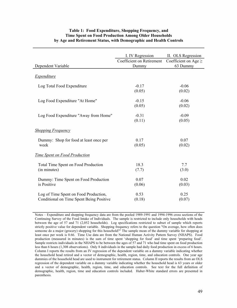
49

Table 1: Food Expenditure, Shopping Frequency, and Time Spent on Food Production Among Older Households

by Age and Retirement Status, with Demographic and Health Controls

I. IV Regression

II. OLS Regression

Dependent Variable

Coefficient on Retirement Dummy

Coefficient on Age ≥ 63 Dummy

Expenditure Log Total Food Expenditure -0.17 -0.06 (0.05) (0.02) Log Food Expenditure "At Home" -0.15 -0.06 (0.05) (0.02) Log Food Expenditure "Away from Home" -0.31 -0.09 (0.11) (0.05) Shopping Frequency Dummy: Shop for food at least once per week

0.17 (0.05)

0.07 (0.02)

Time Spent on Food Production Total Time Spent on Food Production (in minutes)

18.3 (7.7)

7.7 (3.0)

Dummy: Time Spent on Food Production is Positive

0.07 (0.06)

0.02 (0.03)

Log of Time Spent on Food Production, Conditional on Time Spent Being Positive

0.53 (0.18)

0.25 (0.07)

Notes – Expenditure and shopping frequency data are from the pooled 1989-1991 and 1994-1996 cross sections of the Continuing Survey of the Food Intake of Individuals. The sample is restricted to include only households with heads between the age of 57 and 71 (2,052 households). Log specifications restricted to subset of sample which reports strictly positive value for dependent variable. Shopping frequency refers to the question "On average, how often does someone do a major (grocery) shopping for this household?" The sample mean of the dummy variable for shopping at least once per week is 0.66. Time Use data are from the National Human Activity Pattern Survey (NHAPS). Food production (measured in minutes) is the sum of time spent ‘shopping for food’ and time spent ‘preparing food’. Sample restricts individuals in the NHAPS to be between the ages of 57 and 71 who had time spent on food production less than 6 hours (1,308 observations). Only 8 individuals in the sample had daily food production in excess of 6 hours. Column I reports the results from an IV regression of the dependent variable on a dummy variable indicating whether the household head retired and a vector of demographic, health, region, time, and education controls. One year age dummies of the household head are used to instrument for retirement status. Column II reports the results from an OLS regression of the dependent variable on a dummy variable indicating whether the household head is 63 years or older and a vector of demographic, health, region, time, and education controls. See text for the full definition of demographic, health, region, time and education controls included. Huber-White standard errors are presented in parenthesis.

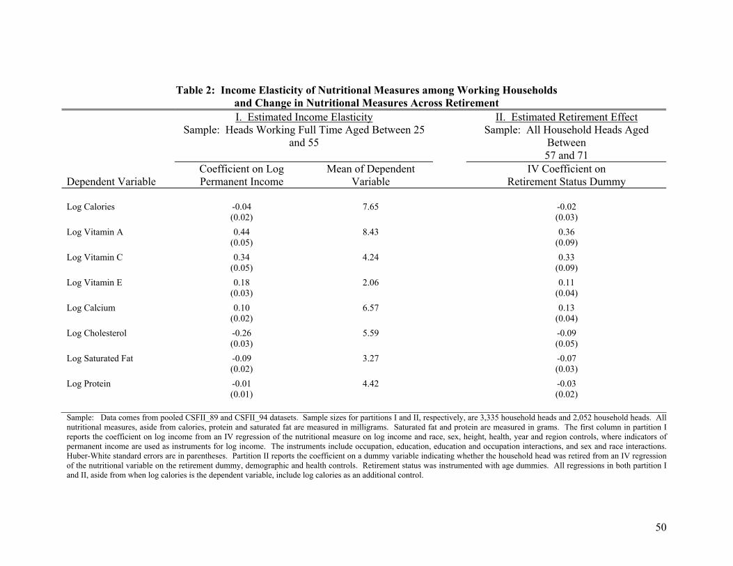
50

Table 2: Income Elasticity of Nutritional Measures among Working Households and Change in Nutritional Measures Across Retirement

I. Estimated Income Elasticity Sample: Heads Working Full Time Aged Between 25

and 55

II. Estimated Retirement Effect Sample: All Household Heads Aged

Between 57 and 71

Dependent Variable

Coefficient on Log Permanent Income

Mean of Dependent Variable

IV Coefficient on Retirement Status Dummy

Log Calories -0.04 7.65 -0.02 (0.02) (0.03) Log Vitamin A 0.44 8.43 0.36 (0.05) (0.09) Log Vitamin C 0.34 4.24 0.33 (0.05) (0.09) Log Vitamin E 0.18 2.06 0.11 (0.03) (0.04) Log Calcium 0.10 6.57 0.13 (0.02) (0.04) Log Cholesterol -0.26 5.59 -0.09 (0.03) (0.05) Log Saturated Fat -0.09 3.27 -0.07 (0.02) (0.03) Log Protein -0.01 4.42 -0.03 (0.01) (0.02) Sample: Data comes from pooled CSFII_89 and CSFII_94 datasets. Sample sizes for partitions I and II, respectively, are 3,335 household heads and 2,052 household heads. All nutritional measures, aside from calories, protein and saturated fat are measured in milligrams. Saturated fat and protein are measured in grams. The first column in partition I reports the coefficient on log income from an IV regression of the nutritional measure on log income and race, sex, height, health, year and region controls, where indicators of permanent income are used as instruments for log income. The instruments include occupation, education, education and occupation interactions, and sex and race interactions. Huber-White standard errors are in parentheses. Partition II reports the coefficient on a dummy variable indicating whether the household head was retired from an IV regression of the nutritional variable on the retirement dummy, demographic and health controls. Retirement status was instrumented with age dummies. All regressions in both partition I and II, aside from when log calories is the dependent variable, include log calories as an additional control.

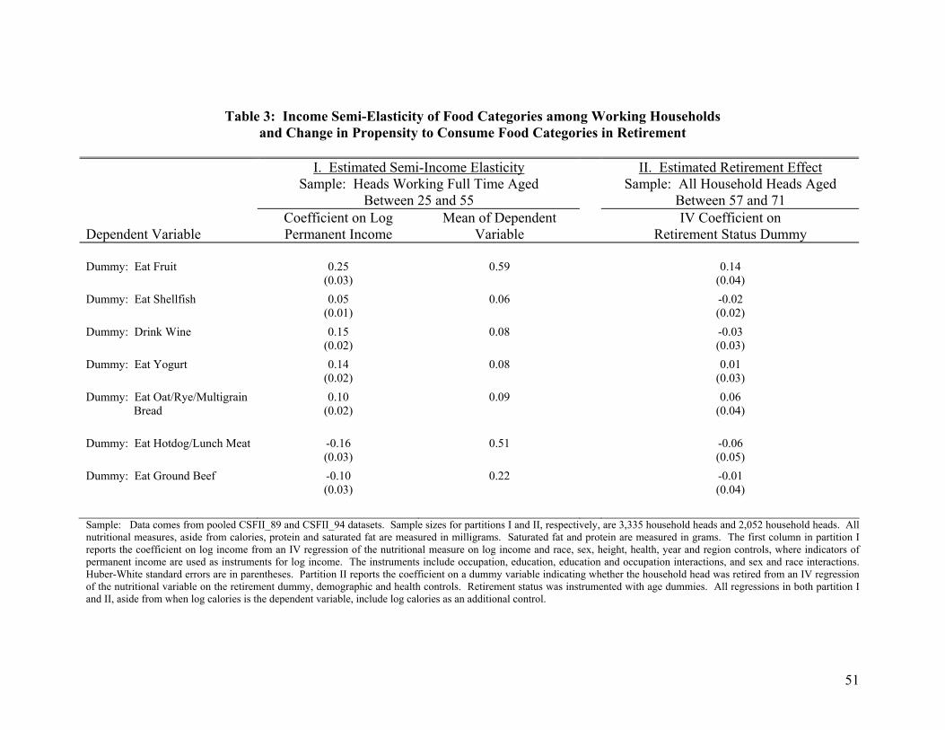
51

Table 3: Income Semi-Elasticity of Food Categories among Working Households and Change in Propensity to Consume Food Categories in Retirement

I. Estimated Semi-Income Elasticity

Sample: Heads Working Full Time Aged Between 25 and 55

II. Estimated Retirement Effect Sample: All Household Heads Aged

Between 57 and 71 Dependent Variable

Coefficient on Log Permanent Income

Mean of Dependent Variable

IV Coefficient on Retirement Status Dummy

Dummy: Eat Fruit 0.25 0.59 0.14 (0.03) (0.04) Dummy: Eat Shellfish 0.05 0.06 -0.02 (0.01) (0.02) Dummy: Drink Wine 0.15 0.08 -0.03 (0.02) (0.03) Dummy: Eat Yogurt 0.14 0.08 0.01 (0.02) (0.03) Dummy: Eat Oat/Rye/Multigrain Bread

0.10 (0.02)

0.09 0.06 (0.04)

Dummy: Eat Hotdog/Lunch Meat -0.16 0.51 -0.06 (0.03) (0.05) Dummy: Eat Ground Beef -0.10 0.22 -0.01 (0.03) (0.04)

Sample: Data comes from pooled CSFII_89 and CSFII_94 datasets. Sample sizes for partitions I and II, respectively, are 3,335 household heads and 2,052 household heads. All nutritional measures, aside from calories, protein and saturated fat are measured in milligrams. Saturated fat and protein are measured in grams. The first column in partition I reports the coefficient on log income from an IV regression of the nutritional measure on log income and race, sex, height, health, year and region controls, where indicators of permanent income are used as instruments for log income. The instruments include occupation, education, education and occupation interactions, and sex and race interactions. Huber-White standard errors are in parentheses. Partition II reports the coefficient on a dummy variable indicating whether the household head was retired from an IV regression of the nutritional variable on the retirement dummy, demographic and health controls. Retirement status was instrumented with age dummies. All regressions in both partition I and II, aside from when log calories is the dependent variable, include log calories as an additional control.

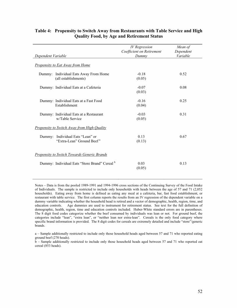
52

Table 4: Propensity to Switch Away from Restaurants with Table Service and High Quality Food, by Age and Retirement Status

Dependent Variable

IV Regression Coefficient on Retirement

Dummy

Mean of Dependent Variable

Propensity to Eat Away from Home Dummy: Individual Eats Away From Home (all establishments)

-0.18 (0.05)

0.52

Dummy: Individual Eats at a Cafeteria -0.07 0.08 (0.03) Dummy: Individual Eats at a Fast Food Establishment

-0.16 (0.04)

0.25

Dummy: Individual Eats at a Restaurant w/Table Service

-0.03 (0.05)

0.31

Propensity to Switch Away from High Quality Dummy: Individual Eats “Lean” or “Extra-Lean” Ground Beef a

0.13 (0.13)

0.67

Propensity to Switch Towards Generic Brands Dummy: Individual Eats “Store Brand” Cereal b 0.03 0.13 (0.05) Notes – Data is from the pooled 1989-1991 and 1994-1996 cross sections of the Continuing Survey of the Food Intake of Individuals. The sample is restricted to include only households with heads between the age of 57 and 71 (2,052 households). Eating away from home is defined as eating any meal at a cafeteria, bar, fast food establishment, or restaurant with table service. The first column reports the results from an IV regression of the dependent variable on a dummy variable indicating whether the household head is retired and a vector of demographic, health, region, time, and education controls. Age dummies are used to instrument for retirement status. See text for the full definition of demographic, health, region, time and education controls included. Huber-White standard errors are in parentheses. The 8 digit food codes categorize whether the beef consumed by individuals was lean or not. For ground beef, the categories include “lean”, “extra lean”, or “neither lean nor extra-lean”. Cereals is the only food category where specific brand information is provided. The 8 digit codes for cereals are extremely detailed and include “store”/generic brands.

a – Sample additionally restricted to include only those household heads aged between 57 and 71 who reported eating ground beef (270 heads). b – Sample additionally restricted to include only those household heads aged between 57 and 71 who reported eat cereal (853 heads).

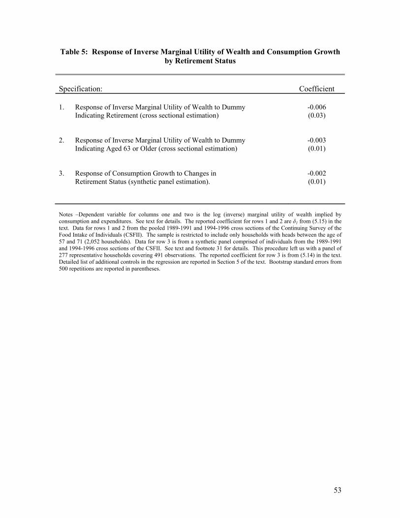
53

Table 5: Response of Inverse Marginal Utility of Wealth and Consumption Growth by Retirement Status

Specification:

Coefficient

1. Response of Inverse Marginal Utility of Wealth to Dummy Indicating Retirement (cross sectional estimation)

-0.006 (0.03)

2. Response of Inverse Marginal Utility of Wealth to Dummy Indicating Aged 63 or Older (cross sectional estimation)

-0.003 (0.01)

3. Response of Consumption Growth to Changes in Retirement Status (synthetic panel estimation).

-0.002 (0.01)

Notes –Dependent variable for columns one and two is the log (inverse) marginal utility of wealth implied by consumption and expenditures. See text for details. The reported coefficient for rows 1 and 2 are δ1 from (5.15) in the text. Data for rows 1 and 2 from the pooled 1989-1991 and 1994-1996 cross sections of the Continuing Survey of the Food Intake of Individuals (CSFII). The sample is restricted to include only households with heads between the age of 57 and 71 (2,052 households). Data for row 3 is from a synthetic panel comprised of individuals from the 1989-1991 and 1994-1996 cross sections of the CSFII. See text and footnote 31 for details. This procedure left us with a panel of 277 representative households covering 491 observations. The reported coefficient for row 3 is from (5.14) in the text. Detailed list of additional controls in the regression are reported in Section 5 of the text. Bootstrap standard errors from 500 repetitions are reported in parentheses.

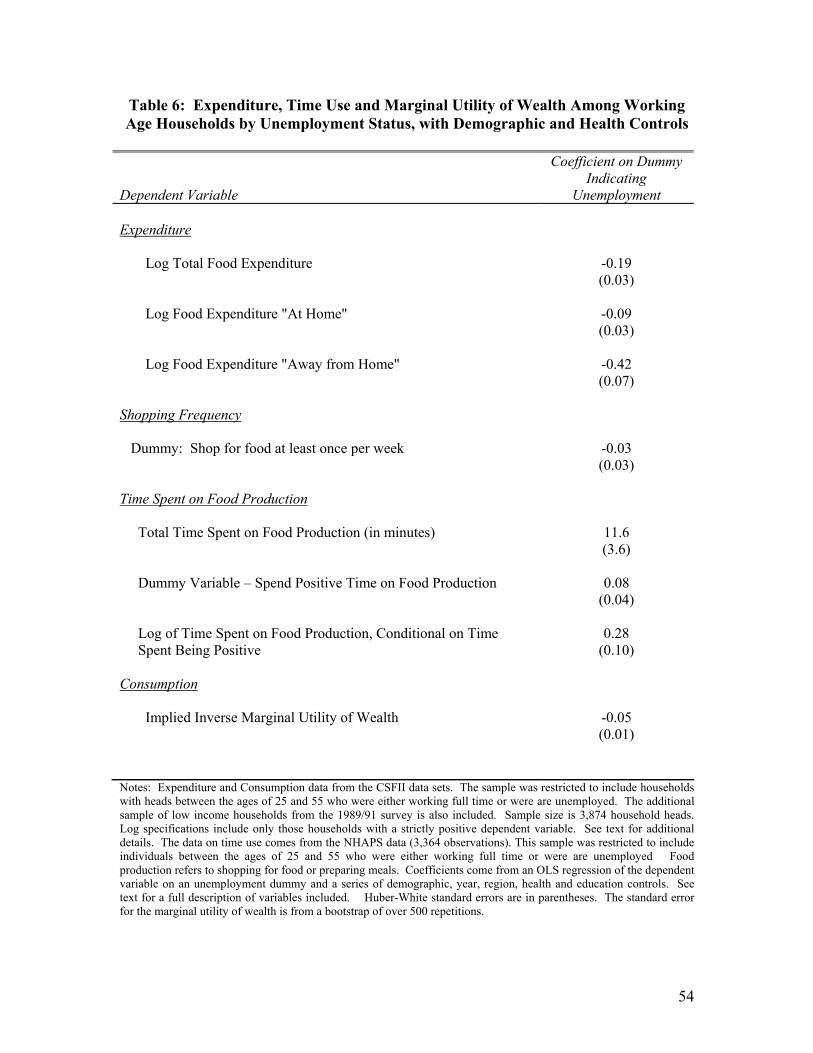
54

Table 6: Expenditure, Time Use and Marginal Utility of Wealth Among Working Age Households by Unemployment Status, with Demographic and Health Controls

Dependent Variable

Coefficient on Dummy Indicating

Unemployment Expenditure Log Total Food Expenditure -0.19 (0.03) Log Food Expenditure "At Home" -0.09 (0.03) Log Food Expenditure "Away from Home" -0.42 (0.07) Shopping Frequency Dummy: Shop for food at least once per week -0.03 (0.03) Time Spent on Food Production Total Time Spent on Food Production (in minutes) 11.6 (3.6) Dummy Variable – Spend Positive Time on Food Production 0.08 (0.04) Log of Time Spent on Food Production, Conditional on Time Spent Being Positive

0.28 (0.10)

Consumption Implied Inverse Marginal Utility of Wealth -0.05

(0.01) Notes: Expenditure and Consumption data from the CSFII data sets. The sample was restricted to include households with heads between the ages of 25 and 55 who were either working full time or were are unemployed. The additional sample of low income households from the 1989/91 survey is also included. Sample size is 3,874 household heads. Log specifications include only those households with a strictly positive dependent variable. See text for additional details. The data on time use comes from the NHAPS data (3,364 observations). This sample was restricted to include individuals between the ages of 25 and 55 who were either working full time or were are unemployed Food production refers to shopping for food or preparing meals. Coefficients come from an OLS regression of the dependent variable on an unemployment dummy and a series of demographic, year, region, health and education controls. See text for a full description of variables included. Huber-White standard errors are in parentheses. The standard error for the marginal utility of wealth is from a bootstrap of over 500 repetitions.

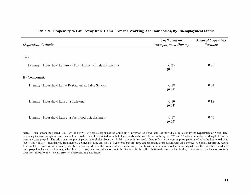
55

Table 7: Propensity to Eat "Away from Home" Among Working Age Households, By Unemployment Status

Dependent Variable

Coefficient on Unemployment Dummy

Mean of Dependent Variable

Total: Dummy: Household Eat Away From Home (all establishments) -0.25 0.70 (0.03) By Component: Dummy: Household Eat at Restaurant w/Table Service -0.18 0.34 (0.02) Dummy: Household Eats at a Cafeteria -0.10 0.12 (0.01) Dummy: Household Eats at a Fast Food Establishment -0.17 0.45 (0.03) Notes – Data is from the pooled 1989-1991 and 1994-1996 cross sections of the Continuing Survey of the Food Intake of Individuals, collected by the Department of Agriculture, excluding the over sample of low income households. Sample restricted to include households with heads between the ages of 25 and 55 who were either working full time or were are unemployed. The additional sample of poorer households from the 1989/91 survey is included. Data refers to the consumption patterns of only the household head (3,874 individuals). Eating away from home is defined as eating any meal at a cafeteria, bar, fast food establishment, or restaurant with table service. Column I reports the results from an OLS regression of a dummy variable indicating whether the household ate a meal away from home on a dummy variable indicating whether the household head was unemployed and a vector of demographic, health, region, time, and education controls. See text for the full definition of demographic, health, region, time and education controls included. Huber-White standard errors are presented in parentheses.

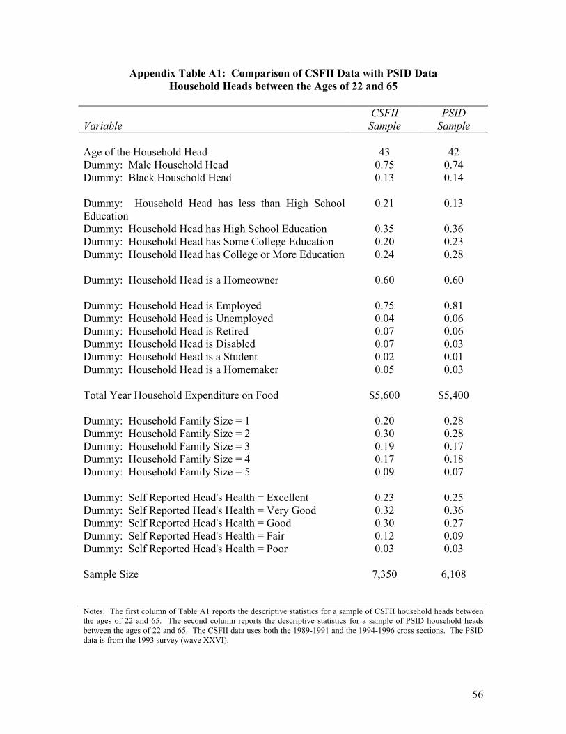
56

Appendix Table A1: Comparison of CSFII Data with PSID Data Household Heads between the Ages of 22 and 65

Variable

CSFII Sample

PSID Sample

Age of the Household Head 43 42 Dummy: Male Household Head 0.75 0.74 Dummy: Black Household Head 0.13 0.14 Dummy: Household Head has less than High School Education

0.21 0.13

Dummy: Household Head has High School Education 0.35 0.36 Dummy: Household Head has Some College Education 0.20 0.23 Dummy: Household Head has College or More Education 0.24 0.28 Dummy: Household Head is a Homeowner 0.60 0.60 Dummy: Household Head is Employed 0.75 0.81 Dummy: Household Head is Unemployed 0.04 0.06 Dummy: Household Head is Retired 0.07 0.06 Dummy: Household Head is Disabled 0.07 0.03 Dummy: Household Head is a Student 0.02 0.01 Dummy: Household Head is a Homemaker 0.05 0.03 Total Year Household Expenditure on Food $5,600 $5,400 Dummy: Household Family Size = 1 0.20 0.28 Dummy: Household Family Size = 2 0.30 0.28 Dummy: Household Family Size = 3 0.19 0.17 Dummy: Household Family Size = 4 0.17 0.18 Dummy: Household Family Size = 5 0.09 0.07 Dummy: Self Reported Head's Health = Excellent 0.23 0.25 Dummy: Self Reported Head's Health = Very Good 0.32 0.36 Dummy: Self Reported Head's Health = Good 0.30 0.27 Dummy: Self Reported Head's Health = Fair 0.12 0.09 Dummy: Self Reported Head's Health = Poor 0.03 0.03 Sample Size 7,350 6,108 Notes: The first column of Table A1 reports the descriptive statistics for a sample of CSFII household heads between the ages of 22 and 65. The second column reports the descriptive statistics for a sample of PSID household heads between the ages of 22 and 65. The CSFII data uses both the 1989-1991 and the 1994-1996 cross sections. The PSID data is from the 1993 survey (wave XXVI).

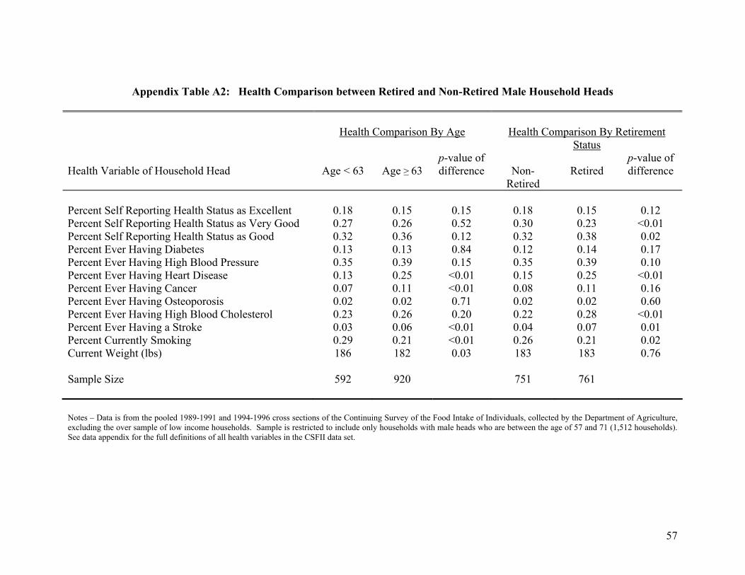
57

Appendix Table A2: Health Comparison between Retired and Non-Retired Male Household Heads

Health Comparison By Age

Health Comparison By Retirement

Status Health Variable of Household Head

Age < 63

Age ≥ 63

p-value of difference

Non-

Retired

Retired

p-value of difference

Percent Self Reporting Health Status as Excellent 0.18 0.15 0.15 0.18 0.15 0.12 Percent Self Reporting Health Status as Very Good 0.27 0.26 0.52 0.30 0.23 <0.01 Percent Self Reporting Health Status as Good 0.32 0.36 0.12 0.32 0.38 0.02 Percent Ever Having Diabetes 0.13 0.13 0.84 0.12 0.14 0.17 Percent Ever Having High Blood Pressure 0.35 0.39 0.15 0.35 0.39 0.10 Percent Ever Having Heart Disease 0.13 0.25 <0.01 0.15 0.25 <0.01 Percent Ever Having Cancer 0.07 0.11 <0.01 0.08 0.11 0.16 Percent Ever Having Osteoporosis 0.02 0.02 0.71 0.02 0.02 0.60 Percent Ever Having High Blood Cholesterol 0.23 0.26 0.20 0.22 0.28 <0.01 Percent Ever Having a Stroke 0.03 0.06 <0.01 0.04 0.07 0.01 Percent Currently Smoking 0.29 0.21 <0.01 0.26 0.21 0.02 Current Weight (lbs) 186 182 0.03 183 183 0.76 Sample Size 592 920 751 761 Notes – Data is from the pooled 1989-1991 and 1994-1996 cross sections of the Continuing Survey of the Food Intake of Individuals, collected by the Department of Agriculture, excluding the over sample of low income households. Sample is restricted to include only households with male heads who are between the age of 57 and 71 (1,512 households). See data appendix for the full definitions of all health variables in the CSFII data set.

58

Appendix Table A3: Sample of Detail of 8-Digit Food Categories in the CSFII 3-Digit Code Food Category 14010000 CHEESE, NFS 14010100 CHEESE,CHEDDAR/AMERICAN TYPE,NS NATURAL OR PROCESSED 14100100 CHEESE, NATURAL, NFS 14101010 CHEESE, BLUE OR ROQUEFORT 14102010 CHEESE, BRICK 14102110 CHEESE, BRICK, W/ SALAMI 14103010 CHEESE, CAMEMBERT 14103020 CHEESE, BRIE 14104010 CHEESE, NATURAL, CHEDDAR OR AMERICAN TYPE 14104020 CHEESE, CHEDDAR OR AMERICAN TYPE, DRY, GRATED 14104200 CHEESE, COLBY 14104250 CHEESE, COLBY JACK 14104400 CHEESE, FETA (INCLUDE GOAT CHEESE) 14104600 CHEESE, FONTINA 14104700 CHEESE, GOAT 14105010 CHEESE, GOUDA OR EDAM 14105200 CHEESE, GRUYERE 14106010 CHEESE, LIMBURGER 14106200 CHEESE, MONTEREY 14106500 CHEESE, MONTEREY, LOWFAT 14107010 CHEESE, MOZZARELLA, NFS (INCLUDE PIZZA CHEESE) 14107020 CHEESE, MOZZARELLA, WHOLE MILK 14107030 CHEESE, MOZZARELLA, PART SKIM (INCL ""LOWFAT"") 14107040 CHEESE, MOZZARELLA, LOW SODIUM 14107060 CHEESE, MOZZARELLA, NONFAT OR FAT FREE 14107200 CHEESE, MUENSTER 14107210 CHEESE, MUENSTER, LOW SODIUM 14107250 CHEESE, MUENSTER, LOWFAT 14108010 CHEESE, PARMESAN, DRY, GRATED (INCLUDE ROMANO) 14108020 CHEESE, PARMESAN, HARD (INCLUDE ROMANO) 14108050 CHEESE, PARMESAN, LOW SODIUM 14108060 PARMESAN CHEESE TOPPING, FAT FREE 14108200 CHEESE, PORT DU SALUT 14108400 CHEESE, PROVOLONE 14108410 CHEESE, PROVOLONE, REDUCED FAT & SODIUM 14108800 CHEESE, SEMI-SOFT, LOW SODIUM 14109010 CHEESE, SWISS 14109020 CHEESE, SWISS, LOW SODIUM 14109030 CHEESE, SWISS, LOWFAT 14110010 CHEESE, CHEDDAR OR COLBY, LOW SODIUM 14110020 CHEESE, CHEDDAR OR COLBY, LOW SODIUM, LOWFAT 14110030 CHEESE, CHEDDAR OR COLBY, LOWFAT 14131000 QUESO ANEJO (AGED MEXICAN CHEESE) 14131500 QUESO ASADERO (INCL OAXACAN-STYLE STRING CHEESE) 14132000 QUESO CHIHUAHUA (INCL MENNONITE CHEESE) 14133000 QUESO FRESCO (HISPANIC-STYLE FARMER CHEESE) 14200100 CHEESE, COTTAGE, NFS

59

Appendix Table A3: Sample of Detail of 8-Digit Food Categories in the CSFII

3-Digit Code Food Category 14201010 CHEESE, COTTAGE, CREAMED 14201200 COTTAGE CHEESE, FARMER'S 14201500 CHEESE, RICOTTA 14202010 CHEESE, COTTAGE, W/ FRUIT 14202020 CHEESE, COTTAGE, W/ VEGETABLES 14203010 CHEESE, COTTAGE, DRY CURD 14203020 CHEESE, COTTAGE, SALTED, DRY CURD 14203510 P.R. WHITE CHEESE (QUESO DEL PAIS, BLANCO) 14204010 CHEESE, COTTAGE, LOWFAT 14204020 CHEESE, COTTAGE, LOWFAT, W/ FRUIT 14204030 CHEESE, COTTAGE, LOWFAT, W/ VEGETABLES 14205010 CHEESE, COTTAGE, LOW SODIUM 14206010 CHEESE, COTTAGE, LOWFAT, LOW SODIUM 14207010 CHEESE, COTTAGE, LOWFAT, LACTOSE REDUCED 14210000 CHEESE, YOGURT, NFS 14220000 COTTAGE CHEESE, W/ FRUIT, BABY, NS AS TO STR OR JR 14301010 CHEESE, CREAM 14303010 CHEESE, CREAM, LOWFAT 14410100 CHEESE, PROCESSED, AMERICAN & SWISS BLENDS 14410200 CHEESE, PROCESSED, AMERICAN/CHEDDAR TYPE 14410210 CHEESE, PROCESSED, AMERICAN/CHEDDAR, LOW SODIUM 14410300 CHEESE, PROCESSED, AMERICAN/CHEDDAR TYPE, LOWFAT 14410310 CHEESE, PROCESSED, AMERICAN, LOWFAT, LOW SODIUM 14410330 CHEESE, PROC CHEESE PRODUCT, AMER/CHED, RED FAT 14410340 CHEESE,PROC CHEESE PROD,AMER/CHED,RED FAT & SODIU 14410350 CHEESE, PROCESSED, AMERICAN/CHEDDAR TYPE, NONFAT 14410380 CHEESE, PROCESSED CREAM CHEESE PRODUCT, NONFAT 14410400 CHEESE, PROCESSED, SWISS 14410410 CHEESE, PROCESSED, SWISS, LOW SODIUM 14410420 CHEESE, PROCESSED, SWISS, LOW FAT 14410440 CHEESE, PROCESSED, SWISS, LOW FAT, LOW SODIUM 14410450 CHEESE, PROCESSED CHEESE PRODUCT, SWISS, REDUCED FAT 14410500 CHEESE, PROCESSED, CHEESE FOOD 14410600 CHEESE, PROCESSED, W/VEGETABLES(INCL PEPPER CHEESE) 14410620 CHEESE, PROCESSED, W/ WINE 14410710 CHEESE, PROCESSED, MOZZARELLA, LOW SODIUM 14410830 CHEESE, PROCESSED, MUENSTER, LOWFAT, LOW SODIUM 14420000 CHEESE SPREAD, NFS 14420100 CHEESE SPREAD, AMERICAN OR CHEDDAR CHEESE BASE 14420140 CHEESE SPREAD, AMER/CHED BASE, LOW FAT, LOW SODIUM 14420160 CHEESE SPREAD, SWISS CHEESE BASE 14420200 CHEESE SPREAD, CREAM CHEESE OR NEUFCHATEL BASE 14420300 CHEESE SPREAD, PRESSURIZED CAN 14501010 IMITATION CREAM CHEESE 14502010 IMITATION CHEESE, AMERICAN OR CHEDDAR TYPE 14502040 IMITATION CHEESE, AMER/CHEDDAR TYPE, LOW CHOLESTERO 14503010 IMITATION CHEESE SPREAD (INCLUDE COUNT DOWN) 14504010 IMITATION MOZZARELLA CHEESE (INCL PIZZA MATE)

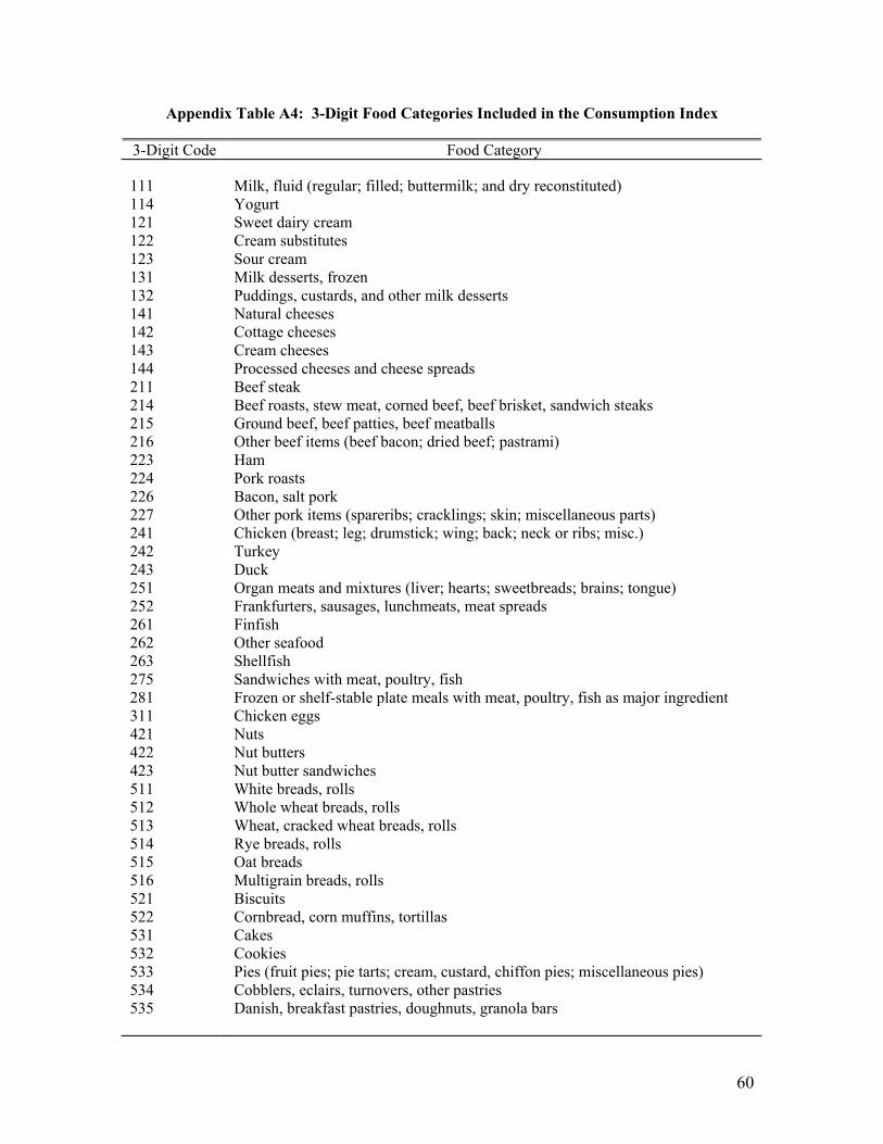
60

Appendix Table A4: 3-Digit Food Categories Included in the Consumption Index 3-Digit Code Food Category 111 Milk, fluid (regular; filled; buttermilk; and dry reconstituted) 114 Yogurt 121 Sweet dairy cream 122 Cream substitutes 123 Sour cream 131 Milk desserts, frozen 132 Puddings, custards, and other milk desserts 141 Natural cheeses 142 Cottage cheeses 143 Cream cheeses 144 Processed cheeses and cheese spreads 211 Beef steak 214 Beef roasts, stew meat, corned beef, beef brisket, sandwich steaks 215 Ground beef, beef patties, beef meatballs 216 Other beef items (beef bacon; dried beef; pastrami) 223 Ham 224 Pork roasts 226 Bacon, salt pork 227 Other pork items (spareribs; cracklings; skin; miscellaneous parts) 241 Chicken (breast; leg; drumstick; wing; back; neck or ribs; misc.) 242 Turkey 243 Duck 251 Organ meats and mixtures (liver; hearts; sweetbreads; brains; tongue) 252 Frankfurters, sausages, lunchmeats, meat spreads 261 Finfish 262 Other seafood 263 Shellfish 275 Sandwiches with meat, poultry, fish 281 Frozen or shelf-stable plate meals with meat, poultry, fish as major ingredient 311 Chicken eggs 421 Nuts 422 Nut butters 423 Nut butter sandwiches 511 White breads, rolls 512 Whole wheat breads, rolls 513 Wheat, cracked wheat breads, rolls 514 Rye breads, rolls 515 Oat breads 516 Multigrain breads, rolls 521 Biscuits 522 Cornbread, corn muffins, tortillas 531 Cakes 532 Cookies 533 Pies (fruit pies; pie tarts; cream, custard, chiffon pies; miscellaneous pies) 534 Cobblers, eclairs, turnovers, other pastries 535 Danish, breakfast pastries, doughnuts, granola bars

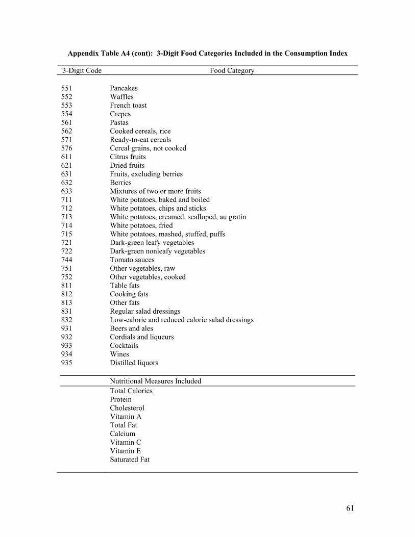
61

Appendix Table A4 (cont): 3-Digit Food Categories Included in the Consumption Index 3-Digit Code Food Category 551 Pancakes 552 Waffles 553 French toast 554 Crepes 561 Pastas 562 Cooked cereals, rice 571 Ready-to-eat cereals 576 Cereal grains, not cooked 611 Citrus fruits 621 Dried fruits 631 Fruits, excluding berries 632 Berries 633 Mixtures of two or more fruits 711 White potatoes, baked and boiled 712 White potatoes, chips and sticks 713 White potatoes, creamed, scalloped, au gratin 714 White potatoes, fried 715 White potatoes, mashed, stuffed, puffs 721 Dark-green leafy vegetables 722 Dark-green nonleafy vegetables 744 Tomato sauces 751 Other vegetables, raw 752 Other vegetables, cooked 811 Table fats 812 Cooking fats 813 Other fats 831 Regular salad dressings 832 Low-calorie and reduced calorie salad dressings 931 Beers and ales 932 Cordials and liqueurs 933 Cocktails 934 Wines 935 Distilled liquors Nutritional Measures Included Total Calories Protein Cholesterol Vitamin A Total Fat Calcium Vitamin C Vitamin E Saturated Fat

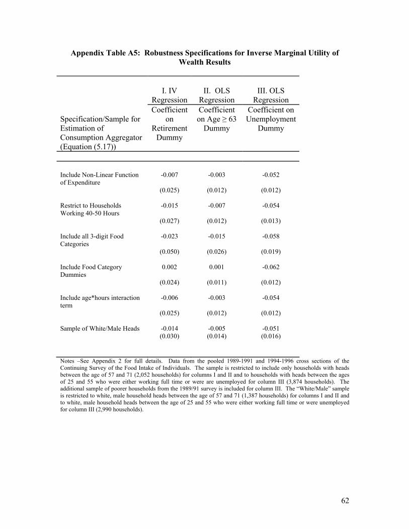
62

Appendix Table A5: Robustness Specifications for Inverse Marginal Utility of Wealth Results

I. IV Regression

II. OLS

Regression

III. OLS

Regression Specification/Sample for Estimation of Consumption Aggregator (Equation (5.17))

Coefficient on

Retirement Dummy

Coefficient on Age ≥ 63

Dummy

Coefficient on Unemployment

Dummy

Include Non-Linear Function of Expenditure

-0.007 -0.003 -0.052

(0.025) (0.012) (0.012) Restrict to Households Working 40-50 Hours

-0.015 -0.007 -0.054

(0.027) (0.012) (0.013) Include all 3-digit Food Categories

-0.023 -0.015 -0.058

(0.050) (0.026) (0.019) Include Food Category Dummies

0.002 0.001 -0.062

(0.024) (0.011) (0.012) Include age*hours interaction term

-0.006 -0.003 -0.054

(0.025) (0.012) (0.012) Sample of White/Male Heads -0.014 -0.005 -0.051 (0.030) (0.014) (0.016) Notes –See Appendix 2 for full details. Data from the pooled 1989-1991 and 1994-1996 cross sections of the Continuing Survey of the Food Intake of Individuals. The sample is restricted to include only households with heads between the age of 57 and 71 (2,052 households) for columns I and II and to households with heads between the ages of 25 and 55 who were either working full time or were are unemployed for column III (3,874 households). The additional sample of poorer households from the 1989/91 survey is included for column III. The “White/Male” sample is restricted to white, male household heads between the age of 57 and 71 (1,387 households) for columns I and II and to white, male household heads between the age of 25 and 55 who were either working full time or were unemployed for column III (2,990 households).

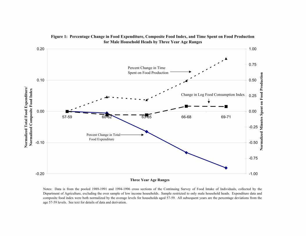
Figure 1: Percentage Change in Food Expenditure, Composite Food Index, and Time Spent on Food Production for Male Household Heads by Three Year Age Ranges

-0.20

-0.10

0.00

0.10

0.20

57-59 60-62 63-65 66-68 69-71

Three Year Age Ranges

Nor

mal

ized

Tot

al F

ood

Exp

endi

ture

/N

orm

aliz

ed C

ompo

site

Foo

d In

dex

-1.00

-0.75

-0.50

-0.25

0.00

0.25

0.50

0.75

1.00

Nor

mal

ized

Min

utes

Spe

nt o

n Fo

od P

rodu

ctio

n

Notes: Data is from the pooled 1989-1991 and 1994-1996 cross sections of the Continuing Survey of Food Intake of Individuals, collected by theDepartment of Agriculture, excluding the over sample of low income households. Sample restricted to only male household heads. Expenditure data andcomposite food index were both normalized by the average levels for households aged 57-59. All subsequent years are the percentage deviations from theage 57-59 levels. See text for details of data and derivation.

Percent Change in Total Food Expenditure

Change in Log Food Consumption Index

Percent Change in Time Spent on Food Production

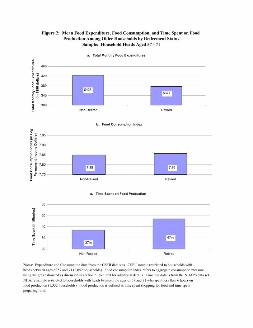
preparing food.

Sample: Household Heads Aged 57 - 71

NHAPS sample restricted to households with heads between the ages of 57 and 71 who spent less than 6 hours on food production (1,332 households). Food production is defined as time spent shopping for food and time spent

Figure 2: Mean Food Expenditure, Food Consumption, and Time Spent on Food Production Among Older Households by Retirement Status

Notes: Expenditure and Consumption data from the CSFII data sets. CSFII sample restricted to households withheads between ages of 57 and 71 (2,052 households). Food consumption index refers to aggregate consumption measureusing weights estimated as discussed in section 5. See text for additional details. Time use data is from the NHAPS data set.

c. Time Spent on Food Production

20

30

40

50

60

Non-Retired Retired

Tim

e Sp

ent (

in M

inut

es)

37m47m

a. Total Monthly Food Expenditures

300

340

380

420

460

Non-Retired RetiredTota

l Mon

thly

Foo

d Ex

pend

iture

s (in

199

6 do

llars

)

$423$377

b. Food Consumption Index

7.75

7.80

7.85

7.90

7.95

Non-Retired RetiredFood

Con

sum

ptio

n In

dex

(in L

og

Perm

anen

t Inc

ome

Dol

lars

)

7.85 7.86

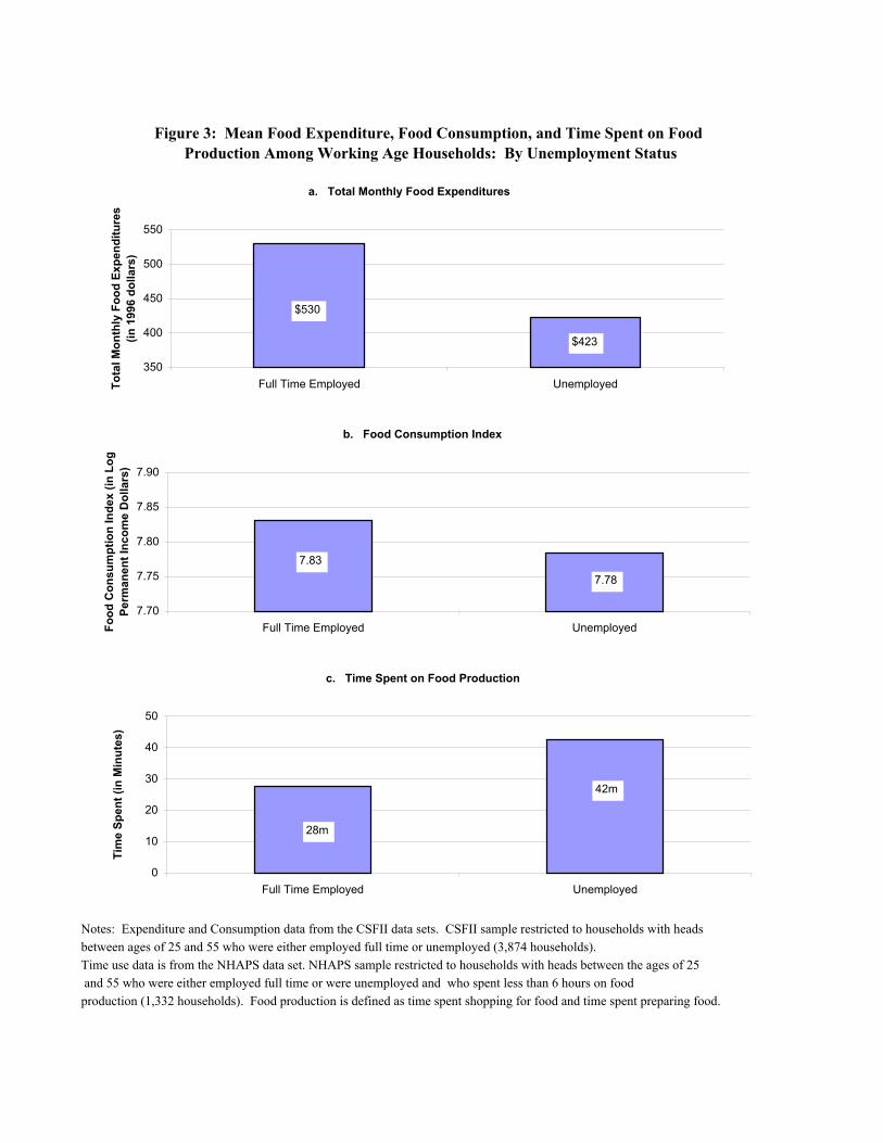
Figure 3: Mean Food Expenditure, Food Consumption, and Time Spent on Food Production Among Working Age Households: By Unemployment Status

Notes: Expenditure and Consumption data from the CSFII data sets. CSFII sample restricted to households with heads between ages of 25 and 55 who were either employed full time or unemployed (3,874 households).Time use data is from the NHAPS data set. NHAPS sample restricted to households with heads between the ages of 25 and 55 who were either employed full time or were unemployed and who spent less than 6 hours on food production (1,332 households). Food production is defined as time spent shopping for food and time spent preparing food.

c. Time Spent on Food Production

0

10

20

30

40

50

Full Time Employed Unemployed

Tim

e Sp

ent (

in M

inut

es)

28m

42m

a. Total Monthly Food Expenditures

350

400

450

500

550

Full Time Employed UnemployedTota

l Mon

thly

Foo

d Ex

pend

iture

s (in

199

6 do

llars

)

$530

$423

b. Food Consumption Index

7.70

7.75

7.80

7.85

7.90

Full Time Employed UnemployedFood

Con

sum

ptio

n In

dex

(in L

og

Perm

anen

t Inc

ome

Dol

lars

)

7.83

7.78

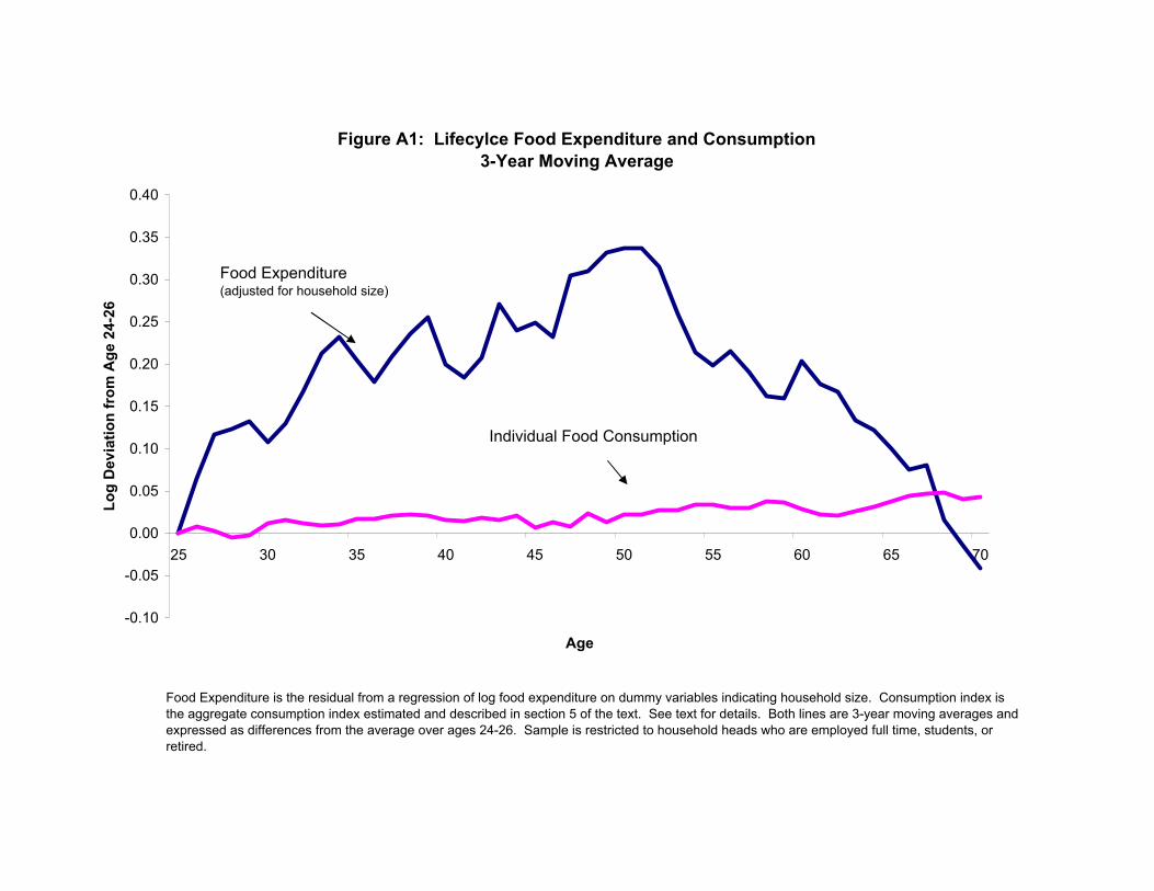
Figure A1: Lifecylce Food Expenditure and Consumption3-Year Moving Average

-0.10

-0.05

0.00

0.05

0.10

0.15

0.20

0.25

0.30

0.35

0.40

25 30 35 40 45 50 55 60 65 70

Age

Log

Dev

iatio

n fr

om A

ge 2

4-26

Food Expenditure is the residual from a regression of log food expenditure on dummy variables indicating household size. Consumption index is the aggregate consumption index estimated and described in section 5 of the text. See text for details. Both lines are 3-year moving averages and expressed as differences from the average over ages 24-26. Sample is restricted to household heads who are employed full time, students, or retired.

Food Expenditure(adjusted for household size)

Individual Food Consumption