GIFFEN BEHAVIOR AND SUBSISTENCE CONSUMPTION *

Robert T. Jensen The Watson Institute for International Studies

Brown University and

John F. Kennedy School of Government Harvard University

and NBER

Nolan H. Miller John F. Kennedy School of Government

Harvard University

January 2008

Forthcoming, American Economic Review Abstract: This paper provides the first real-world evidence of Giffen behavior, i.e., upward sloping demand. Subsidizing the prices of dietary staples for extremely poor households in two provinces of China, we find strong evidence of Giffen behavior for rice in Hunan, and weaker evidence for wheat in Gansu. The data provide new insight into the consumption behavior of the poor, who act as though maximizing utility subject to subsistence concerns, with both demand and calorie elasticities depending significantly, and non-linearly, on the severity of their poverty. Understanding this heterogeneity is important for the effective design of welfare programs for the poor. (JEL D01; I30; O12). KEYWORDS: Giffen Goods; Theory of the Consumer; Consumption; Poverty.

* We would like to thank Alberto Abadie, Chris Avery, Sebastian Bauhoff, Amitabh Chandra, Suzanne Cooper, Daniel Hojman, Brian Jacob, Elizabeth Lacey, Erzo Luttmer, Mai Nguyen, Albert Park, Rodrigo Wagner, Sangui Wang, and Richard Zeckhauser for valuable comments and discussions, and Frank Mou, Dulles Wang and Fan Zhang for research assistance. We gratefully acknowledge financial support from the National Institute of Aging, the William F. Milton Fund at Harvard Medical School, the Dean’s Research Fund at the John F. Kennedy School of Government, the Center for International Development at Harvard University, and the Hefner China Fund.

I. INTRODUCTION

The “Law of Demand,” which holds that as the price of a good increases, consumers’

demand for that good should decrease, is one of the bedrock principles of microeconomics.

However, economists have long recognized that the axioms of consumer theory do not guarantee

that demand curves must slope downward, and that the Law of Demand, while descriptively

valid in many situations, may not apply to very poor consumers facing subsistence concerns.

Alfred Marshall first publicized this idea in the 1895 edition of his Principles of Economics:

As Mr. Giffen has pointed out, a rise in the price of bread makes so large a drain on the resources of the poorer labouring families and raises so much the marginal utility of money to them, that they are forced to curtail their consumption of meat and the more expensive farinaceous foods: and, bread being still the cheapest food which they can get and will take, they consume more, and not less of it. (p. 208) Since Marshall’s time, a discussion of “Giffen” behavior has found its way into virtually

every basic economics course despite a lack of real-world evidence supporting Marshall’s

conjecture.1 Studies by Stigler (1947) and Koenker (1977) argue that neither demand for bread

nor demand for wheat was upward sloping in Britain during Marshall’s time. The standard

textbook example of a Giffen good (Samuelson, 1964), potatoes during the Irish famine of 1845-

1849, has also been discredited (Rosen, 1999). Not only are there no data to support the claim,

but at a more basic level it is unlikely that consumption of potatoes could have increased when

the price rose during the famine, at least in the aggregate, precisely because the price rise was

caused by a blight that destroyed much of the crop.2 While some laboratory studies have found

evidence of Giffen behavior, these experiments have been far from removed from reality.3

In this paper we present data from a field experiment exploring the response of poor

households in China to changes in the prices of staple food items that provide the first rigorous,

empirical evidence of real-world Giffen behavior. In fact, we find Giffen behavior with respect

to two goods, rice and wheat. Further, these goods, and the populations who exhibit Giffen

1 We use the term “Giffen behavior” rather than “Giffen good” to emphasize that the Giffen property is one that holds for particular consumers in a particular situation and therefore depends on, among other things, prices and wealth. Thus, it is not the good that is Giffen, but the consumers’ behavior. 2 Dwyer and Lindsay (1984) present a summary of the basic case against the potato version of the Giffen paradox. See also McDonough and Eisenhauer (1995). In both the bread and potato cases, it is possible that poor individuals exhibited Giffen behavior but the market overall did not. However, the data to test this hypothesis do not exist. 3 Battalio et al. (1991) find evidence of upward sloping demand among rats given limited “budgets” and the choice between root beer and a quinine solution, and DeGrandpre et al. (1993) find in a laboratory setting that human smokers given the choice between brands of cigarettes and a limited budget of “puffs” can exhibit Giffen behavior.

1

behavior, meet some basic but common conditions that suggest this behavior may be widespread

in the developing world. Thus, the absence of previously documented cases most likely results

from inadequate data or empirical strategies rather than from their non-existence.

Giffen behavior has long played an important, though controversial,4 role in economic

pedagogy, as well as in the history of economic thought. However, finding convincing evidence

of such behavior is important for economic theory more broadly. The fact that there has to date

been no convincing evidence of Giffen behavior stands as a minor embarrassment to economists

(Nachbar 1998), one that is reflected in the discussion of the Giffen phenomenon often being

presented as a paradox of economic theory rather than as a real (or even possible) mode of

behavior (e.g., Stigler, 1947). This lack of evidence has prompted a range of reactions among

economists. Some have interpreted it as support for the descriptive validity of the Law of

Demand:

Perhaps as persuasive a proof [of the ‘Law of Demand’] as is readily summarized is this: if an economist were to demonstrate its failure in a particular market at a particular time, he would be assured of immortality, professionally speaking, and rapid promotion while still alive. Since most economists would not dislike either reward, we may assume that the total absence of exceptions is not from lack of trying to find them. --George Stigler (1987, p.23). Others’ reactions to the lack of validation for the Giffen phenomenon have been more

extreme, interpreting it as an indictment of neoclassical consumer theory. Along these lines,

Boland (1977) points out that not only is the theory unable to rule out Giffen behavior, it is also

unable to explain why it is not observed. Put another way, if the neoclassical model is correct,

then under certain (albeit uncommon) conditions, Giffen behavior should exist. If it has not been

observed, it is either because the appropriate conditions have not been satisfied, the appropriate

data have not been available to measure it, or the theory is incomplete or flawed.5

4 The lack of verified examples has raised numerous concerns about the pedagogical role of the Giffen story: “Since the Giffen paradox is not useful for understanding the Irish Experience, is it asking too much for future writers of elementary texts to find another example? Fictions have no place in the teaching of economics,” Rosen (1999); “We shall have to find a new example of the positively sloping demand curve, or push our discussion of it deeper into footnotes,” Stigler (1947). 5 Others have argued that it is not our understanding of consumers that is flawed, but rather our understanding of markets. For example, Dougan (1982) argues that markets with upward sloping demand curves are inherently unstable, and thus unlikely to be observed, while Nachbar (1998) shows in a general equilibrium framework that observing the equilibrium price and quantity of a good move in the same direction in response to a supply shock implies that the commodity is normal, not inferior, and thus not Giffen at all. Thus economists looking for Giffen behavior at the level of the market are unlikely to find it.

2

Beyond documenting the existence of Giffen behavior, our field experiment also provides

an opportunity to study more broadly the consumption behavior of the “extreme poor,” a

population that worldwide includes more than one billion people living below the World Bank’s

extreme poverty line of one dollar per person per day. These households, like Marshall’s

“labouring families” and those in our sample, are often highly dependent on a single staple food

for the bulk of their nutritional needs. Consequently, fluctuations in the prices of these staple

foods can have large effects on real wealth and purchasing power. Anecdotally, such price

fluctuations, even fairly large ones, are increasingly common in developing countries.6 And

while there is a large literature examining household vulnerability and responses to income

shocks, there is comparably little evidence with respect to price shocks. Our analysis, by

focusing on the extremely poor and by introducing exogenous price changes for staple foods, is

useful for understanding this vulnerability.

In an earlier (unpublished) version of this paper (Jensen and Miller, 2002) using panel

data from the China Health and Nutrition Survey, we found suggestive evidence that poor

households in China exhibited Giffen behavior with respect to their primary dietary staple (rice

in the south, wheat and/or noodles in the north).7 However, because the study relied on possibly

endogenous variation in market prices, we were unable to identify a causal relationship between

price changes and consumption. To address this concern, for the present study we conducted a

field experiment in which for five months, randomly selected households were given vouchers

that subsidized their purchases of their primary dietary staple. Building on the insights of our

earlier analysis, we studied two provinces of China: Hunan in the south, where rice is the staple

good, and Gansu in the north, where wheat is the staple. Our analysis in these provinces focused

on households classified as the “urban poor,” a population that includes approximately 90

million individuals throughout China (Ravallion, 2007).

Using consumption surveys gathered before, during and after the subsidy was in place,

we find strong evidence that poor households in Hunan exhibit Giffen behavior with respect to

rice. That is, lowering the price of rice via the experimental subsidy caused households to reduce

6 For example, occasional reports from China note rice prices that double from year to year in some localities (“Surge in Consumer Prices Puts China on Guard,” China Daily, April 22, 2004). Friedman and Levinsohn (2002) note that the mean price of rice increased by almost 200 percent in Indonesia (where the typical household spends nearly 30 percent of its total household budget on rice) during the 1997/8 financial crisis.

3

their demand for rice, and removing the subsidy had the opposite effect. This finding is robust to

a wide range of empirical specifications. In Gansu, the evidence for Giffen behavior is somewhat

weaker, due to the partial failure of two of the basic conditions under which such behavior is

expected; namely that the staple good have limited substitution possibilities, and that households

are not so poor that they consume only staple foods. Focusing our analysis on those whom the

theory identifies as most likely to exhibit Giffen behavior, we find stronger evidence of its

existence.

We also provide important new insights into the consumption behavior of poor

households. In particular, we find the consumption response to an increase in the price of a staple

good follows a previously undocumented inverted-U pattern predicted by consumer theory in the

presence of subsistence concerns, with the very poorest and the least poor of the poor responding

by decreasing demand in response to an increase in the price of the staple in the standard way,

while the group in the middle increases demand (i.e., exhibits Giffen behavior). These results

have important implications for the design, targeting and evaluation of programs aimed at

improving nutrition among the poor.

The paper continues in Section II, where we present a discussion of the consumption

behavior of the poor that motivates Giffen behavior. Section III discusses the field experiment,

data, and estimation strategy. Section IV presents the results, and Section V concludes.

II. GIFFEN BEHAVIOR AND CONSUMPTION AMONG THE POOR

The conditions under which we would expect Giffen behavior can be demonstrated by

elaborating Marshall’s statement.8 Imagine an impoverished consumer near a subsistence level

of nutrition, whose diet consists of only two foods, a “basic” or staple good (in Marshall’s case,

bread) and a “fancy” good (meat). The basic good offers a high level of calories at low cost,

while the fancy good is preferred because of its taste but provides few calories per unit currency.

A poor consumer will therefore eat a lot of bread in order to get enough calories to meet his basic

needs and use whatever money he has left over to purchase meat. Now, if the price of bread

increases, he can no longer afford the original bundle of foods. And if he increases his

7 Ours is not the first study to suggest rice as a likely candidate for Giffen behavior. Dwyer and Lindsay (1984) propose (but do not test) this possibility for Singapore, and Chen (1994) finds suggestive evidence of positively sloped demand for rice in Taiwan.

4

consumption of meat, he will fall below his required caloric intake. So, he must instead increase

his consumption of bread (which is still the cheapest source of calories) and cut back on meat.

The Giffen phenomenon illustrates the potential significance of the wealth effects of price

changes for extremely poor households. Although the price increase makes the staple less

attractive in relative terms, the fact that it makes the consumer so much poorer (in real terms)

forces him to consume more bread. Translating this to the language of consumer theory, the

conditions under which Giffen behavior is likely to be observed therefore include that the good

in question be strongly inferior and that expenditure on that good comprise a large portion of the

consumer’s budget. As can be seen from the elasticity version of the Slutsky equation, εp = εph –

bεw, where εp is the observed price elasticity of demand, εph (≤ 0) is the Hicksian compensated

elasticity, εw is the wealth elasticity, and b is the budget share of the good, only then can the

wealth effect of a price increase be large enough to offset the pure substitution effect.

In light of these observations, we can state a set of conditions under which Giffen

behavior is most likely to be observed:9

C1: Households are poor enough that they face subsistence nutrition concerns.

C2: Households consume a very simple diet, including a basic (staple) and a fancy good.

C3: The basic good is the cheapest source of calories available, comprises a large part of the

diet/budget, and has no ready substitute.

When dealing with extreme poverty of the sort exhibited by the urban poor in China,

another requirement becomes important. While consumers who are too wealthy will not exhibit

Giffen behavior, those who are too poor also cannot exhibit Giffen behavior. To take an extreme

example, consider a consumer who is so poor that he only consumes bread. When the price of

bread increases, he has no choice but to consume less bread. Thus, it is critical to the Giffen story

that the consumer be consuming at least some of the fancy goods (e.g., meat) that are more

enjoyable but more expensive sources of calories so that he has something to substitute away

from when the price of the staple increases. In light of this, we add the following requirement to

the three stated above:

8 Much of the theory of Giffen behavior has previously appeared elsewhere. The interested reader should see the online appendix to this document for a discussion of the theory underlying this behavior. 9 Some of these conditions have been noted before by, for example, Gilley and Karels (1991).

5

C4: Households cannot be so impoverished that they consume only the staple good.

The theory thus predicts that only consumers that are poor, but not too poor, will exhibit

Giffen behavior. Panel A of figure 1 depicts the indifference curves for a typical consumer

choosing how much of the basic and fancy goods to consume. The basic or staple good is

relatively high in calories, while the fancy good offers more “taste,” i.e., the enjoyable but non-

nutritive aspects of food.10 The consumer’s indifference map can be divided into three regions.

The outer set of indifference curves correspond to the standard case, where the consumer’s

calorie intake is well above subsistence. Over this range the consumer trades off between

calories and taste (and thus between the basic and fancy goods) in an ordinary way. As the

consumer’s calorie consumption decreases, he crosses into a “subsistence zone.” Over this range,

caloric intake becomes much more important to the consumer. Consequently, the consumer’s

indifference curves take on the familiar “elbow” shape associated with Giffen behavior.11

Consumers in this range behave as if they maximize taste, subject to the constraint that they meet

their minimum caloric needs. As the consumer’s calorie consumption decreases even further, he

crosses from the subsistence zone to the calorie-deprived zone. In this region, the consumer’s

calorie intake is below subsistence levels. Hence, his primary concern is maximizing calories,

and the consumer’s indifference curves are, in effect, iso-calorie curves.

The consumer’s response to an increase in the price of the staple good will differ across

the three regions of his indifference map. When the consumer is relatively wealthy, he will

demand a bundle of goods in the standard zone. In this case, as illustrated in panel B of figure 1,

we expect the consumer to respond to an increase in the price of the staple good by consuming

less of it. Thus, demand is downward sloping. As wealth decreases, the consumer’s demand

moves into the subsistence zone, and the consumer focuses more on maintaining caloric intake as

his primary goal. It is over this region that Giffen behavior arises, as the consumer responds to an

increase in the price of the staple good by substituting toward the cheaper source of calories,

which is still the staple good. Over this range, the consumer still trades off calories against taste,

although caloric intake is given much greater importance. A consumer in the subsistence zone

10 The substitution across goods with varying nutritional and non-nutritional attributes also motivates the literature concerned with the income elasticity of demand for calories (see Strauss and Thomas 1995 and Deaton 1997). 11 See the online appendix for more discussion of the relationship between the shape of indifference curves needed to generate Giffen behavior and subsistence concerns.

6

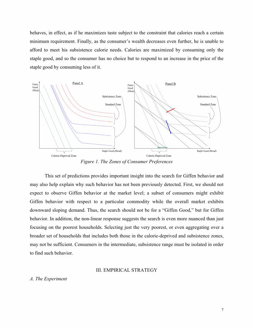
behaves, in effect, as if he maximizes taste subject to the constraint that calories reach a certain

minimum requirement. Finally, as the consumer’s wealth decreases even further, he is unable to

afford to meet his subsistence calorie needs. Calories are maximized by consuming only the

staple good, and so the consumer has no choice but to respond to an increase in the price of the

staple good by consuming less of it.

Standard Zone

Subsistence Zone

Calorie-Deprived Zone

Staple Good (Bread)

Fancy Good (Meat)

Standard Zone

Subsistence Zone

Calorie-Deprived Zone

Staple Good (Bread)

Fancy Good (Meat)

Panel A Panel B

Figure 1. The Zones of Consumer Preferences

This set of predictions provides important insight into the search for Giffen behavior and

may also help explain why such behavior has not been previously detected. First, we should not

expect to observe Giffen behavior at the market level; a subset of consumers might exhibit

Giffen behavior with respect to a particular commodity while the overall market exhibits

downward sloping demand. Thus, the search should not be for a “Giffen Good,” but for Giffen

behavior. In addition, the non-linear response suggests the search is even more nuanced than just

focusing on the poorest households. Selecting just the very poorest, or even aggregating over a

broader set of households that includes both those in the calorie-deprived and subsistence zones,

may not be sufficient. Consumers in the intermediate, subsistence range must be isolated in order

to find such behavior.

III. EMPIRICAL STRATEGY

A. The Experiment

7

A central problem in documenting Giffen behavior, and indeed in any analysis of

demand, is finding both sufficient and exogenous price variation. As a practical problem,

whether data are cross-sectional, time-series or panel, there is often not a great deal of variation

in prices for the kinds of goods likely to be candidates for Giffen behavior. This applies

especially to cross-sectional data, as arbitrage should eliminate spatial price differences,

especially for easily storable and non-perishable commodities such as grains. Further, the prices

for staple goods might even be fixed by the government for the poorest households, such as

under India’s Public Distribution System, and any remaining price variation may be due to

unobservable quality differences. A more serious concern is that even with sufficient price

variation, the source of that variation is often potentially endogenous, since price is the

equilibrium of a system of simultaneous equations. A positive correlation between price and

consumption could simply represent shocks to, or differences in, demand over space or time;

higher demand leads to higher prices, which could be misinterpreted as Giffen behavior.

Although instrumental variables could address this problem, finding instruments that shift supply

but do not directly affect demand is difficult.12

To overcome these challenges, we conducted a field experiment in which we provided

randomly selected poor households in two Chinese provinces with price subsidies for staple

foods. In Hunan, a southern province, rice is the staple good, and in Gansu, a northwestern

province, wheat is the staple good (consumed primarily as buns, a simple bread called mo or

noodles). These regional differences in preferences are primarily determined by geography,

climate and history, with wheat the dominant crop grown in Gansu and rice dominant in Hunan.

Accordingly, we subsidized rice (only) in Hunan and wheat flour (only) in Gansu.

Within each sample cluster (described below), households were randomly assigned to

either a control group or one of three treatment groups. Households in the treatment groups were

12 Most previous studies of Giffen behavior have failed to address this identification concern. A few cases have used instrumental variables, but with problematic instruments. For example, Bopp (1983) uses refinery utilization rates and the price of crude oil as instruments for the price of kerosene; however, both instruments likely also affect the price of substitute fuels, and are likely to be driven by other unobserved factors also affecting fuel demand, such as weather. Baruch and Kannai (2001) use the lagged prime interest rate as an instrument for the price of a low-grade Japanese alcohol (shochu), which is likely be a poor predictor of the price of shochu, or, to the extent that it does predict the price, will likely also affect the prices of substitutes (or income – and thus demand). Rainfall is commonly suggested as an instrument for price. However, rainfall will be an invalid instrument for the price of a given food item since it likely also affects the prices of other foods, as well as wages and income. One exception to the endogeneity concern in the search for Giffen behavior is McKenzie (2002), who uses the elimination of tortilla subsidies and price controls as a natural experiment to test for (and ultimately reject) such behavior in Mexico.

8

given printed vouchers entitling them to a price reduction of 0.10, 0.20 or 0.30 yuan (Rmb; 1

Rmb ≈$0.13) off the price of each jin (1 jin = 500g) of the staple good (the subsidy level stayed

fixed for each household over the course of the study). These subsidies represented substantial

price changes, since the average pre-intervention price of rice in Hunan was 1.2 yuan/jin, and the

average for wheat flour in Gansu was 1.04 yuan/jin. The vouchers were printed in quantities of 1,

5 and 10 jin, and the month’s supply of vouchers was distributed at the start of each month, with

each household receiving vouchers for 750g per person per day (about twice the average per

capita consumption). All vouchers remained valid until the end of the intervention. Households

were told in advance they would receive vouchers for five months and that any un-redeemed

vouchers would not be honored afterwards.

The vouchers could be redeemed at local grain shops. The merchants in these shops

agreed to honor the vouchers in exchange for reimbursement and a payment for their

participation. Households and merchants were told they were not permitted to exchange the

vouchers for anything but the staple good, that there would be periodic auditing and accounting

to make sure they were in compliance with the rules, and that any violations would result in them

being removed from the study without any additional compensation. Households and merchants

were explicitly told that selling the vouchers for cash or reselling rice or wheat bought with the

vouchers would result in dismissal from the program.

There are several points about the intervention worth noting. First, all foods in China are

sold in free markets, at market determined prices. A 1993 reform of the grain distribution system

largely put an end to price controls, state food stores, or free rations. Second, the number of

subsidized households in each sample site is trivial relative to the size of the population (all sites

were county seats, most with populations over one million), so the intervention could not have

affected market prices.13 Third, the experiment is predicated on the assumption that either

households are limited in their ability to borrow and save, or they have short planning horizons;

otherwise, the wealth effect of the five-month subsidy would be trivial, making Giffen behavior

unlikely. To the extent the wealth effect of the price change can be smoothed over the lifetime,

this will bias us against finding Giffen behavior. Fourth, limiting the quantity of vouchers to

750g/person/day might limit the potential demand response for the staple good (though the

13 Similarly, because the samples were drawn from lists of the poor spread throughout large cities, we believe it is unlikely the various study participants knew each other or the benefits others were receiving.

9

amount is still quite generous), but it should not induce Giffen behavior, as might be the case

(though still unlikely) if we limited the vouchers to a quantity smaller than what they would

prefer to consume.14 Finally, while staple foods such as rice can be found in varying qualities or

varieties with different prices, because the households in our sample are extremely poor, our data

show that they consume almost exclusively only the lowest-cost variety. Therefore, quality

substitution in response to the price subsidy is not a concern for our analysis. Two final concerns

with the experiment, namely whether there was cheating (in the form of cashing out or reselling)

despite our rules against doing so or whether the vouchers might create a “salience” or signaling

effect, are discussed with the results in section IV.E.

B. Data

The survey and intervention were conducted by employees of the provincial level

agencies of the Chinese National Bureau of Statistics. The sample consisted of 100-150

households in each of 11 county seats spread over Hunan and Gansu Provinces (Anren, Baoqing,

Longshan, Pingjiang, Shimen and Taojiang in Hunan, and Anding, Ganzhou, Kongdong,

Qingzhou and Yuzhong in Gansu), for a total of 1,300 households (650 in each province), with

3,661 individuals. Within each county, households were chosen at random from lists of the

“urban poor” maintained by the local offices of the Ministry of Civil Affairs.15 Households on

this list fall below a locally-defined poverty threshold (the Di Bao line), typically between 100

and 200 yuan per person per month or $0.41 − $0.82 per person per day, which is below even the

World Bank’s extreme poverty line of one dollar per person per day. It is estimated that about 90

million individuals throughout China live below the Di Bao threshold.

The questionnaire consisted of a standard income and expenditure survey, gathering

information on the demographic characteristics of household members as well as data on

employment, income, asset ownership and expenditures. A key component of the survey was a

24-hour food recall diary completed by each household member. Respondents were asked to

report everything they ate and drank the previous day, whether inside or outside the home, by

14 One concern is that by limiting the potential increase in consumption in response to the price decline, we might skew the average consumption change towards a decline (i.e., Giffen behavior). However, in practice almost no households even approached the voucher limit, most likely due to their extremely low incomes and a lack of access to credit, so this is unlikely to be a major concern.

10

specifically listing the components of all foods eaten.16 These foods were recorded in detail in

order to match with the 636 detailed food items listed in the 1991 Food Composition Tables

constructed by the Institute of Nutrition and Food Hygiene at the Chinese Academy of

Preventative Medicine. Though as we will see below, because households are very poor, most

diets are very simple and consist of a small number of basic (non -processed, -prepared or -

packaged) foods like rice, bean curd or stir-fried cabbage, so concerns about coding the specific

quantities of the various ingredients in a complex dish or meal are not significant.17

Data were gathered in three waves, conducted in April, September and December of

2006. After completing the first survey, treatment households were told they would receive the

subsidies for five months, from June through October. Thus, the initial interviews occurred

before treatment households knew of or received the subsidies, the second occurred after the

subsidy had been in place for slightly more than 3 months, and the final interviews were

conducted 1 to 2 months after the subsidy had ended, by which time treatment households would

likely have exhausted any stocks of rice or wheat flour they may have purchased with the

subsidy, and will therefore again be purchasing at the full market price. Sample attrition was

extremely low, since the three rounds occurred in a relatively short span. Only 11 of 1,300

households (<1%) in the first round did not appear in the second round. All households in the

second round were interviewed in the third round. Means and standard deviations for key

variables are presented in table 1.18

Table 2 shows the basic consumption patterns for households in the two provinces. The

dominance of, and difference in, staple goods in the two regions is evident. In Hunan, the

average per capita consumption of rice per day is 330g, comprising 64 percent of daily caloric

intake. The consumption of wheat is much lower, with only 42g of daily consumption per person

15 We chose urban areas because in smaller towns or rural areas many of the poorest households grew rather than purchased their staple food, and lower population density meant fewer households living in extreme poverty, which would have both required a greater number of sample clusters and prevented varying the treatment within clusters. 16 While it may seem difficult to recall or estimate how many grams of, say, rice was eaten with a meal, for the extreme poor who are on a very limited budget, food is often apportioned and accounted for much more carefully. Further, diets for these extremely poor households often vary little or not at all from day-to-day, except on special occasions, so recalling the quantity of specific food items is not as difficult. 17 Similarly, because households were so poor, almost all food (98 percent) was at-home consumption, so respondents were aware of the exact ingredients and quantities used. 18 While there are some differences in variables across control and treatment groups, these arise largely due to random variation given the relatively small sample size. Randomization was done blindly by the authors, rather than the field teams, so any differences should not be systematic. Further, any differences in variables across households based on treatment assignment will be eliminated because our analysis uses household fixed effects.

11

on average, comprising just 8 percent of total caloric intake. By contrast, Gansu features almost

the exact reverse pattern; wheat-based foods are the dominant staple, with 344g of consumption

per person per day, comprising 69 percent of total calories, whereas rice consumption is only

35g. In both provinces, the relevant staple good is a dominant source of calories for most

households, with 80 percent of households in Hunan relying on rice for at least half their calories

and 75 percent of households in Gansu similarly relying on wheat.19

The reliance on these basic foods for nutrition is underscored even more by the fact that

the average total calorie share from all cereals or grains is 72 percent in Hunan and 77 percent in

Gansu. Further, in both provinces, on average 13 percent of calories come from edible oils

(mostly vegetable oil), which is primarily used in cooking, and is generally not a substitute for

other forms of consumption or nutrition. Thus, the consumption of all other foods combined on

average contributes only 10 percent of calories in Gansu, and 15 percent in Hunan. In Hunan, the

greatest remaining share comes from meat, with 42 grams of consumption per person per day on

average, comprising 7 percent of average caloric intake. By contrast, in Gansu meat consumption

is much lower, averaging only 13 grams per person per day and contributing less than 1 percent

of total caloric intake. Consumption of pulses is in fact greater than consumption of meat in

Gansu. This is likely due to the lower income levels in this province; pulses are often referred to

as “poor man’s meat” because they are a cheaper source of protein (when combined with other

foods typically eaten as staples). Therefore, while the consumption patterns in Hunan match up

well with the basic conditions under which we predict Giffen behavior, in Gansu the patterns do

not fit quite as well due to relatively low consumption of meat (the fancy good in our set up).

C. Estimation Strategy

Given the random assignment of the price change and the panel nature of our survey, our

basic strategy is to simply compare the household-level changes in dietary intake20 of the staple

good for treatment and control groups. Since assignment to treatment and control groups was

19 These goods also fit the basic Giffen conditions in that they are the cheapest source of calories in each province: rice in Hunan yields 1399 calories/yuan, while wheat in Gansu yields 1655 calories/yuan. By contrast, the calories per yuan for other common foods are: wheat (1221), millet (537), pork (331), bean curd (239), and cabbage (141) in in Hunan, and millet (1105), rice (980), pork (340), bean curd (224), and cabbage (173) for Gansu. 20 While we also gathered data on food purchases and expenditures, actual daily intake is likely to be a better measure of consumption or demand. This is due to the fact that food is storable, purchases are lumpy or infrequent, and households’ recall of what they ate the day before the survey is likely to be significantly more accurate than recall of purchases over the past month.

12

randomized within sample counties, we add county*time fixed effects, so that we are in effect

comparing the changes for households with different subsidy levels within the same community.

This strategy controls for any county-level factors that change over time, such as the prices of

foods, labor market conditions or the value of government transfer programs.

We regress the percent change in intake of the staple good for household i in period t on

the change in the subsidy (in percent). The percent change formulation normalizes for factors

such as household size, composition, and activity level and allows us to interpret the coefficients

as elasticities. For each household, we observe two changes: the change between periods 2 and 1

(t = 2), capturing the effect of imposing the subsidy, and the change between periods 3 and 2 (t =

3), capturing the effect of removing the subsidy. Thus we estimate:

, , , ,% % % *i t i t i t i t i tstaple p Z County Time ,α β γ δΔ = + Δ + Δ + + Δ∑ ∑ ε (1)

where %Δstaplei,t is the percent change in household i’s consumption of the staple good, %Δpi,t

is the percent change in the price of the staple due to the subsidy (negative for t = 2 and positive

for t = 3), %ΔZ is a vector of percent changes in other control variables including income (split

into earned and unearned (government payments, pensions, remittances, rent and interest from

assets) sources) and household size, and County*Time denotes a set of county*time dummy

variables. We compute all changes as arc-percent-changes (i.e., 100*(xt – xt-1) / ((xt+xt-1) /2)).21

The percent change in the subsidy is computed as 100 times the change in the subsidy divided by

the average (net of subsidy) price of the staple good in the two corresponding rounds. The results

are robust to a wide range of alternative specifications, some of which we discuss in section

IV.B.

D. Refining the Test for Giffen Behavior

The discussion in section II highlighted a nuanced prediction of the standard consumer

model in light of subsistence concerns. The poorest of the poor should have a negative price

elasticity, the poor-but-not-too-poor may have a positive price elasticity, i.e., exhibit Giffen

behavior, and the relatively wealthy should once again have a negative price elasticity. Although

our primary concern in this paper is documenting the presence of Giffen behavior, we are also

interested in testing this broader prediction of the theory.

13

Unfortunately, classifying households or individuals directly by consumption zone is not

possible. Not only is there no consensus on what constitutes a subsistence level of calories, but

any such threshold would certainly vary widely by age, sex, height, weight, body fat and muscle

composition, level of physical activity, health status and a range of other factors. As a result,

although we can compute caloric intake for each individual, identifying whether specific

individuals are below, near or above their subsistence level of caloric requirements is not

possible. For the same reason, it is not possible to define these regions based on income or

expenditure; individuals with different characteristics will require different amounts of

expenditures or income to achieve nutritional sufficiency. Any such cut-offs would be imperfect,

including some people who, because of high weight or activity levels, are unable to achieve

maintenance nutrition with the specified income, and excluding others who have lower than

expected nutritional (and thus income) needs because of small stature or low activity levels.

The method for classifying households we employ is based in the theory. Those who are

so poor that they cannot achieve maintenance nutrition will consume a very high proportion of

their food in the form of the staple good, regardless of size and activity level. Thus, splitting the

data by the pre-intervention or initial share of caloric intake from consumption of the staple

(Initial Staple Calorie Share, or ISCS) provides a more direct measure of whether a consumer or

household is well-off enough that they could, potentially, exhibit Giffen behavior. Consider

panel B of figure 1. Along the x-axis, 100 percent of calories come from the staple, while along

the y-axis, the share is zero. In between these extremes, the share of calories from the staple is

constant along rays from the origin, with the share decreasing monotonically the slope of the ray

increases. This provides a method of identifying whether a consumer is in the calorie-deprived,

subsistence or standard zone based on the share of calories they receive from the staple good.

Consumers in the calorie-deprived zone will have high ISCS, consumers in the standard zone

will have a low ISCS, and consumers in the subsistence zone will have an intermediate ISCS.

While just using ISCS does not overcome the problem of identifying the exact threshold

cut-off for moving from the calorie-deprived to subsistence zones, the advantage of this measure

is that it is more “need neutral,” in that it normalizes for individual differences in caloric

requirements. The measure also captures the simpler idea that if a household is so poor that it

21 We prefer the arc-percent-change specification over the simple percent change because the subsidies represent large changes and because the arc formulation has the desirable property of being symmetric over time. However,

14

does not consume any of the fancy good, it cannot respond to a price increase by consuming less

of it. While ISCS may not be a perfect indicator of whether a household is near the subsistence

zone (because of unobserved taste variation, for example), we believe it to be superior to other

available measures.22

Exploratory calculations using a simplified version of a minimum-cost diet problem (see,

for example, Dorfman, Samuelson and Solow 1958) for China suggest that the ISCS associated

with a minimum-cost, nutritionally-sound diet (designed to ensure adequate consumption of

calories and protein, and consisting of rice or wheat and bean curd) is much less variable than

either required calories or required expenditure (details provided in the appendix). We compute

the minimum cost diet for a range of weight/age/gender/activity level combinations, and find that

the ISCS associated with the minimum-cost, nutritionally-sound diet only ranges between 0.79

and 0.86 in Hunan and 0.78 to 0.85 in Gansu. Consumers or households that are wealthy enough

to be consuming a diet with a lower ISCS would seem to be those who could, in principle,

exhibit Giffen behavior. In light of this, our baseline specification splits households based on

whether their ISCS is less than 0.80 (this corresponds approximately to the 80th percentile of the

staple calorie share distribution). However, we also explore the robustness of the results to

different thresholds.

While the theory suggests we should also exclude the wealthier households in the

standard zone of consumption, unlike the threshold for segregating households that are too poor,

it is unfortunately not possible to estimate the threshold for this region. Further, because our

sample is drawn from the poorest households, there is no guarantee we even have any

households in this zone. Therefore we begin by taking the conservative approach of only using

the threshold excluding the poorest; if our theory is correct, if anything keeping the lower tail of

the results are largely unchanged if we use the simple percent change instead. 22 The broad conclusions of our analysis hold if we instead use, say, staple budget shares to parse the data (see the appendix). However, we believe the ISCS is a more appropriate measure. First, expenditure data are notoriously noisy, especially due to large but infrequent purchases such as durable goods that can skew budget shares. By contrast, the diets of households in our sample rarely contain more than 3 or 4 items and typically do not vary from day to day. Second, as shown, ISCS is not very need dependent, whereas budget share thresholds will vary considerably by household, due to differing housing, health care, education and nutritional needs. Further, while some expenditures such as entertainment are highly discretionary, others categories such as housing, health care and utilities are much less so. Thus, unlike the fairly precise ISCS cut-offs derived, clean cut-offs based on budget shares are difficult to derive, since the amount of truly discretionary income is difficult to measure. These thresholds would therefore contain many classification errors. For example, households with schooling-aged children would appear “richer” by the budget share measure because of expenditures on school fees; however, these expenditures are not really discretionary, and in fact make the household less “wealthy” than an identical household not facing these fees.

15

the staple calorie share distribution will make it less likely we find Giffen behavior, since we are

potentially including households with downward sloping demand among our potential Giffen

consumers (we explore this possibility in section IV.C).

IV. RESULTS

A. Hunan

The estimation results for equation (1) for Hunan are presented in table 3. For all

regressions, we present standard errors clustered at the household level. Starting with the full

sample of households and excluding all other controls, in column 1, a 1 percent increase in the

price of rice causes a 0.22 percent increase in rice consumption (i.e., consumption declines when

the subsidy is added, and increases when it is removed).23 While the estimate of the elasticity is

positive, the coefficient is not statistically significant at conventional levels (the p-value is 0.14).

Column 2 adds changes in income (earned and unearned) and household composition.

Controlling for these other variables will help absorb any residual variation, and isolate the

“pure” price effect of the intervention, as opposed to any behavioral effects the intervention may

have on household size or either source of income (though in regressions for both provinces and

for all population subgroups, the effect of the subsidy on these other variables is small and not

statistically significant, suggesting the treatment had no such behavioral effects). Adding these

other control variables changes the results only very slightly, increasing the coefficient and

improving precision. While this coefficient is only statistically significant at the 10 percent level,

it provides our first suggestive evidence of Giffen behavior in Hunan. As would be expected for

households exhibiting Giffen behavior, the income effect is negative for unearned income,

confirming that rice is an inferior good. The point estimate of the elasticity of unearned income

is small, though there is likely to be significant measurement error in this variable, biasing the

coefficient towards zero.24

However, as we have emphasized, Giffen behavior is only likely to be exhibited by a

specific subset of the poor. Therefore, in columns 3 through 6 we refine the test by parsing the

23 Although our intervention caused a price decrease between rounds 1 and 2 and a corresponding increase between rounds 2 and 3, for ease of exposition and interpretation we will typically refer to the effects of a price increase, the more traditional and intuitive way of describing Giffen behavior. 24 The coefficient on earned income is positive (though also small); however, since greater caloric intake may improve productivity and earnings (Thomas and Strauss, 1997), especially among those with very low nutritional

16

data according to the theory, separating households by whether their pre-intervention staple

calorie share suggests they are likely to be too poor to purchase something other than rice. For

the group consuming at least some substantial share (20%) of calories from sources other than

rice (column 3), i.e., the poor-but-not-too-poor, we find very strong evidence of Giffen behavior.

A one percent price increase causes a 0.45 percent increase in consumption, and the effect is

statistically significant at the 1 percent level (and little changed by adding in the other control

variables). Thus, as theorized by Marshall and others, when faced with an increase in the price of

the staple good, these households do, indeed, “consume more, and not less, of it (Marshall,

1895).”

By contrast, but again consistent with the theory, the group consuming more than 80

percent of their total calories from rice (i.e., those still largely unable to consume meat), respond

in the opposite direction (columns 5 and 6), with a large decline in rice consumption. Since these

households consume essentially only rice, they have no choice but to respond to an increase in

the price of rice by reducing demand. Thus, beyond finding evidence of Giffen behavior, the

results also provide initial support for the subsistence model underlying such behavior. We find

Giffen behavior where the theory predicts it, and downward sloping demand elsewhere. We

explore the subsistence model further in section IV.C below.

B. Robustness

The finding of Giffen behavior is robust to a wide range of alternate specifications,

shown in table 4. Since including the change in household size or either source of income rarely

makes more than a marginal difference on our estimates of the price elasticity, for conciseness of

presentation we show only the result with these additional control variables included. Columns 1

to 3 present results from a log-log specification, regressing the change in the log of household

rice consumption on the change in the log of the net-of-subsidy price of rice and changes in the

logs of the other control variables. The results again reveal Giffen behavior for households

consuming less than 80 percent of their calories from rice, and downward sloping demand for

those above this threshold. The point estimates of the elasticities are much greater here than for

the arc percent changes in table 3. However, this difference is largely attributable to the greater

status, this coefficient may be biased due to endogeneity. Unfortunately, we lack convincing instruments for changes in earned income. Dropping this variable does not change the results.

17

weight given to very low values with a log specification; for example, if we trim just the lowest 1

percent of rice consumers in Hunan, the price elasticity coefficients are almost identical to those

in table 3 (0.229 (0.183), 0.461 (0.218) and -0.558 (0.250) for the full sample and the less than

and greater than 80 percent staple calorie share groups, respectively). Returning to our main

specification for the independent variables (equation 1) but using the level change in rice

consumption per capita (rather than total household consumption)25 as the dependent variable

(columns 4 – 6) or the percent change in consumption using individual-level data (adults only;

columns 7 – 9) again reveals Giffen behavior for the group with less than 80 percent calorie

share (though the results for those with greater than 80 percent, while negative, are no longer

statistically significant).

To explore the robustness of the conclusions to an alternative way of classifying

households into consumption zones, columns 10 – 13 return to equation (1) but split households

by pre-intervention expenditure per capita.26 As described earlier, due to variations in individual

and household characteristics, we believe expenditure to be an inferior method of classifying

consumers into different consumption zones. Nevertheless, doing so provides a useful robustness

check. Lacking in this case a threshold based on a cost minimization problem, we simply stratify

households based on whether they are above or below the 15th or 25th percentile of the

expenditure distribution. We again see evidence of Giffen behavior among the poor-but-not-too-

poor. Those above the bottom quartile (column 10) respond to a one percent increase in the price

of rice by increasing rice consumption by 0.29 percent, though the effect is statistically

significant at only the 10 percent level. And unlike the case of stratifying by staple calorie share,

the poor group in this case does not decrease consumption in response to a price increase; this is

likely due to the relative imprecision of relying on the expenditure-based threshold. Using the

15th percentile cut-off, we see strong evidence of Giffen behavior for the poor-but-not-too-poor,

and now the coefficient for the poorest is negative, though it is not statistically significant.

As a final robustness check, since the 80 percent threshold for the rice calorie share was a

rough approximation based on a minimum-cost diet calculation, table 5 shows the original

regressions using alternative thresholds. As the threshold varies from 70 to 90 percent, the point

25 Using the percent change in consumption per capita yields nearly identical results to those in table 4. 26 Ideally, we would use the data from each particular round to assess living standards rather than using only the pre-intervention data, since Giffen behavior depends on a consumer’s budget at the time they make their decisions.

18

estimate of the elasticity for those below the threshold varies only from 0.27 to 0.47, with

statistically significant coefficients in all cases. Therefore, the results point convincingly and

robustly to the conclusion of Giffen behavior in Hunan. Additionally, as might be expected from

the subsistence model, the coefficients broadly increase as the staple calorie share threshold

declines from 0.90 to 0.75, as we are in effect excluding more and more of the least well-off, i.e.,

those most likely to respond to a price increase by decreasing consumption. The coefficients for

each corresponding group above the threshold staple calorie share are negative for all thresholds

up to 0.70; however, due in part to the smaller sample sizes in some of the cases, the effects are

only statistically significant at the 10 percent level or better for the 75, 80 and 85 percent

thresholds. The increase in the coefficients as the threshold moves from 0.85 to 0.70 is consistent

with increasingly including some of the least poor of the poor who are in the subsistence rather

than the calorie-deprived zone, for whom the response to a price increase is positive.

Thus, overall, across a range of specifications, alternative thresholds and ways of

classifying households into consumption zones, the results point to robust evidence of Giffen

behavior with respect to rice in Hunan.27

C. Exploring the Subsistence Model and Refining the Giffen Zone

Beyond providing evidence of Giffen behavior, our study aims to document more broadly

the behavior of extremely poor households in order to highlight some key insights relevant for

academics and policymakers. We have already seen that consumers with very high staple calorie

shares (i.e., the poorest-of-the-poor) do not exhibit Giffen behavior. In addition, the model also

predicts that once consumers are wealthy enough to pass beyond the subsistence zone into the

standard consumption zone, staple demand should once again slope downward; in effect, we

predict an inverted-U shape, with downward sloping demand (negative coefficients) for low and

high values of staple calorie share, and Giffen behavior (positive coefficients) for intermediate

values.28 As stated, unlike the 80 percent calorie share, it is not possible to define a threshold

However, expenditure in the round with the subsidy is obviously endogenous with respect to the subsidy; income would encounter enodgeneity as well (the increased consumption afforded by the subsidy might affect earnings). 27 Two additional refinements are worth reporting. First, if we include an interaction between the subsidy and round variables, in all cases we cannot reject the hypothesis that the effects are equal for adding vs. removing the subsidy. Second, we find Giffen behavior separately for male and female headed households, though the threshold at which the effects are statistically significant is lower for male headed households. 28 Though, if we do not have enough households wealthy enough to fall into the normal consumption zone, we expect that the coefficients should at least decline as staple calorie share declines.

19

beyond which households are likely to be in the standard or normal consumption zone, nor are

we even certain our sample of the urban poor contains any such households. We therefore take a

simple, flexible approach using a series of locally weighted regressions. At each staple calorie

share point from 0.30 to 0.95 (there are few observations below 0.30 or above 0.95), we estimate

equation (1) using a window of staple calorie shares of 0.10 on either side of that point; within

that window we estimate a weighted regression, where observations closest to the central point

receive the most weight (we use a biweight kernel, though the results are robust to alternatives).

Figure 2 plots the resulting coefficients on the arc percent price change variable (i.e., the price

elasticity) at each initial staple calorie share point for Hunan, along with the associated 95

percent confidence interval. The basic inverted-U shape in staple calorie share is clear. The

elasticity is negative for the lowest and highest staple calorie shares, and positive in between.

The Giffen range, where the point estimate of the elasticity is positive, reaches from 0.53 to 0.84

(which includes nearly two-thirds of the Hunan sample) though it is only statistically significant

from 0.63 to 0.75. The peak of the curve reaches an elasticity of 0.85, at a staple calorie share of

0.70. And the threshold at which the elasticity turns negative is 0.80, which matches surprisingly

well our simple minimum cost diet calculation. In general, the precision of these estimates is

lower than those observed in tables 3 to 5, since here we are restricting each regression to a band

of ±.10 around a particular point, which reduces the sample size.

Not only does this figure support the theory in that Giffen behavior is most likely to be

found among a range of households that are poor, but not too poor or too rich, it also guides us to

a particular range when theory cannot provide a specific set of thresholds, as with the threshold

between the subsistence and normal consumption zones. In particular, this curve suggests we

restrict the range in which we test for Giffen behavior not just to those with a staple calorie share

less than 0.80, but also to those with at least, say, 0.60. In column 7 of table 3, doing so increases

the point estimate of the elasticity dramatically, from 0.47 to 0.64, as we are in effect removing

the wealthiest households.29 And even with the smaller sample, the effect is statistically

significant at the one percent level, again strongly supporting the conclusion of Giffen behavior

in Hunan.

29 This coefficient differs slightly than the peak coefficient in the figure since the latter arises from a weighted regression, with more weight assigned to the points closer to the peak of the curve.

20

-3-2

-10

12

.2 .4 .6 .8 1Household Staple Calorie Share

-3-2

-10

12

.2 .4 .6 .8 1Household Staple Calorie Share

HUNAN GANSU

Figure 2. Coefficient Plots

A second prediction of the subsistence model we can explore is that in response to an

increase in the price of the staple good, consumers facing a subsistence constraint will not only

consume more of the basic good, but will also consume less of the fancy good, which we

identified here as meat. Column 8 of table 3 shows regressions like (1) above, but using the arc

percent change in meat consumption as the dependent variable (we focus on the sample of

households with less than 80 percent rice calorie share, though the results are robust to other

thresholds). We find that the point estimate of the elasticity of meat consumption with respect to

the price of rice is negative as predicted, though it is not statistically significant. However, one

limitation of this analysis is that in Hunan, only about 45 percent of households reported meat

consumption.30 Therefore, in column 9 we focus on households that consume at least 50g of

meat per person in round 1, which is still a very modest amount.31 Here, the results are more

evident; a one percent increase in the price of rice leads to a large (1.13 percent), statistically

significant decrease in meat consumption, as predicted by the model.

Thus, again, while our primary goal was to document the existence of Giffen behavior,

these two results (the inverted-U shape of the response of rice consumption to a change in price

and the decline in meat consumption in response to a change in the price of rice) support the

subsistence model of consumption with a staple good and a taste-preferred but more expensive

source of calories (such as meat) outlined above.

30 Though we condition on the staple calorie share in our regressions, the residual is not simply calories from meat. 31 While it may seem natural to have run all the specifications above stratifying based on meat consumption rather than staple calorie share, the latter is more general and does not rely on our ability to specifically identify meat as the (only) fancy good.

21

D. Gansu

As shown in table 2, wheat-based foods (primarily buns, the simple bread mo, and

noodles), are the staple good in Gansu. However, not all wheat-based foods are made at home

from flour; most notably, noodles are often either consumed at restaurants or road-side food

stalls, or purchased from shops as a prepared or packaged food. Since the subsidy we provided

applied only to the purchase of wheat flour, for our analysis we use only the consumption of

wheat foods typically produced at home from flour.32 And, as suggested by the calculations in

the appendix, because there is some consumption of these other forms of wheat, our threshold

staple calorie share for Giffen behavior based on wheat flour alone is closer to 0.70.33 Table 6

presents the main results. In contrast to the case of Hunan, the coefficient is negative for the full

sample in column 1. Even with the refined test, focusing on those below the staple calorie share

threshold of 70 percent, while the coefficient is positive, it is extremely small and not statistically

significantly different from zero. In addition, there is no evidence that wheat is even an inferior

good in these cases.

Looking across alternative thresholds in columns 4 through 10, we do find that the

coefficients increase and ultimately turn positive as the staple calorie share decreases toward 60

percent, consistent with excluding more and more households that are likely to be below the

subsistence consumption zone; however, the coefficient then abruptly declines when the share is

lowered to 55 percent, and in none of the cases are the coefficients statistically significant.

As the model suggested and the analysis of Hunan revealed, focusing only on those

below a certain staple calorie share threshold risks including those who may be too wealthy to be

Giffen consumers. While in Hunan we were able to detect Giffen behavior even under the more

conservative approach (i.e., without appropriately parsing the data), it may be that we are simply

unable to in Gansu. Returning to figure 2, as in Hunan the coefficients from the weighted

regressions for Gansu reveal an inverted-U response of wheat consumption to an own-price

change over the range of initial staple calorie share, though no coefficient is statistically

significantly different from zero at the five percent level over this interval. The range of positive

32 Over 90 percent of the consumption of wheat-based foods in Gansu was reported as “wheat flour,” with most of the remainder reported as noodles. However, we cannot rule out that some noodles were made at home from flour but recorded as noodles, or that some consumers mistakenly reported purchased bread as wheat flour.

22

point estimates is both lower and narrower than in Hunan, ranging only from approximately 0.40

to 0.60; correspondingly, column 11 of table 6 shows that if we examine households in this

range, there is evidence of Giffen behavior, with a large elasticity (1.07), statistically significant

at the 10 percent level. While we are of course concerned about the inherent biases in searching

over many intervals for a result, both the theory outlined above and the pattern observed in figure

2 point to the need to examine only those who are poor, while excluding those who are too poor

and not poor enough, in testing for Giffen behavior. If not as compelling as the evidence in

Hunan, the results are at least strongly suggestive of Giffen behavior in Gansu.

Without discounting this last result, we turn now to consider possible explanations for

why the evidence of Giffen behavior in Gansu is less immediately evident and precisely

estimated than in Hunan. The earlier discussion suggested that Giffen behavior is most likely to

be found among consumers whose diet consists primarily of a single staple good, with relatively

few substitutes, and a fancy good, which is taste-preferred but a more expensive source of

nutrition. We consider two potential failures of these conditions in Gansu. First, in our sample

there is very little consumption of the fancy good, meat.34 As shown in table 2, households in

Gansu receive on average only 1 percent of their calories from meat, which is even less than the

7 percent observed in Hunan; further, only one-quarter of households reported any meat

consumption in our first period consumption diary. The bulk of non-staple calories come largely

from vegetables (especially potatoes, which themselves may potentially be a staple food) and oil,

neither of which are likely to be considered a fancy good. With little consumption of the fancy

good it is perhaps not surprising that most households do not behave like Giffen consumers in

Gansu. There is simply no way for them to finance additional purchases of rice by reducing

meat, since they are consuming almost no meat to begin with.35 This also suggests that the best

place to find Giffen behavior is among those consuming a nontrivial amount of meat. Therefore,

in the next-to-last column of table 6, we consider only households that consume at least 50 grams

of meat per person in the initial period. Though the sample shrinks considerably because meat

33 Alternatively, we could use a staple calorie share of 0.80 based on consumption of all wheat foods, rather than just those produced at home from flour. 34 This result was unanticipated, since the northern provinces in our original paper (Jensen and Miller 2002), and our field test of the survey for the current study, revealed considerably more meat consumption in Gansu. 35 While there is some consumption of pulses and, to a lesser extent, dairy, these goods are also unlikely to be regarded as fancy goods in the way that meat is, since most households turn to these goods only when they cannot afford meat. Further, there is no way to cut back consumption of these foods while maintaining protein intake; with meat, households can reduce consumption but switch to pulses as a less expensive source of protein.

23

consumption is so uncommon, we do find evidence of Giffen behavior among this group, with a

1 percent increase in the price of wheat causing a 1.3 percent increase in wheat consumption.

Gansu also departs from the ideal conditions for Giffen behavior in that wheat as a staple

is consumed in a number of other forms that may act as substitutes for each other, many of which

are not made directly by consumers at home from wheat flour. Unfortunately, our experimental

design failed to account for this additional complexity.36 In Hunan, the staple good, rice, is

consumed typically only in its basic form. By contrast, in Gansu wheat is consumed as mo and

buns made at home, plus noodles, and other wheat-based, prepared foods like bread, biscuits or

deep-fried dough purchased from shops or food stalls. While table 2 showed that average pre-

treatment wheat consumption per capita in Gansu was 344g, typically about 34 grams, or 10

percent, of that wheat is from items other than mo or buns. If a household consumes their staple

food in many forms and the price of one increases, they may not need to engage in Giffen

behavior because they can reduce consumption of that one and increase consumption of the

other, substitutable forms of the staple that did not experience the price increase. While this is

unlikely to happen often in reality because the price of all the forms of the staple will be linked

to the price of the raw ingredient (here, wheat), the unique structure of our subsidy did just that,

subsidizing only the form of the staple prepared at home, and not the close substitutes purchased

in stores. This may both explain why we do not find widespread evidence of Giffen behavior in

Gansu, and also suggests we might find such behavior if we focus on those households where

consumption of these other forms of wheat is small or zero in the initial period.37 The final

column table 6 provides some suggestive evidence of this possibility, focusing on the condition

that the household consumes less than 50g of these alternative forms of wheat. Among this group

there is again statistically significant evidence of Giffen behavior, with a very large elasticity.

Overall then, while the results for Gansu do not yield as evident, robust evidence of

Giffen behavior as was found for Hunan, we believe this is most likely due to our failure to

recognize ex ante that for the majority of households in our sample, diets do not conform to two

of the basic conditions under which we predict Giffen behavior (consumption of a fancy good,

36 Though in selecting sample sites, the authors personally only visited two of the counties in Gansu (Anding and Yuzhong); these counties, both with significant Muslim populations who traditionally consume primarily the home made bread mo, fit the pattern better, with 88% of all wheat consumption coming from flour, compared to 74% in the other three counties. If we limit our analysis to just these two counties, we find a positive coefficient for all staple calorie share thresholds, though due to the smaller samples, the coefficients are not statistically significant. 37 Some of this variation is geographic or based on religion, as noted above.

24

and a staple good for which there are no close substitutes). When we restrict our sample to take

these factors into consideration, we do find evidence of Giffen behavior, though the samples are

smaller, precisely because most households do not conform to the conditions in Gansu. It is

possible that if we sampled a slightly wealthier group of households that consume more of the

fancy good, and perhaps altered our experimental design (e.g., to subsidize all wheat foods, not

just wheat flour), we might find stronger evidence of Giffen behavior.

E. Addressing Potential Alternative Explanations for the Results

The analysis so far provides robust evidence of upward sloping demand in Hunan, with

somewhat weaker evidence in Gansu. However, two explanations aside from Giffen behavior

need to be explored. First, the vouchers themselves may have induced a behavioral effect. For

example, households may have increased demand for the staple because they interpreted being

given vouchers as a signal of its value (e.g., that it had significant health benefits). Alternatively,

the vouchers may have increased the salience of the staple, or households might have felt they

should eat more of it in order to take advantage of the subsidy before it ran out. However, in

these cases we would expect the vouchers to increase consumption, the opposite of what is

observed as Giffen behavior. Alternatively, and perhaps less likely, households may view the

vouchers as providing adverse information about the staple good; for example, they may view

the attempt to sell more rice as an indication that there is something wrong with the current

stock, in which case they might want to consume less of it (though consumers were told the

subsidies were being provided by outside researchers rather than merchants, farmers or the

government). But since the effects vary by the staple calorie share, to explain our results it would

have to be that the vouchers had a salience or signal effect only for some subset of households

based on their calorie share, which seems unlikely.38

38 If the consumption of the treatment groups responded both to having received any subsidy at all (i.e., the signal or salience effect) and to size of the subsidy received, we could eliminate the former and identify the elasticity off of the size of the subsidy alone by running regressions excluding the control group. Doing so yields similar results, including continued evidence of Giffen behavior. For example, for Hunan, the price elasticity for the full sample is 0.33(0.22); for ISCS less than 0.80 it is 0.61(0.25) and for ISCS greater than 0.80 it is -0.75(0.44). Similar results hold for Gansu, though as above, the estimates are less precise and in some cases we cannot reject zero even though the point estimates have the correct sign. These results indicate that the Giffen effect is not driven by some common signaling or salience effect among the treatment groups. However, it is of course possible that larger subsidies create stronger signaling effects, so these results do not imply there were no such effects at all.

25

A second concern is the possibility that households cheated,39 for example by swapping

vouchers for cash instead of using them to purchase the staple,40 or by reselling rice or wheat

purchased with the vouchers at a higher price. In the extreme case where a household simply

sells all their vouchers, the program would be a pure wealth transfer, and consumption of inferior

goods like rice or wheat would be expected to decline even though their effective price had not

changed. In less extreme cases where only some vouchers are sold, even at less than face-value,

the program would still provide a pure wealth transfer that could in itself decrease consumption

of the staple, which we might again misinterpret as Giffen behavior.41

Preventing cashing out of the vouchers or resale was one of our primary concerns in

designing the intervention. However, in doing so we also wanted to ensure that the process of

redeeming the vouchers would be as much like an ordinary market transaction as possible, and to

keep the administrative burden of the intervention manageable. In addition, we wanted to allow

for the fact that a natural reaction to receiving access to discounted rice or wheat would be for

households to build up their stores of these goods, which would look very similar to cashing out

(i.e., the number of vouchers redeemed exceeds the amount of rice or wheat consumed).

With these concerns in mind, a number of safeguards were built into the experimental

design. First, the consent scripts given to treatment households stated they were explicitly

prohibited from selling the vouchers or the rice or wheat bought with the vouchers. They were

also told that they would be monitored and that violators would be dismissed from the program.

Our native Chinese implementation team, which is very familiar with the population from which

our survey households were drawn, felt that in light of such a rule households would be very

unlikely to cash out the vouchers.

Second, the vouchers were distributed only incrementally (one-fifth each month) over the

course of the intervention (though all vouchers remained valid until the end of the intervention).

As a result, households engaging in early cashing out would be limited in their ability to do so

(since they would only have a small part of the vouchers in hand) and would risk losing the value

39 Cheating where shopkeepers do not provide the full subsidy to consumers (for example, those with poor math skills) effectively lowers the value of the subsidy, so the Giffen behavior we find would likely have been even stronger had such cheating not occurred. 40 Most shopkeepers sold only grain, so most households could not have exchanged the vouchers for other foods. 41 If households bought rice at subsidized prices on behalf of (or as a gift to) their friends or relatives but do not make a profit from doing so, this does not affect the households’ wealth and thus does not bias our experiment. We of course cannot rule out that treatment households shared some of their rice with others. However this “leakage” would tend to diminish the likelihood of finding Giffen behavior, since the effective value of the subsidy is reduced.

26

of all future vouchers if they were caught. For our purposes, the crucial question is whether there

was cashing out before the second round of the survey, since this is the only round for which the

subsidy was in effect. At the time of the second survey, a significant amount of the benefit of the

program still lay in the future, which reduced the incentive to cash out.

Third, in order to ensure that they were used only by treatment households and not resold,

the vouchers (which were printed in Beijing in multi-color ink and bore a special stamp, making

them difficult to counterfeit in the survey regions) had to be signed by the redeemer at the time

they were used. Shopkeepers had an incentive to ensure the vouchers were used only by the

appropriate households, since they were reimbursed only after the vouchers and signatures had

been validated by our managers.42 Finally, shopkeepers were also given incentives to prevent

cashing out through a lump sum payment given at the end of the intervention if they were found

to have complied with its guidelines, including preventing resale and cashing out vouchers.

The safeguards discussed above were accompanied by monitoring and auditing to check

for compliance. These audits did not discover any such cheating, and our survey personnel, who

visited the households, did not discover evidence of cashing out. Finally, comparing voucher

redemptions relative to estimated consumption and storage suggests that to the extent it occurred

at all, cashing out could not have been significant or widespread (details in the appendix).

V. CONCLUSION

We find strong, clear evidence of Giffen behavior among poor households in Hunan,

China, and somewhat less robust evidence in Gansu. To the best of our knowledge, this is the

first rigorous, real-world empirical evidence of Giffen behavior. It is ironic that despite a long

search, in sometimes unusual settings, we found examples in the most widely consumed foods

for the most populous nation in history. However, the examples were found exactly where theory

would predict they should occur: impoverished (but not too impoverished) consumers, heavily

dependent on a staple good, with limited substitution possibilities. And while our experiment

focused on two areas of China, our framework and analysis suggest that Giffen behavior may not

be rare at all. To begin, the socio-economic class we are studying -- the urban poor in China -- is

extremely large, representing an estimated 90 million individuals. Thus, to the extent that our

42 Our Chinese management team was the residual claimant on the value of unredeemed vouchers, and so they, themselves, had a strong incentive to enforce the rules of the intervention and prevent cashing out.

27

experiment is representative of that population, in terms of number of people, Giffen behavior is

probably quite common. Second, our empirical approach differs in important ways from previous

attempts to identify Giffen behavior. Earlier approaches focused on market-level price and

quantity data, which for many reasons are unlikely to exhibit Giffen properties. Our approach

uses individual-level data and focuses on parsing the data by an appropriate measure of wealth.

These techniques have never been applied to other likely candidates for Giffen behavior. We

believe there is nothing unusual or unique about the Chinese case; anecdotal evidence suggests

that similar dietary patterns to those observed here are found among much of the world’s poor

(with staples including maize, millet, sorghum and cassava in addition to rice and wheat).43

Thus, it may be better to interpret our study as the first evidence of Giffen behavior rather than

the only possible evidence. In fact, it is even possible that if the right data were available the

claims by Marshall and Samuelson that bread and potatoes were Giffen would be verified.

These results have important policy implications. The most obvious is that the patterns of

substitution away from calorie-dense foods such as rice or wheat implied by Giffen behavior and

observed in the data suggest that programs designed to improve nutrition may have little impact

for subsistence-zone consumers; this is particularly important given that nearly two-thirds of our

sample of urban poor households fall in this zone. While the subsidy would still have a positive

impact on utility for these households, to the extent that the am of the policy is to improve

nutrition, it may have a much weaker effect than intended (theoretically, it is possible they will

have no effect at all, or even reduce nutrition). A full, detailed theoretical and empirical analysis

of the nutritional implications of price subsidies is beyond the scope of the present paper, and is

instead addressed in a companion paper, Jensen and Miller (2008).

In identifying the relevance of the three consumption zones, the results also point to an

important non-linear effect of programs designed to improve nutrition. Such programs are

unlikely to significantly improve nutrition among subsistence households unless they effectively

move them out of the subsistence zone, since within this zone households will spend additional

income on improving the taste of their meals, rather than their nutritional content. Only if the

size of the benefit is large enough to move a subsistence-zone household into the standard zone

will it substantially improve nutrition. Thus, programs that appear not to improve nutrition might

43 There is ample quantitative evidence of these patterns as well. For example, Deaton and Subramanian (1996) find that the poorest households in rural Maharashtra, India on average receive 53 percent of their calories from sorghum

28

have a significant effect on these households if their benefits were increased. However, the same

non-linearities have the opposite implications for households in the calorie-deprived zone. For

these households, increasing the value of the benefits will improve nutrition only up to a point,

after which some households will be in the subsistence zone and the nutrition improvement will

level off, and even possibly decline. This creates a challenge for program targeting, as these non-

linearities suggest programs will only be effective if the size of the subsidy is tailored to the

household’s consumption zone. From a program evaluation perspective, this leveling off or

decline in calories could make the average effect of a program appear small, masking larger

changes among specific groups unless the heterogeneous response is taken into consideration.44

Thus, recognizing the heterogeneity of poor households is important for the design, evaluation

and targeting of such programs. It is also important to note that the difficulties facing subsidies

or price controls would apply to almost any other program whose goal is to improve nutrition. In

particular, any program that results in an increase in real wealth, whether cash transfers,

employment schemes, in-kind transfers or food stamps, will generate similar substitution effects.

The results are also important in light of the large literature concerned with the income

elasticity of demand for calories (see Strauss and Thomas 1995 and Deaton 1997). Those policy

makers who wish to increase nutrition but believe the income elasticity is small might be

inclined to suggest, as alternatives to cash transfers, subsidies or price controls that directly

encourage increased consumption of nutritious foods. Similar policy prescriptions may arise if

there is a concern, often stated, that simply giving cash is not desirable because households may

spend it on other luxuries (food or non-food). However, our results suggest even these price-

based policies will face similar difficulties by virtue of the large wealth effects they create.

However, it is also worth noting that the results present somewhat more positive news

about household vulnerability. Policy makers are often concerned that households highly

dependent on staple goods may experience nutrition declines when the prices of those goods

increase, either transitorily during a crisis or permanently with the liberalization of markets or as

a result of trade agreements, and a number of programs are designed to protect against this very

possibility. Our results suggest that in fact households in the subsistence zone are able to buffer

(and spend on average 20 percent of their total household budgets on this food). 44 In fact, the two effects could offset each other from an evaluation perspective; relatively small benefits improve nutrition among the calorie-deprived but decrease it among subsistence consumers, while larger benefits begin to

29

their staple consumption against such changes quite well (unless perhaps the price changes are

very large). However, there may still be a value in offering such assistance to households in the

calorie-deprived zone, or perhaps even households in the subsistence zone (though the

justification would have to be on general welfare, rather than nutritional, grounds). But here

again, the heterogeneity of consumers is important to take into consideration.

Finally, although historically the primary importance of the Giffen phenomenon has been

pedagogical, we believe it also serves a more fundamental role in economic theory. The

neoclassical model of the consumer is one in which the consumer maximizes stable preferences

subject to a budget constraint, and in recent years this model has come increasingly under attack.

These objections run from the simplistic, “people don’t maximize” arguments to the

sophisticated criticisms found in psychology and behavioral economics. The possibility of Giffen

behavior is a clear, complex, nuanced prediction of the neoclassical model. Where naïve intuition

suggests that consumers should respond to a price increase by consuming less of the good in

question, consumer theory suggests that a sophisticated consumer, mindful of the interplay

between nutritional and budgetary concerns, might increase consumption. Further, the theory

tells us exactly when and where we should expect to find Giffen behavior, and where we should

not. To our knowledge, no other theory predicts the pattern of behavior implicit in the Giffen

phenomenon, i.e., the sign of the price elasticity changing from negative to positive and back to

negative as very poor consumers' wealth increases. Thus, while economists' failure to document

Giffen behavior in the past has been interpreted as a criticism of the approach, our finding of

Giffen behavior provides a type of vindication. Giffen behavior is predicted by the neoclassical

model and no other. While psychological and behavioral theories help to account for some areas

of economic behavior, in the case of the Giffen phenomenon, and of the consumption behavior

of the extremely poor more generally, the standard model appears to be the right one.

REFERENCES

Baruch, Shmuel and Yakar Kannai (2001). “Inferior Goods, Giffen Goods, and Shochu.” In G. Debreu, W. Neuefeind and W. Trockel (eds.), Economics Essays, A Festschrift for Werner Hildenbrand, Heidelberg, Springer-Verlag, 9-17.

Battalio, Raymond C., John H. Kagel, and Carl A. Kogut (1991). “Experimental Confirmation of the Existence of a Giffen Good,” American Economic Review, 81(4) p. 961-70.

reduce calories among the formerly calorie-deprived but increase them among the formerly subsistence consumers. Thus, the heterogeneous response could mask significant gains among subsets of consumers.

30

Boland, Lawrence A. (1977). “Giffen Goods, Market Prices and Testability,” Australian Economic Papers, 16 (28). p 72-85.

Bopp, Anthony (1983). “The Demand for Kerosene: A Modern Giffen Good,” Applied Economics, 15(4). p 459-468.

Chen, John-ren (1994). “The Effects of Land Reform on the Rice Sector and Economic Development in Taiwan”, World Development, Vol. 22, No.11, pp.1759-1770.

Deaton, Angus (1997). The Analysis of Household Surveys: A Microeconomic Approach to Development Policy. Baltimore, Maryland: The Johns Hopkins University Press.

-- and Shankar Subramanian (1996). “The Demand for Food and Calories,” Journal of Political Economy, 104(1), p. 133-162.

DeGrandpre, R. J., Bickel, W. K., Rizvi, S. A., & Hughes, J. R. (1993). “Effects of income on drug choice in humans.” Journal of the Experimental Analysis of Behavior, 59, 483-500.

Dorfman, Robert, Paul A. Samuelson, and Robert M. Solow (1958). Linear Programming and Economic Analysis. McGraw Hill: New York.

Dougan, William R. (2002). “Giffen Goods and the Law of Demand,” Journal of Political Economy, 90(4), p. 809-15.

Dwyer, Gerald P. and Cotton M. Lindsay (1984). “Robert Giffen and the Irish Potato,” American Economic Review, 74(1), p. 188-192.

Friedman, Jed and James Levinsohn (2002). “The Distributional Impacts of Indonesia’s Financial Crisis on Household Welfare: A “Rapid Response” Methodology.” World Bank Economic Review, 16(3), p. 397-423.

Gilley, Otis and Gordon V. Karels (1991). “In Search of Giffen Behavior,” Economic Inquiry, 29(1), p. 182-9.

Halbrendt, Catherine, Francis Tuan, Conrado Gempesaw and Dimphna Dolk-Etz (1994). “Rural Chinese Food Consumption: The Case of Guandong,” American Journal of Agricultural Economics, 76, p. 794-99.

Jensen, Robert T. and Nolan Miller (2002). “Giffen Behavior in China: Evidence from the China Health and Nutrition Survey,” Faculty Research Working Paper RWP02-014, John F. Kennedy School of Government, Harvard University.

-- and -- (2008). “Do Food Price Subsidies Really Improve Nutrition?” mimeo, John F. Kennedy School of Government, Harvard University.

Koenker, Roger (1977). “Was Bread Giffen? The Demand for Food in England Circa 1790,” The Review of Economics and Statistics, 59(2), p. 225-229.

Marshall, Alfred (1895). Principles of Economics. Macmillan: London. McDonough, Terrence and Joseph Eisenhauer (1995). “Sir Robert Giffen and the Great Potato Famine: A

Discussion of the Role of a Legend in Neoclassical Economics,” Journal of Economic Issues, 29(3), p. 747-759.

McKenzie, David (2002). “Are Tortillas a Giffen Good in Mexico?” Economics Bulletin, 15(1), p. 1-7. Nachbar, John H. (1998). “The Last Word on Giffen Goods?” Economic Theory, 11, p. 403-12. Ravallion, Martin (2007). “Geographic Inequality in a Decentralized Anti-Poverty Program: A Case-

Study of China,” World Bank Policy Research Working Paper No. 4303. Rosen, Sherwin (1999). “Potato Paradoxes,” Journal of Political Economy, 107 (6), Part 2, p. S294-313. Samuelson, Paul (1964). Economics. 5th ed. New York: McGraw Hill. Stigler, George (1947). “Notes on the History of the Giffen Paradox,” Journal of Political Economy,

55(2), p. 152-156. - - (1987). The Theory of Price, Fourth Edition. The Macmillan Company: New York. Strauss, John and Duncan Thomas (1995). “Human Resources: Empirical Modeling of Household and

Family Decisions,” in Behrman, Jere R. and T.N. Srinivasan, eds., Handbook of Development Economics, Volume 3, Amsterdam: North-Holland.

Thomas, Duncan and John Strauss (1997). “Health and Wages: Evidence on Men and Women in Urban Brazil,” Journal of Econometrics, 77(1), p. 159-85.

31

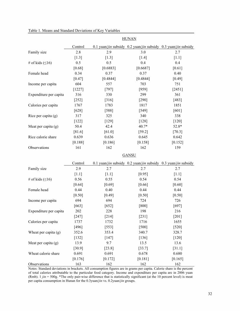
Table 1. Means and Standard Deviations of Key Variables

HUNAN

Control 0.1 yuan/jin subsidy 0.2 yuan/jin subsidy 0.3 yuan/jin subsidyFamily size 2.8 2.9 3.0 2.7 [1.3] [1.3] [1.4] [1.1] # of kids (≤16) 0.5 0.5 0.4 0.4 [0.68] [0.6883] [0.6687] [0.61] Female head 0.34 0.37 0.37 0.40 [0.47] [0.4844] [0.4844] [0.49] Income per capita 604 557 703 751 [1227] [797] [959] [2451] Expenditure per capita 316 330 299 361 [252] [316] [290] [483] Calories per capita 1767 1783 1817 1851 [628] [588] [549] [601] Rice per capita (g) 317 325 340 338 [122] [129] [128] [120] Meat per capita (g) 50.4 42.4 40.7* 52.8* [81.6] [61.0] [59.2] [70.3] Rice calorie share 0.639 0.636 0.645 0.642 [0.188] [0.186] [0.158] [0.152] Observations 161 162 162 159

GANSU

Control 0.1 yuan/jin subsidy 0.2 yuan/jin subsidy 0.3 yuan/jin subsidyFamily size 2.9 2.7 2.7 2.7 [1.1] [1.1] [0.95] [1.1] # of kids (≤16) 0.56 0.55 0.54 0.54 [0.64] [0.69] [0.66] [0.60] Female head 0.44 0.40 0.44 0.44 [0.50] [0.49] [0.50] [0.50] Income per capita 694 694 724 726 [663] [652] [800] [697] Expenditure per capita 202 228 198 216 [247] [214] [231] [201] Calories per capita 1737 1732 1716 1655 [496] [553] [500] [520] Wheat per capita (g) 352.6 353.4 340.7 328.7 [132] [147] [136] [120] Meat per capita (g) 13.9 9.7 13.5 13.6 [30.9] [23.8] [33.7] [31.1] Wheat calorie share 0.691 0.691 0.678 0.680 [0.176] [0.172] [0.181] [0.165] Observations 163 162 162 162 Notes: Standard deviations in brackets. All consumption figures are in grams per capita. Calorie share is the percent of total calories attributable to the particular food category. Income and expenditure per capita are in 2006 yuan (Rmb). 1 jin = 500g. *The only pair-wise difference that is statistically significant (at the 10 percent level) is meat per capita consumption in Hunan for the 0.3yuan/jin vs. 0.2yuan/jin groups.

32

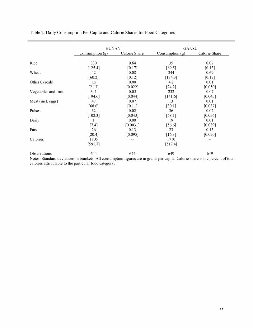
33

Table 2. Daily Consumption Per Capita and Calorie Shares for Food Categories HUNAN GANSU Consumption (g) Calorie Share Consumption (g) Calorie Share Rice 330 0.64 35 0.07 [125.4] [0.17] [69.5] [0.13] Wheat 42 0.08 344 0.69 [60.2] [0.12] [134.3] [0.17] Other Cereals 1.5 0.00 4.2 0.01 [21.3] [0.022] [24.2] [0.050] Vegetables and fruit 341 0.05 232 0.07 [194.6] [0.044] [141.6] [0.045] Meat (incl. eggs) 47 0.07 13 0.01 [68.6] [0.11] [30.1] [0.037] Pulses 62 0.02 36 0.02 [102.3] [0.043] [68.1] [0.056] Dairy 1 0.00 19 0.01 [7.4] [0.0031] [56.6] [0.039] Fats 26 0.13 23 0.13 [20.4] [0.095] [16.3] [0.090] Calories 1805 -- 1710 -- [591.7] [517.4] Observations 644 644 649 649 Notes: Standard deviations in brackets. All consumption figures are in grams per capita. Calorie share is the percent of total calories attributable to the particular food category.

Table 3. Consumption Response to the Price Subsidy: Hunan

(1)

(2)

(3)

(4)

(5)

(6)

(7)

(8)

(9)

Dependent Variable: %Δ Rice Consumption

Dependent Variable: %Δ Meat Consumption

Full Sample

Full Sample

ISCS ≤0.80

ISCS ≤0.80

ISCS >0.80

ISCS >0.80

ISCS 0.60−0.80

Full Sample

Initial Intake >50g

%ΔPrice(rice) 0.224 0.235* 0.451***1 0.466*** -0.61** -0.585** 0.640*** -0.325 -1.125* (0.149) (0.140) (0.170) (0.159) (0.296) (0.262) (0.192) (0.472) (0.625) %Δ Earned 0.043*** 0.047*** 0.024 0.030 0.028 0.105 (0.014) (0.016) (0.023) (0.019) (0.050) (0.069) %ΔUnearned -0.044* -0.038 -0.058 -0.053* 0.061 0.084 (0.025) (0.030) (0.049) (0.030) (0.079) (0.104) %ΔPeople 0.89*** 0.83*** 1.16*** 0.79*** -0.08 0.03 (0.08) (0.09) (0.15) (0.14) (0.27) (0.36) Constant 4.1*** 5.7*** -1.8 0.8 -12.3*** -49.0*** (1.0) (1.1) (1.7) (1.3) (3.1) (3.7) Observations 1258 1258 997 997 261 261 513 997 452 R2 0.08 0.19 0.09 0.20 0.15 0.33 0.24 0.09 0.28 Notes: Regressions are county*time fixed-effect regressions. The dependent variable in columns 1-7 is the arc percent change in household rice consumption and in columns 8-9 it is the arc percent change in household meat consumption. Standard errors clustered at the household level. %ΔPrice(rice) is the change in the subsidy, measured as a percentage of the average price of rice. %ΔEarned is the arc percent change in the household earnings from work; %ΔHH Unearned is the arc percent change in the household income from unearned sources (government payments, pensions, remittances, rent and interest from assets); %ΔPeople is the arc percent change in the number of people living in the household. ISCS (Initial Staple Calorie Share) refers to the share of calories consumed as rice in the pre-intervention period. *Significant at 10 percent level. **Significant at 5 percent level. ***Significant at 1 percent level.

34

Table 4. Robustness of Results to Alternative Specifications: Hunan (1) (2) (3) (4) (5) (6) (7) (8) (9) (10) (11) (12) (13) log-log Specification Consumption Per Capita Individual Level Data Expenditure Per Capita Thresholds Full ≤0.80 >0.80 Full ≤0.80 >0.80 Full ≤0.80 >0.80 ≥25th <25th ≥15th <15th

%ΔPrice(rice) 0.399 0.694** -0.718** 0.762* 1.348*** -1.348 0.233 0.384** -0.223 0.286* 0.139 0.301** -0.132 (0.254) (0.304) (0.294) (0.423) (0.476) (0.842) (0.144) (0.169) (0.225) (0.167) (0.238) (0.153) (0.288) %ΔEarned 0.010** 0.012 0.003 0.091** 0.103** 0.041 0.041*** 0.046*** 0.022 0.039** 0.050** 0.041*** 0.054**

(0.006) (0.007) (0.007) (0.043) (0.048) (0.083) (0.014) (0.016) (0.024) (0.017) (0.023) (0.015) (0.026) %ΔUnearned -0.031** -0.030 -0.038 -0.107 -0.066 -0.225 -0.061** -0.051 -0.082** -0.037 -0.068* -0.033 -0.104**

(0.018) (0.020) (0.025) (0.072) (0.080) (0.174) (0.027) (0.033) (0.041) (0.030) (0.040) (0.028) (0.046) %ΔPeople 0.93*** 0.85*** 1.27*** -0.28 -0.55 0.89 0.01 -0.08 0.27 0.89*** 0.86*** 0.87*** 1.15***

(0.10) (0.10) (0.19) (0.32) (0.35) (0.57) (0.09) (0.10) (0.17) (0.10) (0.15) (0.09) (0.18) Constant 0.04** 0.05** -0.003 11.9*** 16.7*** -5.3 5.3*** 6.5*** 0.8 4.3*** 3.4* 3.9*** 5.4***

(0.02) (0.02) (0.18) (3.0) (3.2) (6.0) (1.0) (1.2) (1.7) (1.1) (1.7) (1.1) (2.0) Observations 1256 997 259 1258 997 261 2755 2191 564 971 287 1083 175 R2 0.11

0.11 0.31

0.09 0.11

0.18 0.05 0.06 0.10 0.18 0.31 0.19 0.35

Notes: Regressions are county*time fixed-effect regressions where the dependent variable is the arc percent change in household rice consumption. Standard errors clustered at the household level. For columns 4 – 13: %ΔPrice(rice) is the change in the subsidy, measured as a percentage of the average price of rice; %ΔEarned is the arc percent change in the household earnings from work; %ΔHH Unearned is the arc percent change in the household income from unearned sources (government payments, pensions, remittances, rent and interest from assets); and %ΔPeople is the arc percent change in the number of people living in the household. For columns 1 – 3, these percent changes result from using the log of the relevant variables. Initial Staple Calorie Share refers to the share of calories consumed as rice in the pre-intervention period. Initial Expenditure Per Capita refers to a household’s percentile in the distribution of expenditure per capita in the pre-intervention period. *Significant at 10 percent level. **Significant at 5 percent level. ***Significant at 1 percent level.

35

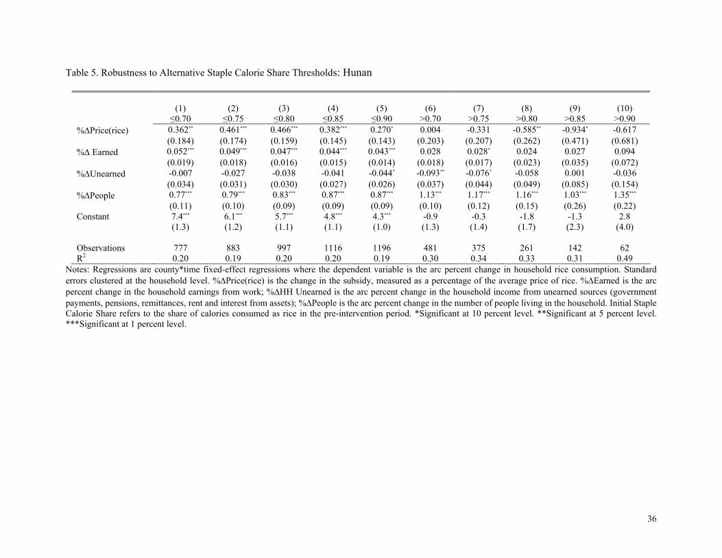
Table 5. Robustness to Alternative Staple Calorie Share Thresholds: Hunan

(1) (2) (3) (4) (5) (6) (7) (8) (9) (10) ≤0.70 ≤0.75 ≤0.80 ≤0.85 ≤0.90 >0.70 >0.75 >0.80 >0.85 >0.90 %ΔPrice(rice) 0.362** 0.461*** 0.466*** 0.382*** 0.270* 0.004 -0.331 -0.585** -0.934* -0.617 (0.184) (0.174) (0.159) (0.145) (0.143) (0.203) (0.207) (0.262) (0.471) (0.681) %Δ Earned 0.052*** 0.049*** 0.047*** 0.044*** 0.043*** 0.028 0.028* 0.024 0.027 0.094 (0.019) (0.018) (0.016) (0.015) (0.014) (0.018) (0.017) (0.023) (0.035) (0.072) %ΔUnearned -0.007 -0.027 -0.038 -0.041 -0.044* -0.093** -0.076* -0.058 0.001 -0.036 (0.034) (0.031) (0.030) (0.027) (0.026) (0.037) (0.044) (0.049) (0.085) (0.154) %ΔPeople 0.77*** 0.79*** 0.83*** 0.87*** 0.87*** 1.13*** 1.17*** 1.16*** 1.03*** 1.35***

(0.11) (0.10) (0.09) (0.09) (0.09) (0.10) (0.12) (0.15) (0.26) (0.22) Constant 7.4*** 6.1*** 5.7*** 4.8*** 4.3*** -0.9 -0.3 -1.8 -1.3 2.8 (1.3) (1.2) (1.1) (1.1) (1.0) (1.3) (1.4) (1.7) (2.3) (4.0) Observations 777 883 997 1116 1196 481 375 261 142 62 R2 0.20 0.19 0.20 0.20 0.19 0.30 0.34 0.33 0.31 0.49

Notes: Regressions are county*time fixed-effect regressions where the dependent variable is the arc percent change in household rice consumption. Standard errors clustered at the household level. %ΔPrice(rice) is the change in the subsidy, measured as a percentage of the average price of rice. %ΔEarned is the arc percent change in the household earnings from work; %ΔHH Unearned is the arc percent change in the household income from unearned sources (government payments, pensions, remittances, rent and interest from assets); %ΔPeople is the arc percent change in the number of people living in the household. Initial Staple Calorie Share refers to the share of calories consumed as rice in the pre-intervention period. *Significant at 10 percent level. **Significant at 5 percent level. ***Significant at 1 percent level.

36

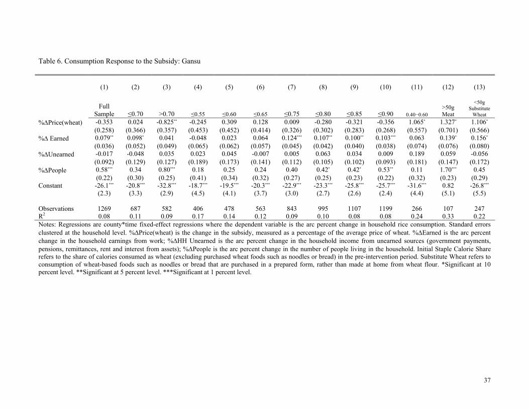
37

Table 6. Consumption Response to the Subsidy: Gansu (1) (2) (3) (4) (5) (6) (7) (8) (9) (10) (11) (12) (13)

Full Sample

≤0.70

>0.70

≤0.55

≤0.60

≤0.65

≤0.75

≤0.80

≤0.85

≤0.90

0.40−0.60

>50g Meat

<50g

Substitute Wheat

%ΔPrice(wheat) -0.353 0.024 -0.825** -0.245 0.309 0.128 0.009 -0.280 -0.321 -0.356 1.065* 1.327* 1.106*

(0.258) (0.366) (0.357) (0.453) (0.452) (0.414) (0.326) (0.302) (0.283) (0.268) (0.557) (0.701) (0.566) %Δ Earned 0.079** 0.098* 0.041 -0.048 0.023 0.064 0.124*** 0.107** 0.100** 0.103*** 0.063 0.139* 0.156*

(0.036) (0.052) (0.049) (0.065) (0.062) (0.057) (0.045) (0.042) (0.040) (0.038) (0.074) (0.076) (0.080) %ΔUnearned -0.017 -0.048 0.035 0.023 0.045 -0.007 0.005 0.063 0.034 0.009 0.189 0.059 -0.056 (0.092) (0.129) (0.127) (0.189) (0.173) (0.141) (0.112) (0.105) (0.102) (0.093) (0.181) (0.147) (0.172) %ΔPeople 0.58*** 0.34 0.80*** 0.18 0.25 0.24 0.40 0.42* 0.42* 0.53** 0.11 1.70*** 0.45 (0.22) (0.30) (0.25) (0.41) (0.34) (0.32) (0.27) (0.25) (0.23) (0.22) (0.32) (0.23) (0.29) Constant -26.1*** -20.8*** -32.8*** -18.7*** -19.5*** -20.3*** -22.9*** -23.3*** -25.8*** -25.7*** -31.6*** 0.82 -26.8***

(2.3) (3.3) (2.9) (4.5) (4.1) (3.7) (3.0) (2.7) (2.6) (2.4) (4.4) (5.1) (5.5) Observations 1269 687 582 406 478 563 843 995 1107 1199 266 107 247 R2 0.08 0.11 0.09 0.17 0.14 0.12 0.09 0.10 0.08 0.08 0.24 0.33 0.22 Notes: Regressions are county*time fixed-effect regressions where the dependent variable is the arc percent change in household rice consumption. Standard errors clustered at the household level. %ΔPrice(wheat) is the change in the subsidy, measured as a percentage of the average price of wheat. %ΔEarned is the arc percent change in the household earnings from work; %ΔHH Unearned is the arc percent change in the household income from unearned sources (government payments, pensions, remittances, rent and interest from assets); %ΔPeople is the arc percent change in the number of people living in the household. Initial Staple Calorie Share refers to the share of calories consumed as wheat (excluding purchased wheat foods such as noodles or bread) in the pre-intervention period. Substitute Wheat refers to consumption of wheat-based foods such as noodles or bread that are purchased in a prepared form, rather than made at home from wheat flour. *Significant at 10 percent level. **Significant at 5 percent level. ***Significant at 1 percent level.

APPENDIX I. UNDERSTANDING GIFFEN BEHAVIOR

Traditionally, the possibility of Giffen behavior has been motivated by an argument

similar to Marshall’s. We will argue that the need to maintain subsistence consumption is the

critical factor leading to Giffen behavior, drawing connections between Marshall’s verbal

argument, two mathematical models of the situation, and the graphical analysis found in

microeconomics textbooks. Although much of what follows in this section has previously

appeared elsewhere, we believe that this analysis provides a useful synthesis of theoretical

approaches to the Giffen phenomenon.

Appendix I.A. The Characteristic-preference Model

We consider very poor consumers whose behavior is driven by the need to achieve a

subsistence calorie intake. Following Lancaster (1966), rather than having preferences over the

foods themselves, we model consumers as having preferences over two fundamental

characteristics of foods: calories, c, and taste, t, where taste is meant to capture the non-nutritive

aspects of food. For expositional ease, we assume there are only two foods, a basic good, b, such

as rice, and a fancy good, f, such as meat. Let (cb, tb) and (cf, tf) denote the calories and taste

provided by a unit of the basic and fancy goods, respectively. Let p > 0 denote the price of the

basic good and normalize the price of the fancy good to 1. Spending one yuan (or Rmb, the

Chinese unit of currency) on the fancy good provides more taste but fewer calories than spending

a yuan on the basic good, i.e., and . /f bc c< p p/f bt t>

The consumer’s first priority is achieving subsistence calorie intake, which we denote by

c*. Once the consumer achieves subsistence, he attempts to maximize the taste of the foods he

eats.45 Since sufficiently impoverished consumers prioritize calories over taste, we begin by

considering a consumer whose objective is to maximize taste subject to budget and subsistence

constraints; later we allow for more general preferences. Let be the consumer’s wealth,

and let b and f denote the units consumed of the basic and fancy goods, respectively. The

consumer chooses b and f to maximize

0w >

b ft b t f+ subject to the budget constraint, pb f w+ ≤ , and

the subsistence constraint, *b fc b c f c+ ≥ .

45 A more general constraint on minimum nutritional requirements behaves similarly.

38

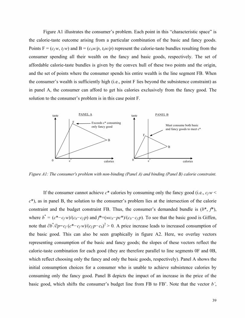
Figure A1 illustrates the consumer’s problem. Each point in this “characteristic space” is

the calorie-taste outcome arising from a particular combination of the basic and fancy goods.

Points F = (cf w, tf w) and B = (cbw/p, tbw/p) represent the calorie-taste bundles resulting from the

consumer spending all their wealth on the fancy and basic goods, respectively. The set of

affordable calorie-taste bundles is given by the convex hull of these two points and the origin,

and the set of points where the consumer spends his entire wealth is the line segment FB. When

the consumer’s wealth is sufficiently high (i.e., point F lies beyond the subsistence constraint) as

in panel A, the consumer can afford to get his calories exclusively from the fancy good. The

solution to the consumer’s problem is in this case point F.

0 0 calories

taste

F

B

c*

PANEL A PANEL B

calories

taste

F

c*

B

Exceeds c* consuming only fancy good Must consume both basic

and fancy goods to meet c*

Figure A1: The consumer's problem with non-binding (Panel A) and binding (Panel B) calorie constraint.

If the consumer cannot achieve c* calories by consuming only the fancy good (i.e., cf w <

c*), as in panel B, the solution to the consumer’s problem lies at the intersection of the calorie

constraint and the budget constraint FB. Thus, the consumer’s demanded bundle is (b*, f*),

where b* = (c*−cf w)/(cb−cf p) and f*=(wcb−pc*)/(cb−cf p). To see that the basic good is Giffen,

note that ∂b*/∂p=cf (c*−cf w)/(cf p−cb)2 > 0. A price increase leads to increased consumption of

the basic good. This can also be seen graphically in figure A2. Here, we overlay vectors

representing consumption of the basic and fancy goods; the slopes of these vectors reflect the

calorie-taste combination for each good (they are therefore parallel to line segments 0F and 0B,

which reflect choosing only the fancy and only the basic goods, respectively). Panel A shows the

initial consumption choices for a consumer who is unable to achieve subsistence calories by

consuming only the fancy good. Panel B depicts the impact of an increase in the price of the

basic good, which shifts the consumer’s budget line from FB to FB’. Note that the vector b’,

39

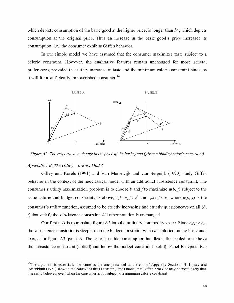
which depicts consumption of the basic good at the higher price, is longer than b*, which depicts

consumption at the original price. Thus an increase in the basic good’s price increases its

consumption, i.e., the consumer exhibits Giffen behavior.

In our simple model we have assumed that the consumer maximizes taste subject to a

calorie constraint. However, the qualitative features remain unchanged for more general

preferences, provided that utility increases in taste and the minimum calorie constraint binds, as

it will for a sufficiently impoverished consumer.46

PANEL A PANEL B

calories

taste

F

B

c* calories

taste F

B

c*

B'

b'

b*

O O

b*

f* f*

f’

Figure A2: The response to a change in the price of the basic good (given a binding calorie constraint)

Appendix I.B. The Gilley – Karels Model

Gilley and Karels (1991) and Van Marrewijk and van Bergeijk (1990) study Giffen

behavior in the context of the neoclassical model with an additional subsistence constraint. The

consumer’s utility maximization problem is to choose b and f to maximize u(b, f) subject to the

same calorie and budget constraints as above, *b fc b c f c+ ≥ and pb f w+ ≤ , where u(b, f) is the

consumer’s utility function, assumed to be strictly increasing and strictly quasiconcave on all (b,

f) that satisfy the subsistence constraint. All other notation is unchanged.

Our first task is to translate figure A2 into the ordinary commodity space. Since cb/p > cf ,

the subsistence constraint is steeper than the budget constraint when b is plotted on the horizontal

axis, as in figure A3, panel A. The set of feasible consumption bundles is the shaded area above

the subsistence constraint (dotted) and below the budget constraint (solid). Panel B depicts two

46The argument is essentially the same as the one presented at the end of Appendix Section I.B. Lipsey and Rosenbluth (1971) show in the context of the Lancaster (1966) model that Giffen behavior may be more likely than originally believed, even when the consumer is not subject to a minimum calorie constraint.

40

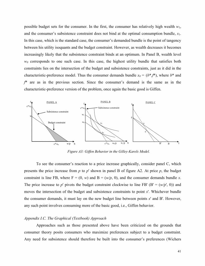
possible budget sets for the consumer. In the first, the consumer has relatively high wealth w1,

and the consumer’s subsistence constraint does not bind at the optimal consumption bundle, x1.

In this case, which is the standard case, the consumer’s demanded bundle is the point of tangency

between his utility isoquants and the budget constraint. However, as wealth decreases it becomes

increasingly likely that the subsistence constraint binds at an optimum. In Panel B, wealth level

w0 corresponds to one such case. In this case, the highest utility bundle that satisfies both

constraints lies on the intersection of the budget and subsistence constraints, just as it did in the

characteristic-preference model. Thus the consumer demands bundle x0 = (b*,f*), where b* and

f* are as in the previous section. Since the consumer’s demand is the same as in the

characteristic-preference version of the problem, once again the basic good is Giffen.

b

f

Budget constraint

Subsistence constraint

w

w/p

c*/cf

c*/cb

PANEL A

b

f

Subsistence constraint

w1

w1/p

c*/cf

c*/cb

x0

x1

w0/p

w0

b

f

F

B

x

x'

B'

PANEL B PANEL C

Figure A3: Giffen Behavior in the Gilley-Karels Model.

To see the consumer’s reaction to a price increase graphically, consider panel C, which

presents the price increase from p to p' shown in panel B of figure A2. At price p, the budget

constraint is line FB, where F = (0, w) and B = (w/p, 0), and the consumer demands bundle x.

The price increase to p' pivots the budget constraint clockwise to line FB' (B' = (w/p', 0)) and

moves the intersection of the budget and subsistence constraints to point x'. Whichever bundle

the consumer demands, it must lay on the new budget line between points x' and B'. However,

any such point involves consuming more of the basic good, i.e., Giffen behavior.

Appendix I.C. The Graphical (Textbook) Approach

Approaches such as those presented above have been criticized on the grounds that

consumer theory posits consumers who maximize preferences subject to a budget constraint.

Any need for subsistence should therefore be built into the consumer’s preferences (Wichers

41

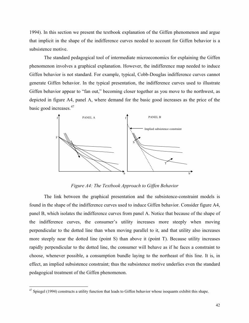
1994). In this section we present the textbook explanation of the Giffen phenomenon and argue

that implicit in the shape of the indifference curves needed to account for Giffen behavior is a

subsistence motive.

The standard pedagogical tool of intermediate microeconomics for explaining the Giffen

phenomenon involves a graphical explanation. However, the indifference map needed to induce

Giffen behavior is not standard. For example, typical, Cobb-Douglas indifference curves cannot

generate Giffen behavior. In the typical presentation, the indifference curves used to illustrate

Giffen behavior appear to “fan out,” becoming closer together as you move to the northwest, as

depicted in figure A4, panel A, where demand for the basic good increases as the price of the

basic good increases.47

b

f

Implied subsistence constraint

T

S

b

f

F

PANEL A PANEL B

Figure A4: The Textbook Approach to Giffen Behavior

The link between the graphical presentation and the subsistence-constraint models is

found in the shape of the indifference curves used to induce Giffen behavior. Consider figure A4,

panel B, which isolates the indifference curves from panel A. Notice that because of the shape of

the indifference curves, the consumer’s utility increases more steeply when moving

perpendicular to the dotted line than when moving parallel to it, and that utility also increases

more steeply near the dotted line (point S) than above it (point T). Because utility increases

rapidly perpendicular to the dotted line, the consumer will behave as if he faces a constraint to

choose, whenever possible, a consumption bundle laying to the northeast of this line. It is, in

effect, an implied subsistence constraint; thus the subsistence motive underlies even the standard

pedagogical treatment of the Giffen phenomenon.

47 Spiegel (1994) constructs a utility function that leads to Giffen behavior whose isoquants exhibit this shape.

42

Thus, despite ostensibly different approaches, the intuition underlying all four

motivations for Giffen behavior is the same. Poor consumers with few substitution possibilities

facing a real or implied subsistence constraint will be forced, following an increase in the price

of a basic good, to consume more of the cheapest source of calories available and less of other

goods. As Gilley and Karels (1991, p.181) note, this suggests that “the most likely place [to find

Giffen behavior] would be among the very poor, consuming a few staples, with limited

substitution possibilities.”

While these factors make detecting Giffen behavior more likely, there is one additional

factor that must be considered. The mechanics of substitution accompanying Giffen behavior

involve the consumer decreasing consumption of more desirable foods such as meat in order to

increase consumption of the staple. However, extremely impoverished consumers may be so

poor that they cannot afford to consume any of the fancy good. In this case, even if the price of

the basic good goes up, Giffen behavior is not possible since there is no good whose

consumption can be reduced to fund increased purchases of the basic good. Thus, while

consumers must be poor, they cannot be too poor.

In light of this, the consumer’s preferences can be thought of as falling into three distinct

zones, as illustrated in figure A5. In panel A, the outer set of indifference curves correspond to

the standard case, where the consumer’s calorie intake is well above subsistence. Over this range

the consumer trades off between calories and taste (and thus between the basic and fancy goods)

in an ordinary way, and thus in panel B they respond to an increase in the price of the basic good

by decreasing consumption of that good. The middle group of indifference curves corresponds to

the range of consumption bundles over which the consumer crosses from malnutrition into

nutritional stability. Over this range, the consumer is willing to sacrifice a great deal of taste (and

thus the fancy good) in order to maintain calories; thus in panel B, they respond to an increase in

the price of the basic good by consuming more of it, i.e., they exhibit Giffen behavior. Finally, in

the inner-most, calorie-deprived zone, the consumer is struggling to achieve subsistence calorie

intake, and therefore values increases in calories almost exclusively. Further, they may be using

their entire budget on only the basic good, and thus as seen in panel B, they have no choice but to

respond to a staple price increase by consuming less of it.

43

Standard Zone

Subsistence Zone

Calorie-Deprived Zone Basic Good

Fancy Good

PANEL A

Standard Zone

Subsistence Zone

Calorie-Deprived Zone Basic Good

Fancy Good

PANEL B

Figure A5. The Different Zones of Consumer Preferences

APPENDIX REFERENCES

Gilley, Otis and Gordon V. Karels (1991). “In Search of Giffen Behavior,” Economic Inquiry, 29(1), p. 182-9.

Lancaster, Kelvin J (1966). “A New Approach to Consumer Theory,” Journal of Political Economy, 74(2), p. 132-157.

Lipsey, Richard G. and Gideon Rosenbluth (1971). “A Contribution to the New Theory of Demand: A Rehabilitation of the Giffen Good,” Canadian Journal of Economics, 4(2), p. 131-163.

Spiegel, Uriel (1994) “The Case of a ‘Giffen Good’,” Journal of Economic Education, c, p. 137–47. van Marrewijk, Charles and Peter A.G. van Bergeijk (1990). “Giffen Goods and the Subsistence Level,”

History of Political Economy, 22(1), p. 145-8. Wichers, Robert (1994) “In Search of Giffen Behavior: Comment,” Economic Inquiry, 32, p. 166-167.

44

APPENDIX II: THE MINIMUM COST DIET AND THE STAPLE CALORIE SHARE

Individual requirements for calories and essential amino acids vary a great deal and depend on a

range of characteristics. To investigate the extent to which it might be possible to judge whether a

particular person was meeting their essential nutritional needs, we solved a simplified version of the “diet

problem,” i.e., minimizing the cost of achieving certain nutritional requirements. To capture the

importance of complete protein sources, using information from the National Research Council we

imposed intake requirements for calories and 11 amino acids.A1 We considered diets consisting of rice

and bean curd in Hunan, and wheat flour and bean curd in Gansu. In both provinces, the staple is the

cheapest source of calories, but it is relatively deficient in the essential amino acid lysine. Complementing

cereal grains with legumes such as in bean curd is typically the cheapest way to ensure that a person

receives all essential amino acids. Typically, only small amounts of bean curd are needed to complete the

protein.

Nutritional content information was taken from the USDA National Nutrient Database for

Standard Reference (the Chinese food tables used in the paper do not contain information on amino acid

content of foods).A2 Calorie requirements are computed using the Estimated Energy Requirement

equations from the Institute of Medicine.A3 In order to capture the realities of cooking technology, we

assume that households receive 13% of their calories from fats, in this case in the form of cooking oil. In

most cases this implies consumption of less than one tablespoon of oil per day.

We considered a number of different representative “people” of both sexes with a range of

different height, weight, and activity level specifications (“V” denotes very active, “A” denotes active,

“L” denotes less active, and “S” denotes sedentary). Scenarios G – J are chosen with typical heights for

Chinese men and women who are slightly underweight or normal weight (by body mass index). For each

person, we solved for the minimum-cost diet that satisfies the nutritional requirements for calories and

each of the essential amino acids. In all cases, the calorie and lysine constraints bind and determine the

solution. Hence to conserve space we do not report the other amino acid requirements.

The results of this exercise show wide variability in both caloric requirements and the cost of the

least-cost diet (see table below). Daily calories required and the least-cost diet range from 1351 calories

and 1.15 yuan/day in Gansu (1.21 in Hunan) for a sedentary elderly woman (scenario E) to 4264 calories

and 2.69 yuan/day in Gansu (2.91 in Hunan) for an active young man (scenario A). Thus the calorie

A1 National Research Council, Dietary Reference Intakes for Energy, Carbohydrates, Fiber, Fat, Fatty Acids, Cholesterol, Protein, And Amino Acids (Dietary Reference Intakes), National Academies Press, Washington DC, 2005. A2 USDA National Nutrient Database for Standard Reference, http://www.nal.usda.gov/fnic/foodcomp/search/. A3 Gerrior, S. et al., “An Easy Approach to Calculating Estimated Energy Requirements,” Preventing Chronic Diesase, 2006, October; 3(4): A129.

45

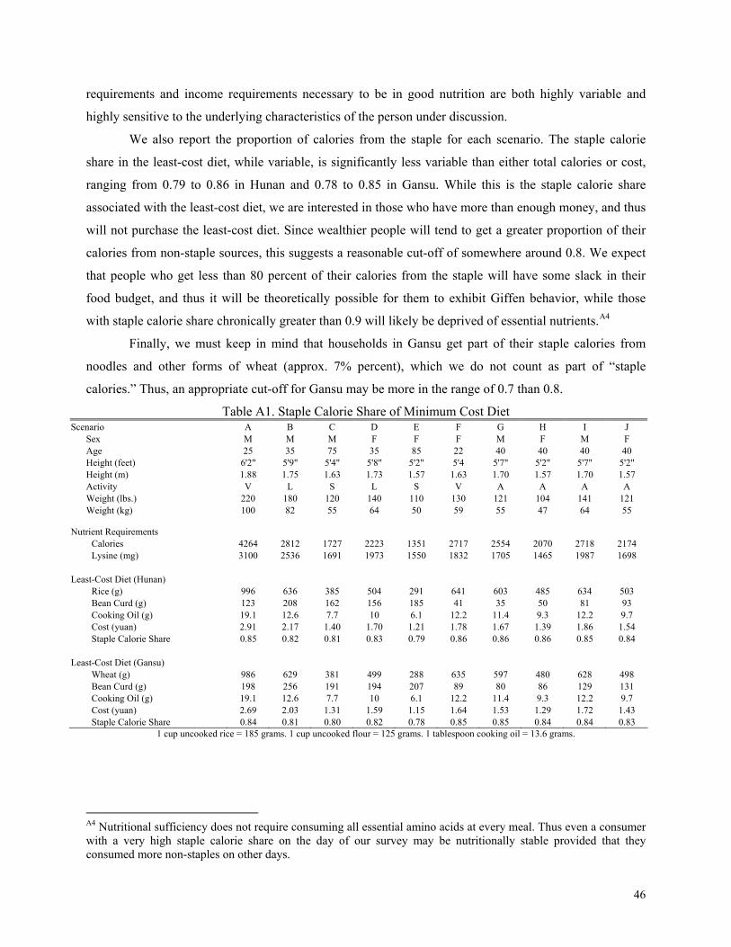
requirements and income requirements necessary to be in good nutrition are both highly variable and

highly sensitive to the underlying characteristics of the person under discussion.

We also report the proportion of calories from the staple for each scenario. The staple calorie

share in the least-cost diet, while variable, is significantly less variable than either total calories or cost,

ranging from 0.79 to 0.86 in Hunan and 0.78 to 0.85 in Gansu. While this is the staple calorie share

associated with the least-cost diet, we are interested in those who have more than enough money, and thus

will not purchase the least-cost diet. Since wealthier people will tend to get a greater proportion of their

calories from non-staple sources, this suggests a reasonable cut-off of somewhere around 0.8. We expect

that people who get less than 80 percent of their calories from the staple will have some slack in their

food budget, and thus it will be theoretically possible for them to exhibit Giffen behavior, while those

with staple calorie share chronically greater than 0.9 will likely be deprived of essential nutrients.A4

Finally, we must keep in mind that households in Gansu get part of their staple calories from

noodles and other forms of wheat (approx. 7% percent), which we do not count as part of “staple

calories.” Thus, an appropriate cut-off for Gansu may be more in the range of 0.7 than 0.8.

Table A1. Staple Calorie Share of Minimum Cost Diet Scenario A B C D E F G H I J

Sex M M M F F F M F M F Age 25 35 75 35 85 22 40 40 40 40 Height (feet) 6'2" 5'9" 5'4" 5'8" 5'2" 5'4 5'7" 5'2" 5'7" 5'2" Height (m) 1.88 1.75 1.63 1.73 1.57 1.63 1.70 1.57 1.70 1.57 Activity V L S L S V A A A A Weight (lbs.) 220 180 120 140 110 130 121 104 141 121 Weight (kg) 100 82 55 64 50 59 55 47 64 55

Nutrient Requirements

Calories 4264 2812 1727 2223 1351 2717 2554 2070 2718 2174 Lysine (mg) 3100 2536 1691 1973 1550 1832 1705 1465 1987 1698

Least-Cost Diet (Hunan)

Rice (g) 996 636 385 504 291 641 603 485 634 503 Bean Curd (g) 123 208 162 156 185 41 35 50 81 93 Cooking Oil (g) 19.1 12.6 7.7 10 6.1 12.2 11.4 9.3 12.2 9.7 Cost (yuan) 2.91 2.17 1.40 1.70 1.21 1.78 1.67 1.39 1.86 1.54 Staple Calorie Share 0.85 0.82 0.81 0.83 0.79 0.86 0.86 0.86 0.85 0.84

Least-Cost Diet (Gansu) Wheat (g) 986 629 381 499 288 635 597 480 628 498 Bean Curd (g) 198 256 191 194 207 89 80 86 129 131 Cooking Oil (g) 19.1 12.6 7.7 10 6.1 12.2 11.4 9.3 12.2 9.7 Cost (yuan) 2.69 2.03 1.31 1.59 1.15 1.64 1.53 1.29 1.72 1.43 Staple Calorie Share 0.84 0.81 0.80 0.82 0.78 0.85 0.85 0.84 0.84 0.83

1 cup uncooked rice = 185 grams. 1 cup uncooked flour = 125 grams. 1 tablespoon cooking oil = 13.6 grams.

A4 Nutritional sufficiency does not require consuming all essential amino acids at every meal. Thus even a consumer with a very high staple calorie share on the day of our survey may be nutritionally stable provided that they consumed more non-staples on other days.

46

APPENDIX III: STAPLE BUDGET SHARE

This section shows results using the initial staple budget share (ISBS) to categorize households

into consumption zones to test for Giffen behavior. As mentioned in the text, we believe the staple calorie

share is the ideal method for identifying consumption zones, both for theoretical reasons and due to

limitations in the expenditure data gathered in our survey. However, intuitively the ISBS captures the

household’s ability to substitute away from luxuries in response to a staple food price change, and is

worth exploring as an alternative. In table A2 below, we show results from estimation of equation (1)

where households are now stratified by whether they spend more than 20 percent of their total budget on

the staple good. For Hunan, the results again suggest that the poorest households are Giffen consumers.

Consistent with expectations, the elasticity is smaller for wealthier households, though the point estimate

is positive and we can’t reject that they also are Giffen consumers (or that the elasticity is the same as for

the poorer households). For Gansu, the same broad pattern also fits, with a much greater coefficient for

the poorest households, though in this case both point estimates are negative.

We can explore the demand elasticity-budget share relationship in more detail by examining the

coefficient plots, as in figure 2 in the main text. In figure A6 below, the inverted-U pattern of the

elasticities is again strongly evident for Hunan. The elasticity is large and positive for households in the

middle range of ISBS, i.e., households that are poor-but-not-too-poor. The elasticity then declines towards

zero for both poorer and wealthier households. However, the coefficients never become statistically

significantly negative. For Gansu, there is no evidence of an inverted-U shaped pattern of elasticities, with

the curve largely negative and declining over much of the range of ISBS. However, as stated in the main

text, our predictions for household consumption patterns may fail because on average, households in

Gansu do not satisfy the conditions of the basic set up we described. Therefore, in the bottom panel of the

figure, we condition on households consuming at least 50 grams of meat. Under these conditions, a clear

inverted-U shaped pattern emerges, with statistically significant Giffen behavior over a middle range of

ISBS, with declining elasticities for both wealthier and poorer households. However, as with Hunan, the

elasticities do not become statistically significantly negative for the poorest or wealthiest households. But

overall, for both Hunan and Gansu, with this alternative measure we again find statistically significant

evidence of Giffen behavior for a range of consumers, and an inverted-U shaped pattern of elasticities.

However, as anticipated, the ISBS does not as accurately segregate households into different

consumptions zones as ISCS.

47

Table A2. Consumption Response to the Price Subsidy: Initial Staple Budget Share

HUNAN GANSU (1) (2) (3) (4) ISBS ≤.20 ISBS >.20 ISBS ≤.20 ISBS >.20 %ΔPrice(rice/wheat) 0.275* 0.144 -0.184 -1.067** (0.154) (0.301) (0.288) (0.511) %Δ Earned 0.049*** 0.014 0.122*** -0.099 (0.016) (0.022) (0.041) (0.072) %ΔUnearned -0.052* 0.013 -0.024 0.066 (0.029) (0.049) (0.105) (0.170) %ΔPeople 0.86*** 1.32*** 0.52** 0.88** (0.09) (0.18) (0.25) (0.44) Constant 5.1*** -1.5*** -24.7*** -30.7*** (1.1) (2.1) (2.6) (4.9) Observations 1059 199 1062 207 R2 0.19 0.30 0.07 0.18 Notes: Regressions are county*time fixed-effect regressions. The dependent variable is the arc percent change in household rice (Hunan) or wheat (Gansu) consumption. Standard errors clustered at the household level. %ΔPrice(rice/wheat) is the change in the subsidy, measured as a percentage of the average price of rice/wheat. %ΔEarned is the arc percent change in the household earnings from work; %ΔHH Unearned is the arc percent change in the household income from unearned sources (government payments, pensions, remittances, rent and interest from assets); %ΔPeople is the arc percent change in the number of people living in the household. ISBS (Initial Staple Budget Share) refers to the share of the total household budget devoted to the staple good in the pre-intervention period. *Significant at 10 percent level. **Significant at 5 percent level. ***Significant at 1 percent level.

-2-1

01

2

0 .05 .1 .15 .2 .25 .3Household Staple Budget Share

-2-1

01

2

0 .05 .1 .15 .2 .25 .3Household Staple Budget Share

HUNAN GANSU

-5-4

-3-2

-10

12

34

5

0 .05 .1 .15 .2Household Staple Budget Share

GANSU >50g meat

Figure A6: Coefficient Plots

48

APPENDIX IV. CALCULATING VOUCHER USE TO EXAMINE POTENTIAL CASHING OUT

An ideal measure of whether households had cashed out vouchers would compare, for

each household, the total number of vouchers redeemed over the course of the intervention with

the total amount of the staple consumed by the household and any increase in storage of the

staple. However, this measure is simply not feasible since it would require continuously

observing both variables for the whole period.48 Since our consumption data is based on only

single-day observations on the survey dates, our estimate of total consumption over the subsidy

period is imprecise.49 In addition, while we attempted to collect data on storage, response rates

for the storage questions were very low because of respondents’ difficulties in interpreting the

questions. As a result, while these data can provide broad guidance in understanding the

implementation of the intervention, the inherent imprecision associated with these measures is

quite high. Nevertheless, for the sake of completeness we present approximate calculations.

Each household was issued vouchers sufficient to purchase 750g of the staple per person

per day. This corresponds to vouchers sufficient to purchase (on average) 2106 grams per day of

rice for a typical household in Hunan. Overall, only 51% of vouchers that had been distributed as

of the second survey had actually been redeemed by that time, meaning that the average

household had redeemed the equivalent of 1078 grams per day.50 Estimated daily rice

consumption for subsidized households during the subsidy period was 955 grams, implying a

residual difference of 123 grams of rice per household per day, or 10% of the total number of

vouchers redeemed before the second round of the intervention. However, as stated, it is likely

that households used the subsidy to stock up on rice for later consumption. While our storage

data are limited, we find that on average, household rice stores increased from 0.6 jin to 14.5

jin,51 which corresponds to redeeming an additional 74g of vouchers per household per day,

48 Further, due to administrative difficulties in assigning and recovering individual identifiers from the vouchers, we unfortunately have only data on aggregate voucher usage to work with. 49 And there is evidence of seasonality in consumption, especially for wheat in Gansu, with the control groups in each county displaying a decline in consumption between rounds 1 and 2. Thus, in estimating the consumption of subsidy households during the subsidy period, we need to take into consideration that the round 2 consumption will be an underestimate of the consumption during a typical day of the subsidy period. To correct for this, we take the change in average consumption between rounds 1 and 2 for the control group in each county, assume a linear trend in consumption, and use this to adjust the round 2 consumption estimates for the treatment group. 50 Overall, 76% of all vouchers issued were redeemed; as expected, there was a substantial increase in voucher redemption as the subsidy period drew to a close. 51 Due to low response rates (19% in round 2) we base this calculation only on households that responded to the storage question in both the first and second rounds of the survey.

49

accounting for much of the discrepancy between rice consumed and vouchers redeemed. And

observations by our survey teams corroborate that households were, in fact, increasing storage

during this time. Thus, as a rough approximation, only 3%52 more vouchers were redeemed than

were consumed or stored,53 suggesting that if there were any cashing out or re-selling, it was

extremely limited.54

In Gansu, a typical household received 1996 grams of vouchers per day, and only 46% of

vouchers available before the second-round survey were redeemed before that survey. Average

household wheat intake in the first two rounds of the survey was 747g, while approximately

942g worth of vouchers per day were redeemed, for a difference of 195g per household per day.

There is also evidence of increased storage in Gansu, which accounts for approximately 72g of

additional voucher usage per day, leaving approximately 123g (about 1 cup) of voucher

redemptions unaccounted for, and a net-of-storage excess voucher redemption rate of 11%.55

There are in particular two counties in Gansu that account for much of the discrepancy;

Kongdong (35% unaccounted for vouchers) and Anding (22%). We discovered that the high rate

of voucher redemptions in Anding was due to the implementation team departing from our

protocol and explicitly advising households to purchase as much wheat as possible and store it in

order to take advantage of the subsidy program.56 And the implementation team reports that

households were, in fact, purchasing and storing a great deal of extra wheat in Anding (given the

imperfections in our storage data, it would not be surprising if we did not measure this increase).

We have been unable to uncover the reason for the high voucher redemption rate in Kongdong,

although our ground personnel report high storage levels and little evidence of cashing out of

vouchers.57 While we have no direct evidence of cheating in these counties and the high

52 While estimates at the county level are less precise, the only real outlier, with 217g grams or 10% more vouchers redeemed than can be accounted for by consumption and storage is Pingjiang county. To the extent that we view this as an outlier, the results of table 4 are robust to removing this county. 53 Further, there may be additional ‘leakage’ our survey doesn’t capture, such as consumption by visitors to the household, or rice lost or wasted during the cooking process, which may further explain the remaining discrepancy. 54 While it is possible that households cashed out vouchers and then inflated their reported rice consumption to hide what they had done, this type of sophisticated cheating would work against our finding Giffen behavior. 55 It is likely that in Gansu leakage is somewhat higher than in Hunan since flour is frequently used incidentally in the cooking process (e.g., covering surfaces for kneading bread) in ways that may not appear in the intake data. 56 To the extent that this advice encourages households to reduce consumption expenditure today in order to purchase and store wheat, this might work against our finding of Giffen behavior since when households spend less on current consumption they tend to consume relatively more wheat. 57 In fact, both counties show large increases in reported wheat purchases between the first and second round of the survey (despite there being a 40% across-the-board decline in wheat consumption and all other counties reporting reduced purchases). Reported purchases match up well with voucher usage in Anding and Kongdong.

50

redemption rates were apparently due to increasing wheat storage, as an additional robustness

check we estimated regression (1) for Gansu under two scenarios. The first excludes just

Kongdong, for which we have no clear reason for the discrepancy. Doing so, the resulting

elasticity estimate for the 0.4 - 0.6 staple-calorie share group actually increases in both

magnitude and statistical significance (1.37 (.67)) relative to the results using all counties (1.06

(0.56)). Excluding both Anding and Kongdong, which reduces the sample size by 42%, results in

an elasticity estimate of 0.79 with a p-value of 0.27. Thus, while the elasticity estimate remains

positive, it is no longer statistically significant.58

58 Running the main regression in equation (1) with interactions for whether the household was a treated household in Anding or Kongdong, we are unable to reject the null hypothesis that these counties are the same as the other Gansu counties. For this reason, we have not eliminated them from the regressions reported in tables 7 and 8.

51