NBER WORKING PAPER SERIES

MEASURING THE WELL-BEING OF THE POORUSING INCOME AND CONSUMPTION

Bruce D. MeyerJames X. Sullivan

Working Paper 9760http://www.nber.org/papers/w9760

NATIONAL BUREAU OF ECONOMIC RESEARCH1050 Massachusetts Avenue

Cambridge, MA 02138June 2003

This paper was prepared for the Joint IRP/ERS Conference on Income Volatility and Implications for FoodAssistance, May 2-3, 2002 in Washington, DC. We thank seminar participants at the University of Colorado,the ERS, the University of Illinois at Chicago, the University of Notre Dame, the NBER Labor Studies andConsumer Expenditure Survey meetings, and Northwestern University for their comments, and John Bound,Charlie Brown, Angus Deaton, Thesia Garner, Jonathan Gruber, Dean Jolliffe, Joseph Lupton, Bruce Spencer,Frank Stafford and Robert Van Horn for suggestions. The views expressed herein are those of the authors andnot necessarily those of the National Bureau of Economic Research.

©2003 by Bruce D. Meyer and James X. Sullivan. All rights reserved. Short sections of text not to exceedtwo paragraphs, may be quoted without explicit permission provided that full credit including © notice, isgiven to the source.

Measuring the Well-Being of the Poor Using Income and ConsumptionBruce D. Meyer and James X. SullivanNBER Working Paper No. 9760June 2003JEL No. D12, I32

ABSTRACT

We evaluate consumption and income measures of the material well-being of the poor. We begin

with conceptual and pragmatic reasons that favor income or consumption. Then, we empirically

examine the quality of standard data by studying measurement error and under-reporting, and by

comparing micro-data from standard surveys to administrative micro-data and aggregates. We also

compare low reports of income and consumption to other measures of hardship and well-being. The

closer link between consumption and well-being and its better measurement favors the use of

consumption when setting benefits and evaluating transfer programs. However, income retains its

convenience for determining program eligibility.

Bruce D. Meyer James X. SullivanDepartment of Economics University of Notre DameNorthwestern University Department of Economics2003 Sheridan Road 447 Flanner HallEvanston, IL 60208 Notre Dame, IN 46556and NBER Sullivan.197@nd.edubmeyer@northwestern.edu

1 An exception is Mathiowetz, Brown, and Bound (2002).

2 World Bank (2001) summarizes this preference for consumption measures of poverty. Forexample, on page 17 the report argues that “Consumption is conventionally viewed as thepreferred welfare indicator, for practical reasons of reliability and because consumption isthought to better capture long-run welfare levels than current income.” See Deaton (1997),particularly Section 1.2, for an informative discussion of income and consumption measurementissues in developing countries. For a paper that argues for the use of income in developedcountries see Atkinson (1991).

I. Introduction

Income is almost exclusively used to measure economic deprivation in the United States.

Relative to consumption, income is generally easier to report and is available for much larger

samples, providing greater power to test hypotheses. An extensive literature examines the

effects of low income on child outcomes such as test scores, behavior problems, and health (for

example, see Mayer 1997). While the accuracy of income reports in many datasets has been

analyzed, this work has not focused on validating income measures for poor families.1 For those

at the bottom, where the extent of material deprivation is most important, there is little evidence

to support the reliability of income measures. Moreover, there is significant evidence suggesting

that income is badly measured for the poor.

Unlike the U.S., in developing countries consumption is the standard measure of material

well-being.2 While there are obvious differences between developing and developed countries,

such as the extent of formal employment, these distinctions are blurred when looking at the poor

in developed countries who may do little formal work. Arguably, consumption is better

measured than income for poor families. Consumption is less vulnerable to under-reporting bias,

and ethnographic research on poor households in the U.S. suggests that consumption is better

2

reported than income. There are also conceptual and economic reasons to prefer consumption to

income because consumption is a more direct measure of material well-being.

This paper examines the quality of income and consumption measures of material

well-being. We explore both conceptual and measurement issues, and compare income and

consumption measures to other measures of hardship or material well-being. Our analysis

begins by exploring the conceptual and pragmatic reasons why consumption might be better or

worse than income. We then consider five empirical strategies to examine the quality of income

and consumption data. First, we compare the income and consumption reports, along with assets

and liabilities, for those with few resources to examine evidence of measurement error and

under-reporting. Second, we investigate other evidence on the internal consistency of reports of

low income or consumption. Third, we compare how well micro-data in standard datasets

weight up to match aggregates for classes of income and consumption that are especially

important for low-resource families. Fourth, we examine comparisons of household survey

reports of transfer receipt to administrative micro-data on transfer receipt. Fifth, we evaluate

income and consumption measures by comparing them to other measures of hardship or material

well-being.

We find substantial evidence that consumption is better measured than income for those

with few resources. We also find that consumption performs better as an indicator of low

material well-being. These findings favor the examination of consumption data when policy

makers are deciding on appropriate benefit amounts for programs such as Food Stamps, just as

consumption standards were behind the original setting of the poverty line. Similarly, the results

favor using consumption measures to evaluate the effectiveness of transfer programs and general

3 Haig and Simons (Rosen 2002) provide a conceptually better measure of income defined as thenet increase in the ability to consume during a period. In other words, consumption plus netadditions to wealth. This definition would include unrealized capital gains, the flow value ofdurable services, employer provided fringe benefits, and other items. Such a definition cannotbe implemented with conventional survey data.

3

trends in poverty and food spending. Nevertheless, the ease of reporting income favors its use as

the main eligibility criteria for transfer programs such as Food Stamps and Temporary

Assistance for Needy Families (TANF).

II. An Analytical Framework for Income and Consumption Data

There are both conceptual and reporting reasons why one might prefer either

consumption or income data when examining the level of or changes in the material well-being

of the most disadvantaged families. The conceptual issues strongly favor consumption, while

reporting issues tend to favor income for most people but not for low-resource populations.

To make these ideas as precise as possible, we first need to define income, consumption,

and expenditures. We define income (what might be better called survey income) as the inflow

of money and near money to a family. Because we want to reflect consumable resources, we

subtract taxes on income and add the face value of Food Stamps, which are close to money in

practice. One should note that this definition reflects what one can potentially measure well in a

household survey rather than a Haig-Simons type measure.3

Expenditures is the outflow of money from a household. Consumption starts from

expenditures but replaces the outlays for durable goods with the flow value of services from

these goods (this adjustment is feasible for housing and cars in our data), minus expenditures on

4 For further discussion see Cutler and Katz (1991), Slesnick (1993), or Poterba (1991).5 Poterba (1991) provides evidence that the difference between current income and currentexpenditures is larger for very young and very old households, suggesting that some of thisdisparity is likely the result of life-cycle behavior, and that current income understates well-being for these households. See Blundell and Preston (1998) for a recent formal analysis ofthese issues and the potential for combining income and consumption data.

4

investment items (medical care, education) minus cash gifts to other families and charities.

In practice, survey income, expenditures, and consumption are all measured with

significant error. Thus we can write observed income, expenditures and consumption as

Y=Y*+εY, E=E*+εE, and C=C*+εC, where Y*, E*, and C* are the true values of these concepts,

and εY, εE, and εC are the corresponding errors in the observed values. The conceptual reasons to

prefer income or consumption deal with differences between Y*, E*, and C*, while the reporting

reasons deal with the distributions of εY, εE, and εC .

A. Conceptual Issues

Economic theory suggests that current consumption more directly measures the material

well-being of the family than current income.4 Current income can be a misleading indicator of

the economic status of the family because earnings are susceptible to temporary fluctuations due

to transitory events such as layoffs or changes in family status. These temporary changes cause

current income to vary more than consumption, but they do not necessarily reflect changes in

well-being (for example, see Wemmerus and Porter 1996). Consumption is more likely to

capture a family’s long-term prospects than is income.5 Income measures also fail to capture

disparities in consumption that result from differences across families in the accumulation of

assets or access to credit (Cutler and Katz 1991). Expenditures reflect a family’s long-term

5

prospects but may be lumpy because of the indivisibility of certain purchases such as houses and

cars. Consumption though should reflect the smoothed flow of services obtained from these

durable goods.

The insurance value that means-tested transfer programs provide for both recipients and

potential recipients is likely to change as reforms alter program generosity and eligibility.

Consumption is more likely to reflect these changes in insurance values than is income, though

not in all cases. For example, if welfare is a valuable source of insurance for poor families, then

the value of this insurance falls as welfare reform introduces more rigid eligibility rules such as

time limits and work requirements. This change creates an incentive for these families to find

alternative sources of insurance such as increased savings, resulting in reduced consumption,

holding income fixed. Alternatively, families could choose to increase earnings by working

more. However, in this case, an income measure of material well-being would suggest that

families are better off as a result of the reduction in insurance. However, one should note that a

single year’s consumption or income may often be a poor proxy for inter-temporal utility. It is

possible to construct situations where inter-temporal utility and income rise, while consumption

falls.

So far, these arguments that suggest consumption better captures material well-being than

income rely on differences between Y* and C* that are due to savings. For the low-educated

single mother population on which we focus, we believe that Y* and E* are in most cases the

same because little saving and dissaving occurs for this group. Nevertheless, C* differs from Y*

due to the differences between expenditures on durables and the service flow from them.

In addition, income does not reflect in-kind transfers, such as Medicaid, that are reflected

6

in expenditure data. These in-kind transfers are a particularly important source of support for

families with low cash incomes. Recent changes in Medicaid and SCHIP are likely to

substantially affect family well-being without affecting measured family income. On the other

hand, non-medical consumption measures would reflect the Medicaid changes. If single mothers

spend less out of pocket on health care, they can spend more on food and housing.

That consumption can be divided into meaningful categories such as food and housing

provides two advantages over income. First, one can directly measure well-being using essential

expenditure categories such as food and housing, and one can measure child well-being using

child clothing and other child goods. Second, one cannot account for relative price changes with

a single deflator for income. However, one can deflate different components of consumption

using different price indices. This flexibility may be particularly important if the market basket

of goods consumed by those with few resources differs from the general population.

Income measures may also fail to handle appropriately illegal activity. For example, if

the illicit activity is on the expenditure side (drug purchases for example), expenditures on food,

housing, or total expenditures (which do not include illicit drug purchases) would still provide

meaningful summary information on family well-being. In the case of an individual selling

illicit drugs, this individual may not report revenue from this illicit activity as income (a problem

for income data), but involvement in illicit activity does not imply that food and housing

expenditures will be mis-reported. This second case is really an example of why the absolute

value of the error in reported income, εY, might be much larger than the error in reported

consumption, εC, which is the issue on which the next sub-section focuses.

6This finding is for a very select subset of observations that can be matched in the CPS andSocial Security earnings records with non-truncated, non-imputed earnings in coveredemployment.

7

B. Reporting Issues

While there are conceptual reasons to prefer consumption to income, the extent to which

income and consumption are reported with error is the other main issue in choosing a measure of

material well-being. We believe that the main reason to prefer consumption to income is that

measurement error in consumption is less pronounced for those with few resources than is

measurement error in income.

First, we should mention the key reason why income is generally more used than

consumption: income is often easier to report. Income is particularly easy to report when it

comes from one source and is recorded on a W-2 received in the mail which is in-turn entered on

a tax form submitted to the IRS. Finding by Bound and Krueger (1991) support the idea that

income is easy to report-- more than 40 percent of Current Population Survey (CPS) respondents

report earnings that are within 2.5 percent of IRS earnings.6 This argument is probably the main

reason most surveys rely on income measures and is pursuasive for many demographic groups.

However, for some demographic groups that are particularly important from a poverty

and public policy perspective, such as low-educated single mothers, this argument is not

compelling. For low-educated single mothers, income often comes from many other sources

besides earnings in formal employment. For these disadvantaged families, transfer income

(which is consistently under-reported in surveys) and off-the-books income (which is likely to be

unreported in surveys) account for a greater fraction of total income. For example, in the welfare

8

reliant single mother sample in Edin and Lein (1997), the average single mother obtains at least

ten percent of her income from each of four different sources (Aid to Families with Dependent

Children (AFDC), Food Stamps, unreported work, boy friends/absent fathers) and only two

percent from reported work. With many sources of income that do not appear on a W-2

statement, accurate reporting is much less likely.

Furthermore, tax payments are often not reported in household surveys. Taxes can be

imputed, but there is error in this process. Thus, even if pre-tax income is typically recorded

precisely, after-tax income is usually not. On the other hand, consumption already reflects net of

tax resources. Since tax credits can be a forty percent addition to earned income for low-income

parents, accounting for taxes is essential to properly measure material well-being.

While most families may be able to report the amount they earn (at least pre-tax) with

greater accuracy than the amount they spend on goods and services, this argument is less

compelling for groups that spend a large fraction of their resources on food and housing.

Furthermore, the consumption of food and housing may be of interest in their own right and

sufficient statistics for well-being if their share of the budget is fairly similar across families,

once one controls for total expenditures. Food and housing together constitute nearly 70 percent

of the consumption of low-educated single mothers and thus provide a reasonable measure of

material well-being.

Another advantage of income surveys is that they tend to have larger sample sizes and

thus greater precision. Because consumption data are much more costly to collect for a given

sample size, datasets with consumption information are much smaller. The larger samples with

income data allow patterns to be determined with greater precision, analyses of subsamples to be

9

performed with confidence, and hypotheses to be tested with greater power. Furthermore,

income measures are available in many datasets that include other variables of interest.

Nevertheless, evidence suggests that the gain in precision from using income is not as great as a

simple comparison of sample sizes suggests (Meyer and Sullivan, Forthcoming).

While ease of reporting and precision may favor income, for low-resource families

income is often subject to substantial under-reporting. Overall, it appears that income is under-

reported, and evidence shows that specific types of income such as self-employment earnings,

private transfers, and public transfers are under-reported. Part of the explanation for this finding

is that income seems to be a more sensitive topic and easier to hide. An additional issue is that

income under-reporting has increased, making time-series comparisons problematic. We now

discuss these issues in turn.

Research looking at both family income and consumption shows that reported income

falls well short of reported consumption. Cutler and Katz (1991) note that the fraction of

individuals with income below the poverty line is much larger than the fraction with

consumption below the poverty line. Slesnick (1993) also emphasizes that poverty rates based

on total expenditures are much lower than those based on income. Several papers have pointed

out that the reported expenditures of those who report low incomes often are multiples of their

reported incomes (Rogers and Gray 1994; Jencks 1997; Sabelhaus and Groen 2000). We discuss

these issues more in Section IV.

Self-employment tends to be concentrated at the top or the bottom of the income

distribution. Under-reporting of income is of particular concern for the self-employed, so this

problem may be worse for assessing the well-being of the poor. Reported income tends to miss

7 Consumption will also miss some in-kind transfers, but the consumption measure we useincludes the service flow from gifts of cars, and will incorporate some gifts of housing or rent.

10

monetary transfers from family and friends as well as in-kind transfers.7 In-depth interviews in

ethnographic research have shown that a large share of low-resource single mothers obtain

substantial income in transfers from family and friends, boyfriends, and absent fathers (Edin and

Lein 1997). These transfers typically are not captured in survey data on income.

In addition to the under-reporting of earnings and private transfers, household surveys

also fail to capture the full value of government transfers, particularly for single mothers. Coder

and Scoon-Rogers (1996) and Roemer (2000) have documented the pattern of under-reporting

for a large number of transfer programs (see Hotz and Scholz (2002) and Moore et al. (1997) for

recent reviews). There are also many studies that focus on under-reporting in a few programs or

a single transfer program such as Bavier (1999) and Primus et al. (1999) on AFDC/TANF and

Food Stamps. Bollinger and David (1997, 2001) examine Food Stamps, Bitler, Currie, and

Scholz (2003) study WIC and Food Stamps, and Giannarelli and Wheaton (2000) and Meyer

(2002) examine SSI. Another strand of the evidence comes from micro-validation studies such

as Marquis and Moore (1990) and Moore, Marquis, and Bogen (1996). We will discuss these

issues at length in Section IV.

A view among some researchers is that individuals are more willing to report their

expenditures than their income, possibly because they are primarily taxed on their income rather

than their expenditures. This view is certainly consistent with the high rates of non-response in

the CPS that are listed in Table 3 of Moore et al. (1997). They report non-response rates of over

twenty-five percent for most of the large income categories, on top of the 7-8 percent interview

8 Mayer and Jencks (1993) provide evidence for an earlier period that the growth in both means-tested transfers and illegitimate income resulted in an increase in the under-reporting of income.

11

refusal rate. For example, in 1996 the non-response rate was 26.2 percent for wage and salary

income, 44.1 percent for interest income, and 30.2 for pension income. The reason for non-

response is generally that the interviewee refused to answer or indicated that he/she did not know

the answer. In the Consumer Expenditure Survey (CE) the interview non-response rate was 17

percent, and in a typical year about 9 percent of expenditure categories are imputed, totaling

about 13 percent of total expenditures. Thus, the fraction of households with missing or imputed

expenditure data is quite a bit lower in the CE than in the most used income data source.

Changes in the extent of under-reporting over time exacerbates the problem of

understated income (see Meyer and Sullivan, Forthcoming, for an extended discussion of this

issue). For example, a diminished dependence on cash transfers, which have high implicit tax

rates, reduces the incentive to hide income. AFDC caseloads fell dramatically after March of

1994, reducing the incentive for single mothers to hide income. Consequently, reported income

for these families might rise even if the true value of income does not change.8 Recent Earned

Income Tax Credit (EITC) expansions also changed the incentives to under-report income by

increasing the incentive to substitute on-the-books earnings (which would be partially matched

by credit dollars) for off-the-books income.

Under-reporting of means-tested cash transfers (AFDC/TANF and Food Stamps) has

increased in recent years (Bavier 1999; Primus et al. 1999). Overall, unreported cash transfers

grew by 68 percent from 1993 to 1997. Assuming poor families under-report these transfers at

the same rate as all welfare recipients, this rise in under-reporting alone would bias downward

9 This figure is based on the authors’ calculations using CPS and administrative data reported inBavier (1999).

12

measured changes over this period in income for single mothers in the bottom income quintile by

nearly 8 percentage points.9 Even if under-reporting rates were not changing, the dramatic

changes in transfer and tax programs in recent years would still lead to large changes in biases

over time.

Overall, there is substantial evidence to indicate that |εY| is often large and that εY is

much more likely to be a large negative number than a large positive one. Certainly,

consumption is measured with error as well. However, families do not have the same incentives

to under-report consumption, so there is little reason to suspect that the rate at which families

mis-report consumption has changed over time. Moreover, under-reporting of consumption is

not likely to be correlated with policy changes. Because the evidence shows that reported

consumption often exceeds income for those with few resources, one might be concerned that

consumption is systematically over-reported–an issue discussed in Section IV.

III. Data and Methods

We examine measures of material well-being from several sources including the

Consumer Expenditure Survey (CE), the Panel Study of Income Dynamics (PSID), and the

March Current Population Survey (CPS). This section provides a brief description of the

samples drawn from these nationally representative datasets for our analysis and outlines how

we construct measures of consumption, expenditures, and income. Appendix 1 provides a more

10 The March CPS does not include data on expenditures. Limited data on food expenditures areavailable in the CPS Food Security Supplement, which was first administered in April of 1995.

13

detailed description of these datasets as well as definitions for our measures of material well-

being.

Of the two data sources that provide both expenditure and income data for the same

families–the CE and the PSID–the CE offers more extensive information on family expenditures,

while the PSID offers high quality data on family income.10 The Interview Survey of the CE is a

rotating panel survey of approximately 5,000 households each quarter, interviewing each

household for up to five consecutive quarters. This survey provides comprehensive data on

household level expenditures. From the quarterly interview, information on spending for about

600 unique expenditure categories is provided. The Interview Survey also provides data on

family earnings, transfer income, and tax liabilities. These data are derived from questions

covering about 30 different components of income and taxes. These income and tax questions

are asked of each member of the family over the age of 14.

Although the PSID does not provide data on total household expenditures, in most years

respondents report spending for food at home and food away from home, as well as the dollar

value of Food Stamps received. The survey also includes approximately 30 questions about

housing arrangements and housing costs. The PSID income data are widely considered to be

among the best available (Kim and Stafford 2000). These data include more than 250 income

and tax variables derived from a very detailed list of questions about family income. These

variables include separate income information for the head, the spouse, and other family

members.

11 This poverty rate is based on the authors’ calculations using the official definition of povertyfrom the U.S. Census and a sample of low-educated single mothers in the CPS from 1992-1999. Sixty percent of this sample have reported consumption levels that fall below the official povertythreshold. 12 This figure is based on the authors' calculations using data from the 1999 March CPS.

14

In addition to annual measures of family income, inter-family transfers, and food and

housing expenditure data, the PSID provides a detailed inventory of the family’s asset and

liability portfolio at five-year intervals (1984, 1989, 1994, and 1999). Data on all of these

elements of the family budget constraint enable us to examine more directly how families

balance their budgets.

We focus on families that are likely to be disadvantaged given their demographic

characteristics, rather than restricting attention to families that report limited resources, because

the latter approach will systematically bias comparisons of income and consumption by

conditioning on the variables under study. To avoid stacking the deck against either income or

consumption, we focus on families headed by a single mother without a high school degree as an

easily definable group that typically has very limited resources–more than three-quarters of these

families fall below the poverty line.11 Many of these families benefit from government transfer

programs. On average Food Stamps, TANF, and SSI account for about a third of total income for

low-educated single mothers.12 More than half of all single mothers without a high school degree

were on welfare in a typical year prior to recent welfare reforms. Although our results and much

of our discussion focus on low-educated single mothers, for some of our analyses we also

examine other disadvantaged groups including the disabled and the aged poor. These groups also

receive substantial government transfers so their income is not largely reported on a W-2.

Finally, we also examine more broadly defined samples, including a sample of all single mother

13 We constructed family units in the PSID and the CPS in order to most closely match thedefinition of single mother families as defined by the CE: “One parent, female, own childrenonly, at least one child age under 18 years old.” See Appendix 1 for more details.14 In particular, we use a scale factor equal to s/(mean of s), where s= 1/(number of adults +number of children*0.7)0.7. This is a fairly standard equivalence scale that follows NationalResearch Council (1995).

15

families as well as a sample of all U.S. families, in order to demonstrate that our results are not

limited to a few narrowly defined demographic groups.

From each dataset we construct samples of families headed by a single woman between

the ages of 18 and 54 who does not have a high school degree and has at least one of her own

children under the age of 18 living with her. We exclude women living with other unrelated

adults. Because the CE does not allow us to identify subfamilies, these samples do not include

separate observations for single mothers that live with their parents.13 We use sample weights

from each survey so that all results reported in the following section are representative of the

U.S. population of primary families headed by low-educated single mothers. For the years from

1992 through 1998, we have a sample of 1,361 low-educated single mothers in the CE, 1,138 in

the PSID, and 4,040 in the CPS.

We construct measures of income, consumption, and expenditures that are defined

similarly across surveys (see Appendix 1). In order to express these measures on the same scale

across observations with different family sizes, we adjust these measures using a scale for the

number of adults and children in the family.14 This adjustment matters little for our results given

the types of analyses that we perform and the narrow demographic group on which we focus.

We define income measures that best reflect the true resources available to the family

given our data. Thus, our measure of disposable family income includes all money income

16

including earnings, asset income, and public money transfers for all family members. From

money income, we deduct income tax liabilities including state and federal income taxes, and

add credits such as the EITC. In addition, we add the face value of Food Stamps received by all

family members. This income measure more accurately reflects the resources available to the

family for consumption than the gross money income measure currently used to calculate official

U.S. poverty figures.

Expenditure questions in the CE Interview Survey are designed to capture the current

spending of a family. We exploit detailed data on many different components of expenditures in

order to convert expenditures to a measure of total family consumption. Three major adjustments

distinguish our measure of total consumption from the measure of total expenditures reported in

the CE. First, our consumption measure excludes spending on individuals or entities outside the

family. For example, we exclude charitable contributions and spending on gifts to non-family

members. Second, consumption does not include spending that is better interpreted as an

investment such as spending on education and health care, and outlays for retirement including

pensions and social security. Finally, reported expenditures on durables tend to be lumpy

because the entire cost of new durable goods is included in current expenditures. To address

concerns about this lumpy nature of expenditures on durables, we convert reported housing and

vehicle spending to service flow equivalents for our measure of consumption. For a detailed

description of how we calculate these service flows, see Meyer and Sullivan (2001).

Because we only have reported food and housing expenditures in the PSID, following

Skinner (1987) and others, we calculate predicted measures of total expenditures and total

15 Skinner (1987) uses CE data to estimate regressions of non-durable consumption on food athome, food away from home, and other components of consumption available in both the CEand the PSID. Our methodology is similar, although we impute measures of total consumption inaddition to non-durable consumption. Our approach differs from Skinner’s in that we usehousing flows rather than the market value of the house as an explanatory variable in ourequations for predicted consumption. Also, unlike Skinner, we estimate predicted consumptionseparately for each decile of the food and housing distribution. Other studies have taken slightlydifferent approaches for constructing broader consumption measures in the PSID. Blundell,Pistaferri, and Preston (2002), for example, estimate a demand equation for food at home in theCE and use these estimates to impute non-durable consumption in the PSID.

17

consumption for each family in our PSID sample.15 For example, to predict consumption we

first regress total family consumption on food expenditures, housing flows, an indicator for home

ownership, and a set of year dummies using CE data. We estimate a separate regression for each

decile of the equivalence scale adjusted food and housing distribution for single mothers without

a high school degree in the CE. Parameter estimates from each regression are then used to

predict total consumption for each observation in the respective decile of the equivalence scale

adjusted food and housing distribution in the PSID using reported spending on food and housing

in the PSID. The correlation coefficient between predicted consumption in the CE calculated

using this approach and actual consumption in the CE is 0.82.

We calculate predicted total expenditures and predicted non-durable consumption in the

PSID following a similar procedure, using measures of total expenditures or non-durable

consumption rather than total consumption in the CE. We predict total expenditures in the PSID

using a measure of housing expenditures in the PSID rather than housing flows. The correlation

coefficients between predicted and actual expenditures and predicted and actual non-durable

consumption in the CE are 0.66 and 0.92 respectively. See the Appendix 1 for further discussion

of how we calculated predicted consumption and expenditures in the PSID.

18

IV. Results

Our first empirical strategy is to directly compare income, expenditure, and consumption

measures in national datasets. Several papers have pointed out that the reported expenditures of

those who report low incomes often are multiples of their reported incomes (Rogers and Gray

1994; Jencks 1997; Sabelhaus and Groen 2000). These results highlight large differences

between income and expenditures for poor families. However, comparisons of income and

expenditure measures at the bottom of the distribution can be misleading due to the fact that

extreme values are more likely to be mis-measured values than other observations. For this

reason, we not only examine the level of expenditures for families with low income (and vice

versa), but we also compare income and expenditures at the same points in their respective

distributions.

Table 1 reports the distribution of real annual income, expenditures, and consumption for

single mothers without a high school degree from 1991 to 1998. These statistics imply that the

poorest single mother families have extremely low levels of income, expenditures and

consumption. For example, a CPS family at the 10th percentile has an annual total income of

$5,098 (or $425 per month). More than 1 percent of all low-educated single mother headed

families in the CPS have zero or negative annual total income.

These lowest income families appear to spend and consume more than their total income.

In fact, the expenditure distribution for these families from the CE suggests that a family at the

10th percentile of the expenditure distribution spends more than $6,600 annually. None of these

16 Expenditure and consumption measures are reported for a shorter reference period than theannual income measures. Thus, since annual averages must have less variance than annualizedmeasures over a shorter period, our expenditure and consumption measures are over-dispersedrelative to those for annual consumption measures. Thus, at low percentiles our annualizedexpenditure or consumption measures should be lower than the true annual values, suggestingthat measures of annual consumption or expenditures would exceed income by even more thanthe annualized measures reported in Table 1.

19

families report zero expenditures. In both the CE and the PSID–datasets that provide both

income and expenditure data for the same samples–expenditures greatly exceed income at low

percentiles.16 In the CE, expenditures exceed income by 47 percent at the 10th percentile and 27

percent at the 20th percentile (compare row 3 to row 6). In the PSID, predicted expenditures

exceed income by 24 percent at the 10th percentile and 13 percent at the 20th percentile (compare

row 12 to row 15). Similar differences are evident for comparisons of income and consumption

(compare rows 3 and 9 or rows 12 and 18), as the distributions for consumption and expenditures

are very similar for low-educated single mothers. These results clearly show that measures of

income and expenditures differ at low percentiles. Moreover, these comparisons strongly suggest

the presence of substantial unreported income or other forms of measurement error in the income

data.

We should emphasize that these are comparisons of the same percentiles, not the same

individuals. When we calculate mean income and expenditures of those families in the bottom

income decile in the CE (compare rows 4 and 8), average expenditures are over 4.6 times

average income at $14,213/3,066. Similarly, when we examine the income and expenditures of

those families in the bottom expenditure decile (compare rows 5 and 7), average income exceeds

average expenditures by a factor 1.31. These patterns, we believe, are largely driven by

measurement error in both income and expenditure data. By conditioning on low income, for

20

example, we are selecting a sample that includes all extremely low values in the distribution of

income–observations that are more likely to be mis-measured–suggesting comparisons of

income and consumption for this sample could be misleading. Therefore, we also emphasize

comparisons of percentiles, as this approach does not condition on low values of either income

or expenditures.

Evidence that reported expenditures exceed reported income at low percentiles is not

unique to low-educated single mother headed families. In fact, we find similar evidence for other

samples including: all families, all single mother headed families, elderly families, and families

with a head who is disabled. For example, Table 2 shows comparisons of low percentiles of

income to low percentiles of expenditures for a sample of all families in the CE. These

comparisons suggest that expenditures exceed income by more than 30 percent (compare rows 3

and 6) at the 10th percentile and by about 11 percent at the 20th percentile. At all percentiles

above the 30th, on the other hand, income exceeds expenditures. Conditioning on low income,

again reveals stark differences between income and consumption. Mean expenditures for

families below the 10th percentile of the income distribution are 3.6 times mean income for these

same families (compare rows 4 and 8). For families with a head who is disabled (results not

shown), the 10th percentile of expenditures exceeds the 10th percentile of income by 24 percent.

Although we focus on low-educated single mothers for much of this paper, we emphasize that

our findings are not unique to this demographic group, but rather are unique to families at low

percentiles of the income, expenditure, or consumption distributions.

The results in Tables 1 and 2 show clear differences between income and expenditures

and suggest that income may be mis-measured at low percentiles. However, if families with

17 The reference periods for income and expenditures in the PSID do not exactly coincide.Consequently, we cannot perfectly select families whose expenditures exceed income.Nevertheless, a large fraction of the sample analyzed in Table 3 is likely to be families whooutspend their income. 18 Sabelhaus and Groen (2000) show that differences between income and consumption in thetails of the income distribution cannot be entirely explained by intertemporal consumptionsmoothing, and they argue that measurement error is a likely explanation for the differences.

21

limited resources draw down assets or borrow to finance spending, then this behavior could

explain the puzzle of expenditures exceeding income. Data on assets and liabilities do not

support this conjecture. In Table 3 we report various percentiles of the asset and liability

distributions of those with predicted expenditures greater than income and income below given

percentiles in the PSID.17 We select years of the data so that assets are measured the year before

expenditures exceed income and liabilities are measured the year after expenditures exceed

income. These numbers indicate that the typical single mother who reports low income and

expenditures that exceed income does not have any assets or liabilities. Total assets are always

zero at the median, while the 75th percentile of assets is below $1,000 through the 30th percentile

of income for these families. Liquid assets are even lower, never above $250 even at the 90th

percentile. Total liabilities are always zero at the 75th percentile of assets, but substantial at the

90th percentile for those above the 10th percentile of income. Unsecured liabilities are zero or

trivial amounts except at the 90th percentile for those above the 30th percentile of income. Thus,

dissaving cannot explain the excess of reported spending over reported income for those with

low reported income.18

As shown in Table 4, a comparison of the means of income and expenditures also

suggests that reported income tends to be much lower than reported expenditures for low-

educated single mothers. A comparison of total family income to total family expenditures from

19See Meyer and Sullivan (2002) for further discussion of these results.

22

1991 to 1998 in the CE shows that mean expenditures exceed mean income by 14.4 percent for

single mother families. For single mothers who do not have a high school degree, the disparity

is even larger at 22.3 percent. Consistent with Table 1, these results show that reported income

and reported expenditures can differ noticeably. Moreover, for single mother headed families,

expenditures exceed income not only at low percentiles, but also at the mean, providing further

evidence that income is likely to be mis-measured for many of these families.

Unlike single mother families, for other types of families income tends to exceed

expenditures. Single women without children spend 0.5 percent less than their income during

the period of this sample, while two parent families have mean expenditures that are 11.3 percent

less than mean income, implying a substantial rate of saving by these families.

Although we expect that income and consumption are fairly well measured for the vast

majority of people, both income and consumption are surely measured with some error.

Furthermore, observations at the bottom are more likely to have significant measurement error

because the more unusual is an observation the more likely its values are due to error than truth.

One possible explanation for the differences between income and consumption demonstrated in

Tables 1 and 4, is that income is measured with greater error than consumption for households

with very limited resources. To provide some evidence on the relative validity of reported

income and reported consumption for households with few resources, we examined the

correlation between low levels of these two outcomes. We find, for example, that very low

consumption (for example, below the 10th percentile) is a better predictor of low income than

vice versa.19 Moreover, this pattern holds in both the CE and the PSID. This further suggests

20 Sectors that may not be covered by the federal minimum wage include: self employment,managerial and professional, sales, service, farming, forestry, fishing, and the armed forces.Workers under the age of 20 are excluded, because, in some cases, they can be exempt from thewage floor for the first 90 days of employment.21 Respondents are asked to report an hourly wage if they are working in an hourly wage payingjob at the time of the survey. For low-educated single mothers, 90 percent of the employedreport an hourly wage. 22 In particular, we topcode the weeks at 35 and the hours at 20.

23

that consumption is likely to be a better measure of the well-being of those with very few

resources.

Our second empirical strategy is to examine some of the components of reported income

for internal inconsistencies. CPS earnings data suggest that wages are also surprisingly low for

poor single mother families. Looking at low-educated single mothers with positive earnings in

Table 5, 26 percent report earnings that when divided by hours worked imply a wage below the

minimum wage. More than 20 percent are earning a wage less than $4.40 per hour (in 2000

dollars), while the nominal value of the federal minimum wage was $4.75 by October, 1996 and

was raised to $5.15 in September, 1997. Because some industries are not covered by federal

minimum wage legislation, we exclude from the sample single mothers that work in the sectors

that are least likely to be covered.20 The inaccuracy of these reports is underscored by the low

fraction of respondents who report hourly wages in the separate hourly wage question that are

below the minimum wage (less than 1 percent).21

Because wages in the top two rows are calculated using survey reports on annual

earnings and the number of weeks worked in the previous year, this result suggests that either

earnings are under-reported or hours and weeks are over-reported. However, even if we make

very conservative assumptions about hours and weeks worked,22 the earnings data still suggest

24

that 7 percent of working single mothers in covered sectors earn a wage below the federal

minimum, suggesting under-reporting of earnings. The validation work that has examined

survey reports of earnings and hours suggests somewhat more measurement error in hours than

in earnings (Bound et al. 1994). However, the magnitude of both sources is sufficiently large

that it is likely that under-reported earnings explain a substantial fraction of these anomalously

low wages.

A third empirical strategy is to compare how well weighted income and expenditure

reports in standard datasets match aggregates for classes of income and consumption especially

important for low-income families. Several recent studies provide comparisons of weighted

survey responses to aggregates for the CPS and the Survey of Income and Program Participation

(SIPP). Detailed analyses have been conducted by Coder and Scoon-Rogers (1996) and Roemer

(2000). Hotz and Scholz (2001) and Moore et al. (1997) also provide useful reviews of this

research.

In Table 6 we summarize some of the main findings of Roemer (2000) for CPS and SIPP

reports for 1996. Roemer finds significant under-reporting for self-employment income and

government transfers, both of which are key sources of income for those with few resources

(though self-employment rates of poor women are low). The administrative data suggest that in

1996 52.6 percent of self-employment income was reported in the CPS, while 69.1 percent was

reported in the SIPP. Overall, 88.3 percent of government transfers were reported in the CPS

and 86.3 percent in the SIPP. However, family assistance, particularly important for single

mothers, has a very low reporting rate, 68 percent in the CPS and 76 percent in the SIPP. In the

CPS, wages and salaries are slightly over-reported.

23Based on CPS data, in 1993 earnings accounted for about a third of total after-tax income forsingle mothers without a high school degree, while the EITC accounted for about 4 percent ofafter-tax income, AFDC/TANF and Food Stamps combined to account for approximately 44percent, and SSI about 4 percent. By 1998 earnings for this sample accounted for 40 percent ofafter-tax income, the EITC about 12 percent, AFDC/TANF and Food Stamps about 30 percent,and SSI about 6 percent.

25

Table 7 reports additional comparisons of CPS weighted microdata to aggregates from

several sources. Comparisons of AFDC/TANF and Food Stamp reports in the CPS to aggregates

indicate that 37 percent of these benefits were apparently not reported in 1997, a sharp rise in

under-reporting compared to 1990 (Primus et al. 1999). Similarly, the CPS imputation of EITC

payments (which assumes that takeup is 100 percent–in other words, that all eligible recipients

receive the credit) when weighted to the population still underestimates total payments made by

the IRS by 28 percent (Meyer and Holtz-Eakin 2001). The CPS particularly understates

payments received by single parents, for whom 36 percent are missed. This discrepancy is not

just tax non-compliance by those who are not single parents, since most in-eligible recipients

have a CPS reported child in their household (Liebman 2001). Thus, the evidence suggests that

a substantial share of low-income people fail to report earnings to the CPS. A sharp

understatement of welfare payments and EITC payments is especially important because these

sources are a large share of after-tax income for those near the bottom.23

An alternative explanation for a reporting ratio less than one is that the sample weights

are too low for the observations with reported transfer income. The sample weights could be too

low if they are based on Census numbers that are subject to an undercount. Unfortunately, we

have no estimates of the undercount for the populations receiving transfer income. In 1990 for

example, estimates are only available for broader groups such as non-blacks and blacks, women

24 See Hogan (1993) and Robinson et al. (1993) for 1990 Census undercount estimates.25 See Mathiowetz, Brown, and Bound (2002) and Bound, Brown, and Mathiowetz (2001) forsummaries of other studies.

26

and men, renters and owners, those in large urbanized areas and those in other areas, and by age

(and some cross-classifications of these groups).24 Estimates of the undercount for low-

educated single mothers are not available. Overall estimates of the 1990 undercount are in the

range of two percent. Estimates are higher for blacks and renters, but lower for women,

especially women of childbearing age. It seems unlikely that the undercount could be

responsible for even half of the 37 percent CPS under-reporting rate for Food Stamps or TANF

reported above for 1997.

Our fourth empirical strategy is another way to examine under-reporting of transfer

payments by comparing individual survey reports to administrative micro-data. While this

approach in principle could be much more informative about who is likely to under-report and by

how much, the evidence that we have is quite fragmentary. Typically these micro-data

validation studies have examined one program for one state in a single survey for a single year.

Often the studies are unpublished reports that do not include many of the details of the analyses.

Probably the most comprehensive micro-data validation study is the analysis by Marquis

and Moore (1990) of eight transfer programs in four states.25 These authors compare survey

reports from the 1984 Panel of the Survey of Income and Program Participation to state and

federal administrative data. Some of the results of this study are reported in Table 8. The study

examines the binary variable for whether an individual receives any income from the program

rather than examining amounts reported. Column 1 reports the ratio of the number of survey

members reporting receipt to the number who received payments (expressed as a percentage).

26 These micro-data numbers should be larger than those from comparisons to aggregate dollaramounts if individuals also under-report dollar amounts conditional on reporting receipt.

27

This rate includes payments reported by individuals who did not receive transfers according to

the administrative data. For AFDC this unconditional reporting rate is only 61 percent. Since

AFDC/TANF is the most important transfer program for single mothers (29 percent of income of

those with a high school degree in 1993), this suggests a sharp understatement of reported

income. The reporting rate for Food Stamps, the next most important program for single

mothers, is quite a bit higher at 87 percent, but still implies that reported recipiency rate is well

below the true level. Reporting rates for SSI, unemployment insurance, and workers’

compensation are 88, 80 and 82 percent respectively, while Social Security and Veterans’

Benefits have rates close to one hundred percent.

The reporting rates in Tables 6 and 7 are probably best compared to these unconditional

reporting rates. The 61 percent for AFDC is somewhat lower than the family assistance numbers

reported in Table 6 and the AFDC/TANF numbers in Table 7 based on comparisons to aggregate

data. The 87 percent reporting rate for Food Stamps though is considerably higher than the Food

Stamp numbers reported in Table 7. Overall, the numbers reported in Column 1 of Table 8 are

of a similar magnitude or slightly larger than those seen in the comparisons to aggregates

reported in the earlier tables.26 The numbers give the overall impression of substantial program

under-reporting. This evidence also suggests that the undercount does not explain the earlier

estimates of under-reporting in Tables 6 and 7 since these comparisons should not be badly

biased by an undercount and yet still suggest low reporting rates.

Column 2 of Table 8 provides the percentage of true recipients of a given transfer who

28

report that they receive the transfer in the SIPP. This reporting rate may be more relevant than

the unconditional rate if one believes that true recipients are likely to be among the poorest

single mothers. A substantial number of true recipients may appear extremely poor because they

omit reporting transfer receipt. The conditional receipt numbers are very low. 51 percent of

AFDC recipients and 61 percent of unemployment insurance recipients report their benefits.

Only 77 percent of true Food Stamp and SSI recipients report receipt in the SIPP data. These

numbers suggest a high frequency of spurious low income reports due to unreported transfers.

Finally, the last column of Table 8 indicates the importance of failing to report transfer

receipt relative to under-reporting amounts conditional on reporting receipt. Column 3 of Table

8 indicates that the vast majority of months not reported are due to recipients entirely omitting

report of transfer receipt. This lumpy nature of under-reporting makes it especially likely that

there are many large negative εY’s in survey income data.

Perhaps consumption exceeds income for disadvantaged families because consumption is

over-reported. Both Branch (1994) and Bureau of Labor Statistics (2001) provide useful

comparisons of expenditure data in the CE to aggregates. However, these studies examine either

the integrated data that are a complicated combination of the data from the Interview Survey and

the Diary Survey, or they examine the diary data alone. Throughout our analyses we use the

Interview Survey of the CE because this survey provides the most comprehensive information

available to the public. We therefore perform our own comparisons of weighted microdata from

the CE Interview Survey to administrative aggregates. We also report similar comparisons using

the PSID expenditure data. These comparisons of key components of CE expenditures and PSID

expenditures to PCE aggregates are shown in Table 9. Food at home is reported at a higher rate

27 We should note that while food and housing are a larger share of consumption of the poor thanof others, we cannot examine aggregates for categories of consumption that are as specific to thepoor as are transfers payments. Also, some differences between reported expenditures and PCEaggregates are due to small differences between the PCE benchmark definitions and thecategories of reported expenditures in the CE and PSID.28 Some past research such as Mayer and Jencks (1989) has also argued that income is onlyweakly correlated with material hardship. In other work, these authors have found substantialdifferences between income and consumption based measures of changes in well-being overtime (Jencks, Mayer, and Swingle 2002).

29

than food away from home. In the PSID the comparisons suggest that 96 percent of food at

home is reported, while 91 percent is reported in the CE. Only 60-65 percent of food away from

home is reported in either survey. Overall, 84 percent of spending on food is reported in the

PSID and 80 percent in the CE. The rent comparisons indicate substantial under-reporting in

the PSID, but little under-reporting in the CE where 94 percent of rent is reported. In summary,

these comparisons do not indicate that CE and PSID food and rent are overstated on average; we

find no evidence to support the conjecture that reported expenditures exceeds reported income

due to over reporting of expenditures.27

Our final validation strategy is to examine whether low consumption or low income is

more closely associated with independent measures of bad health and worse material well-

being.28 In particular, we examine whether low values of income or consumption are more

closely related to poor health, disability, and worse values of measures of material well-being

such as the size of the residence, number of cars, whether the family took a vacation, and

whether the family has access to certain appliances within the dwelling unit. We calculate

whether those at the bottom of the consumption distribution are more different from other

families than those at the bottom of the income distribution are from other families.

Table 10 examines how the bottom ten percent of the consumption and income

30

distributions compare to other families. Let X(.) denote the mean outcome for the group in

parentheses, where I0-10 represents those families in the bottom income decile, and I10-100

represents those families in other income deciles. Then,

X(I0-10)- X(I10-100)

is the difference in outcomes for those in the bottom decile compared to the remaining deciles.

If higher values of the outcome are better, as we expect given the way all outcomes are defined

in the table, this difference should be negative if those at the bottom of the income distribution

fare worse than others. We report X(I0-10), X(I10-100), and the difference X(I0-10)- X(I10-100) in

Columns 1 through 3 respectively in Table 10. Similarly, in Columns 4 through 6 we report the

same statistics for groups defined by their place in the consumption distribution, so that Column

6 reports the difference in mean outcomes for those in the bottom consumption decile and those

in the remaining consumption deciles,

X(C0-10)- X(C10-100).

Column 7 reports the key difference in differences summary measure

[X(C0-10) - X(C10-100)] - [X(I0-10)- X(I10-100)],

which should be negative if low consumption is a better indicator of bad outcomes than is low

31

income.

The results in this table indicate that low consumption is usually a better indicator of

hardship than income. Starting with the CE results, Column 3 indicates that in almost all cases,

those in the bottom decile of income experience worse material conditions than those above the

bottom decile of income. Column 6 indicates that in all cases the bottom decile of consumption

fares worse than those above the bottom decile of consumption. Finally, Column 7 indicates that

in the vast majority of cases low consumption is a clearer indicator of worse outcomes than low

income. In eighteen out of twenty-one cases, the statistic has a negative sign favoring

consumption, and the two positive values are small and not significantly different from zero.

Seven of the eighteen negative statistics are significantly different from zero. The reference

period for reported income in the CE (the previous 12 months) differs from the reference period

for reported expenditures (the previous three months). This shorter reference period for reported

expenditures yields a less reliable measure of consumption, making these results even more

strikingly favorable for consumption.

The PSID results are less clear for low-educated single mothers. Only six of the twelve

statistics in Column 7 have the negative sign that would favor consumption–two of which are

marginally significant. Surprisingly, low income seems to be significantly more closely

associated with low automobile ownership than is low consumption in the PSID. It should also

be mentioned that consumption is handicapped in the PSID where we believe the income data

are of higher quality than the consumption data. Also, the results are likely biased towards

favoring income due to the longer reference period for income (the previous calendar year) than

29 Although the questionnaire asks respondents to report food expenditures for an average week,it is not clear how many weeks in the past the respondents uses to calculate this reported average.Also, the PSID asks respondents to report rental expenditures per month. However, it is not clearwhether the respondent reports the prior month’s rent, or an average of monthly rent over alonger time period.

32

food expenditures (a typical week) in the PSID.29

Table 11 reports the same statistics as Table 10, but for the larger sample of all single

mothers. Some of the sample sizes are quite small in Table 10, particularly for the PSID sample

of low-educated single mothers, so the greater precision of this larger sample is useful. The

results are similar to those in Table 10, but more clearly favor consumption. The CE results

again strongly favor consumption over income, as all twenty-one of the difference in differences

statistics in Column 7 are negative, and twelve are statistically significant. For the PSID, the

results now favor consumption over income. Nine of the twelve statistics have the negative sign

that favors consumption. However, none of these difference in differences is significantly

different from zero, and income remains a better predictor of automobile ownership. Overall, the

results in Tables 10 and 11 suggest that low consumption is more closely related to independent

measures of poor health or low levels of material well-being than is low income. This provides a

fairly strong endorsement of the use of consumption to measure the well-being of those with few

resources.

Alternative specifications suggest that the results in tables 10 and 11 are fairly robust. For

example, we consider other thresholds for low consumption and income, such as the 20th

percentile, calculating [X(C0-20) - X(C20-100)] - [X(I0-20)- X(I20-100)]. Our analysis for these bottom

quintiles yields results very similar to those for the bottom deciles reported in the paper. We also

verify that our results hold not only for low levels of total consumption, but also for low levels of

33

nondurable consumption.

To determine whether these findings are unique to single mothers, we also examine the

relationship between low consumption or income and other outcomes for a number of other

samples including: all families, elderly families, and families with a head who is disabled (results

are not reported here). The results for these samples closely agree with those we report for

single mothers. For all three of these samples in the CE, we find that the vast majority of our

difference in differences calculations are significantly negative, suggesting low consumption is

more strongly associated with low levels of other measures of material well-being than is

income.

V. Conclusions

Conceptual arguments as to whether income or consumption is a better measure of

material well-being of the poor almost always favor consumption. For example, consumption

captures permanent income, reflects the insurance value of government programs and credit

markets, better accommodates illegal activity and price changes, and is more likely to reflect

private and government transfers. Reporting arguments for income or consumption are more

evenly split, with key arguments favoring income and other important arguments favoring

consumption. Income data are easier to collect and therefore are often collected for larger

samples. For most people, income is easier to report given administrative reporting and a small

number of sources of income. However for analyses of families with few resources these

arguments are less valid. Income appears to have a higher non-response rate and to be

34

substantially under-reported, especially for categories of income important for those with few

resources. Furthermore, the extent of under-reporting appears to have changed over time.

We present strong evidence that income is under-reported and measured with substantial

error, especially for those with few resources such as low-educated single mothers.

Expenditures for those near the bottom greatly exceed reported income. This result is evident in

the percentiles of the expenditure and income distributions, and in comparisons of average

expenditures and income among low-educated single mothers. These differences between

expenditures and income cannot be explained with evidence of borrowing or drawing down

wealth, as we show these families rarely have substantial assets or debts. Other evidence

suggests that earnings reports are understated, as the implied hourly wage rate obtained by

dividing earnings by hours is often implausibly low.

We provide evidence that commonly used household surveys have substantial under-

reporting of key components of income. Weighted microdata from these surveys, when

compared to administrative aggregates, show that government transfers and other income

components are severely under-reported and the degree of under-reporting has changed over

time. Comparisons of survey microdata to administrative microdata for the same individuals

also indicate severe under-reporting of government transfers in survey data. There is also some

under-reporting of expenditures, but because expenditures often exceed income, we might be

more concerned about over-reporting of consumption, of which there is little evidence.

Finally, we examine other measures of material hardship or adverse family outcomes for

those with very low consumption or income. These problems are more severe for those with low

consumption than for those with low income, indicating that consumption does a better job of

35

capturing well-being for disadvantaged families. Overall, the case for consumption is fairly

strong.

These findings favor the examination of consumption data when policy makers are

deciding on appropriate benefit amounts for programs such as Food Stamps, just as consumption

standards were behind the original setting of the poverty line. Similarly, the results favor using

consumption measures to evaluate the effectiveness of transfer programs and general trends in

poverty and food spending. Nevertheless, the ease of reporting income favors its use as the main

eligibility criteria for transfer programs such as Food Stamps and Temporary Assistance for

Needy Families (TANF).

One of the long-term goals of this research is improving income and consumption data.

There is evidence from small in-depth surveys that much better data may be obtained by asking

detailed questions about both income and consumption in the same survey and reconciling the

two information sources. It is worth investigating whether these ideas can be applied to a

nationally representative survey of a large number of families.

36

References

Atkinson, Anthony. 1991. "Comparing Poverty Rates Internationally: Lessons from RecentStudies in Developed Countries." World Bank Economic Review 5(1): 3-21.

Bavier, Richard. 1999. “An Early Look at the Effects of Welfare Reform.” Unpublishedmanuscript, Office of Management and Budget, March.

Blundell, Richard and Ian Preston. 1998. “Consumption Inequality and Income Uncertainty”Quarterly Journal of Economics 113(2): 603-640.

Bitler, Marianne, Janet Currie, and John Karl Scholz. 2003. “WIC Eligibility and Participation.”Journal of Human Resources (this issue).

Blundell, Richard, Luigi Pistaferri and Ian Preston. 2002. “Partial Insurance, Information andConsumption Dynamics.” Working Paper 02/16, Institute for Fiscal Studies. UniversityCollege London.

Bollinger, Christopher R. and Martin H. David. 1997. "Modeling Food Stamp ProgramParticipation in the Presence of Reporting Errors." Journal of the American StatisticalAssociation 92(3): 827-835.

Bollinger, Christopher R. and Martin H. David. 2001. “Estimation with Response Error andNonresponse: Food-Stamp Participation in the SIPP.” Journal of Business and EconomicStatistics 19(2): 129-141.

Bound, John and Alan B. Krueger. 1991. “The Extent of Measurement Error in LongitudinalEarnings Data: Do Two Wrongs Make a Right?” Journal of Labor Economics 9(1): 1-24.

Bound, John, Charles Brown, Greg J. Duncan, and Willard L. Rodgers. 1994. “Evidence on theValidity of Cross-sectional and Longitudinal Labor Market Data.” Journal of LaborEconomics 12(3): 345-368.

Bound, John, Charles Brown, and Nancy Mathiowetz. 2001. “Measurement Error in SurveyData.” In Handbook of Econometrics, Volume 5, eds. James J. Heckman and EdwardLeamer, 3705-3843. Amsterdam: Elsevier.

Branch, E. Raphael. 1994. “The Consumer Expenditure Survey: a Comparative Analysis”Monthly Labor Review 117(12): 47-55.

Bureau of Labor Statistics. 2001. Consumer Expenditure Survey, 1998-99, Bulletin 955, U.S.Government Printing Office, November.

Bureau of Labor Statistics. 1997. BLS Handbook of Methods. http://www.bls.gov/opub/hom/.Coder, John and Lydia Scoon-Rogers. 1996. “Evaluating the Quality of Income Data Collected

in the Annual Supplement to the March Current Population Survey and the Survey ofIncome and Program Participation.” Housing and Household Economic StatisticsDivision. Washington D.C.: U.S. Census Bureau.

Cutler, David M. and Lawrence F. Katz. 1991. “Macroeconomic Performance and theDisadvantaged.” Brookings Papers on Economic Activity 2: 1-74.

Deaton, Angus. 1997. The Analysis of Household Surveys: A Microeconometric Approach toDevelopment Policy. Baltimore, MD: Johns Hopkins University Press.

Edin, Kathryn and Laura Lein. 1997. Making Ends Meet: How Single Mothers Survive Welfareand Low-Wage Work. New York: Russell Sage Foundation.

37

Feenberg, Daniel and Elisabeth Coutts. 1993. "An Introduction to the TAXSIM Model",Journal of Policy Analysis and Management 12(1): 189-94. http://www.nber.org/~taxsim/.

Giannarelli, Linda and Laura Wheaton. 2000. “Under-reporting of Means-tested TransferPrograms in the March CPS.” unpublished results presented at the Urban Institute,February.

Hogan, Howard. 1993. “The 1990 Post-Enumeration Survey: Operations and Results.”Journalof the American Statistical Association 88(3): 1047-1060.

Hotz, V. Joseph and John Karl Scholz. 2002. “Measuring Employment and Income for Low-Income Populations With Administrative and Survey Data.” In Studies of WelfarePopulations: Data Collection and Research Issues, eds. Michele Ver Ploeg, Robert A.Moffitt, and Constance F. Citro, 275-313. Washington, DC: National Academy Press.

Jencks, Christopher. 1997. “Foreward.” In Making Ends Meet: How Single Mothers SurviveWelfare and Low-Wage Work, by Kathryn Edin and Laura Lein, ix-xxvii. New York: Russell Sage Foundation.

Jencks, Christopher, Susan E. Mayer, and Joseph Swingle. 2002. “Who Has Benefitted fromEconomic Growth in the United States Since 1969? The Case of Children.” WorkingPaper. Harvard University.

Kim, Yong-Seong and Frank P. Stafford. 2000. The "Quality of PSID Income Data in the1990's and Beyond.” Unpublished manuscript, Institute for Social Research, Universityof Michigan.

Liebman, Jeffrey. 2001. “Who are the Ineligible Earned Income Tax Credit Recipients?” InMaking Work Pay: The Earned Income Tax Credit and its Impact on America’s Families,eds. Bruce D. Meyer and Douglas Holtz-Eakin, 274-298. New York: Russell SageFoundation Press.

Marquis, Kent H. and Jeffrey C. Moore. 1990. “Measurement Errors in SIPP Program Reports.”In Proceedings of the 1990 Annual Research Conference, 721-745. Washington, DC.:U.S. Bureau of the Census.

Mathiowetz, Nancy A., Charlie Brown and John Bound. 2002. “Measurement Error in Surveyof the Low-income Population.” In Studies of Welfare Populations: Data Collection andResearch Issues, eds. Michele Ver Ploeg, Robert A. Moffitt, and Constance F. Citro, 157-194. Washington, DC: National Academy Press.

Mayer, Susan E. 1997. What Money Can't Buy: Family Income and Children's Life Chances.Cambridge, MA: Harvard University Press.

Mayer, Susan E. and Christopher Jencks. 1989. “Poverty and the Distribution of MaterialHardship.” Journal of Human Resources 24(1):88-113.

. 1993. “Recent Trends in Economic Inequality in the United States: Income versusExpenditures versus Material Well-Being.” In Poverty and Prosperity in the USA in theLate Twentieth Century, ed. Edward N. Wolff, 121-203. New York: St. Martin’s Press.

Meyer, Bruce D. 2002. “Comment on ‘Guaranteed Income: SSI and the Well Being of theElderly Poor,’ by Kathleen McGarry.” In The Distributional Aspects of Social Securityand Social Security Reform, eds. Martin Feldstein and Jeffrey B. Liebman, 79-83.Chicago: University of Chicago Press.

38

Meyer, Bruce D. and Holtz-Eakin, D. 2001. “Introduction.” In Making Work Pay: The EarnedIncome Tax Credit and its Impact on America’s Families, eds. Bruce D. Meyer andDouglas Holtz-Eakin, 1-12. New York: Russell Sage Foundation Press.

Meyer, Bruce D. and James X. Sullivan. Forthcoming. “The Effects of Welfare and TaxReform: The Material Well-Being of Single Mothers in the 1980s and 1990s.” Journal ofPublic Economics.

. 2002. “Measuring the Well-Being of the Poor Using Income and Consumption.” Institute for Policy Research Working Paper 02-14. Northwestern University.

. 2001. “The Effects of Welfare and Tax Reform: The Material Well-Being of SingleMothers in the 1980s and 1990s.” National Bureau of Economic Research Working PaperNo. 8298. Cambridge, MA: NBER.

Moore, Jeffrey C., Kent H. Marquis, and Karen Bogen. 1996. “The SIPP Cognitive ResearchEvaluation Experiment: Basic Results and Documentation.” The Survey of Income andProgram Participation, Working Paper No. 212. Washington D.C.: U.S. Census Bureau.

Moore, Jeffrey C., Linda L. Stinson and Edward J. Welniak, Jr. 1997. “Income MeasurementError in Surveys: A Review.” Statistical Research Report. Washington D.C.: U.S. CensusBureau.

National Research Council. 1995. Measuring Poverty: A New Approach, eds. Constance F.Citro and Robert T. Michael. Washington, DC: National Academy Press.

Poterba, James M. 1991. “Is the Gasoline Tax Regressive?” In Tax Policy and the Economy 5,ed. David Bradford, 145-164. Cambridge, MA: MIT Press.

Primus, Wendell, Lynette Rawlings, Kathy Larin, and Kathryn Porter. 1999. “The InitialImpacts of Welfare Reform on the Incomes of Single-Mother Families.” WashingtonDC.: Center on Budget and Policy Priorities.

Robinson, J. Gregory, Bashir Ahmed, Prithwis Das Gupta, and Karen A. Woodrow. 1993. “Estimation of Population Coverage in the 1990 United States Census Based onDemographic Analysis.” Journal of the American Statistical Association 88(3):1061-1071.

Roemer, Marc I. 2000. “Assessing the Quality of the March Current Population Survey and theSurvey of Income and Program Participation Income Estimates, 1990-1996.” Staff Paperson Income, Housing and Household Economic Statistics Division. Washington D.C.:U.S. Census Bureau.

Rogers, John M. and Maureen B. Gray. 1994. “CE Data: Quintiles of Income Versus Quintilesof Outlays.” Monthly Labor Review 117(12): 32-37.

Rosen, Harvey. 2002. Public Finance. 6th edition. New York: McGraw-Hill Irwin.Sabelhaus, John and Jeffrey A. Groen. 2000. “Can Permanent-Income Theory Explain Cross-

Sectional Consumption Patterns?” Review of Economics and Statistics 82(3): 431-438.Skinner, Jonathan. 1987. “A Superior Measure of Consumption from the Panel Study of Income

Dynamics.” Economics Letters 23: 213-216.Slesnick, Daniel T. 1993. “Gaining Ground: Poverty in the Postwar United States.” Journal of

Political Economy 101(1): 1-38.Wemmerus, Nancy and Kristin Porter. 1996. “An Ethnographic Analysis of Zero-income

Households in the Survey of Income and Program Participation.” Washington D.C.:Mathematica Policy Research, Inc.

39

World Bank. 2001. "World Development Report 2000/2001 Attacking Poverty." Washington,D.C.: The World Bank.

30 The consumer unit includes all related family members or two or more persons living togetherwho use their income to make joint expenditure decisions. For a subset of individuals within adwelling to be considered a separate consumer unit in the CE, at least two of the three majorexpense categories—housing, food, and other living expenses—have to be made jointly.

40

Appendix 1Data Description

We use data from three nationally representative datasets in our empirical analysis: theConsumer Expenditure Survey (CE), the Panel Study of Income Dynamics (PSID), and theMarch Current Population Survey (CPS). This appendix briefly describes these three datasets. We also examine the validity of our methodology for predicting consumption in the PSID, andprovide more detailed descriptions of our income, consumption, and expenditure measures,noting any differences in these measures across surveys.

The CE is a nationally representative survey conducted by the Bureau of Labor Statistics(BLS) that is designed to provide a continuous summary of the spending habits of U.S.households. The survey gathers expenditure data at the consumer unit level.30 The BLSestimates that the survey accounts for up to 95 percent of all household expenditures, making itthe most comprehensive survey of expenditures for U.S. households. The CE also reportsdetailed information on demographic characteristics as well as employment and incomeinformation for each member of the consumer unit age 14 and over. The CE includes twoseparate survey instruments–the Interview Survey and the Diary Survey. For our analyses we usethe Interview Survey, which is a rotating panel survey that interviews approximately 5,000households quarterly and follows each household for up to five consecutive quarters. In thispaper, we treat each household-quarter observation separately and correct standard errors forwithin household correlation across quarters. The survey asks comprehensive questions about awide variety of expenditures. From these questions, the BLS provides data on more than 600unique expenditure categories. The BLS also conducts a separate diary survey that providesmore detailed information on smaller or more frequent expenditures that tend to be more difficultto recall. For more information on the CE see Bureau of Labor Statistics (1997).

The PSID is an annual longitudinal survey that has followed a nationallyrepresentative random sample of families, their offspring, and coresidents since 1968. Thesurvey provides detailed economic and demographic information on both the family andindividual level for a sample of about 7,000 families each year. Although the PSID does notsurvey families about all expenditures, it does collect data on food and housing expenditures,which together constitute a significant fraction of total consumption for disadvantaged families.Evidence from the CE suggests that the food and housing data available in the PSID account forabout 56 percent of total consumption for low-educated single mothers. This ratio is 69 percentif one includes spending on utilities, which is available in the PSID in certain years. The fractionof total consumption accounted for in food and housing is even higher for single mothers belowthe 10th percentile of the consumption distribution. For these families, without utilities the PSIDdata account for 65 percent of total consumption, and with utilities the PSID data account for 78percent.

31 Respondents in the CE generally report income only in the second and fifth interviews. Incomereported at the second interview is carried over to the third and fourth interviews unless amember over 13 is new to the CU, or a member of the CU that was not working at the time of thesecond interview is working in a subsequent interview. In these cases new values for familyincome are reported.

41

The CPS is a nationally representative monthly survey of approximately 60,000households. The CPS is the most commonly used source of nationally representative incomedata. We use the March CPS files that include the Annual Income Supplement data. In theMarch interview respondents are asked to provide detailed retrospective information includingusual hours worked, weeks worked during the previous year, and income for the previous yearfrom a variety of sources including earnings, asset income, monetary transfers, and Food Stamps.

To establish a consistent unit of analysis across the three surveys, we look at income,consumption, and expenditures at the primary family level. The CPS primary family includesonly related family and subfamily members, excluding unrelated subfamilies and unrelatedindividuals. This is the unit of observation that is most consistent with the unit of observationavailable in the CE—the consumer unit—which includes all related family members or two ormore persons living together who use their income to make joint expenditure decisions. ThePSID family unit is very close in definition to the consumer unit in the CE. The PSID familyincludes all people living together that are generally related by blood, marriage, or adoption, andalso includes unrelated persons living together if they share resources. The PSID does notcollect data on other members residing in the housing unit that are not considered part of thefamily.

The calculation of after-tax income in this study varies slightly across surveys. In theCPS, state and federal income taxes, payroll taxes, and tax credits are imputed by the BLS usingrespondent income and family characteristics. The PSID also provides imputed tax information,but these variables are not available after 1991. In years where this information is not providedin the PSID, we calculate tax liabilities and credits using TAXSIM (Feenberg and Coutts 1993).Tax data in the CE are based on reports from the respondent. Another reason income may differacross surveys is that both the PSID and the CPS impute missing values for components ofincome, while the CE does not impute missing values for income. For this reason, our samplesfrom the CE include only complete income reporters—excluding those with missing data forprimary sources of income. About 10 to 15 percent of CE respondents are classified asincomplete income reporters. A final reason why income may differ is that the precise definitionof the family unit varies somewhat across surveys.

Differences in reference periods for income and expenditures in both the CE and thePSID may affect comparisons of these outcomes. In both surveys the reference period is longerfor income than for expenditures. In the CE, income measures are typically reported for the 12months prior to the survey,31 while expenditures are reported for the previous three months. Inthe PSID, income is reported for the previous calendar year, while food expenditures arereported for an average week. It is not clear how many weeks in the past the respondents uses tocalculate this reported average. Also, the PSID asks respondents to report rental expenditures per

42

month. However, it is not clear whether the respondent reports the prior month's rent, or anaverage of monthly rent over a longer time period.

In our analyses we convert these quarterly, monthly, or weekly reports of expenditures toannual measures. This is not of particular concern for comparing the means of these outcomes(such as those reported in Table 4), however, because annual averages must have less variancethan annualized measures over a shorter period, our expenditure and consumption measures areover-dispersed relative to those for annual measures.

A. Predicting Consumption in the PSID

As discussed in section III, we predict consumption and expenditures in the PSID usingfood and housing spending and other variables. For example, to predict consumption we firstregress total family consumption on food expenditures, housing flows, an indicator for homeownership, and a set of year dummies using CE data. A separate regression is estimated for eachdecile of the equivalent scale adjusted food and housing distribution for single mothers without ahigh school degree in the CE. Parameter estimates from each regression are then used to predicttotal consumption for each observation in the respective decile of the equivalent scale adjustedfood and housing distribution in the PSID using reported spending on food and housing in thePSID. The procedures for calculating predicted total expenditures and predicted non-durableconsumption in the PSID follows this same procedure, using measures of total expenditures ornon-durable consumption rather than total consumption in the CE. Predicted total expendituresin the PSID are then calculated using a measure of housing expenditures in the PSID rather thanhousing flows.

Even though these predictions give our best estimate of total consumption, this approachdoes not give the best estimate of the distribution of consumption because the regressions predictthe expected value of consumption rather than the distribution of consumption. Therefore, weadjust the distribution of predicted consumption in the PSID (in Table 1 for example) by addinga residual, which is randomly drawn from the distribution of residuals generated from theregressions using CE data. The addition of this randomly drawn residual to the distribution ofpredicted consumption yields a distribution which more closely matches that of actualconsumption in the CE.

In table A1 we compare actual consumption and expenditures in the CE to the predicted values in the CE in order to show how this adjustment affects our distribution of predictedconsumption. Although median predicted consumption ($12,740) is very close to the median ofactual consumption ($12,753), as expected, the dispersion of predicted consumption (Column 2)is noticeably smaller, understating actual consumption in the highest quantiles and overstatingactual consumption in the lowest quantiles. At the fifth percentile, predicted consumption is 24.8percent higher than actual consumption. By adding residuals to the distribution, however, theresulting distribution (Column 3) follows more closely the distribution of actual consumption. Atthe fifth percentile, the value of predicted consumption plus a residual is within five percent ofthe actual consumption value. A similar pattern is evident for expenditures, where again we seethe dispersion in predicted expenditures (Column 7) is smaller than that of actual expenditures(Column 6). When the residuals are added, the distribution of predicted expenditures (Column8) more closely matches the distribution of actual expenditures.

43

B. Definitions of Income, Expenditures, and Consumption:

Total Family Income (CPS): Total family income is the sum of the personal incomes for allrelated members of a family, excluding unrelated subfamilies and unrelated individuals.Individuals in the armed forces are also excluded. The annual face value of Food Stamps isadded to this measure of family income. To construct an after tax measure of income we addEITC credits and subtract state and federal income taxes and payroll taxes.

Total Family Income (CE): This closely follows the CPS definition of income. Because manyrespondents have missing values for major components of income, only complete incomereporters are used.

Total Family Income (PSID): Again, following the CPS definition, total family income includesmoney income as well as Food Stamps. The annual value of Food Stamps is calculated usingreported receipt of Food Stamps in the month prior to the interview. In years where state andfederal income taxes are not reported, TAXSIM is used to calculated tax liabilities.

Total Family Expenditures (CE): We use the summary total expenditures variable calculated bythe BLS in the interview survey. Expenditures are reported for three-month periods. We scalethese quarterly expenditures to an annual level.

Total Family Expenditures (PSID): Using CE data, we regress total family expenditures onscaled food expenditures, scaled housing expenditures (see definition below), an indicator forhome ownership, and a set of year dummies. Ten separate regressions are estimated, one for eachdecile of the equivalence scale adjusted food and housing distribution for single mothers withouta high school degree in the CE. Parameter estimates from each regression are then used topredict total expenditures for each observation in the respective decile of the equivalence scaleadjusted food and housing distribution in the PSID using reported spending on food and housing(both equivalence scale adjusted) in the PSID as defined below. When distributions are reported(such as in Table 1) we add to each predicted expenditure value a residual selected at randomfrom the distribution of residuals generated from the regressions using CE data.

Total Family Consumption (CE): Consumption includes all spending in total expenditures lessspending on health care, education, pension plans, and cash contributions. In addition, housingand vehicle expenditures are converted to service flows. For example, the rental equivalent forowned dwellings is used instead of spending on mortgage interest, property taxes, and spendingon maintenance, repairs, and insurance. See definition of housing flows below and Meyer andSullivan (2001) for more details.

Total Family Consumption (PSID): Consumption in the PSID is calculated following the sameprocedure as expenditures, except that in the CE we regress total family consumption on foodexpenditures, housing flows (each is equivalence scale adjusted), an indicator for homeownership, and a set of year dummies.

44

Non-durable Consumption (CE): Non-durable consumption includes all spending in totalexpenditures less spending on health care, education, vehicles, household maintenance andrepairs, and household furnishings.

Non-durable Consumption (PSID): Consumption in the PSID is predicted following the sameprocedure as total consumption, except that in the CE we regress non-durable consumption onfood expenditures, housing expenditures less maintenance and repairs and spending on otherlodging, an indicator for home ownership, and a set of year dummies.

Food Consumption (CE): This includes spending for food at home (including food bought withFood Stamps), food purchased away from home, and meals received as pay.

Food Consumption (PSID): This is the sum of expenditures on food at home, expenditures onfood away from home, and dollars of Food Stamps received.

Housing Expenditures (CE): We use the summary expenditure variable for total housingexpenditures calculated by the BLS. It includes mortgage interest payments, property taxes,spending on maintenance, repairs, and insurance, rental costs, miscellaneous lodging expenses,utilities, spending on household operations such as domestic services, and spending on housefurnishings and equipment. For the purpose of predicting total expenditures in the PSID,however, we construct a measure of housing expenditures that is more consistent with thismeasure in the PSID. In particular, we include only rental payments, mortgage interest payments,and property taxes.

Housing Expenditures (PSID): This variable is the sum of annual rental payments and annualmortgage payments. These data are not available in the 1988 and 1989 surveys.

Housing Flows (CE): Two different measures of housing flows are used in the analyses. First,the measure of housing flows that is used to calculate total consumption in the CE excludes fromtotal housing expenditures (as defined above), mortgage interest payments, property taxes, andspending on maintenance, repairs, and insurance. The rental equivalent of the home, as reportedby the respondent, is then added. In quarters when homeowners were not asked about the rentalequivalent of the home (from the third quarter of 1993 through the fourth quarter of 1994) therental equivalent value is imputed. See Meyer and Sullivan (2001) for details. The secondmeasure of housing flows is constructed to be more consistent with a measure of housing flowsthat is available in the PSID for the purposes of predicting total consumption in the PSID. Thismeasure is simply the sum of rental payments (for renters) and the rental equivalent of the homefor homeowners.

Housing Flows (PSID): This measure includes rental payments, a service flow from ownedhomes, and the rental equivalent for those that receive free rent. Unfortunately, the PSID doesnot include data on the rental equivalent value of owned dwellings. Instead, we use informationon the current re-sale value of the home. We convert these reported housing values to an annualservice flow of housing consumption using an annuity formula.

45

Assets (PSID): Total assets equal the sum of the equity value of housing and vehicles, and liquidassets for all members of the family. Liquid assets include all assets held with financialinstitutions such as checking accounts, savings accounts, money market accounts, certificates ofdeposit, and other financial assets such as stocks, bonds, cash value in a life insurance policy,and mutual fund shares. Assets represent balances at the time of the interview.

Liabilities (PSID): Total liabilities are the sum of unsecured debt and mortgage debt for allmembers of the family. Questions included in the Wealth Supplement ask the head to report anaggregate measure of unsecured liabilities. Specifically, after responding to questions aboutmortgage debt heads are asked: “If you added up all other debts [such as for credit card charges,student loans, medical or legal bills, or loans from relatives] (for all of your family living there),about how much would they amount to right now?” Debts represent outstanding balances at thetime of the interview.

Percentiles10th 20th 30th 50th 80th 90th

Total Family Income (CPS)(1) Income of family at the given percentile of income 5,098 6,842 8,151 10,294 17,077 22,493(2) Mean income for families below given percentile of income 2,848 4,478 5,491 6,957 9,268 10,427

Total Family Income (CE)(3) Income of family at the given percentile of income 4,551 6,704 7,875 10,335 16,475 22,873(4) Mean income for families below given percentile of income 3,066 4,364 5,375 6,837 8,999 10,132(5) Mean income for families below given percentile of expenditures 7,342 7,671 8,068 8,857 10,240 10,956

Total Family Expenditures (CE)(6) Expenditures of family at the given percentile of expenditures 6,681 8,504 9,880 12,685 20,295 25,747(7) Mean expenditures for families below given percentile of expenditures 5,585 6,655 7,510 9,021 11,609 12,820(8) Mean expenditures for families below given percentile of income 14,213 12,574 11,885 11,866 12,858 13,483

Total Family Consumption (CE)(9) Consumption of family at the given percentile of consumption 6,748 8,510 9,982 12,753 19,838 24,677(10) Mean consumption for families below given percentile of consumption 5,541 6,653 7,527 9,067 11,603 12,734(11) Mean consumption for families below given percentile of income 14,443 12,729 11,859 11,927 13,025 13,736Total Family Income (PSID)(12) Income of family at the given percentile of income 6,042 8,353 9,445 12,293 21,439 30,398(13) Mean income for families below given percentile of income 3,698 5,587 6,682 8,321 11,396 12,994(14) Mean income for families below given percentile of expenditures 13,130 13,351 13,111 14,221 14,634 15,434Total Family Expenditures (PSID)(15) Expenditures of family at the given percentile of expenditures 7,487 9,430 11,183 13,698 20,756 25,554(16) Mean expenditures for families below given percentile of expenditures 5,603 7,003 8,080 9,824 12,309 13,509(17) Mean expenditures for families below given percentile of income 14,814 13,587 13,458 13,944 14,562 14,977Total Family Consumption (PSID)(18) Consumption of family at the given percentile of consumption 7,318 8,594 9,990 12,619 18,670 23,010(19) Mean consumption for families below given percentile of consumption 6,051 7,023 7,804 9,204 11,416 12,390(20) Mean consumption for families below given percentile of income 12,234 11,564 11,565 12,143 13,082 13,416

Table 1Distribution of Real Income, Expenditures, and ConsumptionSingle Mothers Without a High School Degree, Ages 18-54, 1991-1998

Notes : Single mothers are defined as female family heads living with at least one child of their own. All figures are indexed to 2000 dollars using the PCE deflator, and expressed onan equivalence scale. The figures reflect income, expenditure, and consumption behavior for the years 1991-1998 unless otherwise noted. All income numbers are after tax, andinclude all money income plus the cash value of food stamps. All figures are at the family level including all related members, and are weighted. More details for each measure areexplained below and in Appendix 1.Total Family Income (CPS) : The sum of the personal incomes for all related members of a family, excluding unrelated subfamilies and unrelated individuals. Individuals in thearmed forces are also excluded. Data are from the 1992-1999 March CPS.

Total Family Consumption (PSID) : Calculated using consumption data from the CE as well as food (including Food Stamps) and housing flows in the PSID to predict totalconsumption in the PSID. See Section III in text and Appendix 1 for more details.

Total Family Expenditures (PSID) : Calculated using expenditure data from the CE as well as food (including Food Stamps) and housing expenditures in the PSID to predict totalexpenditures in the PSID. See Section III in text and Appendix 1 for more details.

Total Family Income (CE) : Includes total money income and other money receipts for all members of the consumer unit, plus the cash value of food stamps. Only “complete” incomereporters from the CE are used.

Total Family Expenditures (CE) : Includes all family expenditures including food purchased using food stamps.Total Family Consumption (CE) : Includes all spending in total expenditures less spending on health care, education, pension plans, and cash contributions. In addition, housing andvehicle expenditures are converted to service flows. For example, the rental equivalent for owned dwellings is used instead of spending on mortgage interest and property taxes.See Meyer and Sullivan (2001) for more details.Total Family Income (PSID) : Includes all money income for all family members, plus the cash value of food stamps. The income numbers are from the 1992 to 1999 surveys.

Percentiles10th 20th 30th 50th 90th

Total Family Income (CPS)(1) Income of family at the given percentile of income 10,885 16,460 21,491 31,646 65,908(2) Mean income for families below given percentile of income 5,951 9,865 12,901 18,344 30,229

Total Family Income (CE)(3) Income of family at the given percentile of income 9,238 14,880 20,595 32,336 75,310(4) Mean income for families below given percentile of income 4,702 8,384 11,521 17,455 31,422(5) Mean income for families below given percentile of expenditures 10,985 14,255 17,290 22,827 34,759

Total Family Expenditures (CE)(6) Expenditures of family at the given percentile of expenditures 12,133 16,457 20,314 28,217 64,272(7) Mean expenditures for families below given percentile of expenditures 9,090 11,718 13,950 18,038 28,254(8) Mean expenditures for families below given percentile of income 16,962 16,998 18,051 20,457 26,507

Total Family Consumption (CE)(9) Consumption of family at the given percentile of consumption 12,083 15,994 19,375 25,855 48,908(10) Mean consumption for families below given percentile of consumption 9,158 11,641 13,659 17,215 24,974(11) Mean consumption for families below given percentile of income 18,082 18,378 19,671 22,904 31,182

Table 2Distribution of Real Income, Expenditures, and ConsumptionAll Families with Heads Age 21-62, 1991-1998

Notes : See Table 1.

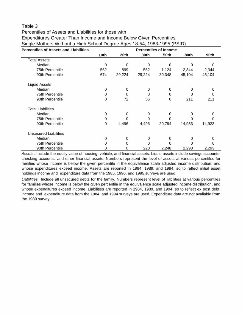
Percentiles of Assets and Liabilities Percentiles of Income10th 20th 30th 50th 80th 90th

Total AssetsMedian 0 0 0 0 0 075th Percentile 562 899 562 1,124 2,344 2,34490th Percentile 674 29,224 29,224 30,348 45,104 45,104

Liquid AssetsMedian 0 0 0 0 0 075th Percentile 0 0 0 0 0 090th Percentile 0 72 56 0 211 211

Total LiabilitiesMedian 0 0 0 0 0 075th Percentile 0 0 0 0 0 090th Percentile 0 4,496 4,496 20,794 14,933 14,933

Unsecured LiabilitiesMedian 0 0 0 0 0 075th Percentile 0 0 0 0 0 090th Percentile 0 0 220 2,248 2,293 2,293

Assets : Include the equity value of housing, vehicle, and financial assets. Liquid assets include savings accounts,checking accounts, and other financial assets. Numbers represent the level of assets at various percentiles forfamilies whose income is below the given percentile in the equivalence scale adjusted income distribution, andwhose expenditures exceed income. Assets are reported in 1984, 1989, and 1994, so to reflect initial assetholdings income and expenditure data from the 1985, 1990, and 1995 surveys are used.

Liabilities : Include all unsecured debts for the family. Numbers represent level of liabilities at various percentilesfor families whose income is below the given percentile in the equivalence scale adjusted income distribution, andwhose expenditures exceed income. Liabilities are reported in 1984, 1989, and 1994, so to reflect ex post debt,income and expenditure data from the 1984, and 1994 surveys are used. Expenditure data are not available fromthe 1989 survey.

Table 3Percentiles of Assets and Liabilities for those with Expenditures Greater Than Income and Income Below Given PercentilesSingle Mothers Without a High School Degree Ages 18-54, 1983-1995 (PSID)

Income Expenditures Ratio N(1) (2) (3) = (2)/(1) (4)

All WomenSingle mothers 20,328 23,260 1.144 6,577

(389) (379) (0.029)

Single women without children 22,683 22,569 0.995 8,390(382) (299) (0.021)

Married mothers 52,768 46,829 0.887 27,119(433) (300) (0.009)

Women Without a High School DegreeSingle mothers 12,754 15,600 1.223 1,361

(449) (416) (0.054)

Single women without children 11,344 13,224 1.166 550(639) (910) (0.104)

Married mothers 29,376 30,262 1.030 3,061(633) (521) (0.028)

Table 4Mean Income and ExpendituresSingle Mother and Comparison Households, 1991-1998 (CE)

Notes : Calculations are from the first quarter of 1992 through the first quarter of 1999 waves ofthe Consumer Expenditure Survey. Samples only includes complete income reporters. Allnumbers are indexed to 2000 dollars using the PCE deflator and are weighted. Bootstrappedstandard errors that correct for within household dependence are in parentheses.

Percentiles10th 20th 30th 50th 80th 90th

Wage = Annual Earnings/Annual Hours

All families 0.04 6.40 8.27 10.00 13.29 20.29 24.61

Single mothers without a high school degree 0.26 3.32 4.38 5.22 6.54 10.04 13.37

Reported Hourly Wage for Wage Earners OnlyAll families 0.00 7.14 8.46 9.68 12.27 17.98 20.88

Single mothers without a high school degree 0.00 5.49 6.05 6.33 7.25 9.52 11.69

Fraction Below Minimum Wage

Notes: Data come from the 1992-1999 March CPS. Samples include workers between the ages of 20 and 54 that report positive wage and salaryearnings and report working positive hours in the previous year. Workers in occupations that may not be covered by the federal minimum wageare excluded, including the following sectors: self employment, managerial and professional, sales, service, farming, forestry, fishing, and thearmed forces. Workers under the age of 20 are excluded as, in some cases, they can be exempt from the wage floor for the first 90 days ofemployment. Wages are compared to the lowest value of the federal minimum wage in the year for which the earnings are reported. All numbersare indexed to 2000 dollars using the PCE deflator and are weighted.

Table 5Wage Distribution, 1991-1999 (CPS)

Table 6Ratio of CPS March Income Supplement and SIPP Aggregate Income Estimates to

Administrative Estimates for 1996______________________________________________________________________________

Source of Income Administrative Estimate CPS (%) SIPP (%)______________________________________________________________________________Earnings 4068.3 96.1 88.4

Wages and salaries 3592.6 101.9 91.0Self-employment 475.7 52.6 69.1

Asset Income 392.6 70.9 56.6Interest 187.0 83.8 50.2Dividends 129.4 59.4 51.0Rent and Royalties 76.2 58.6 82.0

Government Transfer Income 438.3 88.3 86.3Social Security and 332.2 91.7 87.9

Railroad RetirementSupplemental Security Income 26.5 84.2 101.4Family Assistance 19.8 67.7 76.3Other Cash Welfare 3.4 80.5 114.0 Unemployment Compensation 21.6 81.6 69.4Workers’ Compensation 17.0 62.7 71.7Veterans’ Payments 17.8 89.6 72.9

Pension Income 231.9 92.6 86.1Private Pensions 98.7 93.1 98.1Federal Employee Pensions 38.8 80.8 75.6Military Retirement 28.3 58.2 101.6 State and Local Employee 66.1 57.3 67.8

Pensions

Total 5131.1 92.6 85.7______________________________________________________________________________

Source: Roemer (2000), Tables 2b, 3b, and Appendix I. The administrative estimate is an average ofthe values used to match CPS and SIPP sample coverage.

Table 7Measures of Completeness of Income Reporting in the CPS,

Various Years and Sources of Income ______________________________________________________________________________Measure of Reporting Size of Category Based Reporting Ratio

on Administrative Source(billions of current dollars)

______________________________________________________________________________

CPS AFDC/TANF benefits/Administrative AFDC/TANF payments1990 18.9 0.761997 15.9 0.63

CPS Food Stamp benefits/Administrative Food Stamp payments1990 13.6 0.761997 19.6 0.63

CPS imputed EITC payments/IRS reported EITC payments1998, All recipients 31.6 0.721998, Heads of household 21.2 0.64

______________________________________________________________________________Sources: Primus et al. (1999) Table B-4 and Meyer and Holtz-Eakin (2001) Table I.4.

Table 8Microdata Validation Evidence on Program Receipt Reporting

______________________________________________________________________________

Underreporting Share Reporting Rate Due to Failure to

Unconditional Conditional on Report IncomeTransfer Program Reporting Rate (%) True Receipt (%) Source at all (%)

(1) (2) (3)______________________________________________________________________________

AFDC 61 51 81

Food Stamps 87 77 66

SSI 88 77 84

Unemployment Insurance 80 61 63

Workers’ Compensation 82 45 NA

Social Security 101 95 NA

Veterans’ Benefits 97 83 NA______________________________________________________________________________

Notes: Column (1) reports the ratio of the number of survey individuals reporting program receipt to thenumber of survey individuals recorded as receiving program dollars in the administrative data. Column(2) reports the fraction of those who receive income from a specific program (according to theadministrative data), who report receipt in the survey data. Columns (1) and (2) are from Marquis andMoore (1990). Column (3) is the fraction of underreported months (among those underreporting atleast one month) that is attributable to a failure to report ever receiving income from the program. Column (3) is from Table 13 of Moore, Marquis, and Bogen (1996).

PCE PSID CE Ratio:

PSID/PCE Ratio:

CE/PCE (1) (2) (3) (4) = (2)/(1) (5) = (3)/(1)

Food at homea 413.9 398.3 376.2 0.96 0.91

Food away from homeb 263.9 172.8 164.9 0.65 0.62

Total food 677.8 571.1 541.1 0.84 0.80

Rentc 224.5 180.6 211.5 0.80 0.94

Table 9Comparison of PSID and CE Expenditure Measures to NationalAggregates, 1997

Source : Figures are based on the authors' calculations and are weighted to reflectthe 1997 calendar year. CE data are from the four 1997 interview surveys only.PSID figures are from the 1997 wave. We examine 1997 because the PSID addedan immigrant sample in that year. PCE aggregates come from Bureau of LaborStatistics (2001).

c CE: The sum of contract rent for the dwelling, all expenditures made by the renterfor maintenance, repair, and upkeep of the dwelling as well as decorating such aspainting and wallpaper, and tenant's insurance. PSID: Contract rent. PCE: The sumof “tenant-occupied nonfarm dwellings--rent," "rental value of farm dwellings," and"transient hotels, motels, clubs, schools, and other group housing."

b CE: The sum of food or board at school and rooming/boarding houses; cateredaffairs; food and non-alcoholic beverages at restaurants; school meals for preschooland school age children; and meals as pay. PSID: The sum of food eaten outside thehouse--excluding meals purchased while at work or while at school--and fooddelivered to the house. PCE: “Purchased meals and beverages” less “otheralcoholic beverages” with other adjustments per Bureau of Labor Statistics (2001).

a CE: The sum of food and beverages purchased and prepared on trips; food andnonalcoholic beverage purchases at grocery stores; and food and nonalcoholicbeverage purchases at convenience or specialty stores. PSID: The sum of food usedat home and the value of food stamps received. PCE: “Food purchased for off-premise consumption” less “alcoholic beverages purchased for off-premiseconsumption” less spending on pet food.

Outcome Percentiles of Income Percentiles of Consumption

0-10 10-100 Difference 0-10 10-100 DifferenceDifference in Differences

Standard Error for (7) N

(1) (2) (3) =(1) - (2) (4) (5) (6) =(4) - (5) (7) =(6) - (3) (8) (9)CE, 1991-1998

Have a stove in residence 0.962 0.971 -0.009 0.894 0.979 -0.084 -0.075 0.0427 1,361Have a microwave in residence 0.525 0.608 -0.082 0.401 0.621 -0.220 -0.138 0.0886 1,361Have a refrigerator in residence 0.969 0.976 -0.007 0.922 0.981 -0.059 -0.052 0.0374 1,361Have a freezer in residence 0.120 0.140 -0.020 0.087 0.144 -0.057 -0.037 0.0627 1,361Have a disposal in residence 0.176 0.203 -0.026 0.163 0.204 -0.041 -0.015 0.0706 1,361Have a dish washer in residence 0.122 0.138 -0.016 0.060 0.145 -0.086 -0.070 0.0531 1,361Have a clothes washer in residence 0.448 0.533 -0.084 0.367 0.542 -0.175 -0.090 0.0893 1,361Have a clothes dryer in residence 0.349 0.382 -0.032 0.189 0.399 -0.210 -0.178 0.0845 1,361Have a color television in residence 0.958 0.921 0.037 0.855 0.933 -0.077 -0.114 0.0476 1,361Have a computer in residence 0.083 0.053 0.030 0.037 0.058 -0.021 -0.052 0.0555 1,361Have a stereo in residence 0.427 0.489 -0.061 0.438 0.487 -0.049 0.012 0.0913 1,361Have a vcr in residence 0.509 0.626 -0.117 0.472 0.630 -0.158 -0.041 0.0932 1,361Have central air conditioning 0.227 0.214 0.012 0.158 0.222 -0.064 -0.076 0.0679 1,361Total # of rooms in residence (scaled) 4.065 4.135 -0.070 3.597 4.185 -0.587 -0.517 0.2326 1,361Have a car 0.416 0.464 -0.048 0.116 0.497 -0.381 -0.333 0.0779 1,361Average number of cars 0.483 0.571 -0.088 0.116 0.611 -0.495 -0.407 0.0975 1,361Took a trip or vacation 0.083 0.112 -0.029 0.020 0.119 -0.099 -0.070 0.0318 1,361Took an overnight trip or vacation 0.076 0.084 -0.008 0.014 0.091 -0.077 -0.070 0.0296 1,361Did not receive free food 0.909 0.930 -0.020 0.918 0.928 -0.010 0.011 0.0593 593

PSID, 1983-1998Total # of rooms in residence (scaled) 4.501 4.886 -0.385 4.124 4.925 -0.802 -0.417 0.2525 2,304Have some air conditioning 0.358 0.460 -0.102 0.366 0.459 -0.093 0.009 0.1134 1,501

South 0.604 0.748 -0.144 0.617 0.749 -0.132 0.013 0.1321 634Midwest/Northeast 0.160 0.262 -0.102 0.079 0.267 -0.188 -0.086 0.1095 501

Have a car 0.167 0.482 -0.316 0.361 0.461 -0.100 0.216 0.1099 1,025Average number of cars 0.200 0.584 -0.384 0.675 0.535 0.139 0.523 0.2482 660Mother does not report poor health 0.984 0.952 0.032 0.976 0.953 0.023 -0.009 0.0246 2,354Health does not limit mothers work 0.858 0.831 0.027 0.827 0.834 -0.007 -0.034 0.0600 2,260No other family members in bad health 0.984 0.955 0.029 0.919 0.962 -0.043 -0.073 0.0402 1,111Not food insecure 0.720 0.575 0.145 0.764 0.571 0.193 0.048 0.1970 158Did not go hungry 0.979 0.935 0.044 0.848 0.950 -0.102 -0.146 0.1204 158Have no children in poor health 0.995 0.984 0.011 0.994 0.984 0.011 -0.000 0.0118 743

Table 10The Relationship Between the Bottom Decile of Income or Consumption and OutcomesSingle Mothers Without a High School Degree, Ages 18-54

CE : Data are from the first quarter of 1992 through the first quarter of 1999 waves. For durables, numbers represent the fraction of the sample that either own, rent,or have access to the good in a rental unit. Income, consumption, and number of rooms are equivalence scale adjusted. Samples only include "compete incomereporters." PSID : Data are from various surveys between 1984 and 1997 depending on the availability of outcome variables. See Appendix 1 for description of how predictedconsumption is calculated in the PSID. Income, predicted consumption, and number of rooms are equivalence scale adjusted.

Outcome Percentiles of Income Percentiles of Consumption

0-10 10-100 Difference 0-10 10-100 DifferenceDifference in Differences

Standard Error for (7) N

(1) (2) (3) =(1) - (2) (4) (5) (6) =(4) - (5) (7) =(6) - (3) (8) (9)CE, 1991-1998

Have a stove in residence 0.979 0.984 -0.004 0.963 0.986 -0.023 -0.018 0.0128 6,577Have a microwave in residence 0.588 0.770 -0.182 0.480 0.782 -0.302 -0.121 0.0468 6,577Have a refrigerator in residence 0.967 0.986 -0.019 0.965 0.986 -0.022 -0.003 0.0138 6,577Have a freezer in residence 0.157 0.176 -0.019 0.120 0.181 -0.060 -0.041 0.0358 6,577Have a disposal in residence 0.238 0.334 -0.096 0.176 0.341 -0.166 -0.069 0.0348 6,577Have a dish washer in residence 0.216 0.369 -0.153 0.134 0.378 -0.243 -0.091 0.0393 6,577Have a clothes washer in residence 0.496 0.656 -0.160 0.365 0.671 -0.306 -0.146 0.0445 6,577Have a clothes dryer in residence 0.357 0.576 -0.219 0.219 0.592 -0.373 -0.154 0.0426 6,577Have a color television in residence 0.936 0.962 -0.025 0.913 0.964 -0.051 -0.026 0.0213 6,577Have a computer in residence 0.126 0.196 -0.070 0.042 0.205 -0.163 -0.093 0.0271 6,577Have a stereo in residence 0.516 0.617 -0.101 0.416 0.628 -0.212 -0.111 0.0482 6,577Have a vcr in residence 0.591 0.753 -0.162 0.507 0.763 -0.256 -0.093 0.0493 6,577Have central air conditioning 0.289 0.390 -0.100 0.241 0.395 -0.154 -0.054 0.0427 6,577Total # of rooms in residence (scaled) 4.240 5.009 -0.769 3.967 5.039 -1.071 -0.302 0.1136 6,577Have a car 0.431 0.714 -0.284 0.224 0.737 -0.514 -0.230 0.0390 6,577Average number of cars 0.522 0.980 -0.458 0.236 1.011 -0.776 -0.318 0.0541 6,577Took a trip or vacation 0.120 0.242 -0.121 0.048 0.250 -0.202 -0.081 0.0228 6,577Took an overnight trip or vacation 0.103 0.207 -0.104 0.032 0.215 -0.183 -0.079 0.0196 6,577Did not receive free food 0.939 0.961 -0.022 0.926 0.962 -0.035 -0.013 0.0285 3,046

PSID, 1983-1998Total # of rooms in residence (scaled) 4.363 5.297 -0.934 4.139 5.316 -1.177 -0.244 0.1585 7,593Have some air conditioning 0.469 0.591 -0.122 0.456 0.592 -0.137 -0.015 0.0708 5,420

South 0.616 0.858 -0.242 0.671 0.852 -0.181 0.061 0.0882 2,359Midwest/Northeast 0.326 0.457 -0.131 0.231 0.465 -0.234 -0.103 0.0901 1,658

Have a car 0.301 0.676 -0.375 0.427 0.662 -0.235 0.140 0.0700 3,032Average number of cars 0.341 0.800 -0.459 0.553 0.779 -0.227 0.232 0.1302 1,758Mother does not report poor health 0.975 0.974 0.000 0.973 0.975 -0.001 -0.002 0.0135 7,768Health does not limit mothers work 0.873 0.879 -0.006 0.853 0.881 -0.027 -0.022 0.0337 7,325No other family members in bad health 0.965 0.957 0.007 0.956 0.958 -0.003 -0.010 0.0193 3,767Not food insecure 0.669 0.778 -0.109 0.579 0.787 -0.208 -0.099 0.1120 755Did not go hungry 0.984 0.951 0.033 0.932 0.957 -0.025 -0.058 0.0428 755Have no children in poor health 0.991 0.985 0.006 0.970 0.988 -0.018 -0.024 0.0152 3,058

Table 11The Relationship Between the Bottom Decile of Income or Consumption and OutcomesAll Single Mothers, Ages 18-54

Notes : See Table 10.

Consumption Expenditures

Actual PredictedPredicted Plus

Residual Ratio Ratio Actual PredictedPredicted Plus

Residual Ratio Ratio(1) (2) (3) (4) = (2)/(1) (5) = (3)/(1) (6) (7) (8) (9) = (7)/(6) (10) = (8)/(6)

95% 31,617 28,385 29,887 0.898 0.945 32,116 30,431 30,262 0.948 0.94290% 24,677 23,885 24,774 0.968 1.004 25,747 23,470 26,264 0.912 1.02075% 18,207 17,725 17,667 0.974 0.970 18,576 18,872 18,314 1.016 0.98650% 12,753 12,740 12,595 0.999 0.988 12,685 13,527 13,203 1.066 1.04125% 9,223 10,032 9,048 1.088 0.981 9,194 10,544 9,591 1.147 1.04310% 6,748 8,034 6,777 1.190 1.004 6,681 8,743 7,357 1.309 1.1015% 5,834 7,282 5,563 1.248 0.954 5,846 7,573 6,100 1.296 1.044

Table A1Distribution of Actual and Predicted Consumption and Expenditures in the CESingle Mothers without a High School Degree, 1991-1998

Notes : Calculations are from the first quarter of 1992 through the first quarter of 1999 waves of the Consumer Expenditure Survey. All numbers are indexed to 2000 dollars using the PCE deflator and are weighted.