Embed Size (px)
Citation preview

NATIONAL CENTER FOR EDUCATION STATISTICS
Statistical Analysis Report March 2001
Postsecondary Education Descriptive Analysis Reports
Attrition of New Teachers AmongRecent College GraduatesComparing Occupational Stability Among 1992–93Graduates Who Taught and Those Who Worked in OtherOccupations
Robin R. HenkeLisa ZahnMPR Associates, Inc.
C. Dennis CarrollNational Center for Education Statistics
U.S. Department of EducationOffice of Educational Research and Improvement NCES 2001–189
U.S. Department of EducationRod PaigeSecretary
National Center for Education StatisticsGary W. PhillipsActing Commissioner
The National Center for Education Statistics (NCES) is the primary federal entity for collecting, analyzing, andreporting data related to education in the United States and other nations. It fulfills a congressional mandate tocollect, collate, analyze, and report full and complete statistics on the condition of education in the United States;conduct and publish reports and specialized analyses of the meaning and significance of such statistics; assist stateand local education agencies in improving their statistical systems; and review and report on education activities inforeign countries.
NCES activities are designed to address high priority education data needs; provide consistent, reliable, complete,and accurate indicators of education status and trends; and report timely, useful, and high quality data to the U.S.Department of Education, the Congress, the states, other education policymakers, practitioners, data users, and thegeneral public.
We strive to make our products available in a variety of formats and in language that is appropriate to a variety ofaudiences. You, as our customer, are the best judge of our success in communicating information effectively. If youhave any comments or suggestions about this or any other NCES product or report, we would like to hear from you.Please direct your comments to:
National Center for Education StatisticsOffice of Educational Research and ImprovementU.S. Department of Education1990 K Street NWWashington, DC 20006-5574
March 2001
The NCES World Wide Web Home Page is: http://nces.ed.govThe NCES World Wide Web Electronic Catalog is: http://nces.ed.gov/pubsearch/index.asp
Suggested CitationU.S. Department of Education. National Center for Education Statistics. Attrition of New Teachers AmongRecent College Graduates: Comparing Occupational Stability Among 1992–93 Graduates Who Taughtand Those Who Worked in Other Occupations, NCES 2001–189, by Robin R. Henke and Lisa Zahn.Project Officer: C. Dennis Carroll. Washington, DC: 2001.
For ordering information on this report, write:U.S. Department of EducationED PubsP.O. Box 1398Jessup, MD 20794-1398
or call toll free 1-877-4ED-PUBS or go to the Internet: http://www.ed.gov/pubs/edpubs.html
Contact:Aurora D’Amico(202) 502-7334

iii
Executive Summary
News reports frequently discuss the shortage ofelementary/secondary teachers in the UnitedStates. Increasing enrollments, particularly in theelementary grades; increasing rates of retirementamong teachers; and the efforts of states and lo-calities to reduce class size may well have contrib-uted to many of these shortages (Johnson 2001). Inrecent years, enrollments in public and privateelementary and secondary schools have grownconsiderably, and most expect that they will con-tinue to climb through 2005, after which they areexpected to drop slightly through 2010 (Geraldand Hussar 2000). Nevertheless, shortages maywell continue since the proportion of teachers whoretire each year is expected to rise (Goodnough2000). As experienced baby-boomer teachers re-tire, they are likely to be replaced by young andinexperienced teachers, whose attrition rates arehigher than those of mid-career teachers (Archer1999; Grissmer and Kirby 1997).1
Many researchers and policymakers attributethe higher attrition rate among new teachers totheir working conditions (e.g., Baker and Smith1997). Therefore, to encourage new teachers toremain in the profession, many states and localitieshave launched programs to support them (Archer1999; Cooperman 2000). Policy analysts have also
1Schools and Staffing Survey (SASS) data from 1994–95indicate that about 8 percent of teachers who had taught lessthan 4 years left the profession since the previous school year,and that about 7 percent of teachers with 4 to 9 years of expe-rience did so (Whitener et al. 1997). In contrast, between 4and 5 percent of teachers with 10 to 24 years of experienceleft between 1993–94 and 1994–95. Other SASS estimatesindicate that approximately 30 percent of new teachers leavethe profession within the first 5 years of entry (Ingersoll ascited in Archer 1999).
recommended that schools and districts profes-sionalize teaching to improve retention (Kansto-room and Finn 1999; Holmes Group 1986;National Commission on Teaching and America’sFuture (NCTAF) 1996, 1997).
Such policy initiatives may help new teachersbecome better teachers more quickly and may in-crease occupation stability among all teachers;however, they do not address other possible rea-sons for attrition among new teachers. Althoughsuch attrition has received considerable researchattention over the years (Darling-Hammond 1984;Murnane et al. 1991), whether new teachers aremore likely than college graduates beginning ca-reers in other professions to change occupationshas not yet been addressed. High attrition frominitial occupations may be endemic to new collegegraduates’ entry into the labor market, regardlessof occupation, as new graduates learn about theworkplace and about their strengths and weak-nesses as well as what they like and dislike abouttheir jobs. In addition, interest or aptitude for afield in an academic setting may not always trans-late into satisfaction in a related occupation. Par-ticularly among graduates who majored inacademic, rather than applied, fields of study, in-formation about the kinds of work available tothem and their affinity for it may be limited. Ifnew college graduates change occupations atsimilar rates regardless of their early occupations,reducing attrition among new teachers may be asmuch a matter of helping college students and newgraduates choose, plan, and prepare for their ca-reers as supporting new teachers and profession-alizing teaching.

Executive Summary
iv
This research examines the occupation stabilityof bachelor’s degree recipients during the first 4years after receiving the bachelor’s degree. Theanalyses address the following question: weregraduates who were teaching in 1994 more or lesslikely than those in other occupations to leave thework force or work in a different occupation in1997?
Data and Methodology
The 1993 Baccalaureate and Beyond Longitu-dinal Study (B&B:93) provided the data for theseanalyses. NCES first surveyed a nationally repre-sentative sample of about 11,200 students whoreceived bachelor’s degrees between July 1, 1992and June 30, 1993 in the spring of 1993, and thenagain in 1994 and 1997. These analyses are basedon the 83 percent of the original sample, about9,300 graduates, who participated in all three B&Bsurvey administrations.
The B&B data provide an important opportu-nity to compare the behavior of a significant pro-portion of new teachers to that of theirnonteaching peers. However, results from theseanalyses cannot be generalized to all new teachersin 1994 or 1997 because many new teachers donot begin teaching immediately after completing abachelor’s degree.
These analyses are based largely on compositevariables developed from graduates’ reports ofwhat they were doing during both April 1994 and1997. Composites were created to summarizegraduates’ major activities (e.g., working, study-ing, or both) in 1994 and 1997, whether their ma-jor activities differed between April 1994 andApril 1997, and whether their occupations differedbetween the two years.
Results
Teaching and Teacher Attrition Among1992–93 Bachelor’s Degree Recipients
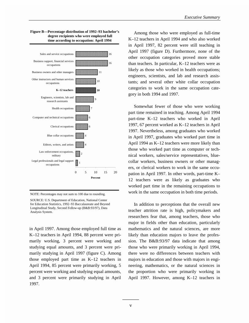
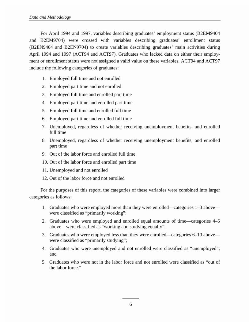
In April 1994, 80 percent of 1992–93 graduateswere primarily working,2 and another 3 percentcombined study and work equally. The remaininggraduates were primarily studying (11 percent),were not enrolled and either unemployed (3 per-cent) or were out of the labor force (3 percent)(figure A). Kindergarten through 12th-gradeteachers made up 10 percent of graduates whowere working full time in April 1994 (figure B).
Figure A—Percentage distribution of 1992–93 bachelor’sFigure A—degree recipients according to main activity: Figure A—April 1994
NOTE: Percentages may not sum to 100 due to rounding.
SOURCE: U.S. Department of Education, National Center for Education Statistics, 1992–93 Baccalaureate and BeyondLongitudinal Study, Second Follow-up (B&B:93/97),Data Analysis System.
80
3
113 3
Primarily working Working and studying equally Primarily studying Not enrolled, unemployed Not enrolled, out of the labor force
Whether they were employed full time or parttime in April 1994, most graduates who worked asK–12 teachers in April 1994 were also employed
2Graduates who were primarily working were working forpay full time or part time, but they were working more thanthey were studying. This category includes graduates whowere working full time and either not enrolled or enrolled parttime and graduates who were working part time and not en-rolled.
Executive Summary
v
Figure B—Percentage distribution of 1992–93 bachelor’sFigure A—degree recipients who were employed full Figure A—time according to occupation: April 1994
NOTE: Percentages may not sum to 100 due to rounding.
SOURCE: U.S. Department of Education, National Center for Education Statistics, 1992–93 Baccalaureate and BeyondLongitudinal Study, Second Follow-up (B&B:93/97), Data Analysis System.
1
2
4
6
7
9
10
11
16
16
4
10
6
0 5 10 15 20
Legal professionals and legal supportoccupations
Law enforcement occupations,military
Editors, writers, and artists
Blue collar occupations
Clerical occupations
Computer and technical occupations
Health occupations
Engineers, scientists, lab andresearch assistants
K–12 teachers
Other instructors and human servicesoccupations
Business owners and other managers
Business support, financial servicesoccupations
Sales and service occupations
Percent
K–12 teachers
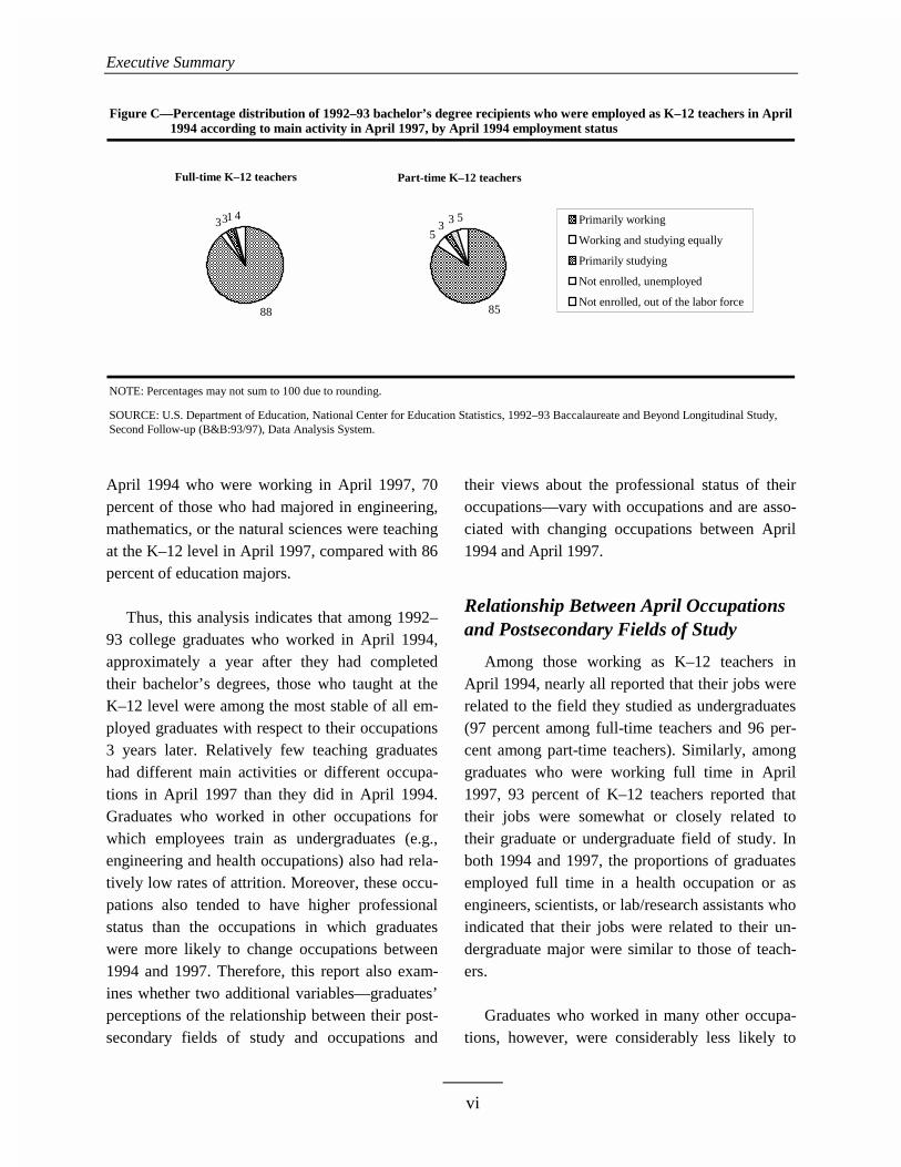
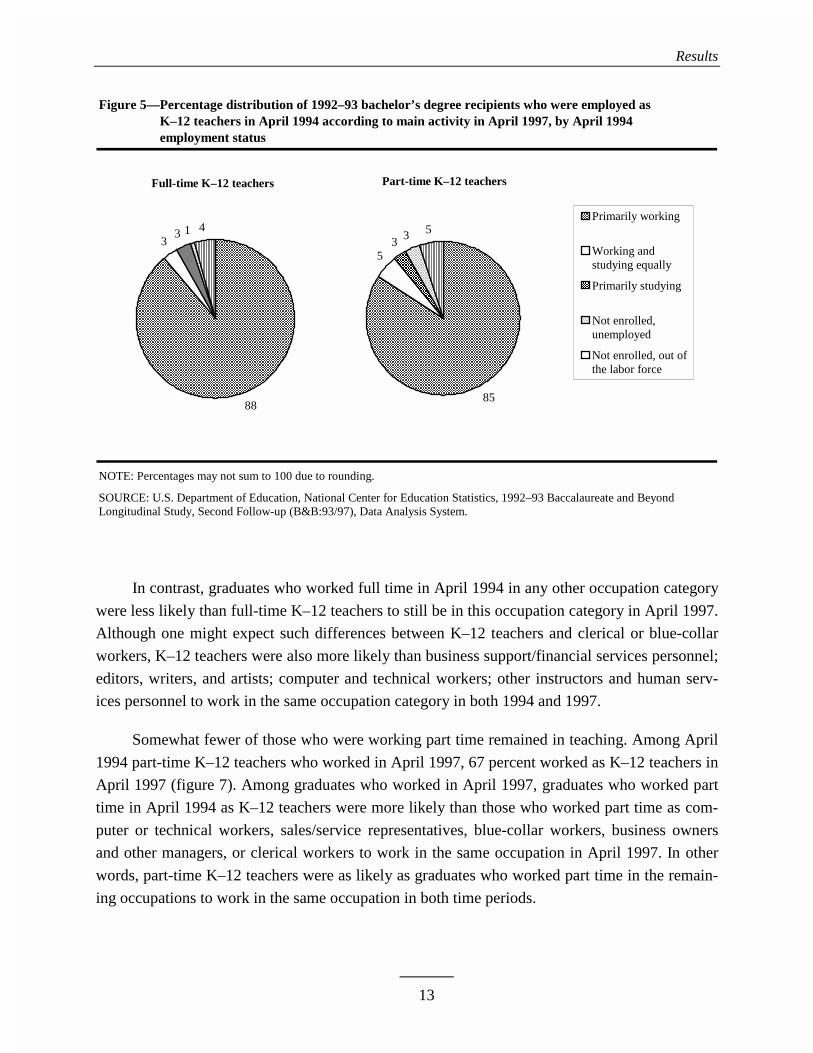
in April 1997. Among those employed full time asK–12 teachers in April 1994, 88 percent were pri-marily working, 3 percent were working andstudying equal amounts, and 3 percent were pri-marily studying in April 1997 (figure C). Amongthose employed part time as K–12 teachers inApril 1994, 85 percent were primarily working, 5percent were working and studying equal amounts,and 3 percent were primarily studying in April1997.
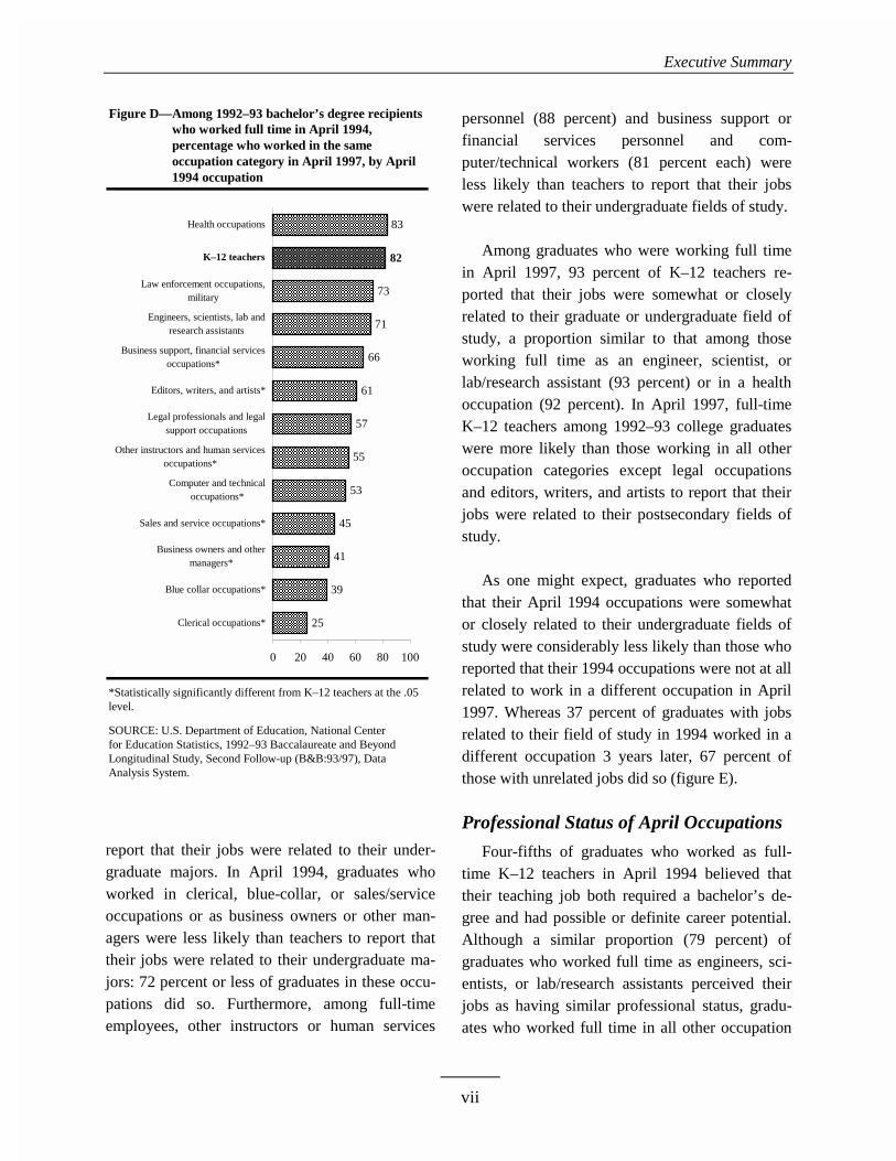
Among those who were employed as full-timeK–12 teachers in April 1994 and who also workedin April 1997, 82 percent were still teaching inApril 1997 (figure D). Furthermore, none of theother occupation categories proved more stablethan teachers. In particular, K–12 teachers were aslikely as those who worked in health occupations;engineers, scientists, and lab and research assis-tants; and several other white collar occupationcategories to work in the same occupation cate-gory in both 1994 and 1997.
Somewhat fewer of those who were workingpart time remained in teaching. Among April 1994part-time K–12 teachers who worked in April1997, 67 percent worked as K–12 teachers in April1997. Nevertheless, among graduates who workedin April 1997, graduates who worked part time inApril 1994 as K–12 teachers were more likely thanthose who worked part time as computer or tech-nical workers, sales/service representatives, blue-collar workers, business owners or other manag-ers, or clerical workers to work in the same occu-pation in April 1997. In other words, part-time K–12 teachers were as likely as graduates whoworked part time in the remaining occupations towork in the same occupation in both time periods.
In addition to perceptions that the overall newteacher attrition rate is high, policymakers andresearchers fear that, among teachers, those whomajor in fields other than education, particularlymathematics and the natural sciences, are morelikely than education majors to leave the profes-sion. The B&B:93/97 data indicate that amongthose who were primarily working in April 1994,there were no differences between teachers withmajors in education and those with majors in engi-neering, mathematics, or the natural sciences inthe proportion who were primarily working inApril 1997. However, among K–12 teachers in
Executive Summary
vi
Figure C—Percentage distribution of 1992–93 bachelor’s degree recipients who were employed as K–12 teachers in April Figure 5—1994 according to main activity in April 1997, by April 1994 employment status
NOTE: Percentages may not sum to 100 due to rounding.
SOURCE: U.S. Department of Education, National Center for Education Statistics, 1992–93 Baccalaureate and Beyond Longitudinal Study,Second Follow-up (B&B:93/97), Data Analysis System.
Full-time K–12 teachers
88
331 4
Part-time K–12 teachers
85
5
53 3 Primarily working
Working and studying equally
Primarily studying
Not enrolled, unemployed
Not enrolled, out of the labor force
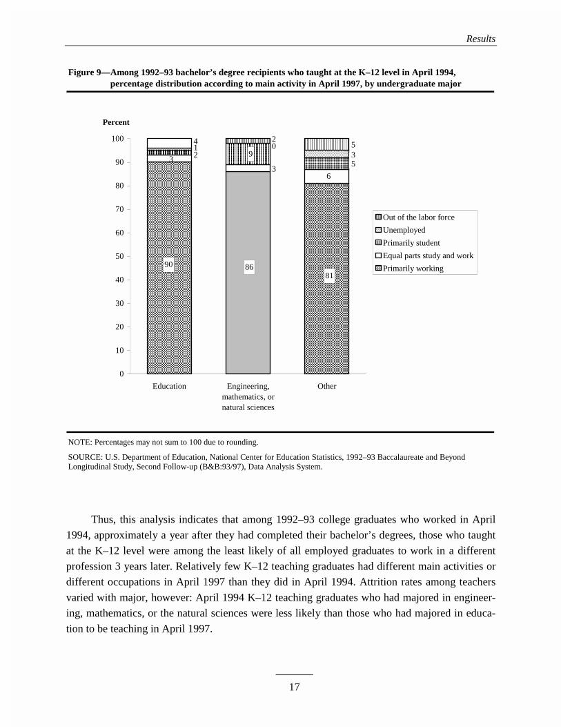
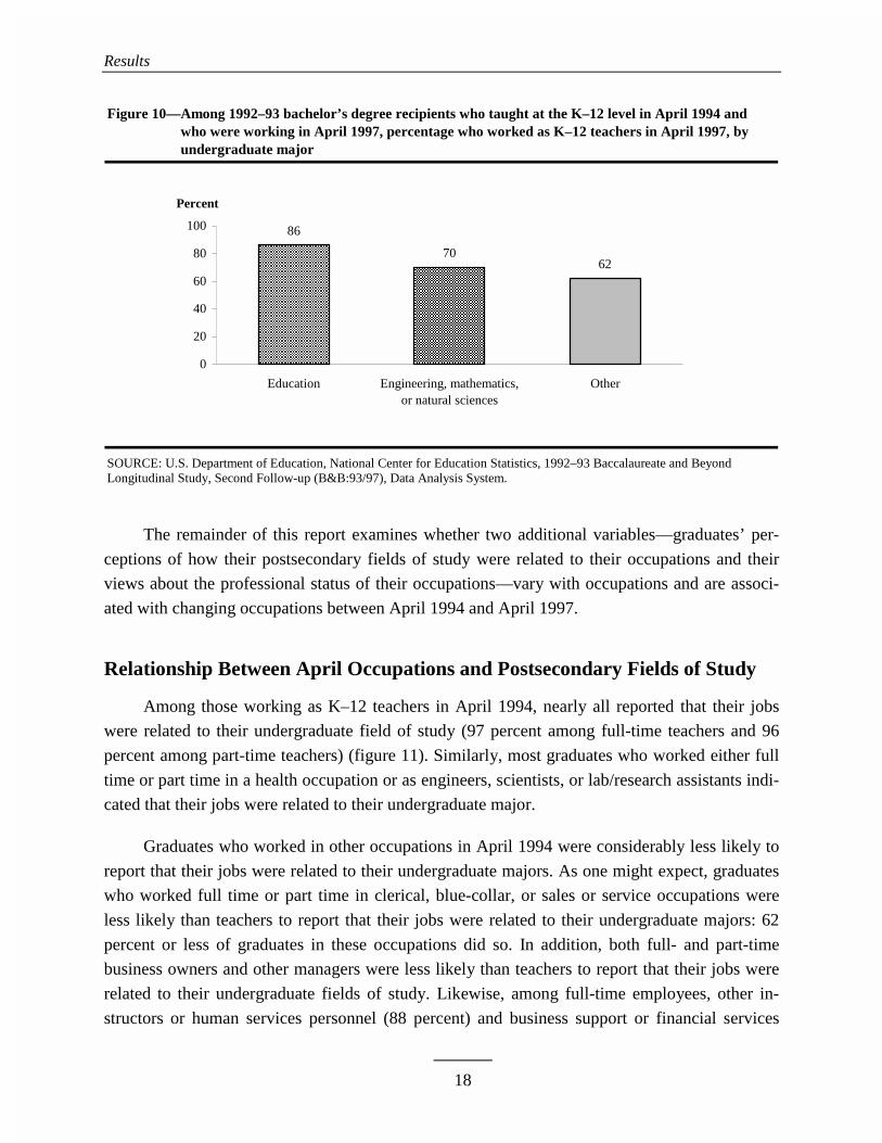
April 1994 who were working in April 1997, 70percent of those who had majored in engineering,mathematics, or the natural sciences were teachingat the K–12 level in April 1997, compared with 86percent of education majors.
Thus, this analysis indicates that among 1992–93 college graduates who worked in April 1994,approximately a year after they had completedtheir bachelor’s degrees, those who taught at theK–12 level were among the most stable of all em-ployed graduates with respect to their occupations3 years later. Relatively few teaching graduateshad different main activities or different occupa-tions in April 1997 than they did in April 1994.Graduates who worked in other occupations forwhich employees train as undergraduates (e.g.,engineering and health occupations) also had rela-tively low rates of attrition. Moreover, these occu-pations also tended to have higher professionalstatus than the occupations in which graduateswere more likely to change occupations between1994 and 1997. Therefore, this report also exam-ines whether two additional variables—graduates’perceptions of the relationship between their post-secondary fields of study and occupations and
their views about the professional status of theiroccupations—vary with occupations and are asso-ciated with changing occupations between April1994 and April 1997.
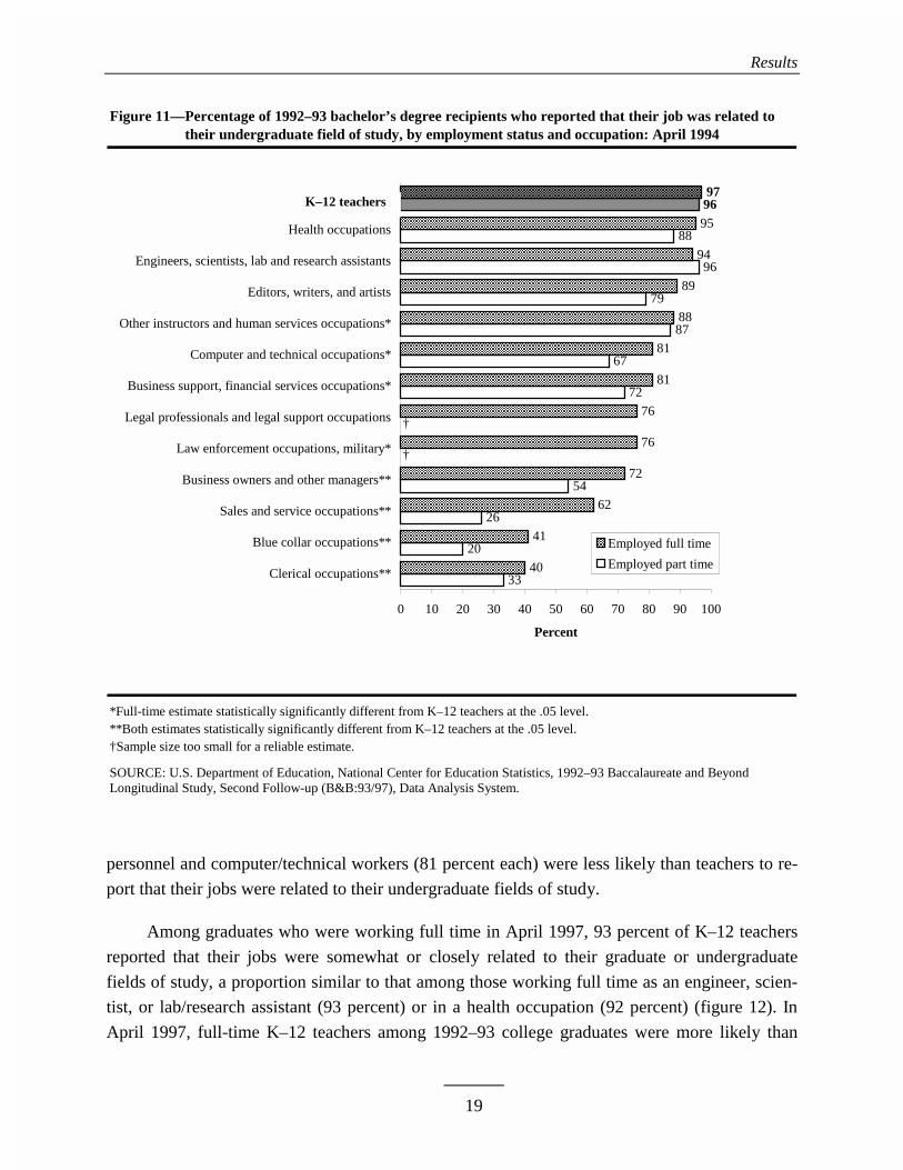
Relationship Between April Occupationsand Postsecondary Fields of Study
Among those working as K–12 teachers inApril 1994, nearly all reported that their jobs wererelated to the field they studied as undergraduates(97 percent among full-time teachers and 96 per-cent among part-time teachers). Similarly, amonggraduates who were working full time in April1997, 93 percent of K–12 teachers reported thattheir jobs were somewhat or closely related totheir graduate or undergraduate field of study. Inboth 1994 and 1997, the proportions of graduatesemployed full time in a health occupation or asengineers, scientists, or lab/research assistants whoindicated that their jobs were related to their un-dergraduate major were similar to those of teach-ers.
Graduates who worked in many other occupa-tions, however, were considerably less likely to
Executive Summary
vii
Figure D—Among 1992–93 bachelor’s degree recipients Figure A—who worked full time in April 1994, Figure A—percentage who worked in the same Figure A—occupation category in April 1997, by April Figure A—1994 occupation
*Statistically significantly different from K–12 teachers at the .05level.
SOURCE: U.S. Department of Education, National Center for Education Statistics, 1992–93 Baccalaureate and BeyondLongitudinal Study, Second Follow-up (B&B:93/97), DataAnalysis System.
K–12
25
39
41
45
53
55
57
61
66
71
73
83
82
0 20 40 60 80 100
Clerical occupations*
Blue collar occupations*
Business owners and othermanagers*
Sales and service occupations*
Computer and technicaloccupations*
Other instructors and human servicesoccupations*
Legal professionals and legalsupport occupations
Editors, writers, and artists*
Business support, financial servicesoccupations*
Engineers, scientists, lab andresearch assistants
Law enforcement occupations,military
K–12 teachers
Health occupations
K–12 teachers
report that their jobs were related to their under-graduate majors. In April 1994, graduates whoworked in clerical, blue-collar, or sales/serviceoccupations or as business owners or other man-agers were less likely than teachers to report thattheir jobs were related to their undergraduate ma-jors: 72 percent or less of graduates in these occu-pations did so. Furthermore, among full-timeemployees, other instructors or human services
personnel (88 percent) and business support orfinancial services personnel and com-puter/technical workers (81 percent each) wereless likely than teachers to report that their jobswere related to their undergraduate fields of study.
Among graduates who were working full timein April 1997, 93 percent of K–12 teachers re-ported that their jobs were somewhat or closelyrelated to their graduate or undergraduate field ofstudy, a proportion similar to that among thoseworking full time as an engineer, scientist, orlab/research assistant (93 percent) or in a healthoccupation (92 percent). In April 1997, full-timeK–12 teachers among 1992–93 college graduateswere more likely than those working in all otheroccupation categories except legal occupationsand editors, writers, and artists to report that theirjobs were related to their postsecondary fields ofstudy.
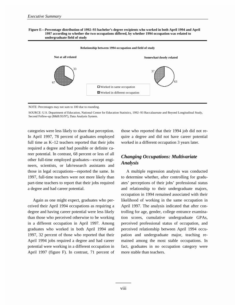
As one might expect, graduates who reportedthat their April 1994 occupations were somewhator closely related to their undergraduate fields ofstudy were considerably less likely than those whoreported that their 1994 occupations were not at allrelated to work in a different occupation in April1997. Whereas 37 percent of graduates with jobsrelated to their field of study in 1994 worked in adifferent occupation 3 years later, 67 percent ofthose with unrelated jobs did so (figure E).
Professional Status of April Occupations
Four-fifths of graduates who worked as full-time K–12 teachers in April 1994 believed thattheir teaching job both required a bachelor’s de-gree and had possible or definite career potential.Although a similar proportion (79 percent) ofgraduates who worked full time as engineers, sci-entists, or lab/research assistants perceived theirjobs as having similar professional status, gradu-ates who worked full time in all other occupation
Executive Summary
viii
Figure E—Percentage distribution of 1992–93 bachelor’s degree recipients who worked in both April 1994 and April Figure E—1997 according to whether the two occupations differed, by whether 1994 occupation was related to Figure E—undergraduate field of study
NOTE: Percentages may not sum to 100 due to rounding.
SOURCE: U.S. Department of Education, National Center for Education Statistics, 1992–93 Baccalaureate and Beyond Longitudinal Study, Second Follow-up (B&B:93/97), Data Analysis System.
Relationship between 1994 occupation and field of study
Not at all related
33
67
Somewhat/closely related
63
37
Worked in same occupation
Worked in different occupation
categories were less likely to share that perception.In April 1997, 78 percent of graduates employedfull time as K–12 teachers reported that their jobsrequired a degree and had possible or definite ca-reer potential. In contrast, 68 percent or less of allother full-time employed graduates—except engi-neers, scientists, or lab/research assistants andthose in legal occupations—reported the same. In1997, full-time teachers were not more likely thanpart-time teachers to report that their jobs requireda degree and had career potential.
Again as one might expect, graduates who per-ceived their April 1994 occupations as requiring adegree and having career potential were less likelythan those who perceived otherwise to be workingin a different occupation in April 1997. Amonggraduates who worked in both April 1994 and1997, 32 percent of those who reported that theirApril 1994 jobs required a degree and had careerpotential were working in a different occupation inApril 1997 (figure F). In contrast, 71 percent of
those who reported that their 1994 job did not re-quire a degree and did not have career potentialworked in a different occupation 3 years later.
Changing Occupations: MultivariateAnalysis
A multiple regression analysis was conductedto determine whether, after controlling for gradu-ates’ perceptions of their jobs’ professional statusand relationship to their undergraduate majors,occupation in 1994 remained associated with theirlikelihood of working in the same occupation inApril 1997. The analysis indicated that after con-trolling for age, gender, college entrance examina-tion scores, cumulative undergraduate GPAs,perceived professional status of occupation, andperceived relationship between April 1994 occu-pation and undergraduate major, teaching re-mained among the most stable occupations. Infact, graduates in no occupation category weremore stable than teachers.

Executive Summary
ix
Figure F—Percentage distribution of 1992–93 bachelor’s degree recipients who worked in both April 1994 and April Figure F—1997 according to whether the two occupations differed, by whether 1994 occupation required a bachelor’s Figure F—degree and had career potential
NOTE: Percentages may not sum to 100 due to rounding.
SOURCE: U.S. Department of Education, National Center for Education Statistics, 1992–93 Baccalaureate and Beyond Longitudinal Study,Second Follow-up (B&B:93/97), Data Analysis System.
No degree required/possible or definite potential
4852
No degree required/not much potential
29
71
Degree required/possible or definite potential
68
32
Degree required/not much potential
58
42
Worked in same occupation
Worked in different occupation
Degree required/possible or definite potential
Graduates’ perceptions of their April 1994job’s professional status and of the relationshipbetween their undergraduate field of study andtheir April 1994 job were, independently, relatedto whether they worked in the same occupationcategory at both points in time. Graduates whoperceived their April 1994 job as unrelated orsomewhat related to their undergraduate majorfield of study were less likely than those who per-ceived a close relationship to work in the sameoccupation in 1997 as in 1994. Graduates who re-ported that a degree was required to obtain theirApril 1994 occupation were more likely to work inthe same occupation category at both points in
time than were graduates who did not, althoughgraduates’ perceptions of the career potential oftheir jobs appeared not to make a difference.
Summary
Among graduates who were employed in April1994 and April 1997, K–12 teachers (i.e., gradu-ates who taught in 1994) were as likely as gradu-ates who worked in other white collar,professional occupations to work in the same oc-cupation category in April 1997. Specifically, ap-proximately four-fifths of graduates who taught inApril 1994 were also teaching in April 1997, and

Executive Summary
x
similar proportions of graduates who worked inhealth occupations; as engineers, scientists,lab/research assistants; in legal occupations; in lawenforcement or the military; or as business sup-port/financial services workers worked in their
respective occupation categories in both April1994 and April 1997. Graduates who worked inother occupation categories in April 1994 wereless likely than K–12 teachers to work in the sameoccupation category at both points in time.

xi
Foreword
Although elementary/secondary school teachers are frequently the object of research atten-
tion, few data sources allow researchers to examine the career paths of teachers in the context of
similarly educated employees in other occupations. Therefore, although education researchers
have developed a considerable body of research on teachers’ careers, it has not been clear
whether or how teachers’ careers differ from the career paths of other college graduates.
The 1993 Baccalaureate and Beyond Longitudinal Study (B&B:93) provides a unique op-
portunity to study such questions. B&B:93 has surveyed a sample of 1992–93 college graduates
three times: in 1993, 1994, and 1997. These data allow researchers to study relationships be-
tween graduates’ undergraduate experiences and their subsequent choices and experiences in
graduate education and employment. In particular, each of the three surveys has included a com-
ponent related to elementary/secondary teaching. This report takes advantage of these data to
compare the later occupation choices made by graduates who taught early in their postbaccalau-
reate careers with those made by graduates who worked in other fields in the year following col-
lege graduation.
xii
Acknowledgments
The authors are grateful to staff members at MPR Associates, NCES and other U.S. De-
partment of Education offices, and nongovernmental agencies for their contributions to the pro-
duction of this report. At MPR Associates, the work of Sonya Geis in the recoding process that
yielded variables used in the report was invaluable. Chloe Huynh assisted with estimate genera-
tion and statistical testing. Laura Horn and the entire postsecondary group provided helpful
comments on preliminary findings and earlier drafts. Members of the production team—Fran-
cesca Tussing, Andrea Livingston, Renee Macalino, and Barbara Kridl—took care of the word
processing, editing, proofreading, and overall production management, respectively.
Outside of MPR Associates, C. Dennis Carroll, Paula Knepper, Rosalind Korb, Stephen
Broughman, and John Ralph at NCES reviewed the report at various stages and provided very
useful feedback. Elsewhere in the U.S. Department of Education, Karen Wenk of the Office of
Postsecondary Education, Alexander Choi of the Office for Civil Rights, and Edith Harvey of the
Office of Elementary and Secondary Education also reviewed the report and commented on it.
Finally, Brian Trzebiatowski from the Association of State Colleges and Universities provided
clarifying comments.
xiii
Table of Contents
PageExecutive Summary .................................................................................................................. iiiForeword .................................................................................................................................... xiAcknowledgments...................................................................................................................... xiiList of Tables ............................................................................................................................. xivList of Figures ............................................................................................................................ xv
Introduction ............................................................................................................................... 1
Data and Methodology.............................................................................................................. 5
Results ........................................................................................................................................ 9Relationship Between April Occupations and Postsecondary Fields of Study..................... 18Professional Status of April Occupations.............................................................................. 21Changing Occupations: Multivariate Analysis ..................................................................... 24
Conclusion.................................................................................................................................. 29
References .................................................................................................................................. 33
Appendix A—Glossary ............................................................................................................. 35
Appendix B—Technical Notes and Methodology .................................................................. 43

xiv
List of Tables
Table Page
1 Among 1992–93 bachelor’s degree recipients who were employed in both April 1994and April 1997 percentage who worked in the same occupation category at the twopoints in time, unadjusted and adjusted after controlling for variables listed in thetable ................................................................................................................................ 26
Appendix Tables
B1a Standard errors for Figures 2 and 4: Percentage distribution of employed 1992–93bachelor’s degree recipients according to occupation, by employment status: April1994................................................................................................................................. 45
B1b Standard errors for Figures 2 and 4: Percentage distribution of employed 1992–93bachelor’s degree recipients according to occupation, by employment status: April1994................................................................................................................................. 45

xv
List of Figures
Figure Page
A Percentage distribution of 1992–93 bachelor’s degree recipients according to mainactivity: April 1994 ......................................................................................................... iv
B Percentage distribution of 1992–93 bachelor’s degree recipients who were employedfull time according to occupation: April 1994 ................................................................ v
C Percentage distribution of 1992–93 bachelor’s degree recipients who were employedas K–12 teachers in April 1994 according to main activity in April 1997, by April1994 employment status.................................................................................................. vi
D Among 1992–93 bachelor’s degree recipients who worked full time in April 1994,percentage who worked in the same occupation category in April 1997, by April 1994occupation ....................................................................................................................... vii
E Percentage distribution of 1992–93 bachelor’s degree recipients who worked in bothApril 1994 and April 1997 according to whether the two occupations differed, bywhether 1994 occupation was related to undergraduate field of study........................... viii
F Percentage distribution of 1992–93 bachelor’s degree recipients who worked in bothApril 1994 and April 1997 according to whether the two occupations differed, bywhether 1994 occupation required a bachelor’s degree and had career potential........... ix
1 Percentage distribution of 1992–93 bachelor’s degree recipients according to mainactivity: April 1994 ......................................................................................................... 9
2 Percentage distribution of 1992–93 bachelor’s degree recipients who were employedfull time according to occupation: April 1994 ................................................................ 10
3 Percentage of 1992–93 bachelor’s degree recipients who were employed full time, byoccupation: April 1994.................................................................................................... 11
4 Percentage distribution of 1992–93 bachelor’s degree recipients who were employedpart time according to occupation: April 1994................................................................ 12
5 Percentage distribution of 1992–93 bachelor’s degree recipients who were employedas K–12 teachers in April 1994 according to main activity in April 1997, by April1994 employment status.................................................................................................. 13

List of Figures
xvi
Figure Page
6 Among 1992–93 bachelor’s degree recipients who worked full time in April 1994,percentage who worked in the same occupation category in April 1997, by April 1994occupation ....................................................................................................................... 14
7 Among 1992–93 bachelor’s degree recipients who worked part time in April 1994,percentage who worked in the same occupation category in April 1997, by April 1994occupation ....................................................................................................................... 15
8 Among 1992–93 bachelor’s degree recipients who were primarily working andemployed full time in April 1994, percentages who had enrolled at the postsecondaryand at the graduate levels by April 1997, by April 1994 occupation.............................. 16
9 Among 1992–93 bachelor’s degree recipients who taught at the K–12 level in April1994, percentage distribution according to main activity in April 1997, byundergraduate major........................................................................................................ 17
10 Among 1992–93 bachelor’s degree recipients who taught at the K–12 level in April1994 and who were working in April 1997, percentage who worked as K–12 teachersin April 1997, by undergraduate major ........................................................................... 18
11 Percentage of 1992–93 bachelor’s degree recipients who reported that their job wasrelated to their undergraduate field of study, by employment status and occupation:April 1994 ....................................................................................................................... 19
12 Percentage of 1992–93 bachelor’s degree recipients who reported that their job wasrelated to their undergraduate or graduate field of study, by employment status andoccupation: April 1997.................................................................................................... 20
13 Percentage distribution of 1992–93 bachelor’s degree recipients who worked in bothApril 1994 and April 1997 according to whether the two occupations differed, bywhether 1994 occupation was related to undergraduate field of study........................... 22
14 Percentage of 1992–93 bachelor’s degree recipients who reported that their job hadcareer potential and that a bachelor’s degree was required to obtain the job, byemployment status and occupation: April 1994.............................................................. 23
15 Percentage of 1992–93 bachelor’s degree recipients who reported that their job hadcareer potential and that a bachelor’s degree was required to obtain the job, byemployment status and occupation: April 1997.............................................................. 24
16 Percentage distribution of 1992–93 bachelor’s degree recipients who worked in bothApril 1994 and April 1997 according to whether the two occupations differed, bywhether 1994 occupation required a bachelor’s degree and had career potential........... 25
1
Introduction
Although researchers have predicted teacher shortages for more than 15 years, it appears
that as the century came to a close, these shortages had arrived.1 The teacher shortages experi-
enced in 1999–2000 were both field- and location-specific. For example, consumer sciences
teachers in particular (Zehr 1998b) and vocational education teachers in general (Zehr 1998a)
have been in short supply in many districts, and special education teachers are chronically diffi-
cult to hire (Sack 1999). In addition, particular states and localities are finding it harder than oth-
ers to staff elementary/secondary classrooms (Archibold 1999; Steinberg 1999; Wilgoren 1999),
and often these shortages occur in selected fields rather than across fields (Bradley 1999).
Increasing enrollments, particularly in the elementary grades; increasing rates of retirement
among teachers; and the efforts of states and localities to reduce class size may well have con-
tributed to many of these shortages (Johnson 2001). In recent years, enrollments in public and
private elementary and secondary schools have grown considerably, and most expect that they
will continue to climb through 2005, after which they are expected to drop slightly through 2010
(Gerald and Hussar 2000). Nevertheless, shortages may well continue since the proportion of
teachers who retire each year is expected to rise (Goodnough 2000). As experienced baby-
boomer teachers retire, they are likely to be replaced by young and inexperienced teachers,
whose attrition rates are higher than those of mid-career teachers (Archer 1999; Grissmer and
Kirby 1997).2
Many researchers and policymakers attribute the higher attrition rate among new teachers
to their working conditions (e.g., Baker and Smith 1997). New teachers generally assume the
same responsibilities that experienced teachers have and, unlike many other professions where
new professionals are supervised by a more experienced colleague, often do so without the sup-
port of a mentor or supervisor. In addition, conventional wisdom maintains that new teachers re-
ceive the most difficult assignments (Archer 1999), which is consistent with data indicating that
1Schools and Staffing Survey (SASS) data collected between 1987–88 and 1993–94 did not provide evidence of general or spe-cific teacher shortages in the U.S., despite predictions that such shortages would occur in the late 1980s and early 1990s (Darling-Hammond 1984; Henke, Choy, Geis, and Broughman 1996).2Schools and Staffing Survey (SASS) data from 1994–95 indicate that about 8 percent of teachers who had taught less than 4years left the profession since the previous school year, and that about 7 percent of teachers with 4 to 9 years of experience did so(Whitener et al. 1997). In contrast, between 4 and 5 percent of teachers with 10 to 24 years of experience left between 1993–94and 1994–95. Other SASS estimates indicate that approximately 30 percent of new teachers leave the profession within the first 5years of entry (Ingersoll as cited in Archer 1999).

Introduction
2
teachers in schools serving large proportions of poor children have less experience than teachers
serving more affluent children (Henke, Choy, Chen, Geis, and Alt 1997).
To encourage new teachers to remain in the profession, many states and localities have
launched programs to support them. New Jersey, for example, created an alternative teacher
preparation track, which provided new teachers with support from principals and experienced
teachers (Cooperman 2000). Teachers who participated in this program left teaching at a rate of
about 4 percent annually between 1984 and 1990, whereas teachers in the traditional teacher
preparation track, which did not provide such support, left at a rate of 16 percent. In California,
the Beginning Teacher Support and Assessment (BTSA) Program has grown dramatically in re-
cent years as the state attempts to improve its rate of retaining new teachers. BTSA provides new
teachers with mentors—experienced teachers who help new teachers solve problems, self-assess
their weaknesses, and improve their teaching skills in the first 2 years of teaching. Some local
BTSA programs are reporting retention rates of 85 to 90 percent (Archer 1999).
Policy analysts have also recommended that schools and districts professionalize teaching
to improve retention (Kanstoroom and Finn 1999; Holmes Group 1986; National Commission on
Teaching and America’s Future (NCTAF) 1996, 1997). Specific measures to professionalize
teaching include giving teachers more responsibility for school governance, creating career lad-
ders for teachers, and increasing teacher salaries—particularly among experienced teachers—ei-
ther across the board or according to merit. Since educators and analysts have noted that teachers
with better preservice preparation are more likely than others to remain in the profession, many
have proposed improving teacher preparation as a way to reduce teacher attrition and improve
the quality of instruction.
Such policy initiatives may help new teachers become better teachers more quickly and
may increase occupation stability among all teachers; however, they do not address other possi-
ble reasons for attrition among new teachers. Although such attrition has received considerable
research attention over the years (Darling-Hammond 1984; Murnane et al. 1991), whether new
teachers are more likely than college graduates beginning careers in other professions to change
occupations has not yet been addressed. High attrition from initial occupations may be endemic
to new college graduates’ entry into the labor market, regardless of occupation, as new graduates
learn about the workplace and about their strengths and weaknesses as well as what they like and
dislike about their jobs. In addition, interest or aptitude for a field in an academic setting may not
always translate into satisfaction in a related occupation. Particularly among graduates who ma-
jored in academic, rather than applied, fields of study, information about the kinds of work avail-
able to them and their affinity for it may be limited.

Introduction
3
Furthermore, occupation attrition among new college graduates may be a function of
graduates’ perceptions of their early jobs in relation to their anticipated career paths, and certain
occupations may serve as way stations for uncertain college graduates. For example, graduates
who begin their work lives as teachers may be more or less likely than those in other occupations
to perceive their job as a temporary one on the path to graduate school and a long-term career in
another occupation.
Examining the attrition rates of new college graduates who simultaneously begin their ca-
reers in various occupations will provide contextual information that may help policymakers re-
duce attrition among new college graduates who become teachers. If new college graduates
change occupations at similar rates regardless of their early occupations, reducing attrition
among new teachers may be as much a matter of helping college students and new graduates
choose, plan, and prepare for their careers as supporting new teachers and professionalizing
teaching.
This research examines the occupation stability of bachelor’s degree recipients during the
first 4 years after receiving the bachelor’s degree. The analyses address the following question:
were graduates who were teaching in 1994 more or less likely than those in other occupations to
leave the work force or work in a different occupation in 1997?

THIS PAGE INTENTIONALLY LEFT BLANK
5
Data and Methodology
The 1993 Baccalaureate and Beyond Longitudinal Study (B&B:93) provided the data for
these analyses. NCES first surveyed a nationally representative sample of about 11,200 students
who received bachelor’s degrees between July 1, 1992 and June 30, 1993 in spring 1993, and
then again in 1994 and 1997. These analyses are based on about 9,300 graduates, or 83 percent
of the original sample, who participated in all three B&B survey administrations.
These data provide an important opportunity to compare the behavior of a significant pro-
portion of new teachers to that of their nonteaching peers. Results from these analyses cannot be
generalized to all new teachers in 1994 or 1997 because many new teachers do not begin teach-
ing immediately after completing a bachelor’s degree. In 1993–94, 29 percent of newly hired
teachers in public schools and 21 percent in private schools were newly prepared teachers, i.e.,
first time teachers who were attending college or had completed their highest degree the previous
year (Broughman and Rollefson 2000). These newly prepared teachers are analogous to B&B:93
sample members who taught for the first time in April 1994. In 1993–94 delayed entrants—i.e.,
individuals who engaged in other activities between completing their teacher training and teach-
ing at the K–12 level—made up 17 percent of newly hired teachers in public schools and 21 per-
cent in private schools. These new teachers are not among those studied in this analysis of the
B&B:93/97 data.
Graduates were asked whether they were enrolled in school and whether they were em-
ployed during April of both 1994 and 1997. Although the B&B:93 surveys collected information
on graduates’ employment and enrollment status during each month following their graduation,
the surveys collected more detailed information—including occupation, industry, employer, ca-
reer potential, and whether a degree was required to obtain their job—on the jobs they held in
April of both years.
These analyses are based largely on composite variables developed from graduates’ reports
of what they were doing during both April 1994 and 1997. Composites were created to summa-
rize graduates’ major activities (e.g., working, studying, or both) in 1994 and 1997, whether their
major activities differed between April 1994 and April 1997, and whether their occupations
changed between the two years.
Data and Methodology
6
For April 1994 and 1997, variables describing graduates’ employment status (B2EM9404
and B2EM9704) were crossed with variables describing graduates’ enrollment status
(B2EN9404 and B2EN9704) to create variables describing graduates’ main activities during
April 1994 and 1997 (ACT94 and ACT97). Graduates who lacked data on either their employ-
ment or enrollment status were not assigned a valid value on these variables. ACT94 and ACT97
include the following categories of graduates:
1. Employed full time and not enrolled
2. Employed part time and not enrolled
3. Employed full time and enrolled part time
4. Employed part time and enrolled part time
5. Employed full time and enrolled full time
6. Employed part time and enrolled full time
7. Unemployed, regardless of whether receiving unemployment benefits, and enrolledfull time
8. Unemployed, regardless of whether receiving unemployment benefits, and enrolledpart time
9. Out of the labor force and enrolled full time
10. Out of the labor force and enrolled part time
11. Unemployed and not enrolled
12. Out of the labor force and not enrolled
For the purposes of this report, the categories of these variables were combined into larger
categories as follows:
1. Graduates who were employed more than they were enrolled—categories 1–3 above—were classified as “primarily working”;
2. Graduates who were employed and enrolled equal amounts of time—categories 4–5above—were classified as “working and studying equally”;
3. Graduates who were employed less than they were enrolled—categories 6–10 above—were classified as “primarily studying”;
4. Graduates who were unemployed and not enrolled were classified as “unemployed”;and
5. Graduates who were not in the labor force and not enrolled were classified as “out ofthe labor force.”

Data and Methodology
7
In addition, because the 1994 occupation coding scheme differed substantially from that
used in 1997 and because discrepancies in coding were identified in the 1997 occupation code
variable, both the occupation variables were recoded. The recoding process is described in ap-
pendix A.

THIS PAGE INTENTIONALLY LEFT BLANK
9
Results
In April 1994, 80 percent of 1992–93 graduates were primarily working,3 and another 3
percent combined study and work equally. The remaining graduates were primarily studying (11
percent), were not enrolled and either unemployed (3 percent), or were out of the labor force (3
percent) (figure 1).
Figure 1—Percentage distribution of 1992–93 bachelor’s degree recipients according to main activity: Figure 1—April 1994
NOTE: Percentages may not sum to 100 due to rounding.
SOURCE: U.S. Department of Education, National Center for Education Statistics, 1992–93 Baccalaureate and BeyondLongitudinal Study, Second Follow-up (B&B:93/97), Data Analysis System.
80
3
113 3
Primarily working
Working and studying equally
Primarily studying
Not enrolled, unemployed
Not enrolled, out of the labor force
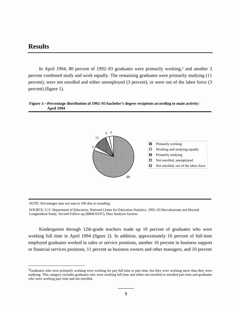
Kindergarten through 12th-grade teachers made up 10 percent of graduates who were
working full time in April 1994 (figure 2). In addition, approximately 16 percent of full-time
employed graduates worked in sales or service positions, another 16 percent in business support
or financial services positions, 11 percent as business owners and other managers, and 10 percent
3Graduates who were primarily working were working for pay full time or part time, but they were working more than they werestudying. This category includes graduates who were working full time and either not enrolled or enrolled part time and graduateswho were working part time and not enrolled.
Results
10
Figure 2—Percentage distribution of 1992–93 bachelor’s degree recipients who were employed full time Figure 2—according to occupation: April 1994
NOTE: Percentages may not sum to 100 due to rounding.
SOURCE: U.S. Department of Education, National Center for Education Statistics, 1992–93 Baccalaureate and BeyondLongitudinal Study, Second Follow-up (B&B:93/97), Data Analysis System.
1
2
4
4
6
6
7
9
10
11
16
16
10
0 2 4 6 8 10 12 14 16 18 20
Legal professionals and legal support occupations
Law enforcement occupations, military
Editors, writers, and artists
Blue collar occupations
Clerical occupations
Computer and technical occupations
Health occupations
Engineers, scientists, lab and research assistants
K–12 teachers
Other instructors and human services occupations
Business owners and other managers
Business support, financial services occupations
Sales and service occupations
Percent
K–12 teachers
as other instructors or human services professionals, such as social workers and religious leaders.
The remaining 37 percent of graduates who were employed full time worked as engineers, sci-
entists, or lab/research assistants; in health occupations; as computer or technical workers; in
clerical or blue-collar jobs; as editors, writers, or artists; in law enforcement or the military; or in
a legal occupation.
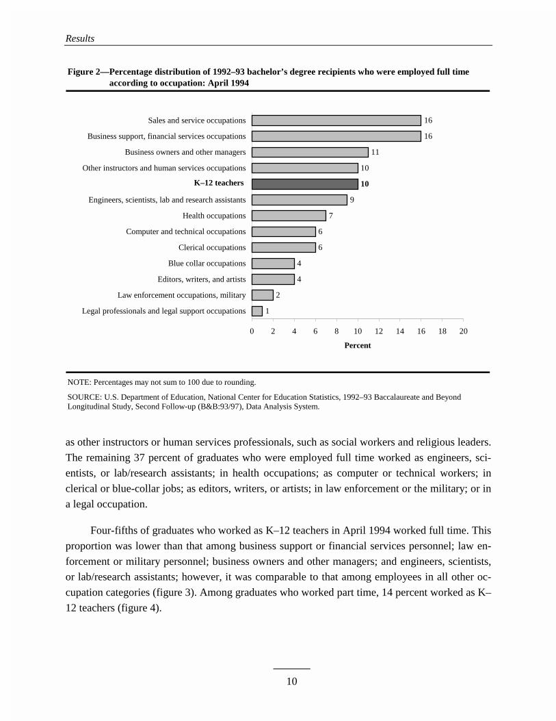
Four-fifths of graduates who worked as K–12 teachers in April 1994 worked full time. This
proportion was lower than that among business support or financial services personnel; law en-
forcement or military personnel; business owners and other managers; and engineers, scientists,
or lab/research assistants; however, it was comparable to that among employees in all other oc-
cupation categories (figure 3). Among graduates who worked part time, 14 percent worked as K–
12 teachers (figure 4).

Results
11
Figure 3—Percentage of 1992–93 bachelor’s degree recipients who were employed full time, by occupation: Figure 3—April 1994
*Statistically significantly different from K–12 teachers at the .05 level.
SOURCE: U.S. Department of Education, National Center for Education Statistics, 1992–93 Baccalaureate and BeyondLongitudinal Study, Second Follow-up (B&B:93/97), Data Analysis System.
76
76
78
78
83
83
87
90
91
91
92
96
79
0 10 20 30 40 50 60 70 80 90 100
Blue collar occupations
Other instructors and human services occupations
Clerical occupations
Sales and service occupations
K–12 teachers
Editors, writers, and artists
Health occupations
Engineers, scientists, lab and research assistants*
Legal professionals and legal support occupations
Computer and technical occupations
Business owners and other managers*
Law enforcement occupations, military*
Business support, financial services occupations*
Percent
K–12 teachers
Whether they were employed full time or part time, most graduates who worked as K–12
teachers in April 1994 were also employed in April 1997. Among those employed full time as
K–12 teachers in April 1994, 88 percent were primarily working, 3 percent were working and
studying equal amounts, 3 percent were primarily studying, 1 percent were not enrolled and un-
employed, and 4 percent were not enrolled and out of the labor force in April 1997 (figure 5).
Among those employed part time as K–12 teachers in April 1994, 85 percent were primarily
working, 5 percent were working and studying equal amounts, 3 percent were primarily study-
ing, 3 percent were not enrolled and unemployed, and 5 percent were not enrolled and out of the
labor force in April 1997.
Results
12
Figure 4—Percentage distribution of 1992–93 bachelor’s degree recipients who were employed part time Figure 4—according to occupation: April 1994
NOTE: Percentages may not sum to 100 due to rounding.
SOURCE: U.S. Department of Education, National Center for Education Statistics, 1992–93 Baccalaureate and BeyondLongitudinal Study, Second Follow-up (B&B:93/97), Data Analysis System.
1
1
3
3
4
5
6
7
7
8
17
24
14
0 5 10 15 20 25
Legal professionals and legal support occupations
Law enforcement occupations, military
Business support, financial services occupations
Computer and technical occupations
Editors, writers, artists
Business owners and other managers
Blue collar occupations
Engineers, scientists, lab and research assistants
Health occupations
Clerical occupations
K–12 teachers
Other instructors and human services occupations
Sales and service occupations
Percent
K–12 teachers
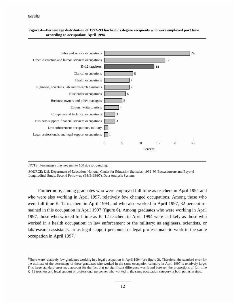
Furthermore, among graduates who were employed full time as teachers in April 1994 and
who were also working in April 1997, relatively few changed occupations. Among those who
were full-time K–12 teachers in April 1994 and who also worked in April 1997, 82 percent re-
mained in this occupation in April 1997 (figure 6). Among graduates who were working in April
1997, those who worked full time as K–12 teachers in April 1994 were as likely as those who
worked in a health occupation; in law enforcement or the military; as engineers, scientists, or
lab/research assistants; or as legal support personnel or legal professionals to work in the same
occupation in April 1997.4
4There were relatively few graduates working in a legal occupation in April 1994 (see figure 2). Therefore, the standard error forthe estimate of the percentage of these graduates who worked in the same occupation category in April 1997 is relatively large.This large standard error may account for the fact that no significant difference was found between the proportions of full-timeK–12 teachers and legal support or professional personnel who worked in the same occupation category at both points in time.
Results
13
Figure 5—Percentage distribution of 1992–93 bachelor’s degree recipients who were employed as Figure 5—K–12 teachers in April 1994 according to main activity in April 1997, by April 1994 Figure 5—employment status
NOTE: Percentages may not sum to 100 due to rounding.
SOURCE: U.S. Department of Education, National Center for Education Statistics, 1992–93 Baccalaureate and BeyondLongitudinal Study, Second Follow-up (B&B:93/97), Data Analysis System.
Full-time K–12 teachers
88
33 1 4
Part-time K–12 teachers
85
53
3 5Primarily working
Working andstudying equally
Primarily studying
Not enrolled,unemployed
Not enrolled, out ofthe labor force
In contrast, graduates who worked full time in April 1994 in any other occupation category
were less likely than full-time K–12 teachers to still be in this occupation category in April 1997.
Although one might expect such differences between K–12 teachers and clerical or blue-collar
workers, K–12 teachers were also more likely than business support/financial services personnel;
editors, writers, and artists; computer and technical workers; other instructors and human serv-
ices personnel to work in the same occupation category in both 1994 and 1997.
Somewhat fewer of those who were working part time remained in teaching. Among April
1994 part-time K–12 teachers who worked in April 1997, 67 percent worked as K–12 teachers in
April 1997 (figure 7). Among graduates who worked in April 1997, graduates who worked part
time in April 1994 as K–12 teachers were more likely than those who worked part time as com-
puter or technical workers, sales/service representatives, blue-collar workers, business owners
and other managers, or clerical workers to work in the same occupation in April 1997. In other
words, part-time K–12 teachers were as likely as graduates who worked part time in the remain-
ing occupations to work in the same occupation in both time periods.

Results
14
Figure 6—Among 1992–93 bachelor’s degree recipients who worked full time in April 1994, percentage Figure 6—who worked in the same occupation category in April 1997, by April 1994 occupation
*Statistically significantly different from K–12 teachers at the .05 level.
SOURCE: U.S. Department of Education, National Center for Education Statistics, 1992–93 Baccalaureate and BeyondLongitudinal Study, Second Follow-up (B&B:93/97), Data Analysis System.
25
39
41
45
53
55
57
61
66
71
73
83
82
0 10 20 30 40 50 60 70 80 90 100
Clerical occupations*
Blue collar occupations*
Business owners and other managers*
Sales and service occupations*
Computer and technical occupations*
Other instructors and human services occupations*
Legal professionals and legal support occupations
Editors, writers, and artists*
Business support, financial services occupations*
Engineers, scientists, lab and research assistants
Law enforcement occupations, military
K–12 teachers
Health occupations
Percent
K–12 teachers
Thus, 1992–93 college graduates who worked as K–12 teachers in April 1994 were less
likely than graduates in many other occupation categories to be working in another occupation,
studying primarily, not enrolled and unemployed, or not enrolled and out of the labor force in
April 1997. However, this analysis examines graduates’ activities and occupations at only two
points in time: April 1994 and April 1997. Graduates who had taught in April 1994 may have
been more likely than graduates in other occupations to leave teaching after April 1994—in order
to work toward a teaching certificate or master’s degree, for example—and return by April 1997.
The data illustrate this point to some degree. Among graduates who were primarily working and
employed full time in April 1994, those who worked as K–12 teachers were more likely than

Results
15
Figure 7—Among 1992–93 bachelor’s degree recipients who worked part time in April 1994, percentage Figure 7—who worked in the same occupation category in April 1997, by April 1994 occupation
*Statistically significantly different from K–12 teachers at the .05 level.
NOTE: Too few sample members worked part time in law enforcement, the military, or a legal profession to produce reliable estimates for these categories.
SOURCE: U.S. Department of Education, National Center for Education Statistics, 1992–93 Baccalaureate and BeyondLongitudinal Study, Second Follow-up (B&B:93/97), Data Analysis System.
10
23
24
27
27
43
43
45
56
80
67
0 10 20 30 40 50 60 70 80 90 100
Clerical occupations*
Business owners and other managers*
Blue collar occupations*
Sales and service occupations*
Computer and technical occupations*
Editors, writers, and artists
Engineers, scientists, lab and research assistants
Other instructors and human services occupations
Business support, financial services occupations
K–12 teachers
Health occupations
Percent
K–12 teachers
most others to have enrolled at any postsecondary or graduate level between completing the
1992–93 bachelor’s degree and April 1997 (figure 8).5 Such higher rates of postsecondary en-
rollment among teachers may reflect school district salary schedules, which commonly reward
teachers for earning postsecondary education units.6
Finally, in addition to perceptions that the overall new teacher attrition rate is high, policy-
makers and researchers fear that, among teachers, those who major in fields other than education,
particularly mathematics and the natural sciences, are more likely than education majors to leave
5Elementary/secondary teaching graduates were no more likely than graduates who worked full time in April 1994 as other in-structors or human services personnel or those in legal occupations to enroll at either level after completing the bachelor’s degree.6These data do not completely address the question of whether new teachers were more likely than those in other occupations toleave and return within the three year period between April 1994 and April 1997. Those who did enroll at a postsecondary insti-tution, as well as those who did not, may have continued working in their April 1994 occupation, changed occupations, orstopped working completely for any or all of the period between April 1994 and April 1997.

Results
16
Figure 8—Among 1992–93 bachelor’s degree recipients who were primarily working and employed full Figure 8—time in April 1994, percentages who had enrolled at the postsecondary and at the graduate levels Figure 8—by April 1997, by April 1994 occupation
**Both estimates statistically significantly different from K–12 teachers at the .05 level.
SOURCE: U.S. Department of Education, National Center for Education Statistics, 1992–93 Baccalaureate and BeyondLongitudinal Study, Second Follow-up (B&B:93/97), Data Analysis System.
14
14
15
14
16
18
24
23
22
26
36
32
28
30
30
30
31
35
38
39
40
46
49
54
4264
0 10 20 30 40 50 60 70 80 90 100
Editors, writers, and artists**
Business owners and other managers**
Sales and service occupations**
Blue collar occupations**
Business support, financial services occupations**
Computer and technical occupations**
Health occupations**
Clerical occupations**
Law enforcement occupations, military**
Engineers, scientists, lab and research assistants**
Legal professionals and legal support occupations
Other instructors and human services occupations
K–12 teachers
Percent
Any postsecondary enrollment
Any graduate enrollment
K–12 teachers
the profession. The B&B:93/97 data indicate there was no difference between teachers who ma-
jored in education and those who majored in engineering, mathematics or the natural sciences in
the proportion who were primarily working in April 1997 (figure 9). However, among graduates
who worked as K–12 teachers in April 1994 and who were working in April 1997, 70 percent of
those who had majored in engineering, mathematics, or the natural sciences were teaching at the
K–12 level in April 1997, compared with 86 percent of education majors (figure 10).
Results
17
Figure 9—Among 1992–93 bachelor’s degree recipients who taught at the K–12 level in April 1994, Figure 9—percentage distribution according to main activity in April 1997, by undergraduate major
NOTE: Percentages may not sum to 100 due to rounding.
SOURCE: U.S. Department of Education, National Center for Education Statistics, 1992–93 Baccalaureate and BeyondLongitudinal Study, Second Follow-up (B&B:93/97), Data Analysis System.
818690
33
6
925
1 03
4 25
0
10
20
30
40
50
60
70
80
90
100
Education Engineering,mathematics, ornatural sciences
Other
Percent
Out of the labor force
Unemployed
Primarily student
Equal parts study and work
Primarily working
4
21
2
3
0 5
53
Thus, this analysis indicates that among 1992–93 college graduates who worked in April
1994, approximately a year after they had completed their bachelor’s degrees, those who taught
at the K–12 level were among the least likely of all employed graduates to work in a different
profession 3 years later. Relatively few K–12 teaching graduates had different main activities or
different occupations in April 1997 than they did in April 1994. Attrition rates among teachers
varied with major, however: April 1994 K–12 teaching graduates who had majored in engineer-
ing, mathematics, or the natural sciences were less likely than those who had majored in educa-
tion to be teaching in April 1997.
Results
18
Figure 10—Among 1992–93 bachelor’s degree recipients who taught at the K–12 level in April 1994 andFigure 10—who were working in April 1997, percentage who worked as K–12 teachers in April 1997, by Figure 10—undergraduate major
SOURCE: U.S. Department of Education, National Center for Education Statistics, 1992–93 Baccalaureate and BeyondLongitudinal Study, Second Follow-up (B&B:93/97), Data Analysis System.
86
7062
0
20
40
60
80
100
Education Engineering, mathematics,or natural sciences
Other
Percent
The remainder of this report examines whether two additional variables—graduates’ per-
ceptions of how their postsecondary fields of study were related to their occupations and their
views about the professional status of their occupations—vary with occupations and are associ-
ated with changing occupations between April 1994 and April 1997.
Relationship Between April Occupations and Postsecondary Fields of Study
Among those working as K–12 teachers in April 1994, nearly all reported that their jobs
were related to their undergraduate field of study (97 percent among full-time teachers and 96
percent among part-time teachers) (figure 11). Similarly, most graduates who worked either full
time or part time in a health occupation or as engineers, scientists, or lab/research assistants indi-
cated that their jobs were related to their undergraduate major.
Graduates who worked in other occupations in April 1994 were considerably less likely to
report that their jobs were related to their undergraduate majors. As one might expect, graduates
who worked full time or part time in clerical, blue-collar, or sales or service occupations were
less likely than teachers to report that their jobs were related to their undergraduate majors: 62
percent or less of graduates in these occupations did so. In addition, both full- and part-time
business owners and other managers were less likely than teachers to report that their jobs were
related to their undergraduate fields of study. Likewise, among full-time employees, other in-
structors or human services personnel (88 percent) and business support or financial services
Results
19
Figure 11—Percentage of 1992–93 bachelor’s degree recipients who reported that their job was related toFigure 11—their undergraduate field of study, by employment status and occupation: April 1994
*Full-time estimate statistically significantly different from K–12 teachers at the .05 level.**Both estimates statistically significantly different from K–12 teachers at the .05 level.†Sample size too small for a reliable estimate.
SOURCE: U.S. Department of Education, National Center for Education Statistics, 1992–93 Baccalaureate and BeyondLongitudinal Study, Second Follow-up (B&B:93/97), Data Analysis System.
33
20
26
54
72
67
87
79
96
88
40
41
62
72
76
76
81
81
88
89
94
95
96
†
†
97
0 10 20 30 40 50 60 70 80 90 100
Clerical occupations**
Blue collar occupations**
Sales and service occupations**
Business owners and other managers**
Law enforcement occupations, military*
Legal professionals and legal support occupations
Business support, financial services occupations*
Computer and technical occupations*
Other instructors and human services occupations*
Editors, writers, and artists
Engineers, scientists, lab and research assistants
Health occupations
K–12 teachers
Percent
Employed full time
Employed part time
K–12 teachers
personnel and computer/technical workers (81 percent each) were less likely than teachers to re-
port that their jobs were related to their undergraduate fields of study.
Among graduates who were working full time in April 1997, 93 percent of K–12 teachers
reported that their jobs were somewhat or closely related to their graduate or undergraduate
fields of study, a proportion similar to that among those working full time as an engineer, scien-
tist, or lab/research assistant (93 percent) or in a health occupation (92 percent) (figure 12). In
April 1997, full-time K–12 teachers among 1992–93 college graduates were more likely than
Results
20
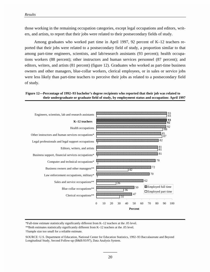
those working in the remaining occupation categories, except legal occupations and editors, writ-
ers, and artists, to report that their jobs were related to their postsecondary fields of study.
Among graduates who worked part time in April 1997, 92 percent of K–12 teachers re-
ported that their jobs were related to a postsecondary field of study, a proportion similar to that
among part-time engineers, scientists, and lab/research assistants (93 percent); health occupa-
tions workers (88 percent); other instructors and human services personnel (87 percent); and
editors, writers, and artists (81 percent) (figure 12). Graduates who worked as part-time business
owners and other managers, blue-collar workers, clerical employees, or in sales or service jobs
were less likely than part-time teachers to perceive their jobs as related to a postsecondary field
of study.
Figure 12—Percentage of 1992–93 bachelor’s degree recipients who reported that their job was related toFigure 12—their undergraduate or graduate field of study, by employment status and occupation: April 1997
*Full-time estimate statistically significantly different from K–12 teachers at the .05 level.**Both estimates statistically significantly different from K–12 teachers at the .05 level.†Sample size too small for a reliable estimate.
SOURCE: U.S. Department of Education, National Center for Education Statistics, 1992–93 Baccalaureate and BeyondLongitudinal Study, Second Follow-up (B&B:93/97), Data Analysis System.
31
36
26
42
81
87
88
93
47
50
62
70
72
78
81
81
82
85
92
93
†
†
†
†
9293
0 10 20 30 40 50 60 70 80 90 100
Clerical occupations**
Blue collar occupations**
Sales and service occupations**
Law enforcement occupations, military*
Business owners and other managers**
Computer and technical occupations*
Business support, financial services occupations*
Editors, writers, and artists
Legal professionals and legal support occupations
Other instructors and human services occupations*
Health occupations
K–12 teachers
Engineers, scientists, lab and research assistants
Percent
Employed full time
Employed part time
K–12 teachers

Results
21
To assess whether graduates who perceived their 1994 occupations to be related to their
undergraduate fields of study were more likely to work in a different occupation in April 1997, a
new variable was created to measure occupation change. This variable compared the April 1994
occupation category with that in April 1997: if the two were identical, the graduate was defined
as “not having changed occupations.” The variable also took into consideration that in many oc-
cupational areas, employees may change occupations but remain in a career path within a field.
For example, if in April 1994 a graduate worked as a research assistant, and in April 1997 as a
scientist or researcher, that graduate was defined as “not having changed occupation.” Similarly,
graduates whose April 1994 occupation was classified as business support or financial services
and whose April 1997 occupation was classified as financial services professional were defined
as “not having changed occupation.” However, K–12 teachers were required to fall in the same
occupation category at both points in time to be defined as “not having changed occupation.”
Appendix A provides more detail about which combinations of occupation categories were de-
fined as “changes.”
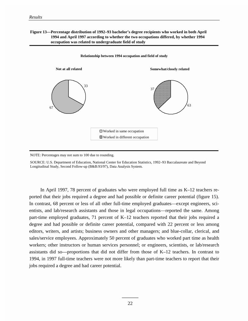
Compared with those who reported that their April 1994 occupations were not at all related
to their undergraduate fields of study, graduates who reported that their 1994 occupations were
somewhat or closely related were considerably less likely to work in a different occupation in
April 1997. Whereas 37 percent of graduates with jobs related to their field of study worked in a
different occupation 3 years later, 67 percent of those with unrelated jobs did so (figure 13).
Professional Status of April Occupations
Four-fifths of graduates who worked as full-time K–12 teachers in April 1994 believed
their teaching job both required a bachelor’s degree and had possible or definite career potential
(figure 14). Although a similar proportion (79 percent) of graduates who worked full time as en-
gineers, scientists, and lab/research assistants perceived their jobs as having similar professional
status, graduates who worked full time in all other occupation categories were less likely to share
that perception.
Part-time teachers among graduates were less likely than their full-time counterparts to rate
their jobs as both requiring a degree and having career potential. However, 64 percent of part-
time teachers did so, a higher proportion than among graduates working part time as other in-
structors or human services personnel; editors, writers, and artists; computer/technical workers;
business owners and other managers; clerical and blue-collar workers; and sales/service people.
Results
22
Figure 13—Percentage distribution of 1992–93 bachelor’s degree recipients who worked in both April Figure 14—1994 and April 1997 according to whether the two occupations differed, by whether 1994Figure 14—occupation was related to undergraduate field of study
NOTE: Percentages may not sum to 100 due to rounding.
SOURCE: U.S. Department of Education, National Center for Education Statistics, 1992–93 Baccalaureate and BeyondLongitudinal Study, Second Follow-up (B&B:93/97), Data Analysis System.
Relationship between 1994 occupation and field of study
Not at all related
33
67
Somewhat/closely related
63
37
Worked in same occupation
Worked in different occupation
In April 1997, 78 percent of graduates who were employed full time as K–12 teachers re-
ported that their jobs required a degree and had possible or definite career potential (figure 15).
In contrast, 68 percent or less of all other full-time employed graduates—except engineers, sci-
entists, and lab/research assistants and those in legal occupations—reported the same. Among
part-time employed graduates, 71 percent of K–12 teachers reported that their jobs required a
degree and had possible or definite career potential, compared with 22 percent or less among
editors, writers, and artists; business owners and other managers; and blue-collar, clerical, and
sales/service employees. Approximately 50 percent of graduates who worked part time as health
workers; other instructors or human services personnel; or engineers, scientists, or lab/research
assistants did so—proportions that did not differ from those of K–12 teachers. In contrast to
1994, in 1997 full-time teachers were not more likely than part-time teachers to report that their
jobs required a degree and had career potential.

Results
23
Figure 14—Percentage of 1992–93 bachelor’s degree recipients who reported that their job had careerFigure 15—potential and that a bachelor’s degree was required to obtain the job, by employment status andFigure 15—occupation: April 1994
*Full-time estimate statistically significantly different from K–12 teachers at the .05 level.**Both estimates statistically significantly different from K–12 teachers at the .05 level.†Sample size too small for a reliable estimate.
SOURCE: U.S. Department of Education, National Center for Education Statistics, 1992–93 Baccalaureate and BeyondLongitudinal Study, Second Follow-up (B&B:93/97), Data Analysis System.
5
6
10
3
38
16
26
14
44
50
9
16
33
34
36
39
50
54
57
57
62
79
†
†
6482
0 10 20 30 40 50 60 70 80 90 100
Blue collar occupations**
Clerical occupations**
Legal professionals and legal support occupations*
Business owners and other managers**
Sales and service occupations**
Law enforcement occupations, military*
Other instructors and human services occupations**
Editors, writers, and artists**
Business support, financial services occupations*
Computer and technical occupations**
Health occupations*
Engineers, scientists, lab and research assistants
K–12 teachers
Percent
Employed full time
Employed part time
K–12 teachers
As one might expect, graduates who perceived their April 1994 occupations as requiring a
degree and having career potential were less likely than those who perceived otherwise to be
working in a different occupation in April 1997. Among graduates who worked in April of both
1994 and 1997, 32 percent of those who reported that their April 1994 jobs required a degree and
had career potential were working in a different occupation in April 1997 (figure 16). In contrast,
71 percent of those who reported that their 1994 job did not require a degree and did not have
career potential worked in a different occupation 3 years later.

Results
24
Figure 15—Percentage of 1992–93 bachelor’s degree recipients who reported that their job had careerFigure 16—potential and that a bachelor’s degree was required to obtain the job, by employment status andFigure 16—occupation: April 1997
*Full-time estimate statistically significantly different from K–12 teachers at the .05 level.**Both estimates statistically significantly different from K–12 teachers at the .05 level.†Sample size too small for a reliable estimate.
SOURCE: U.S. Department of Education, National Center for Education Statistics, 1992–93 Baccalaureate and BeyondLongitudinal Study, Second Follow-up (B&B:93/97), Data Analysis System.
11
7
11
2
22
50
49
52
19
30
42
42
45
55
62
63
66
68
70
81
71
†
†
†
†
78
0 10 20 30 40 50 60 70 80 90 100
Blue collar occupations**
Clerical occupations**
Law enforcement occupations, military*
Business owners and other managers**
Sales and service occupations**
Editors, writers, and artists**
Other instructors and human services occupations*
Computer and technical occupations*
Business support, financial services occupations*
Health occupations*
Legal professionals and legal support occupations
K–12 teachers
Engineers, scientists, lab and research assistants
Percent
Employed full time
Employed part time
K–12 teachers
Changing Occupations: Multivariate Analysis
The bivariate results discussed thus far indicate that many of the variables examined are
related to each other as well as to the probability of graduates’ changing occupations between
April 1994 and April 1997. Rates of change were related to graduates’ 1994 occupations, their
perceptions of their jobs’ professional status and relationship to their postsecondary fields of
study. Graduates’ perceptions also were related to their occupations. Multivariate techniques al-
low researchers to disentangle some of this covariation.
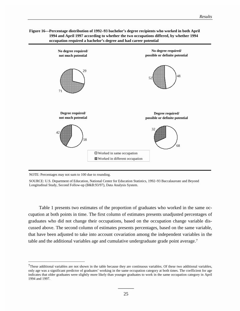
Results
25
Figure 16—Percentage distribution of 1992–93 bachelor’s degree recipients who worked in both April Figure 17—1994 and April 1997 according to whether the two occupations differed, by whether 1994Figure 17—occupation required a bachelor’s degree and had career potential
NOTE: Percentages may not sum to 100 due to rounding.
SOURCE: U.S. Department of Education, National Center for Education Statistics, 1992–93 Baccalaureate and BeyondLongitudinal Study, Second Follow-up (B&B:93/97), Data Analysis System.
No degree required/possible or definite potential
4852
No degree required/not much potential
29
71
Degree required/possible or definite potential
68
32
Degree required/not much potential
58
42
Worked in same occupation
Worked in different occupation
Degree required/possible or definite potential
Table 1 presents two estimates of the proportion of graduates who worked in the same oc-
cupation at both points in time. The first column of estimates presents unadjusted percentages of
graduates who did not change their occupations, based on the occupation change variable dis-
cussed above. The second column of estimates presents percentages, based on the same variable,
that have been adjusted to take into account covariation among the independent variables in the
table and the additional variables age and cumulative undergraduate grade point average.7
7These additional variables are not shown in the table because they are continuous variables. Of these two additional variables,only age was a significant predictor of graduates’ working in the same occupation category at both times. The coefficient for ageindicates that older graduates were slightly more likely than younger graduates to work in the same occupation category in April1994 and 1997.
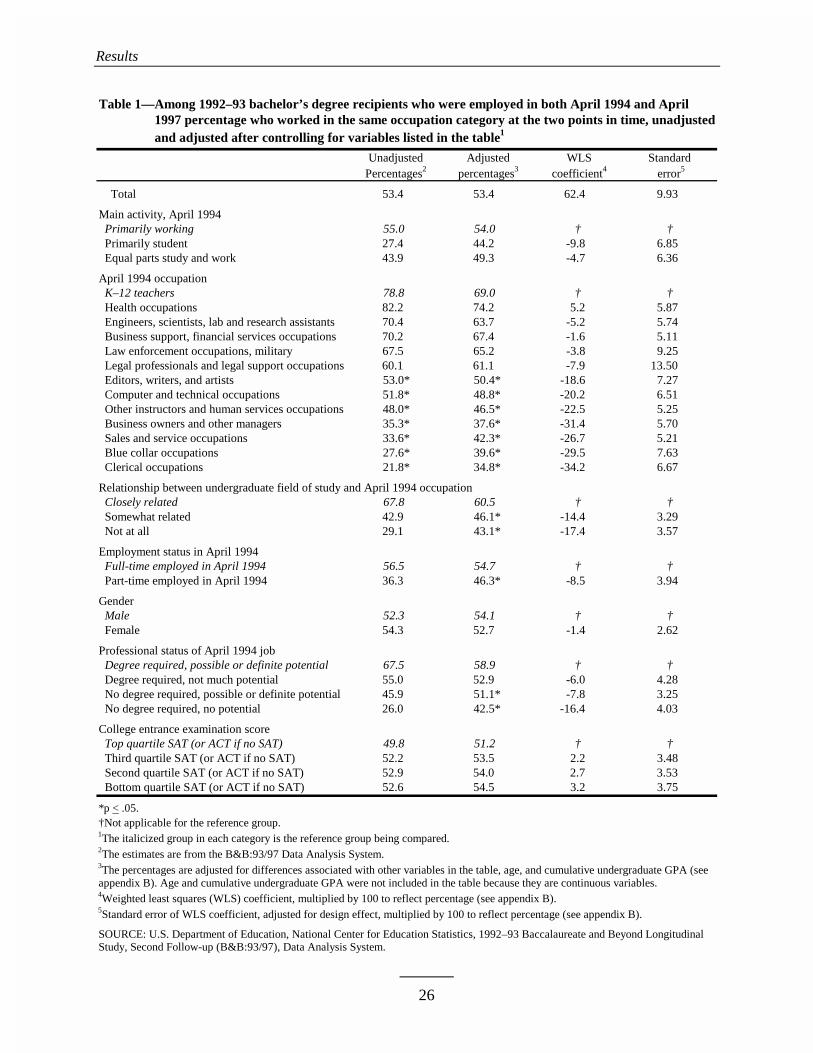
Results
26
Table 1—Among 1992–93 bachelor’s degree recipients who were employed in both April 1994 and AprilTable 1—1997 percentage who worked in the same occupation category at the two points in time, unadjustedTable 1—and adjusted after controlling for variables listed in the table1
Unadjusted Adjusted WLS Standard Percentages2 percentages3 coefficient4 error5
Total 53.4 53.4 62.4 9.93
Main activity, April 1994 Primarily working 55.0 54.0 † † Primarily student 27.4 44.2 -9.8 6.85 Equal parts study and work 43.9 49.3 -4.7 6.36
April 1994 occupation K–12 teachers 78.8 69.0 † † Health occupations 82.2 74.2 5.2 5.87 Engineers, scientists, lab and research assistants 70.4 63.7 -5.2 5.74 Business support, financial services occupations 70.2 67.4 -1.6 5.11 Law enforcement occupations, military 67.5 65.2 -3.8 9.25 Legal professionals and legal support occupations 60.1 61.1 -7.9 13.50 Editors, writers, and artists 53.0* 50.4* -18.6 7.27 Computer and technical occupations 51.8* 48.8* -20.2 6.51 Other instructors and human services occupations 48.0* 46.5* -22.5 5.25 Business owners and other managers 35.3* 37.6* -31.4 5.70 Sales and service occupations 33.6* 42.3* -26.7 5.21 Blue collar occupations 27.6* 39.6* -29.5 7.63 Clerical occupations 21.8* 34.8* -34.2 6.67
Relationship between undergraduate field of study and April 1994 occupation Closely related 67.8 60.5 † † Somewhat related 42.9 46.1* -14.4 3.29 Not at all 29.1 43.1* -17.4 3.57
Employment status in April 1994 Full-time employed in April 1994 56.5 54.7 † † Part-time employed in April 1994 36.3 46.3* -8.5 3.94
Gender Male 52.3 54.1 † † Female 54.3 52.7 -1.4 2.62
Professional status of April 1994 job Degree required, possible or definite potential 67.5 58.9 † † Degree required, not much potential 55.0 52.9 -6.0 4.28 No degree required, possible or definite potential 45.9 51.1* -7.8 3.25 No degree required, no potential 26.0 42.5* -16.4 4.03
College entrance examination score Top quartile SAT (or ACT if no SAT) 49.8 51.2 † † Third quartile SAT (or ACT if no SAT) 52.2 53.5 2.2 3.48 Second quartile SAT (or ACT if no SAT) 52.9 54.0 2.7 3.53 Bottom quartile SAT (or ACT if no SAT) 52.6 54.5 3.2 3.75
*p < .05.†Not applicable for the reference group.1The italicized group in each category is the reference group being compared.2The estimates are from the B&B:93/97 Data Analysis System.3The percentages are adjusted for differences associated with other variables in the table, age, and cumulative undergraduate GPA (seeappendix B). Age and cumulative undergraduate GPA were not included in the table because they are continuous variables.4Weighted least squares (WLS) coefficient, multiplied by 100 to reflect percentage (see appendix B).5Standard error of WLS coefficient, adjusted for design effect, multiplied by 100 to reflect percentage (see appendix B).
SOURCE: U.S. Department of Education, National Center for Education Statistics, 1992–93 Baccalaureate and Beyond LongitudinalStudy, Second Follow-up (B&B:93/97), Data Analysis System.

Results
27
After controlling for the other variables in the model, graduates who taught in April 1994
were as likely to be teaching in April 1997 as graduates who worked in most other professions
were not to change occupations. Graduates who worked in health occupations; in business sup-
port/financial services occupations; in law enforcement and the military; as engineers, scientists,
and lab/research assistants; and legal occupations in 1994 were no more likely than teachers to
be working in their occupation categories in 1997 as well. In fact, no occupation category was
more stable than teachers.
Graduates’ perceptions of their April 1994 job’s professional status and of the relationship
between their undergraduate field of study and their April 1994 job were, independently, related
to whether they worked in the same occupation category at both points in time. Graduates who
perceived their April 1994 job as unrelated or somewhat related to their undergraduate major
field of study were less likely than those who perceived a close relationship to work in the same
occupation in 1997 as in 1994. Compared with graduates who reported that a degree was not re-
quired to obtain their April 1994 job, graduates who reported that a degree was required were
more likely to work in the same occupation category at both points in time. However, graduates’
perceptions of the career potential of their jobs appeared not to make a difference.
In addition to these variables related to the type of job graduates were doing, their em-
ployment status was associated with the likelihood that they changed occupations, after adjusting
for covariation of employment status with the remaining variables in the model. Graduates who
worked full time in April 1994 were more likely than part-time employees to work in the same
occupation category in April 1997. However, whether graduates were primarily working, com-
bining work and study equally, or primarily studying in April 1994 was not associated with
working in the same occupation category in April 1997.

THIS PAGE INTENTIONALLY LEFT BLANK

29
Conclusion
Concern about K–12 teacher shortages has raised questions regarding the attrition rate
among teachers, and particularly new teachers. This analysis examined whether 1992–93 bache-
lor’s degree recipients who taught at the elementary/secondary level in 1994 were less likely to
work in the same occupation in 1997, compared with their peers in other occupations. The data
indicate that K–12 teachers among 1992–93 college graduates were among the least likely to
work in different occupations in 1997 compared with 1994.
Among graduates who were employed in April 1994 and April 1997, K–12 teachers (i.e.,
graduates who taught in 1994) were as likely as graduates who worked in other white collar, pro-
fessional occupations to work in the same occupation category in April 1997. Specifically, ap-
proximately four-fifths of graduates who taught in April 1994 were also teaching in April 1997,
and similar proportions of graduates who worked as health occupations professionals; engineers,
scientists, lab/research assistants; in legal occupations; in law enforcement or the military; or as
business support/financial services workers worked in their respective occupation categories in
both April 1994 and April 1997. Graduates who worked in other occupation categories in April
1994 were less likely than K–12 teachers to work in the same occupation category at both points
in time.
Moreover, this result occurred in spite of the fact that teachers were held to a higher stan-
dard. Teachers were defined as not changing occupations if they worked as K–12 teachers at
both points in time, whereas graduates who worked in other occupations were defined as not
changing occupations if they worked in the same occupation categories or, in some cases, related
occupation categories.
Those who taught at the K–12 level part time in April 1994 were less likely than their full-
time counterparts also to work as K–12 teachers in April 1997. Nevertheless, among part-time
workers in April 1994, K–12 teachers were among the most likely of all occupation categories to
work in the same occupation category in April 1997 as in April 1994.
Graduates’ perceptions of whether their April 1994 occupations were closely related to
their undergraduate field of study and of the professional status of the April 1994 occupation
were related to whether they worked in the same occupation category in both April 1994 and
April 1997. Graduates who reported that their April 1994 occupations were somewhat or closely

Conclusion
30
related to their undergraduate fields of study were considerably less likely than those who re-
ported that their 1994 occupations were not at all related to work in a different occupation cate-
gory in April 1997. As one might expect, graduates who perceived their April 1994 occupations
as having professional status, defined as requiring a degree and having career potential, were less
likely than those who perceived otherwise to be working in a different occupation in April 1997.
Consistent with these findings, in both 1994 and 1997, 1992–93 college graduates who worked
as K–12 teachers were highly likely to report that their jobs were related to their postsecondary
fields of study and had professional status.
There are several points to keep in mind regarding the major finding of this report: K–12
teachers were among the least likely of 1992–93 bachelor’s degree recipients to change occupa-
tions between April 1994 and April 1997. First, the estimates regarding occupation attrition that
are presented in this report include only those graduates who worked in April 1994 and April
1997. Therefore, they do not take into account attrition from particular occupations in April 1994
to nonwork (e.g., studying or child rearing) in April 1997. However, as the analysis of main ac-
tivity changes between 1994 and 1997 demonstrates, most graduates, including those who
worked as K–12 teachers, did work in both April 1994 and 1997. Consequently, these estimates
are not likely to vary much from estimates that do take into account departures from the work
force as well as changes in occupation.
Second, although the estimates of attrition among new teachers reported here appear to be
lower than many discussed among policymakers and in news reports, there are many potential
reasons for such differences. These data do not represent all new teachers in April 1994, but only
new teachers among 1992–93 bachelor’s degree recipients. Given independent estimates of the
proportion of teachers who are new college graduates, this group is likely to represent between
one-half and two-thirds of all first-time teachers in April 1994. Therefore, many new teachers in
April 1994 (i.e., those who received their bachelor’s degrees before July 1992) are omitted from
the analysis.
Third, these results must also be interpreted in the context of labor market conditions of the
mid 1990s and other influences associated with this point in time. For example, data from 1999–
2000 graduates might support quite different findings, given the booming economy and the po-
tential for new college graduates to earn relatively large salaries in technology related occupa-
tions.
Fourth, this analysis is limited to two points in time, and does not take into account stop-
ping out behavior between April 1994 and April 1997. Such behavior may vary among graduates
Conclusion
31
in different occupations, and also may account for differences between these attrition rates and
others calculated over different periods of time in a graduate’s career.
Finally, this report discusses attrition from graduates’ April 1994 occupations, and not
turnover within those occupations. Turnover among jobs within occupations may vary among
occupations in different ways than attrition does. For example, although K–12 teachers among
recent college graduates have relatively low attrition rates, they may have relatively high turn-
over rates compared with their classmates in other occupations. High turnover rates would also
have policy implications for schools and districts, particularly if some schools were more likely
than others to have high turnover rates among new teachers.
In sum, the point of the analysis is not to estimate the proportion of new teachers who
changed occupations but to examine their attrition rates relative to that of other college graduates
who are at similar points in their careers but in different occupations. In that regard, the analysis
indicates that college graduates who teach soon after completing their degrees are among the
most stable in terms of occupational choice. Many new graduates did work in different occupa-
tions 4 years after completing their degrees compared with their occupation 1 year after comple-
tion. However, those who were teaching at the 1-year point were less likely, as were others in
occupations that required bachelor’s degrees, had career potential, and were related to graduates’
fields of study, to change their professions than were those in other occupations.

THIS PAGE INTENTIONALLY LEFT BLANK

33
References
Archer, J. (1999). New Teachers Abandon Field at High Rate. Education Week, 18(27): 1, 20–21.
Archibold, R.C. (1999, August 22). Worst Schools Still Seeking 400 Teachers. The New YorkTimes.
Baker, D.P., and Smith, T. (1997). Trend 2: Teacher Turnover and Teacher Quality: Refocusingthe Issue. Teachers College Record, 99: 29–35.
Bradley, A. (1999). States’ Uneven Teacher Supply Complicates Staffing of Schools. EducationWeek, 18(26): 1, 10–11.
Broughman, S.P. and Rollefson, M.R. (2000). Teacher Supply in the U.S.: Sources of NewlyHired Teachers in Public and Private Schools, 1987–88 to 1993–94 (NCES 2000–309).U.S. Department of Education, National Center for Education Statistics. Washington, DC:U.S. Government Printing Office.
Cooperman, S. (2000, January 26). The Sky Is Not Falling!: There’s a Well-Traveled Route toSolving Our Teacher Shortage. Education Week, 19(20): 31.
Darling-Hammond, L. (1984). Beyond the Commission Reports: The Coming Crisis in Teach-ing. Santa Monica, CA: RAND Corporation.
Gerald, D.E., and Hussar, W.J. (2000). Projections of Education Statistics to 2010 (NCES 2000–071). U.S. Department of Education, National Center for Education Statistics. Washington,DC: U.S. Government Printing Office.
Goodnough, A. (2000, January 21). Union Says Poll of Teachers Predicts Wave of Retirements.The New York Times.
Grissmer, D., and Kirby, S.N. (1997). Teacher Turnover and Teacher Quality. Teachers CollegeRecord, 99: 45–56.
Henke, R.R., Choy, S.P., Chen, X., Geis, S., and Alt, M.N. (1997). America’s Teachers: Profileof a Profession, 1993–94 (NCES 97–460). U.S. Department of Education, National Centerfor Education Statistics. Washington, DC: U.S. Government Printing Office.
Henke, R.R., Choy, S.P., Geis, S., and Broughman, S.P. (1996). Schools and Staffing in theUnited States: A Statistical Profile, 1993–94 (NCES 96–124). U.S. Department of Educa-

References
34
tion, National Center for Education Statistics. Washington, DC: U.S. Government PrintingOffice.
Holmes Group. (1986). Tomorrow’s Teachers. East Lansing, MI: Author.
Johnson, S.M. (2001). Can Professional Certification for Teachers Reshape Teaching as aCareer? Phi Delta Kappan, 82(5): 393–399.
Kanstoroom, M. and Finn, C.E. Jr. (Eds.) (1999). Better Teachers, Better Schools. Washington,DC: Fordham Foundation.
Murnane, R.J., Singer, J.D., Willett, J.B., Kemple, J.J., and Olson, R.J. (1991). Who Will Teach?Policies That Matter. Cambridge, MA: Harvard University Press.
National Commission on Teaching and America’s Future (NCTAF). (1996). What Matters Most:Teaching for America’s Future. New York: Author.
National Commission on Teaching and America’s Future (NCTAF). (1997). Doing What Mat-ters Most: Investing in Quality Teaching. New York: Author.
Sack, J. (1999). All Classes of Spec. Ed. Teachers in Demand Throughout Nation. EducationWeek, 18(28): 1.
Steinberg, J. (1999, August 31). As Students Return, Schools Cope with Severe Shortages ofTeachers. The New York Times.
Whitener, S.D., Gruber, K.J., Lynch, H., Tingos, K., Perona, M., and Fondelier, S. (1997). Char-acteristics of Stayers, Movers, and Leavers: Results From the Teacher Followup Survey:1994–95 (NCES 97–450). U.S. Department of Education, National Center for EducationStatistics. Washington, DC: U.S. Government Printing Office.
Wilgoren, D. (1999, July 22). Area Schools Struggle to Fill Teaching Jobs. The WashingtonPost, p. A01.
Zehr, M.A. (1998a, September 30). Voc. Ed. Administrators Troubled by Lack of CertifiedTeachers. Education Week, 18(4): 8.
Zehr, M.A. (1998b, October 28). Shortage of Consumer Sciences Teachers Hitting Home. Edu-cation Week, 18(9): 7.
35
Appendix A—Glossary
This glossary describes the variables used in this report. The variables were taken directly from the B&B:1993/1997Data Analysis System (DAS), an NCES software application that generates tables from the B&B:1993/1997 data. Adescription of the DAS software can be found in appendix B.
In the index below, the variables are organized by general topic and, within topic, listed in alphabetical order byvariable name (displayed in capital letters to the right of the label). All variable names beginning with B2 are basedon data collected in 1997.
GLOSSARY INDEX
Graduates’ CharacteristicsMain activity April 1994 .................................ACT94Main activity April 1997 .................................ACT97Age as of 12/31/94...............................................AGEHighest enrollment after bachelor’s........ B2HENPRGBachelor’s degree major ...........................BAMAJORPanel weight for NPSAS and B&B ........BNBPANELGender .........................................................GENDERCumulative undergraduate grade point average............................................GPACollege entrance examination scores ..... SATACTQ2
Employment CharacteristicsApril 1994 occupational code revised.....AJOBOCCRRelationship between April 1994 job and 1994 field of study ..........................AJOBRELTApril 1997 occupational code revised........ B2AJOBRRelationship between April 1997 job and 1994 field of study ...........................B2AJRELTEmployment status April 1994 ................. B2EM9404Employment status April 1997 ................. B2EM9704Occupational change................................ OCHANGEProfessional status of April 1994 job....... PROSTA94Professional status of April 1997 job....... PROSTA97
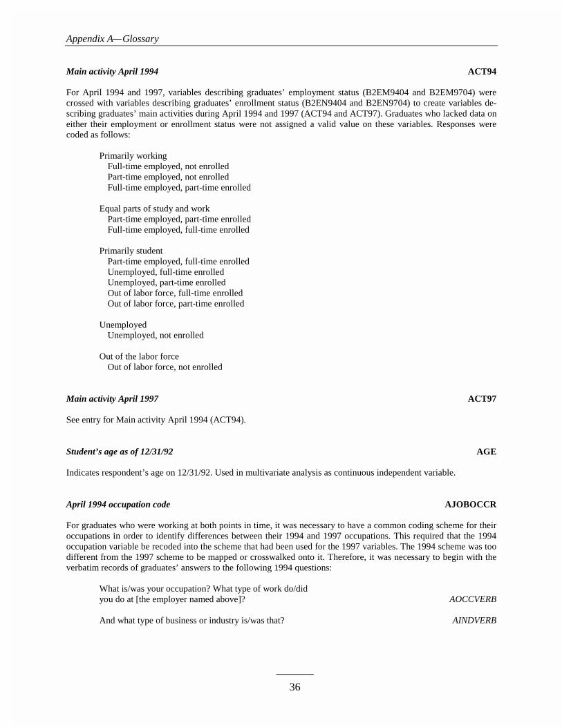
Appendix A—Glossary
36
Main activity April 1994 ACT94
For April 1994 and 1997, variables describing graduates’ employment status (B2EM9404 and B2EM9704) werecrossed with variables describing graduates’ enrollment status (B2EN9404 and B2EN9704) to create variables de-scribing graduates’ main activities during April 1994 and 1997 (ACT94 and ACT97). Graduates who lacked data oneither their employment or enrollment status were not assigned a valid value on these variables. Responses werecoded as follows:
Primarily workingFull-time employed, not enrolledPart-time employed, not enrolledFull-time employed, part-time enrolled
Equal parts of study and workPart-time employed, part-time enrolledFull-time employed, full-time enrolled
Primarily studentPart-time employed, full-time enrolledUnemployed, full-time enrolledUnemployed, part-time enrolledOut of labor force, full-time enrolledOut of labor force, part-time enrolled
UnemployedUnemployed, not enrolled
Out of the labor forceOut of labor force, not enrolled
Main activity April 1997 ACT97
See entry for Main activity April 1994 (ACT94).
Student’s age as of 12/31/92 AGE
Indicates respondent’s age on 12/31/92. Used in multivariate analysis as continuous independent variable.
April 1994 occupation code AJOBOCCR
For graduates who were working at both points in time, it was necessary to have a common coding scheme for theiroccupations in order to identify differences between their 1994 and 1997 occupations. This required that the 1994occupation variable be recoded into the scheme that had been used for the 1997 variables. The 1994 scheme was toodifferent from the 1997 scheme to be mapped or crosswalked onto it. Therefore, it was necessary to begin with theverbatim records of graduates’ answers to the following 1994 questions:
What is/was your occupation? What type of work do/didyou do at [the employer named above]? AOCCVERB
And what type of business or industry is/was that? AINDVERB

Appendix A—Glossary
37
During April of this year, where were you employed?What is/was the name of your employer? AJOBEMPL
The 1997 occupation variable was also recoded to ensure that its coding would be identical to the 1994 coding andto resolve some discrepancies in the original coding of the 1997 variable. Verbatim records of graduates’ answers tothe following similar questions were used to recode the 1997 occupation variable:
What is/was your occupation? B2AOCCVR
What type of business or industry is/was that? B2AINDVR
What was the name of your main employer? B2AJOBEM
The recoding process was conducted in two steps. First, researchers identified verbatim responses shared by at leastfive cases and wrote a computer program to code these responses into the 1997 occupation scheme automatically.Approximately one-half of both the 1994 and 1997 occupation responses were coded in this way.
The remaining cases were coded manually using the verbatim occupation response, the verbatim employer response,the verbatim industry response, and the original occupation code. The original occupation code was taken into con-sideration if a) the optimal code was not readily apparent without taking it into consideration and b) the originalcode was not implausible given the occupation, employer, and industry verbatim responses. For example, if the ver-batim occupation response was truncated or indecipherable, the original occupation code was retained as long as itwas not contradicted by the verbatim industry or employer responses. The original occupation code was relied uponmore heavily for the 1997 responses than the 1994 because of the differences between the 1994 and 1997 codeschemes. For this analysis, responses were coded as follows:
Clerical not including sales clerks Secretaries, specialized secretary, receptionist; clerks—dataentry; clerical—other
Blue collar labor Farmers, foresters, farm/forest laborers; laborer (other thanfarm) mechanics, repairers, service techs; craftsmen; skilledoperative; transport operatives (other than pilots)
Law enforcement, military Protective services, criminal justice administration; military
Business, financial services Business/financial support services; financial servicesprofessionals
Legal professionals and legal support Legal professionals; legal support
Medical professionals Medical practice professionals; medical licensed profession-als; medical services
Teachers Educators—K–12 teachers
Other instructors and human services personnel Educators—instructors other than K–12; human servicesprofessionals
Engineers, scientists, lab and research assistants Engineers, architects, software engineer; scientists, statisticianprofessionals; research assistant/lab technicians
Computer and technical workers Technical/professional workers—other; computer sys-tems/related professional/technical workers; computer pro-grammers; computer & computer equipment operators
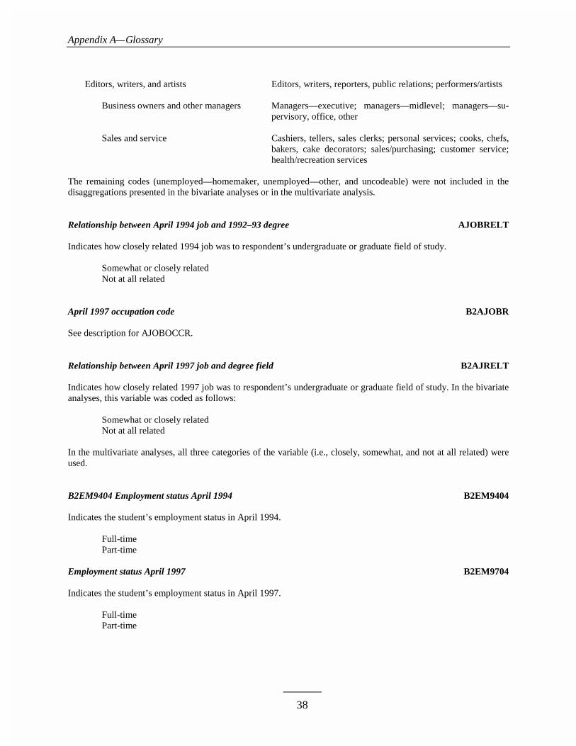
Appendix A—Glossary
38
Editors, writers, and artists Editors, writers, reporters, public relations; performers/artists
Business owners and other managers Managers—executive; managers—midlevel; managers—su-pervisory, office, other
Sales and service Cashiers, tellers, sales clerks; personal services; cooks, chefs,bakers, cake decorators; sales/purchasing; customer service;health/recreation services
The remaining codes (unemployed—homemaker, unemployed—other, and uncodeable) were not included in thedisaggregations presented in the bivariate analyses or in the multivariate analysis.
Relationship between April 1994 job and 1992–93 degree AJOBRELT
Indicates how closely related 1994 job was to respondent’s undergraduate or graduate field of study.
Somewhat or closely relatedNot at all related
April 1997 occupation code B2AJOBR
See description for AJOBOCCR.
Relationship between April 1997 job and degree field B2AJRELT
Indicates how closely related 1997 job was to respondent’s undergraduate or graduate field of study. In the bivariateanalyses, this variable was coded as follows:
Somewhat or closely relatedNot at all related
In the multivariate analyses, all three categories of the variable (i.e., closely, somewhat, and not at all related) wereused.
B2EM9404 Employment status April 1994 B2EM9404
Indicates the student’s employment status in April 1994.
Full-timePart-time
Employment status April 1997 B2EM9704
Indicates the student’s employment status in April 1997.
Full-time Part-time

Appendix A—Glossary
39
Undergraduate major recoded BAMAJOR
Identifies a respondent’s undergraduate major field of study. Majors were classified as follows:
Education Early childhood, elementary, secondary, special, physical, other
Engineering, mathematics, science Architecture, engineering (electrical, chemical, civil, mechani-cal, other), technology, mathematics, statistics, physical science,chemistry, earth science, physics, biological science (zoology,botany, biochemistry, other), biophysics, interdisciplinary (envi-ronmental studies, biopsychology, integrated/general)
Other Computer programming, computer and information sciences,nursing, dental/medical tech, community/mental health, nurseassisting, general and other health, health/physical educa-tion/recreation (HPER), audiology, clinical health science,health/hospital administration, dietetics, journalism, communi-cations, communication technology, American civilization, areastudies, African American studies, ethnic studies, Spanish, for-eign languages (non-European, European), letters (Eng-lish/American literature, creative/technical writing, other),liberal studies, women’s studies, philosophy, religious studies,history, design, speech/drama, film arts, music, art history/finearts, other fine and performing arts, clinical pastoral care, pro-tective services, social work, public administration, psychology,anthropology/archaeology, economics, geography, sociology,political science, international relations, city planning, agricul-ture, agricultural science, natural resources, forestry, textiles,other home economics, vocational home economics, guidance,law (paralegal, pre-law, law), library/archival science, militaryscience, other interdisciplinary, leisure studies, basic/personalskills, industrial arts (construction, commercial art, precisionproduction), air transportation
Panel weight for NPSAS and B&B BNBPANEL
Panel weight for NPSAS, B&B93/94, and B&B93/97 response. This is the panel weight for B&B:93/97, which isB0 adjusted for nonresponse at any of the follow-up surveys. Panel respondents are those who responded to all threesurveys: NPSAS:93, B&B:93/94, and B&B:93/97. Therefore, the panel category is greater than 0 for only those per-sons who responded to all three surveys.
Appendix A—Glossary
40
Highest degree program enrolled after BA B2HENPRG
Identifies degree type for the highest degree enrolled after bachelor’s degree. The following groups were defined.
Any postsecondary enrollmentAssociate degreeBachelors degreePost-baccalaureate certificateMasters degreeMBAPost-masters certificateFirst professionalDoctoral degreeCertificate or licenseNon-degree program
Any graduate enrollmentPost-baccalaureate certificateMasters degreeMBAPost-masters certificateFirst professionalDoctoral degreeCertificate or licenseNon-degree program
Student’s gender GENDER
Respondent’s gender.
MaleFemale
Student’s cumulative grade point average GPA
Indicates respondent’s cumulative grade point average. This variable was coded as follows:
Less than 2.752.75 - 2.993.00 - 3.493.50 or higher
Appendix A—Glossary
41
Comparison of April 1994 and April 1997 occupations OCHANGE
Identifies whether respondents were in the same occupation in April 1997 as they had been in April 1994. Graduateswhose April 1994 occupation category exactly matched the April 1997 occupation category were defined as in the“same” occupation category at the two points in time. In addition, the following occupation category combinationswere defined as “same” occupation for the purposes of this variable because they are likely to represent movementswithin a career or occupation ladder:
Clerks—secretarial, Clerks—data entry, Clerks—otherMedical licensed professionals and medical service occupationsMedical licensed professionals and medical practice professionalsLegal support workers and legal professionalsClerks—sales and sales/purchasing workersClerks—sales and customer service workersBusiness/financial support service workers and financial services professionalsBusiness/financial support service workers and Managers—supervisory, office, and other administrativeResearch assistants/lab technicians and researchersResearch assistants/lab technicians (which includes engineering assistants) and engineering and architec-tural professionals/engineersComputer operators, computer programmers, and computer systems/related professional/technical workersComputer systems/related professional/technical workers, computer programmers, and engineering and ar-chitectural professionals/engineersRepair workers, craftsmen, skilled operatives, and transport operatives (other than pilots)
Graduates with all other combinations of occupation categories were defined as working in “different” occupationcategories at the two points in time.
College entrance examination scores SATACTQ2
Indicates respondent’s merged SAT and ACT score quartile. Responses were coded as follows:
Bottom quartileSecond quartileThird quartileTop quartile
Professional status of April 1994 job PROSTA94
Indicates the professional status of respondent’s April 1994 job. Responses were grouped in following ways:
No degree needed, not much career potentialNo degree needed, possible or definite career potentialDegree needed, not much career potentialDegree needed, possible or definite career potential

Appendix A—Glossary
42
Professional status of April 1997 job PROSTA97
Indicates the professional status of respondent’s April 1997 job. Responses were classified as follows:
No degree needed, not much career potentialNo degree needed, possible or definite career potentialDegree needed, not much career potentialDegree needed, possible or definite career potential
43
Appendix B Technical Notes and Methodology
The Baccalaureate and Beyond Longitudinal Study8
The data analyzed in this report came from the First and Second Follow-ups of the Bacca-
laureate and Beyond Longitudinal Study (B&B:93/94 and B&B:93/97), a study that tracks the
experiences of a cohort of college graduates who received baccalaureate degrees during the
1992–93 academic year and were first interviewed as part of the National Postsecondary Student
Aid Study (NPSAS:93). This group’s experiences in the areas of academic enrollments, degree
completions, employment, public service, and such other adult decisions as family formation
have been followed through 1997. The data derived from this survey provide critical information
about college graduates’ postsecondary education outcomes, including graduate and professional
program access, labor market experience, and rates of return on investment in education.
The B&B: 93/94 survey was the first follow-up interview of NPSAS:93 participants who
received their bachelor’s degrees between July 1992 and June 1993. Of approximately 12,500
NPSAS:93 respondents who were identified as potentially eligible for the first follow-up survey,
about 1,500 were determined to be ineligible. Approximately 10,100 eligible individuals com-
pleted the 1994 interview.
The B&B:93/97 survey is the second follow-up interview of the B&B cohort. The first
follow-up interview (B&B:93/94) collected information from respondents 1 year after they re-
ceived the bachelor’s degree; the second follow-up (B&B:93/97) collected data 4 years after they
received the bachelor’s degree. Data collection for B&B:93/97 took place between April and De-
cember 1997. About 11,200 individuals in the B&B cohort were determined eligible for follow-
up in 1997. For the second follow-up, about 10,100 interviews were completed, yielding a re-
sponse rate of 90 percent. Approximately 9,300 individuals (83 percent of the sample) responded
to all three rounds of the B&B study. Referred to as “the B&B panel sample,” these respondents
became the base sample of the analyses presented in this report.
The NPSAS:93 sample, while representative and statistically accurate, was not a simple
random sample. Instead, the survey sample was selected using a more complex three-step proce-
dure with stratified samples and differential probabilities of selection at each level. Postsecon- 8The text in this section is based on excerpts from the Baccalaureate and Beyond Longitudinal Study: 1993/97 MethodologyReport (NCES 1999–159) (Washington, DC: U.S. Department of Education, National Center for Education Statistics, 1999).
Appendix B—Technical Notes and Methodology
44
dary institutions were initially selected within geographic strata. Once institutions were organ-
ized by zip code and state, they were further stratified by control (i.e., public; private, not-for-
profit; or private, for-profit) and degree offering (less-than-2-year, 2- to 3-year, 4-year nondoc-
torate-granting, and 4-year doctorate-granting).9
For more information about the NPSAS:93 survey, refer to the Methodology Report for the
National Postsecondary Student Aid Study, 1992–93 (NCES 95–211, Washington, DC: U.S. De-
partment of Education, National Center for Education Statistics, 1995). For more information on
procedures for the Baccalaureate and Beyond First Follow-up Study (B&B:93/94), consult the
Baccalaureate and Beyond Longitudinal Study Methodology Report (NCES 96–149). For second
follow-up, consult NCES 1999–159.
Sample weights. B&B:93/97 final weights were calculated by making a nonresponse ad-
justment to the baseline B&B weight calculated for B&B:93/94. This baseline B&B weight is an
adjustment of the baseline NPSAS:93 weight to reflect final eligibility for B&B and to reflect the
total number of bachelor’s degrees awarded in 1992–93. All analyses in this report are weighted
to compensate for unequal probability of selection into the B&B sample and to adjust for nonre-
sponse. The B&B panel weight, based on respondents who participated in all three surveys, is
used in the report. A complete description of the weighting methodology is available in the
methodology reports cited above.
Accuracy of Estimates
The statistics in this report are estimates derived from a sample. Two broad categories of
error occur in such estimates: sampling and nonsampling errors. Sampling errors occur because
observations are made only on samples of students, not on entire populations. Surveys of popu-
lation universes are not subject to sampling errors. Estimates based on a sample will differ
somewhat from those that would have been obtained by a complete census of the relevant popu-
lation using the same survey instruments, instructions, and procedures. The standard error of a
statistic is a measure of the variation due to sampling; it indicates the precision of the statistic
obtained in a particular sample. In addition, the standard errors for two sample statistics can be
used to estimate the precision of the difference between the two statistics and to help determine
whether the difference based on the sample is likely to represent a population difference. Tables
B1a and B1b present standard errors for figures 2 and 4 of this report. Additional standard errors
9The NPSAS universe excludes institutions offering only correspondence courses, institutions enrolling only their own employ-ees, and U.S. service academies. For this B&B cohort, institutions were further stratified in NPSAS by the number of degrees ineducation they had awarded in the past.
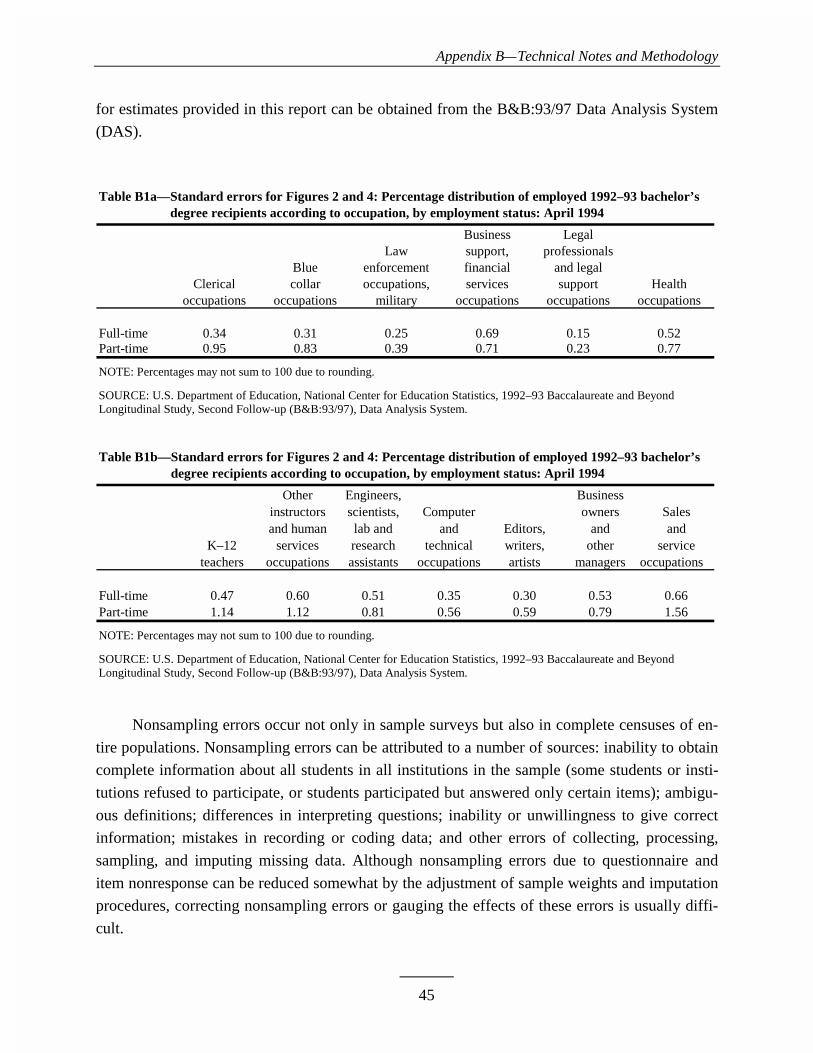
Appendix B—Technical Notes and Methodology
45
for estimates provided in this report can be obtained from the B&B:93/97 Data Analysis System
(DAS).
Table B1a—Standard errors for Figures 2 and 4: Percentage distribution of employed 1992–93 bachelor’s Table B1a—degree recipients according to occupation, by employment status: April 1994
Business Legal Law support, professionals Blue enforcement financial and legal Clerical collar occupations, services support Health
occupations occupations military occupations occupations occupations
Full-time 0.34 0.31 0.25 0.69 0.15 0.52Part-time 0.95 0.83 0.39 0.71 0.23 0.77
NOTE: Percentages may not sum to 100 due to rounding.
SOURCE: U.S. Department of Education, National Center for Education Statistics, 1992–93 Baccalaureate and BeyondLongitudinal Study, Second Follow-up (B&B:93/97), Data Analysis System.
Table B1b—Standard errors for Figures 2 and 4: Percentage distribution of employed 1992–93 bachelor’s Table B1b—degree recipients according to occupation, by employment status: April 1994
Other Engineers, Businessinstructors scientists, Computer owners Sales
and human lab and and Editors, and andK–12 services research technical writers, other service
teachers occupations assistants occupations artists managers occupations
Full-time 0.47 0.60 0.51 0.35 0.30 0.53 0.66Part-time 1.14 1.12 0.81 0.56 0.59 0.79 1.56
NOTE: Percentages may not sum to 100 due to rounding.
SOURCE: U.S. Department of Education, National Center for Education Statistics, 1992–93 Baccalaureate and BeyondLongitudinal Study, Second Follow-up (B&B:93/97), Data Analysis System.
Nonsampling errors occur not only in sample surveys but also in complete censuses of en-
tire populations. Nonsampling errors can be attributed to a number of sources: inability to obtain
complete information about all students in all institutions in the sample (some students or insti-
tutions refused to participate, or students participated but answered only certain items); ambigu-
ous definitions; differences in interpreting questions; inability or unwillingness to give correct
information; mistakes in recording or coding data; and other errors of collecting, processing,
sampling, and imputing missing data. Although nonsampling errors due to questionnaire and
item nonresponse can be reduced somewhat by the adjustment of sample weights and imputation
procedures, correcting nonsampling errors or gauging the effects of these errors is usually diffi-
cult.

Appendix B—Technical Notes and Methodology
46
Data Analysis System
The estimates presented in this report were produced using the B&B:93/97 Data Analysis
System (DAS). The DAS software makes it possible for users to specify and generate their own
tables from the B&B:93/97 data. With the DAS, users can replicate or expand upon the tables
presented in this report. In addition to the table estimates, the DAS calculates proper standard
errors10 and weighted sample sizes for these estimates. For example, table B1 contains estimated
standard errors that correspond to the estimates presented in Figures 2 and 4 and that were gener-
ated by the B&B:93/97 DAS. If the number of valid cases is too small to produce a reliable esti-
mate (fewer than 30 cases), the DAS prints the message “low N” instead of the estimate.
In addition to tables, the DAS will also produce a correlation matrix of selected variables to
be used for linear regression models. Included in the output with the correlation matrix are the
design effects (DEFTs) for each variable in the matrix. Since statistical procedures generally
compute standard errors based on an assumption of simple random sampling, the standard errors
must be adjusted with the design effects to take into account B&B’s complex sample design.
(See discussion under “Statistical Procedures” below for the adjustment procedure.)
For more information about the B&B:93/97 and other Data Analysis Systems, consult the
NCES DAS website (nces.ed.gov/das) or contact:
Aurora D’AmicoNational Center for Education Statistics1990 K Street, NWRoom 8115Washington, DC 20006(202) 502-7334Internet address: Aurora_D’[email protected]
Statistical Procedures
Differences Between Means
The descriptive comparisons were tested in this report using Student’s t statistic. Differ-
ences between estimates are tested against the probability of a Type I error,11 or significance
level. The significance levels were determined by calculating the Student’s t values for the dif-
10The B&B sample is not a simple random sample, and therefore simple random sample techniques for estimating sampling errorcannot be applied to these data. The DAS takes into account the complexity of the sampling procedures and calculates standarderrors appropriate for such samples. The method for computing sampling errors used by the DAS involves approximating theestimator by the linear terms of a Taylor series expansion. The procedure is typically referred to as the Taylor series method.11A Type I error occurs when one concludes that a difference observed in a sample reflects a true difference in the populationfrom which the sample was drawn, when no such difference is present.

Appendix B—Technical Notes and Methodology
47
ferences between each pair of means or proportions and comparing these with published tables of
significance levels for two-tailed hypothesis testing.
Student’s t values may be computed to test the difference between estimates with the fol-
lowing formula:
22
21
21
sese
EEt
+
−= (1)
where E1 and E2 are the estimates to be compared and se1 and se2 are their corresponding stan-
dard errors. This formula is valid only for independent estimates. When estimates are not inde-
pendent, a covariance term must be added to the formula:
E - E
se + se - 2(r)se se1 2
12
22
1 2
(2)
where r is the correlation between the two estimates.12 This formula is used when comparing two
percentages from a distribution that adds to 100. If the comparison is between the mean of a sub-
group and the mean of the total group, which is the primary comparison in this report, the fol-
lowing formula is used:
2sub
2tot
2sub
totsub
se p2sese
EE
−+
−(3)
where p is the proportion of the total group contained in the subgroup.13 The estimates, standarderrors, and correlations can all be obtained from the DAS.
There are hazards in reporting statistical tests for each comparison. First, comparisons
based on large t statistics may appear to merit special attention. This can be misleading since the
magnitude of the t statistic is related not only to the observed differences in means or percentages
but also to the number of students in the specific categories used for comparison. Hence, a small
difference compared across a large number of students would produce a large t statistic.
A second hazard in reporting statistical tests for each comparison occurs when making
multiple comparisons among categories of an independent variable. For example, when making
12U.S. Department of Education, National Center for Education Statistics, A Note from the Chief Statistician, no. 2, 1993.13Ibid.
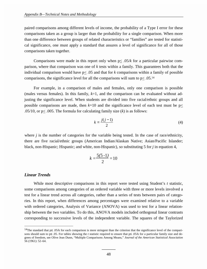
Appendix B—Technical Notes and Methodology
48
paired comparisons among different levels of income, the probability of a Type I error for these
comparisons taken as a group is larger than the probability for a single comparison. When more
than one difference between groups of related characteristics or “families” are tested for statisti-
cal significance, one must apply a standard that assures a level of significance for all of those
comparisons taken together.
Comparisons were made in this report only when p< .05/k for a particular pairwise com-
parison, where that comparison was one of k tests within a family. This guarantees both that the
individual comparison would have p< .05 and that for k comparisons within a family of possible
comparisons, the significance level for all the comparisons will sum to p< .05.14
For example, in a comparison of males and females, only one comparison is possible
(males versus females). In this family, k=1, and the comparison can be evaluated without ad-
justing the significance level. When students are divided into five racial/ethnic groups and all
possible comparisons are made, then k=10 and the significance level of each test must be p<
.05/10, or p< .005. The formula for calculating family size (k) is as follows:
kj j= −( )1
2(4)
where j is the number of categories for the variable being tested. In the case of race/ethnicity,
there are five racial/ethnic groups (American Indian/Alaskan Native; Asian/Pacific Islander;
black, non-Hispanic; Hispanic; and white, non-Hispanic), so substituting 5 for j in equation 4,
k =5(5 -1)
2=10
Linear Trends
While most descriptive comparisons in this report were tested using Student’s t statistic,
some comparisons among categories of an ordered variable with three or more levels involved a
test for a linear trend across all categories, rather than a series of tests between pairs of catego-
ries. In this report, when differences among percentages were examined relative to a variable
with ordered categories, Analysis of Variance (ANOVA) was used to test for a linear relation-
ship between the two variables. To do this, ANOVA models included orthogonal linear contrasts
corresponding to successive levels of the independent variable. The squares of the Taylorized
14The standard that p≤ .05/k for each comparison is more stringent than the criterion that the significance level of the compari-sons should sum to p≤ .05. For tables showing the t statistic required to ensure that p≤ .05/k for a particular family size and de-grees of freedom, see Olive Jean Dunn, “Multiple Comparisons Among Means,” Journal of the American Statistical Association56 (1961): 52–64.

Appendix B—Technical Notes and Methodology
49
standard errors (that is, standard errors that were calculated by the Taylor series method), the
variance between the means, and the unweighted sample sizes were used to partition total sum of
squares into within- and between-group sums of squares. These were used to create mean
squares for the within- and between-group variance components and their corresponding F sta-
tistics, which were then compared with published values of F for a significance level of .05.15
Significant values of both the overall F and the F associated with the linear contrast term were
required as evidence of a linear relationship between the two variables. Means and Taylorized
standard errors were calculated by the DAS. Unweighted sample sizes are not available from the
DAS and were provided by NCES.
Adjustment of Means to Control for Background Variation
Tabular results are limited by sample size when attempting to control for additional factors
that may account for the variation observed between two variables. For example, when examin-
ing percentages of graduates who worked in the same occupations in April 1994 and April 1997,
it is impossible to know to what extent the observed variation is due to the April 1994 occupation
and to what extent it is due to differences in graduates’ perceptions of their occupations’ rela-
tionships to their fields of study or professional status. However, if a nested table were produced
showing the percentage who worked in the same occupation within occupations within relation-
ship to degree fields within perceptions of professional status, the cell sizes would be too small
to identify the patterns. When the sample size becomes too small to support controls for covaria-
tion, one must use other methods to take such covariation into account.
To overcome this difficulty, multiple linear regression was used to obtain means that were
adjusted for covariation among a list of control variables.16 Adjusted means for subgroups were
obtained by regressing the dependent variable on a set of descriptive variables such as gender,
age, employment status, occupation, relationship of occupation to degree fields, perceived pro-
fessional status of occupation, and so on. Substituting ones or zeros for the subgroup characteris-
tic(s) of interest and the mean proportions for the other variables results in an estimate of the
adjusted proportion for the specified subgroup, holding the other variables in the equation con-
stant. For example, consider a hypothetical case in which two variables, age and gender, are used
to describe an outcome, Y (such as percentage of graduates working the same occupation in both
April 1994 and April 1997). The variables age and gender are recoded into a dummy variable
representing age, A, and a dummy variable representing gender, G:
15More information about ANOVA and significance testing using the F statistic can be found in any standard textbook on statis-tical methods in the social and behavioral sciences.16For more information about weighted least squares regression, see Michael S. Lewis-Beck, Applied Regression: An Introduc-tion, Vol. 22 (Beverly Hills, CA: Sage Publications, Inc., 1980); William D. Berry and Stanley Feldman, Multiple Regression inPractice, Vol. 50 (Beverly Hills, CA: Sage Publications, Inc., 1987).
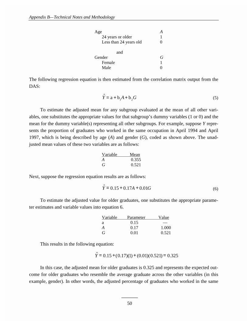
Appendix B—Technical Notes and Methodology
50
Age A24 years or older 1Less than 24 years old 0
andGender G
Female 1Male 0
The following regression equation is then estimated from the correlation matrix output from the
DAS:
ˆ Y = a + b1A + b2G (5)
To estimate the adjusted mean for any subgroup evaluated at the mean of all other vari-
ables, one substitutes the appropriate values for that subgroup’s dummy variables (1 or 0) and the
mean for the dummy variable(s) representing all other subgroups. For example, suppose Y repre-
sents the proportion of graduates who worked in the same occupation in April 1994 and April
1997, which is being described by age (A) and gender (G), coded as shown above. The unad-
justed mean values of these two variables are as follows:
Variable MeanA 0.355G 0.521
Next, suppose the regression equation results are as follows:
ˆ Y = 0.15 + 0.17A + 0.01G (6)
To estimate the adjusted value for older graduates, one substitutes the appropriate parame-
ter estimates and variable values into equation 6.
Variable Parameter Valuea 0.15 —A 0.17 1.000G 0.01 0.521
This results in the following equation:
ˆ Y = 0.15 +(0.17)(1) + (0.01)(0.521) = 0.325
In this case, the adjusted mean for older graduates is 0.325 and represents the expected out-
come for older graduates who resemble the average graduate across the other variables (in this
example, gender). In other words, the adjusted percentage of graduates who worked in the same

Appendix B—Technical Notes and Methodology
51
occupation at both points in time, controlling for age and gender, is 32.5 percent (0.325 x 100 for
conversion to a percentage).
It is relatively straightforward to produce a multivariate model using the DAS, since one of
the DAS output options is a correlation matrix, computed using pairwise missing values. In re-
gression analysis, there are several common approaches to the problem of missing data. The two
simplest are pairwise deletion of missing data and listwise deletion of missing data. In pairwise
deletion, each correlation is calculated using all of the cases for the two relevant variables. For
example, suppose you have a regression analysis that uses variables X1, X2, and X3. The regres-
sion is based on the correlation matrix between X1, X2, and X3. In pairwise deletion the correla-
tion between X1 and X2 is based on the nonmissing cases for X1 and X2. Cases missing on
either X1 or X2 would be excluded from the calculation of the correlation. In listwise deletion
the correlation between X1 and X2 would be based on the nonmissing values for X1, X2, and
X3. That is, all of the cases with missing data on any of the three variables would be excluded
from the analysis.17
The correlation matrix can be used by most statistical software packages as the input data
for least squares regression. That is the approach used for this report, with an additional adjust-
ment to incorporate the complex sample design into the statistical significance tests of the pa-
rameter estimates (described below). For tabular presentation, parameter estimates and standard
errors were multiplied by 100 to match the scale used for reporting unadjusted and adjusted per-
centages.
Most statistical software packages assume simple random sampling when computing stan-
dard errors of parameter estimates. Because of the complex sampling design used for the NPSAS
survey, this assumption is incorrect. A better approximation of their standard errors is to multiply
each standard error by the design effect associated with the dependent variable (DEFT),18 where
the DEFT is the ratio of the true standard error to the standard error computed under the assump-
tion of simple random sampling. It is calculated by the DAS and produced with the correlation
matrix.
17Although the DAS simplifies the process of making regression models, it also limits the range of models. Analysts who wish touse an approach other than pairwise treatment of missing values or to estimate probit/logit models (which are the most appropri-ate for models with categorical dependent variables) can apply for a restricted data license from NCES. See John H. Aldrich andForrest D. Nelson, Linear Probability, Logit and Probit Models (Quantitative Applications in Social Sciences, Vol. 45) (BeverlyHills, CA: Sage, 1984).18The adjustment procedure and its limitations are described in C.J. Skinner, D. Holt, and T.M.F. Smith, eds., Analysis of Com-plex Surveys (New York: John Wiley & Sons, 1989).