MULTISCALE DYNAMIC MONTE CARLO / CONTINUUM MODELING OF DRYING AND

University of KentuckyUKnowledge

University of Kentucky Doctoral Dissertations Graduate School

2008

MULTISCALE DYNAMIC MONTE CARLO /CONTINUUM MODELING OF DRYINGAND CURING IN SOL-GEL SILICA FILMSXin LiUniversity of Kentucky, [email protected]

Click here to let us know how access to this document benefits you.

This Dissertation is brought to you for free and open access by the Graduate School at UKnowledge. It has been accepted for inclusion in University ofKentucky Doctoral Dissertations by an authorized administrator of UKnowledge. For more information, please contact [email protected].

Recommended CitationLi, Xin, "MULTISCALE DYNAMIC MONTE CARLO / CONTINUUM MODELING OF DRYING AND CURING IN SOL-GEL SILICA FILMS" (2008). University of Kentucky Doctoral Dissertations. 662.https://uknowledge.uky.edu/gradschool_diss/662

http://uknowledge.uky.edu/

http://uknowledge.uky.edu/

https://uknowledge.uky.edu

https://uknowledge.uky.edu/gradschool_diss

https://uknowledge.uky.edu/gradschool

https://uky.az1.qualtrics.com/jfe/form/SV_9mq8fx2GnONRfz7

mailto:[email protected]

ABSTRACT OF DISSERTATION

Xin Li

The Graduate School

University of Kentucky

2008

MULTISCALE DYNAMIC MONTE CARLO / CONTINUUM MODELING OF DRYING AND CURING IN SOL-GEL SILICA FILMS


A dissertation submitted in partial fulfillment of the

requirements for the degree of Doctor of Philosophy in the College of Engineering

at the University of Kentucky

By Xin Li

Lexington, Kentucky

Director: Dr. Stephen E. Rankin, Associate Professor of Chemical Engineering

Lexington, Kentucky

2008

Copyright © Xin Li 2008


Modeling the competition between drying and curing processes in polymerizing films is of great importance to many existing and developing materials synthesis processes. These processes involve multiple length and time scales ranging from molecular to macroscopic, and are challenging to fully model in situations where the polymerization is non-ideal, such as sol-gel silica thin film formation. A comprehensive model of sol-gel silica film formation should link macroscopic flow and drying (controlled by process parameters) to film microstructure (which dictates the properties of the films). This dissertation describes a multiscale model in which dynamic Monte Carlo (DMC) polymerization simulations are coupled to a continuum model of drying. Unlike statistical methods, DMC simulations track the entire molecular structure distribution to allow the calculation not only of molecular weight but also of cycle ranks and topological indices related to molecular size and shape. The entire DMC simulation (containing 106 monomers) is treated as a particle of sol whose position and composition are tracked in the continuum mass transport model of drying. The validity of the multiscale model is verified by the good agreement of the conversion evolution of DMC and continuum simulations for ideal polycondensation and first shell substitution effect (FSSE) cases. Because our model allows cyclic and cage-like siloxanes to form, it is better able to predict the silica gelation conversion than other reported kinetic models. By studying the competition between molecular growth and cyclization, and the competition between mass transfer (drying) and reaction (gelation) on the drying process of the sol-gel silica film, we observe that cyclization delays gelation, shrinks the molecular size, increases the likelihood of skin formation, and leads to a molecular structure gradient inside the film. We also find that compared with a model with only 3-membered rings, the molecular structure is more complicated and the structure gradients in the films are larger with 4-membered rings. We expect that our simulation will allow better prediction of the formation of structure gradients in sol-gel derived ceramics and other nonideal multifunctional polycondensation products, and that this will help in developing


procedures to reduce coating defects. KEYWORDS: Multiscale modeling, sol-gel silica films, dynamic Monte Carlo, polycondensation, cyclization

Xin Li o

o


By

Xin Li

Dr. Stephen E. Rankin o Director of Dissertation

Dr. Barbara Knutson t Director of Graduate Studies

o

Date

RULES FOR THE USE OF DISSERTATIONS

Unpublished dissertations submitted for the Doctor's degree and deposited in the University of Kentucky Library are as a rule open for inspection, but are to be used only with due regard to the rights of the authors. Bibliographical references may be noted, but quotations or summaries of parts may be published only with the permission of the author, and with the usual scholarly acknowledgements. Extensive copying or publication of the dissertation in whole or in part also requires the consent of the Dean of the Graduate School of the University of Kentucky. A library that borrows this dissertation for use by its patrons is expected to secure the signature of each user. Name Date

DISSERTATION

Xin Li

The Graduate School

University of Kentucky

2008


DISSERTATION

A dissertation submitted in partial fulfillment of the requirements for the degree of Doctor of Philosophy in the

College of Engineering at the University of Kentucky

By Xin Li

Lexington, Kentucky

Director: Dr. Stephen E. Rankin, Associate Professor of Chemical Engineering

Lexington, Kentucky

2008

Copyright © Xin Li 2008

iii

ACKNOWLEDGEMENTS

First, I would like to sincerely express my thanks to my advisor, Dr. Stephen E. Rankin,

for his continuous support, encouragement, and patience, during my doctoral research.

I am also extremely grateful to my dissertation committee members, Drs. Douglass S.

Kalika, M. Pinar Mengüç, Zhongwei Shen, and Tate T.H. Tsang, for their precious

suggestions and time.

Finally, I am forever indebted to my husband, Fan, and my parents, Bingrong Li and

Fengming Chen for their love, understanding, and support throughout these years.

This work was funded by Department of Energy under Grant DE-FG02-03ER46033.

iv

TABLE OF CONTENTS

Acknowledgements............................................................................................................iii

List of Tables....................................................................................................................viii

List of Figures.....................................................................................................................ix

List of Files........................................................................................................................xii

Chapter 1 Sol-Gel Silica Chemistry for Multiscale Modeling of Drying and Curing ........ 1

1.1 Motivation................................................................................................................. 1

1.2 Sol-gel chemistry ...................................................................................................... 2

1.2.1 Hydrolysis Pseudoequilibrium........................................................................... 3

1.2.2 First Shell Substitution Effect (FSSE) ............................................................... 4

1.2.3 Bimolecular Site-level Condensation ................................................................ 4

1.2.4 Cyclization ......................................................................................................... 6

1.3 Dissertation Outline .................................................................................................. 7

Chapter 2 Introduction to Molecular and Continuum Simulation Methods ....................... 9

2.1 Molecular Modeling Technique – Dynamic Monte Carlo (DMC) Method ............. 9

2.1.1 Introduction........................................................................................................ 9

2.1.2 DMC Algorithm............................................................................................... 11

2.1.2.1 Data Structures.......................................................................................... 12

2.1.2.2 Monte Carlo Reaction Selection ............................................................... 14

2.1.2.3 Flow Sheet ................................................................................................ 14

2.1.3 Random Branching Theory (RBT) .................................................................. 17

2.1.4 Results and Discussion .................................................................................... 18

2.2 Continuum Modeling Method – Finite Difference Method (FDM) ....................... 18

2.2.1 Introduction...................................................................................................... 18

2.2.2 FDM Algorithm ............................................................................................... 22

2.2.2.1 Discretization (grid) .................................................................................. 24

2.2.2.2 Explicit Scheme ........................................................................................ 24

2.3 Summary ................................................................................................................. 26

Chapter 3 Multiscale Modeling of Ideal Polycondensation and Polycondensation with

First Shell Substitution Effect (FSSE) in Drying Thin Films ........................................... 27

v

3.1 Introduction............................................................................................................. 27

3.2 DMC Model ............................................................................................................ 29

3.3 Continuum Drying Model....................................................................................... 31

3.3.1 Model Assumptions and Description............................................................... 31

3.3.2 Governing Equations ....................................................................................... 33

3.3.3 Dimensionless Variables and Simulation Procedure ....................................... 35

3.3.4 Tracking the Sol Particle.................................................................................. 35

3.4 Results and Discussion ........................................................................................... 37

3.4.1 Solvent Concentration Profile.......................................................................... 37

3.4.2 Conversion and Site Distribution..................................................................... 40

3.4.3 Three Types of Drying and Gelation Phenomena............................................ 40

3.4.4 Gelation Regime Map...................................................................................... 44

3.4.5 Relationship between Gel Time and Initial Particle Position .......................... 50

3.5 Summary ................................................................................................................. 53

Chapter 4 Multiscale Modeling with Unlimited 3-membered Ring Cyclization.............. 54

4.1 Introduction............................................................................................................. 54

4.2 DMC Model ............................................................................................................ 56

4.2.1 Bimolecular Condensation............................................................................... 56

4.2.2 Three-membered Ring Cyclization.................................................................. 57

4.2.3 Wiener Index.................................................................................................... 59

4.2.4 Cycle Rank....................................................................................................... 63

4.2.5 Ring Involvement............................................................................................. 66

4.2.6 DMC Algorithm............................................................................................... 66


4.3.1 Model Description ........................................................................................... 67

4.3.2 Governing Equations ....................................................................................... 69


4.3.4 Parameters........................................................................................................ 70

4.4 Results and Discussion ........................................................................................... 71

4.4.1 Conversion at Gelation .................................................................................... 71

4.4.2 Wiener Index.................................................................................................... 73

vi

4.4.3 Cycle Rank....................................................................................................... 75

4.4.4 Ring Involvement............................................................................................. 75

4.4.5 Gelation Regime Map...................................................................................... 75

4.4.6 Structure Gradient Map.................................................................................... 83

4.4.7 The Effect of Solvent Vapor Pressure ............................................................. 86

4.5 Summary ................................................................................................................. 89

Chapter 5 Multiscale Modeling with Unlimited 4-membered Ring Cyclization.............. 91

5.1 Introduction............................................................................................................. 91

5.2 DMC Model ............................................................................................................ 92

5.2.1 Bimolecular Condensation............................................................................... 92

5.2.2 Four-membered Ring Cyclization.................................................................... 93

5.2.3 DMC Algorithm............................................................................................... 94


5.3.1 Model description ............................................................................................ 98

5.3.2 Governing equations ........................................................................................ 98


5.4 Results and discussion .......................................................................................... 100

5.4.1 Conversion at Gelation .................................................................................. 100

5.4.2 Wiener Index.................................................................................................. 105

5.4.3 Cycle Rank..................................................................................................... 105

5.4.4 Ring Involvement........................................................................................... 111

5.4.5 Gelation Regime Map.................................................................................... 111

5.4.6 Structure Gradient Map.................................................................................. 119

5.5 Summary ............................................................................................................... 124

Chapter 6 Conclusions .................................................................................................... 127

Appendix A. Calculation of Number- and Weight-average Parameters......................... 131

A.1 Definition ............................................................................................................. 131

A.1.1 Degree of Polymerization ............................................................................. 131

A.1.2 Cycle Rank.................................................................................................... 131

A.1.3 Wiener Index................................................................................................. 131

A.2 Bimolecular Condensation Reactions .................................................................. 132

vii

A.2.1 Degree of Polymerization ............................................................................. 132

A.2.2 Cycle Rank.................................................................................................... 132

A.2.3 Wiener Index................................................................................................. 133

A.3 Cyclization Reactions .......................................................................................... 133

A.3.1 Cycle Rank.................................................................................................... 133

A.3.2 Wiener Index................................................................................................. 134

Appendix B. Nomenclature ............................................................................................ 135

References....................................................................................................................... 137

Vita.................................................................................................................................. 143

viii

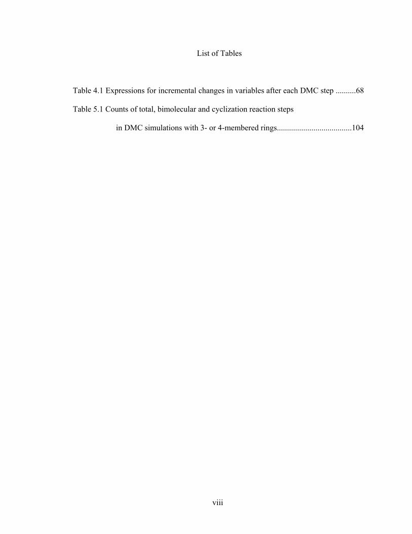
List of Tables

Table 4.1 Expressions for incremental changes in variables after each DMC step ..........68

Table 5.1 Counts of total, bimolecular and cyclization reaction steps

in DMC simulations with 3- or 4-membered rings.....................................104

ix

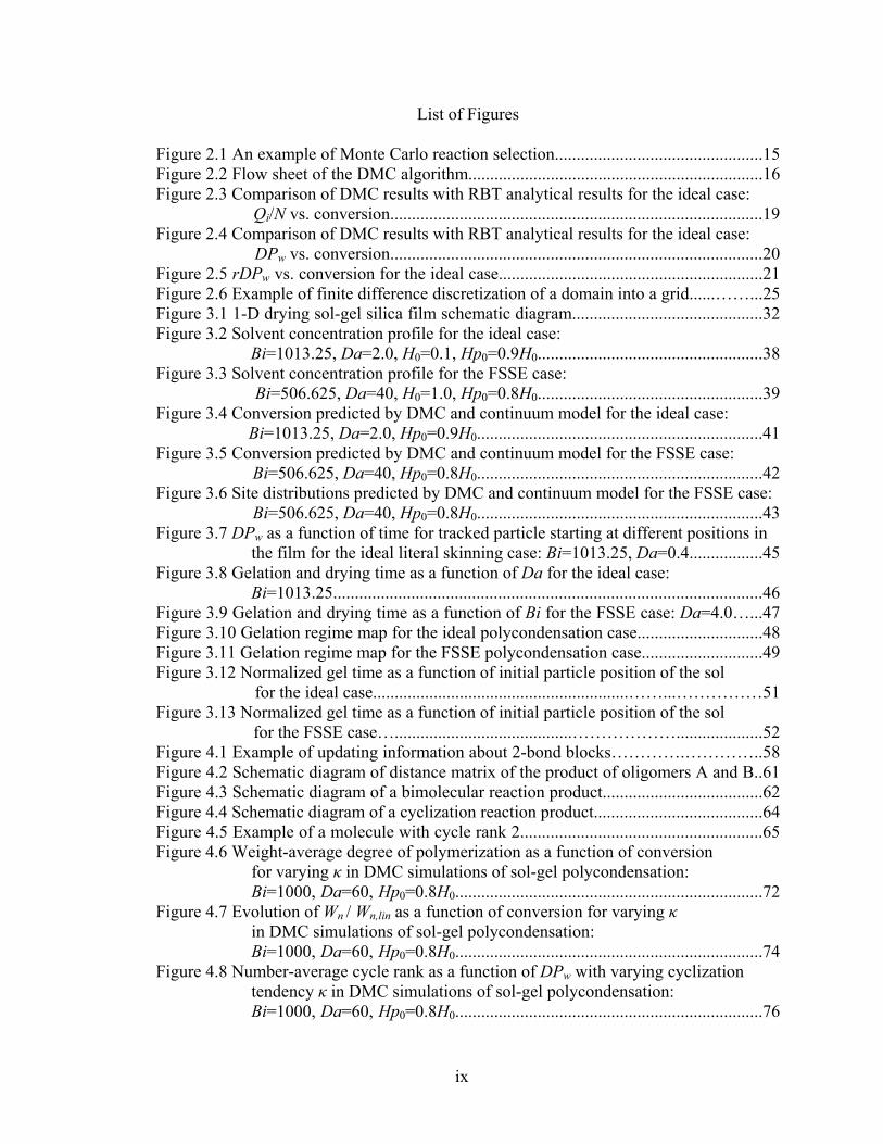
List of Figures

Figure 2.1 An example of Monte Carlo reaction selection................................................15 Figure 2.2 Flow sheet of the DMC algorithm....................................................................16 Figure 2.3 Comparison of DMC results with RBT analytical results for the ideal case: Qi/N vs. conversion......................................................................................19 Figure 2.4 Comparison of DMC results with RBT analytical results for the ideal case: DPw vs. conversion......................................................................................20 Figure 2.5 rDPw vs. conversion for the ideal case.............................................................21 Figure 2.6 Example of finite difference discretization of a domain into a grid......……...25 Figure 3.1 1-D drying sol-gel silica film schematic diagram............................................32 Figure 3.2 Solvent concentration profile for the ideal case: Bi=1013.25, Da=2.0, H0=0.1, Hp0=0.9H0....................................................38 Figure 3.3 Solvent concentration profile for the FSSE case:

Bi=506.625, Da=40, H0=1.0, Hp0=0.8H0....................................................39 Figure 3.4 Conversion predicted by DMC and continuum model for the ideal case:

Bi=1013.25, Da=2.0, Hp0=0.9H0..................................................................41 Figure 3.5 Conversion predicted by DMC and continuum model for the FSSE case: Bi=506.625, Da=40, Hp0=0.8H0..................................................................42 Figure 3.6 Site distributions predicted by DMC and continuum model for the FSSE case: Bi=506.625, Da=40, Hp0=0.8H0..................................................................43 Figure 3.7 DPw as a function of time for tracked particle starting at different positions in the film for the ideal literal skinning case: Bi=1013.25, Da=0.4.................45 Figure 3.8 Gelation and drying time as a function of Da for the ideal case: Bi=1013.25...................................................................................................46 Figure 3.9 Gelation and drying time as a function of Bi for the FSSE case: Da=4.0…...47 Figure 3.10 Gelation regime map for the ideal polycondensation case.............................48 Figure 3.11 Gelation regime map for the FSSE polycondensation case............................49 Figure 3.12 Normalized gel time as a function of initial particle position of the sol for the ideal case...........................................................……...……………51

Figure 3.13 Normalized gel time as a function of initial particle position of the sol for the FSSE case….........................................………………....................52 Figure 4.1 Example of updating information about 2-bond blocks………….…………..58 Figure 4.2 Schematic diagram of distance matrix of the product of oligomers A and B..61 Figure 4.3 Schematic diagram of a bimolecular reaction product.....................................62 Figure 4.4 Schematic diagram of a cyclization reaction product.......................................64 Figure 4.5 Example of a molecule with cycle rank 2........................................................65 Figure 4.6 Weight-average degree of polymerization as a function of conversion for varying κ in DMC simulations of sol-gel polycondensation: Bi=1000, Da=60, Hp0=0.8H0.......................................................................72 Figure 4.7 Evolution of Wn / Wn,lin as a function of conversion for varying κ in DMC simulations of sol-gel polycondensation: Bi=1000, Da=60, Hp0=0.8H0.......................................................................74 Figure 4.8 Number-average cycle rank as a function of DPw with varying cyclization tendency κ in DMC simulations of sol-gel polycondensation: Bi=1000, Da=60, Hp0=0.8H0.......................................................................76

x

Figure 4.9 Ring involvement as a function of conversion with varying cyclization tendency κ in DMC simulations of sol-gel polycondensation: Bi=1000, Da=60, Hp0=0.8H0..............................................……………….77 Figure 4.10 Gel conversion difference between the film surface and base with respect to κ in DMC simulations of sol-gel polycondensation: Bi=1000, Da=60...79 Figure 4.11 Gelation regime map with unlimited cyclization (3-membered ring) with κ=5 in drying sol-gel silica films.........................................................80 Figure 4.12 Number-average cycle rank as a function of time with different initial particle positions for cyclization literal skinning case: Bi=1000, Da=60, κ=5..................................................................................81 Figure 4.13 Ring involvement at the gel point as a function of initial particle positions for cyclization literal skinning case: Bi=1000, Da=60, κ=5..................................................................................82 Figure 4.14 Structure gradient map for cyclization case with κ=5....................................84 Figure 4.15 Example of contour plot of number-average cycle rank as functions of position and time calculated with Bi=800, Da=80, and κ=5........................85 Figure 4.16 Gelation regime map with unlimited cyclization (3-membered ring) for κ=5 with PE............................................................................................87 Figure 4.17 Structure gradient map for cyclization case for κ=5 with PE.........................88 Figure 5.1 Schematic diagram of the product of a cyclization reaction producing a 4-membered ring......................................................................95 Figure 5.2 Schematic showing how information about 3-bond blocks is updated due to an intramoleculer reaction.................................................................97 Figure 5.3 Weight-average degree of polymerization from DMC model with unlimited 4-membered rings as a function of conversion for varying κ: Bi=1000, Da=60, Hp0=0.8H0.....................................................................101 Figure 5.4 Gel conversion as a function of cyclization tendency κ with Bi=1000, Da=60, and Hp0=0.8H0..............................................................102 Figure 5.5 Evolution of Wn / Wn,lin as a function of conversion for varying κ in DMC simulations with 4-membered rings: Bi=1000, Da=60, Hp0=0.8H0.....................................................................106 Figure 5.5’ Evolution of Wn / Wn,lin as a function of conversion for varying κ in DMC simulations with 3-membered rings: Bi=1000, Da=60, Hp0=0.8H0.....................................................................107 Figure 5.6 Number-average cycle rank as a function of DPw with varying cyclization tendency κ for a DMC model with 4-membered rings: Bi=1000, Da=60, Hp0=0.8H0.....................................................................108 Figure 5.6’ Number-average cycle rank as a function of DPw with varying cyclization tendency κ for a DMC model with 3-membered rings: Bi=1000, Da=60, Hp0=0.8H0.....................................................................109 Figure 5.7 Ring involvement as a function of conversion with varying cyclization tendency κ for DMC simulations with 4-membered rings: Bi=1000, Da=60, Hp0=0.8H0.....................................................................112 Figure 5.7’ Ring involvement as a function of conversion with varying cyclization tendency κ for DMC simulations with 3-membered rings: Bi=1000, Da=60, Hp0=0.8H0.....................................................................113

xi

Figure 5.8 Gelation regime map with unlimited 4-membered ring cyclization calculated with κ=5....................................................................................115 Figure 5.8’ Gelation regime map with unlimited 3-membered ring cyclization calculated with κ=5....................................................................................116 Figure 5.9 Number-average cycle rank as a function of time with different initial particle positions for 4-membered ring cyclization: Bi=1000, Da=60, κ=5................................................................................117 Figure 5.9’ Number-average cycle rank as a function of time with different initial particle positions for 3-membered ring cyclization: Bi=1000, Da=60, κ=5................................................................................118 Figure 5.10 Ring involvement at the gel point as a function of initial particle positions for 4-membered ring cyclization literal skinning case: Bi=1000, Da=60, κ=5................................................................................120 Figure 5.10’ Ring involvement at the gel point as a function of initial particle positions for 3-membered ring cyclization literal skinning case: Bi=1000, Da=60, κ=5................................................................................121 Figure 5.11 Structure gradient map for the 4-membered ring cyclization case with κ=5.....................................................................................................122 Figure 5.11’ Structure gradient map for the 3-membered ring cyclization case with κ=5.....................................................................................................123

xii

List of Files

Dissertation_XL.pdf...................................................................................................1.3MB

1

Chapter 1

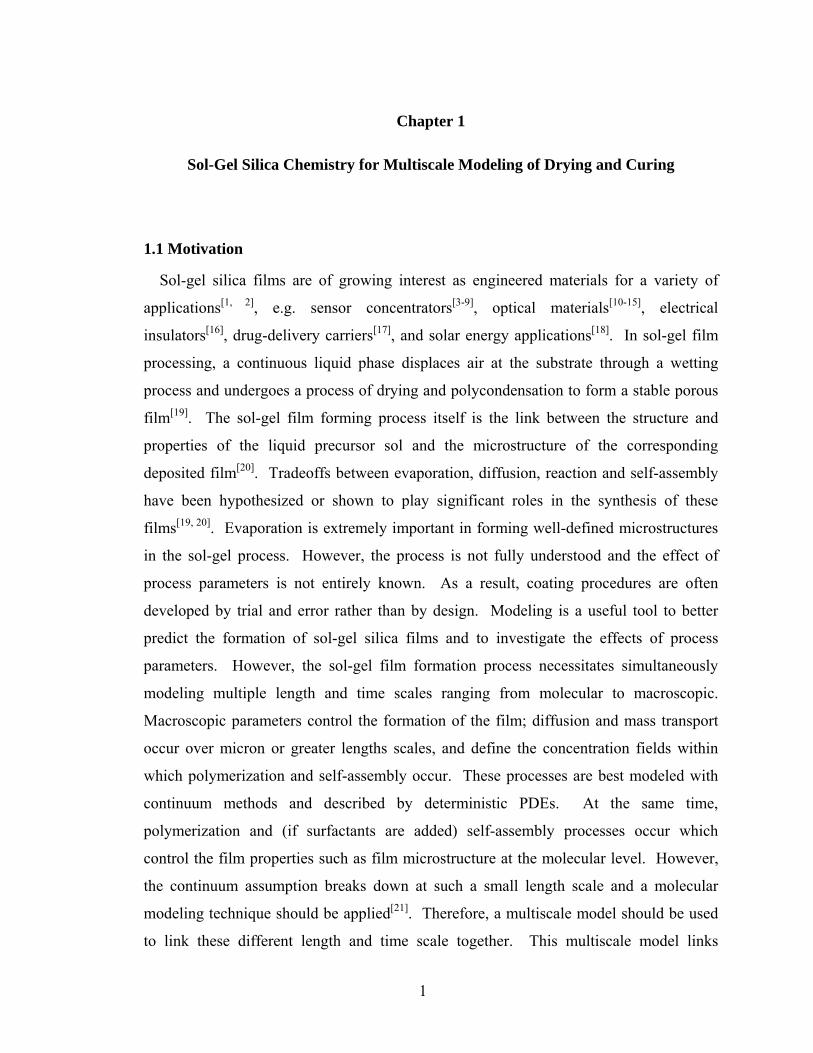
Sol-Gel Silica Chemistry for Multiscale Modeling of Drying and Curing

1.1 Motivation

Sol-gel silica films are of growing interest as engineered materials for a variety of

applications[1, 2], e.g. sensor concentrators[3-9], optical materials[10-15], electrical

insulators[16], drug-delivery carriers[17], and solar energy applications[18]. In sol-gel film

processing, a continuous liquid phase displaces air at the substrate through a wetting

process and undergoes a process of drying and polycondensation to form a stable porous

film[19]. The sol-gel film forming process itself is the link between the structure and

properties of the liquid precursor sol and the microstructure of the corresponding

deposited film[20]. Tradeoffs between evaporation, diffusion, reaction and self-assembly

have been hypothesized or shown to play significant roles in the synthesis of these

films[19, 20]. Evaporation is extremely important in forming well-defined microstructures

in the sol-gel process. However, the process is not fully understood and the effect of

process parameters is not entirely known. As a result, coating procedures are often

developed by trial and error rather than by design. Modeling is a useful tool to better

predict the formation of sol-gel silica films and to investigate the effects of process

parameters. However, the sol-gel film formation process necessitates simultaneously

modeling multiple length and time scales ranging from molecular to macroscopic.

Macroscopic parameters control the formation of the film; diffusion and mass transport

occur over micron or greater lengths scales, and define the concentration fields within

which polymerization and self-assembly occur. These processes are best modeled with

continuum methods and described by deterministic PDEs. At the same time,

polymerization and (if surfactants are added) self-assembly processes occur which

control the film properties such as film microstructure at the molecular level. However,

the continuum assumption breaks down at such a small length scale and a molecular

modeling technique should be applied[21]. Therefore, a multiscale model should be used

to link these different length and time scale together. This multiscale model links

2

molecular-level structure to macroscopic parameters, and can be used to better control the

film deposition, film uniformity, coating microstructure and final film thickness. In this

chapter, the chemistry of sol-gel silica precursors will be reviewed as a prelude to the

subsequent chapters regarding a multiscale model of sol-gel film formation, and the

remainder of the dissertation will be outlined.

1.2 Sol-gel chemistry

In order to model sol-gel silica film formation, we first need to understand sol-gel

chemistry. During the sol-gel process, a liquid sol is transformed into a liquid-filled solid

gel phase. Inorganic or metal organic precursors which are dissolved in aqueous or

organic solvents are subjected to a series of hydrolysis and condensation reactions to

form the sol[19, 20]. With further polycondensation reactions, the sol may be transformed

into an extended three-dimensional network structure, which is a gel[20, 22]. We focus our

research on the reactions that occur in acid-catalyzed silicon alkoxide solution (especially

using tetraethyoxysilane (TEOS) as example). This type of solution is commonly used

when preparing thin films because these conditions favor slow curing and uniform films.

The functional group-level reactions of silane precursors are as follows:

Hydrolysis:

OHROHSiOHORSi hK −+−≡⎯→←+−≡ 2 (1.1)

Water-producing condensation;

OHSiOSiSiHOOHSi 2+≡−−≡→≡−+−≡ (1.2)

Alcohol-producing condensation:

OHRSiOSiSiHOORSi −+≡−−≡→≡−+−≡ (1.3)

Assuming that reactivity depends on the state of hydrolysis and condensation of a site

(in other words, on the identity of the three ligands that are not explicitly shown in Eq.

(1.1)-(1.3)) and assuming that all the reactions are irreversible, there are 15 different

silica species and a total of 165 reactions (10 hydrolysis reactions, 55 water-producing

condensation and 100 alcohol-producing condensation reactions)[23] when only nearest

neighbor ligands are considered. In order to model this complicated system, some

assumptions and simplifications are needed. On the basis of previous research on acid-

catalyzed silica sol-gel polymerization, there are three necessary modeling features that

3

can be used to create a simplified but accurate model: hydrolysis pseudoequilibrium, a

First Shell Substitution Effect (FSSE) for condensation reactions and extensive

cyclization to form primarily tetrasiloxane rings. In the following sections, we will give

more details about these three modeling features and some assumptions.

1.2.1 Hydrolysis Pseudoequilibrium

Experiments have shown that under acid-catalyzed conditions, hydrolysis reactions of

alkoxysilanes are much quicker than condensation reactions[24], and that the hydrolysis

reaction can nearly reach equilibrium while condensation has proceeded to a negligible

extent[25, 26]. Prior to the onset of significant condensation, hydrolysis is considered to be

in a pseudoequilibrium state[27]. Rankin et al.[28] have quantitatively demonstrated that

this assumption can be made when hydrolysis rate coefficients are at least an order of

magnitude greater than condensation rate coefficients. They also found similarities in the

hydrolysis pseudoequilibrium behavior of methyl-substituted ethoxysilanes and found

that all hydrolysis equilibrium coefficients are near 15±6[29]. Therefore, because of the

difference in time scales for hydrolysis and condensation, “hydrolysis pseudoequilibrium

is not only appropriate but also demanded if unique rate coefficients are to be

determined”[28]. When it is at pseudoequilibrium, hydrolysis doesn’t affect the

development of polymer structure with respect to conversion. Only condensation

reactions determine the evolution of polymer structure. This pseudoequilibrium

condition allows one to characterize hydrolysis using only the average hydrolysis extent

χ [28]:

[ ][ ] [ ]

SiOHSiOH SiOR

χ =+

. (1.4)

Because hydrolysis equilibrium coefficients are all similar regardless of substitution, it is

possible to regard χ as a constant for all silicon sites[29]. Also, if the amount of water is

sufficient (for ethoxysilanes one mole of water per mole of silicon), χ can be regarded as

constant with respect to time as well[30].

4

1.2.2 First Shell Substitution Effect (FSSE)

Assink and Kay[24] presented the functional group kinetics of alkoxysilanes, in which

only three reactions are considered:

OHROHSiOHORSi −+−→+− 2 (Hydrolysis) (1.5)

OHSiOSiOHSiOHSi 2+−−→−+− (Water-producing condensation) (1.6)

OHRSiOSiOHSiORSi −+−−→−+− (Alcohol-producing condensation) (1.7)

This kinetic scheme assumes that the reactivities of functional groups are independent

(notice that the other ligands attached to each site are not depicted in Eqs. (1.5)-(1.7)),

which means the connectivity of the silica site doesn’t change the reactivity of the reacted

functional group. In other words, each reaction in Eqs. (1.5)-(1.7) has a single unique

rate coefficient that does not change with respect to conversion. This is one of the

assumptions made in an ‘ideal’ polycondensation model. Another ideal assumption is

that there are no cyclization reactions[31]. We refer to the scheme satisfying these ideal

assumptions as the ideal polycondensation case, which will be discussed in more detail in

Chapters 2 and 3.

While the equal reactivity assumption mentioned above captures the basic reactions

that can occur during sol-gel ceramic synthesis, many researchers have found that a

strong, negative first shell substitution effect (FSSE) exists for condensation[30, 32-34]. A

substitution effect is a departure from ideal polycondensation[35]. It means the reactivity

of a site is changed by substitution of the ligands attached to that site. For a FSSE, only

the four nearest neighbor functional groups affect the reactivity of the silicon site for

subsequent hydrolysis and condensation steps[23, 35, 36]. According to the experimental

observations of reactivity of sol-gel silica oligomers and of bulk NMR trends, FSSE

should be considered as part of a sol-gel silica polymerization model.

1.2.3 Bimolecular Site-level Condensation

Pouxviel and Boilot [32] first proposed that reactions of silanes should be considered to

be between sites (a silicon atom and its neighboring ligands) and not between molecules.

With the premise of hydrolysis pseudoequilibrium and FSSE, there are still 155

condensation reactions left to be considered (if degree of hydrolysis of the reacting sites

is assumed to affect condensation). By making the reasonable assumption that water-

5

producing condensation reactions dominate over alcohol-producing condensation

reactions[24, 37], 100 alcohol-producing condensation reactions can be neglected. After

this simplifying assumption, 55 water-producing condensation reactions remain in the

model. Fortunately, the problem can be further simplified according to the studies that

have been done by Sanchez[30] and Rankin[27]. Since χ is almost a constant for all

silicon sites after hydrolysis pseudoequilibrium is reached, the degree of hydrolysis has

little observable effect on the condensation rate coefficients[30]. Therefore, the

condensation rate coefficients can be isolated and defined only by the degrees of

condensation of the two reacting sites that are involved[30]. Thus, only 5 species and 10

bimolecular site-level condensation reactions need to be considered in our modeling. The

set of bimolecular condensation reactions among silicon sites can be simplified to[38]:

OHQQQQ jik

jiij

211 ++⎯→⎯+ ++ =ji, 0, 1, 2, 3 (1.8)

where Qi represents a tetrafunctional silicon site with i siloxane bonds. For these

reactions, the rate expressions are[38]:

⎪⎩

⎪⎨⎧

=−−

≠−−=

jiQQkjfifχ

jiQQkjfifχR

jiij

jiijbimolij ],][[))((

21

],][[))((2

2

(1.9)

where kij is the rate constant of bimolecular polycondensation (defined as reactivity per

unit of silanol concentration), and f is the functionality of the monomer (which is equal to

4 here). The site concentrations without superscripts are given by:

][][1∑−

=

≡if

j

jii QQ , (1.10)

where the subscript i represents the number of siloxane bonds, superscript j represents the

number of hydroxyl group, and ][ jiQ is the concentration of j

iQ . If we set

2* χkk ijij ⋅≡ , (1.11)

the rate expressions are re-expressed as:

⎪⎩

⎪⎨⎧

=−−

≠−−=

jiQQjfifk

jiQQjfifkR

jiij

jiijbimolij ],][)[)((

21

],][)[)((*

*

(1.12)

The rate coefficients are set according to the experimental trend (negative FSSE),

letting the values drop by an order of magnitude down the diagonal and decrease by 10%

6

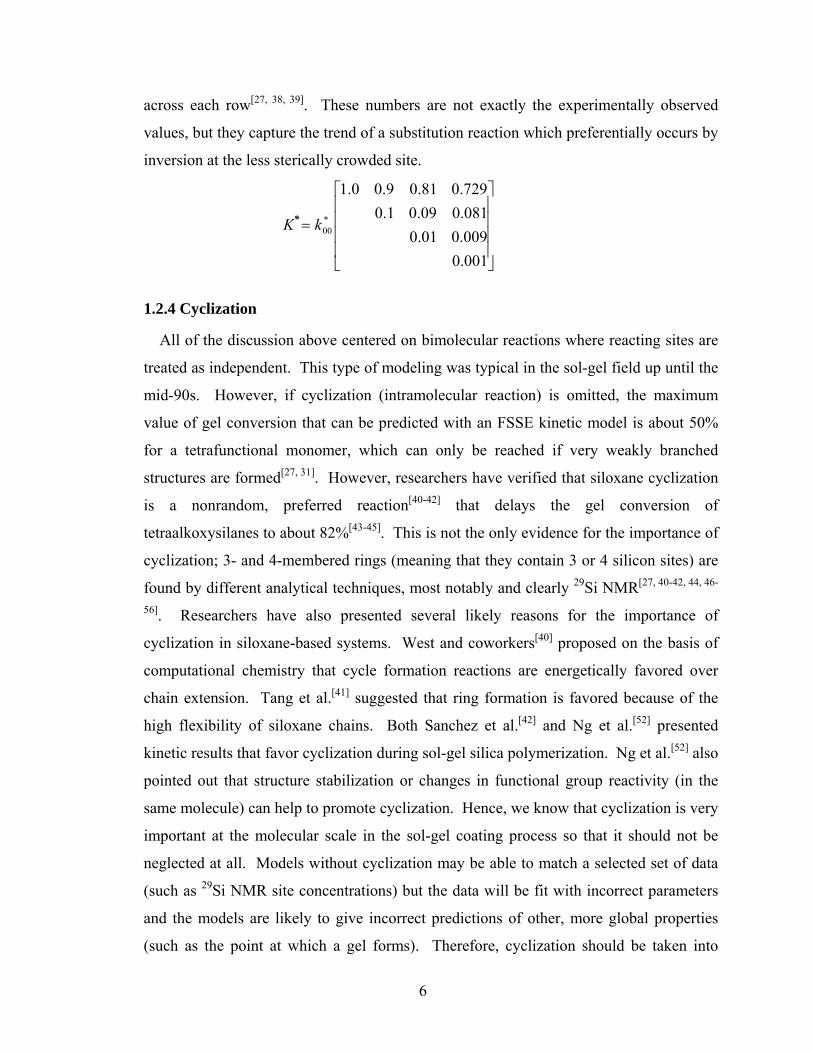
across each row[27, 38, 39]. These numbers are not exactly the experimentally observed

values, but they capture the trend of a substitution reaction which preferentially occurs by

inversion at the less sterically crowded site.

K*

⎥⎥⎥⎥

⎦

⎤

⎢⎢⎢⎢

⎣

⎡

=

001.0009.001.0081.009.01.0729.081.09.00.1

*00k

1.2.4 Cyclization

All of the discussion above centered on bimolecular reactions where reacting sites are

treated as independent. This type of modeling was typical in the sol-gel field up until the

mid-90s. However, if cyclization (intramolecular reaction) is omitted, the maximum

value of gel conversion that can be predicted with an FSSE kinetic model is about 50%

for a tetrafunctional monomer, which can only be reached if very weakly branched

structures are formed[27, 31]. However, researchers have verified that siloxane cyclization

is a nonrandom, preferred reaction[40-42] that delays the gel conversion of

tetraalkoxysilanes to about 82%[43-45]. This is not the only evidence for the importance of

cyclization; 3- and 4-membered rings (meaning that they contain 3 or 4 silicon sites) are

found by different analytical techniques, most notably and clearly 29Si NMR[27, 40-42, 44, 46-

56]. Researchers have also presented several likely reasons for the importance of

cyclization in siloxane-based systems. West and coworkers[40] proposed on the basis of

computational chemistry that cycle formation reactions are energetically favored over

chain extension. Tang et al.[41] suggested that ring formation is favored because of the

high flexibility of siloxane chains. Both Sanchez et al.[42] and Ng et al.[52] presented

kinetic results that favor cyclization during sol-gel silica polymerization. Ng et al.[52] also

pointed out that structure stabilization or changes in functional group reactivity (in the

same molecule) can help to promote cyclization. Hence, we know that cyclization is very

important at the molecular scale in the sol-gel coating process so that it should not be

neglected at all. Models without cyclization may be able to match a selected set of data

(such as 29Si NMR site concentrations) but the data will be fit with incorrect parameters

and the models are likely to give incorrect predictions of other, more global properties

(such as the point at which a gel forms). Therefore, cyclization should be taken into

7

account in the sol-gel polymerization process modeling. The details about

implementation of cyclization in dynamic Monte Carlo modeling will be given in

Chapters 4 and 5.

1.3 Dissertation Outline

This dissertation is organized as follows:

Chapter 2. Simulation Methods: There are two parts to this chapter corresponding to

the elements that are brought together in the multiscale approach used here. The first part

is about the molecular simulation technique – dynamic Monte Carlo (DMC). The second

part is about the continuum method – finite difference method (FDM) as it is applied to

the modeling of drying coating solutions. In both parts, after a review of other methods,

a description of the simulation method algorithm will be given, and an example of the

ideal polycondensation case is given for the DMC method.

Chapter 3. Multiscale Modeling of Ideal Polycondensation and FSSE: In this chapter,

two relatively simple cases are used to show ways to couple molecular and continuum

processes together. This type of coupling of modeling strategies is new in that it involves

a polymerization process that occurs throughout the entire continuum domain rather than

at a boundary. The validity of our multiscale model can be verified by the modeling the

evolution of conversion in each of these two cases. Although these cases exclude

cyclization, they can also show competition between drying and gelation, predict

different drying / gelation phenomena, and predict the occurrence of gradients of

concentration and gelation in the films. In extreme cases, gelation gradients can lead to

the formation of a gel skin near the top surface of the film, which is thought to be a site

for nucleation of defects in films such as wrinkles and cracks.

Chapter 4. Multiscale Modeling of Unlimited 3-membered Ring Cyclization: This

chapter describes the addition of cyclization reactions to our multiscale model, but only

cyclization reactions allowing the formation of 3-membered rings. This multiscale model

is the first one coupling unlimited cyclization in polycondensation with continuum mass

transfer process. It is also the first model that can predict the structure gradient

throughout drying sol-gel films, as hypothesized in earlier work with closed dynamic

Monte Carlo simulations.

8

Chapter 5. Multiscale Modeling of Unlimited 4-membered Ring Cyclization: This

chapter presents the first dynamic Monte Carlo model that can simulate unlimited 4-

membered ring cyclization. This is important because 4-membered rings are the

dominant cyclic structural units in real sol-gel silicates. Compared with 3-membered ring

cyclization, the number of potential rings in the 4-membered rings cyclization is greater

and the molecular structure of the products is more complicated with a dimensionless

cyclization tendency 5≥κ (a physically reasonable value for sol-gel polymerization). At

the same process conditions (Bi, Da and κ), films with 4-membered ring cyclization gel

more quickly, have more number-average cycle rank per molecule, and display more

extreme structure gradient than films with only 3-membered rings. The inclusion of 4-

membered rings in this chapter represents a significant advance in our ability to

quantitatively model sol-gel polymerization in thin films.

Chapter 6. Conclusions: A summary of the whole dissertation is presented along with a

brief discussion about future opportunities presented by the work that has been done so

far.

Chapters 3, 4 and 5 are under revision as journal manuscripts and will be submitted for

peer-reviewed publications soon.

9

Chapter 2

Introduction to Molecular and Continuum Simulation Methods

2.1 Molecular Modeling Technique – Dynamic Monte Carlo (DMC) Method

2.1.1 Introduction

The Monte Carlo (MC) method is a stochastic simulation technique[57]. Using random

numbers and probability, the Monte Carlo method allows one to study problems that are

difficult or impossible to solve deterministically or are encountered during the evolution

of a finite population[58]. In Monte Carlo simulations, integration is approximated

through a random event selection process which is repeated many times to create multiple

realizations of a sequence of events. Each time one event is randomly selected, it

represents a step in one possible configuration and solution to the problem. Together,

these configurations give a range of possible solutions, some of which are more probable

and some less probable. When repeated for many configurations (10,000 or more), the

average solution will give an approximate answer to the problem[58, 59]. Accuracy of this

answer can be improved by simulating more realizations of the sequence of events or, in

the case of population balance modeling, by using a larger population [58, 60]. For Monte

Carlo method, the finite size of the population is the primary source of error[58] and it

restricts the maximum simulated length scale[38, 61].

In statistical physics, Monte Carlo methods are often used to sample the configurations

of a system that contribute most to the average properties of that system. For instance, in

molecular simulations at equilibrium, a Monte Carlo method favors configurations with a

high probability of being found according to the Boltzmann distribution, rather than

calculating average properties by enumerating all possible configurations of the system of

many particles. Similarly, in a Markov chain process (a sequence of events described by

transition probabilities) such as polymerization, Monte Carlo simulations are used to

sample only the chain structures that are likely to be realized by the kinetic scheme,

10

rather than needing to enumerate and solve kinetic equations for all possible polymer

structures.

Monte Carlo simulations have been purposely used to capture the effects of

fluctuations in small systems such as micro-fluidic reactors. As early as 1976,

Gillespie[62] proposed that the Monte Carlo method can be used for simulation of

chemical kinetics in finite populations of molecules. He suggested that the Monte Carlo

method is able to handle systems in which many chemical species participate in many

highly coupled and highly nonlinear chemical reactions, and it takes full account of

fluctuations and correlations near chemical instabilities[62]. Vlachos[63] compared the

instabilities in homogeneous non-isothermal reactors (CSTR), using deterministic and

Monte Carlo methods. He suggested that the Monte Carlo method is uniquely suited to

examine thermal fluctuations and finite size effects near critical points[63].

In the last two decades, many researchers have found that Monte Carlo simulations are

very good choices to model the sol-gel silica formation process and other network

polycondensation reactions. Šomvársky and Dušek[61, 64] described a MC method for

simulation of structure evolution in branched polymer systems and discussed the system

size effect on network formation. They also discussed the disadvantages of other

methods (e.g. cascade theory, recursive theory and percolation techniques) in the

simulation of polymer network formation[61]. In contrast to the other statistically derived

methods, the MC method can capture the complete reaction history for a finite set of

monomers[61]. In particular, the additional network information such as molecular weight

distribution and cycle rank distribution can be recorded during the simulation[64], so MC

simulations can provide more accurate results than other network polymer models such as

a kinetic-recursive model[31, 39, 61]. The disadvantage of statistical approaches is that they

derive average structural characteristics by assuming random assembly of some sort of

building blocks. Even if a non-random kinetic feature such as a first-shell substitution

effect (a dependence of condensation rate on prior condensation reactions) is included,

correlations may be lost because the sites are essentially “cut up” and reassembled when

properties like average molecular weight are computed, for example by a recursive

approach. Hendrickson et al[35] studied substitution effects in four-functional sol-gel

precursors using a MC technique. They compared their results with analytical results to

11

confirm the accuracy of the MC method, and verified again that network properties can

be calculated directly from the investigation of the network connectivity[35], which is one

advantage of MC method we just mentioned. Furthermore, the MC method has the

flexibility to handle larger cycles and cages that are thought to play a significant role in

the structure of sol-gel silica[43]. Hendrickson[65], Kasehegen[39], Ng[43] and Rankin[27, 38,

66] et al. have shown how to use the Monte Carlo method to deal with cyclization

reactions in sol-gel silica polycondensation, although they each treated cyclization

somewhat differently. Compared with molecular dynamics simulations[67-69] which are

computationally intensive and have limitations in the accessible length and time scales,

dynamic Monte Carlo simulations can simulate much larger systems and much longer

times, and they are computationally efficient because each MC step is a reaction event[70].

A possible criticism of the MC approach is that kinetic parameters for the rates of

bimolecular and cyclization reactions must be input into the simulation. However, these

coefficients could hypothetically be derived from first-principles ab initio or molecular

dynamics calculations based on transition state theory.

2.1.2 DMC Algorithm

Classical random branching theory (RBT) i.e. Flory-Stockmayer theory[71-73] can

provide an adequate prediction of the average properties of network polycondensation

systems which satisfy the following ‘ideal’ assumptions[31, 43]: first, all of the functional

groups have equal and independent reactivities; second, no cyclization reactions are

allowed in the system. Here we use this ideal case as the example to illustrate the details

of the DMC algorithm, and to verify the accuracy of the present implementation of the

DMC method by comparing our simulation results with analytical results of RBT. Based

on sol-gel chemistry discussed in Chapter 1 but not considering cyclization, we need to

consider 10 condensation reactions among four differently connected silicon sites. This

is a first-shell substitution effect (FSSE) model but it becomes ideal by setting all the rate

constants equal to one another.

At the beginning of the simulation or the synthesis process, we have pure TEOS, so all

the molecules are monomers (designated as Q0 where the subscript indicates the number

of siloxane bonds attached to a site). Rij (i from 0 to 3, j from i to 3) is used to denote the

12

reaction rate for one of the 10 condensation reactions between species Qi and Qj.

Although these rates are actually the product of the concentrations of the participants and

a rate constant k, in the simulation, we calculate the reaction rates as the products of the

populations of silicon sites and the rate constants, because we are only concerned with

the relative reaction rates (for now – the concentration only becomes important when

calculating the time evolution of the system, which will be discussed when needed in

future chapters). In other words, we use are integral populations Qi to calculate Rij, and

not concentrations [Qi][35, 61].

2.1.2.1 Data Structures

In the Monte Carlo simulation, we need to record a variety of information about the

progress of the polycondensation process, such as the populations of silicon atoms with

differing connectivities, molecular tags, the sizes of molecules, the molecule membership

of the silicon atoms, and so on. The information contained in the data structures is

updated after each step (reaction) for later interrogation. The data structures allow

specific species to be selected randomly from the entire population when species of a

particular type are needed to take part in a reaction.

The data structures used in the algorithm are as follows:

1) Silicon sites arrays: we use two one-dimensional arrays to store the information

about silicon sites (Q species). One records the numbers of each type of Q species (Qi),

while the other is used to index the silicon sites. Each element of the latter array is a data

structure, in which the information about molecular tag and membership is stored. The

details are provided below.

2) Molecular tags [35]: this array is used to identify the molecules. An integer tag is

assigned to each molecule. In the beginning, all of the monomers have different

molecular tags because they are unconnected to one another. In the bimolecular reaction,

the product molecule is tagged with the tag of larger reactant molecule. All of the

monomers (sites) on the same molecule have the same integer tag.

3) Membership: we keep track of molecule membership using four pointers to the four

neighbors connected to each silicon site, indexed by silicon site number. The pointers are

set to NULL for monomers. When a reaction occurs, a bond is formed between two sites,

13

and for each reactant site, one pointer to its new neighbor (the other reacting site) is

added.

4) Size array [35]: we use this array to record the sizes of molecules in the system. In

the beginning, the sizes of monomers are all set to 1. Using molecular tags as indices, in

the bimolecular reaction, the length of the larger molecule is updated to be the sum of the

sizes of the two reactants, while the length of the smaller one is set to zero.

5) Size distribution array: a linked list is used to keep track of the molecular weight

distribution in the simulation. Each element of the linked list contains the information of

molecular size, the number of molecules having this size and the pointer to the next

member in the size distribution array.

6) Conversion: in the DMC simulation, because conversion is the fraction of functional

groups that have condensed, it can be calculated as follows [35]:

NS

SiOSiSi

groupsfunctionalofmoltotalgroupsfunctionalcondensedofmolα t

××

=−

==42

][4][ , (2.1)

where St is the total number of DMC steps, and N is the total number of monomers.

7) Gel point: In DMC simulations, the gel point can be estimated by the divergence of

the weight-average degree of polymerization (DPw)[38]. DPw can be calculated directly

from the molecular weight distribution as[38, 64]:

∑=

=molN

iw iL

NDP

1

2)(1 , (2.2)

where L(i) is the size of the molecules in the population, and N is the total number of sites.

A better way to find the value of gel conversion is to plot the reduced weight averaged

degree of polymerization (rDPw) against conversion[38, 74]. rDPw can be calculated by

removing the largest molecule from the molecular weight distribution in the DMC

simulation and recalculating DPw[64]:

max

2max

1

2 )()(

LN

LiLrDP

molN

iw −

−=∑= , (2.3)

where Lmax is the size of the largest molecule in the population. Below the gel point,

w wrDP DP= ; but rDPw drops sharply at gelation[64]. Therefore the value of conversion at

gelation can be determined by the position of the peak in rDPw.

14

2.1.2.2 Monte Carlo Reaction Selection

Monte Carlo reaction selection is used to make sure that reactions compete properly

according to their relative rates. In Monte Carlo simulation, the rates are normalized into

a set of probabilities Pij which (for bimolecular reactions only) are given by [35, 39]:

∑∑= ≥

= 3

0

3

i ijij

ijij

R

RP . (2.4)

A random number r is used to choose a reaction. In our program, it is calculated based

on a pseudo-random number generator – the ANSI C rand() function:

MAXRANDrandr _/()0.1 ×= . (2.5)

In order to produce floating point numbers uniformly distributed over the interval (0, 1),

we recalculate Eq. (2.5) if r is equal to 0 or 1. After a number is picked, the summation

of probabilities is started in the sequence P00, P01, P02, etc. until the partial sum exceeds

the random number. That is, if ),(),( 2211 jisumrjisum ≤< , we choose the i1j1-th

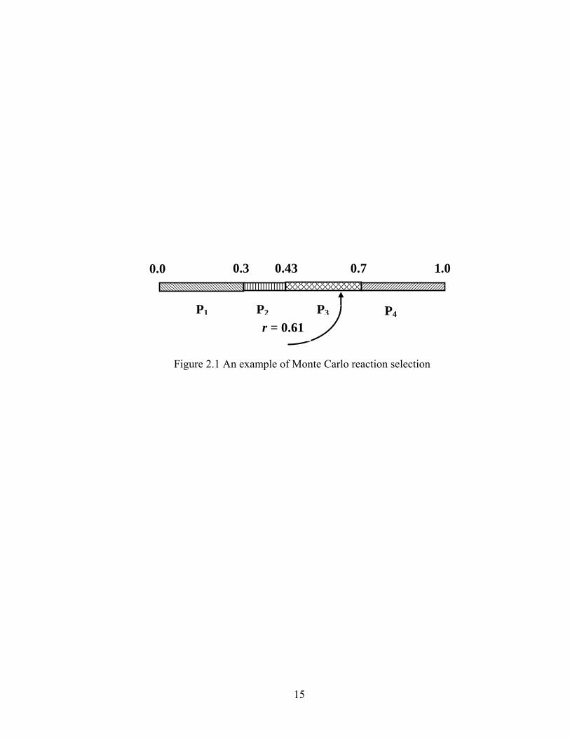
reaction. As a simple example shown in Figure 2.1, if P = 0.3, 0.13, 0.27, 0.3, and the

random number is equal to 0.61, then reaction 3 is chosen. Finally, after the reaction is

selected, it is executed. For bimolecular reactions, this means that two sites to react are

chosen from the populations of all sites with the appropriate connectivities for the chosen

reaction. The chosen sites are joined, and arrays are adjusted to reflect the change in

state of the system. At the next step, the reaction rates and probabilities are updated and

a new reaction is selected. The reaction rates and reaction probabilities are respectively

stored as 4×4 matrices.

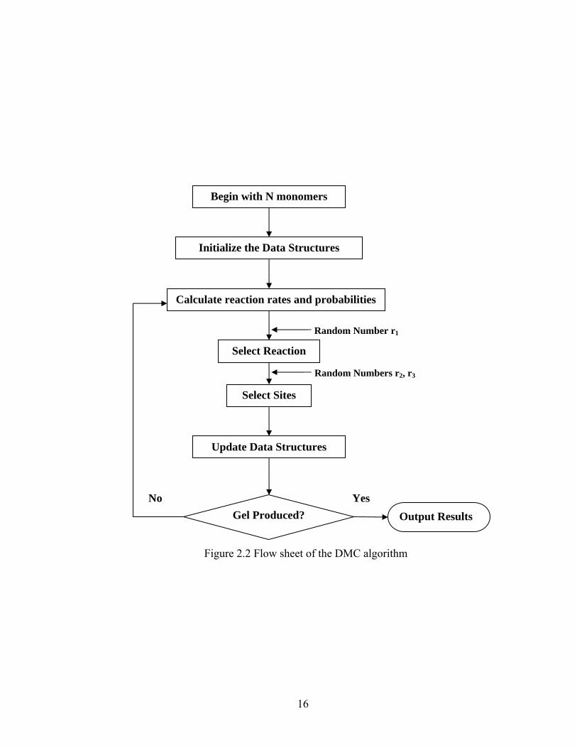
2.1.2.3 Flow Sheet

A flow sheet of the algorithm is given in Figure 2.2. At each DMC step, one siloxane

bond is added to the population of monomers. This is an advantage of this algorithm in

comparison with other Monte Carlo algorithms based on randomly selecting reactions

and deciding whether to accept them based on acceptance probabilities. Our approach is

sometimes called the “continuous time Monte Carlo” method because it is based not on

discretizing time intervals but on discretizing reaction events. Because no bond additions

attempts are rejected, this approach is very efficient, as we mentioned before. We begin

15

Figure 2.1 An example of Monte Carlo reaction selection

0.0 0.3 0.43 0.7 1.0

P1 P2 P3 P4 r = 0.61

16

Figure 2.2 Flow sheet of the DMC algorithm

Begin with N monomers

Initialize the Data Structures

Calculate reaction rates and probabilities

Select Reaction

Select Sites

Update Data Structures

Gel Produced?

Random Numbers r2, r3

Random Number r1

Output Results No Yes

17

with N monomers, initialize the data structures, and then we start the reaction steps. At

each reaction step, we can calculate the reaction rates based on the current population of

reactive species, and then obtain the probabilities according to all of the rates[39]. One

reaction is selected by a random number and reactive sites are also chosen by two random

numbers. Then the reaction is executed and the data structures are updated accordingly.

The whole process for each reaction step is repeated until a stopping criterion is met

(which is chosen to be after the gel point – for instance, once DPw reaches a value greater

than 10% of the total number of monomers, finite size effects become important and so

the simulation is stopped).

2.1.3 Random Branching Theory (RBT)

Based on the RBT, conversion at gelation can be expressed as[71]

1( 1)g f

α =−

. (2.6)

where f is the functionality. For the acid-catalyzed TEOS system 4f = , so we could infer

that gelation is expected to occur when the conversion reaches 1/3 in the ideal case. In

addition, DPw can be predicted in the ideal case to be[64, 75]:

1 11 ( 1) 1 3wDP

fα α

α α+ +

= =− − −

. (2.7)

If we keep track of the number of silicon species with differing connectivity i (Qi), it is

expected to be a function of the siloxane bond conversionα . In the ideal case, the

analytical solutions for the fractions of different Qi species as functions of conversion can

be derived based on the assumption of equal reactivity, from which it follows that (1-α)

is the probability that any of the ligands attached to a site has not polymerized.

Combinatorial considerations lead to the following expressions[75]:

40( ) (1 )f Q α= − , (2.8)

31( ) 4 (1 )f Q α α= − , (2.9)

2 22( ) 6 (1 )f Q α α= − , (2.10)

33( ) 4 (1 )f Q α α= − . (2.11)

18

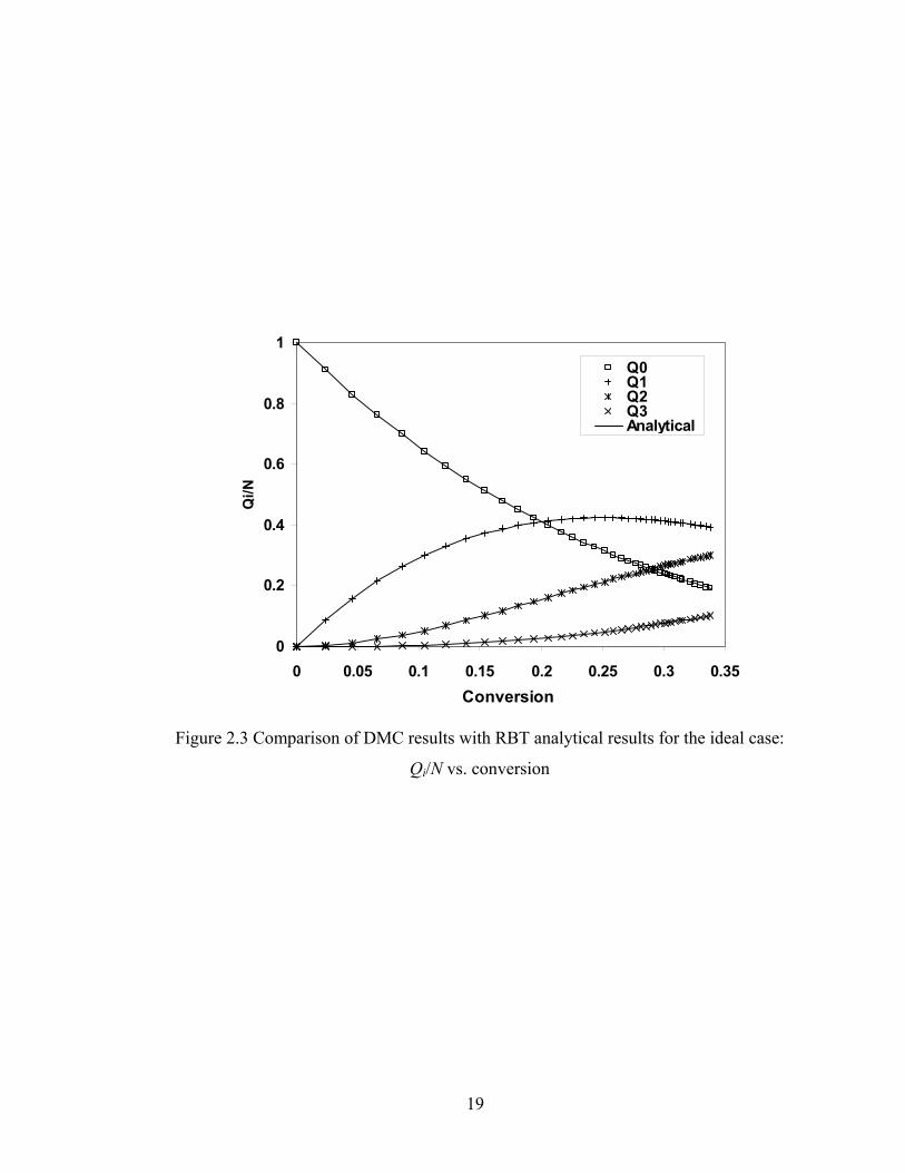
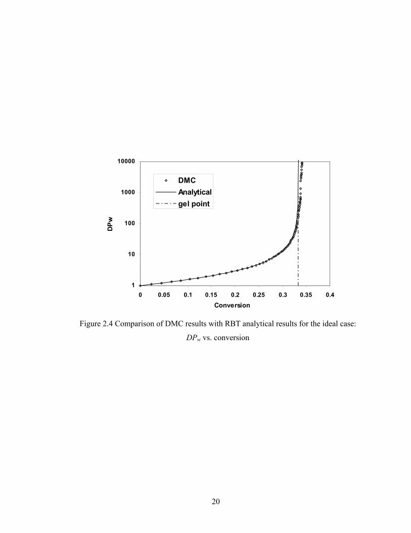
2.1.4 Results and Discussion

In our DMC test simulations discussed here, we use 1.0E+05 monomers. The

accuracy of the DMC method can be verified by comparing the simulation results with

analytical results based on RBT. Figure 2.3 shows the number fractions of different Qi

species as a function of conversion. The DMC results (points) are very consistent with

the analytical equations above (curves). Figure 2.4 presents the comparison of weight-

average degree of polymerization for DMC simulations and RBT. It is clear that the

tendency of the DPw of DMC is correct until the gel conversion is approached. We can

also find that above the gel point the deviation between simulation and analytical solution

grows rapidly. This is a finite-size effect[64] and it is normal for MC simulations.

Because of the finite size of the population of polymers, a deviation is expected to happen

late in reaction, but usually it does not begin until DPw is at least 1% of the total number

of monomers, and usually is not severe until it is 10% of the total number of monomers.

Based on Figures 2.3 and 2.4, DMC method is proven to be accurate to simulate the sol-

gel polycondensation process.

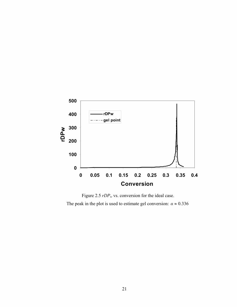
As we mentioned above, a plot of reduced weight averaged degree of polymerization

(rDPw) against conversion can also used to find the value of gel conversion. Figure 2.5

shows an example of using the peak in a plot of rDPw against conversion to estimate the

gel conversion. For this case, we estimate the gel conversion to be about 0.336, which is

almost the same as the analytical solution.

2.2 Continuum Modeling Method – Finite Difference Method (FDM)

2.2.1 Introduction

As discussed in Chapter 1, modeling sol-gel film formation requires a multiscale

approach that combines the granular, molecular description of polymerization given by

the DMC method with a continuum model of the drying process. Researchers have

shown that the finite difference method (FDM) can correctly model the drying process of

polymer films. Blandin et al.[76] presented a film drying model based on FDM, which

gives results in good agreement with experimental data, thus validating the model.

Vrentas et al.[77] proposed using FDM to solve a set of equations which describe heat and

mass transfer and film shrinkage in the drying of polymer films. Alsoy and Duda[78]

19

0

0.2

0.4

0.6

0.8

1

0 0.05 0.1 0.15 0.2 0.25 0.3 0.35Conversion

Qi/N

Q0Q1Q2Q3Analytical

Figure 2.3 Comparison of DMC results with RBT analytical results for the ideal case:

Qi/N vs. conversion

20

1

10

100

1000

10000

0 0.05 0.1 0.15 0.2 0.25 0.3 0.35 0.4

Conversion

DPw

DMCAnalyticalgel point

Figure 2.4 Comparison of DMC results with RBT analytical results for the ideal case:

DPw vs. conversion

21

0

100

200

300

400

500

0 0.05 0.1 0.15 0.2 0.25 0.3 0.35 0.4

Conversion

rDPw

rDPwgel point

Figure 2.5 rDPw vs. conversion for the ideal case.

The peak in the plot is used to estimate gel conversion: 336.0≈α

22

applied their model, which is based on the model of Vrentas[77] and solved by the finite

difference approximation, to the well characterized polyvinylacetate (PVAC)-toluene

system. Two sets of data available for the drying of polystyrene (PS)-toluene and PVAC-

toluene systems verify the validity of the model[78]. Kuznetsov et al.[79] utilized FDM to

solve their model which describes the effect of evaporation on the free surface profile and

solute concentration distribution. Lou and coworkers[80] demonstrated that a model

solved by FDM can provide satisfactory long-term predictions of film formation.

The purpose of the work described in this dissertation is to develop a relatively simple,

but sufficiently accurate method to model the moving boundary drying process in the sol-

gel silica films. As will be discussed in later chapters, this model is to be coupled with

the DMC model to give a comprehensive, multiscale approach. Compared with other

methods that have been used to model the drying process of polymer solutions such as

integral approach[81] and finite element method[82-85], FDM is easy and intuitive to

implement, which is advantageous for developing multiscale methodology. In the

following section, the FDM algorithm is briefly introduced. More details about our

drying model (including the continuum equations) to be solved using FDM will be shown

in Chapter 3.

2.2.2 FDM Algorithm

The FDM is a simple and efficient method for solving ordinary differential equations

(ODEs) and partial differential equations (PDEs) in domains with simple boundaries.

The method is based on substituting of derivatives in the differential equations by finite

difference approximations[86]. These basic approximations are based on the definition of

the derivative,

h

xfhxfxfDh

)()(lim)(0

−+≡

→+ (2.12)

provided that the limit exists. We just delete the limit operation in order to obtain a

finite-difference approximation to )(xfD+ . The result is known as the first forward

difference,

hxfhxfxfD )()()( −+

≈+ , (2.13)

or,

23

ii

iiii

xxff

hffxfD

−−

=−

≈+

+++

1

11)( , (2.14)

where 1i ix x h+ = + and the subscripts here denote different points in the grid defining the

FDM modeling domain.

If h is sufficiently small and 2f C∈ in a neighborhood of ix x= , the accuracy of the

first forward difference can be obtained using a Taylor series about the point xi

…+⋅′′

+⋅′+=+2

1 2hfhfff i

iii (2.15)

Substituting (2.15) into (2.14), we have

…… +⋅′′

+′=⎥⎦

⎤⎢⎣

⎡−⎟

⎠⎞

⎜⎝⎛ +⋅

′′+⋅′+=

−+ hfffhfhffhh

ff iii

iii

ii

221 21 (2.16)

So the leading error of Eq. (2.16) is 2

if h′′⋅ and the approximation is first order accurate

with respect to the step size h.

There are two other approximations: backward-difference approximation and centered-

difference approximation. Using the same procedure we can see that backward-

difference approximation is also of first order accuracy, while the centered-difference

approximation is of second order accuracy with respect to the step size h. Therefore, the

centered-difference approximation is more accurate, and it is the approximation that we

will use in our continuum modeling.

Backward-difference approximation: )()( 1 hOfh

ffhfD iii +′=

−= −

− (2.17)

Centered-difference approximation: )(2

)( 2110 hOf

hffhfD i

ii +′=−

= −+ (2.18)

The approximation of higher order derivatives by the finite difference method can also

be obtained using the similar approach. For example, the centered-difference

approximation of a second order derivative can be derived as follows:

⎟⎠⎞

⎜⎝⎛ −

== −+−+ h

ffDhfDDhfD ii 120 )()(

( )11

−++ −= ii fDfDh

24

⎟⎠⎞

⎜⎝⎛ −

−−

= −+

hff

hff

hiiii 111

( )112 21−+ +−= iii fff

h

)( 2hOfi +′′= (2.19)

2.2.2.1 Discretization (grid)

The FDM requires that the domain is discretized to form a grid. At each grid point

each term in the differential equation is replaced by a difference formula which may

include the values of function at that point and its neighboring grid points. By

substituting the difference formula into the equation, a difference equation is obtained.

The grid is formed by the partition of the domain consisting of M×N points, and the grid

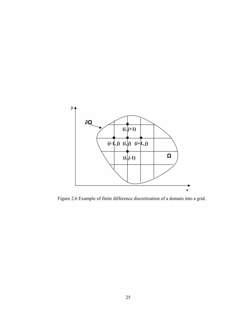
points are indicated in Figure 2.6. In our cases, we use a uniform spacing for the

computational mesh, using j index as time and i index as position.

2.2.2.2 Explicit Scheme

The PDEs are transformed to finite difference equations after the finite difference

approximations replace the derivatives. These finite difference equations can be solved

either by explicit or implicit method. In the explicit scheme, the modeled variable values

at a new time can be directly calculated from the previous ones. Therefore in this

approach, the PDE can be solved directly using the boundary conditions. In contrast, an

iterative process is used to calculate modeled variable values at a new time in an implicit

scheme. A trial solution is input as a first guess to the equations, and a new solution is

calculated and used as new input in each iteration until the values converge to within a

specified tolerance[87]. Because of their iterative nature, implicit schemes are usually

more numerically intensive than explicit methods, although the increased accuracy they

provide is required for some problems. It is clear that an explicit scheme is much easier

to implement and debug than the implicit scheme. Therefore, we will use explicit FDM

in our continuum modeling because our one-dimensional drying model is amenable to a

simplified approach.

25

Figure 2.6 Example of finite difference discretization of a domain into a grid.

Ω

(i, j)

(i, j-1)

(i-1, j) (i+1, j)

(i, j+1) ∂Ω

x

y

26

2.3 Summary

This chapter presented a general overview of the simulation methods used in this

dissertation: the DMC method for molecular simulation and FDM for continuum

modeling. DMC simulation is a very good choice to model the sol-gel silica

polycondensation because it can capture the complete reaction history for a finite set of

monomers, it has the flexibility to handle new types of reactions associated with the

formation of large polycyclic species and cages, and it can simulate much larger systems

and much longer times than competing molecular approaches such as molecular

dynamics. The accuracy of DMC as we have implemented it can be verified by the good

agreement between simulation results and analytical results (based on RBT) for the ideal

polycondensation case. The FDM is an easy and intuitive numerical method to model the

drying process of sol-gel silica films. Because we use a one dimensional model to

develop the multiscale approach, FDM should provide adequate numerical accuracy and

precision for the purposes of this dissertation. There are many examples to show that

FDM can correctly model the drying process of polymer films. More details about our

continuum modeling using explicit FDM will be shown in Chapter 3, including the

balance equations, approach to nondimensionalizing the equations, boundary conditions,

and coupling to the DMC simulation.

27

Chapter 3

Multiscale Modeling of Ideal Polycondensation and Polycondensation with First

Shell Substitution Effect (FSSE) in Drying Thin Films

3.1 Introduction

Modeling silica curing in drying films is important for overcoming challenges in

controlling the thickness, cracking and homogeneity of the films. Until now, most

models of sol-gel polymerization or drying polymer films have provided useful insights

into the essence of the physical phenomena, but they only focused on selected length and

time scales. For example, kinetic models of the gelation behavior of silica

polymerization have been developed using recursive statistical techniques or Monte Carlo

simulation[31, 38, 39, 75]. These modeling approaches are necessary to link rates of

polymerization of individual monomers to molecular weight distributions and gelation of

branched polymers. On the other hand, drying has been approached using continuum

models and solved with an integral approach[81], finite element method[82-84] or finite

difference method[76-78, 80]. However, during the formation of sol-gel coatings, both

polymerization and drying occur simultaneously, so the process involves multiple length

and time scales ranging from molecular to macroscopic.

Unlike other processes where multiscale models have previously been applied, the sol-

gel polycondensation occurs throughout the thickness of the film where solvent transport

is occurring. Therefore, it is not possible to regard the polymerization reaction as

occurring in a place spatially separate from the place where the coating flow occurs. At

the molecular level, polymerization and (if surfactants are added) self-assembly process

occur which control the film properties such as film microstructure. At the same time,

the formation of the film is controlled by macroscopic parameters. Diffusion and mass

transport occur over micron or greater length scales, and define the concentration fields

within which polymerization and self-assembly occur. Therefore, we are challenged in

this process to develop a methodology to link different length and time scales together

throughout the entire simulated domain.

28

In this chapter we present a multiscale model which captures the evolution of both

macroscopic and molecular phenomena of this sol-gel silica film formation process. The

process of diffusion and mass transport can be adequately modeled by treating the film as

a continuum. The macroscopic conservation equations for mass are expressed by a set of

partial differential equations for species concentration with initial and boundary

conditions. Based on finite difference method, the continuous domain is discretized and

these PDEs are solved numerically. However, at the molecular length scale, the

continuum hypothesis is no longer valid and the molecular phenomena cannot be

described by deterministic PDEs[21]. At such a small length scale, the kinetics of sol-gel

polymerization is best modeled by dynamic Monte Carlo (DMC) simulation. This

approach is necessary because of the nonideal nature of silane polymerization (which

precludes the use of random branching theory[71-73] and even throws into question the

validity of statistical techniques such as the kinetic-recursive method[31, 39]). DMC

simulations can simulate much longer times and much larger ensembles than molecular

dynamics simulations[38, 70] can and have the potential flexibility of handling larger cycles

and cages that are thought to play a significant role in the structure of sol-gel silica[38, 43,

66]. The inclusion of these cyclization reactions will be the subjects of the next two

chapters, but here we focus on the coupled DMC / continuum model.

We will begin by describing the model integrating the DMC method and continuum

model, as well as the physical assumptions and the simulation procedure. We first briefly

review DMC simulation, since we have discussed sol-gel silica chemistry in Chapter 1

and presented the DMC algorithm in Chapter 2. Details are given about how to calculate

the time interval in the DMC model. In the continuum model, the entire DMC simulation

(containing ~ 106 monomers) is treated as a particle of sol whose position and

composition are tracked using diffusion / evaporation finite difference calculations.

Linking the two models is accomplished by tracking the positions of sol particles during

drying. In the third section, two specific cases are considered – ideal polymerization and

polymerization with a first shell substitution effect (FSSE). The effects of concentration

gradients during drying are captured by simulating swarms of particles starting from

different positions in the film. By varying process parameters, we observe their effects

on the competition between drying and gelation, predict different drying / gelation

29

phenomena, and predict the occurrence of gradients of concentration and gelation in the

films which can lead to the formation of a gel skin near the top surface of the film.

3.2 DMC Model

The DMC model is solved based on the following assumptions: only a first shell

substitution effect for condensation is considered, hydrolysis is assumed to be at

pseudoequilibrium, alcohol-producing condensation is neglected and no cyclization is

allowed. With this set of assumptions, a finite set of N monomers (N ~ 2.5×106) is

polymerized in a manner consistent with the kinetics described in Chapter 1 by a DMC

approach. The set of bimolecular condensation reactions is as follows:

*

1 1 2ijk

i j i jQ Q Q Q H O+ ++ ⎯⎯→ + + , (3.1)

where Qi represents a tetrafunctional silicon site with i siloxane bonds (where i represents

the number of linkages to other silicon atoms), and both i and j can vary between 0 and

3[38]. Assuming that hydrolysis reaches quasi-equilibrium with constant χ , the rate of

reaction (3.1) can be expressed as:

⎪⎩

⎪⎨⎧

=−−

≠−−=

jiQQjfifk

jiQQjfifkR

jiij


21

],][)[)((*

*

(3.2)

where [Qi] represents the concentration of silicon sites Qi[39].

In the simulation, each monomer unit is indexed as a separate entity. At each DMC

step, one siloxane bond is added and the conversion (α ) is increased by a small constant

value αΔ , as given by:

7100.221

42Δ −×==×

=NN

α , (3.3)

where N is the total number of sites.

At each step, the probabilities Pij of selecting each type of condensation reaction are

evaluated by calculating the rates of the reactions, and one reaction is chosen to occur.

After selecting a reaction, the particular sites joining in the reaction are randomly chosen

from the subset of sites fitting to the required characteristics – in this case, that the sites

have the correct connectivities chosen for the reaction. After the sites are chosen, they

30

are joined with one siloxane bond and all information is updated. DMC steps are

repeated until a stopping criterion is met.

One thing that needs to be emphasized here is the calculation of the time interval[62, 70]

during each bond addition, which is given by:

1lnSi ij

NtC R r

⎛ ⎞Δ = ⋅ ⎜ ⎟⎝ ⎠∑

, (3.4)

where N is the total number of sites, r is a random number chosen from (0, 1), and Rij is

the rate described by Eq. (3.2) but based on the populations of silicon sites Qi in the DMC

model, rather than the concentrations [Qi][35]. In this equation, CSi is the total silicon site

concentration which comes from the continuum model at the time that the reaction is

selected. This concentration serves as one link that allows us to synchronize our DMC

model and the continuum model in this multiscale process. We will give more details in

the following description of the continuum model.

One of the important results we need to obtain from the DMC simulation is the gel

point. We know that a gel is a sample-spanning polymer network. In theory we can use

an infinite molecular weight polymer to represent the gel[31]. In the DMC simulation, the

gel point can be estimated by the point at which DPw diverges, or could be better

determined using the peak of rDPw[38, 39]. DPw is the weight-averaged degree of

polymerization, and rDPw is the reduced weight-averaged degree of polymerization,

which is calculated by removing the largest molecule (the gel) from the population and

recalculating DPw.

Here, we will simulate two cases with the DMC model – an ideal polymerization case

and a FSSE case. In the ideal polymerization case, the functional groups will react

randomly and independently, which means that all the rate constants are equal to each

other and no cyclization exists. In the FSSE case, we consider non-ideal polymerization

effects, but still exclude cyclization. The rate coefficients of the FSSE case are set to

drop by 10% across each row and to decrease by 90% down the diagonal, which

resembles the experimental substitution effect[38]. In other words, *00

*01 9.0 kk = ,

*00

*02 81.0 kk = , etc. while *

00*11 1.0 kk = , *

00*22 01.0 kk = , etc. In fact, the ideal case represents

a particular case of a FSSE model in which the set of connectivity-dependent rate

coefficients are all set equal to one another.

31

3.3 Continuum Drying Model

3.3.1 Model Assumptions and Description

The continuum model for the formation of sol-gel thin-film coatings is described by

macroscopic conservation equations for mass. It is a simplified one-dimensional model

corresponding to a rapidly deposited film that begins drying and curing after the coating

process is complete. Via evaporation, solvent is removed continuously at the top liquid /

vapor interface. In addition to this evaporation, the diffusion of solvent within the film

and the chemical reactions of dissolved species need to be included in this model. A

schematic diagram of the sol-gel film drying process is given in Figure 3.1.

To facilitate the modeling, the following major assumptions are used here:

1) The film is extremely thin as compared with the surface area so that concentration

variation is assumed to occur only in the thickness direction.

2) The concentrations of species are uniform throughout the film at the beginning of

the drying process.

3) The solid substrate supporting the thin film is taken to be impermeable.

4) At the surface of the coating the vapor is in equilibrium with the coating, and the

pressure in the gas phase is effectively uniform.

5) The evaporation rate of the solvent from the surface is proportional to the difference

in gas-phase mole fraction of solvent between the vapor just above the surface of the film

and the bulk gas.

6) The process is isothermal, i.e. heat transfer effects are not considered here.

7) The diffusion coefficients of solvent and sol are assumed to be constant and equal,

and the cross-term diffusion coefficients are set to zero.

8) Hydrolysis is assumed to achieve quasi-equilibrium before the drying process is

started and hydrolysis extent 1=χ .

9) Alcohol has already evaporated before the drying process is started and there is

excess water in the solution. That means we can consider just water as the solvent.

10) The film thickness changes are assumed to be dominated by solvent evaporation so

that volume changes due to reactions can be ignored.

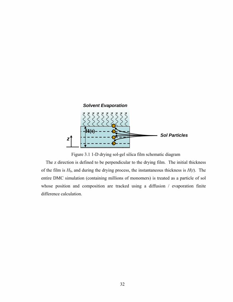
32

Figure 3.1 1-D drying sol-gel silica film schematic diagram

The z direction is defined to be perpendicular to the drying film. The initial thickness

of the film is H0, and during the drying process, the instantaneous thickness is H(t). The

entire DMC simulation (containing millions of monomers) is treated as a particle of sol

whose position and composition are tracked using a diffusion / evaporation finite

difference calculation.

H(t) z

Sol Particles

Solvent Evaporation

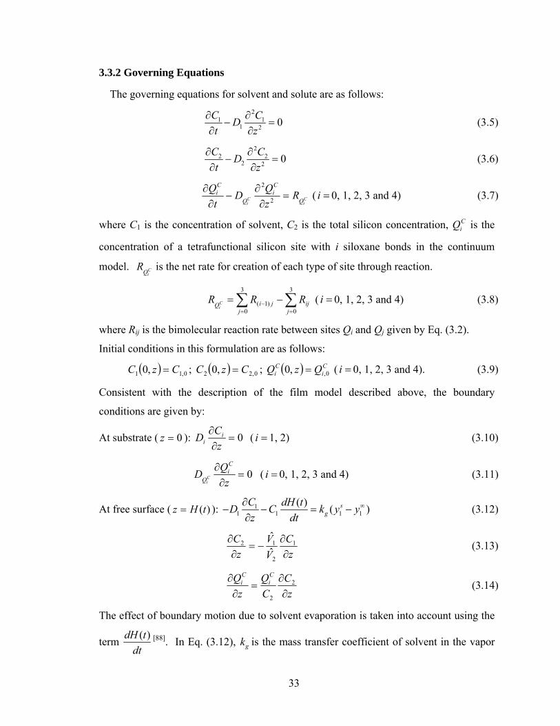
33

3.3.2 Governing Equations

The governing equations for solvent and solute are as follows: 2

1 11 2 0C CD

t z∂ ∂

− =∂ ∂

(3.5)

22 2

2 2 0C CDt z

∂ ∂− =

∂ ∂ (3.6)

Ci

Ci Q

Ci

Q

Ci R

zQD

tQ

=∂∂

−∂∂

2

2

( =i 0, 1, 2, 3 and 4) (3.7)

where C1 is the concentration of solvent, C2 is the total silicon concentration, CiQ is the

concentration of a tetrafunctional silicon site with i siloxane bonds in the continuum

model. CiQ

R is the net rate for creation of each type of site through reaction.

∑∑==

− −=3

0

3

0)1(

jij

jjiQ

RRR Ci

( =i 0, 1, 2, 3 and 4) (3.8)

where Rij is the bimolecular reaction rate between sites Qi and Qj given by Eq. (3.2).

Initial conditions in this formulation are as follows:

( ) 0,11 ,0 CzC = ; ( ) 0,22 ,0 CzC = ; ( ) Ci

Ci QzQ 0,,0 = ( =i 0, 1, 2, 3 and 4). (3.9)

Consistent with the description of the film model described above, the boundary

conditions are given by:

At substrate ( 0=z ): 0=∂∂

zCD i

i ( =i 1, 2) (3.10)

0=∂∂

zQD

Ci

QCi

( =i 0, 1, 2, 3 and 4) (3.11)

At free surface ( )(tHz = ): 11 1 1 1

( ) ( )sg

C dH tD C k y yz dt

∞∂− − = −

∂ (3.12)

zC

VV

zC

∂∂

−=∂∂ 1

2

12

ˆˆ

(3.13)

zC

CQ

zQ C

iCi

∂∂

=∂∂ 2

2

(3.14)

The effect of boundary motion due to solvent evaporation is taken into account using the

term ( )dH tdt

[88]. In Eq. (3.12), gk is the mass transfer coefficient of solvent in the vapor

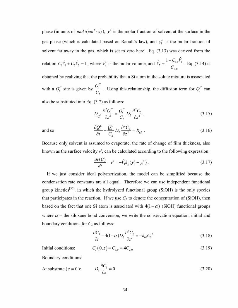
34

phase (in units of )/( 2 scmmol ⋅ ), 1sy is the molar fraction of solvent at the surface in the

gas phase (which is calculated based on Raoult’s law), and 1y∞ is the molar fraction of

solvent far away in the gas, which is set to zero here. Eq. (3.13) was derived from the

relation 1ˆˆ2211 =+ VCVC , where iV is the molar volume, and

0,2

10,12

ˆ1ˆC

VCV

−= . Eq. (3.14) is

obtained by realizing that the probability that a Si atom in the solute mixture is associated

with a CiQ site is given by

2CQC

i . Using this relationship, the diffusion term for CiQ can

also be substituted into Eq. (3.7) as follows:

22

2

22

2

2

zCD

CQ

zQD

Ci

Ci

QCi ∂

∂=

∂∂ , (3.15)

and so CiQ

Ci

Ci R

zCD

CQ

tQ

=∂∂

−∂∂

22

2

22

. (3.16)

Because only solvent is assumed to evaporate, the rate of change of film thickness, also

known as the surface velocity vs, can be calculated according to the following expression:

1 1 1( ) ˆ ( )s s

gdH t v V k y y

dt∞= = − − , (3.17)

If we just consider ideal polymerization, the model can be simplified because the

condensation rate constants are all equal. Therefore we can use independent functional

group kinetics[36], in which the hydrolyzed functional group (SiOH) is the only species

that participates in the reaction. If we use C3 to denote the concentration of (SiOH), then

based on the fact that one Si atom is associated with )1(4 α− (SiOH) functional groups

where α = the siloxane bond conversion, we write the conservation equation, initial and

boundary conditions for C3 as follows:

2

23 22 00 324(1 )C CD k C

t zα∂ ∂

− − = −∂ ∂

(3.18)

Initial conditions: ( )3 3,0 2,00, 4C z C C= = (3.19)

Boundary conditions:

At substrate ( 0=z ): 33 0CD

z∂

=∂

(3.20)

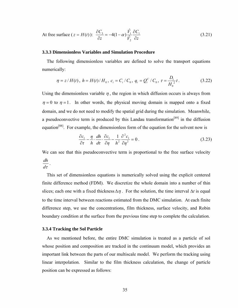
35

At free surface ( )(tHz = ): z

CVV

zC

∂∂

−−=∂∂ 1

2

13

ˆˆ

)1(4 α (3.21)

3.3.3 Dimensionless Variables and Simulation Procedure

The following dimensionless variables are defined to solve the transport equations

numerically:

)(/ tHz=η , 0/)( HtHh = , 0/ CCc ii = , 0/ CQq Cii = , 1

20

D tH

τ = . (3.22)

Using the dimensionless variable η , the region in which diffusion occurs is always from

0η = to 1η = . In other words, the physical moving domain is mapped onto a fixed

domain, and we do not need to modify the spatial grid during the simulation. Meanwhile,

a pseudoconvective term is produced by this Landau transformation[89] in the diffusion

equation[88]. For example, the dimensionless form of the equation for the solvent now is

0121

2

211 =

∂∂

−∂∂⋅⋅−

∂∂

ηc

hηc

τddh

hη

τc . (3.23)

We can see that this pseudoconvective term is proportional to the free surface velocity

dhdτ

.

This set of dimensionless equations is numerically solved using the explicit centered

finite difference method (FDM). We discretize the whole domain into a number of thin

slices; each one with a fixed thickness ηΔ . For the solution, the time interval ∆t is equal

to the time interval between reactions estimated from the DMC simulation. At each finite

difference step, we use the concentrations, film thickness, surface velocity, and Robin

boundary condition at the surface from the previous time step to complete the calculation.

3.3.4 Tracking the Sol Particle

As we mentioned before, the entire DMC simulation is treated as a particle of sol

whose position and composition are tracked in the continuum model, which provides an

important link between the parts of our multiscale model. We perform the tracking using

linear interpolation. Similar to the film thickness calculation, the change of particle

position can be expressed as follows:

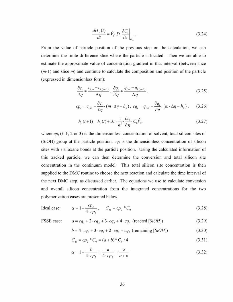
36

pH

p

zCDV

dttdH

∂∂

⋅= 111

)(. (3.24)

From the value of particle position of the previous step on the calculation, we can

determine the finite difference slice where the particle is located. Then we are able to

estimate the approximate value of concentration gradient in that interval (between slice

(m-1) and slice m) and continue to calculate the composition and position of the particle

(expressed in dimensionless form):

, ,( 1)i m i mi c ccη η

−−∂≈

∂ Δ, , ,( 1)i m i mi q qq

η η−−∂

≈∂ Δ

, (3.25)

)Δ(, pi

mii hηmηcccp −⋅⋅∂∂

−= , )Δ(, pi

mii hηmηqqcq −⋅⋅∂∂

−= , (3.26)

10 12

1 ˆ( 1) ( )p pch t h t d C V

hτ

η∂

+ = + ⋅ ⋅ ⋅∂

, (3.27)

where cpi (i=1, 2 or 3) is the dimensionless concentration of solvent, total silicon sites or

(SiOH) group at the particle position, cqi is the dimensionless concentration of silicon

sites with i siloxane bonds at the particle position. Using the calculated information of

this tracked particle, we can then determine the conversion and total silicon site

concentration in the continuum model. This total silicon site concentration is then

supplied to the DMC routine to choose the next reaction and calculate the time interval of

the next DMC step, as discussed earlier. The equations we use to calculate conversion

and overall silicon concentration from the integrated concentrations for the two

polymerization cases are presented below:

Ideal case: 2

3

41

cpcp⋅

−=α , 02 *CcpCSi = (3.28)

FSSE case: 4321 432 cqcqcqcqa ⋅+⋅+⋅+= (reacted [SiOH]) (3.29)

3210 234 cqcqcqcqb +⋅+⋅+⋅= (remaining [SiOH]) (3.30)

4/*)(* 002 CbaCcpCSi +== (3.31)

ba

acpa

cpb

+=

⋅=

⋅−=

22 441α (3.32)

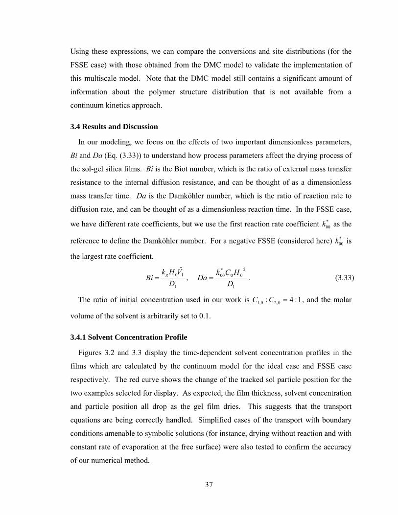
37

Using these expressions, we can compare the conversions and site distributions (for the

FSSE case) with those obtained from the DMC model to validate the implementation of

this multiscale model. Note that the DMC model still contains a significant amount of

information about the polymer structure distribution that is not available from a

continuum kinetics approach.

3.4 Results and Discussion

In our modeling, we focus on the effects of two important dimensionless parameters,

Bi and Da (Eq. (3.33)) to understand how process parameters affect the drying process of

the sol-gel silica films. Bi is the Biot number, which is the ratio of external mass transfer

resistance to the internal diffusion resistance, and can be thought of as a dimensionless

mass transfer time. Da is the Damköhler number, which is the ratio of reaction rate to

diffusion rate, and can be thought of as a dimensionless reaction time. In the FSSE case,

we have different rate coefficients, but we use the first reaction rate coefficient *00k as the

reference to define the Damköhler number. For a negative FSSE (considered here) *00k is

the largest rate coefficient.

1

10ˆ

DVHk

Bi g= , 1

200

*00

DHCk

Da = . (3.33)

The ratio of initial concentration used in our work is 1:4: 0,20,1 =CC , and the molar

volume of the solvent is arbitrarily set to 0.1.

3.4.1 Solvent Concentration Profile

Figures 3.2 and 3.3 display the time-dependent solvent concentration profiles in the

films which are calculated by the continuum model for the ideal case and FSSE case

respectively. The red curve shows the change of the tracked sol particle position for the

two examples selected for display. As expected, the film thickness, solvent concentration

and particle position all drop as the gel film dries. This suggests that the transport

equations are being correctly handled. Simplified cases of the transport with boundary

conditions amenable to symbolic solutions (for instance, drying without reaction and with

constant rate of evaporation at the free surface) were also tested to confirm the accuracy

of our numerical method.

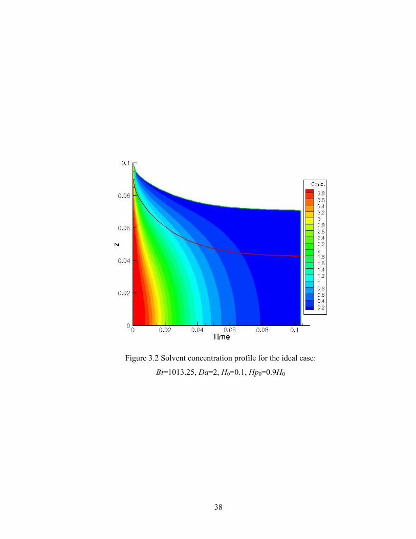
38

Figure 3.2 Solvent concentration profile for the ideal case:

Bi=1013.25, Da=2, H0=0.1, Hp0=0.9H0

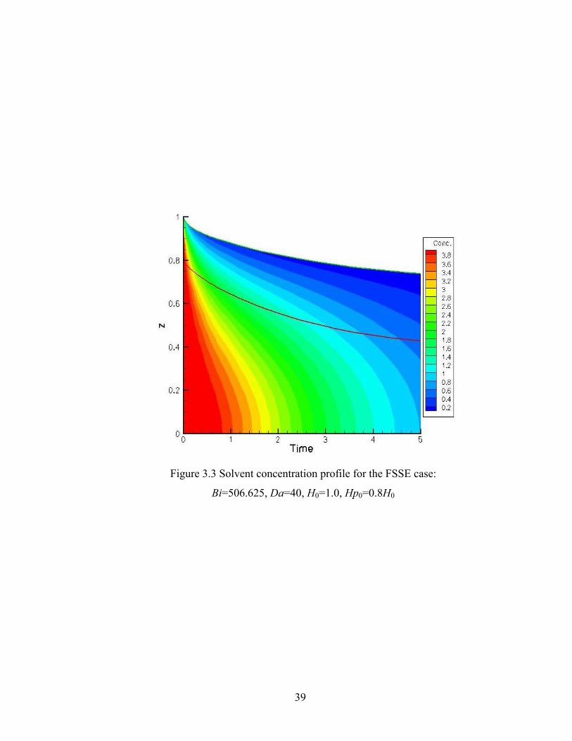
39

Figure 3.3 Solvent concentration profile for the FSSE case:

Bi=506.625, Da=40, H0=1.0, Hp0=0.8H0

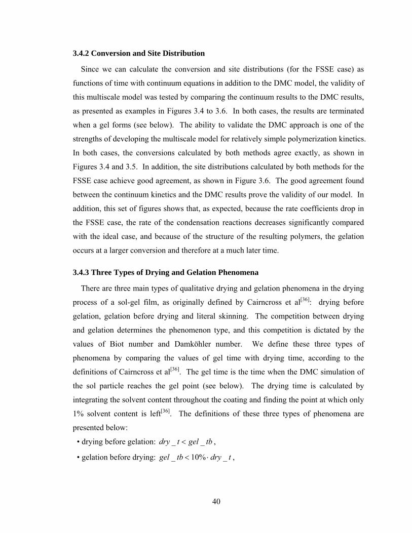
40

3.4.2 Conversion and Site Distribution

Since we can calculate the conversion and site distributions (for the FSSE case) as

functions of time with continuum equations in addition to the DMC model, the validity of

this multiscale model was tested by comparing the continuum results to the DMC results,

as presented as examples in Figures 3.4 to 3.6. In both cases, the results are terminated

when a gel forms (see below). The ability to validate the DMC approach is one of the

strengths of developing the multiscale model for relatively simple polymerization kinetics.

In both cases, the conversions calculated by both methods agree exactly, as shown in

Figures 3.4 and 3.5. In addition, the site distributions calculated by both methods for the

FSSE case achieve good agreement, as shown in Figure 3.6. The good agreement found

between the continuum kinetics and the DMC results prove the validity of our model. In

addition, this set of figures shows that, as expected, because the rate coefficients drop in

the FSSE case, the rate of the condensation reactions decreases significantly compared

with the ideal case, and because of the structure of the resulting polymers, the gelation

occurs at a larger conversion and therefore at a much later time.

3.4.3 Three Types of Drying and Gelation Phenomena

There are three main types of qualitative drying and gelation phenomena in the drying

process of a sol-gel film, as originally defined by Cairncross et al[36]: drying before

gelation, gelation before drying and literal skinning. The competition between drying

and gelation determines the phenomenon type, and this competition is dictated by the

values of Biot number and Damköhler number. We define these three types of

phenomena by comparing the values of gel time with drying time, according to the

definitions of Cairncross et al[36]. The gel time is the time when the DMC simulation of

the sol particle reaches the gel point (see below). The drying time is calculated by

integrating the solvent content throughout the coating and finding the point at which only

1% solvent content is left[36]. The definitions of these three types of phenomena are

presented below:

• drying before gelation: tbgeltdry __ < ,

• gelation before drying: tdrytbgel _%10_ ⋅< ,

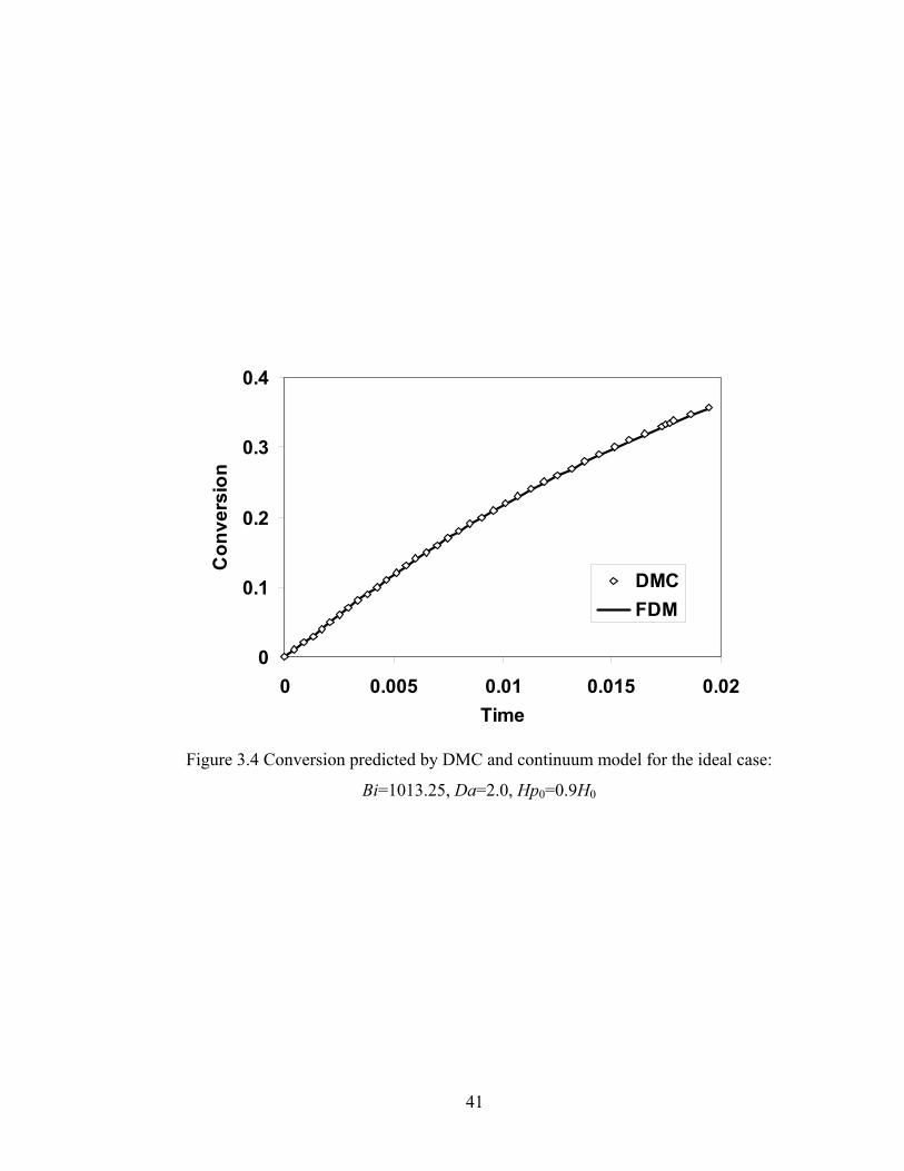
41

0

0.1

0.2

0.3

0.4

0 0.005 0.01 0.015 0.02Time

Con

vers

ion

DMCFDM

Figure 3.4 Conversion predicted by DMC and continuum model for the ideal case:

Bi=1013.25, Da=2.0, Hp0=0.9H0

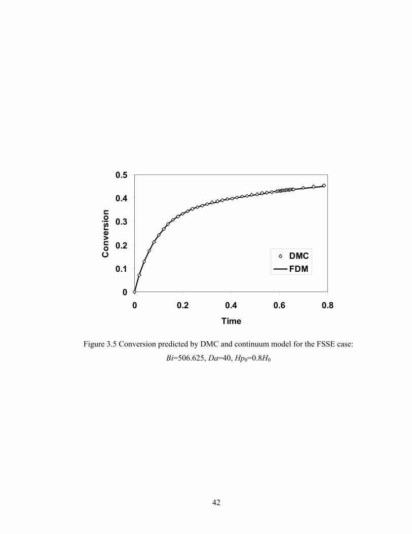
42

0

0.1

0.2

0.3

0.4

0.5

0 0.2 0.4 0.6 0.8

Time

Con

vers

ion

DMCFDM

Figure 3.5 Conversion predicted by DMC and continuum model for the FSSE case:

Bi=506.625, Da=40, Hp0=0.8H0

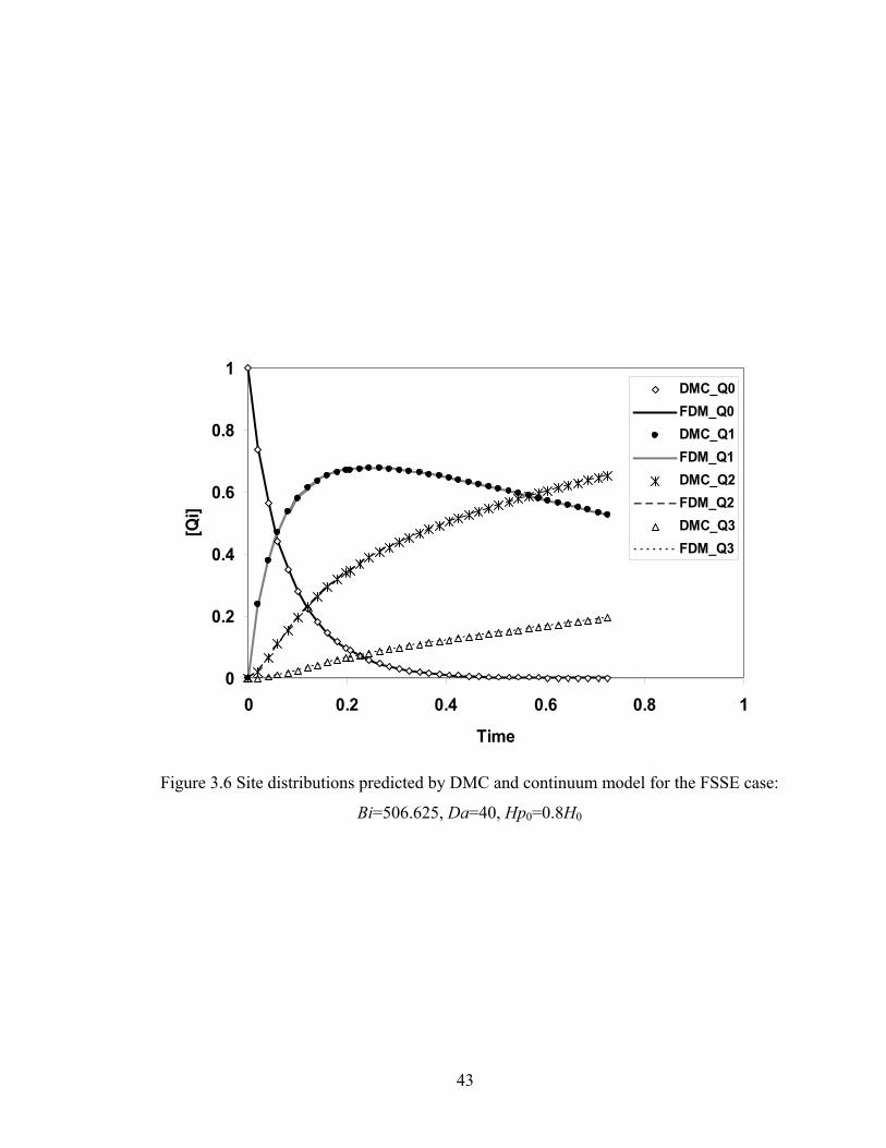
43

0

0.2

0.4

0.6

0.8

1

0 0.2 0.4 0.6 0.8 1

Time

[Qi]

DMC_Q0FDM_Q0DMC_Q1FDM_Q1DMC_Q2FDM_Q2DMC_Q3FDM_Q3

Figure 3.6 Site distributions predicted by DMC and continuum model for the FSSE case:

Bi=506.625, Da=40, Hp0=0.8H0

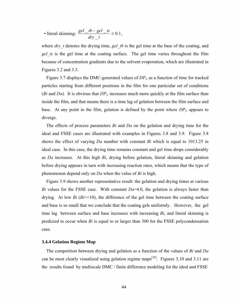
44

• literal skinning: 1.0_

__≥

−tdry

tsgeltbgel ,

where dry_t denotes the drying time, gel_tb is the gel time at the base of the coating, and

gel_ts is the gel time at the coating surface. The gel time varies throughout the film

because of concentration gradients due to the solvent evaporation, which are illustrated in

Figures 3.2 and 3.3.

Figure 3.7 displays the DMC-generated values of DPw as a function of time for tracked

particles starting from different positions in the film for one particular set of conditions

(Bi and Da). It is obvious that DPw increases much more quickly at the film surface than

inside the film, and that means there is a time lag of gelation between the film surface and

base. At any point in the film, gelation is defined by the point where DPw appears to

diverge.

The effects of process parameters Bi and Da on the gelation and drying time for the

ideal and FSSE cases are illustrated with examples in Figures 3.8 and 3.9. Figure 3.8

shows the effect of varying Da number with constant Bi which is equal to 1013.25 in

ideal case. In this case, the drying time remains constant and gel time drops considerably

as Da increases. At this high Bi, drying before gelation, literal skinning and gelation

before drying appears in turn with increasing reaction rates, which means that the type of

phenomenon depend only on Da when the value of Bi is high.

Figure 3.9 shows another representative result: the gelation and drying times at various

Bi values for the FSSE case. With constant Da=4.0, the gelation is always faster than

drying. At low Bi (Bi<=10), the difference of the gel time between the coating surface

and base is so small that we conclude that the coating gels uniformly. However, the gel

time lag between surface and base increases with increasing Bi, and literal skinning is

predicted to occur when Bi is equal to or larger than 300 for the FSSE polycondensation

case.

3.4.4 Gelation Regime Map

The competition between drying and gelation as a function of the values of Bi and Da

can be most clearly visualized using gelation regime maps[36]. Figures 3.10 and 3.11 are

the results found by multiscale DMC / finite difference modeling for the ideal and FSSE

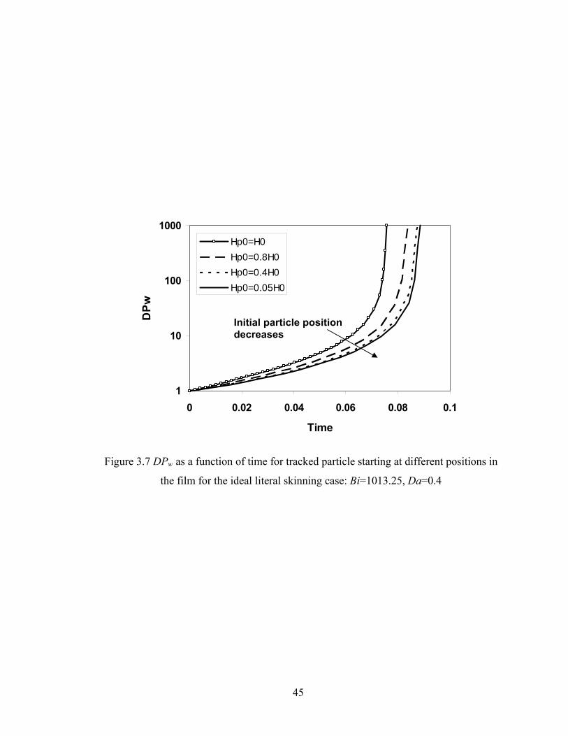
45

Figure 3.7 DPw as a function of time for tracked particle starting at different positions in

the film for the ideal literal skinning case: Bi=1013.25, Da=0.4

1

10

100

1000

0 0.02 0.04 0.06 0.08 0.1

Time

DPw

Hp0=H0Hp0=0.8H0Hp0=0.4H0Hp0=0.05H0

Initial particle position decreases

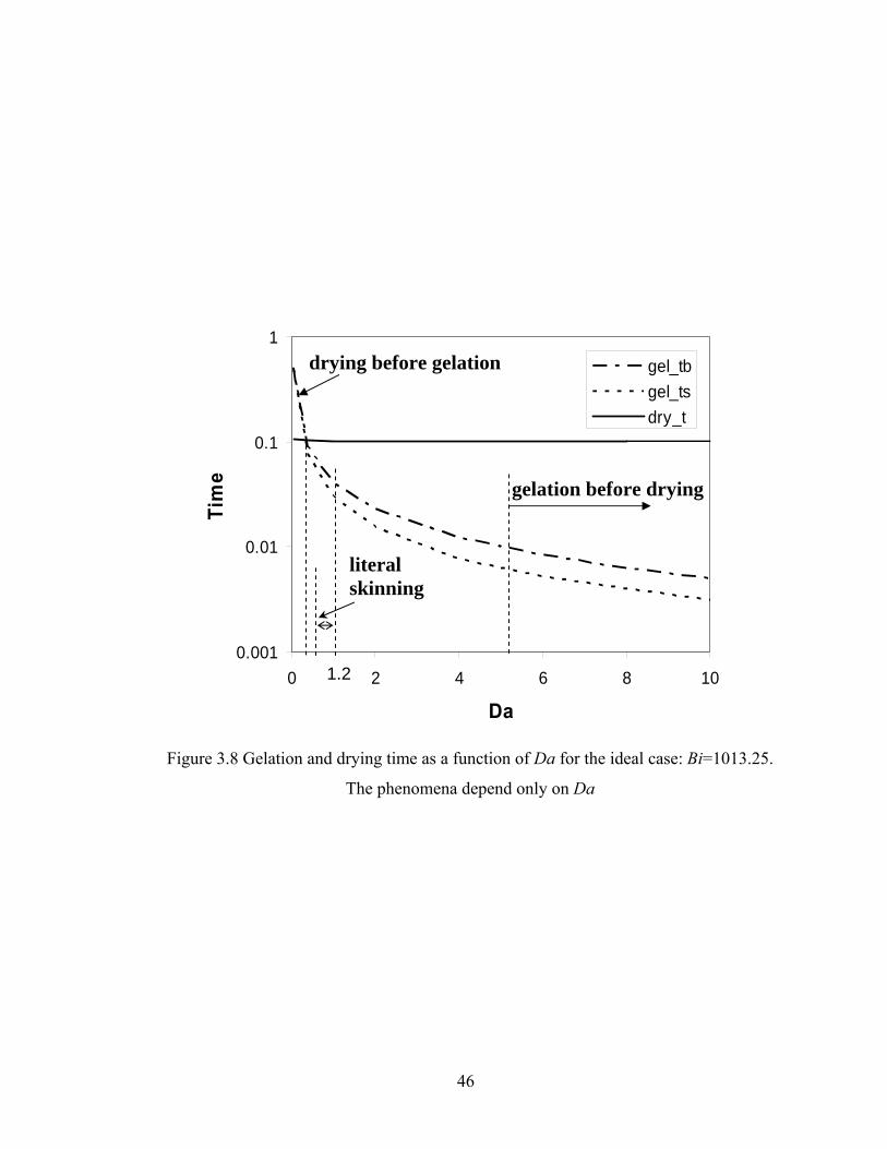
46

Figure 3.8 Gelation and drying time as a function of Da for the ideal case: Bi=1013.25.

The phenomena depend only on Da

0.001

0.01

0.1

1

0 2 4 6 8 10

Da

Tim

e

gel_tbgel_tsdry_t

1.2

literal skinning

gelation before drying

drying before gelation

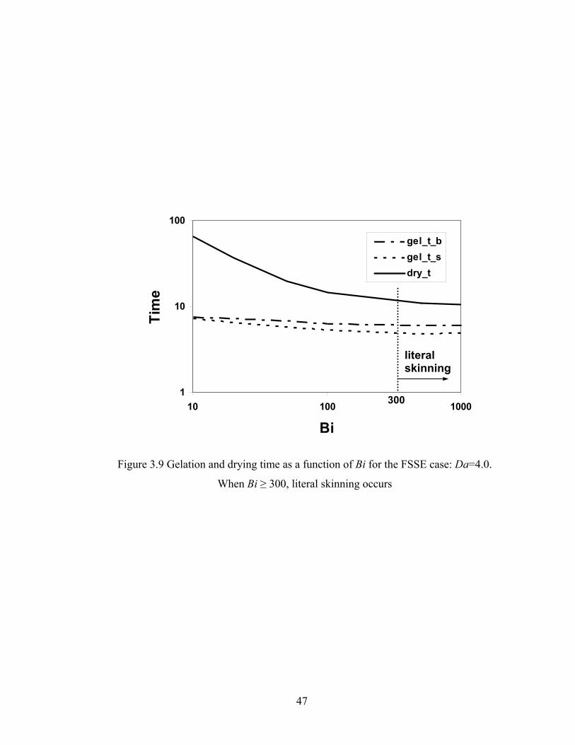
47

Figure 3.9 Gelation and drying time as a function of Bi for the FSSE case: Da=4.0.

When Bi ≥ 300, literal skinning occurs

1

10

100

10 100 1000

Bi

Tim

e

gel_t_bgel_t_sdry_t

literal skinning

300

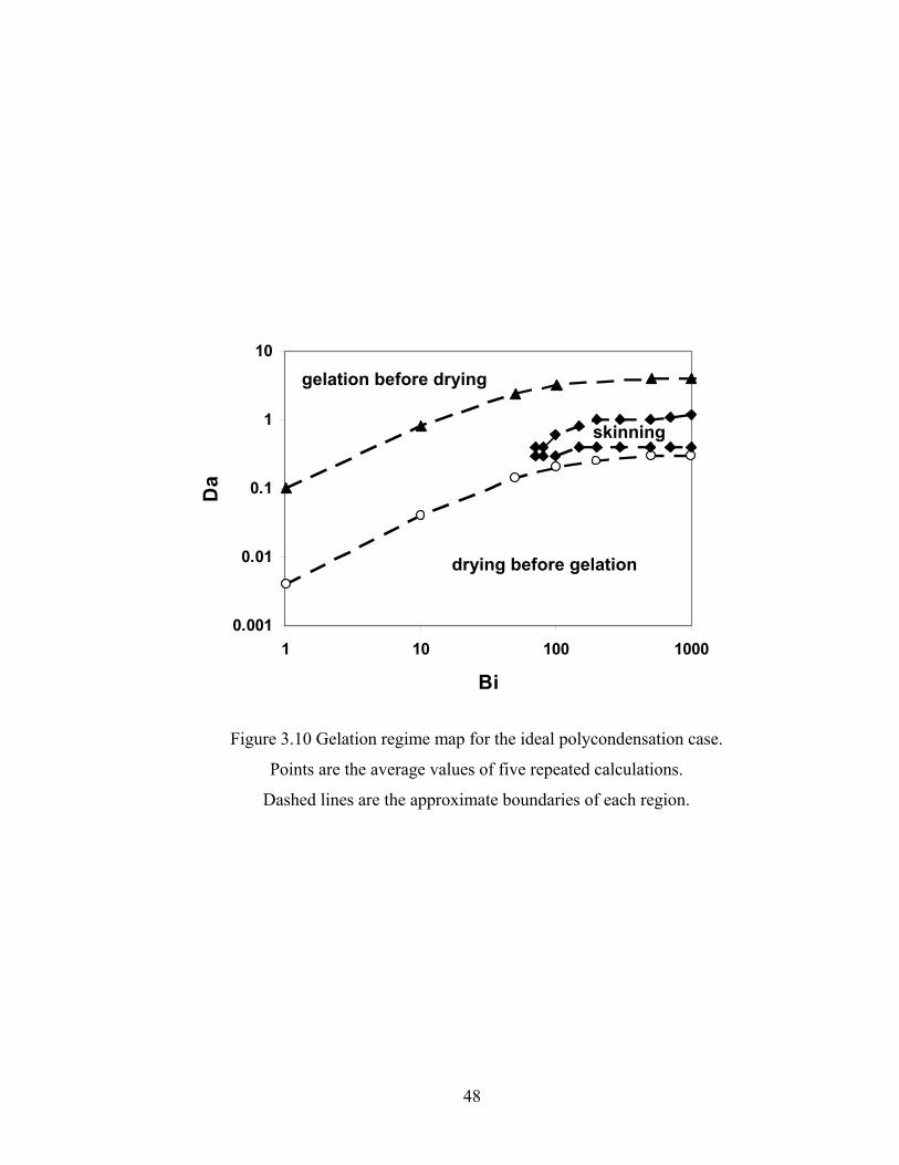
48

Figure 3.10 Gelation regime map for the ideal polycondensation case.

Points are the average values of five repeated calculations.

Dashed lines are the approximate boundaries of each region.

0.001

0.01

0.1

1

10

1 10 100 1000

Bi

Da



skinning

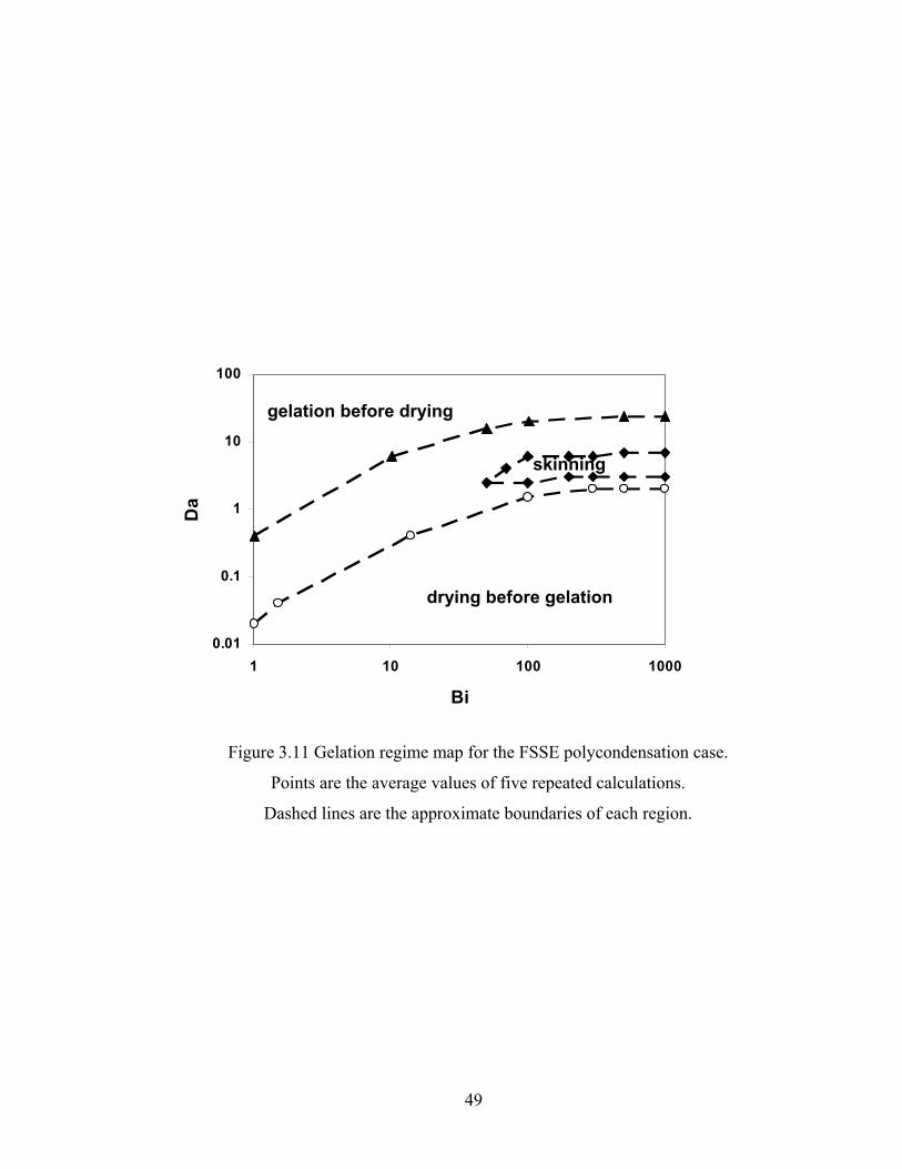
49

Figure 3.11 Gelation regime map for the FSSE polycondensation case.



0.01

0.1

1

10

100

1 10 100 1000

Bi

Da



skinning

50

cases, respectively. The lines are the approximate boundaries between regions (as

defined above) and the points are the conditions related to each phenomenon[36], which

are the average values of five repeated simulations. At low Da, the coating dries before it

gels and at high Da, the gelation reaction rates are much quicker than the drying rate.

With high Bi, literal skinning occurs between the regions of “drying before gelation” and

“gelation before drying”. The maps are similar for the ideal and FSSE cases, except that

with FSSE, all three regions are shifted towards higher Da. These results are consistent

with the findings of Cairncross et al.[36], but they used an approximate kinetic-recursive

model with reduced accuracy for FSSE modeling and which is not capable of correctly

modeling the high degree of cyclization found in real sol-gel polymerization (to be

discussed in Chapter 4 and 5).

3.4.5 Relationship between Gel Time and Initial Particle Position

To gain more insight into the effects of the FSSE on film uniformity, we further

investigate the relationship between gel time and initial particle position for the three

types of phenomena, as shown in Figures 3.12 and 3.13. Representative points from the

gelation regime maps are shown. According to the maps, we can observe all three types

of phenomena by setting Bi to a high value and varying Da. In order to compare these

three types phenomena easily, all of the gel time values are normalized by the one at the

surface. With fixed Bi, gel times are, of course, longest when “drying before gelation” is

found and smallest when “gelation before drying” is found. The gel time gradient is

much more severe when “gelation before drying” is observed than with “drying before

gelation”. This suggests that, when the coating dries completely as a liquid (drying

before gelation) the gel time lag is small and defects are not likely to appear due to

formation of a gel layer at the film surface, and when the coating gels before it is dry, the

difference of gel time is more visible and likely to induce defects. Regardless of the rate

of drying, drying before gelation is best achieved by reducing the rate of condensation

relative to the rate of diffusion of solvent. In sol-gel systems, this is best accomplished by

working near the minimum condensation rate which occurs at a pH of ~2. Gel times for

the FSSE case simulations are longer than those of ideal case, proving again that gelation

is delayed compared with the ideal case, as we mentioned earlier. Also, the gradients in

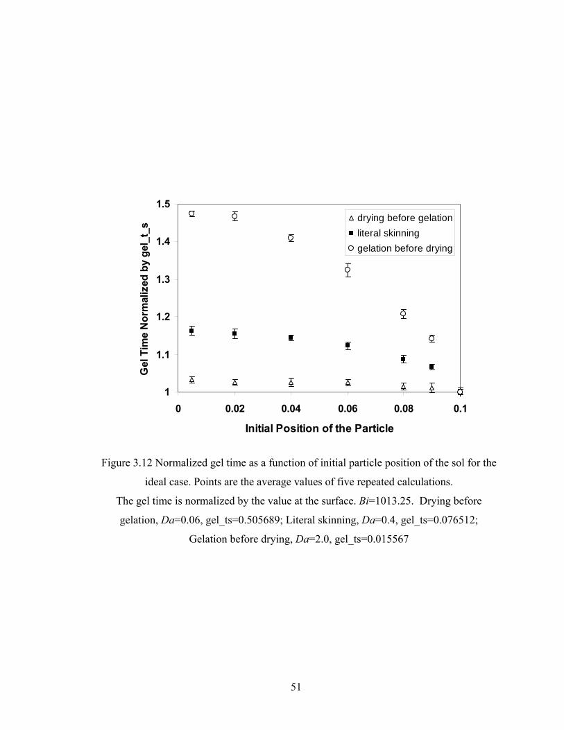
51

1

1.1

1.2

1.3

1.4

1.5

0 0.02 0.04 0.06 0.08 0.1

Initial Position of the Particle

Gel

Tim

e N

orm

aliz

ed b

y ge

l_t_

s drying before gelationliteral skinninggelation before drying

Figure 3.12 Normalized gel time as a function of initial particle position of the sol for the

ideal case. Points are the average values of five repeated calculations.

The gel time is normalized by the value at the surface. Bi=1013.25. Drying before

gelation, Da=0.06, gel_ts=0.505689; Literal skinning, Da=0.4, gel_ts=0.076512;

Gelation before drying, Da=2.0, gel_ts=0.015567

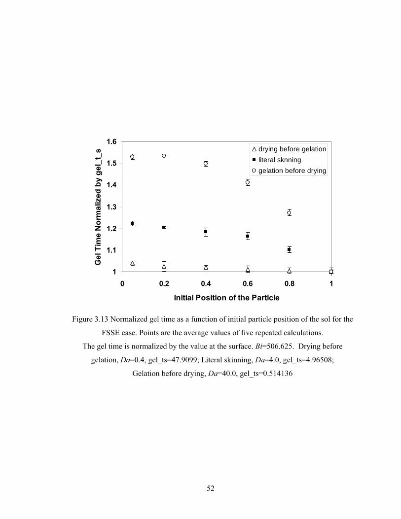
52

1

1.1

1.2

1.3

1.4

1.5

1.6

0 0.2 0.4 0.6 0.8 1

Initial Position of the Particle

Gel

Tim

e N

orm

aliz

ed b

y ge

l_t_

s drying before gelationliteral sknninggelation before drying

Figure 3.13 Normalized gel time as a function of initial particle position of the sol for the

FSSE case. Points are the average values of five repeated calculations.

The gel time is normalized by the value at the surface. Bi=506.625. Drying before

gelation, Da=0.4, gel_ts=47.9099; Literal skinning, Da=4.0, gel_ts=4.96508;

Gelation before drying, Da=40.0, gel_ts=0.514136

53

gel time are more severe than those found in the ideal case, suggesting that nonideal

polymerization may worsen the formation of coating defects in sol-gel systems.

3.5 Summary

The proposed multiscale model for the drying process of sol-gel coatings couples

molecular to macroscopic phenomena by combining dynamic Monte Carlo simulations

and the finite difference method. For the cases studied here, continuum equations can be

formulated for the overall extent of reaction, and the results agree well with the

multiscale DMC / FDM model, which demonstrates the validity of the multiscale model.

In the continuum model, the entire DMC simulation is treated as a particle of sol whose

position and composition are tracked using a diffusion / evaporation finite difference

calculation. Therefore, the total silicon concentration, which is provided by the

continuum model, serves as one “handshake” with the DMC model. The second

“handshake” between the models is the time interval from the DMC simulation, which is

used as the time interval for the continuum model. By simulating swarms of particles

starting from different positions in the film and varying process parameters, we observe

their effects on the competition between drying and gelation, predict different drying /

gelation phenomena, and predict the occurrence of gradients of concentration and

gelation in the films which can lead to the formation of a gel skin near the top surface of

the film.

This multiscale model is our first step to understand the drying process of sol-gel

coating. Further efforts are needed to improve the realism of the polymerization model,

the most important and obvious of which is to add the cyclization in the model and see its

effects on gelation regime maps and structural gradients. We expect that the results of

our simulation will allow better prediction of the formation of structure gradients in sol-

gel derived ceramics and other nonideal multifunctional polycondensation products, and

that this will help in developing coating procedures to reduce coating defects.

54

Chapter 4

Multiscale Modeling with Unlimited 3-membered Ring Cyclization

4.1 Introduction

The coating process of sol-gel films involves multiple length and time scales ranging

from molecular to macroscopic. At the molecular scale, polymerization and (with

surfactant templates) self-assembly processes occur which control the film properties

such as film microstructure. At the same time, macroscopic parameters control the

formation of the film; diffusion and mass transport occur over micron or greater length

scale, and define the concentration fields within which polymerization and self-assembly

occur. Therefore, a multiscale model should be used to link these different length and

time scale together. In our previous chapter, we developed a multiscale model to describe

the competition between polymerization reaction and mass transfer, but we didn’t include

cyclization in our model. However, experiments have shown that three- and four-

membered rings exist early in alkoxysilane polymerization processes and give rise to a

gel conversion as large as 82%[27, 41, 43, 47, 66]. Researchers have also presented several

probable reasons for the occurrence of cyclization. West and coworkers[40] presented

quantum chemical calculations indicating that cycles are energetically favored over

chains extension. Tang et al.[41] proposed that ring formation is easy because of the

flexibility of siloxane chains, and as a unimolecular reaction, cyclization is favored by a

low concentration of monomer. Both Sanchez et al.[42] and Ng et al.[52] presented

evidence that kinetic trends may favor cyclization of silanes. Ng et al.[52] also proposed

that stabilization of rings toward solvent attack or changes in functional group reactivity

favor cyclization. Hence, cyclization is very important at the molecular scale of sol-gel

drying process so that it can’t be neglected at all. Models without cyclization may be

able to match the kinetics of polymerization but they may not be able to correctly model

large-scale (gel) structures, may include wrong parameters and may give incorrect

prediction of the effects of process parameters. Therefore, a better multiscale model for

silica should also include cyclization in the polymerization process.

55

Some researchers have already tried to include the cyclization effect in their models of

sol-gel polymerization, but they often include simplifications that limit their fidelity. For

instance, Vainrub et al.[44] didn’t directly simulate cyclization in their kinetic model.

Instead, they used rate coefficients whose values decreased as a function of time to mimic

the kinetic effect of cyclization. Hendrickson et al.[65] also simulated cyclization during

stepwise polymerization. They assumed that each monomer was a stationary hard sphere,

and reactions were only allowed to happen when two randomly chosen monomers were

within a sphere of radius rh which was centered on one of the reactants. While they

admitted that this method had shortcoming that real diffusion of monomers was not

modeled, this approach did capture the effect of cyclization on delaying gelation to some

extent. Kasehagen et al.[39] limited their simulation of cyclization to include only

cyclization of trimers and linear tetramers. Rankin et al.[27] also used this kinetics of

forming single rings as a first step to model the cyclization effect in polymerizing silane

solutions. Ng et al. [43] treated cyclic or even cagelike intermediates as f-functional

random branching “monomeric” units (i.e. new precursors). These cyclic (cagelike)

intermediates were assumed to form in the early stage of reactions from monomers by

cyclization, but after they were formed, they could only connect with each other until

forming a gel. Highly cyclized cages were shown to give a gelation conversion close to

the experimental value. Rankin et al.[38] first presented a model with extensive

cyclization to form polycyclic structures made up of three-membered rings. They applied

the dynamic Monte Carlo (DMC) simulation technique which has advantages over

statistical approaches due to full accounting of the reaction history, molecular structure

and weight distributions, membership in cyclic and polycyclic species, and so on.

Similar to the work of Rankin et al, here we add unlimited cyclization to form only three-

membered rings in our multiscale model of sol-gel silica drying films. This is our first

step to investigate how extensive cyclization affects the sol-gel process in a drying film.

More details will be given below.

56

4.2 DMC Model

In this chapter, we will describe our DMC modeling approach and give details about

new approaches used to track the effects of cyclization, e.g. calculating the Wiener index,

a topological index related to molecular size.

4.2.1 Bimolecular Condensation

Experiments have shown that under acid-catalyzed conditions, the hydrolysis reaction

of alkoxysilanes reaches pseudoequilibrium[28]. This often results in a constant average

extent of hydrolysis χ , which is defined as:

][][

][SiORSiOH

SiOH+

=χ . (4.1)

By assuming that water-producing condensation dominates over alcohol-producing

condensation[37], and based on the fact that a strong, negative first shell substitution effect

(FSSE) exists in the condensation reactions[30], the set of bimolecular condensation

reactions among silicon sites can be written as[38]:

OHQQQQ jik

jiij

211 ++⎯→⎯+ ++ , =ji, 0, 1, 2, 3 (4.2)

where Qi represents a tetrafunctional silicon site with i siloxane bonds. With these

assumptions, the bimolecular rate expressions are given by [38]:

⎪⎩

⎪⎨⎧

=−−

≠−−=

jiQQjfifk

jiQQjfifkR

jiij


21

],][)[)((*

*

(4.3)

Where ijij kχk 2* = and f = the functionality of the monomer (f = 4 for tetrafunctional

silane precursors). The matrix of rate coefficients is set to mimic the experimental trend

observed for alkoxysilanes under acidic conditions[39]:

K*

⎥⎥⎥⎥

⎦

⎤

⎢⎢⎢⎢

⎣

⎡

=

001.0009.001.0081.009.01.0729.081.09.00.1

*00k

57

4.2.2 Three-membered Ring Cyclization

After some reaction steps, oligomers of size large enough to form rings will have

formed. Cyclization reactions can then occur when two sites chosen to react are in the

same molecule. This results in a new ring within an existing molecule. According to the

approach of Rankin et al.[38], we use bond blocks ijn B to calculate the cyclization rates.

Here the superscript n represents the number of bonds between two sites, and subscripts i

and j represent the connectivities of the ends (i.e. the number of siloxane bonds attached

to each end). For example, a linear trimer has one 112B bond block, while a linear

tetramer has two 122B blocks and one 11

3B block. As the first step in our multiscale

model with cyclization, we just consider the formation of three-membered rings.

Therefore we just need to pay attention to two-bond blocks. In this case, the rate of

cyclization reactions is calculated by analogy with any isolated ring closure reaction as[38]:

][))(( 2*),(3

3ijjic

cycij BkjfifR −−= , =ji & 1, 2, 3. (4.4)

In order to have the concentrations of these two-bond blocks, the number of ijB2 of

each type needs to be updated after each reaction step, by adding the new bond blocks

created by the reaction and modifying the old ones that have changed. Figure 4.1 shows

an example of a new ring formed in an existing molecule. From this example, we can see

that after each cyclization reaction, only the first- and second- shell neighbors of the

reacting sites are involved in changes of ijB2 blocks. Therefore, updating the list of ijB2

sites is accomplished with a set of subroutines that enumerate all first and second shell

neighbors of a pair of reacting sites and test for changes, not considering neighbors

outside the second shell, thus avoiding over-counting of new blocks.

We assume that the substitution effect for cyclization reactions follows the same trend

as for bimolecular reactions, since it still involves nucleophilic displacement between

sites of varying connectivity:

⎥⎥⎥

⎦

⎤

⎢⎢⎢

⎣

⎡=

01.009.01.081.09.00.1

*)1,1(3

*3 cc kK .

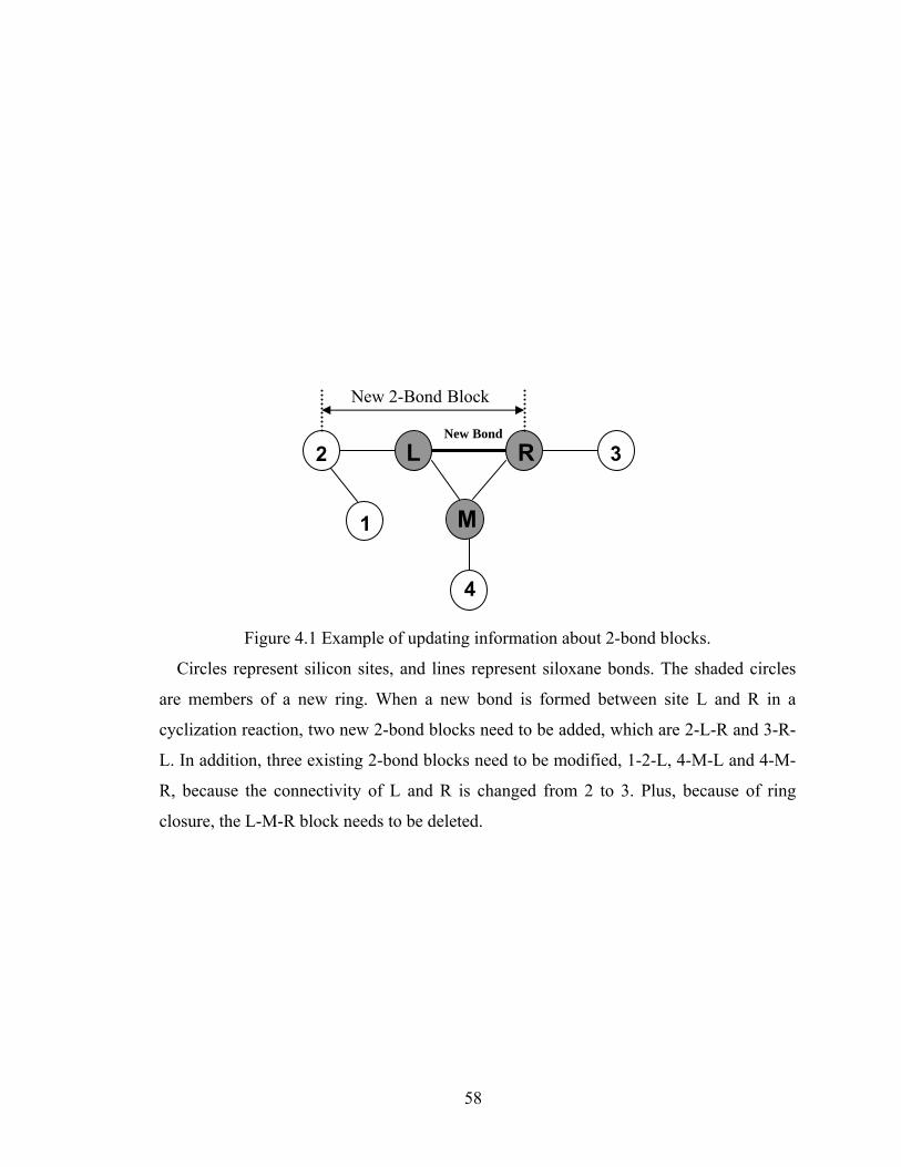
58

Figure 4.1 Example of updating information about 2-bond blocks.

Circles represent silicon sites, and lines represent siloxane bonds. The shaded circles

are members of a new ring. When a new bond is formed between site L and R in a

cyclization reaction, two new 2-bond blocks need to be added, which are 2-L-R and 3-R-

L. In addition, three existing 2-bond blocks need to be modified, 1-2-L, 4-M-L and 4-M-

R, because the connectivity of L and R is changed from 2 to 3. Plus, because of ring

closure, the L-M-R block needs to be deleted.

New Bond

M

L R

New 2-Bond Block

2

1

3

4

59

To characterize the cyclization tendency, the dimensionless parameter κ is used as

defined by Rankin et al.[38]:

0

*11

*)1,1(3

][Sikk

κ c≡ . (4.5)

4.2.3 Wiener Index

In our multiscale model, we record a new type of information (relative to prior DMC

studies) which can be used to characterize molecular size and shape – the Wiener index.

The Wiener index is a topological index that has been shown to be proportional to zero-

shear viscosity, and thus to relate molecular structure and rheology[90]. It is defined as

follows[91]:

∑∑≤

==ji

ijji

ij ddW,2

1 , (4.6)

where ijd is the topological distance (i.e. number of bonds along the shortest path

connected by bonds) between sites i and j in the molecule. Because the Wiener index

takes into account the distribution of topological distances between sites in a molecule, it

can be used as a measure of molecular compactness. It can also be used in quantitative

structure activity/property relationship (QSAR/QSPR) modeling in chemistry[92, 93], for

example, by using Wiener index in QSPR to model the boiling temperature, molar heat

capacity, standard Gibbs energy of formation, vaporization enthalpy, refractive index,

and density of alkanes[93].

If the molecules are linear, the Wiener index can be easily calculated according to the

following expression[91, 94]:

)1(61 2 −= mmWlin , (4.7)

where m is the degree of polymerization. However, calculations of the Wiener index of

arbitrarily branched and cyclic molecules are much more complicated. Here we present a

new algorithm to calculate the Wiener index during dynamic Monte Carlo simulation of

polycondensation. In our model, the sites are silicon atoms, and the bonds are not single

bonds but Si-O-Si bonds. At first, the Wiener index for all monomers is 0. After each

reaction (bimolecular or cyclization reaction), we calculate the Wiener index of the

60

product based on the known indices of the reactant molecule(s) and the distances from

the reacting sites to all other sites.

For bimolecular polycondensation, we assume that the reaction occurs between two

molecules of sizes m and n, to produce a new molecule of size (m+n). Because the

adjacency matrix has not changed in either of the blocks taken from the old molecules,

the distance matrix also will not have changed in each of those blocks from what it was in

the old molecule (Figure 4.2). Therefore, we only need to calculate the distance sub-

matrix for the new nm× section of the distance matrix. The Wiener index of the new

molecule therefore is composed of three parts:

newBA WWWW ++= , (4.8)

where WA and WB are the Wiener indices of the reactant molecules A and B, and Wnew is

the index calculated using only the new nm× submatrix.

Noting that any new pathway between a site in submolecule A and a site in

submolecule B must pass through the new bond between them, the new distance can be

expressed in terms of its distance to the sites at new bond. For example, in Figure 4.3,

1−+= LjiRij ddd (4.9)

When this expression is inserted into the definition of the Wiener index of the new

submatrix, the calculation becomes simple:

∑∑∑∑= == =

−+==m

i

n

jLjiR

m

i

n

jijnew dddW

1 11 1)1( (4.10)

mndmdnn

jLj

m

iiR −+= ∑∑

== 11

In our model, the whole submolecule A is traversed starting from site L to calculate the

distance from each site in submolecule A to site R. A similar procedure is done for

submolecule B. The advantage of this approach is that the calculation of the Wiener

index for the new molecule scales linearly with (m+n). Competing algorithms based on

brute-force calculation of the distance matrix[95, 96] would scale much more poorly with

molecule size.

The Wiener indices of linear molecules with the same degrees of polymerization as the

actual simulated molecules are also tracked in our model for comparison purpose, and the

new piece of the Wiener index due to a bimolecular reaction is given by:

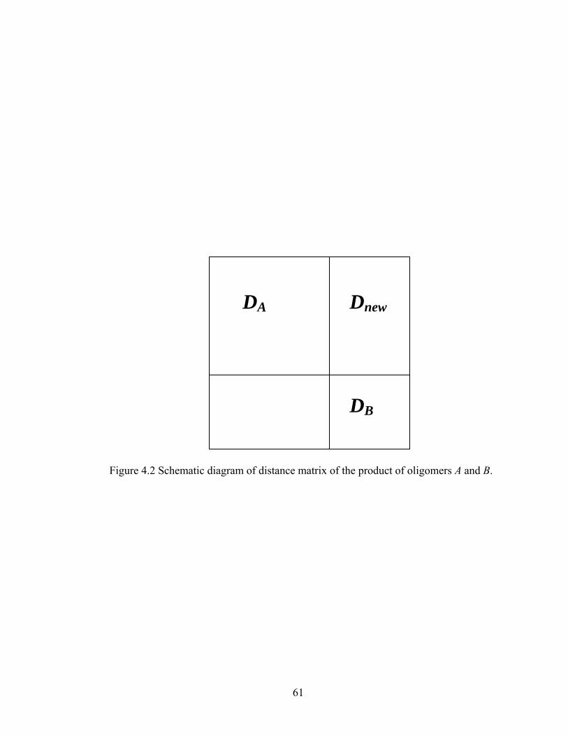
61

Figure 4.2 Schematic diagram of distance matrix of the product of oligomers A and B.

DA

DB

Dnew

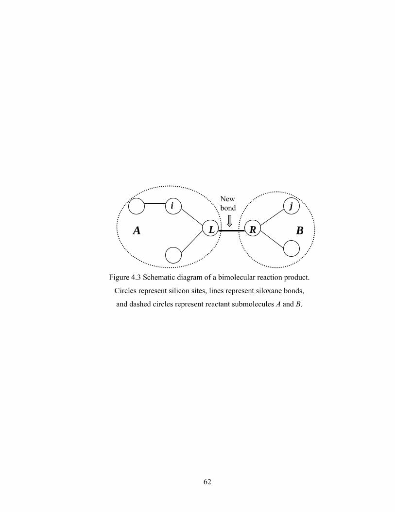
62

Figure 4.3 Schematic diagram of a bimolecular reaction product.

Circles represent silicon sites, lines represent siloxane bonds,

and dashed circles represent reactant submolecules A and B.

L R

New bond

A B

j i

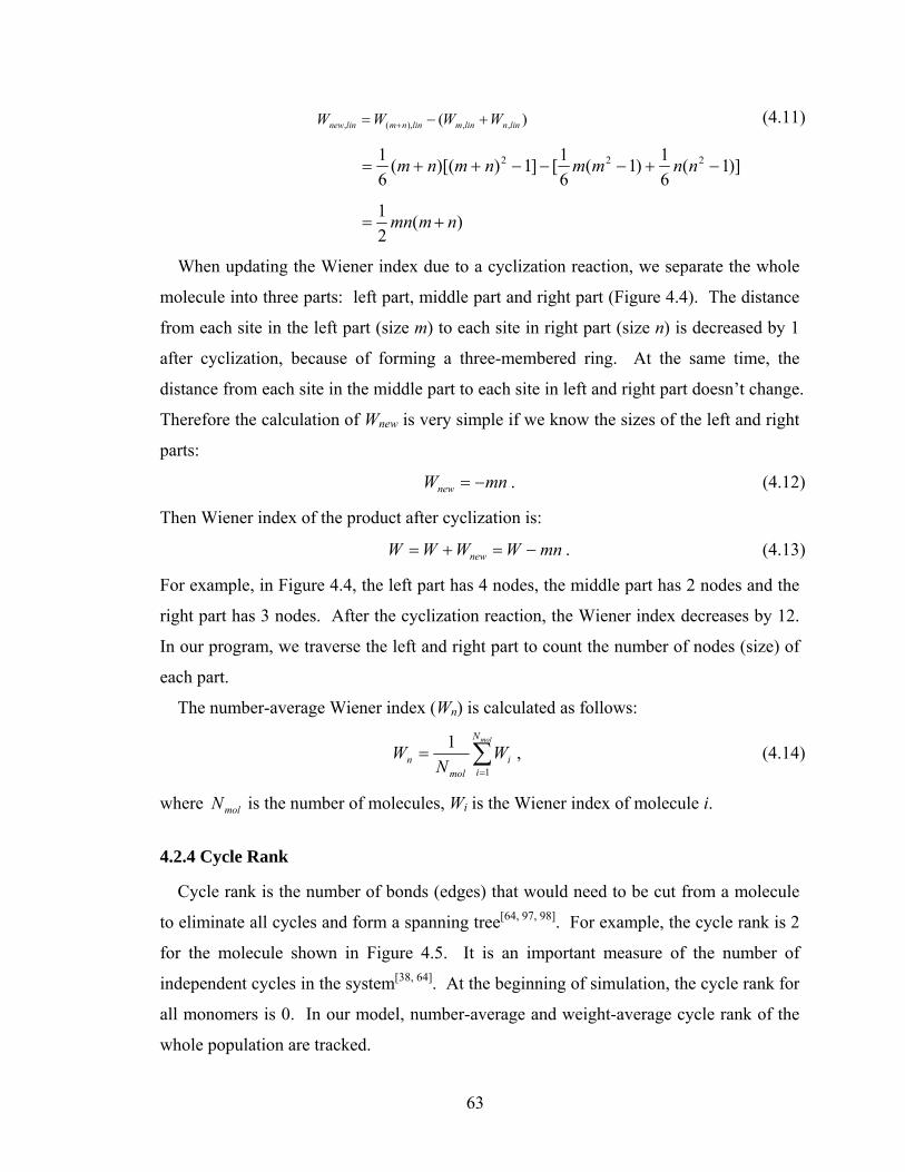
63

)( ,,),(, linnlinmlinnmlinnew WWWW +−= + (4.11)

)]1(61)1(

61[]1))[((

61 222 −+−−−++= nnmmnmnm

)(21 nmmn +=

When updating the Wiener index due to a cyclization reaction, we separate the whole

molecule into three parts: left part, middle part and right part (Figure 4.4). The distance

from each site in the left part (size m) to each site in right part (size n) is decreased by 1

after cyclization, because of forming a three-membered ring. At the same time, the

distance from each site in the middle part to each site in left and right part doesn’t change.

Therefore the calculation of Wnew is very simple if we know the sizes of the left and right

parts:

mnWnew −= . (4.12)

Then Wiener index of the product after cyclization is:

mnWWWW new −=+= . (4.13)

For example, in Figure 4.4, the left part has 4 nodes, the middle part has 2 nodes and the

right part has 3 nodes. After the cyclization reaction, the Wiener index decreases by 12.

In our program, we traverse the left and right part to count the number of nodes (size) of

each part.

The number-average Wiener index (Wn) is calculated as follows:

∑=

=molN

ii

moln W

NW

1

1 , (4.14)

where molN is the number of molecules, Wi is the Wiener index of molecule i.

4.2.4 Cycle Rank

Cycle rank is the number of bonds (edges) that would need to be cut from a molecule

to eliminate all cycles and form a spanning tree[64, 97, 98]. For example, the cycle rank is 2

for the molecule shown in Figure 4.5. It is an important measure of the number of

independent cycles in the system[38, 64]. At the beginning of simulation, the cycle rank for

all monomers is 0. In our model, number-average and weight-average cycle rank of the

whole population are tracked.

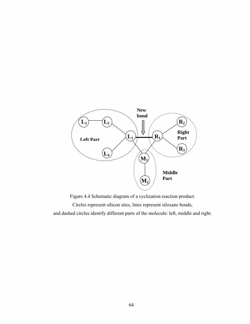
64

Figure 4.4 Schematic diagram of a cyclization reaction product.

Circles represent silicon sites, lines represent siloxane bonds,

and dashed circles identify different parts of the molecule: left, middle and right.

L1

L2 L3

L4

R1

R2

R3

M1

M2

Right Part Left Part

Middle Part

New bond

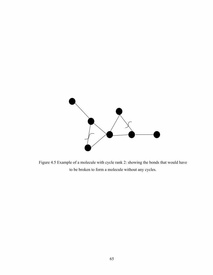
65

Figure 4.5 Example of a molecule with cycle rank 2: showing the bonds that would have

to be broken to form a molecule without any cycles.

66

∑=

=molN

ii

moln Cr

NCr

1

1 , )(11∑=

⋅=molN

iiiw DPCr

NCr , (4.15)

where Cri is the cycle rank of molecule i, DPi is the degree of polymerization of molecule

i, and N is the total number of sites (monomers).

4.2.5 Ring Involvement

Ring involvement can be quantified by the average number of independent rings in

which a randomly chosen site is involved[38]. Ring involvement provides additional

insight into the local network structure because it ranges from 0 (no rings) to almost 3

(100% cages for 3-membered rings).

Ring involvement is 0 at the beginning of simulation. Since one new independent ring

is formed after each cyclization reaction, and each ring has three sites, ring involvement

(I) is increased by

N

I 3Δ = . (4.16)

4.2.6 DMC Algorithm

The dynamic Monte Carlo simulation starts with a finite set of N (which is equal to 106

in our model) monomers. The data structures are almost the same compared with our

description of the ideal case in Chapter 2. However, we add arrays to store information

about the distribution of cycle ranks, Wiener indices and the populations of two-bond

blocks. In addition, to allow fast selection of sites for cyclization, we maintain six linked

lists of specific two-bond blocks differentiated by end-site connectivities. The simulation

procedures are the same as other DMC simulations of polycondensation[38, 39]. At each

MC step, a new siloxane bond is formed, and the conversion is increased by a small

constant value (which is 5×10-7 in our model). The time increment is given by[70]:

( )

∑ +⎟⎠⎞⎜

⎝⎛

=)(

1lnΔ

3 cycij

bimolij

SiRRC

Nrt , (4.17)

where N is the total number of sites, r is a random number selected from (0, 1), and bimolijR

and cycijR3 are the rates described by Eq. (4.3) and (4.4). CSi is the total silicon site

67

concentration which comes from the continuum model results (see below). Based on the

three-membered cyclization reaction rates, Monte Carlo reaction selection is performed

in each step to choose the type of reaction to occur. The probability of choosing each

reaction is set equal to its rate over the sum of the rates of all possible reactions. If

cyclization is chosen, we randomly select one two-bond block from the corresponding

linked list. For bimolecular reactions, the reactants are randomly selected from a list

containing all sites grouped according to connectivity. Then we update all the data

structures including the two-bond block information, molecular weight, Wiener index,

cycle rank, and so on. The expressions for the increments of all variables after a DMC

step except for conversion and time are shown in Table 4.1. (The derivations of these

expressions are shown in the Appendix A.)

Using DMC simulation, we are able to keep track of lists of specific two-bond blocks

and then use these to calculate the cyclization rate. This is a significant advantage of the

DMC method compared with statistical models. When nonrandom polymerization

occurs with extensive cyclization, ijB2 populations cannot be correctly predicted by

statistical means. Also with the DMC method, we can obtain gel point information,

molecular weight distribution, Wiener index, and so on, which are related to film

microstructure.


4.3.1 Model Description

The continuum model for the formation of a sol-gel silica coating is described by

macroscopic mass conservation equations. The coating is described here with a

simplified one-dimensional model. Solvent is removed via evaporation continuously at

the top liquid / vapor interface. In addition to evaporation, the diffusion process of

solvent within the film should be taken into account in this model. The assumptions

made in the model are the same as in our previous chapter. The entire DMC simulation

(containing ~ 106 monomers) is treated as a particle of sol whose position and

composition are tracked in the continuum model.

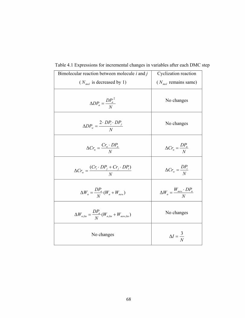
68

Table 4.1 Expressions for incremental changes in variables after each DMC step

Bimolecular reaction between molecule i and j

( molN is decreased by 1)

Cyclization reaction

( molN remains same)

NDPDP n

n

2

Δ =

No changes

NDPDP

DP jiw

⋅⋅=

2Δ

No changes

NDPCrCr nn

n⋅

=Δ

NDPCr n

n =Δ

NDPCrDPCr

Cr ijjiw

)(Δ

⋅+⋅=

NDPCr i

w =Δ

)(Δ newnn

n WWN

DPW +=

NDPWW nnew

n⋅

=Δ

)(Δ ,,, linnewlinnn

linn WWN

DPW +=

No changes

No changes

NI 3Δ =

69

4.3.2 Governing Equations

Since the validity of our multiscale model without cyclization has been verified in

Chapter 3, we can simplify the continuum model to just consider the solvent and total

silica, without including equations for each Qi reactant species.

Therefore, the governing equations are as follows: 2

1 11 2 0C CD

t z∂ ∂

− =∂ ∂

(4.18)

22 2

2 2 0C CDt z

∂ ∂− =

∂ ∂ (4.19)

where C1 is the concentration of solvent, C2 is the total silicon concentration.

The initial conditions are:

( ) 0,11 ,0 CzC = ; ( ) 0,22 ,0 CzC = ; (4.20)

and the boundary conditions are:

At the substrate ( 0=z ): 0=∂∂

zCD i

i ( =i 1, 2); (4.21)

At the free surface ( )(tHz = ): 11 1 1 1

( ) ( )sg

C dH tD C k y yz dt

∞∂− − = −

∂ (4.22)

z

CVV

zC

∂∂

−=∂∂ 1

2

12

ˆˆ

(4.23)

where gk is the mass transfer coefficient of solvent (in units of )/( 2 scmmol ⋅ ), 1sy is the

molar fraction of solvent at the surface in the gas phase (which is calculated based on

Raoult’s law), and 1y∞ is the molar fraction of solvent far away in the gas, which is set to

zero in this paper. As we mentioned in Chapter 3, 0,2

10,12

ˆ1ˆC

VCV

−= , where iV is the molar

volume of component i. Assuming that only solvent evaporates, the rate of change of film

thickness, or surface velocity, can be calculated according to the following expression:

1 1 1( ) ˆ ( )s s

gdH t v V k y y

dt∞= = − − , (4.24)

70


The following dimensionless variables are utilized to solve the governing equations

numerically:

)(/ tHzη = , 0/)( HtHh = , 0/ CCc ii = , tHDτ 2

1= . (4.25)

Using the dimensionless variableη , the new region is always from 0=η to 1=η , that is,

the physically moving domain is mapped onto a fixed domain, and we do not need to

modify the spatial grid during the simulation. The solvent transport equation in

dimensionless form was given in Chapter 3.

This set of dimensionless equations is numerically solved using an explicit centered

finite difference method. We discretize the whole domain into a number of thin slices,

each one with a fixed thickness ηΔ . The time interval tΔ comes from the DMC

simulation, as given by Eq. (4.17) for each DMC step. At the surface, the mole fraction

of solvent in solution is ss

s

cccxm

21

1

+= , s

ic is the dimensionless concentration at the

surface of the solution. Therefore we can calculate the mole fraction of solvent at the

surface in the gas phase using Raoult’s law, t

s

PxmPy ⋅

= 11 , where P1 is the solvent vapor

pressure and Pt is the total pressure. At each finite difference step, we use the

concentrations, film thickness, surface velocity, and Robin boundary conditions at the

surface from the previous time step to complete the calculation. Also, the entire DMC

simulation is treated as a particle of sol whose position and composition are tracked in the

continuum model. We use linear interpolation to perform the tracking of the particle and

to obtain the total silicon site concentration, which is used as an input for the calculation

of time intervals in the DMC model, as mentioned above. The procedure for tracking

particles is the same as that described in Chapter 3.

4.3.4 Parameters

Two important dimensionless parameters, Biot number (Bi) and Damköhler number

(Da) are used to summarize how process parameters affect the drying process of the sol-

gel film. We use the monomer condensation rate coefficient *00k as the reference to

71

define the Damköhler number because it represens the fastest reaction rate in a sol-gel

solution.

1

10ˆ

DVHk

Bi g= , 1

200

*00

DHCk

Da = (4.26)

The variations of Bi and Da values correspond to using different values of the parameters

in their definition.

The values of parameters 1D , 1V , gk , and so on are set to arbitrary values in the model,

because these values are not easy to obtain and they may change during drying and

gelation; in addition, the dimensionless form of our model makes it insensitive to specific

values of parameters, and allows us to focus on the competition between the drying and

gelation process, and how this competition affect the coating structure. Still, it should be

possible to relate a good model to real process parameters; in the future it should be

possible to use structure-property relationships based on the Wiener index to even handle

changing transport coefficients during coating. For now, we use constant values in our

program, which are given by 1:4: 0,20,1 =CC , 0.10,2 =C Lmol / , 1.01 =V molcm /3 , and

21 DD = .

4.4 Results and Discussion

4.4.1 Conversion at Gelation

One method to estimate the value of gel conversion is based on a plot of weight-

average degree of polymerization (DPw) as a function of conversion. The divergence of

the curve indicates gelation. In Figure 4.6, DMC results are presented for

polycondensation of tetrafunctional monomers to establish the effect of cyclization.

Because of the limitation of the Monte Carlo method – namely, the finite size of the

population – a deviation of DPw from the bulk value is expected to happen when DPw is

larger than 1% of the total number of monomers, and usually is severe when it is 10% of

the total number of monomers[64]. Therefore in Figure 4.6, the upper range of DPw is

1.00E+04 even though N = 1.00E+06. The ideal polycondensation case means the rate

coefficients are set equal to one another, and no cyclization is allowed. This case can be

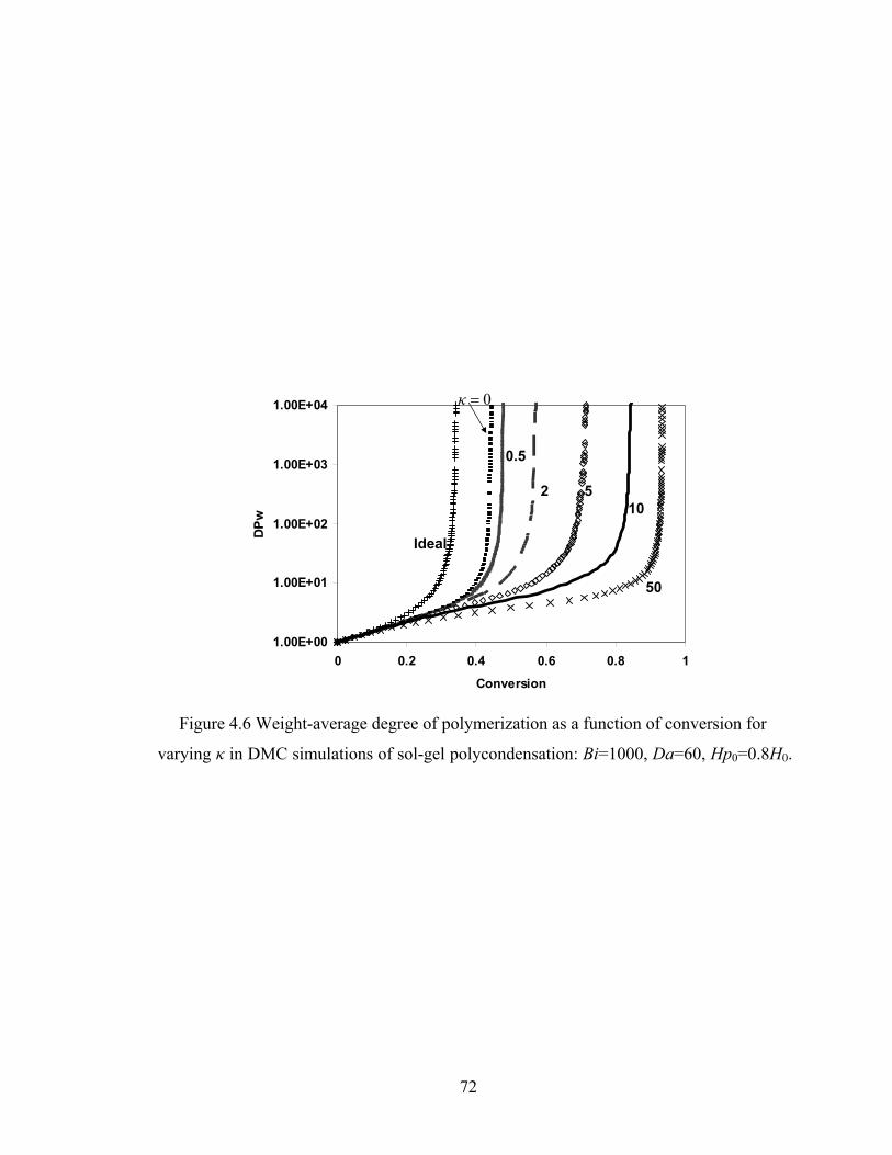
72

Figure 4.6 Weight-average degree of polymerization as a function of conversion for

varying κ in DMC simulations of sol-gel polycondensation: Bi=1000, Da=60, Hp0=0.8H0.

1.00E+00

1.00E+01

1.00E+02

1.00E+03

1.00E+04

0 0.2 0.4 0.6 0.8 1

Conversion

DPw

50

10 52

0.5

Ideal

0=κ

73

modeled by random branching theory (RBT), and the analytical gel conversion is

11−f

[71], where f is the number of polymerizable groups per monomer, which for silicon

sites is 4=f . In Figure 4.6, the gel conversion founded by DMC simulation of the ideal

case is about 0.33, consistent with the prediction of RBT. The case plotted for 0=κ is a

situation in which only the negative the first shell substitution effect (FSSE) described

above is allowed but which still excludes cyclization reactions. The estimated gel

conversion of the FSSE case is about 0.45, which agrees with the results obtained by

Kasehagen et al[39]. After adding unlimited cyclization in our multiscale model ( 0>κ ),

the gel conversion increases as the cyclization tendency κ increases, and for large κ the

gelation conversion can be even larger than 82%, which is the experimental value. It is

very clear from Figure 4.6 that cyclization delays the gelation. The results are consistent

with what Rankin et al[38] observed with their polycondensation model without drying.

The difference is that here drying is being simulated, and the results discussed are just for

one particular sol particle as it traverses through the film.

4.4.2 Wiener Index

Wiener index can be used as a measure of molecular compactness. Figure 4.7 shows

the scaled Wiener index (Wn / Wn,lin) as a function of conversion for varying κ in DMC

simulations. All the curves start from 1 and decrease with increasing conversion. That

means the molecules are becoming more compact than linear molecules of comparable

degree of polymerization would be. This is due to branching and cyclization (for 0≠κ ).

Since a negative FSSE results in polymers that are more linear than in the ideal

polycondensation case, the scaled index is larger for FSSE ( 0=κ ) and small values of κ

compared with ideal polycondensation. For a very large value of κ, e.g. 50=κ , three

regions are shown: first, the scaled index decreases and the value is even smaller than the

ideal case. This indicates that cyclization can shrink the molecular size so much that it

can offset or even override the effects of negative FSSE for molecular growth. After the

stage where W decreases (forming precursors), a plateau is reached. Growth of the

molecules becomes more important and the molecules maintain the same compactness

while growing. Finally, gelation is reached and the molecules become much more

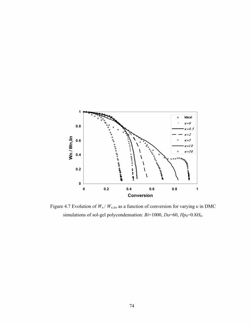
74

0

0.2

0.4

0.6

0.8

1

0 0.2 0.4 0.6 0.8 1

Conversion

Wn

/ Wn,

lin

Ideal

κ=0

κ=0.5

κ=2

κ=5

κ=10

κ=50

Figure 4.7 Evolution of Wn / Wn,lin as a function of conversion for varying κ in DMC

simulations of sol-gel polycondensation: Bi=1000, Da=60, Hp0=0.8H0.

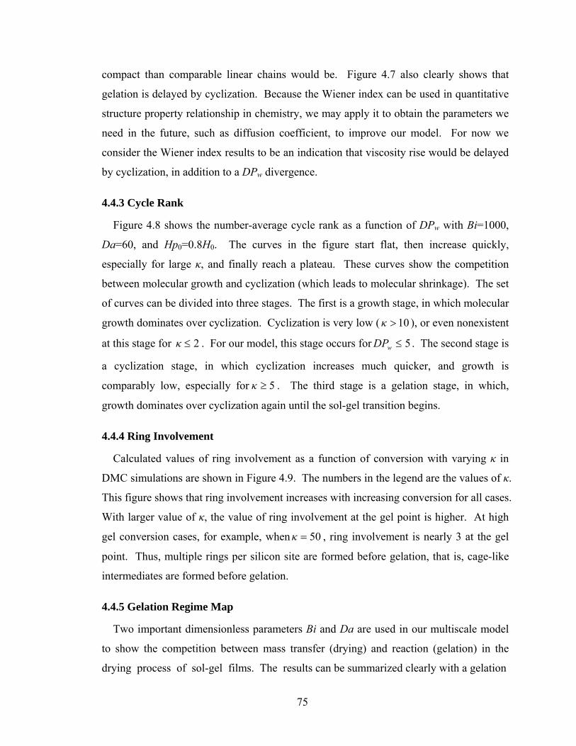
75

compact than comparable linear chains would be. Figure 4.7 also clearly shows that

gelation is delayed by cyclization. Because the Wiener index can be used in quantitative

structure property relationship in chemistry, we may apply it to obtain the parameters we

need in the future, such as diffusion coefficient, to improve our model. For now we

consider the Wiener index results to be an indication that viscosity rise would be delayed

by cyclization, in addition to a DPw divergence.

4.4.3 Cycle Rank

Figure 4.8 shows the number-average cycle rank as a function of DPw with Bi=1000,

Da=60, and Hp0=0.8H0. The curves in the figure start flat, then increase quickly,

especially for large κ, and finally reach a plateau. These curves show the competition

between molecular growth and cyclization (which leads to molecular shrinkage). The set

of curves can be divided into three stages. The first is a growth stage, in which molecular

growth dominates over cyclization. Cyclization is very low ( 10>κ ), or even nonexistent

at this stage for 2≤κ . For our model, this stage occurs for 5≤wDP . The second stage is

a cyclization stage, in which cyclization increases much quicker, and growth is

comparably low, especially for 5≥κ . The third stage is a gelation stage, in which,

growth dominates over cyclization again until the sol-gel transition begins.


Calculated values of ring involvement as a function of conversion with varying κ in

DMC simulations are shown in Figure 4.9. The numbers in the legend are the values of κ.

This figure shows that ring involvement increases with increasing conversion for all cases.

With larger value of κ, the value of ring involvement at the gel point is higher. At high

gel conversion cases, for example, when 50=κ , ring involvement is nearly 3 at the gel

point. Thus, multiple rings per silicon site are formed before gelation, that is, cage-like

intermediates are formed before gelation.


Two important dimensionless parameters Bi and Da are used in our multiscale model

to show the competition between mass transfer (drying) and reaction (gelation) in the

drying process of sol-gel films. The results can be summarized clearly with a gelation

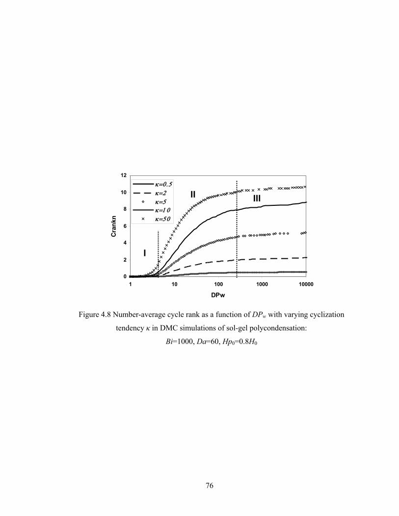
76

Figure 4.8 Number-average cycle rank as a function of DPw with varying cyclization

tendency κ in DMC simulations of sol-gel polycondensation:

Bi=1000, Da=60, Hp0=0.8H0

0

2

4

6

8

10

12

1 10 100 1000 10000

DPw

Cran

kn

κ=0.5κ=2κ=5κ=10κ=50

I

II III

77

0

0.5

1

1.5

2

2.5

3

0 0.2 0.4 0.6 0.8 1

Conversion

Rin

g In

volv

emen

t I

0.5251050gel point

Figure 4.9 Ring involvement as a function of conversion with varying cyclization

tendency κ in DMC simulations of sol-gel polycondensation:

Bi=1000, Da=60, Hp0=0.8H0. Circles represent gel points.

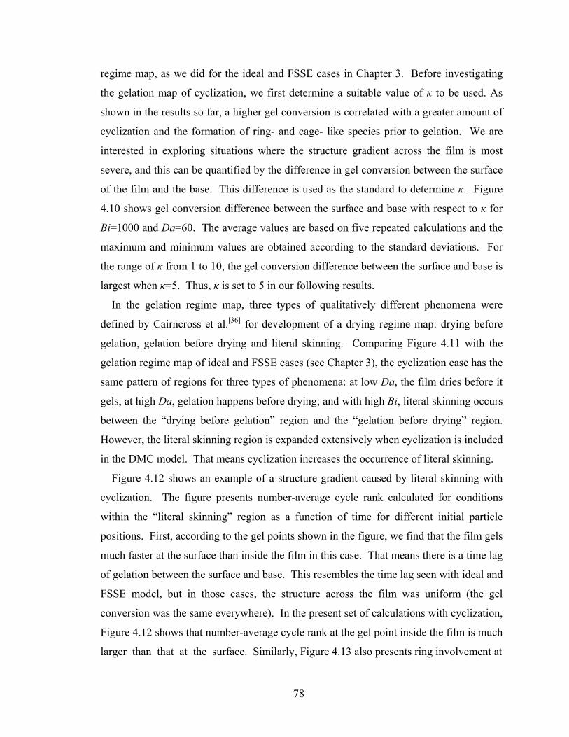
78

regime map, as we did for the ideal and FSSE cases in Chapter 3. Before investigating

the gelation map of cyclization, we first determine a suitable value of κ to be used. As

shown in the results so far, a higher gel conversion is correlated with a greater amount of

cyclization and the formation of ring- and cage- like species prior to gelation. We are

interested in exploring situations where the structure gradient across the film is most

severe, and this can be quantified by the difference in gel conversion between the surface

of the film and the base. This difference is used as the standard to determine κ. Figure

4.10 shows gel conversion difference between the surface and base with respect to κ for

Bi=1000 and Da=60. The average values are based on five repeated calculations and the

maximum and minimum values are obtained according to the standard deviations. For

the range of κ from 1 to 10, the gel conversion difference between the surface and base is

largest when κ=5. Thus, κ is set to 5 in our following results.

In the gelation regime map, three types of qualitatively different phenomena were

defined by Cairncross et al.[36] for development of a drying regime map: drying before

gelation, gelation before drying and literal skinning. Comparing Figure 4.11 with the

gelation regime map of ideal and FSSE cases (see Chapter 3), the cyclization case has the

same pattern of regions for three types of phenomena: at low Da, the film dries before it

gels; at high Da, gelation happens before drying; and with high Bi, literal skinning occurs

between the “drying before gelation” region and the “gelation before drying” region.

However, the literal skinning region is expanded extensively when cyclization is included

in the DMC model. That means cyclization increases the occurrence of literal skinning.

Figure 4.12 shows an example of a structure gradient caused by literal skinning with

cyclization. The figure presents number-average cycle rank calculated for conditions

within the “literal skinning” region as a function of time for different initial particle

positions. First, according to the gel points shown in the figure, we find that the film gels

much faster at the surface than inside the film in this case. That means there is a time lag

of gelation between the surface and base. This resembles the time lag seen with ideal and

FSSE model, but in those cases, the structure across the film was uniform (the gel

conversion was the same everywhere). In the present set of calculations with cyclization,

Figure 4.12 shows that number-average cycle rank at the gel point inside the film is much

larger than that at the surface. Similarly, Figure 4.13 also presents ring involvement at

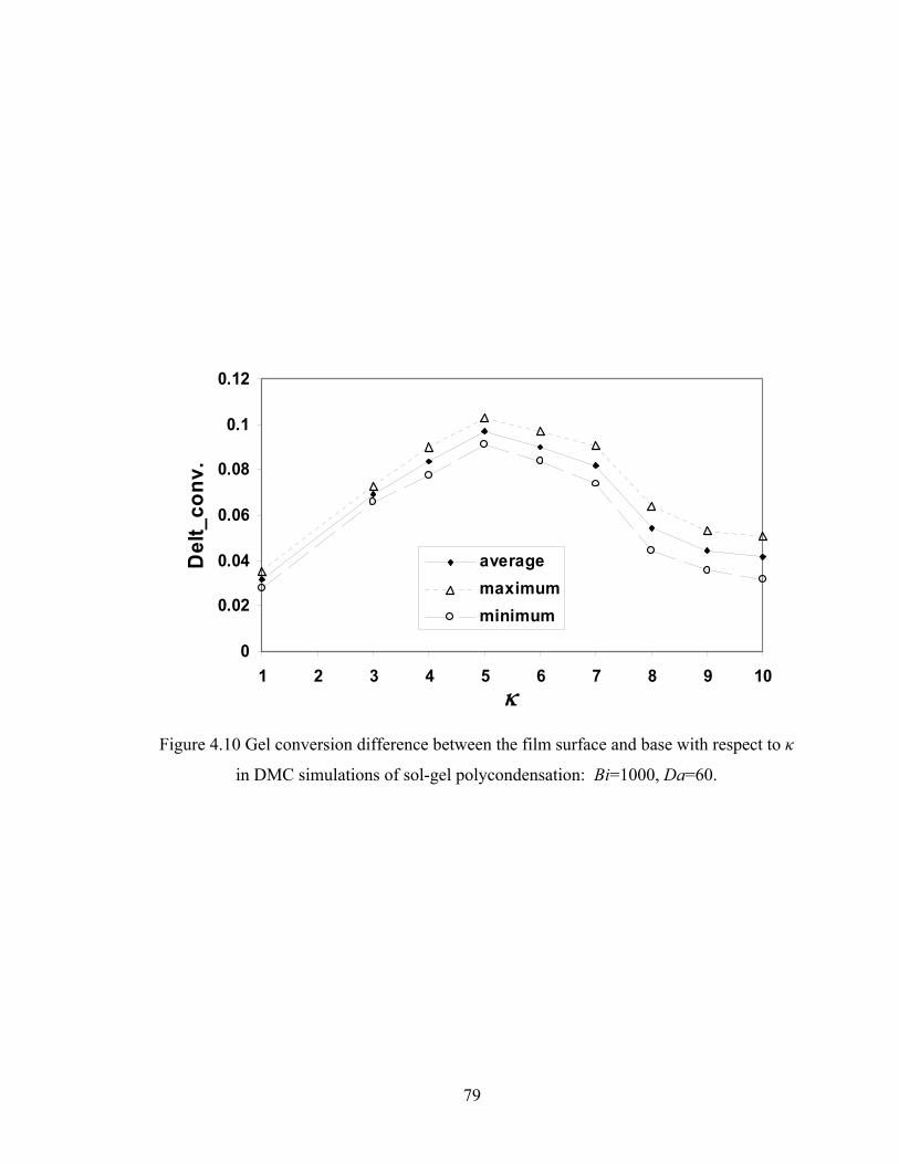
79

0

0.02

0.04

0.06

0.08

0.1

0.12

1 2 3 4 5 6 7 8 9 10κ

Del

t_co

nv.

averagemaximumminimum

Figure 4.10 Gel conversion difference between the film surface and base with respect to κ

in DMC simulations of sol-gel polycondensation: Bi=1000, Da=60.

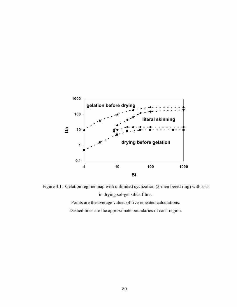
80

0.1

1

10

100

1000

1 10 100 1000

Bi

Da

Figure 4.11 Gelation regime map with unlimited cyclization (3-membered ring) with κ=5

in drying sol-gel silica films.





literal skinning

81

0

1

2

3

4

5

6

7

0 1 2 3 4Time

Cra

nkn hp0=0

hp0=0.4h0hp0=0.6h0hp0=0.8h0hp0=h0gel point

Figure 4.12 Number-average cycle rank as a function of time with different initial

particle positions for cyclization literal skinning case: Bi=1000, Da=60, κ=5.

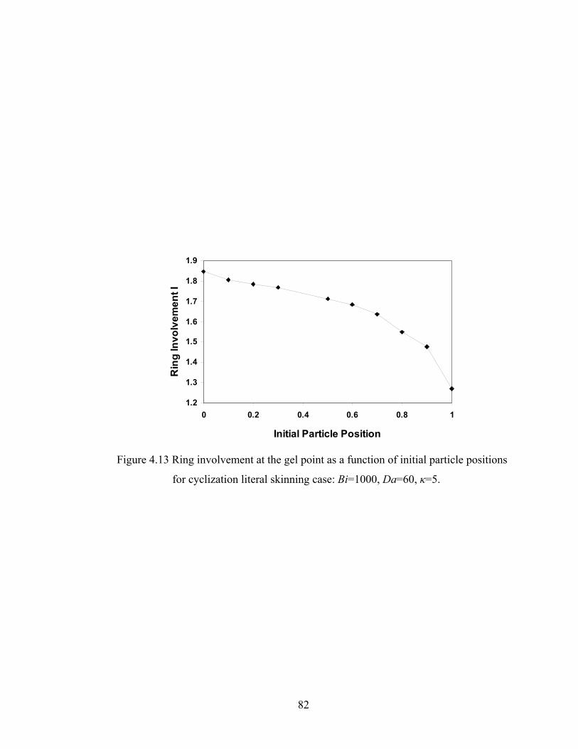
82

1.2

1.3

1.4

1.5

1.6

1.7

1.8

1.9

0 0.2 0.4 0.6 0.8 1

Initial Particle Position

Rin

g In

volv

emen

t I

Figure 4.13 Ring involvement at the gel point as a function of initial particle positions

for cyclization literal skinning case: Bi=1000, Da=60, κ=5.

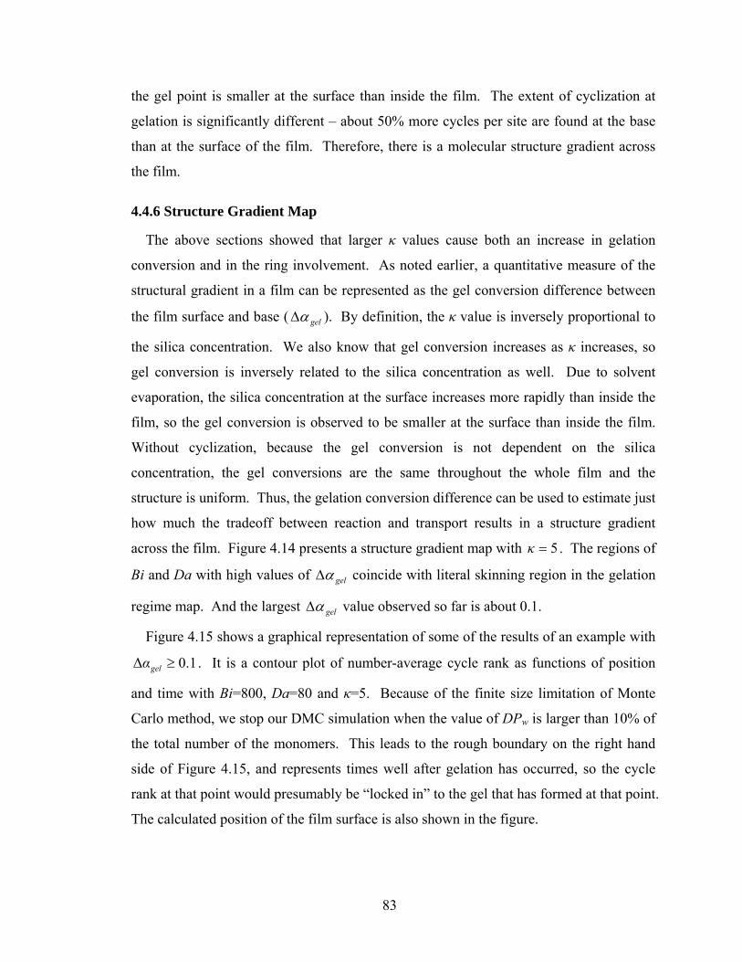
83

the gel point is smaller at the surface than inside the film. The extent of cyclization at

gelation is significantly different – about 50% more cycles per site are found at the base

than at the surface of the film. Therefore, there is a molecular structure gradient across

the film.

4.4.6 Structure Gradient Map

The above sections showed that larger κ values cause both an increase in gelation

conversion and in the ring involvement. As noted earlier, a quantitative measure of the

structural gradient in a film can be represented as the gel conversion difference between

the film surface and base ( gelαΔ ). By definition, the κ value is inversely proportional to

the silica concentration. We also know that gel conversion increases as κ increases, so

gel conversion is inversely related to the silica concentration as well. Due to solvent

evaporation, the silica concentration at the surface increases more rapidly than inside the

film, so the gel conversion is observed to be smaller at the surface than inside the film.

Without cyclization, because the gel conversion is not dependent on the silica

concentration, the gel conversions are the same throughout the whole film and the

structure is uniform. Thus, the gelation conversion difference can be used to estimate just

how much the tradeoff between reaction and transport results in a structure gradient

across the film. Figure 4.14 presents a structure gradient map with 5=κ . The regions of

Bi and Da with high values of gelαΔ coincide with literal skinning region in the gelation

regime map. And the largest gelαΔ value observed so far is about 0.1.

Figure 4.15 shows a graphical representation of some of the results of an example with

1.0Δ ≥gelα . It is a contour plot of number-average cycle rank as functions of position

and time with Bi=800, Da=80 and κ=5. Because of the finite size limitation of Monte

Carlo method, we stop our DMC simulation when the value of DPw is larger than 10% of

the total number of the monomers. This leads to the rough boundary on the right hand

side of Figure 4.15, and represents times well after gelation has occurred, so the cycle

rank at that point would presumably be “locked in” to the gel that has formed at that point.

The calculated position of the film surface is also shown in the figure.

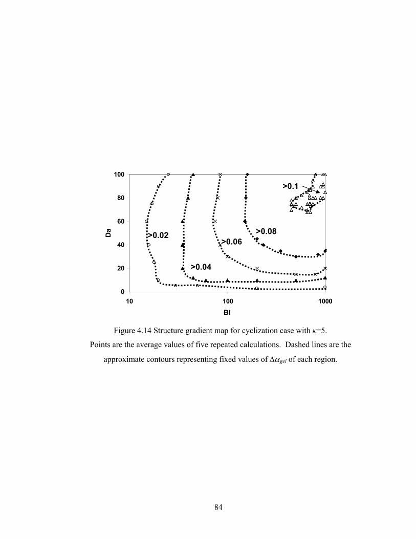
84

Figure 4.14 Structure gradient map for cyclization case with κ=5.

Points are the average values of five repeated calculations. Dashed lines are the

approximate contours representing fixed values of Δαgel of each region.

0

20

40

60

80

100

10 100 1000

Bi

Da

>0.06>0.08

>0.1

>0.02

>0.04

85

Figure 4.15 Example of contour plot of number-average cycle rank as functions of

position and time calculated with Bi=800, Da=80, and κ=5. The film surface is labeled,

and the contours end at times where DPw = 10% of the total number of monomers

(leading to the rough boundary on some contours).

Film Surface

86

4.4.7 The Effect of Solvent Vapor Pressure

We also examine the effects of solvent vapor pressure in our model by using two

different assumptions about solvent. One is the same as was used in previous

calculations – assuming that there is excess water in the solution and that all alcohol has

evaporated before the drying process starts, so water is the solvent. The second approach

is to assume that alcohol is the solvent and that whatever water was added to the sol was

completely consumed for hydrolysis (this may be true for methoxysilanes, for instance).

The results of assuming water as solvent have been shown above. In the following,

results of assuming alcohol as solvent are compared with those assuming water as solvent.

The differences between these two cases come from the different value of solvent vapor

pressure. Here, we use PE to denote the vapor pressure of ethanol and PW to denote the

vapor pressure of water.

Figure 4.16 shows the gelation regime map calculated using ethanol as solvent and

with κ=5. Compared with figure 4.11, all three regions are moved to higher values of Da

when Bi is smaller than 100. However, with high Bi (Bi>100), the conditions related to

each phenomenon are almost the same, while the literal skinning region is a little

expanded for smaller Bi. Figure 4.17 shows structural gradient map using ethanol as

solvent with κ=5. Compared with figure 4.14, the region of Bi and Da with largest value

of gelαΔ (>0.1) is almost the same (Bi>500), while other regions are shifted to smaller

values of Bi and Da.

Since solvent vapor pressure is a parameter related to the drying process, its value can

affect the results only when drying process is the rate-limiting process, that is, when Bi is

small. This explains why the differences of the results are shown only in the range with

small Bi. With the solvent vapor pressure increasing (the ethanol vapor pressure is larger

than water vapor pressure), the structural gradient is increased for the same values of Bi

and Da. Since our other results (Figure 4.6 to Figure 4.9) are based on large value of Bi

(Bi=1000), there are no major differences in these results due to the change in solvent

vapor pressure. Therefore, we don’t show the corresponding results of Figure 4.6 to

Figure 4.9 with ethanol vapor pressure.

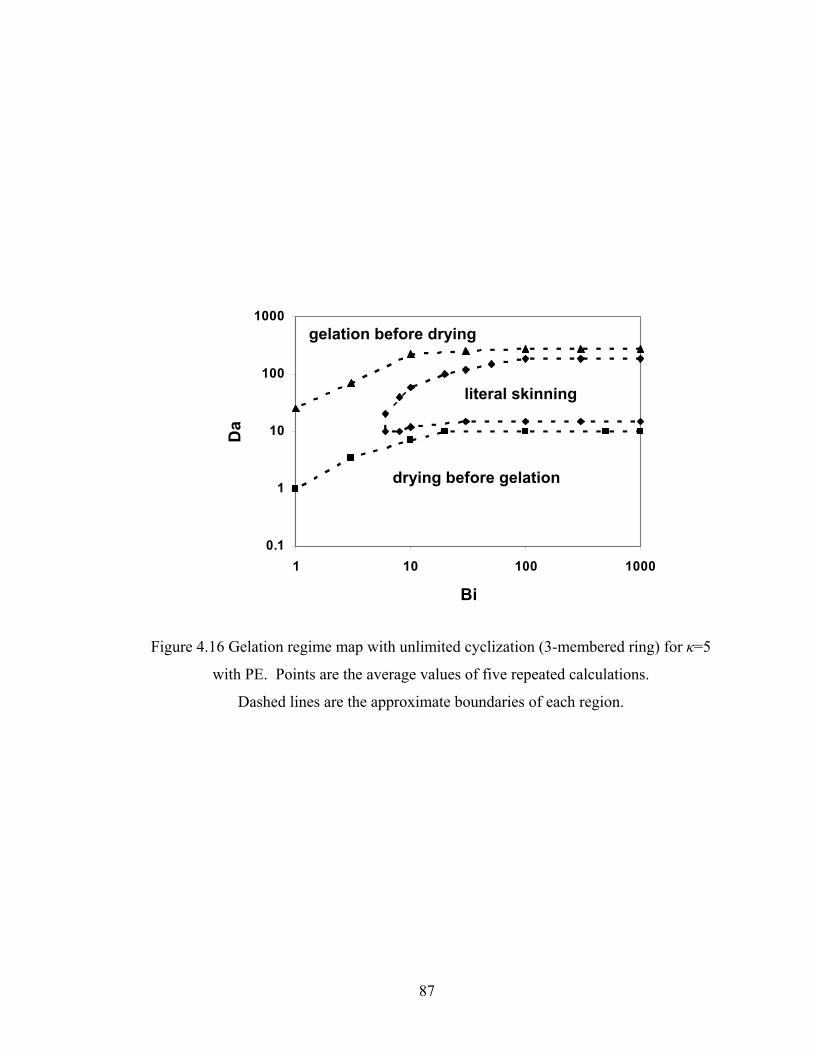
87

0.1

1

10

100

1000

1 10 100 1000

Bi

Da

Figure 4.16 Gelation regime map with unlimited cyclization (3-membered ring) for κ=5

with PE. Points are the average values of five repeated calculations.




literal skinning

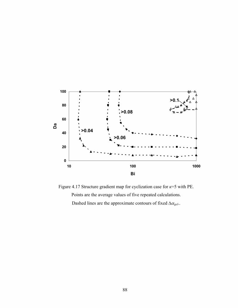
88

Figure 4.17 Structure gradient map for cyclization case for κ=5 with PE.


Dashed lines are the approximate contours of fixed Δαgel..

0

20

40

60

80

100

10 100 1000

Bi

Da

>0.1

>0.08

>0.06 >0.04

89

4.5 Summary

A multiscale model for the drying process of sol-gel films with unlimited cyclization

has been presented. Two main linkages between components of our multiscale model

were used: first, in the continuum model, the entire DMC simulation is treated as a

particle of sol whose position and composition are tracked using a diffusion / evaporation

finite difference calculation. Thus, the total silicon concentration, which is provided by

the continuum model, serves as one input parameter in the DMC model. Second, the

time interval used in the continuum model comes from the DMC simulation.

With assumptions of hydrolysis pseudoequilibrium and negative first shell substitution

effect for bimolecular and cyclization reactions, our model can predict that the gel

conversion increases with increasing cyclization tendency κ , and the gel conversion can

be equal to or larger than the experimental value (82%). In this paper, the Wiener index

has been introduced as a measure of molecular compactness. An efficient way is

described to update the Wiener index. The results clearly show that cyclization shrinks

the molecular size.

Competition between molecular growth and cyclization can be represented by curves

of number-average cycle rank as a function of weight-average degree of polymerization.

Three stages are obtained based on the results: i) A growth stage in which molecular

growth dominates over cyclization; ii) A cyclization stage where cyclization increases

much quicker than the first stage, and growth is slow, especially for 5≥κ ; and iii) A

gelation stage where growth dominates over cyclization again until the sol-gel transition

begins.

The gelation regime map shows the effects of the competition between mass transfer

(drying) and reaction (gelation) on the drying process of the sol-gel film. Compared with

similar maps for the ideal and FSSE cases, the DMC model with unlimited 3-membered

rings has the same tendency to generate three types of phenomena: drying before gelation,

literal skinning and gelation before drying. The difference is that the literal skinning

region is expanded with cyclization. In other words, cyclization increases the likelihood

of literal skinning.

The relationship between ring involvement and conversion with different κ and initial

particle positions was investigated. The simulations showed that cage-like intermediates

90

form before gelation at high gel conversion cases (with large κ ). With drying the

maximum value of ring involvement inside the film is much larger in some cases than

that at the surface, suggesting that cyclization can lead to a molecular structure gradient

inside the film.

Although by now our model just considers forming 3-membered rings, it is the first

model to couple unlimited cyclization in a DMC model of polycondensation with

continuum mass transfer processes. It is the first model that can predict structure

gradients across drying sol-gel films due to cyclization. The simulations that predict high

values of gel conversion gradient between surface and base coincide with the literal

skinning region in the gelation regime map.

This multiscale model is our first step to understand the drying process of sol-gel

coating with unlimited 3-membered rings cyclization. However, experiments have

shown that 4-membered rings are the dominant structural unit[47, 49, 56]. Therefore a model

with unlimited 4-membered rings should give better quantitative predictions. We present

the results of this modeling in Chapter 5. And, because Wiener index can be used in

quantitative structure property relationship in chemistry, we can apply it to obtain the

parameters we need in the future, such as diffusion coefficient, to further improve our

model.

91

Chapter 5

Multiscale Modeling with Unlimited 4-membered Ring Cyclization

5.1 Introduction

Sol-gel silica films and related polycondensation networks are of growing interest in

industrial practice and as sources of novel materials[1]. In particular, there has been an

explosive growth in the design of mesoporous and macroporous silica-based thin films in

the last decade, which is based on the slow formation of a silica gel near ambient

conditions in the presence of a structure-directing agent[1, 99, 100]. The coating process of

forming sol-gel silica films couples polymerization and drying, i.e., it involves multiple

length and time scales ranging from molecular to macroscopic. Therefore, a multiscale

model is necessary to link different length and time scales together throughout the entire

simulated domain.

At the molecular scale of the sol-gel silica polymerization process, cyclization occurs

as a nonrandom, preferential reaction[40-42] and delays gelation to a siloxane bond

conversion of about 82%[43-45] (this value can be compared to a value of 33% expected

for random, ideal polycondensation). Large concentrations of 3- and 4-membered rings

containing species have also been found during sol-gel silica polymerization by different

analytical techniques[27, 40-42, 44, 46-56]. Therefore, cyclization should be taken into account

in the polymerization process modeling. Rankin et al.[38] were the first group to present a

polymerization model with extensive cyclization to model the formation of polycyclic

structures containing 3-membered rings. They used the concept of bond blocks

(contiguous paths of discrete numbers of bonds that occur in the population of oligomers)

to calculate cyclization reaction rates and applied the dynamic Monte Carlo (DMC)

technique to the simulation of the polymerization process. In our previous chapter, we

added unlimited 3-membered ring cyclization into our multiscale DMC / continuum

model as our first step to investigate the effects of cyclization on the sol-gel silica film

coating process. However, experiments show that 4-membered rings dominate over and

are more stable structural units than 3-membered rings in real silicates[47-49, 53, 56]. A

92

polymerization model allowing the formation of 4-membered rings should give better

qualitative and quantitative predictions than those allowing only intermolecular reactions

(even with substitution effects) or only 3-membered rings. Based on our previous work

with a model allowing unlimited formation of 3-membered rings, we will describe a new

multiscale model with unlimited 4-membered ring formation. While it seems to be a

simple extension of the 3-membered ring polymerization model, accounting for all

possible types of 3-bond blocks and their evolution during polymerization introduced

challenges that needed to be addressed. Most importantly, the new approach brings the

prediction of cyclization into a physically reasonable concentration range for the first

time.

In this chapter, we first briefly review DMC simulation of sol-gel silica kinetics[27, 31, 36,

38, 39] with a particular focus on our new algorithm for 4-membered rings cyclization.

Then, the continuum model to which the DMC method is coupled is formulated based on

macroscopic conservation equations for mass, and expressed by a set of partial

differential equations for species concentrations with initial and boundary conditions.

The entire DMC simulation is treated as a particle of sol whose position and composition

are tracked in the continuum model. Linking the two models is accomplished by

synchronizing time steps and concentrations between the continuum and DMC models

while tracking the positions of sol particles during drying. After introducing the model,

we present the results of simulations of small swarms of sol particles starting from

different positions in the film. The effect of dimensionless cyclization tendency on the

gel point, cycle rank and ring involvement are calculated and discussed. The multiscale

modeling approach allows us to observe the competition between growth and cyclization,

and between drying and gelation. We will compare the quantitative predictions of the

new 4-membered ring calculations with those based only on 3-membered rings.

5.2 DMC Model

5.2.1 Bimolecular Condensation

With the simplification that hydrolysis is assumed to be at pseudoequilibrium, that

only a first shell substitution effect for condensation needs to be considered and that

93

alcohol-producing condensation can be neglected, the bimolecular rate expressions are

given (as in Chapters 3-4) by [38]:

⎪⎩

⎪⎨⎧

=−−

≠−−=

jiQQjfifk

jiQQjfifkR

jiij


21

],][)[)((*

*

(5.1)

5.2.2 Four-membered Ring Cyclization

A cyclization reaction occurs when the two sites chosen to react are in the same

molecule. This intramolecular reaction causes a new ring to form. Usually in DMC

simulations, if the sites chosen to react by a bimolecular reaction are members of the

same molecule, they are not allowed to react. This prevents unrealistic random

intramolecular reactions from occurring at a rate that does not take into account the

bonding restrictions that favor certain sizes of rings. Similar to the previous chapter

regarding 3-membered rings, we use bond blocks ijn B to explicitly calculate cyclization

rates based on quasi-unimolecular reactions of these structural units. Here the superscript

n represents the number of siloxane (Si-O-Si) bonds linking one site to another, and the

subscripts i and j represent the connectivities of the sites at the ends of the block (i.e. the

numbers of siloxane bonds attached to each end). Since 4-membered rings are prevalent

and more stable than 3-membered rings in real silicates, we model cyclization reactions

to form only 4-membered rings. Therefore, we just need to pay attention to three-bond

blocks. Based on this approach, the rates of cyclization reactions are calculated as[38]:

][))(( 3*),(4

4ijjic

cycij BkjfifR −−= , =ji & 1, 2, 3. (5.2)

where *),(4 jick is the rate coefficient for a bond block terminated with Qi and Qj sites and

[3Bij] is the concentration of 3-bond blocks. Assuming that the same substitution effect

applies to ring closure even in the presence of the geometric restriction from the bond

block, the following rate coefficients are used:

⎥⎥⎥

⎦

⎤

⎢⎢⎢

⎣

⎡=

01.009.01.081.09.00.1

*)1,1(4

*4 cc kK .

We use the same dimensionless parameter κ as defined by Rankin et al.[38] to represent

the cyclization tendency of the system

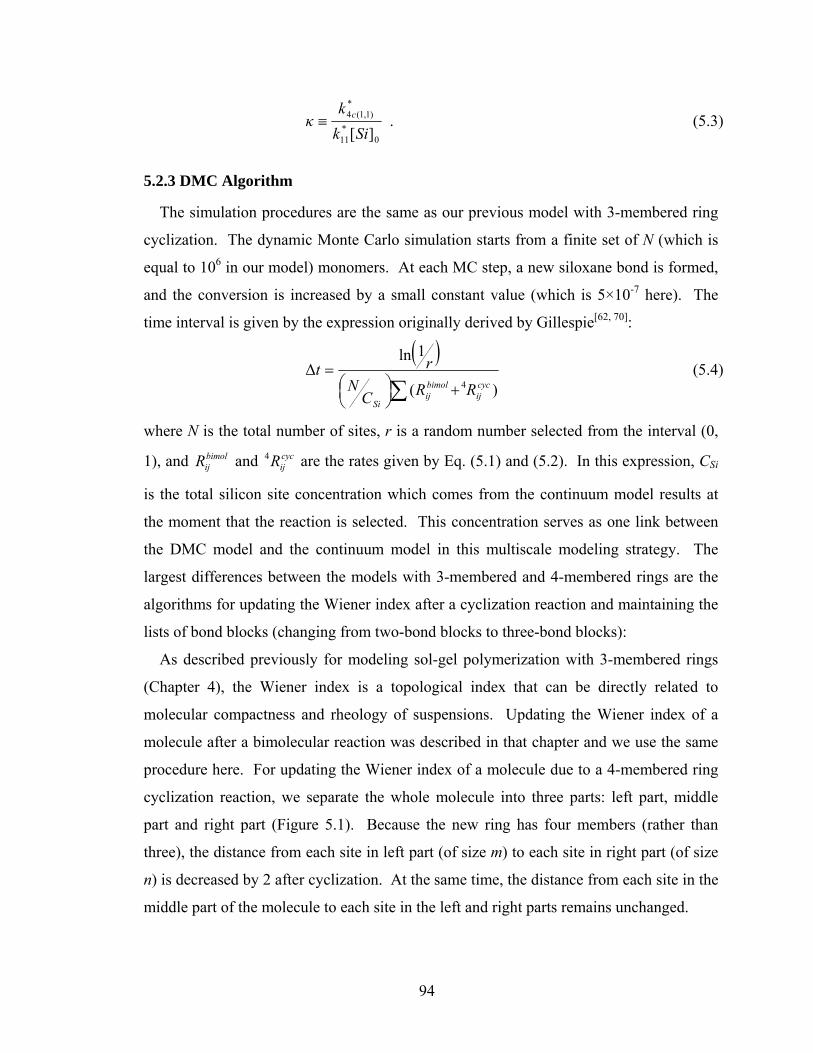
94

0

*11

*)1,1(4

][Sikk

κ c≡ . (5.3)

5.2.3 DMC Algorithm

The simulation procedures are the same as our previous model with 3-membered ring

cyclization. The dynamic Monte Carlo simulation starts from a finite set of N (which is

equal to 106 in our model) monomers. At each MC step, a new siloxane bond is formed,

and the conversion is increased by a small constant value (which is 5×10-7 here). The

time interval is given by the expression originally derived by Gillespie[62, 70]:

( )

∑ +⎟⎠⎞⎜

⎝⎛

=)(

1lnΔ

4 cycij

bimolij

SiRRC

Nrt (5.4)

where N is the total number of sites, r is a random number selected from the interval (0,

1), and bimolijR and cyc

ijR4 are the rates given by Eq. (5.1) and (5.2). In this expression, CSi

is the total silicon site concentration which comes from the continuum model results at

the moment that the reaction is selected. This concentration serves as one link between

the DMC model and the continuum model in this multiscale modeling strategy. The

largest differences between the models with 3-membered and 4-membered rings are the

algorithms for updating the Wiener index after a cyclization reaction and maintaining the

lists of bond blocks (changing from two-bond blocks to three-bond blocks):

As described previously for modeling sol-gel polymerization with 3-membered rings

(Chapter 4), the Wiener index is a topological index that can be directly related to

molecular compactness and rheology of suspensions. Updating the Wiener index of a

molecule after a bimolecular reaction was described in that chapter and we use the same

procedure here. For updating the Wiener index of a molecule due to a 4-membered ring

cyclization reaction, we separate the whole molecule into three parts: left part, middle

part and right part (Figure 5.1). Because the new ring has four members (rather than

three), the distance from each site in left part (of size m) to each site in right part (of size

n) is decreased by 2 after cyclization. At the same time, the distance from each site in the

middle part of the molecule to each site in the left and right parts remains unchanged.

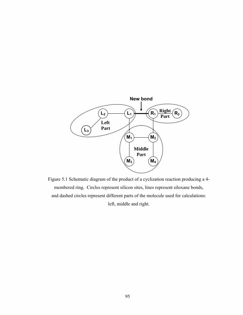
95

Figure 5.1 Schematic diagram of the product of a cyclization reaction producing a 4-

membered ring. Circles represent silicon sites, lines represent siloxane bonds,

and dashed circles represent different parts of the molecule used for calculations:

left, middle and right.

Middle Part

L2

L3

L1

New bond

R1 R2

M1 M2

M3 M4

Left Part

Right Part

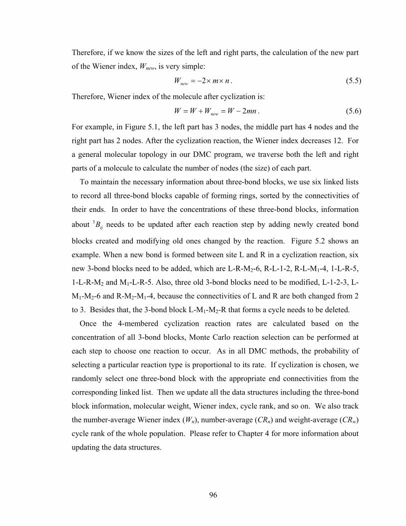
96

Therefore, if we know the sizes of the left and right parts, the calculation of the new part

of the Wiener index, Wnew, is very simple:

nmWnew ××−= 2 . (5.5)

Therefore, Wiener index of the molecule after cyclization is:

mnWWWW new 2−=+= . (5.6)

For example, in Figure 5.1, the left part has 3 nodes, the middle part has 4 nodes and the

right part has 2 nodes. After the cyclization reaction, the Wiener index decreases 12. For

a general molecular topology in our DMC program, we traverse both the left and right

parts of a molecule to calculate the number of nodes (the size) of each part.

To maintain the necessary information about three-bond blocks, we use six linked lists

to record all three-bond blocks capable of forming rings, sorted by the connectivities of

their ends. In order to have the concentrations of these three-bond blocks, information

about ijB3 needs to be updated after each reaction step by adding newly created bond

blocks created and modifying old ones changed by the reaction. Figure 5.2 shows an

example. When a new bond is formed between site L and R in a cyclization reaction, six

new 3-bond blocks need to be added, which are L-R-M2-6, R-L-1-2, R-L-M1-4, 1-L-R-5,

1-L-R-M2 and M1-L-R-5. Also, three old 3-bond blocks need to be modified, L-1-2-3, L-

M1-M2-6 and R-M2-M1-4, because the connectivities of L and R are both changed from 2

to 3. Besides that, the 3-bond block L-M1-M2-R that forms a cycle needs to be deleted.

Once the 4-membered cyclization reaction rates are calculated based on the

concentration of all 3-bond blocks, Monte Carlo reaction selection can be performed at

each step to choose one reaction to occur. As in all DMC methods, the probability of

selecting a particular reaction type is proportional to its rate. If cyclization is chosen, we

randomly select one three-bond block with the appropriate end connectivities from the

corresponding linked list. Then we update all the data structures including the three-bond

block information, molecular weight, Wiener index, cycle rank, and so on. We also track

the number-average Wiener index (Wn), number-average (CRn) and weight-average (CRw)

cycle rank of the whole population. Please refer to Chapter 4 for more information about

updating the data structures.

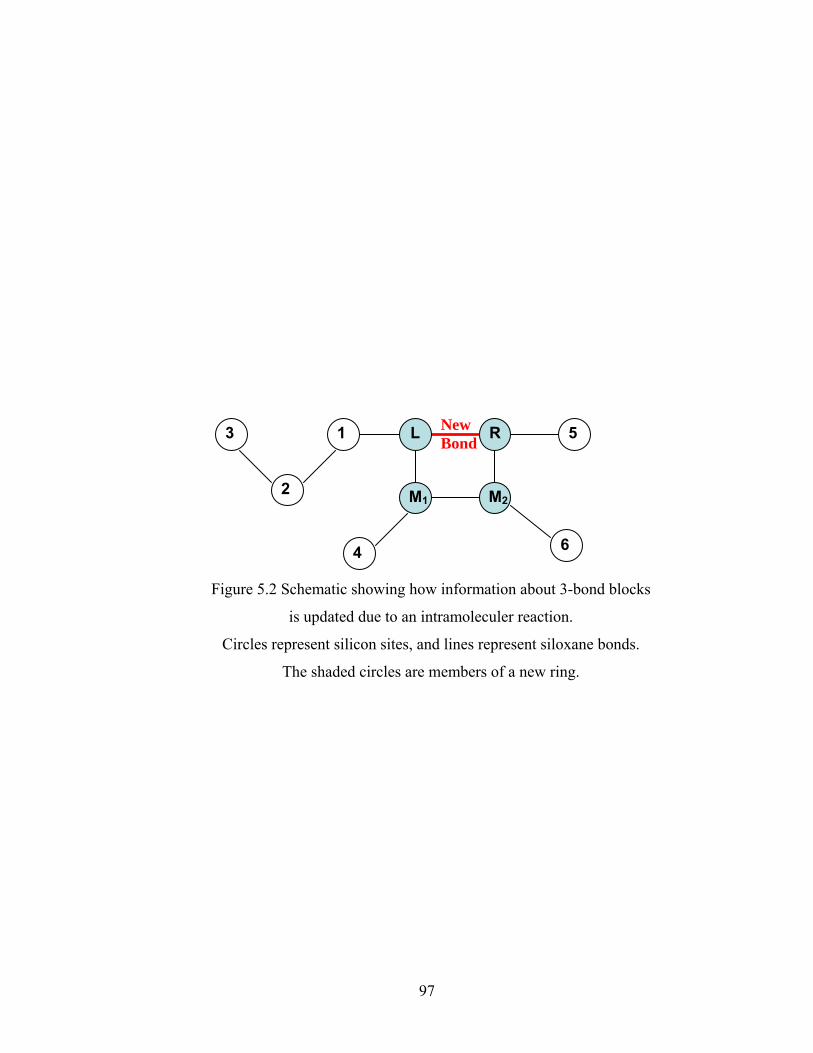
97

Figure 5.2 Schematic showing how information about 3-bond blocks

is updated due to an intramoleculer reaction.

Circles represent silicon sites, and lines represent siloxane bonds.

The shaded circles are members of a new ring.

6

M2

5 R

2

1

4

L

M1

3 New Bond

98

Using the DMC approach, we are able to explicitly track all information about three-

bond blocks formed and consumed in the course of polymerization, and then to use this

information to calculate the cyclization rates. This is the advantage of the DMC method

compared with statistical models, which assume that bond block populations can be

derived from the populations of constituent sites. Even the hybrid Monte Carlo /

spanning-tree model of Sarmoria and Miller used the Monte Carlo method just to sample

the populations of bond blocks about a given site based on randomly joining sites

according to the polymerization conversion[101]. This approach is likely to introduce

systematic errors for highly non-random polymerization such as the polymerization we

are modeling here. Another advantage of the DMC approach is that we can obtain

structural parameters including the gel point, molecular weight distribution, Wiener index,

etc., which are related to film microstructure and are not available from a continuum

kinetic model.


5.3.1 Model description

The 1D continuum transport model for the formation of sol-gel thin-film coatings is

exactly the same as the one described in our previous multiscale modeling work (Chapter

4). It is developed from macroscopic conservation equations for mass. It is a simplified

one-dimensional model corresponding to a rapidly deposited film that begins drying and

curing after the coating process is complete. Via evaporation, solvent departs the film

continuously at the top liquid / vapor interface. In addition to this evaporation, the

diffusion of solvent within the film needs to be included in the model. Please refer to

Chapter 4 for the assumptions and discussion of the modeling equations. Here, we

assume that alcohol (ethanol) is the sole solvent.

5.3.2 Governing equations

Assuming only diffusion inside of the film, the governing equations are simply written

as follows: 2

1 11 2 0C CD

t z∂ ∂

− =∂ ∂

(5.7)

99

22 2

2 2 0C CDt z

∂ ∂− =

∂ ∂ (5.8)

where C1 is the concentration of solvent, C2 is the total silicon concentration, and D is the

diffusion coefficient for each species.

Initial conditions in this formulation are as follows:

( ) 0,11 ,0 CzC = ; ( ) 0,22 ,0 CzC = ; (5.9)

Consistent with the description of the film model described above, the boundary

conditions are given by:

At the substrate ( 0=z ): 0=∂∂

zCD i

i ( =i 1, 2); (5.10)

At the free surface ( )(tHz = ): 11 1 1 1

( ) ( )sg

C dH tD C k y yz dt

∞∂− − = −

∂ (5.11)

z

CVV

zC

∂∂

−=∂∂ 1

2

12

ˆˆ

(5.12)

In Eq. (5.11), gk is the mass transfer coefficient of solvent in the vapor phase, 1sy is the

molar fraction of solvent just above the film surface in the gas phase (which is calculated

based on Raoult’s law), and 1y∞ is the molar fraction of solvent in the gas phase far away

from the film, which is set to zero here. The rate of change of film thickness, as known

as the surface velocity vs, can be calculated according to the following expression:

1 1 1( ) ˆ ( )s s

gdH t v V k y y

dt∞= = − − , (5.13)

In Eq. (5.12), 0,2

10,12

ˆ1ˆC

VCV

−= , where iV is the molar volume of species i.


The following dimensionless variables are defined to solve the transport equations

numerically:

)(/ tHzη = , 0/)( HtHh = , 0/ CCc ii = , tHDτ 2

1= . (5.14)

Using the dimensionless variableη , the region in which diffusion occurs is always from

0=η to 1=η . In other words, the physical moving domain is mapped onto a fixed

100

domain, and we do not need to modify the spatial grid during the simulation. The

parameters are the same as those in Chapter 4.

This set of dimensionless equations is numerically solved using explicit centered finite

difference method. We discretize the whole domain into a number of thin slices; each

one has a fixed thickness ηΔ . For the solution, the time interval ∆t is equal to the time

interval between reactions estimated from the DMC simulation. At each finite difference

step, we use the concentrations, film thickness, the surface velocity, and Robin boundary

conditions at the surface from the previous time step to complete the calculation. The

entire DMC simulation is treated as a particle of sol whose position and composition are

tracked in the continuum model. We use linear interpolation to perform the tracking (see

Chapter 3) and obtain total silicon site concentration, which is supplied to the DMC

routine to choose the next reaction and calculate the time interval of the next DMC step,

as discussed earlier.

5.4 Results and discussion

As in our previous chapter about forming 3-membered rings, we will present the

results of the multiscale model with 4-membered rings in terms of conversion, number-

average Wiener index, cycle rank, ring involvement, gelation regime map and structure

gradient map. Some of these results will be compared with the results of a model

allowing only 3-membered rings.

5.4.1 Conversion at Gelation

Figure 5.3 shows the weight-average degree of polymerization (DPw) calculated by the

model with 4-membered rings as a function of conversion for a specific set of drying

conditions, for varying values of κ. The divergence of the curve indicates the onset of

gelation. Similar with the results of the model with unlimited 3-membered rings, the gel

conversion increases as cyclization tendency κ increases. It is very obvious that

cyclization delays gelation, and that for some values of κ, the gel conversion can be as

large as or larger than the experimental value for tetraalkoxysilanes (82%).

The gel conversions as a function of dimensionless cyclization tendency κ for models

with 3- or 4-membered rings are compared in Figure 5.4. There are no major differences

of gel conversions between simulations with the two types of rings. The curves can still

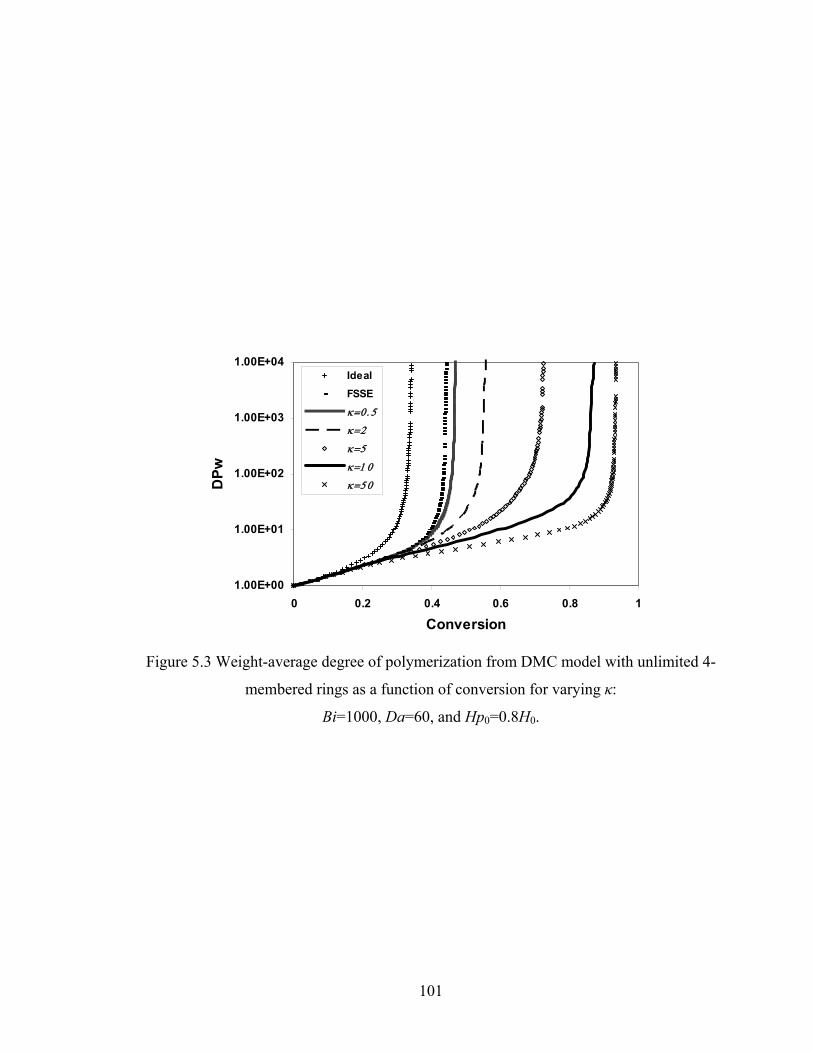
101

1.00E+00

1.00E+01

1.00E+02

1.00E+03

1.00E+04

0 0.2 0.4 0.6 0.8 1

Conversion

DPw

IdealFSSEκ=0 .5

κ=2

κ=5

κ=10

κ=50

Figure 5.3 Weight-average degree of polymerization from DMC model with unlimited 4-

membered rings as a function of conversion for varying κ:

Bi=1000, Da=60, and Hp0=0.8H0.

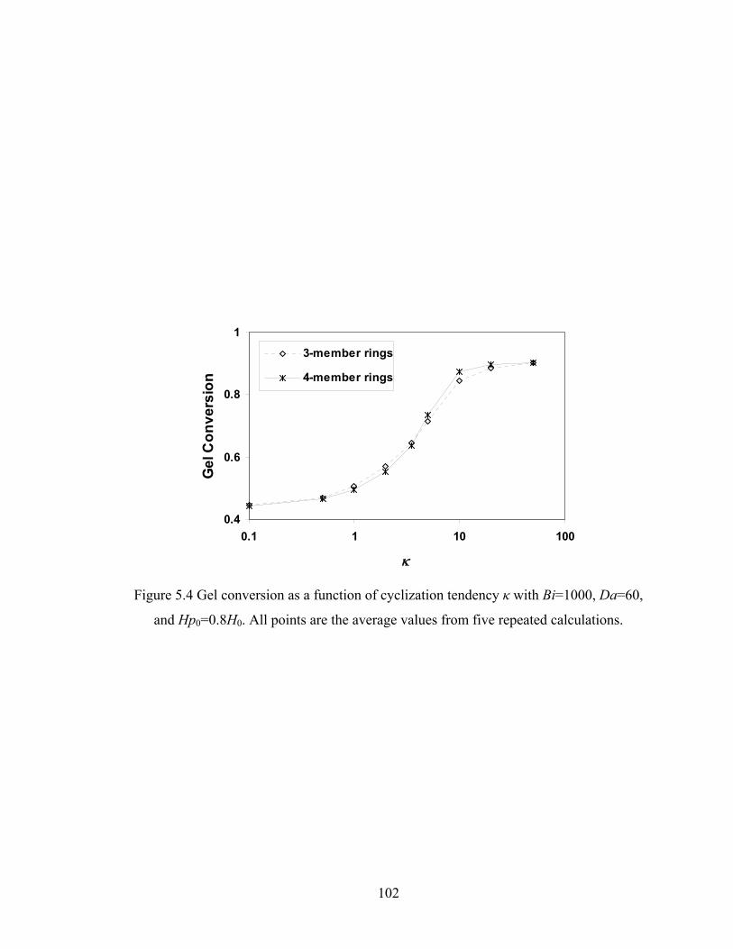
102

0.4

0.6

0.8

1

0.1 1 10 100

κ

Gel

Con

vers

ion

3-member rings

4-member rings

Figure 5.4 Gel conversion as a function of cyclization tendency κ with Bi=1000, Da=60,

and Hp0=0.8H0. All points are the average values from five repeated calculations.

103

be divided into several parts: when 5.0≤κ or 50≥κ , gel conversions are almost

constant with respect to κ for both cases. When 5.31 ≤≤ κ , gel conversions with 3-

membered rings are a little larger than with 4-membered rings. When 205 ≤≤ κ , on the

other hand, gel conversions of 4-membered rings cyclization are a little larger than those

of 3-membered rings cyclization. This transition from the range of κ giving almost no

cyclization ( 5.0≤κ ) to the range of κ giving cage-like precursor formation before

gelation ( 50≥κ ) is sharper in the model with 4-membered rings. However, the

assumptions behind the model with 4-membered rings are more realistic. Experiments

have shown that 3-membered ring formation is reversible, at least in the case of methyl-

modified precursors[27], which has not been accounted for in our model (but which would

presumably cause lower conversions at gelation with 3-membered rings). Also, the

experimental value of κ is about twice as large for 4-membered rings (see below), which

would favor the high conversions at gelation observed experimentally.

As we mentioned before, at each MC step, a new siloxane bond is formed, and the

conversion is increased by a small constant value (which is 5×10-7 in our model). So in

fact, the gel conversion is determined by the total number of MC steps required to reach

the gel point. We can divide the total MC steps into two parts:

cbt SSS += , (5.15)

where St is the total number of MC steps at the gel point, Sb is the number of bimolecular

reactions steps and Sc is the number of cyclization reactions.

At each bimolecular reaction step, the total number of molecules decreases by one,

while at each cyclization reaction step, the total number of molecules remains the same.

We keep track of the numbers of reaction steps for 50=κ and show the results in Table

5.1. This table shows that more bimolecular reactions occur in the 4-membered ring case

than with 3-membered rings. This suggests that at gelation, the total number of

molecules in the 4-membered ring system is smaller than in the 3-membered ring system.

The net result (as we will discuss below) is a higher number-average cycle rank with 4-

membered rings, although the absolute number of rings per site in the simulation is less.

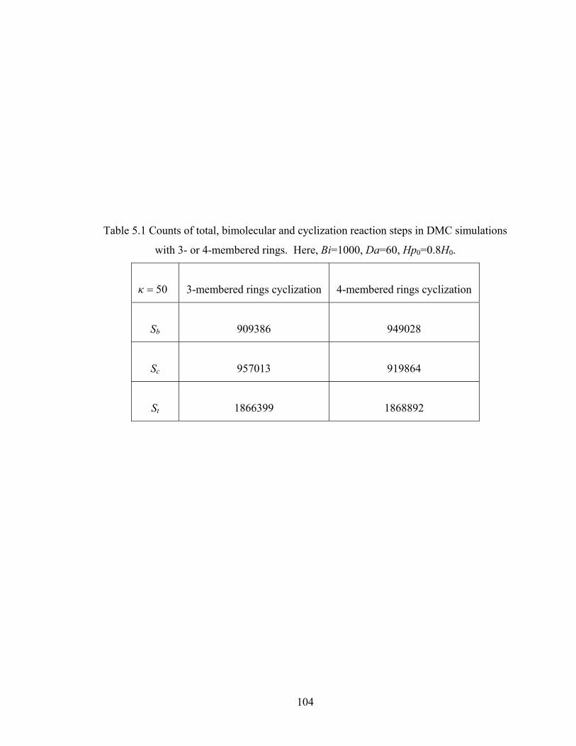
104

Table 5.1 Counts of total, bimolecular and cyclization reaction steps in DMC simulations

with 3- or 4-membered rings. Here, Bi=1000, Da=60, Hp0=0.8H0.

50=κ

3-membered rings cyclization

4-membered rings cyclization

Sb

909386

949028

Sc

957013

919864

St

1866399

1868892

105

5.4.2 Wiener Index

Molecular compactness can be measured by the Wiener index. Figure 5.5 shows the

scaled Wiener index (Wn / Wn,lin) as a function of conversion for varying κ in DMC

simulations. All the curves start from 1 and decrease with increasing conversion. That

means the molecules are becoming more compact than linear molecules of comparable

degree of polymerization would be. This is due to branching and cyclization (for 0≠κ ).

Since a negative FSSE results in polymers that are more linear than in the ideal

polycondensation case, the scaled index is larger at a given conversion for FSSE ( 0=κ )

and cyclization (for 0≠κ ) compared with ideal polycondensation. Figure 5.5 also

clearly shows that cyclization delays the gelation.

Compared with results of 3-membered ring case (Figure 5.5’), the only difference

exists in the region where 2.0<α with 50=κ . In this region, the value of scaled index

with 50=κ is identical to or larger than that of ideal case for 4-membered ring

cyclization, while the opposite is observed for the 3-membered ring case – the value of

scaled index with 50=κ is smaller than that of ideal case. This is because 3-bond

blocks are formed later than 2-bond blocks, so 4-membered ring cyclization reactions

start later and occur less in the beginning of the polycondensation process than for 3-

membered rings. For 15.0<α , it is also possible that the compaction effect of 4-

membered ring cyclization can offset the effects of negative FSSE for molecular growth.

Therefore, the curve of 50=κ behaves like the ideal case for 15.0<α .

5.4.3 Cycle Rank

The cycle rank of an oligomer represents the number of independent cycles that must

be closed in order to form that structure[38]. Figure 5.6 shows the number-average cycle

rank for simulations with 4-membered rings and various κ values as a function of DPw.

Compared with Figure 5.6’, the curves have same tendencies as for simulations with 3-

membered rings and also show the competition between molecular growth and

cyclization. Models with both types of cyclization can be divided into three stages:

growth stage (I), cyclization stage (II) and gelation stage (III). When κ is smaller than 2,

the values of number-average cycle rank of models with both ring sizes are almost

identical. However, with increasing κ (especially when 5≥κ ), the number-average cycle

106

0.0

0.2

0.4

0.6

0.8

1.0

0 0.2 0.4 0.6 0.8 1Conversion

Wn/

Wn,

lin

Idealκ=0κ=0.5κ=2κ=5κ=10κ=50

Figure 5.5 Evolution of Wn / Wn,lin as a function of conversion for varying κ in DMC

simulations with 4-membered rings: Bi=1000, Da=60, Hp0=0.8H0.

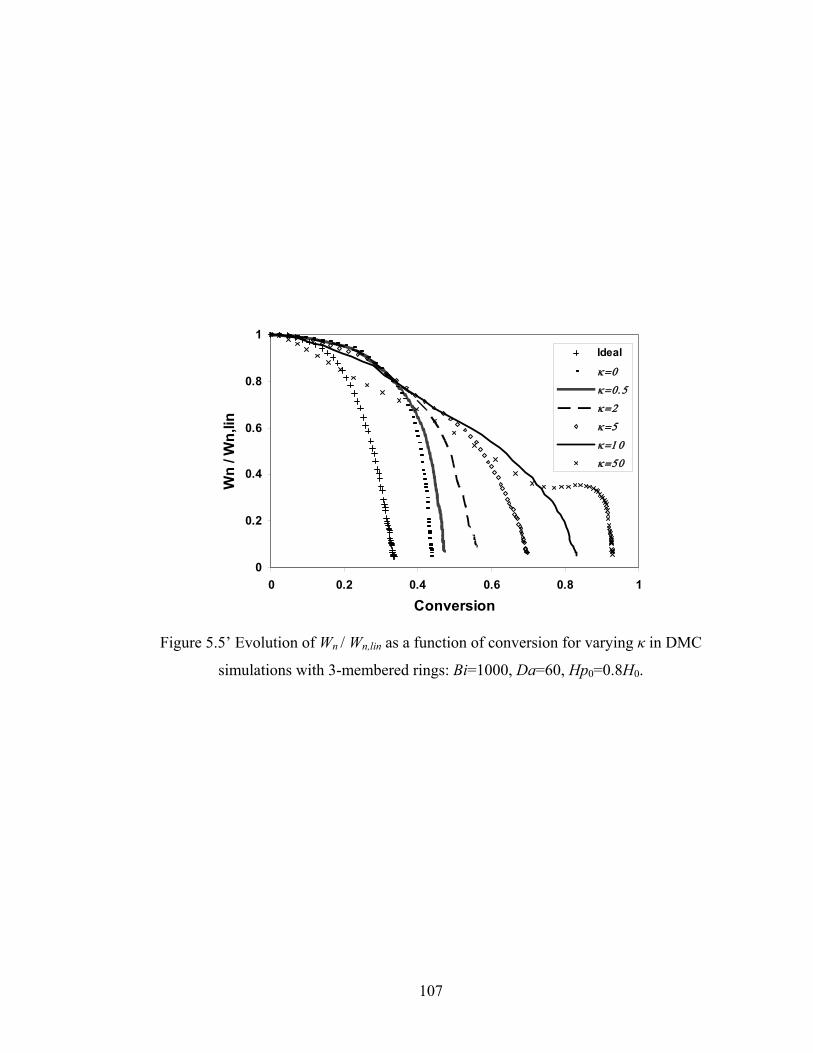
107

0

0.2

0.4

0.6

0.8

1

0 0.2 0.4 0.6 0.8 1

Conversion

Wn

/ Wn,

lin

Ideal

κ=0

κ=0.5

κ=2

κ=5

κ=10

κ=50

Figure 5.5’ Evolution of Wn / Wn,lin as a function of conversion for varying κ in DMC

simulations with 3-membered rings: Bi=1000, Da=60, Hp0=0.8H0.

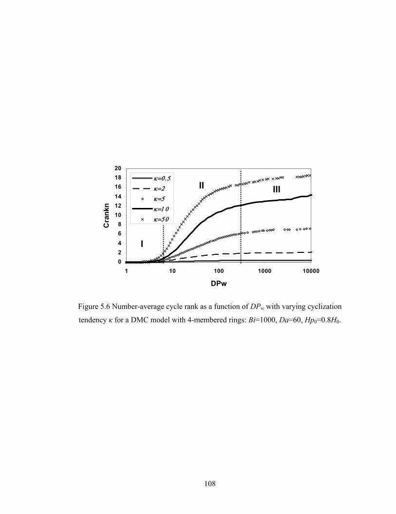
108

Figure 5.6 Number-average cycle rank as a function of DPw with varying cyclization

tendency κ for a DMC model with 4-membered rings: Bi=1000, Da=60, Hp0=0.8H0.

02468

101214161820

1 10 100 1000 10000

DPw

Cra

nkn

κ=0.5

κ=2κ=5

κ=10κ=50

I

II III

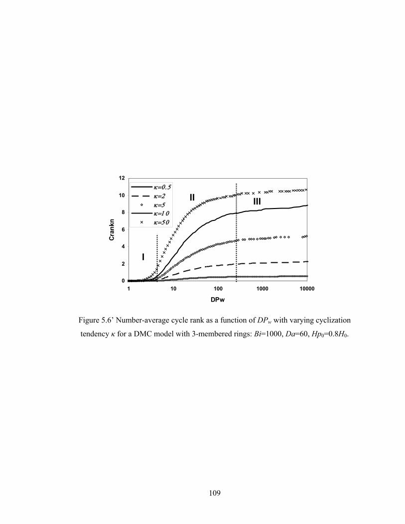
109

Figure 5.6’ Number-average cycle rank as a function of DPw with varying cyclization

tendency κ for a DMC model with 3-membered rings: Bi=1000, Da=60, Hp0=0.8H0.

0

2

4

6

8

10

12

1 10 100 1000 10000

DPw

Cran

kn

κ=0.5κ=2κ=5κ=10κ=50

I

II III

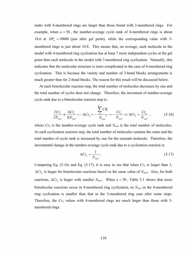
110

ranks with 4-membered rings are larger than those found with 3-membered rings. For

example, when 50=κ , the number-average cycle rank of 4-membered rings is about

18.6 at 10000=wDP (just after gel point), while the corresponding value with 3-

membered rings is just about 10.8. This means that, on average, each molecule in the

model with 4-membered ring cyclization has at least 7 more independent cycles at the gel

point than each molecule in the model with 3-membered ring cyclization. Naturally, this

indicates that the molecular structure is more complicated in the case of 4-membered ring

cyclization. This is because the variety and number of 3-bond blocks arrangements is

much greater than for 2-bond blocks. The reason for this result will be discussed below.

At each bimolecular reaction step, the total number of molecules decreases by one and

the total number of cycles does not change. Therefore, the increment of number-average

cycle rank due to a bimolecular reaction step is:

mol

nn

mol

n

mol

N

ii

nmol

n

mol

n

NCrCr

NCr

N

CRCr

NCr

NCr

mol

=⇒−=−=−=≅∂∂ ∑

= ΔΔΔΔ

21 , (5.16)

where Crn is the number-average cycle rank and Nmol is the total number of molecules.

At each cyclization reaction step, the total number of molecules remains the same and the

total number of cycle rank is increased by one for the reactant molecule. Therefore, the

incremental change in the number-average cycle rank due to a cyclization reaction is:

mol

n NCr 1Δ = , (5.17)

Comparing Eq. (5.16) and Eq. (5.17), it is easy to see that when Crn is larger than 1,

nCrΔ is larger for bimolecular reactions based on the same value of Nmol. Also, for both

reactions, nCrΔ is larger with smaller Nmol. When 50=κ , Table 5.1 shows that more

bimolecular reactions occur in 4-membered ring cyclization, so Nmol in the 4-membered

ring cyclization is smaller than that in the 3-membered ring case after some steps.

Therefore, the Crn values with 4-membered rings are much larger than those with 3-

membered rings.

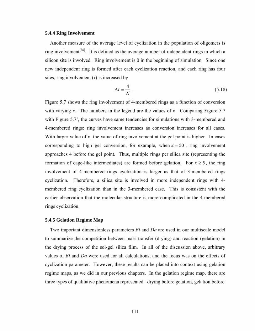
111


Another measure of the average level of cyclization in the population of oligomers is

ring involvement[38]. It is defined as the average number of independent rings in which a

silicon site is involved. Ring involvement is 0 in the beginning of simulation. Since one

new independent ring is formed after each cyclization reaction, and each ring has four

sites, ring involvement (I) is increased by

N

I 4Δ = . (5.18)

Figure 5.7 shows the ring involvement of 4-membered rings as a function of conversion

with varying κ. The numbers in the legend are the values of κ. Comparing Figure 5.7

with Figure 5.7’, the curves have same tendencies for simulations with 3-membered and

4-membered rings: ring involvement increases as conversion increases for all cases.

With larger value of κ, the value of ring involvement at the gel point is higher. In cases

corresponding to high gel conversion, for example, when 50=κ , ring involvement

approaches 4 before the gel point. Thus, multiple rings per silica site (representing the

formation of cage-like intermediates) are formed before gelation. For 5≥κ , the ring

involvement of 4-membered rings cyclization is larger as that of 3-membered rings

cyclization. Therefore, a silica site is involved in more independent rings with 4-

membered ring cyclization than in the 3-membered case. This is consistent with the

earlier observation that the molecular structure is more complicated in the 4-membered

rings cyclization.


Two important dimensionless parameters Bi and Da are used in our multiscale model

to summarize the competition between mass transfer (drying) and reaction (gelation) in

the drying process of the sol-gel silica film. In all of the discussion above, arbitrary

values of Bi and Da were used for all calculations, and the focus was on the effects of

cyclization parameter. However, these results can be placed into context using gelation

regime maps, as we did in our previous chapters. In the gelation regime map, there are

three types of qualitative phenomena represented: drying before gelation, gelation before

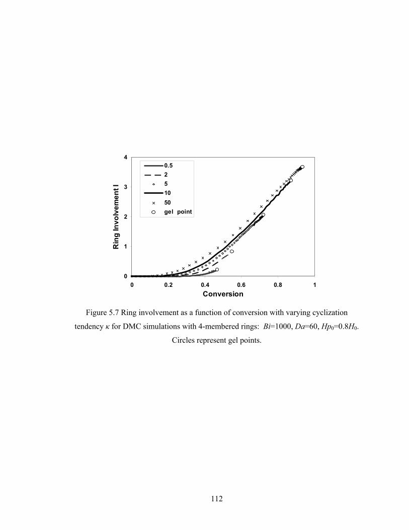
112

0

1

2

3

4

0 0.2 0.4 0.6 0.8 1Conversion

Rin

g In

volv

emen

t I

0.5251050gel point

Figure 5.7 Ring involvement as a function of conversion with varying cyclization

tendency κ for DMC simulations with 4-membered rings: Bi=1000, Da=60, Hp0=0.8H0.

Circles represent gel points.

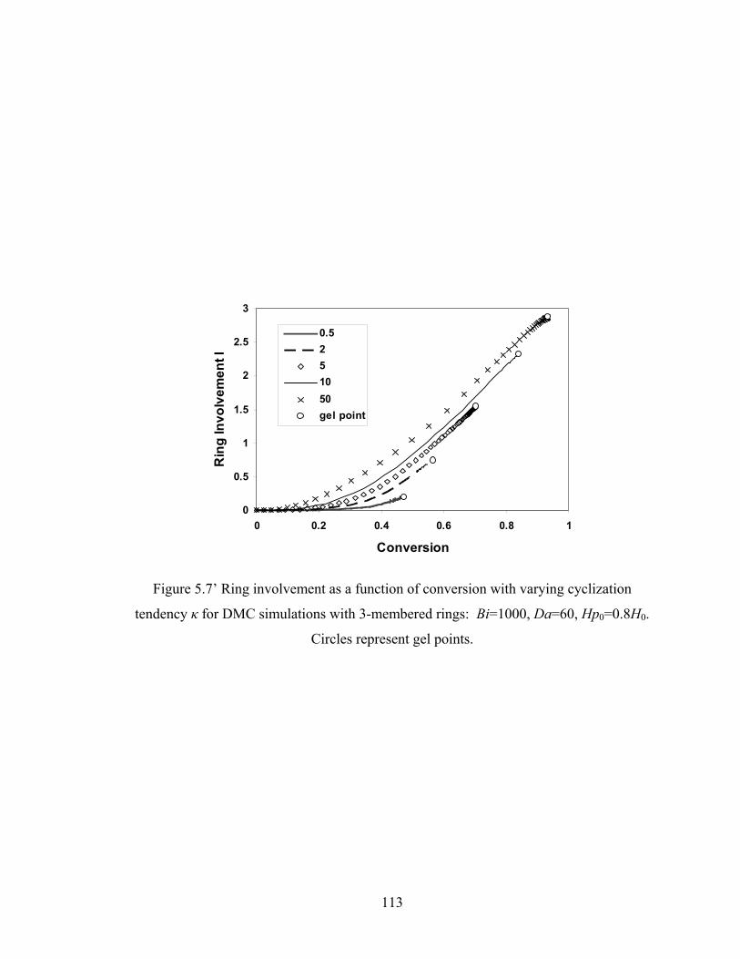
113

0

0.5

1

1.5

2

2.5

3

0 0.2 0.4 0.6 0.8 1

Conversion

Rin

g In

volv

emen

t I

0.5251050gel point

Figure 5.7’ Ring involvement as a function of conversion with varying cyclization

tendency κ for DMC simulations with 3-membered rings: Bi=1000, Da=60, Hp0=0.8H0.

Circles represent gel points.

114

drying and literal skinning[36]. These are defined based on time to dry values and gelation

times at the top and bottom of the film, and thus give a global picture of the state of the

film predicted by the multiscale DMC / continuum model. Figure 5.8 shows the gelation

regime map for simulations with unlimited 4-membered ring cyclization and with a fixed

value of 5=κ . For 4-membered rings, this is very much an experimentally relevant

value. For the cases where Ng and McCormick were able to estimate k4c(1,1) and k11 of

acid-catalyzed tetraethyl orthosilicate sol-gel solutions, the average ratio of the two has a

value of about 5.5 mol/L[52]. Therefore, if an as-deposited sol has a concentration close to

[Si]0 = 1 mol/L, this gives a value for a realistic sol-gel silica solution of κ ~ 5. Also in

terms of the modeling, this value is interesting to study because it represents the

conditions with greatest sensitivity of gel conversion difference between film surface and

base (and therefore gel structure) to concentration. Comparing Figure 5.8 with the

gelation regime map of a multiscale model with 3-membered rings (Figure 5.8’), they are

very similar and almost overlap, but the literal skinning region is subtly expanded in the

4-membered ring case.

As discussed above, one of the advantages of our multiscale model is that it allows us

to probe the microstructural implications of macroscopic transport processes. One of the

unique insights it offers is into structural gradients that can form as a result of

concentration gradients present during literal skinning. An example of the effect of 4-

membered ring cyclization on literal skinning is shown in Figure 5.9. It shows number-

average cycle rank as a function of time for different initial particle positions. The first

thing that we can notice from this figure is that according to the gel points (circles) on the

graph, the film gels much faster at the surface than inside the film. That means there is a

time lag for gelation between the film surface and base. Such time lags are characteristic

of literal skinning and are seen in all gelling / drying systems under the right conditions.

However, a new feature is also revealed – the gel points on the curves indicate what

extent of number-average cycle rank can be reached before gelation for different initial

sol particle positions. Figure 5.9 clearly shows that the number-average cycle rank at the

gel point inside the film is twice as large as it is at the film surface. Therefore, there is a

molecular structure gradient inside the film. We compare this finding with the

corresponding figure for a model with 3-membered rings in Figure 5.9’. It is clear that

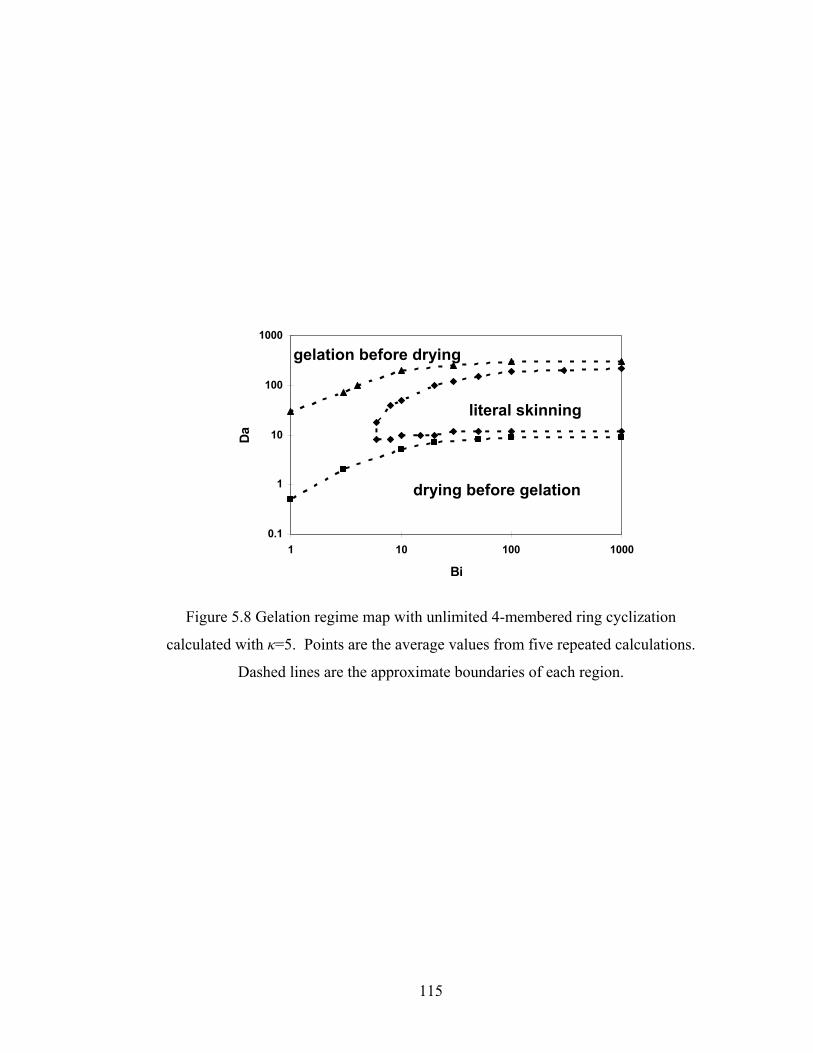
115

Figure 5.8 Gelation regime map with unlimited 4-membered ring cyclization

calculated with κ=5. Points are the average values from five repeated calculations.


0.1

1

10

100

1000

1 10 100 1000

Bi

Da



literal skinning

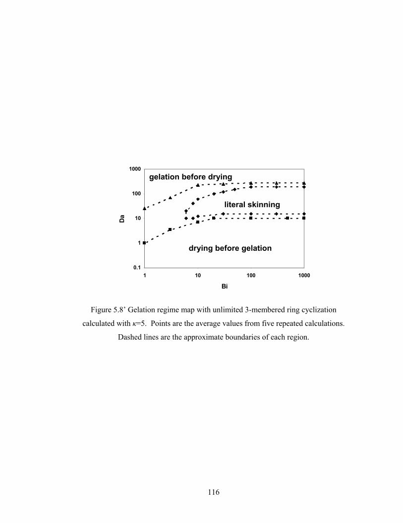
116

Figure 5.8’ Gelation regime map with unlimited 3-membered ring cyclization

calculated with κ=5. Points are the average values from five repeated calculations.


0.1

1

10

100

1000

1 10 100 1000

Bi

Da


literal skinning


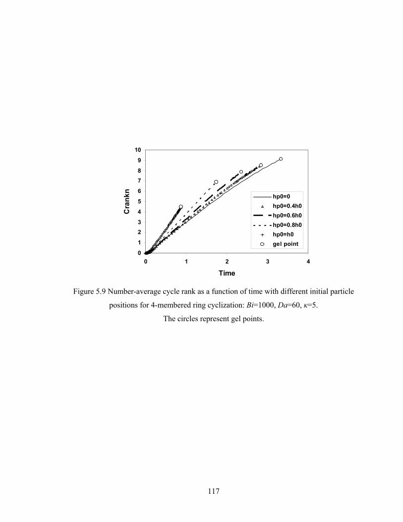
117

0

1

23

4

5

6

78

9

10

0 1 2 3 4

Time

Cra

nkn

hp0=0hp0=0.4h0hp0=0.6h0hp0=0.8h0hp0=h0gel point

Figure 5.9 Number-average cycle rank as a function of time with different initial particle

positions for 4-membered ring cyclization: Bi=1000, Da=60, κ=5.

The circles represent gel points.

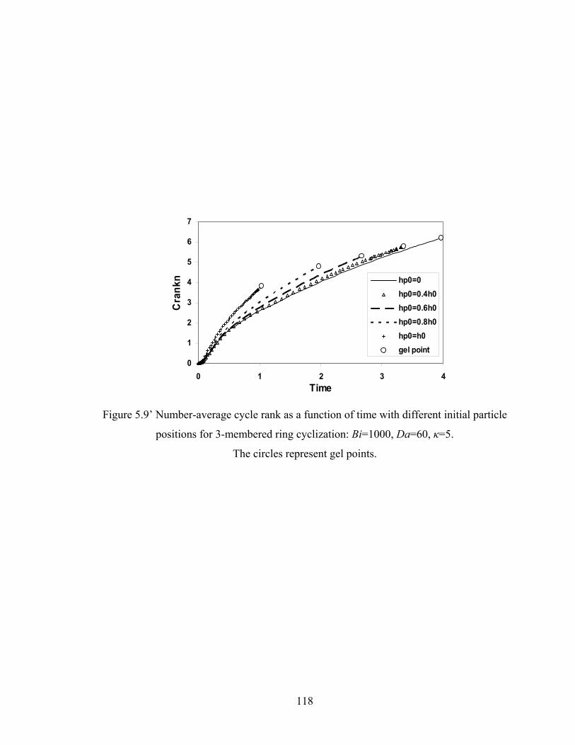
118

0

1

2

3

4

5

6

7

0 1 2 3 4Time

Cra

nkn hp0=0

hp0=0.4h0hp0=0.6h0hp0=0.8h0hp0=h0gel point

Figure 5.9’ Number-average cycle rank as a function of time with different initial particle

positions for 3-membered ring cyclization: Bi=1000, Da=60, κ=5.

The circles represent gel points.

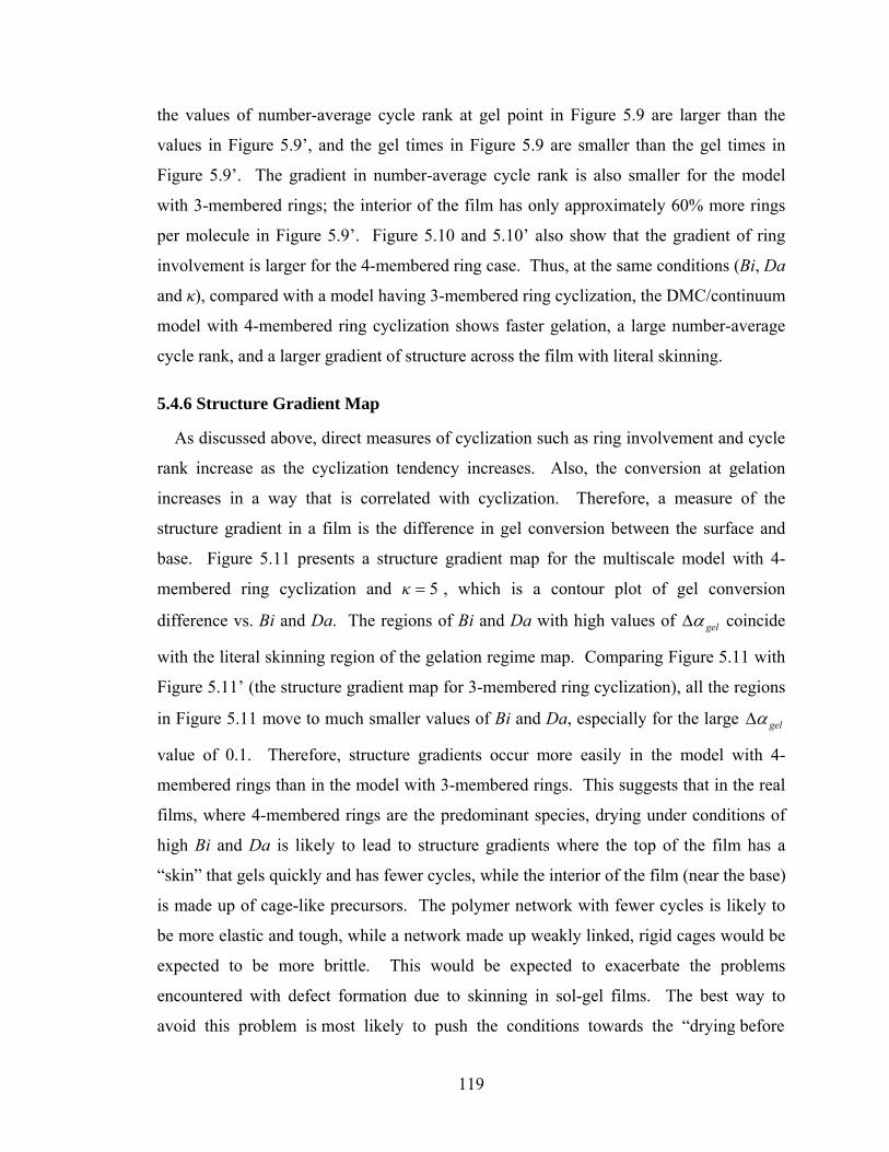
119

the values of number-average cycle rank at gel point in Figure 5.9 are larger than the

values in Figure 5.9’, and the gel times in Figure 5.9 are smaller than the gel times in

Figure 5.9’. The gradient in number-average cycle rank is also smaller for the model

with 3-membered rings; the interior of the film has only approximately 60% more rings

per molecule in Figure 5.9’. Figure 5.10 and 5.10’ also show that the gradient of ring

involvement is larger for the 4-membered ring case. Thus, at the same conditions (Bi, Da

and κ), compared with a model having 3-membered ring cyclization, the DMC/continuum

model with 4-membered ring cyclization shows faster gelation, a large number-average

cycle rank, and a larger gradient of structure across the film with literal skinning.

5.4.6 Structure Gradient Map

As discussed above, direct measures of cyclization such as ring involvement and cycle

rank increase as the cyclization tendency increases. Also, the conversion at gelation

increases in a way that is correlated with cyclization. Therefore, a measure of the

structure gradient in a film is the difference in gel conversion between the surface and

base. Figure 5.11 presents a structure gradient map for the multiscale model with 4-

membered ring cyclization and 5=κ , which is a contour plot of gel conversion

difference vs. Bi and Da. The regions of Bi and Da with high values of gelαΔ coincide

with the literal skinning region of the gelation regime map. Comparing Figure 5.11 with

Figure 5.11’ (the structure gradient map for 3-membered ring cyclization), all the regions

in Figure 5.11 move to much smaller values of Bi and Da, especially for the large gelαΔ

value of 0.1. Therefore, structure gradients occur more easily in the model with 4-

membered rings than in the model with 3-membered rings. This suggests that in the real

films, where 4-membered rings are the predominant species, drying under conditions of

high Bi and Da is likely to lead to structure gradients where the top of the film has a

“skin” that gels quickly and has fewer cycles, while the interior of the film (near the base)

is made up of cage-like precursors. The polymer network with fewer cycles is likely to

be more elastic and tough, while a network made up weakly linked, rigid cages would be

expected to be more brittle. This would be expected to exacerbate the problems

encountered with defect formation due to skinning in sol-gel films. The best way to

avoid this problem is most likely to push the conditions towards the “drying before

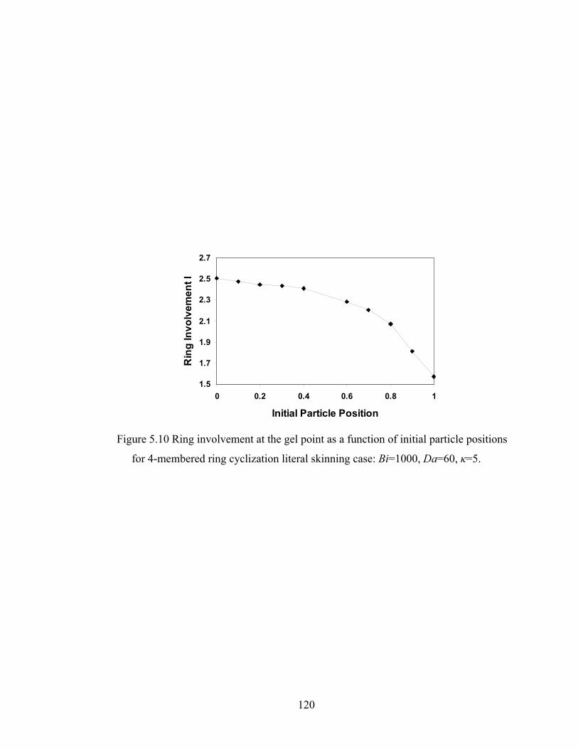
120

1.5

1.7

1.9

2.1

2.3

2.5

2.7

0 0.2 0.4 0.6 0.8 1


Rin

g In

volv

emen

t I

Figure 5.10 Ring involvement at the gel point as a function of initial particle positions

for 4-membered ring cyclization literal skinning case: Bi=1000, Da=60, κ=5.

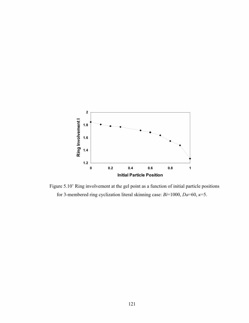
121

1.2

1.4

1.6

1.8

2

0 0.2 0.4 0.6 0.8 1


Rin

g In

volv

emen

t I

Figure 5.10’ Ring involvement at the gel point as a function of initial particle positions

for 3-membered ring cyclization literal skinning case: Bi=1000, Da=60, κ=5.

122

Figure 5.11 Structure gradient map for the 4-membered ring cyclization case with κ=5.


Dashed lines are the approximate contours of constant gelαΔ .

0

20

40

60

80

100

10 100 1000

Bi

Da

>0.04

>0.06

>0.08 >0.1

>0.12

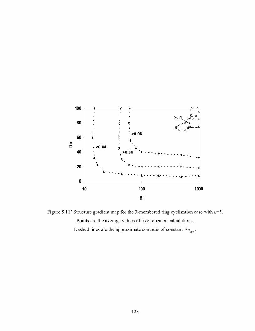
123

Figure 5.11’ Structure gradient map for the 3-membered ring cyclization case with κ=5.


Dashed lines are the approximate contours of constant gelαΔ .

0

20

40

60

80

100

10 100 1000

Bi

Da

>0.04 >0.06

>0.08

>0.1

124

gelation” regime, so that a uniform gel film without residual solvent forms.

5.5 Summary

The results of a multiscale model for the drying and curing process of sol-gel silica

films with unlimited 4-membered ring cyclization are presented. Two main links

between the parts of the multiscale model are as follows: first, in the continuum model,

the entire DMC simulation is treated as a particle of sol whose position and composition

are tracked using a diffusion / evaporation finite difference calculation. The importance

of this particle tracking is that the continuum model provides the total silicon

concentration for the DMC model, and this thus serves as a spatially distributed

“handshake” between the DMC and continuum calculations. The second “handshake”

between the models is the time interval for each bond addition in the DMC simulation,

which is used as the time interval for the finite difference calculation.

By comparing with our previous model of drying sol-gel films with unlimited 3-

membered ring cyclization, this new model allowed us to comment on a more physically

relevant type of cyclization. As in the previous model, the model with 4-membered rings

showed that the gel conversion increases as dimensionless cyclization tendency κ

increases, and for reasonable values of κ, gel conversion meeting or exceeding the

experimental value (82%) was observed. Calculations of the topological Wiener index

clearly showed that cyclization shrinks the molecular size, including in extreme cases the

formation of cage-like precursors that remain compact until the gel point.

Competition between molecular growth and cyclization can be understood using plots

of number-average cycle rank as a function of weight-average degree of polymerization.

This allows us to make a fair comparison of different cases independent of the changes in

gel time and conversion induced by cyclization. Three stages were identified based on

the plots: a growth stage where cycle rank remains low, a cyclization stage where cycle

rank increases rapidly and a gelation stage where cycle rank reaches a plateau and growth

takes off. For 5≥κ , on average, each molecule in the new model with 4-membered

rings has more independent cycles than each molecule in the former model with 3-

membered rings, indicating that the molecular structure is more complicated in the 4-

membered ring case.

125

The gelation regime map shows the competition between mass transfer (drying) and

reaction (gelation) in the coating process of the sol-gel silica films. The gelation regime

maps of models with 4-membered rings and with 3-membered rings were found to be

very similar and almost overlapped; the only difference is that the literal skinning region

of is a very slightly expanded with 4-membered rings.

The relationships between measures of cyclization (ring involvement and number-

averaged cycle rank) and conversion, time and initial particle position were investigated.

The simulations showed that cage-like intermediates form before gelation when the gel

conversion is high (with large κ). The number-average cycle rank and the ring

involvement at gel conversion inside the film are much larger than those at the surface in

many experimentally relevant conditions, so that there is a molecular structure gradient

inside the film. The gradients in number-average cycle rank and ring involvement are

smaller for the model with 3-membered rings, which also points out that the molecular

structure is more complicated in the model with 4-membered ring cyclization. At the

same conditions (Bi, Da and κ), compared with the 3-membered ring case, 4-membered

ring cyclization causes gels to form more quickly and produces gels with more rings per

molecule.

The simulations predict that high values of gel conversion difference between the

surface and base of a film coincide with the literal skinning region of the gelation regime

map. They also show that the structure gradients in the films with 4-membered rings are

larger than those found in films with 3-membered rings. The formation of gel structure

gradients would be expected to exacerbate defect formation due to literal skinning.

While its development has been complex, this multiscale model represents a first step

to understanding the complete coating process of sol-gel silica. The inclusion of

unlimited 4-membered ring cyclization will give more accurate and relevant predictions

than our previous models. Still, this model still can be improved in several aspects. For

example, transport properties were assumed to be constant during polymerization. The

multiscale model provides the opportunity for more “handshaking” between the model

components to improve this situation. One way of doing this it to utilize the Wiener

index with diffusivity correlations to provide a more physically relevant self-consistent

continuum / DMC result in the future. In addition, some limitations may need to be

126

added for the cyclization reactions, because realistic molecular structures need to be

constrained by the actual bond angles and energies of the oligomers. Although 4-

membered rings are the dominant units, there are still some 3-membered rings found in

the experiments. Therefore, a more comprehensive model would combine 3- and 4-

membered ring cyclization and would include reversibility of cyclization. This,

obviously, is a substantial challenge even with available computational resources, but

these are challenges that can be overcome in future developments.

127

Chapter 6

Conclusions

Comprehensive modeling of the coating process of sol-gel silica films requires the

consideration of multiple length and time scales ranging from molecular to macroscopic.

The formation of the film is controlled by macroscopic parameters; diffusion and mass

transport occur over micron or greater lengths scales, and define the concentration fields

within which polymerization and (if surfactants are added) self-assembly occur. At the

same time, polymerization and self-assembly processes occur which control the film

properties such as film microstructure at the molecular level. Therefore, a multiscale

model should be used to link these different length and time scale together.

The multiscale model described in this dissertation for the drying process of sol-gel

coatings couples molecular to macroscopic phenomena by combining dynamic Monte

Carlo (DMC) simulations with the finite difference method (FDM). DMC simulation is a

very good choice to model the sol-gel silica polycondensation because it can capture the

complete reaction history for a finite set of monomers, it has the flexibility to handle new

types of reactions associated with the formation of large polycyclic species and cages,

and it can simulate much larger systems and much longer times than competing

molecular approaches such as molecular dynamics. The accuracy of DMC as we have

implemented it can be verified by the good agreement between simulation results and

analytical results (based on RBT) for the ideal polycondensation case. The FDM is an

easy and intuitive numerical method to model the drying process of sol-gel silica films.

Because we use a one dimensional model to develop the multiscale approach, FDM

should provide adequate numerical accuracy and precision for the purposes of this

dissertation. In our multiscale model, the entire DMC simulation (containing at least 106

monomers) is treated as a particle of sol whose position and composition are tracked

using a diffusion / evaporation finite difference calculation. Therefore, the total silicon

concentration, which is provided by the continuum model, serves as one “handshake”

with the DMC model. The second “handshake” between the models is the time interval

from the DMC simulation, which is used as the time interval for the continuum model.

128

The validity of the multiscale model is verified by the good agreement of the

conversion evolution of DMC and continuum simulations for ideal polycondensation and

FSSE cases. With assumptions of hydrolysis pseudoequilibrium and negative FSSE for

bimolecular and cyclization reactions, our multiscale model can predict that the gel

conversion increases with increasing dimensionless cyclization tendency κ , and the gel

conversion can be equal to or larger than the experimental value (82%). Calculations of

the topological Wiener index clearly showed that cyclization shrinks the molecular size,

including in extreme cases the formation of cage-like precursors that remain compact

until the gel point.

Curves of number-average cycle rank as a function of weight-average degree of

polymerization represent the competition between molecular growth and cyclization.

This allows us to make a fair comparison of different cases independent of the changes in

gel time and conversion induced by cyclization. Three stages are obtained based on the

results: i) A growth stage in which molecular growth dominates over cyclization. ii) A

cyclization stage where cyclization increases much quicker than the first stage, and

growth is slow, especially for 5≥κ . iii) A gelation stage where growth dominates over

cyclization again until the sol-gel transition begins. For 5≥κ , on average, each

molecule in the model with 4-membered rings has more independent cycles than each

molecule in the model with 3-membered rings, indicating that the molecular structure is

more complicated in the 4-membered ring case.

The gelation regime map shows the effects of the competition between mass transfer

(drying) and reaction (gelation) on the drying process of the sol-gel silica film.

Compared with similar maps for the ideal polycondensation and FSSE cases, the

cyclization case has the same tendency to generate three types of phenomena: drying

before gelation, literal skinning and gelation before drying. The difference is that the

literal skinning region is expanded with cyclization. That means that cyclization increases

the likelihood of literal skinning.

The relationships of ring involvement and conversion, number-average cycle rank and

time with different κ values, ring involvement and initial particle position were

investigated. The simulations showed that cage-like intermediates form before gelation

at high gel conversion cases (with large κ ). With drying the maximum value of ring

129

involvement inside the film is much larger in some cases than that at the surface,

suggesting that cyclization can lead to a molecular structure gradient inside the film.

The simulations predict that high values of gel conversion difference between the

surface and base of a film coincide with the literal skinning region of the gelation regime

map. They also show that the structure gradients in the films with 4-membered rings are

larger than those found in films with 3-membered rings. The formation of gel structure

gradients would be expected to exacerbate defect formation due to literal skinning.

The dissertation presents the first multiscale model of polymerization and drying in

sol-gel films, and our model confirms the hypothesis that cyclization can lead to structure

gradients. While our multiscale model is improved from just considering FSSE to

including unlimited 3-membered ring cyclization, further to including unlimited 4-

membered ring cyclization, it represents a first step to understanding the complete

coating process of sol-gel silica. Still, this model can be improved in several aspects.

For example, some limitations may need to be added for the cyclization reactions,

because realistic molecular structures need to be constrained by the bond angles and

energies. Although 4-membered rings are the dominant units, there are still some 3-

membered rings found in the experiments. Therefore, a more comprehensive model

would combine 3- and 4-membered ring cyclization and would include reversibility of

cyclization. In addition, transport properties were assumed to be constant during

polymerization. The multiscale model provides the opportunity for more “handshaking”

between the model components to improve this situation. For example, the Wiener index

can be utilized with diffusivity correlations to provide a more physically relevant self-

consistent continuum / DMC result in the future. This, obviously, is a substantial

challenge even with available computational resources, but these are challenges that can

be overcome in future developments. The dissertation focuses on processing-structure

relationships in the films. Using structure-property relationships to understand more

about how the structure gradient influences the properties of the film is a logical

extension of our work. Another important direction of future work is to expand our 1D

model into two dimensions, using finite element method substituting finite difference

method to establish a similar connection between the DMC simulations in 2D and the

continuum calculations, as we have described in this dissertation for 1D calculations. We

130

expect that our simulation will allow better prediction of the formation of structure

gradients in sol-gel derived ceramics and other nonideal multifunctional

polycondensation products, and that this will help in developing coating procedures to

reduce coating defects in the future.

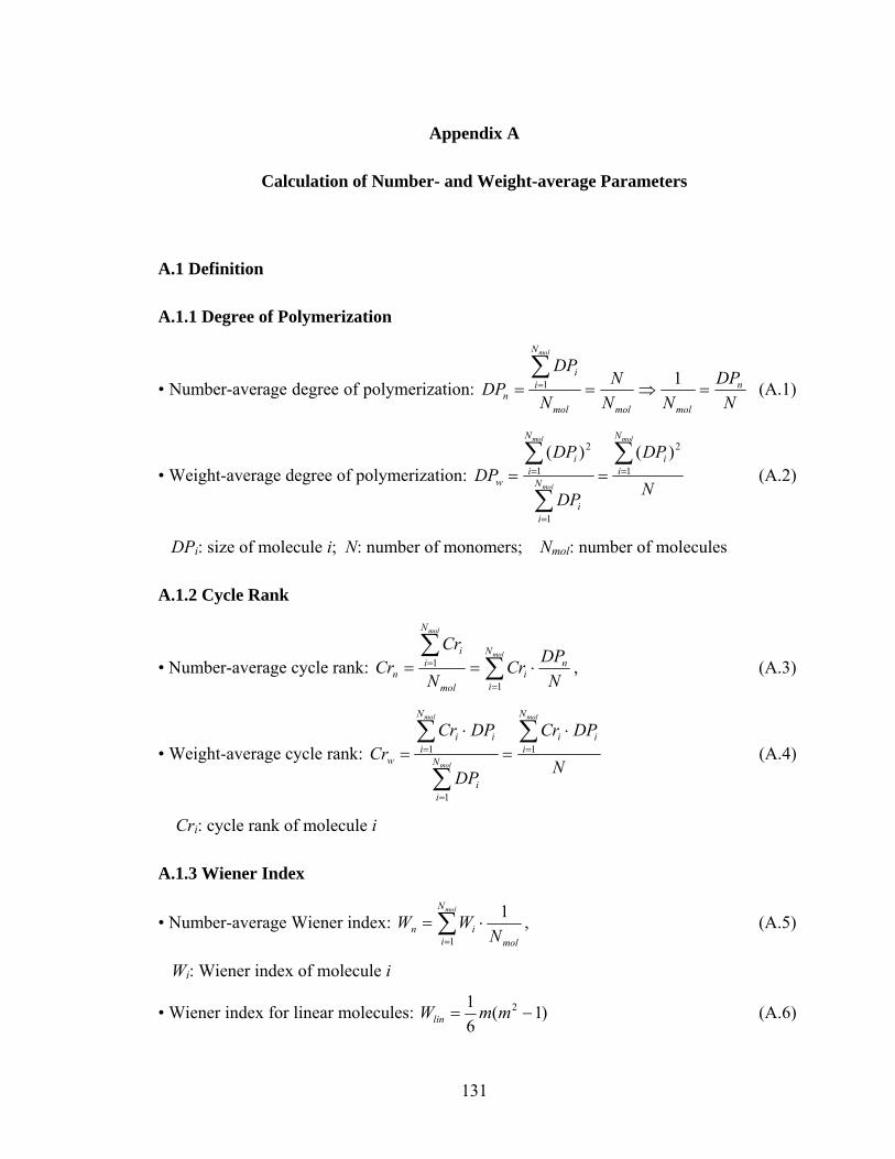
131

Appendix A

Calculation of Number- and Weight-average Parameters

A.1 Definition

A.1.1 Degree of Polymerization

• Number-average degree of polymerization: N

DPNN

NN

DPDP n

molmolmol

N

ii

n

mol

=⇒==∑= 11 (A.1)

• Weight-average degree of polymerization: N

DP

DP

DPDP

mol

mol

mol N

ii

N

ii

N

ii

w

∑

∑

∑=

=

= == 1

2

1

1

2 )()( (A.2)

DPi: size of molecule i; N: number of monomers; Nmol: number of molecules

A.1.2 Cycle Rank

• Number-average cycle rank: N

DPCrN

CrCr n

N

ii

mol

N

ii

n

mol

mol

⋅== ∑∑

=

=

1

1 , (A.3)

• Weight-average cycle rank: N

DPCr

DP

DPCrCr

mol

mol

mol N

iii

N

ii

N

iii

w

∑

∑

∑=

=

=

⋅=

⋅= 1

1

1 (A.4)

Cri: cycle rank of molecule i

A.1.3 Wiener Index

• Number-average Wiener index: mol

N

iin N

WWmol 11

⋅= ∑=

, (A.5)

Wi: Wiener index of molecule i

• Wiener index for linear molecules: )1(61 2 −= mmWlin (A.6)

132

m: molecular size

A.2 Bimolecular Condensation Reactions

After each bimolecular reaction, the number of molecules is decreased by 1, i.e.

1Δ −=chainsN . Assuming the bimolecular reaction occurs between molecule i (size m) and

j (size n):

A.2.1 Degree of Polymerization

• Number-average degree of polymerization:

∵ nmol

n

mol

n DPNDP

NDP Δ

ΔΔ

−=≅∂∂ , and

NDP

NN

N

DP

NNDP n

molmol

N

ii

molmol

n

mol

2

21

)()( −=−=

∂∂

=∂∂ ∑

=

∴ N

DPDP nn

2

Δ = (A.7)

• Weight-average degree of polymerization:

∵ NDPDPDP ji

beforew)( 22

_++++

= ,

NDPDPDPDP

NDPDPDP jjiiji

afterw)2())(( 222

_++⋅⋅++

=+++

=

∴ NDPDPDPDPDP ji

beforewafterww⋅⋅

=−=2Δ __ (A.8)

A.2.2 Cycle Rank

• Number-average cycle rank:

∵ nmol

n

mol

n CrNCr

NCr Δ

ΔΔ

−=≅∂∂ , and

NDPCr

NCr

N

Cr

NCr nn

mol

n

mol

N

ii

mol

n

mol

⋅−=−=−=

∂∂ ∑

=2

1

)(

∴ N

DPCrCr nnn

⋅=Δ (A.9)

• Weight-average cycle rank:

∵ NDPCrDPCrCr jjii

beforew)(

_+⋅++⋅+

=

NDPDPCrCrCr jiji

afterw))()((

_++⋅++

=

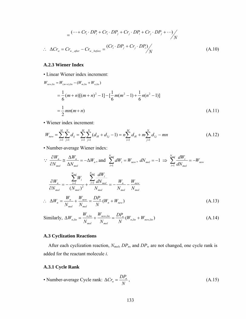
133

NDPCrDPCrDPCrDPCr jjijjiii )( +⋅+⋅+⋅+⋅+

=

∴ NDPCrDPCrCrCrCr ijji

beforewafterww)(Δ __

⋅+⋅=−= (A.10)

A.2.3 Wiener Index

• Linear Wiener index increment:

)( ,,),(, linnlinmlinnmlinnew WWWW +−= +

)]1(61)1(

61[]1))[((

61 222 −+−−−++= nnmmnmnm

)(21 nmmn += (A.11)

• Wiener index increment:

∑∑∑∑= == =

−+==M

i

N

jLjiR

M

i

N

jijnew dddW

1 11 1)1( mndmdn

N

jLj

M

iiR −+= ∑∑

== 11 (A.12)

• Number-average Wiener index:

∵ nmol

n

mol

n WNW

NW Δ

ΔΔ

−=≅∂∂ , and new

N

ii WdW

mol

=∑=1

, 1−=moldN ⇒ ∑=

−=molN

inew

mol

i WdNdW

1

mol

new

mol

n

mol

N

i mol

i

mol

N

ii

mol

n

NW

NW

NdNdW

N

W

NW

molmol

−−=+−=∂∂ ∑∑

== 12

1

)(

∴ )(Δ newnn

mol

new

mol

nn WW

NDP

NW

NWW +=+= (A.13)

Similarly, )(Δ ,,,,

, linnewlinnn

mol

linnew

mol

linnlinn WW

NDP

NW

NW

W +=+= (A.14)

A.3 Cyclization Reactions

After each cyclization reaction, Nmol, DPn, and DPw are not changed, one cycle rank is

added for the reactant molecule i.

A.3.1 Cycle Rank

• Number-average Cycle rank: N

DPCr nn =Δ , (A.15)

134

• Weight-average Cycle rank: NDPCr i

w =Δ (A.16)

A.3.2 Wiener Index

• Number-average Wiener index: N

DPWNWW nnew

mol

newn

⋅==Δ (A.17)

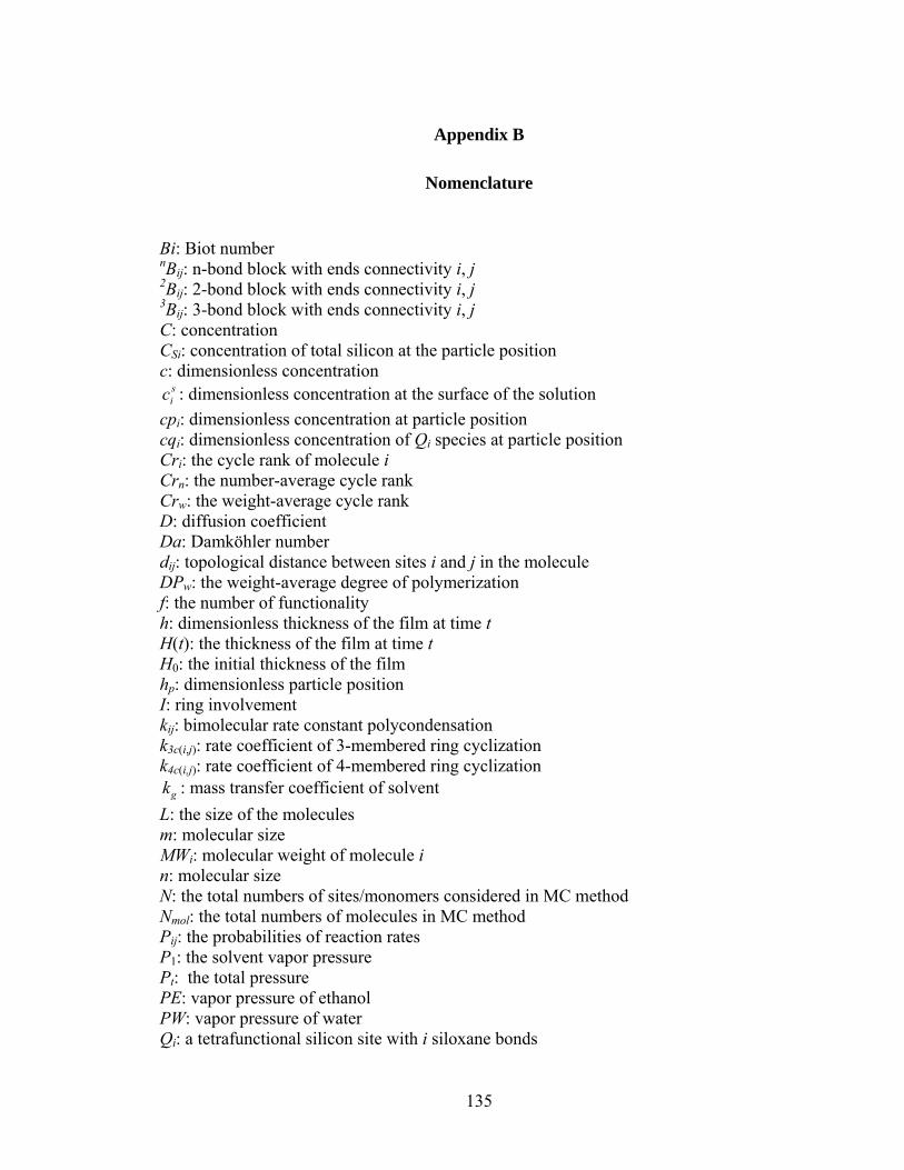
135

Appendix B

Nomenclature

Bi: Biot number nBij: n-bond block with ends connectivity i, j 2Bij: 2-bond block with ends connectivity i, j 3Bij: 3-bond block with ends connectivity i, j C: concentration CSi: concentration of total silicon at the particle position c: dimensionless concentration

sic : dimensionless concentration at the surface of the solution

cpi: dimensionless concentration at particle position cqi: dimensionless concentration of Qi species at particle position Cri: the cycle rank of molecule i Crn: the number-average cycle rank Crw: the weight-average cycle rank D: diffusion coefficient Da: Damköhler number dij: topological distance between sites i and j in the molecule

DPw: the weight-average degree of polymerization f: the number of functionality h: dimensionless thickness of the film at time t H(t): the thickness of the film at time t H0: the initial thickness of the film hp: dimensionless particle position I: ring involvement kij: bimolecular rate constant polycondensation k3c(i,j): rate coefficient of 3-membered ring cyclization k4c(i,j): rate coefficient of 4-membered ring cyclization

gk : mass transfer coefficient of solvent L: the size of the molecules m: molecular size MWi: molecular weight of molecule i n: molecular size N: the total numbers of sites/monomers considered in MC method Nmol: the total numbers of molecules in MC method Pij: the probabilities of reaction rates P1: the solvent vapor pressure Pt: the total pressure PE: vapor pressure of ethanol PW: vapor pressure of water Qi: a tetrafunctional silicon site with i siloxane bonds

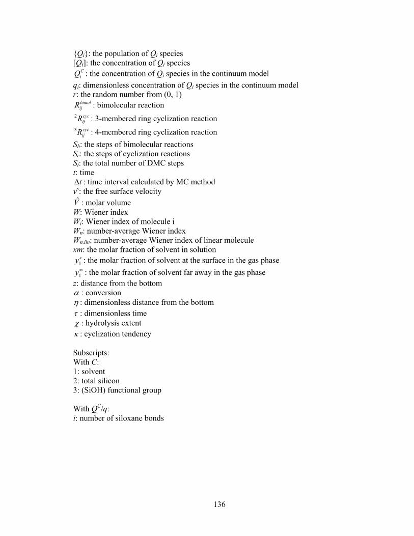
136

Qi: the population of Qi species [Qi]: the concentration of Qi species

CiQ : the concentration of Qi species in the continuum model

qi: dimensionless concentration of Qi species in the continuum model r: the random number from (0, 1)

bimolijR : bimolecular reaction

cycijR2 : 3-membered ring cyclization reaction cycijR3 : 4-membered ring cyclization reaction

Sb: the steps of bimolecular reactions Sc: the steps of cyclization reactions St: the total number of DMC steps t: time

tΔ : time interval calculated by MC method vs: the free surface velocity V : molar volume W: Wiener index Wi: Wiener index of molecule i Wn: number-average Wiener index Wn,lin: number-average Wiener index of linear molecule xm: the molar fraction of solvent in solution

sy1 : the molar fraction of solvent at the surface in the gas phase ∞1y : the molar fraction of solvent far away in the gas phase

z: distance from the bottom α : conversion η : dimensionless distance from the bottom τ : dimensionless time χ : hydrolysis extent κ : cyclization tendency Subscripts: With C: 1: solvent 2: total silicon 3: (SiOH) functional group With QC/q: i: number of siloxane bonds

137

References: 1. Sanchez, C., et al., Design, Synthesis, and Properties of Inorganic and Hybrid

Thin Films Having Periodically Organized Nanoporosity. Chem. Mater., 2008. 20(3): p. 715-720.

2. Stein, A., B.J. Melde, and R.C. Schroden, Hybrid Inorganic-Organic Mesoporous Silicates-Nanoscopic Reactors Coming of Age. Adv. Mater, 2000. 12(19): p. 1412-1417.

3. Kambhampati, D.K., et al., Novel silicon dioxide sol-gel films for potential sensor applications: A surface plasmon resonance study. Langmuir, 2001. 17(4): p. 1169-1175.

4. Anitha, K., S.V. Mohan, and S.J. Reddy, Development of acetylcholinesterase silica sol-gel immobilized biosensor. An application towards oxydemeton methyl detection. Biosens. Bioelectron., 2004. 20(4): p. 848-56.

5. Martucci, A., et al., Nanostructured sol-gel silica thin films doped with NiO and SnO2 for gas sensing applications. J. Mater. Chem., 2004. 14(19): p. 2889-2895.

6. Buso, D., et al., Porous sol gel silica films doped with crystalline NiO nanoparticles for gas sensing applications. J. Sol-Gel Sci. Technol., 2006. 40(2/3): p. 299-308.

7. Palaniappan, A., X. Su, and F.E.H. Tay, Functionalized mesoporous silica films for gas sensing applications. J. Electroceram., 2006. 16(4): p. 503-505.

8. Di, J., et al., Direct electrochemistry of lactate dehydrogenase immobilized on silica sol-gel modified gold electrode and its application. Biosens. Bioelectron., 2007. 23(5): p. 682-687.

9. Musat, V., et al., Sol-gel cobalt oxide-silica nanocomposite thin films for gas sensing applications. Thin Solid Films, 2008. 516(7): p. 1499-1502.

10. Konjhodzic, D., H. Bretinger, and F. Marlow, Structure and properties of low-n mesoporous silica films for optical applications. Thin Solid Films, 2006. 495(1-2): p. 333-337.

11. Teyssier, J., et al., LiIO3/SiO2 nanocomposite for quadratic non-linear optical applications. J. Non-Cryst. Solids, 2004. 341(1-3): p. 152-156.

12. Molenkamp, W.C., et al., Highly Polarized Luminescence from Optical Quality Films of a Semiconducting Polymer Aligned within Oriented Mesoporous Silica. J. AM. CHEM. SOC., 2004. 126: p. 4476-7.

13. Blanc, D., et al., Synthesis and characterisation of tantalum-incorporating silica hybrid sol-gel thin films for optical applications. Opt. Mater. (Amsterdam, Neth.), 2006. 28(4): p. 331-335.

14. Syms, R.R.A., et al., Development of the SC-RTA Process for Fabrication of Sol-Gel Based Silica-on-Silicon Integrated Optic Components. Journal of Sol-Gel Science and Technology, 1998. 13: p. 509-516.

15. Brusatin, G., et al., Materials for Photonic Applications From Sol-Gel. Journal of Electroceramics, 2000. 4(1): p. 151-165.

16. Olding, T., M. Sayer, and D. Barrow, Ceramic sol-gel composite coatings for electrical insulation. Thin Solid Films, 2001. 398-399: p. 581-586.

138

17. Jain, T.K., et al., Nanometer Silica Particles Encapsulating Active Compounds: A Novel Ceramic Drug Carrier. J. AM. CHEM. SOC., 1998. 120(43): p. 11092-11095.

18. Nostell, P., A. Roos, and B. Karlsson, Optical and mechanical properties of sol-gel antireflective films for solar energy applications. Thin Solid Films, 1999. 351(1,2): p. 170-175.

19. Brinker, C.J., et al., Sol-gel derived ceramic films - fundamentals and applications. Metallurgical and Ceramic Protective Coatings, ed. K.H. Stern. 1996: Chapman & Hall. 112-151.

20. Brinker, C.J. and A.J. Hurd, Fundamentals of sol-gel dip-coating. J. Phys. III France, 1994. 4: p. 1231-1242.

21. Lou, Y. and P.D. Christofides, Feedback control of growth rate and surface roughness in thin film growth. AIChE J., 2003. 49(8): p. 2099-2113.

22. Cairncross, R.A., L.F. Francis, and L.E. Scriven, Competing drying and reaction mechnisms in the formation of sol-to-gel films, fibers, and spheres. Drying Technology, 1992. 10(4): p. 893-923.

23. Kay, B.D. and R.A. Assink, Sol-gel kinetics. II. Chemical speciation modeling. J. Non-Cryst. Solids, 1988. 104(1): p. 112-22.

24. Assink, R.A. and B.D. Kay, Sol-gel kinetics. I. Functional group kinetics. J. Non-Cryst. Solids, 1988. 99(2-3): p. 359-70.

25. Sanchez, J. and A.V. McCormick, Kinetic and thermodynamic study of the hydrolysis of silicon alkoxides in acidic alcohol solutions. J. Phys. Chem., 1992. 96(22): p. 8973-9.

26. Alam, T.M., R.A. Assink, and D.A. Loy, Hydrolysis and Esterification in Organically Modified Alkoxysilanes: A 29Si NMR Investigation of Methyltrimethoxysilane. Chem. Mater., 1996. 8(9): p. 2366-74.

27. Rankin, S.E., C.W. Macosko, and A.V. McCormick, Sol-gel polycondensation kinetic modeling: methylethoxysilanes. AIChE J., 1998. 44(5): p. 1141-1156.

28. Rankin, S.E. and A.V. McCormick, Hydrolysis pseudoequilibrium: challenges and opportunities to sol-gel silicate kinetics. Chem. Eng. Sci., 2000. 55(11): p. 1955-1967.

29. Rankin, S.E., J. Šefčίk, and A.V. McCormick, Similarities in the Hydrolysis Pseudoequilibrium Behavior of Methyl-Substituted Ethoxysilanes. Ind. Eng. Chem. Res., 1999. 38(9): p. 3191-3198.

30. Sanchez, J., S.E. Rankin, and A.V. McCormick, 29Si NMR kinetic study of tetraethoxysilane and ethyl-substituted ethoxysilane polymerization in acidic conditions. Ind. Eng. Chem. Res., 1996. 35(1): p. 117-29.

31. Bailey, J.K., C.W. Macosko, and M.L. Mecartney, Modeling the gelation of silicon alkoxides. J. Non-Cryst. Solids, 1990. 125(3): p. 208-23.

32. Pouxviel, J.C. and J.P. Boilot, Kinetic simulations and mechanisms of the sol-gel polymerization J. Non-Cryst. Solids, 1987. 94(3): p. 374-86.

33. Assink, R.A. and B.D. Kay, Sol-gel kinetics. III. Test of the statistical reaction model. J. Non-Cryst. Solids, 1988. 107(1): p. 35-40.

34. Brunet, F. and B. Cabane, Populations of oligomers in sol-gel condensation. J. Non-Cryst. Solids, 1993. 163(3): p. 211-25.

139

35. Hendrickson, R.C., A.M. Gupta, and C.W. Macosko, Sol-Gel polymerization: Monte Carlo simulation of substitution effects. Comput. Polym. Sci., 1994. 4(3 & 4): p. 53-65.

36. Cairncross, R.A., L.F. Francis, and L.E. Scriven, Predicting drying in coatings that react and gel: drying regime maps. AIChE J., 1996. 42(1): p. 55-67.

37. Assink, R.A. and B.D. Kay, The chemical kinetics of silicate sol-gels: functional group kinetics of tetraethoxysilane. Colloids Surf., A, 1993. 74(1): p. 1-5.

38. Rankin, S.E., et al., Dynamic Monte Carlo Simulation of Gelation with Extensive Cyclization. Macromolecules, 2000. 33(20): p. 7639-7648.

39. Kasehagen, L.J., et al., Modeling of First Shell Substitution Effects and Preferred Cyclization in Sol-Gel Polymerization. Macromolecules, 1997. 30(13): p. 3921-3929.

40. West, J.K., et al., Quantum chemistry of sol-gel silica clusters. J. Non-Cryst. Solids, 1990. 121(1-3): p. 51-5.

41. Tang, A., et al., Characterisation of Polymeic Reaction in Silicic Acid Solution: Intramolecular Cyclization. J. Mater. Chem., 1993. 3(8): p. 893-6.

42. Sanchez, J. and A.V. McCormick, Intramolecular vs. intermolecular condensation rates in the acidic polymerization of octaethoxytrisiloxane. J. Non-Cryst. Solids, 1994. 167(3): p. 289-94.

43. Ng, L.V., et al., Formation of Cagelike Intermediates from Nonrandom Cyclization during Acid-Catalyzed Sol-Gel Polymerization of Tetraethyl Orthosilicate. Macromolecules, 1995. 28(19): p. 6471-6.

44. Vainrub, A., et al., Sol-gel polymerization in alkoxysilanes: 29Si NMR study and simulation of chemical kinetics. Mater. Sci. Eng., B, 1996. B37(1-3): p. 197-200.

45. Malier, L., et al., Nuclear-magnetic-resonance study of silica gelation kinetics. Phys. Rev. A, 1992. 46(2): p. 959-62.

46. Brunet, F., Polymerization reactions in methyltriethoxysilane studied through 29Si NMR with polarization transfer. J. Non-Cryst. Solids, 1998. 231(1,2): p. 58-77.

47. Capozzi, C.A., L.D. Pye, and R.A. Condrate, Sr., Vibrational spectral/structural changes from the hydrolysis/polycondensation of methyl-modified silicates. I. Comparisons for single monomer condensates. Mater. Lett., 1992. 15(1-2): p. 130-6.

48. Earley, C.W., A Quantum Mechanical Investigation of Silsesquioxane Cages. J. Phys. Chem., 1994. 98(35): p. 8693-8.

49. Kamiya, K., et al., X-ray diffraction of silica gels made by sol-gel method under different conditions. J. Non-Cryst. Solids, 1998. 240(1-3): p. 202-211.

50. Kelts, L.W. and N.J. Armstrong, A silicon-29 NMR study of the structural intermediates in low pH sol-gel reactions. J. Mater. Res., 1989. 4(2): p. 423-33.

51. Klemperer, W.G., et al., Structural characterization of polysilicate intermediates formed during sol-gel polymerization. Mater. Res. Soc. Symp. Proc., 1988. 121(Better Ceram. Chem. 3): p. 15-24.

52. Ng, L.V. and A.V. McCormick, Acidic Sol-Gel Polymerization of TEOS: Effect of Solution Composition on Cyclization and Bimolecular Condensation Rates. J. Phys. Chem., 1996. 100(30): p. 12517-12531.

140

53. Tallant, D.R., et al., Raman spectra of rings in silicate materials. Mater. Res. Soc. Symp. Proc., 1986. 73(Better Ceram. Chem. 2): p. 261-7.

54. Van Beek, J.J., D. Seykens, and J.B.H. Jansen, Silicon-29 NMR monitoring and kinetic modeling of an acid-catalyzed TMOS sol-gel system with molar water/silicon = 8. J. Non-Cryst. Solids, 1992. 146(2-3): p. 111-20.

55. Wada, M., K. Kamiya, and H. Nasu, X-ray diffraction analysis of silica gel prepared from monomethyl-tri-ethoxysilane by the sol-gel method. Phys. Chem. Glasses, 1992. 33(2): p. 56-60.

56. Wada, M., et al., Structure analysis of sol-gel-derived silica gels by neutron diffraction. J. Non-Cryst. Solids, 1992. 149(3): p. 203-8.

57. Eckhardt, R., Stan Ulam, John von Neumann, and the Monte Carlo Method. LOS ALAMOS SCIENCE: Special Issue, Stanislaw Ulam 1909-1984, 1987. 15: p. 131-7.

58. Bauer, W.F., The Monte Carlo Method. Journal of the Society for Industrial and Applied Mathematics, 1958. 6(4): p. 438-51.

59. Halton, J.H., A Retrospective and Prospective Survey of the Monte Carlo Method. SIAM Review, 1970. 12(1): p. 1-63.

60. Hammersley, J.M. and D.C. Handscomb, Monte Carlo Methods, ed. M.S. Bartlett. 1964, London & New York: Chapman and Hall. 1-9.

61. Šomvársky, J. and K. Dušek, Kinetic Monte-Carlo simulation of network formation I. Simulation method. Polymer Bulletin, 1994. 33: p. 369-76.

62. Gillespie, D.T., A general method for numerically simulating the stochastic time evolution of coupled chemical reactions. J. Comput. Phys., 1976. 22(4): p. 403-34.

63. Vlachos, D.G., Instabilities in homogenwous nonisothermal reactors: Comparison of deterministic and Monte Carlo simulations. J. Chem. Phys., 1995. 102(4): p. 1781-90.

64. Šomvársky, J. and K. Dušek, Kinetic Monte-Carlo simulation of network formation II. Effect of system size. Polymer Bulletin, 1994. 33: p. 377-84.

65. Hendrickson, R., A. Gupta, and C.W. Macosko, Monte Carlo simulation of cyclization during stepwise polymerization. Comput. Polym. Sci., 1995. 5(3): p. 135-42.

66. Rankin, S.E., C.W. Macosko, and A.V. McCormick, Importance of Cyclization during the Condensation of Hydrolyzed Alkoxysilanes. Chem. Mater., 1998. 10(8): p. 2037-2040.

67. Garofalini, S.H. and G. Martin, Molecular Simulations of the Polymerization of Silicic Acid Molecules and Network Formation. J. Phys. Chem., 1994. 98(4): p. 1311-16.

68. Martin, G.E. and S.H. Garofalini, Sol-gel polymerization: analysis of molecular mechanisms and the effect of hydrogen. Journal of Non-Crystalline Solids, 1994. 171: p. 68-79.

69. Yamahara, K. and K. Okazaki, Molecular dynamics simulation of the structural development in sol-gel process for silica systems. Fluid Phase Equilibria, 1998. 144: p. 449-459.

70. Fichthorn, K.A. and W.H. Weinberg, Theoretical foundations of dynamical Monte Carlo simulations. J. Chem. Phys., 1991. 95(2): p. 1090-6.

141

71. Flory, P.J., Molecular Size Distribution in Three Dimensional Polymers. . J. AM. CHEM. SOC., 1941. 63(11): p. 3083, 3091, 3096.

72. Stockmayer, W.H., Theory of Molecular Size Distribution and gel Formation in Branched-Chain Polymers. J. Chem. Phys., 1943. 11(2): p. 45-55.

73. Stockmayer, W.H., Theory of Molecular Size Distribution and Gel Formation in Branched Polymers II. General Cross Linking. J. Chem. Phys., 1944. 12(4): p. 125-31.

74. Shy, L.Y., V.K. Leung, and B.E. Eichinger, Critical Exponents for Off-Lattice Gelation of Polymer Chains. Macromolecules, 1985. 18: p. 983-986.

75. Šefčίk, J. and S.E. Rankin, Monte Carlo simulations of size and structure of gel precursors in silica polycondensation. J. Phys. Chem. B, 2003. 107(1): p. 52-60.

76. Blandin, H.P., et al., Modelling of drying of coatings: effect of the thickness, temperature and concentration of solvent. Prog. Org. Coat., 1987. 15(2): p. 163-72.

77. Vrentas, J.S. and C.M. Vrentas, Drying of solvent-coated polymer films. J. Polym. Sci., Part B: Polym. Phys., 1994. 32(1): p. 187-94.

78. Alsoy, S. and J.L. Duda, Drying of solvent coated polymer films. Drying Technol., 1998. 16(1 & 2): p. 15-44.

79. Kuznetsov, A.V. and M. Xiong, Effect of evaporation on thin film deposition in dip coating process. Int. Comm. Heat Mass Transfer, 2002. 29(1): p. 35-44.

80. Lou, H.H. and Y.L. Huang, Integrated Modeling and Simulation for Improved Reactive Drying of Clearcoat. Ind. Eng. Chem. Res., 2000. 39(2): p. 500-507.

81. Cerro, R.L. and L.E. Scriven, Rapid free surface film flows. An integral approach. Ind. Eng. Chem. Fundam., 1980. 19(1): p. 40-50.

82. Cairncross, R.A., Modeling drying during low-speed coating of porous and continuous films. IS&T's Annu. Conf., 1997. 50th: p. 554-558.

83. Verros, G.D. and N.A. Malamataris, Finite Element Analysis of Polymeric Membrane and Coating Formation by Solvent Evaporation. Computational Mechanics, 2001. 27: p. 332-40.

84. Réglat, O., R. Labrie, and P.A. Tanguy, A new free surface model for the dip coating process. J. Comput. Phys., 1993. 109(2): p. 238-46.

85. Christodoulou, K.N., E.J. Lightfood, and R.W. Powell, Model of stress-induced defect formation in drying polymer films. AIChE Journal, 1998. 44(7): p. 1484-98.

86. LeVeque, R.J., Finite Difference Methods for Ordinary and Partial Differential Equations: Steady-State and Time-Dependent Problems. 2007, Philadalphia: Society for Industrial and Applied Mathematics.

87. Scannapieco, E. and F.H. Harlow, Introduction to Finite Difference Methods for Numerical Fluid Dynamics, in Los Alamos National Lab Report P.W. Mendius, Editor. 1995, Los Alamos National Lab: Los Alamos, New Mexico.

88. Guerrier, B., et al., Drying kinetics of polymer films. AIChE J., 1998. 44(4): p. 791-8.

89. Crank, J., Free and Moving Boundary Problems. 1988: Clarendon Press, Oxford. 90. Forsman, W.C., Graph theory and the statistics and dynamics of polymer chains.

J. Chem. Phys., 1976. 65(10): p. 4111-15. 91. Nitta, K.-h., A topological approach to statistics and dynamics of chain molecules.

J. Chem. Phys., 1994. 101(5): p. 4222-8.

142

92. Ivanciuc, O., QSAR comparative study of Wiener descriptors for weighted molecular graphs. J. Chem. Inf. Comput. Sci., 2000. 40: p. 1412-1422.

93. Ivanciuc, O., et al., Wiener index extension by counting even/odd graph distances. J. Chem. Inf. Comput. Sci., 2001. 41(3): p. 536-549.

94. Bonchev, D. and N. Trinajstić, Information theory, distance matrix, and molecular branching. J. Chem. Phys., 1977. 67(10): p. 4517-4533

95. Bersohn, M., A fast algorithm for calculation of the distance matrix of a molecule. J. Comput. Chem., 1983. 4(1): p. 110-13.

96. Müeller, W.R., et al., An algorithm for construction of the molecular distance matrix. J. Comput. Chem., 1987. 8(2): p. 170-3.

97. Cruz, R.N. and K.A. De Rezende, Cycle rank of lyapunov graphs and the genera of manifolds. American Mathematical Society, 1998. 126(12): p. 3715-3720.

98. Olemskoia, A.I. and I. Krakovský, Two simple approaches to sol–gel transition. Physica A: Statistical Mechanics and its Applications, 2001. 291(1-4): p. 79-88.

99. Guliants, V.V., M.A. Carreon, and Y.S. Lin, Ordered mesoporous and macroporous inorganic films and membranes. J. Membr. Sci., 2004. 235(1-2): p. 53-72.

100. Brinker, C.J. and D.R. Dunphy, Morphological control of surfactant-templated metal oxide films. Current Opinion in Colloid & Interface Science, 2006. 11(2,3): p. 126-132.

101. Sarmoria, C. and D.R. Miller, Spanning-tree models for Af homopolymerizations with intramolecular reactions. Comp. Theor. Polym Sci., 2001. 11: p. 113-127.

143

Vita

Born: 12/15/1976, Liancheng, Fujian, China

Education:

B.S., Chemical Engineering, East China University of Science and Technology, Shanghai,

China, July 2000.

M.S., Chemical Engineering, East China University of Science and Technology,

Shanghai, China, July 2003.

Presentations:

• Xin Li, Stephen E. Rankin. Multiscale modeling of cyclization effects in drying sol-gel

silica films, AIChE 2007 Annual Meeting, Salt Lake City, UT, November 2007.

• Xin Li, Stephen E. Rankin. Multiscale modeling of coupled drying and nonideal

polymerization in sol-gel silica films, AIChE 2006 Annual Meeting, San Francisco, CA,

November 2006.

Peer-viewed Publications:

1) Xin Li, Stephen E. Rankin. Multiscale Dynamic Monte Carlo / Continuum Modeling

of Drying and Curing in Sol-gel Silica Films (in preparation).

2) Xin Li, Stephen E. Rankin. Multiscale Modeling of Coupled Drying and Curing of

Sol-gel Silica Films with Unlimited Three-membered Ring Cyclization (in preparation).

3) Xin Li, Stephen E. Rankin. Multiscale Modeling of Coupled Drying and Curing of

Sol-gel Silica Films with Unlimited Four-membered Ring Cyclization (in preparation).

Documents

MULTISCALE DYNAMIC MONTE CARLO / CONTINUUM MODELING OF DRYING AND