Multiobjective Wastewater Management Planning in a SemiaridRegion

Item type text; Proceedings

Authors Tecle, Aregai; Fogel, Martin

Publisher Arizona-Nevada Academy of Science

Journal Hydrology and Water Resources in Arizona and theSouthwest

Rights Copyright ©, where appropriate, is held by the author.

Downloaded 31-Jan-2018 11:54:08

Link to item http://hdl.handle.net/10150/296390

MULTIOBJECTIVE WASTEWATER MANAGEMENTPLANNING IN A SEMIARID REGION

Aregai Tecle and Martin FogelSchool of Renewable Natural Resources

University of ArizonaTucson, AZ 85712

Introduction

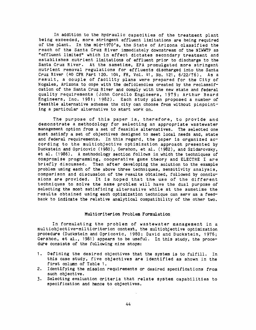
This paper is concerned with the application of multiobjective,multicriterion decision -making techniques to select an appropriatewastewater management scheme. Selection is made from a finite set offeasible alternative candidates. Furthermore, the selected scheme isexpected to satisfy a finite set of wastewater treatment projectobjectives. The specific case under consideration is the NogalesInternational Wastewater management project which treats wastewatercoming from the twin cities of Nogales, Arizona (U.S.A) and Nogales,Sonora (Mexico). Three types of decision making aids are utilized to dothe selection process so that their outcomes can be compared. Thedecision making aids are compromise programming (Zeleny, 1973, 1974),cooperative game theory (Nash, 1953; Szidarovszky, et al., 1984) andELECTRE I (Benayoun, et al., 1966).

The situation of the case study can be summarized as follows. In1951, a wastewater treatment plant of the activated sludge type wasconsturcted to provide a primary and secondary wastewater treatment with

a total capacity of 6058 m3 (1.6 mgd) for a connected population of20,000 on both sides of the border. This plant served adequately untilthe early 1960's when rapid growth of the twin cities resulted in theplant being overloaded. In 1972, a new plant, the Nogales InternationalWastewater Treatment Plant (NIWWTP) was designed and constructed some14.2 km north of the International Boundary line at the confluence ofNogales Wash and Santa Cruz River. The design treatment capacity was

31045 m3 (8.2 mgd) per day of wastewater inflow and a total populationof 102,000 (McNealy, et al., 1973). Soon this was also found to bequite inadequate. This is due to, firstly, the continuous phenomenalpopulation growth in the area. In 1985, the total population in thetwin cities was estimated to be 250,000, discharging a daily average

wastewater inflow of 33,770 m3 (8.9 mgd) directly into the treatmentplant. This is 9% above the design capacity. Secondly, accumulatedsludge deposits occupied about one -third of the available pond spacemaking the plant operate at less than 70% of its design capacity. Theresult, under existing conditions, is that the wastewater cannot betreated to the original design of satisfying minimum quality requirementlevel before it is discharged to the Santa Cruz River Channel.

43

In addition to the hydraulic capacities of the treatment plantbeing exceeded, more stringent effluent limitations are being requiredof the plant. In the mid- 1970's, the State of Arizona classified thereach of the Santa Cruz River immediately downstream of the NIWWTP as"effluent limited" which in effect dictates secondary treatment andestablishes nutrient limitations of effluent prior to discharge to theSanta Cruz River. At the sametime, EPA promulgated more stringentnutrient removal regulations for effluents discharged into the SantaCruz River (40 CFR Part 120. 104, FR, Vol. 41, No. 121, 6/22/76). As aresult, a couple of facility plans were prepared for the City ofNogales, Arizona to cope with the deficiencies created by the reclassif-cation of the Santa Cruz River and comply with the new state and federalquality requirements (John Corollo Engineers, 1979; Arthur BeardEngineers, Inc. 1981; 1982). Each study plan proposed a number offeasible alternative schemes the city can choose from without pinpoint-ing a particular alternative to start work on.

The purpose of this paper is, therefore, to provide anddemonstrate a methodology for selecting an appropriate wastewatermanagement option from a set of feasible alternatives. The selected onemust satisfy a set of objectives designed to meet local needs and, stateand federal requirements. In this regard, the paper is organized ac-cording to the multiobjective optimization approach presented byDuckstein and Opricovic (1980), Gershon, et al. (1982), and Szidarovsky,et al. (1986). A methodology section follows in which the techniques ofcompromise programming, cooperative game theory and ELECTRE I arebriefly discussed. Then after developing the solution to the exampleproblem using each of the above three techniques, sensitivity analysis,comparison and discussion of the results obtained, followed by conclu-sions are provided. It is hoped that the use of the differenttechniques to solve the same problem will have the dual purpose ofselecting the most satisficing alternative while at the sametime theresults obtained using each optimization technique can sery as a feed-back to indicate the relative analytical compatibility of the other two.

Multicriterion Problem Formulation

In formulating the problem of wastewater management in amultiobjective -milticriterion context, the multiobjective optimizationprocedure ( Duckstein and Opricovic, 1980; David and Duckstein, 1976;Gershon, et al., 1981) appears to be useful. In this study, the proce-dure consists of the following nine stops:

1. Defining the desired objectives that the system is to fulfill. Inthis case study, five objectives are identified as shown in thefirst column of Table 1.

2. Identifying the mission requirements or desired specifications fromsuch objective.

3. Selecting evaluation criteria that relate system capabilities tospecification and hence to objectives.

44

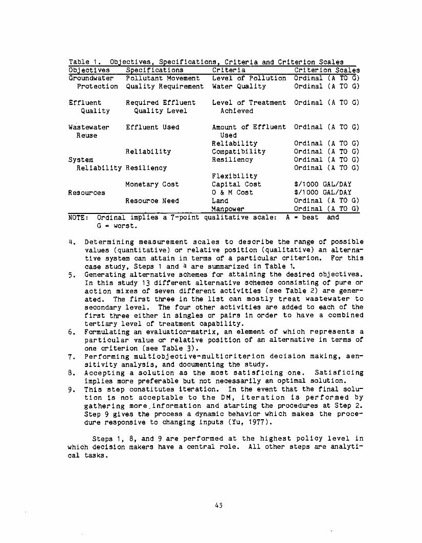
Table 1. Objectives, Specifications, Criteria and Criterion ScalesObjectives Specifications Criteria Criterion ScalesGroundwater Pollutant Movement Level of Pollution Ordinal (A TO G)

Protection Quality Requirement Water Quality Ordinal (A TO G)

EffluentQuality

WastewaterReuse

Required EffluentQuality Level

Effluent Used

ReliabilitySystemReliability Resiliency

Monetary CostResources

Resource Need

Level of Treatment Ordinal (A TO G)Achieved

Amount of Effluent Ordinal (A TO G)Used

ReliabilityCompatibilityResiliency

FlexibilityCapital Cost0 & M CostLand

Ordinal (A TO G)Ordinal (A TO G)Ordinal (A TO G)Ordinal (A TO G)

$/1000 GAL /DAY$/1000 GAL /DAY

Ordinal (A TO G)Manpower Ordinal (A TO G)

NOTE: Ordinal implies a 7-point qualitative scale: A - best and

G - worst.

4. Determining measurement scales to describe the range of possiblevalues (quantitative) or relative position (qualitative) an alterna-tive system can attain in terms of a particular criterion. For thiscase study, Steps 1 and 4 are summarized in Table 1.

5. Generating alternative schemes for attaining the desired objectives.In this study 13 different alternative schemes consisting of pure oraction mixes of seven different activities (see Table 2) are gener-ated. The first three in the list can mostly treat wastewater tosecondary level. The four other activities are added to each of thefirst three either in singles or pairs in order to have a combinedtertiary level of treatment capability.

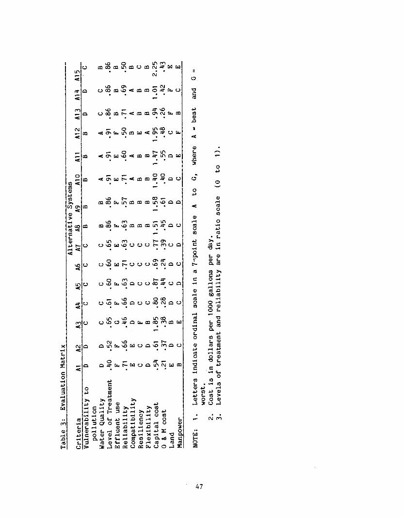
6. Formulating an evaluation-matrix, an element of which represents aparticular value or relative position of an alternative in terms ofone criterion (see Table 3).

7. Performing multiobjective- multicriterion decision making, sen-sitivity analysis, and documenting the study.

8. Accepting a solution as the most satisficing one. Satisficingimplies more preferable but not necessarily an optimal solution.

9. This step constitutes iteration. In the event that the final solu-tion is not acceptable to the DM, iteration is performed bygathering more ,information and starting the procedures at Step 2.Step 9 gives the process a dynamic behavior which makes the proce-dure responsive to changing inputs (Yu, 1977).

Steps 1, 8, and 9 are performed at the highest policy level inwhich decision makers have a central role. All other steps are analyti-cal tasks.

45

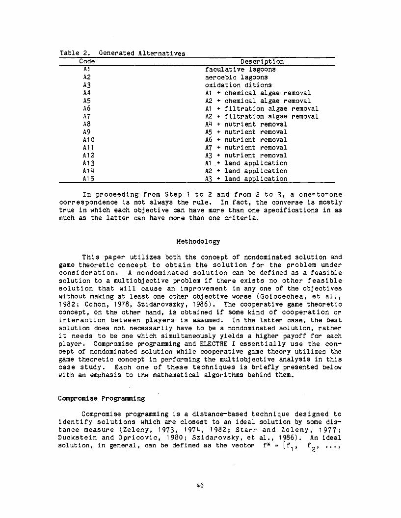
Table 2. Generated AlternativesCodeAl

A2A3

A4A5

A6

A7A8

A9

A10All

Al2Al 3

A14A15

Descriptionfaculative lagoonsaeroebic lagoonsoxidation ditionsAl + chemical algae removalA2 + chemical algae removalAl + filtration algae removalA2 + filtration algae removalA4 + nutrient removalAS + nutrient removalA6 + nutrient removalA7 + nutrient removalA3 + nutrient removalA1_+ land applicationA2 + land applicationA3 + land application

In proceedicorrespondence istrue in which eachmuch as the latter

ng from Step 1 to 2 and from 2 to 3, a one-to -onenot always the rule. In fact, the converse is mostlyobjective can have more than one specifications in ascan have more than one criteria.

Methodology

This paper utilizes both the concept of nondominated solution andgame theoretic concept to obtain the solution for the problem underconsideration. A nondominated solution can be defined as a feasiblesolution to a multiobjective problem if there exists no other feasiblesolution that will cause an improvement in any one of the objectiveswithout making at least one other objective worse (Goicoechea, et al.,1982; Cohon, 1978, Szidarovszky, 1986). The cooperative game theoreticconcept, on the other hand, is obtained if some kind of cooperation orinteraction between players is assumed. In the latter case, the bestsolution does not necessarily have to be a nondominated solution, ratherit needs to be one which simultaneously yields a higher payoff for eachplayer. Compromise programming and ELECTRE I essentially use the con-cept of nondominated solution while cooperative game theory utilizes thegame theoretic concept in performing the multiobjective analysis in thiscase study. Each one of these techniques is briefly presented belowwith an emphasis to the mathematical algorithms behind them.

Compromise Programming

Compromise programming is a distance -based technique designed toidentify solutions which are closest to an ideal solution by some dis-tance measure (Zeleny, 1973, 1974, 1982; Starr and Zeleny, 1977;Duckstein and Opricovic, 1980; Szidarovsky, et al., 1986). An idealsolution, in general, can be defined as the vector f* _ (f1, f2, ...,

46

tt1UCO CO ti3 üd1CO 00 N W W

.- CV

1/4O CT .- NC] UCOCS1/4OctCC3md.Z" Cs,U

.

vo.-p 000CiItiaCnCtaONNCsmaNa CO

d tn CO:C CT Cs, tt1 rra W a U Es.

leEM

C0 dONWaCOm?1.f1p Wa

a

a

-- -- O OC17 tCTW C-4tCnCL!??pU

CO CO Cr tf m CO t13 tt1 G p pCO

W MI - thW m CO Cs. t0 CO CO CO tf1.=" p U

.

t!1 01 t- CTU U4O W W U O U t-MO p

UO - O«

U40 Cs3P-UO NpU

n

C5

ro

Oa)p

a)

L

O

UO

o

ca ol:r y.)OOU C.a Cs.íppCJUCpU p .-i-1

. 1 .1C) ro .O.-I CO ro- k.O 0 CO c0 Vw

U UvOCs.qOpUOCONpU pC),)

O L'-i r

U UvDC7pCr.CACOMC7S W C L L. .., a3 ro= 'CI 0.

L .+-)

O CO

Lç,,,

C

p Co Ú1 Cs. W U C3 O M p U a) c0 Ey> ...I JJro -I CO

. .

O O C- O

p pts.t-- WUp in NW CII tC ,~,.e 4.4 4.4

.4-) 0") mO

o aC) o , .4.4 CO

.0 E 4.) co 4.) C)

> >,m >> a)óó', w.,.) 4.)0)0 i.) 4.) a3Ua-+ C -+ L. CO A -+ >I V)ri O.-iH O >si.) O++r ...4 .I ...r C,) .r O cl)13 y.) g 4-4 yl .-1 A i',. .-i O L r N enLCO-..-=i O O Ñ Á ..Oc cu O 3CD ,-4 L.-1 O ro ro c .-c 4.3 Sc OO O O a) -+ .r C3. >a -.-4 T) - W

0. Ñ a) w E.ai cCtf tO0 Ó

> 3..3 W C>rUC1C Cc. 00..5= z

47

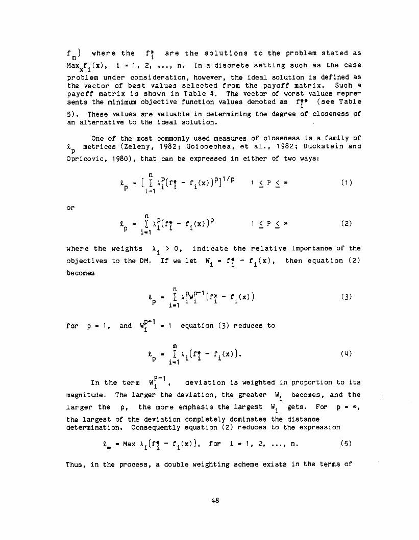
fn) where the fi are the solutions to the problem stated as

Maxxfi(x), i = 1, 2, ..., n. In a discrete setting such as the case

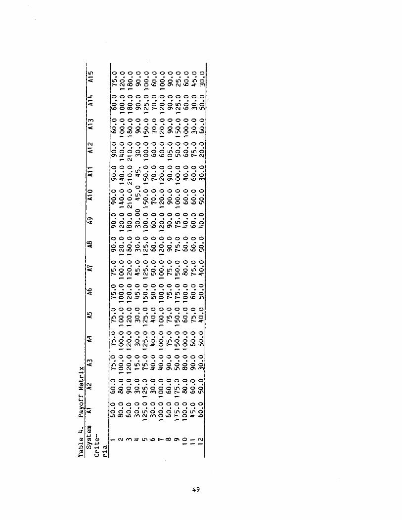
problem under consideration, however, the ideal solution is defined asthe vector of best values selected from the payoff matrix. Such apayoff matrix is shown in Table 4. The vector of worst values repre-sents the minimum objective function values denoted as fi* (see Table

5). These values are valuable in determining the degree of closeness ofan alternative to the ideal solution.

One of the most commonly used measures of closeness is a family ofßp metrices (Zeleny, 1982; Goicoechea, et al., 1982; Duckstein and

Opricovic, 1980), that can be expressed in either of two ways:

or

n

Qp [ E ap(fi - fi(x))P 1/ P

ii=1

n

EaP(fi - fl(x))P

i=1

1 < P < (1)

1 <P <co (2)

where the weights X > 0, indicate the relative importance of the

objectives to the DM. If we let Wi = fi - fi(x), then equation (2)

becomes

n

t = L apW. 1(fl fi(x))i=1

for p = 1, and Wp -1 = 1 equation (3) reduces to

m

ßp = ai(fi - fi(x)).1=1

(3)

(4)

In the term WP -1er , deviation is weighted in proportion to its

magnitude. The larger the deviation, the greater Wi becomes, and the

larger the p, the more emphasis the largest Wi gets. For p = ,the largest of the deviation completely dominates the distancedetermination. Consequently equation (2) reduces to the expression

= Max ai(f* - fi(x)), for i 1, 2, ..., n.i

(5)

Thus, in the process, a double weighting scheme exists in the terms of

48

O O O O O O O O O O O OU1000000011100 0N N 00 Ch O 4) O CA N 4O ? M

r- r r- r-

O O O O O O O O O O O OO O O o 0 0 0 0 L11 0 0 04D O 00 Ch N N N Ch N 40 M LC1r- r- r

m O O O O O O O O O O O OO O O O O O O O O O O O4O 000 CA UINCV CMU10 014D

.- r- r- '- r-

N

O

CO

MQ

(V

4

CD O O O O O O O O O O OO OOOOOOUIOO OC\ ? r- M O4O VO O Ú14O N- N

r- CU r- r-

O O O 0 0 0 0 0 0 0 0U10 0 0 0 0 0 0 0 0 0 01(1NN CmOO M

r- tV r- r- r-0

O O O 0 0 0 0 0 0 0 00 0 0=r 0 0 0 0 0 0 0 0Cm .? r- LC1 N- N Cm O mD 4) U1

r- N 0O O O O O O O O O O O OO O O O O O O O L 11 0 0 0CAN00 01 O4O N CmN-?4D?

0 0 0 0 0 0 0 0 0 0 0 0O 00000000000

CV c0 MN N CMN-4)4D U1

0 0 0 0 0 0 0 0 0 0 0 0L11 0 O Ú1 U1 0 O Ú1 0 O U1 ON O N Zr N 111 O N- L11 00 N- .7

O O O O O O O O O O O OU1 00111000L11U1000N- O N? U1 Ul O N- CD 40 Ul

O O O O O O O O O O O OU1000t1100Ú100U10N ON MN?ON-U1%.ON?

r- r- r r-O 0 0 0 0 0 0 0 0 0 0 0L11 0 001f100 U10000N O N 01N.7 O NU104D U1

r- r r rCD O O O O O O O O O O OU100 tC1U10000000N 0 (V r N?? 01U100ChM

O O O O O O O O O O O OO OOOÚ1000LC10004) 00 Om 01 cm 01 04O N 00 4) U1

O 0 0 0 0 0 0 0 0 0 0 0O 000111000L110U104) 00 4D M N 01 0 4O N O=r 4)r- r- r-

r- C4014. LC1 O N 00 ON O r- Nr-r-r-

49

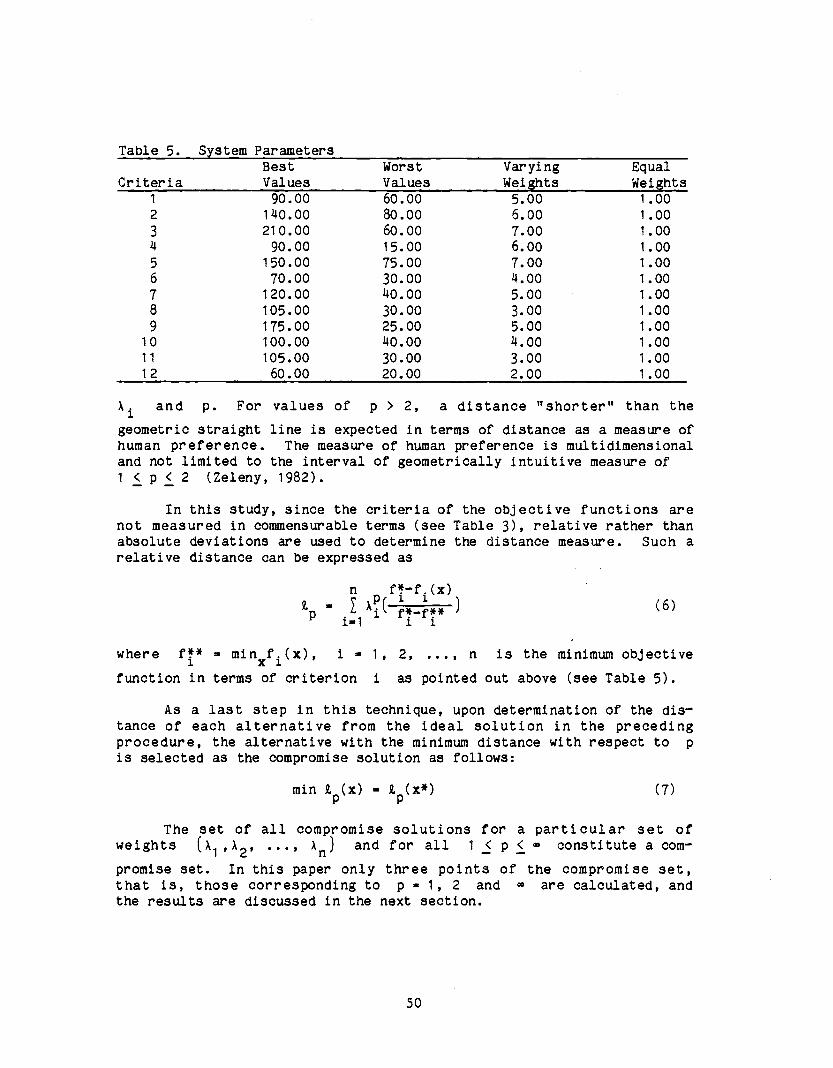
Table 5. System Parameters

CriteriaBestValues

WorstValues

VaryingWeights

EqualWeights

1 90.00 60.00 5.00 1.002 140.00 80.00 6.00 1.003 210.00 60.00 7.00 1.004 90.00 15.00 6.00 1.00

5 150.00 75.00 7.00 1.006 70.00 30.00 4.00 1.00

7 120.00 40.00 5.00 1.008 105.00 30.00 3.00 1.00

9 175.00 25.00 5.00 1.0010 100.00 40.00 4.00 1.0011 105.00 30.00 3.00 1.0012 60.00 20.00 2.00 1.00

Ai and p. For values of p > 2, a distance "shorter" than the

geometric straight line is expected in terms of distance as a measure ofhuman preference. The measure of human preference is multidimensionaland not limited to the interval of geometrically intuitive measure of1 < p < 2 (Zeleny, 1982).

In this study, since the criteria of the objective functions arenot measured in commensurable terms (see Table 3), relative rather thanabsolute deviations are used to determine the distance measure. Such arelative distance can be expressed as

n fi-fi(x)

_Qp

ii

=1 i i(6)

where fi* = minxfi(x), i = 1, 2, ..., n is the minimum objective

function in terms of criterion i as pointed out above (see Table 5).

As a last step in this technique, upon determination of the dis-tance of each alternative from the ideal solution in the precedingprocedure, the alternative with the minimum distance with respect to p

is selected as the compromise solution as follows:

min t(x) = t(x *) (7)

The set of all compromise solutions for a particular set ofweights (À1,X2, ..., an) and for all 1 < p < = constitute a com-

promise set. In this paper only three points of the compromise set,that is, those corresponding to p = 1, 2 and = are calculated, andthe results are discussed in the next section.

50

ELECTRE I

ELECTRE I which stands for elimination and (et) choice translatingalgorithm, was initially developed by Benayoun, Roy and Sussman (1966)and improved by Roy (1971). A fundamental feature of ELECTRE I is theuse of pairwise comparisons among members of a set of alternative sys-tems in order to eliminate a subset of less desirable alternatives whilechoosing those systems which are preferred for most of the criteriawithout causing an unacceptable level of discontent for any onecriterion (Nijkamp and Delft, 1977; Gershon, et al., 1982). Therefore,both elimination and choice are essential ingredients of ELECTRE I. The

methodology involves three important concepts: concordance, discordance,and threshold values.

The concordance between any two alternative actions m and n is

a weighted measure of the number of criteria for which action m is

weakly preferred to action n (mPn or mEn, that is, action m is

more preferred or equally preferred to action n). Now, if we let Xi,

i = 1, 2, ..., N represent the weight given a priori to criterion i

by the decision maker for use in a specific algorithm, then the concor-dance (or concord) index between actions m and n can be determinedas follows:

N

C(m,n) _ / ai/( E ai)iES(m,n) i=1

(8)

where S(m,n) _ (ilmPn mEn }, that is, the set of all criteria forwhich m is preferred to n or equal to n. The weights, Xi. which

are elicited form the decision maker, reflect his/her preferencestructure. The concordance matrix, C(m,n) can be thought of as repre-senting the weighted percentage of all criteria for which one action isweakly preferred to another. By definition, 0 < C(m,n) < 1.

Discordance is complementary to the concordance concept.Accordingly, discordance represents the discomfort one experiences whenconfronted with the less preferred member of two possible pairs. Tocompute the discordance matrix in this study, each criterion is assigneda different range of scales, the upper value of which ranging from 70

to 210 (see Tables 5 and 6). In other cases, an interval scale commonto each criterion is usually defined. In any case, the interval scaleis subjectively determined to represent the degree of dissatisfactionthe DM may experience in moving from one point scale to the next lessdesirable point scale in one criterion compared with similar trend inanother criterion. A seven -point scale is selected for each criterionin order to enable the widest possible levels of discomfort the DM canassign in moving from the best to the worst levels of each criterion(Gershon, et al., 1982). With this understanding, the discordanceindex, D(m,n), can be defined as

51

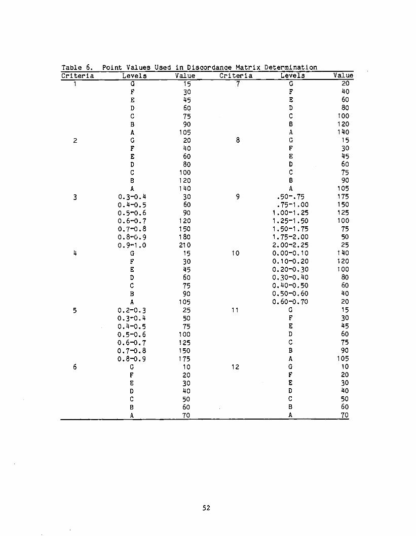
Table 6. Point Values Used in Discordance Matrix DeterminationCriteria Levels Value Criteria Levels Value

1 G 15 7 G 20

F 30 F 40

E 45 E 60

D 60 D 80

C 75 C 100

B 90 B 120

A 105 A 140

2 G 20 8 G 15

F 40 F 30

E 60 E 45

D 80 D 60

C 100 C 75

B 120 B 90

A 140 A 105

3 0.3-0.4 30 9 .50-.75 175

0.4-0.5 60 .75-1.00 150

0.5-0.6 90 1.00-1.25 125

0.6-0.7 120 1.25-1.50 100

0.7-0.8 150 1.50-1.75 75

0.8-0.9 180 1.75-2.00 50

0.9-1.0 210 2.00°2.25 25

4 G 15 10 0.00-0.10 140

F 30 0.10-0.20 120

E 45 0.20-0.30 100

D 60 0.30-0.40 80

C 75 0.40-0.50 60

B 90 0.50-0.60 40

A 105 0.60-0.70 20

5 0.2-0.3 25 11 G 15

0.3-0.4 50 F 30

0.4-0.5 75 E 450.5-0.6 100 D 60

0.6-0.7 125 C 75

0.7-0.8 150 B 90

0.8-0.9 175 A 105

6 G 10 12 G 10

F 20 F 20

E 30 E 30

D 40 D 40

C 50 C 50

B 60 B 60

A 70 A 70

52

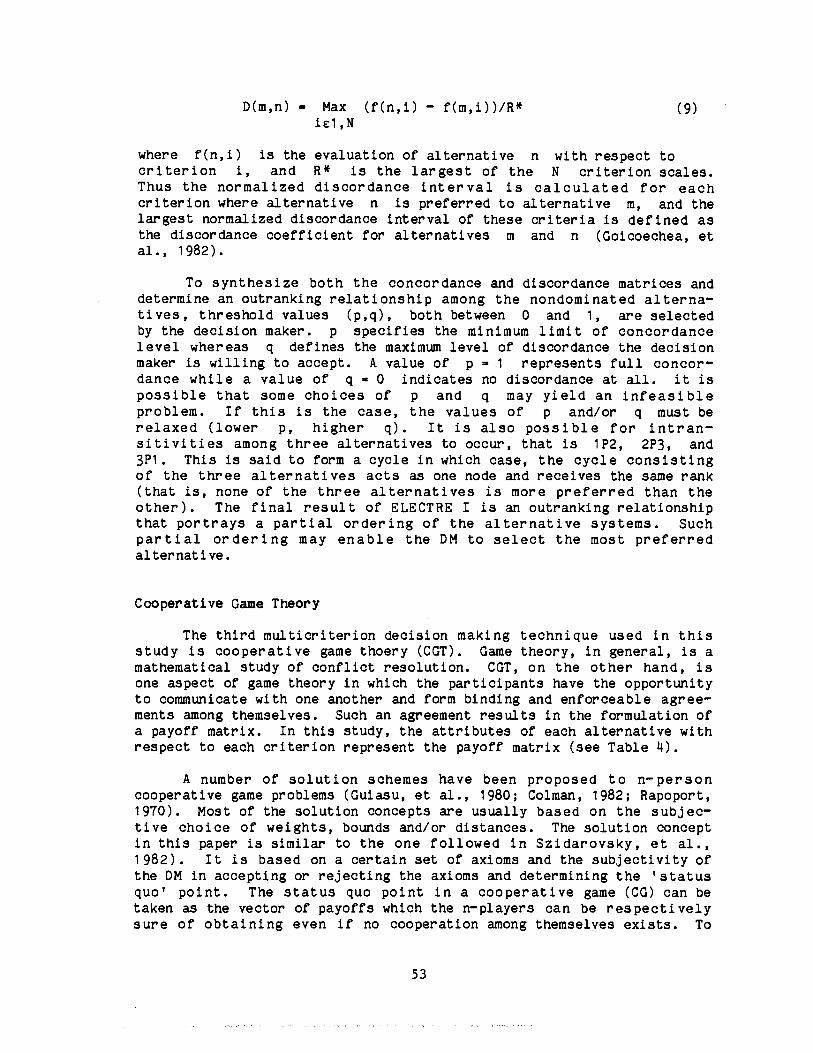
D(m,n) = Max (f(n,i) - f(m,i)) /R* (9)

ie1,N

where f(n,i) is the evaluation of alternative n with respect tocriterion i, and R* is the largest of the N criterion scales.Thus the normalized discordance interval is calculated for eachcriterion where alternative n is preferred to alternative m, and thelargest normalized discordance interval of these criteria is defined asthe discordance coefficient for alternatives m and n (Goicoechea, etal., 1982).

To synthesize both the concordance and discordance matrices anddetermine an outranking relationship among the nondominated alterna-tives, threshold values (p,q), both between 0 and 1, are selectedby the decision maker. p specifies the minimum limit of concordancelevel whereas q defines the maximum level of discordance the decisionmaker is willing to accept. A value of p = 1 represents full concor-dance while a value of q = 0 indicates no discordance at all. it ispossible that some choices of p and q may yield an infeasibleproblem. If this is the case, the values of p and /or q must berelaxed (lower p, higher q). It is also possible for intran-sitivities among three alternatives to occur, that is 1P2, 2P3, and3P1. This is said to form a cycle in which case, the cycle consistingof the three alternatives acts as one node and receives the same rank(that is, none of the three alternatives is more preferred than theother). The final result of ELECTRE I is an outranking relationshipthat portrays a partial ordering of the alternative systems. Suchpartial ordering may enable the DM to select the most preferredalternative.

Cooperative Game Theory

The third multicriterion decision making technique used in thisstudy is cooperative game thoery (CGT). Game theory, in general, is amathematical study of conflict resolution. CGT, on the other hand, isone aspect of game theory in which the participants have the opportunityto communicate with one another and form binding and enforceable agree-ments among themselves. Such an agreement results in the formulation ofa payoff matrix. In this study, the attributes of each alternative withrespect to each criterion represent the payoff matrix (see Table 4).

A number of solution schemes have been proposed to n-personcooperative game problems (Guiasu, et al., 1980; Colman, 1982; Rapoport,1970) . Most of the solution concepts are usually based on the subjec-tive choice of weights, bounds and /or distances. The solution conceptin this paper is similar to the one followed in Szidarovsky, et al.,1982). It is based on a certain set of axioms and the subjectivity ofthe DM in accepting or rejecting the axioms and determining the 'statusquo' point. The status quo point in a cooperative game (CG) can betaken as the vector of payoffs which the n- players can be respectivelysure of obtaining even if no cooperation among themselves exists. To

53

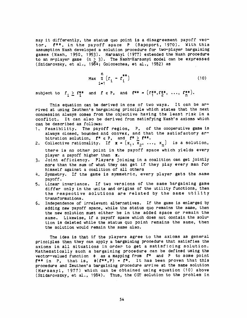
say it differently, the status quo point is a disagreement payoff vec-tor, f * *, in the payoff space P (Rapoport, 1970). With thisassumption Nash developed a solution procedure for two -player bargaininggames (Nash, 1950, 1953). Harsanyi (1977) extended the Nash procedureto an n- player game (n > 3). The Nash- Harsanyi model can be expressed(Szidarovsky, et al., 1984; Goicoechea, et al., 1982) as

n

Max R (fi - fi *)i =1

subject to fi > fi* and f s P, and f ** _ (f1 *,f2 *, f* *).n

(10)

This equation can be derived in one of two ways. It can be ar-rived at using Zeuthen's bargaining principle which states that the nextconcession always comes from the objective having the least risk in aconflict. It can also be derived from satisfying Nash's axioms whichcan be described as follows:1. Feasibility. The payoff region, P, of the cooperative game is

always closed, bounded and convex, and that the satisfactory ar-bitration solution, f* a P, and f* > f * *.

2. Collective rationality. If x = (x1, 7 ..., xn) is a solution,

there is no other point in the payoff space which yields everyplayer a payoff higher than x.

3. Joint efficiency. Players joining in a coalition can get jointlymore than the sum of what they can get if they play every man forhimself against a coalition of all others

4. Symmetry. If the game is symmetric, every player gets the samepayoff.

5. Linear invariance. If two versions of the same bargaining gamediffer only in the units and origins of the utility functions, thenthe respective solutions are related by the same utilitytransformations.

6. Independence of irrelevant alternatives. If the game is enlarged byadding new payoff space, while the status quo remains the same, thenthe new solution must either be in the added space or remain thesame. Likewise, if a payoff space which does not contain the solu-tion is deleted while the status quo point remains the same, thenthe solution would remain the same also.

The idea is that if the players agree to the axioms as generalprinciples then they can apply a bargaining procedure that satisfies theaxioms in all situations in order to get a satisficing solution.Mathematically such a bargaining procedure can be defined using thevector -valued function 4 as a mapping from f* and P to some pointf ** in P, that is, 4(f * *,P) = f *. It has been proven that thisprocedure and Zeuthen's bargaining procedure arrive at the same solution(Harsanyi, 1977) which can be obtained using equation (10) above(Szidarovszky, et al., 1984). Thus, the CGT solution to the problem in

54

this paper is obtained using equation (10), and the results are dis-cussed in the next section along with the solutions obtained usingcompromise programming and ELECTRE I.

Application and Analysis

In this section of the paper, analysis of application of com-promise programming, ELECTRE I, and cooperative game theory to theNogales (Arizona -Sonora) international wastewater management problem arediscussed. After the evaluation matrix (Table 3) for the case problemhas been obtained using the multiobjective optimization procedure, allthe array elements in the matrix are quantified (Table 4) to make theproblem suitable for analysis using the three techniques. This quan-tification is based upon the range of scales selected for each criterionby the DM. In this study the DM's preferences are an approximatedaverage of the documented needs and desires of the parties involved(Arthur Beard Engineers, Inc., 1982, 1981, John Carollo, Engineers,1979). These parties include the local community, the State of Arizona,the U. S. EPA, and the International Boundary and Water Commission(U.S.- Mexico).

Three separate computer algorithms, one for each technique, havebee used to analyze the problem. The quantified payoff matrix (Table 4)has been used as a homogeneous input into the programs.

Compromise Programming

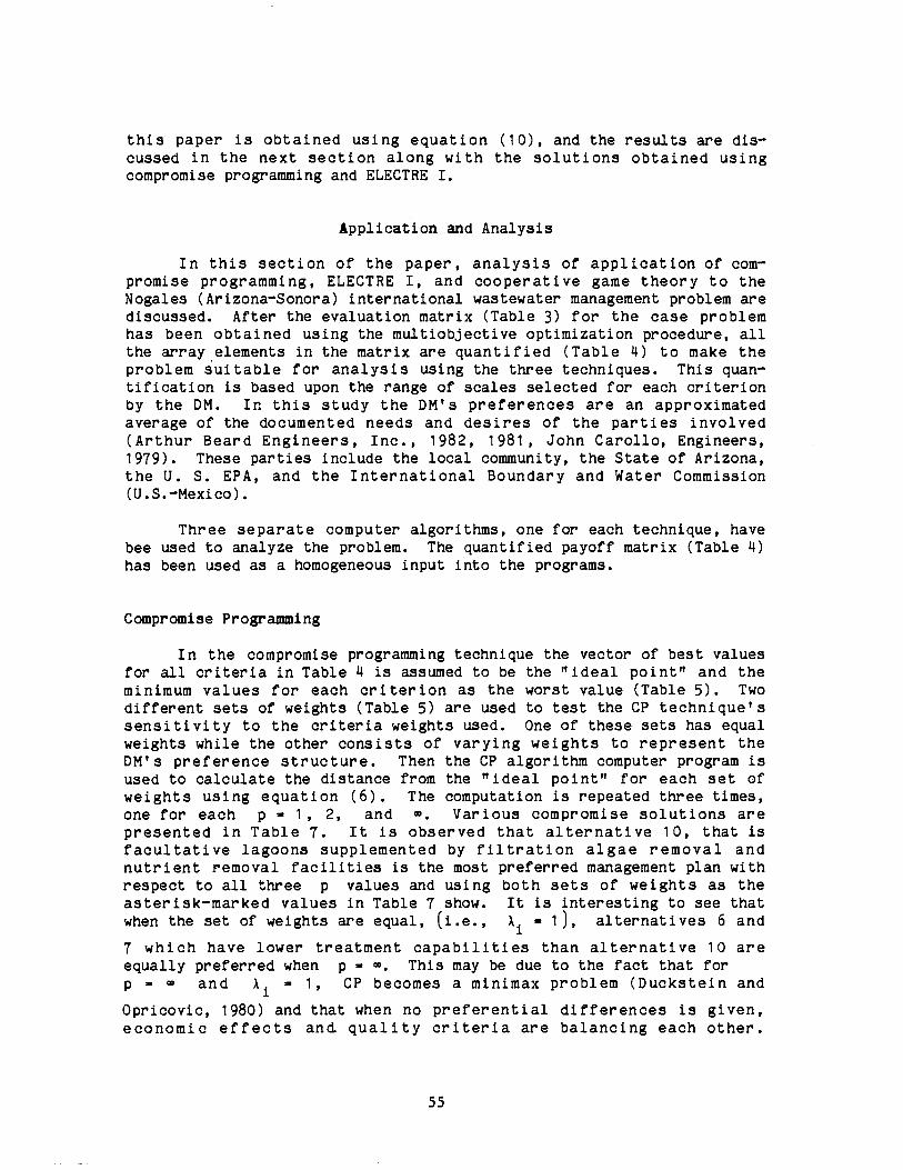
In the compromise programming technique the vector of best valuesfor all criteria in Table 4 is assumed to be the "ideal point" and theminimum values for each criterion as the worst value (Table 5). Twodifferent sets of weights (Table 5) are used to test the CP technique'ssensitivity to the criteria weights used. One of these sets has equalweights while the other consists of varying weights to represent theDM's preference structure. Then the CP algorithm computer program isused to calculate the distance from the "ideal point" for each set ofweights using equation (6). The computation is repeated three times,one for each p = 1, 2, and ce. Various compromise solutions arepresented in Table 7. It is observed that alternative 10, that isfacultative lagoons supplemented by filtration algae removal andnutrient removal facilities is the most preferred management plan withrespect to all three p values and using both sets of weights as theasterisk -marked values in Table 7 show. It is interesting to see thatwhen the set of weights are equal, (i.e., Xi = 1), alternatives 6 and

7 which have lower treatment capabilities than alternative 10 areequally preferred when p = m. This may be due to the fact that forp = and Xi = 1, CP becomes a minimax problem (Duckstein and

Opricovic, 1980) and that when no preferential differences is given,economic effects and quality criteria are balancing each other.

55

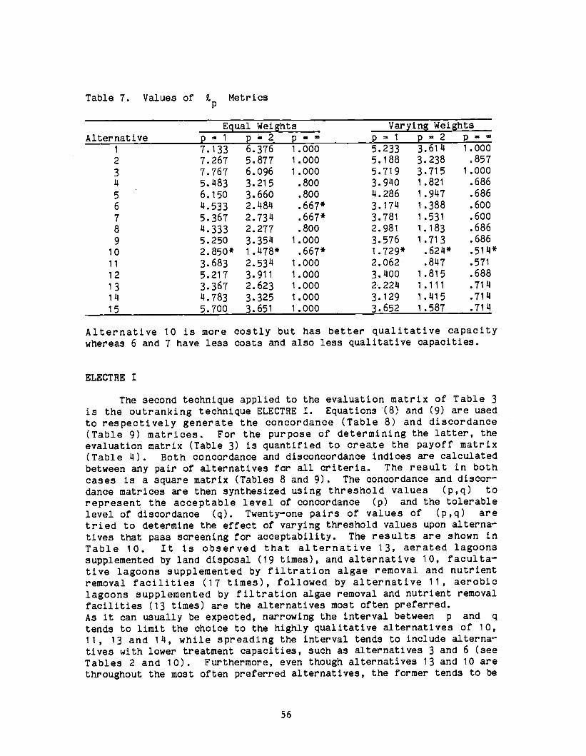
Table 7. Values of k Metrics

AlternativeEqual Weights Varying Weights

p= 1 p- 2 p= p= 1 p= 2 p= m1 7.133 6.376 1.000 5.233 3.614 1.000

2 7.267 5.877 1.000 5.188 3.238 .857

3 7.767 6.096 1.000 5.719 3.715 1.000

4 5.483 3.215 .800 3.940 1.821 .686

5 6.150 3.660 .800 4.286 1.947 .686

6 4.533 2.484 .667* 3.174 1.388 .600

7 5.367 2.734 .667* 3.781 1.531 .600

8 4.333 2.277 .800 2.981 1.183 .686

9 5.250 3.354 1.000 3.576 1.713 .686

10 2.850* 1.478* .667* 1.729* .624* .514*

11 3.683 2.534 1.000 2.062 .847 .571

12 5.217 3.911 1.000 3.400 1.815 .688

13 3.367 2.623 1.000 2.224 1.111 .714

14 4.783 3.325 1.000 3.129 1.415 .714

15 5.700 3.651 1.000 3.652 1.587 .714

Alternative 10 is more costly but has better qualitative capacitywhereas 6 and 7 have less costs and also less qualitative capacities.

ELECTRE I

The second technique applied to the evaluation matrix of Table 3is the outranking technique ELECTRE I. Equations (8) and (9) are usedto respectively generate the concordance (Table 8) and discordance(Table 9) matrices. For the purpose of determining the latter, theevaluation matrix (Table 3) is quantified to create the payoff matrix(Table 4). Both concordance and disconcordance indices are calculatedbetween any pair of alternatives for all criteria. The result in bothcases is a square matrix (Tables 8 and 9). The concordance and discor-dance matrices are then synthesized using threshold values (p,q) to

represent the acceptable level of concordance (p) and the tolerable

level of discordance (q). Twenty-one pairs of values of (p,q) aretried to determine the effect of varying threshold values upon alterna-tives that pass screening for acceptability. The results are shown inTable 10. It is observed that alternative 13, aerated lagoonssupplemented by land disposal (19 times), and alternative 10, faculta-tive lagoons supplemented by filtration algae removal and nutrientremoval facilities (17 times), followed by alternative 11, aerobiclagoons supplemented by filtration algae removal and nutrient removalfacilities (13 times) are the alternatives most often preferred.As it can usually be expected, narrowing the interval between p and q

tends to limit the choice to the highly qualitative alternatives of 10,11, 13 and 14, while spreading the interval tends to include alterna-tives with lower treatment capacities, such as alternatives 3 and 6 (see

Tables 2 and 10). Furthermore, even though alternatives 13 and 10 arethroughout the most often preferred alternatives, the former tends to be

56

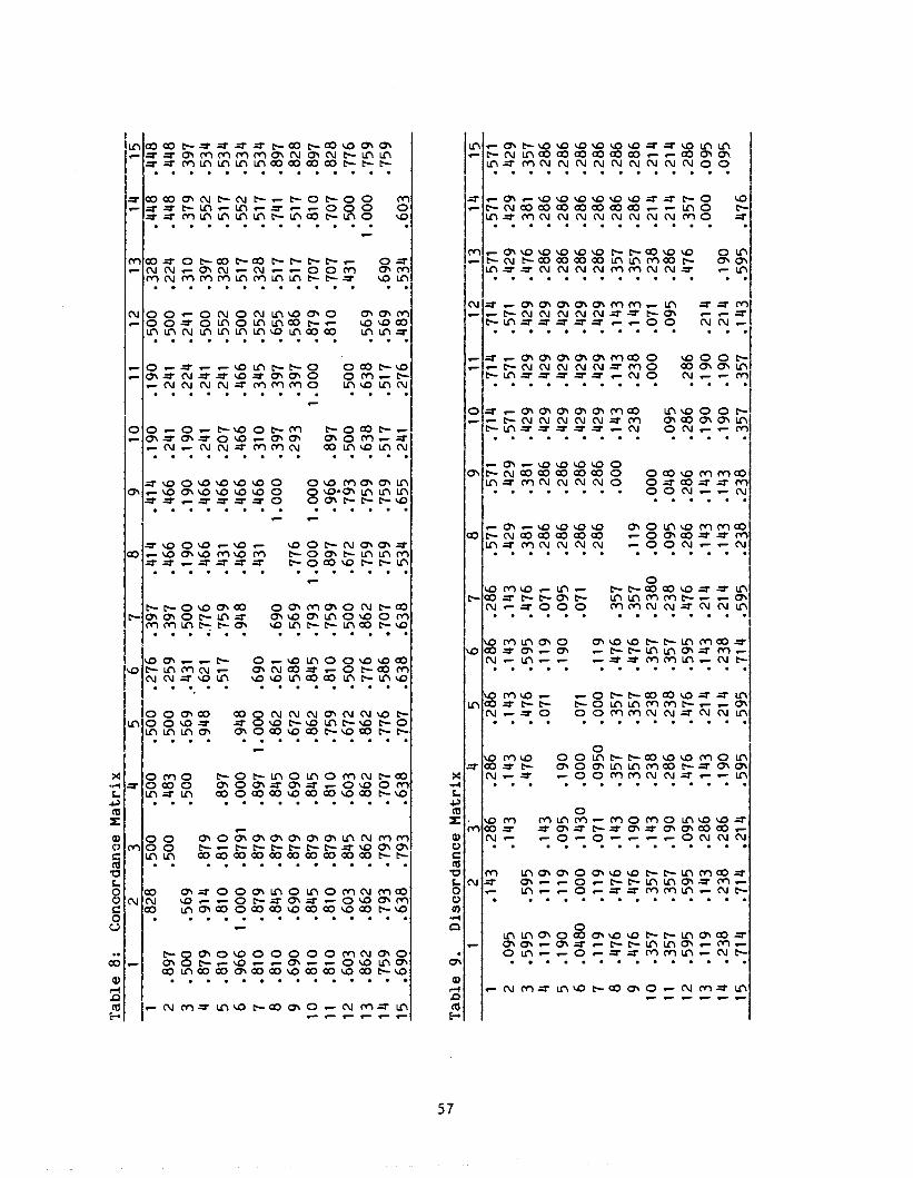
Table 8:

Concordance Matrix

12

34

56

78

910

11

12

13

14

15

.828

.500

.500

.500

.276

.397

.414

.414

.190

.190

.500

.328

.448

.448

2.897

.500

.483

.500

.259

.397

.466

.466

.241

.241

.500

.224

.448

.448

3.500

.569

.500

.569

,.431

.500

.190

.190

.190

.224

.241

.310

.379

.397

4.879

.914

.879

.948

.621

..776

.466

.466

.241

.241

.500

.397

.552

.534

5.810

.810

.810

.897

.517

.759

.431

.466

.207

.241

.552

.328

.517

.534

6.966

1.000

.8791

.000

.948

.948

.466

.466

.466

.466

.500

.517

.552

.534

7.810

.879

.879

.897

1.000

.690

.431

.466

.310

.345

.552

.328

.517

.534

8.810

.845

.879

.845

.862

.621

.690

1.000

.397

.397

.655

.517

.741

.897

9.690

.690

.879

.690

.672

.586

.569

.776

.293

.397

.586

.517

.517

.828

10

.810

.845

.879

.845

.862

.845

.793

1.000

1.000

1.000

.879

.707

.810

.897

11

.810

.810

.879

.810

.759

.810

.759

.897

.966

.897

.810

.707

.707

.828

12

.603

.603

.845

.603

.672

.500

.500

.672

.793

.500

.500

.431

.500

.776

13

.862

.862

.862

.862

.862

.776

.862

.759

.759

.638

.638

.569

1.000

.759

14

.759

.793

.793

.707

.776

.586

.707

.759

.759

.517

.517

.569

.690

.759

15

.690

.638

.793

.638

.707

.638

.638

.534

.655

.241

.276

.483

.534

.603

Table 9.

Discordance Matrix

12

34

56

78

910

11

12

13

14

15

1.143

.286

.286

.286

.286

.286

.571

.571

.714

.714

.714

.571

.571

.571

2.095

.143

.143

.143

.143

.143

.429

.429

.571

.571

.571

.429

.429

.429

3.595

.595

.476

.476

.595

.476

.381

.381

.429

.429

.429

.476

.381

.357

4.119

.119

.143

.071

.119

.071

.286

.286

.429

.429

.429

.286

.286

.286

5.190

.119

.095

.190

.190

.095

.286

.286

.429

.429

.429

.286

.286

.286

6.0480

.000

.1430

.000

.071

.071

.286

.286

.429

.429

.429

.286

.286

.286

7.119

.119

.071

.0950

.000

.119

.286

.286

.429

.429

.429

.286

.286

.286

8.476

.476

.143

.357

.357

.476

.357

.000

.143

.143

.143

357

.286

.286

9.476

.476

.190

.357

.357

.476

.357

.119

.238

.238

.143

.357

.286

.286

10

.357

.357

.143

.238

.238

.357

.2380

.000

.000

.000

.071

.238

.214

.214

11

.357

.357

.190

.286

.238

.357

.238

.095

.048

.095

.095

.286

.214

.214

12

.595

.595

.095

.476

.476

.595

.476

.286

.286

.286

.286

.476

.357

.286

13

.119

.143

.286

.143

.214

.143

.214

.143

.143

.190

.190

.214

.000

.095

14

.238

.238

.286

.190

.214

.238

.214

.143

.143

.190

.190

.214

.190

.095

15

.714

.714

.214

.595

.595

.714

.595

.238

.238

.357

.357

.143

.595

.476

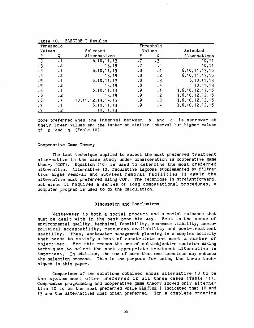
Table 10. ELECTRE I ResultsThresholdValuesP Q

SelectedAlternatives

ThresholdValues

P Q

SelectedAlternatives

.3 .1 6,10,11,13 .7 .3 10,11

.3 .2 13,15 .7 .4 10,11

.4 .1 6,10,11,13 .8 .1 6,10,11,13,15

.4 .2 13,14 .8 .2 6,10,11,13,15

.5 .1 6,10,11,13 .8 .3 6,10,11,13

.5 .2 13,14 .8 .4 10,11,13

.6 .1 6,10,11,13 .9 .1 3,6,10,12,13,15

.6 .2 13,14 .9 .2 3,6,10,12,13,15

.6 .3 10,11,12,13,14,15 .9 .3 3,6,10,12,13,15

.7 .1 6,10,11,13 .9 .4 3,6,10,12,13,15

.7 .2 10,11,13

more preferred when the interval between p and q is narrower attheir lower values and the latter at similar interval but higher valuesof p and q (Table 10).

Cooperative Game Theory

The last technique applied to select the most preferred treatmentalternative in the case study under consideration is cooperative gametheory (CGT). Equation (10) is used to determine the most preferredalternative. Alternative 10, faculative lagoons supplemented by filtra-tion algae removal and nutrient removal facilities is again thealternative most preferred using CGT. The technique is straightforward,but since it requires a series of long computational procedures, acomputer program is used to do the calculation.

Discussion and Conclusions

Wastewater is both a social product and a social nuisance thatmust be dealt with in the best possible way. Best in the sense ofenvironmental quality, technical feasibility, economic viability, socio-political acceptability, resources availability and post-treatmentusability. Thus, wastewater management planning is a complex activitythat needs to satisfy a host of constraints and meet a number ofobjectives. For this reason the use of multiobjective decision makingtechniques,to select the most appropriate treatment alternative isimportant. In addition, the use of more than one technique may enhancethe selection process. This is the purpose for using the three tech-niques in this paper.

Comparison of the solutions obtained shows alternative 10 to bethe system most often preferred in all three cases (Table 11).Compromise programming and cooperative game theory showed only alterna-tive 10 to be the most preferred while ELECTRE I indicated that 10 and13 are the alternatives most often preferred. For a complete ordering

58

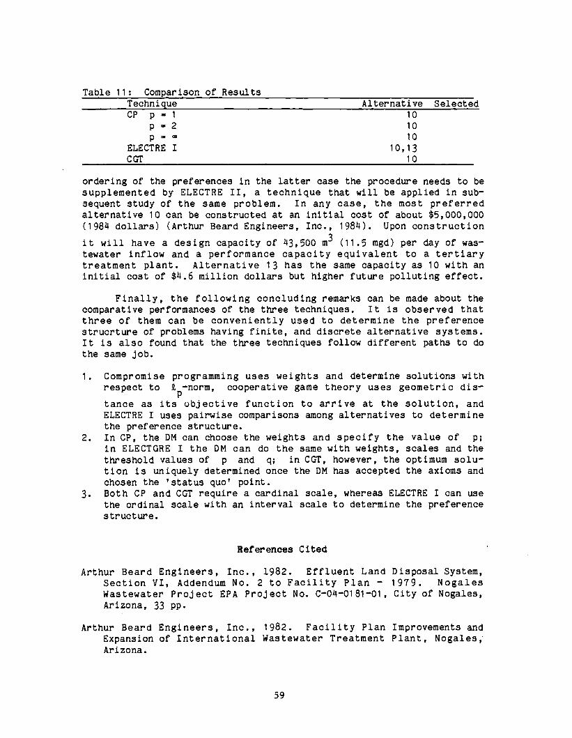
Table 11: Comparison of ResultsTechniqueCP p = 1

Alternative Selected10

p=2 10

p 10

ELECTRE I 10,13CGT 10

ordering of the preferences in the latter case the procedure needs to besupplemented by ELECTRE II, a technique that will be applied in sub-sequent study of the same problem. In any case, the most preferredalternative 10 can be constructed at an initial cost of about $5,000,000(1984 dollars) (Arthur Beard Engineers, Inc., 1984). Upon construction

it will have a design capacity of 43,500 m3 (11.5 mgd) per day of was-tewater inflow and a performance capacity equivalent to a tertiarytreatment plant. Alternative 13 has the same capacity as 10 with aninitial cost of $4.6 million dollars but higher future polluting effect.

Finally, the following concluding remarks can be made about thecomparative performances of the three techniques. It is observed thatthree of them can be conveniently used to determine the preferencestrucrture of problems having finite, and discrete alternative systems.It is also found that the three techniques follow different paths to dothe same job.

1. Compromise programming uses weights and determine solutions withrespect to Qp -norm, cooperative game theory uses geometric dis-

tance as its objective function to arrive at the solution, andELECTRE I uses pairwise comparisons among alternatives to determinethe preference structure.

2. In CP, the DM can choose the weights and specify the value of p;

in ELECTGRE I the DM can do the same with weights, scales and thethreshold values of p and q; in CGT, however, the optimum solu-tion is uniquely determined once the DM has accepted the axioms andchosen the 'status quo' point.

3. Both CP and CGT require a cardinal scale, whereas ELECTRE I can usethe ordinal scale with an interval scale to determine the preferencestructure.

References Cited

Arthur Beard Engineers, Inc., 1982. Effluent LandSection VI, Addendum No. 2 to Facility Plan -Wastewater Project EPA Project No. C-04- 0181-01,Arizona, 33 pp.

Arthur Beard Engineers, Inc., 1982. Facility PlanExpansion of International Wastewater TreatmentArizona.

59

Disposal System,1979. NogalesCity of Nogales,

Improvements andPlant, Nogales,

Benayoun, R., B. Roy, and B. Sussman, 1966. "ELECTRE: Une Methode PourGuider le Choix en Presence de Points de Vue Multiples," SEMA(Metra International), Direction Scientifique, Note de Travail No.49, Paris.

Cohon, J. L., 1978. Multiobjective Programming and Planning, AcademicPress, New York.

Colman, A. M., 1982. Game Theory and Experimental Games: The Study ofStrategic Interaction, Pergamon Press, New York.

David, L., and L. Duckstein, 1976. Multicriterion Ranking ofAlternative Long -range Water Resource Systems, Water ResourcesBull., 12(4), 731-754.

Duckstein, L., and S. Opricovic, 1980. Multiobjective Optimization inRiver Basin Development, Water Resources Research, 16(1), 14 -20.

Gershon, M., L. Duckstein, and R.Basin Planning with Qualitative18(2), 193-202.

Guiasu, S., and M. Malitza, 1980.Pergamon Press, New York.

McAniff, 1982. Multiobjective RiverCriteria, Water Resources Research,

Coalition and Connection in Games,

Harsanyi, J. C., 1977. Rational Behavior and Bargaining Equilibrium inGames and Social Situations, Cambridge University Press, London.

John Corollo Engineers, 1979. Nogales Wastewater Facility Plan, EPAProject No. C-04-0181.

McNealy, D. D. and . J. Vandertulip, 1973. The International WastewaterTreatment Project at Nogales, Arizona -Nogales, Sonora, Unpublish.Rprt. 9 pp.

Nash, J., 1950. The Bargaining Problem, Econometrica, 18:155 -162.

Nash, J., 1953. Two Person Cooperative Games, Econometrica, 21:128-140.

Nijkamp, P., and A. van Delft, 1977. Multi- criteria Analysis andRegional Decision -making, Martinus Nijhoff Social Sciences Division,Leiden, 135 pp.

Rapoport, A., M. J. Guyer, and D. G. Gordon, 1976. The 2 x 2 Game,The University of Michigan Press, Ann Arbor, Michigan.

Roy, B., 1971. Problems and Methods with Multiple Objective Functions,Mathematical Programming, 1(2), 239 -266.

Starr, M. K., and M. Zeleny, 1977. MCDM - State and Future of the Arts,in: Multiple Criteria Decision Making, edited by M. K. Starr and M.Zeleny, North -Holland, New York, pp. 5-29.

60

Szidarovszky, F., L. Duckstein, and I. Bogardi, 1984. MultiobjectiveManagement of Mining Under Water Hazard by Games Theory, Eur. J.Oper. Res., 15:251 -258.

Szidarovszky, F., M. E. Gershon, and L. Duckstgein, 1986. Techniquesfor Multiobjective Decision Making in Systems Management, ElsevierPubl., Amsterdam.

Thomas, L. D., 1984. Games, Theory and Applications, Ellis HorwoodLimited, New York.

Yu, P. L., 1977. Decision Dynamics with an Application to Persuasionand Negotiation, in: Multiple Criteria Decision Making, edited byM. K. Starr and M. Zeleny, North -Holland, New York, pp. 159-177.

Zeleny, M., 1973. Compromise Programming, in: Multiple CriteriaDecision Making, edited by J. L. Cochrane and M. Zeleny, Universityof South Carolina Press, Columbia, pp. 263 -301.

Zeleny, M., 1974. A Concept of Compromise Solutions and the Method ofthe Displaced Ideal, Computers and Operations Research, 1 (4) , pp.

479-496.

Zeleny, M., 1982. Multiple Criteria Decision Making, McGraw -Hill, NewYork, 563 pp.

61