Embed Size (px)
Citation preview
Hindawi Publishing CorporationMathematical Problems in EngineeringVolume 2012, Article ID 760890, 22 pagesdoi:10.1155/2012/760890
Research ArticleAn Integrated Multicriterion hp-AdaptivePseudospectral Method for Direct OptimalControl Problems Solving
Hongfu Liu, Shaofei Chen, Lincheng Shen, and Jing Chen
College of Mechatronic Engineering and Automation, National University of Defense Technology,Hunan Province, Changsha 410073, China
Correspondence should be addressed to Hongfu Liu, liu [email protected]
Received 4 July 2012; Revised 5 October 2012; Accepted 6 October 2012
Academic Editor: Ming Li
Copyright q 2012 Hongfu Liu et al. This is an open access article distributed under the CreativeCommons Attribution License, which permits unrestricted use, distribution, and reproduction inany medium, provided the original work is properly cited.
Pseudospectral methods (PMs) for solving general optimal control problems (OCPs) attract anincreasing amount of research and application in engineering. It is challenging to improve theconvergence rate, the solution accuracy, and the applicability of PMs, especially for nonsmoothproblems. Existing hp-adaptive PMs consider only one heuristic criterion, which cannot producesatisfactory performance inmany cases. In this paper, we propose a novel methodwhich integratesmulticriterion to hp-adaptive PM, in order to further improve the performance. For this purpose,we first devise an OCP solving framework of hp-adaptive PM. We then design a multicriterion hp-adaptive strategy which introduces prior knowledge, intermediate error and curvature as usefulcriterions for adaptive refinement. We last present an iterative procedure for solving generalnonlinear OCPs. Results from two examples show that our method significantly outperformscompetitors on the convergence rate and the solution accuracy. The method is practical andeffective for direct solving of various OCPs in a broad range of engineering.
1. Introduction
There exist a large number of optimal control problems (OCPs) in the engineering area,such as aircraft trajectory optimization, robotic control, space rendezvous and docking, lunarlanding trajectory design, wave maker, energy production, fatigue test, and so on [1–9].Numerical solving methods for OCPs fall into two categories which are indirect methods anddirect methods, respectively. Indirect methods require rigidly necessary conditions whichoften cannot be obtained in engineering practice. In direct methods, an OCP is transcribedinto a finite-dimensional nonlinear programming problem (NLP), in which the necessaryconditions from the calculus of variations are not rigorous. Direct methods are becomingmore and more popular for solving various OCPs with the well development of computer
2 Mathematical Problems in Engineering
technology [1]. As a major class of direct methods, pseudospectral method (PM) attractsmore and more attention from academic research and engineering application [2]. Forexample, SIAM news reported that PM was successfully applied to optimal control andmotion planning of the international space station in 2007. The application helped NASAto save about one million dollars in three hours [3].
The basic principle of PM is to approximate the state using a set of basis functionswhile a set of differential algebraic constraints are enforced at a finite number of collocationpoints. How to divide the element intervals and adjust the degree of basis functionpolynomial are two key components. Three kinds of approach are usually employed inorder to achieve a specified error tolerance. The first one is named h-method, which usesmany low-degree approximating subintervals. The terminology “h” denotes the methodin which the degree of the elements is fixed and convergence is achieved by refining themesh size h. The name of second one is p-method, which utilizes a few fixed numbers ofintervals with a variable degree polynomial in each interval. The terminology “p” denotesthe method fixes the mesh and achieves convergence by increasing the polynomial degree pof the elements. And the third approach is classified as hp-adaptive method, which allows fora variable number of approximating intervals with a variable degree approximation withineach interval. The terminology “hp” denotes the method which allows for refinement in boththe element size h, and the polynomial degree p simultaneously. The three approaches derivefrom the finite element method (FEM) in mechanics and fluid dynamics [10, 11], which areh-FEM, p-FEM, and hp-adaptive FEM, respectively.
Gauss PM (GPM) [12], Radau PM (RPM) [13], and Lobatto PM (LPM) [14] arethree most well-developed PMs. The collocation points of them are based on accuratequadrature rules. Their basis functions are typically Chebyshev or Lagrange polynomial.They all belong to p-methods and they achieve convergence by increasing the degree ofbasis function polynomial. p-methods have a simple structure and converge at an exponentialrate for problems which their solutions are infinitely smooth [15, 16]. However, many OCPsin engineering have either nonsmooth solutions or nonsmooth problem formulations. Thenonsmooth feature results in low convergence in p-methods and leads to an extremely largeNLP in h-methods.
It is natural to combine the strongpoint of h-methods and p-methods to form a classof hp-adaptive methods to improve the applicability of PM. One typical hp-adaptive methodwas proposed by Darby et al. in [17], their method is based on the relative curvature. If theratio between the maximum curvature and the average curvature is sufficiently large, thenthe error is decreased by refining the mesh; the process is called h-refinement. Otherwise,the accuracy is improved by increasing the degree of approximating polynomial within anelement; the process is named p-refinement. Another adaptive strategy decides h-refinementor p-refinement according to the convergence rate in each element [18]. The h-refinementis adopted only when exponential convergence is lost in an existing element. Based on theobservation, single criterion is used by the aforementioned hp-adaptive methods. There arevarious widely used criterions, heuristic mechanisms, and adaptive strategies in the FEMarea, which are of great help for us to design a more efficient hybrid adaptive algorithm.
hp-adaptive methods attract increasing amount of attentions in the research of FEM[11, 19–25]. Babuska discussed the mathematical properties of p- and hp-adaptive methods[10]. Galvao et al. addressed a hp-adaptive least-squares spectral element method (LS-SEM) for solving hyperbolic partial differential equations [26]. Ben Dhia et al. proposed anew adaptive method based on an optimal control approach for adaptive modeling of anatomic-to-continuum coupling method constructed from the Arlequin framework [27]. In
Mathematical Problems in Engineering 3
[28], Oden and Prudhomme expanded the adaptive control of modeling error to includeideas of statistical calibration, validation, and uncertainty quantification. Dorao and Jakobsengave a use case of applying hp-adaptive LS-SEM for the population balance equation [29].An hp-adaptive spectral solver for reactor modeling was given in [30]. Lu investigated theadaptive mixed FEMs for parabolic optimal control problems and introduced an adaptivealgorithm based on posteriori error estimates to guide the mesh refinement [31]. Mitchell andMcClain summarized several hp-adaptive strategies in FEM [11]. These strategies includeprior knowledge of solution regularity, regularity estimation, type parameter, Texas threesteps strategy, prediction error, nonlinear programming, and so on. Texas three steps includeinitialization, adaptive h-refinement, and adaptive p-refinement [32]. The adaptive strategyuses intermediate error as a criterion, which reduces the number of iterations efficiently. Anadaptive strategy based on the local regularity of the solution was proposed in [33], whichincludes a method for estimating the local regularity. The successful applications of varioushp-adaptive strategies in the FEM research give us a good deal of enlightenment. The heuristiccriterions and the adaptive strategies are valuable for developing an integratedmulticriterionhp-adaptive PM for direct OCPs solving.
In this paper, we intend to integrate multicriterion to hp-adaptive PM, for the purposeof further enhancing the performance of computation and approximation. We first devisean OCP solving framework of hp-adaptive PM. We investigate the approximation method ofPM and the assessment of approximation error. In the framework, we focus on the algorithmof adaptive strategy and refinement here, which is called hp-adaptive algorithm. We thendesign a multicriterion hp-adaptive strategy which introduces prior knowledge, intermediateerror, and curvature as useful criterions. These heuristic criterions support both adaptivestrategy and adaptive refinement. The criterions of intermediate error and curvature arecomplementary for adaptive strategy in various OCPs solving. After that strategy design,we present an iterative algorithmic procedure. Our method converges by increasing thepolynomial degree in the smooth segments of a solution; meanwhile it adaptively refinesthe mesh for the nonsmooth segments in an efficient way. Our evaluation results show thatthe proposed method significantly outperforms hp-adaptive PM based on curvature andeffectively improves the convergence rate of computation and the accuracy of solution.
The remainder of this paper is organized as follows. Section 2 definesmultiple-intervalnonlinear continuous OCP in Bolza form. Section 3 describes the OCP solving frameworkof hp-adaptive PM. Section 4 designs a novel multicriterion hp-adaptive strategy. Section 5details our integrated multicriterion hp-adaptive PM. Section 6 provides two examples forillustrating our method. Finally, Section 7 concludes the paper.
2. Multiple-Interval Nonlinear Continuous Optimal Control Problem
Consider the following multiple-interval nonlinear continuous optimal control problem inBolza form. Minimize the cost function
J = φ(x(t0), t0, x
(tf), tf)+∫ tf
t0
g(x(t),u(t), t)dt (2.1)
subject to the dynamic constraints
dxdt
= f(x(t),u(t), t), (2.2)
4 Mathematical Problems in Engineering
the inequality path constraints
C(x(t),u(t), t) ≤ 0, (2.3)
and the boundary conditions
ψ(x(t0), t0, x
(tf), tf)= 0, (2.4)
where x(t) ∈ Rm is the state, u(t) ∈ R
n is the control, C(x(t),u(t), t) ∈ Rp is the control and
state constraints, t is time, t0 is the start time, and tf is the terminal time.Next, consider dividing the nonlinear continuous optimal control problem defined
above into K element intervals. Let t0 < t1 < t2 < · · · < tK, where tK = tf is the terminal time.An elements k is defined to begin at the mesh point tk−1 and end at the mesh point tk. Thetime domain in each element k, t ∈ [tk−1, tk] is transformed to τ ∈ [−1, 1] by the formula
τ =2t − (tk−1 + tk)
tk − tk−1 , (tk−1 < tk) (2.5)
τ0 ≡ −1, and τf ≡ 1. Furthermore, the inverse transformation is given as
t =[(tk − tk−1)τ + (tk−1 + tk)]
2. (2.6)
The nonlinear continuous-time optimal control problem on element [t0, tf], which isdefined by (2.1)–(2.4), can be expressed as a K element intervals problem. First, the costfunction of (2.1) can be written as
J = φ(x(1)(τ0), t0, x(K)(τf
), tK)+
K∑
k=1
[tk − tk−1
2
∫ τf
τ0
g(x(k)(τ),u(k)(τ), τ ; t0, tK
)dτ
]
. (2.7)
Next, the dynamics constraints, the boundary conditions, and the inequality path constraintsare given, respectively, as
dx(k)(τ)dτ
=tk − tk−1
2f(x(k)(τ),u(k)(τ), τ ; t0, tK
), (k = 1, 2, . . . , K) (2.8)
ψ(x(1)(τ0), t0, x(K)(τf
), tK)= 0, (2.9)
tk − tk−12
C(x(k)(τ),u(k)(τ), τ ; t0, tK
)≤ 0, (k = 1, 2, . . . , K) (2.10)
and continuity constraints at element interfaces
x(k)(τf)= x(k+1)(τ0), (k = 1, 2, . . . , K − 1). (2.11)
Mathematical Problems in Engineering 5
Initialize a coarse mesh
Solve currentNLP
Adaptiveh-refinement
Adaptivep-refinement
Output numerical solution
Transcribe the OCP into NLPusing the current mesh
Specified errortolerance is satisfied
No
Yes
Assessment ofapproximation error
hp-adaptivestrategy
Either
Or
hp-adaptive algorithm
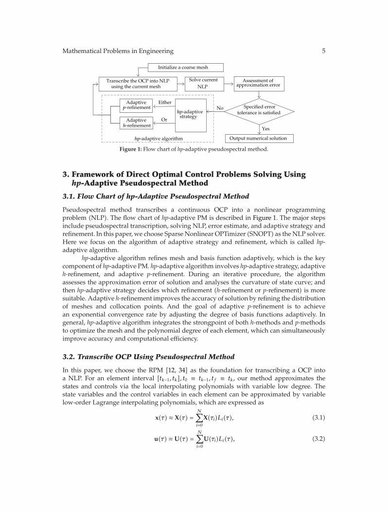
Figure 1: Flow chart of hp-adaptive pseudospectral method.
3. Framework of Direct Optimal Control Problems Solving Usinghp-Adaptive Pseudospectral Method
3.1. Flow Chart of hp-Adaptive Pseudospectral Method
Pseudospectral method transcribes a continuous OCP into a nonlinear programmingproblem (NLP). The flow chart of hp-adaptive PM is described in Figure 1. The major stepsinclude pseudospectral transcription, solving NLP, error estimate, and adaptive strategy andrefinement. In this paper, we choose Sparse Nonlinear OPTimizer (SNOPT) as theNLP solver.Here we focus on the algorithm of adaptive strategy and refinement, which is called hp-adaptive algorithm.
hp-adaptive algorithm refines mesh and basis function adaptively, which is the keycomponent of hp-adaptive PM. hp-adaptive algorithm involves hp-adaptive strategy, adaptiveh-refinement, and adaptive p-refinement. During an iterative procedure, the algorithmassesses the approximation error of solution and analyses the curvature of state curve; andthen hp-adaptive strategy decides which refinement (h-refinement or p-refinement) is moresuitable. Adaptive h-refinement improves the accuracy of solution by refining the distributionof meshes and collocation points. And the goal of adaptive p-refinement is to achievean exponential convergence rate by adjusting the degree of basis functions adaptively. Ingeneral, hp-adaptive algorithm integrates the strongpoint of both h-methods and p-methodsto optimize the mesh and the polynomial degree of each element, which can simultaneouslyimprove accuracy and computational efficiency.
3.2. Transcribe OCP Using Pseudospectral Method
In this paper, we choose the RPM [12, 34] as the foundation for transcribing a OCP intoa NLP. For an element interval [tk−1, tk], t0 ≡ tk−1, tf ≡ tk, our method approximates thestates and controls via the local interpolating polynomials with variable low degree. Thestate variables and the control variables in each element can be approximated by variablelow-order Lagrange interpolating polynomials, which are expressed as
x(τ) ≈ X(τ) =N∑
i=0
X(τi)Li(τ), (3.1)
u(τ) ≈ U(τ) =N∑
i=0
U(τi)Li(τ), (3.2)
6 Mathematical Problems in Engineering
where (τ1, . . . τN)are collocation points, plus the start point τ0 ≡ −1, N is the number ofcollocation points. Li(τ), (i = 0, 1, . . . ,N), is a basis of Lagrange polynomial with a variabledegree. Then differential constraint of (2.8) can be transcribed into the algebraically form
N∑
i=0
Li(τi)xi −tf − t0
2f(Xi,Ui, τ ; t0, tf
)= 0, (3.3)
where Xi = X(τi), Ui = U(τi), (i = 1, . . . ,N). The initial state X0 ≡ X(τ0), and terminal stateXf ≡ X(τf) satisfies Gauss quadrature formula
Xf ≡ X0 +tf − t0
2
N∑
i=1
ωif(Xi,Ui, τi; t0, tf
)= 0. (3.4)
Differentiating X(τ) in (3.1) with respect to τ , we get
dX(τ)dτ
≡ X(τ) =N∑
i=0
X(τi)Li(τ) =N∑
i=0
X(τi)dLi(τ)dτ
. (3.5)
The continuous objective function of (2.7) can be approximated via LGR quadrature
J ≡ φ(X0, t0,Xf , tf)+tf − t0
2
N∑
i=0
ωig(Xi,Ui, τ ; t0, tf
), (3.6)
whereωi is the weight coefficients of Gauss quadrature. And the boundary conditions of (2.9)is
ψ(X0, t0,Xf , tf
)= 0. (3.7)
Combining the state and control variances, the trajectory is constrained by
C(Xi,Ui, τi; t0, tf
) ≤ 0. (3.8)
Through the above process, a continuous Bolza OCP is transcribed into a limited dimensionalNLP.
3.3. Assessment of Approximation Error
In the iterative procedure, assessment of approximation error is not only a stopping criterion,but also useful information for adaptive refinement. If local solution on a mesh elementhas not satisfy the specified accuracy, then the distribution of collocation points needs tobe modified, either by increasing the polynomial degree on the element, or by redividing theelement.
Mathematical Problems in Engineering 7
The state and control variables are approximated by basis function polynomials. Forthe kth element interval [tk−1, tk] in mesh, (k = 1, 2, . . . , K), we firstly transform the intervalof variable t into the interval of τ ∈ [τ0, τf]. Then the approximation polynomials of terminalstate are given as
Xk0 = Xk−10 +N∑
i=0
f(Xi,Ui, τi; tk−1, tk)
= Xk−10 +∫ τf
τ0
X(τ)dτ −∫ τf
τ0
X(τ)dτ +N∑
i=0
f(Xi,Ui, τi; tk−1, tk)
= Xk0 −[∫ τf
τ0
(N∑
i=0
X(τi)Li(τ)
)
dτ −N∑
i=0
f(Xi,Ui, τi; tk−1, tk)
]
,
(3.9)
where N is the number of collocation points in the kth element, (i = 0, 1, . . . ,N). Hence thelocal error of the element is given as
Xk0 − Xk0 =∫ τf
τ0
(N∑
i=0
X(τi)Li(τ)
)
dτ −N∑
i=0
f(Xi,Ui, τi; tk−1, tk). (3.10)
Furthermore, we can define the absolute error of the kth element interval as
εk =1hk
∣∣∣∣∣
∫ τf
τ0
(N∑
i=0
X(τi)Li(τ)
)
dτ −N∑
i=0
f(Xi,Ui, τi; tk−1, tk)
∣∣∣∣∣, (3.11)
where hk = tk − tk−1 is the length of the kth element interval. And the maximum relative errorover all state variable components j of the differential equations is given by
η(k) = maxj
εkωj, (3.12)
where
ωj =1N
N∑
i=0
∣∣xj,i∣∣. (3.13)
ωj is the even value of the jth state variable on allN collocation points. η(k) is the maximumrelative error of all state variables on the kth element interval.
Let η be a specified accuracy tolerance for the discretized differential algebraicconstraints. If the maximum violation of the differential algebraic equations in the kthelement η(k) is less than η, then the approximation of the kth element is considered to satisfythe accuracy tolerance.
8 Mathematical Problems in Engineering
4. Multicriterion hp-Adaptive Strategy Design
The local approximation error estimator indicates the element which should be refined, butit does not indicate whether the element is better to refine by an h-refinement or by a p-refinement. It is no longer sufficient to guide the adaptive refinement. A method for makingthat determination is called hp-adaptive strategy. We learn the lesson of adaptive strategy inFEM. Based on the observation, we propose three classes of useful criterion for hp-adaptivestrategy: prior knowledge, intermediate error, and curvature.
First, the priori knowledge of solution regularity is useful for hp-adaptive strategy. Asone criterion, it guides a p-refinement on the smooth segments and an h-refinement nearsingularities or flections of state curve. For example, the linear elliptic partial differentialequations with smooth coefficients only have point singularities near corners of the boundaryand where boundary conditions change.
The priori knowledge-based criterion requires an estimator, which evaluates theregularity value of intermediate approximate solution. Here we define the regularity value asr. A method for estimating the local regularity of a solution on a given mesh was proposedin [33], it indicated that
r ≈ 1 + α, (4.1)
where α is the parameter of a priori estimate for the error. α can be obtained from the previouscomputation of the error estimator.
At the initial step of hp-adaptive strategy, the regularity value rk of approximatesolution on the kth element is readily available by initialization. Let p0
kand pk, respectively,
denote the initial degree and current degree of basis polynomial in the k element. If pk+2 ≤ rk,then p-refinement is performed, otherwise h-refinement is adopted. Furthermore, let p0k =r0k− 2 be an optimal choice for initial p-refinement.
Second, intermediate error can be adopted as a criterion for hp-adaptive strategy.Define an intermediate error
ηI = γη, (4.2)
where γ is a parameter generally ranging from 5 to 20, η is a specified error tolerance, forexample let η = 0.01 (1% error). An appropriate value of γ should make tradeoff between thecriterion of intermediate error and the criterion of curvature. From a lot of experimentations,we find that an adopted γ between 5 and 20 effects good complement of the multicriterions.
For the element k in mesh, if the estimated error η(k) > ηI , it needs detailed h-refinement. The criterion based on intermediate error should lead to distribute the error moreeven on every subinterval. It has been shown that the error is equidistributed over all thesubintervals for an optimal mesh using h-refinement [11]. Hence, an optimal h-adaptivemeshdistribution should simultaneously reduce the global error and distribute the local error ofeach element equably.
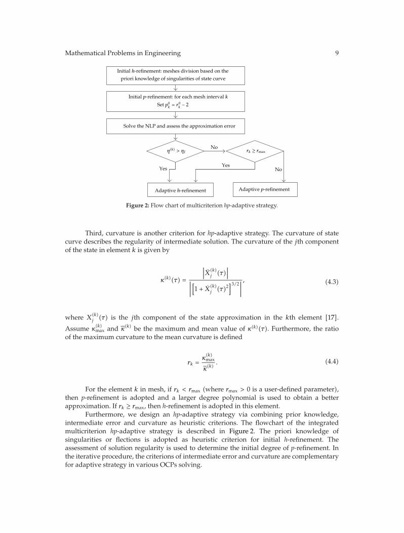
Mathematical Problems in Engineering 9
Initial h-refinement: meshes division based on thepriori knowledge of singularities of state curve
Adaptive h-refinement Adaptive p-refinement
Initial p-refinement: for each mesh interval k
Solve the NLP and assess the approximation error
No
No
YesYes
Set p0k= r0
k− 2
η(k) > ηI rk ≥ rmax
Figure 2: Flow chart of multicriterion hp-adaptive strategy.
Third, curvature is another criterion for hp-adaptive strategy. The curvature of statecurve describes the regularity of intermediate solution. The curvature of the jth componentof the state in element k is given by
κ(k)(τ) =
∣∣∣X(k)j (τ)
∣∣∣∣∣∣∣[1 + X(k)
j (τ)2]3/2∣∣∣∣
, (4.3)
where X(k)j (τ) is the jth component of the state approximation in the kth element [17].
Assume κ(k)max and κ(k) be the maximum and mean value of κ(k)(τ). Furthermore, the ratioof the maximum curvature to the mean curvature is defined
rk =κ(k)max
κ(k). (4.4)
For the element k in mesh, if rk < rmax (where rmax > 0 is a user-defined parameter),then p-refinement is adopted and a larger degree polynomial is used to obtain a betterapproximation. If rk ≥ rmax, then h-refinement is adopted in this element.
Furthermore, we design an hp-adaptive strategy via combining prior knowledge,intermediate error and curvature as heuristic criterions. The flowchart of the integratedmulticriterion hp-adaptive strategy is described in Figure 2. The priori knowledge ofsingularities or flections is adopted as heuristic criterion for initial h-refinement. Theassessment of solution regularity is used to determine the initial degree of p-refinement. Inthe iterative procedure, the criterions of intermediate error and curvature are complementaryfor adaptive strategy in various OCPs solving.
10 Mathematical Problems in Engineering
5. Integrated Multicriterion hp-Adaptive Algorithm Procedure
In this section, we depict an integrated multicriterion hp-adaptive algorithm for a nonlinearcontinuous OCP with K intervals. The algorithm mainly includes six procedures.
Step 1 (initialization). Firstly, the error tolerance η is specified, for example η = 0.01 (1%error). Then the intermediate error ηI is specified, for example, ηI = 0.1. And rmax is specified,for example rmax = 8.
Consider the initial h-refinement for each state equation, if the equation is a piecewisefunction, the initial h-refinement is located at the switch points of piecewise function; ifthere is a priori knowledge of singularities or flections of state curve, it guides the meshesdivision also. If there is no information about switch points or singularities, a coarse initialh-refinement is made with uniform mesh element size h0. The discrete approximation ineach element is defined by the set of Legendre-Gauss-Radau points. And for the initial p-refinement, the polynomial-order of kth element is determined via the assessment of localsolution regularity, it is given as p0
k= r0
k− 2.
Step 2 (solve the NLP using the current mesh). The problem is transcribed into the NLPon the current mesh, and then solving the NLP using sequential quadratic programming(SQP). A posteriori error estimator is used to estimate the approximation errors for theintermediate solution on each element, which is described in Section 3.3. The accuracy of theapproximation in each element is assessed by calculating the differential-algebraic constraintson the collocation points.
Begin: For k = 1, 2, . . . , K.
Step 3. If η(k) ≤ η, then continue (proceed to next k + 1 element). η(k) is the approximationerror of the kth element in mesh.
Step 4 (adaptive h-refinement). If either η(k) > ηI , or rk ≥ rmax, then h-refine the kth element.h-refinement keeps p = p0 fixed and adaptively constructs elements with varying size. Itmaintains refinement until the solution achieves the intermediate error ηI and curvature ratiork < rmax. The new number of element intervals is computed by formula
nk =
⌈
log10
(η(k)
η
)
+ ch × loge
(η(k)
ηI
)⌉
=
⌈
log10
(η(k)
η
)
+ ch × loge10 × log10
(η(k)
ηI
)⌉
=
⎡
⎢⎢⎢log10
(η(k)
η
)
+ log10
(η(k)
ηI
)ch×loge10⎤
⎥⎥⎥
=
⎡
⎢⎢⎢log10
⎛
⎝(η(k)
η
)
×(η(k)
ηI
)ch×loge10⎞
⎠
⎤
⎥⎥⎥,
(5.1)
Mathematical Problems in Engineering 11
where η(k)/η is the ratio between current estimative maximum error and the specifiederror tolerance, η(k)/ηI is the ratio between current estimative maximum error and theintermediate error, and �•� is the operator that rounds to the next integer. ch is an integerconstant as a parameter for adjusting iterative speed, for example, ch = 2. If there is someprior knowledge about state curve, ch can be adjusted for flections.
Formula (5.1) determines a dissatisfactory element interval should be subdivided intohow many subelements by h-refinement. The formula is based on two ratios. The first partdepicts the approximation degree from the current error to the specified error tolerance; andthe second part indicates the approximation degree from the current error to the intermediateerror. They are calculated by the log operation, because h-refinement is hoped to attain anexponential convergence for the nonsmooth segment of function. The choices of logarithmare based on the quantity relation of the ratios. ch controls the growth in the number ofelement intervals. If ch is sufficiently large, the algorithm will use less iteration to convergeto an acceptable solution, but the number of collocation points may increase quickly betweeniterations. If ch is small, the mesh will increase slowly, but the algorithm may require manyiterations. An appropriate value of ch should make tradeoff between h-refinement and p-refinement.
The locations of the new required-elements are determined using the integral of acurvature density function in a manner similar to that given in [35]. Specifically, let ρ(τ)be the density function given by
ρ(τ) = cκ(τ)1/3, (5.2)
where c is a constant to satisfy
∫+1
−1ρ(ζ)dζ = 1. (5.3)
The density function expressed by (5.2) is a probability density function (pdf)with fractionalpower-laws. Here we adopt 1/3 power in the function. In fact, from the point of view ofpower-laws in stochastic processes and/or fractal time series, 1/3 power is a typical heavy-tailed case. By heavy-tailed we mean that the density ρ(τ) decays slowly. And heavy-tailedpdfs imply that τ is in wild randomness due to infinite or very large variance [36].
Let F(τ) be the cumulative distribution function given by
F(τ) =∫ τ
−1ρ(ζ)dζ. (5.4)
The nk new mesh points are chosen by
F(τ) =i − 1nk
, 1 ≤ i ≤ nk + 1. (5.5)
Finally, it is noted that if nk = 1, then no subintervals are created. Therefore, the minimumvalue for nk is 2.
12 Mathematical Problems in Engineering
Step 5 (adaptive p-refinement). p-refinement keeps mesh and the size of elements fixed. Itadjusts the degree of polynomials on each element until the final error is satisfied. The degreeof polynomial pk on the kth element is determined by
pk = pk +
⌈
log10
(η(k)
η
)
+ loge
(η(k)
ηI
)⌉
= pk +
⌈
log10
(η(k)
η
)
+ loge10 × log10
(η(k)
ηI
)⌉
= pk +
⎡
⎢⎢⎢log10
(η(k)
η
)
+ log10
(η(k)
ηI
)loge10⎤
⎥⎥⎥
= pk +
⎡
⎢⎢⎢log10
⎛
⎝(η(k)
η
)
×(η(k)
ηI
)loge10⎞
⎠
⎤
⎥⎥⎥,
(5.6)
where pk is the initial degree of polynomial on this element. The growth in the polynomialdegree is related to the log of the error ratio; because of a smooth function always exhibitsexponential convergence in pseudospectral method.
End: For k = 1, 2, . . . , K.
Step 6 (return to Step 2). Our hp-adaptive algorithm integrates prior knowledge, intermediateerror, and curvature for adaptive strategy and refinement, which is fit for smooth ornonsmooth problem. The illustration and comparison of our algorithm will be given by theexamples in next section.
Remark 5.1. The accuracy and efficiency of the PMs for solving numerical optimal controlproblems have motivated the forefront of research. For continuous and smooth problems,pseudospectral knots and Gaussian quadrature rules are used to generate a natural spectralmesh that is dense near the points of interest. For nonsmooth problems, how to locateswitches, kinks, corners, and other discontinuities is a challenge for solving practical OCPs.In our hp-adaptive algorithm procedure, adaptive h-refinement is devised to locate the knotswhere the solution is subject to sudden changes, as in points of discontinuity. In fact, from thepoint of view of stochastic processes, the curve of solution is higher order discontinuities inthe control time history. According to its statistic properties, it is fractal time series. In general,fractal time series have a heavy-tailed probability distribution function, a slowly decayedautocorrelation function (ACF), and a power spectrum function (PSD) of 1/f type [37]. Inour approach, we design the density function expressed by (5.2). We adopt the 1/3 power, thedensity decays slowly, accordingly, heavy-tailed density. In our research of the practical OCPin engineering, such as aerospace engineering or mechanical engineering, the nonsmoothnessand discontinuities are attributed to the differential dynamic and the constraint of system.The output or response of a differential system can be considered as a fractal time series[37, 38]. The density functions for mesh refinement in numerical optimal control are aninstance of power-law-type pdf. The key problem of h-refinement is to find an appropriatedensity function. We mean that an appropriate choice of density function may help increasethe accuracy of the solution and improve numerical robustness. Hence the theory of fractal
Mathematical Problems in Engineering 13
time series and power-laws would guide the choice. Li gives a tutorial review about fractaltime series [37]. The locally weak stationarity of modified multifractional Gaussian noiseis discussed in [39], which presents a set of stationary ranges. One-dimensional randomfunction with long memory is introduced to model the sea level fluctuation [40]. Topicsin power-laws are paid attention too, see for example, the contribution of approximatingideal filters by systems of fractional order in [41], the work of addressing power laws incyber-physical networking systems in [36], the contribution of simplicial approach to fractalstructures by Cattani et al. in [42], and the work of Li et al. in [38].
6. Numerical Examples
In this section, we present two numerical examples to illustrate the convergence rate andthe applicability of the proposed method. The first example is a hypersensitive OCP, whichsolution has dramatic change on the “take-off” and “landing” segments. And the secondexample is a reusable launch vehicle re-entry trajectory optimization. The experimentationscompare three algorithms: GPM [12], hp-adaptive PM based on curvature [17], and ourintegrated multicriterion hp-adaptive PM. For conciseness, the three algorithms are denotedby p, hp(1), hp(2), respectively. All CPU time recorded in table is whole time of iteration,which includes the time required to solve the NLP and the time required to refine the meshes.The program of these algorithms is expanded from open-source software GPOPS [43]. Thetranscribed NLP is solved by SNOPT [44, 45], using a 2.4-GHz Core 2 Duo, 2G DDR RAMpersonal computer with MATLAB R2009b. For all examples, the following values are chosenfor the parameters described in Section 4: rmax = 8 and γ = 10. In hp(1) and hp(2), themaximumnumber of collocation points on each mesh is 20, and the upper bound of iteration times is20.
Example 6.1. Consider the following hypersensitive OCP adapted from [46]. It is aHamiltonian boundary value OCP in long time interval. Minimize the cost function
J =12
∫ tf
0
(x2 + u2
)dt, (6.1)
subject to the dynamic constraint
x = −x3 + u, (6.2)
and the boundary conditions
x(0) = 1.5, x(tf)= 1, (6.3)
where tf is fixed. This problem has a “take-off”, “cruise”, and “landing” structure where allof the interesting behaviors occur in the “take-off” and “landing” segments. In this example,tf = 1000.
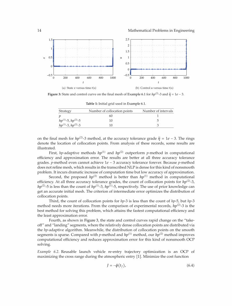
The specification of initial grid is listed in Table 1. The efficiency and accuracy ofvarious methods are listed in Table 2. Figure 3 shows the state and control curve of solution
14 Mathematical Problems in Engineering
−0.5
0
0.5
1
1.5x
0 200 400 600 800 1000
t
(a) State x versus time t(s)
0 200 400 600 800 1000−0.5
0
0.5
1
1.5
2
2.5
t
u
(b) Control u versus time t(s)
Figure 3: State and control curve on the final mesh of Example 6.1 for hp(2)-3 and η = 1e − 3.
Table 1: Initial grid used in Example 6.1.
Strategy Number of collocation points Number of intervalsp 60 1hp(1)-5, hp(2)-5 10 5hp(1)-3, hp(2)-3 10 3
on the final mesh for hp(2)-3 method, at the accuracy tolerance grade η = 1e − 3. The ringsdenote the location of collocation points. From analysis of these records, some results areillustrated.
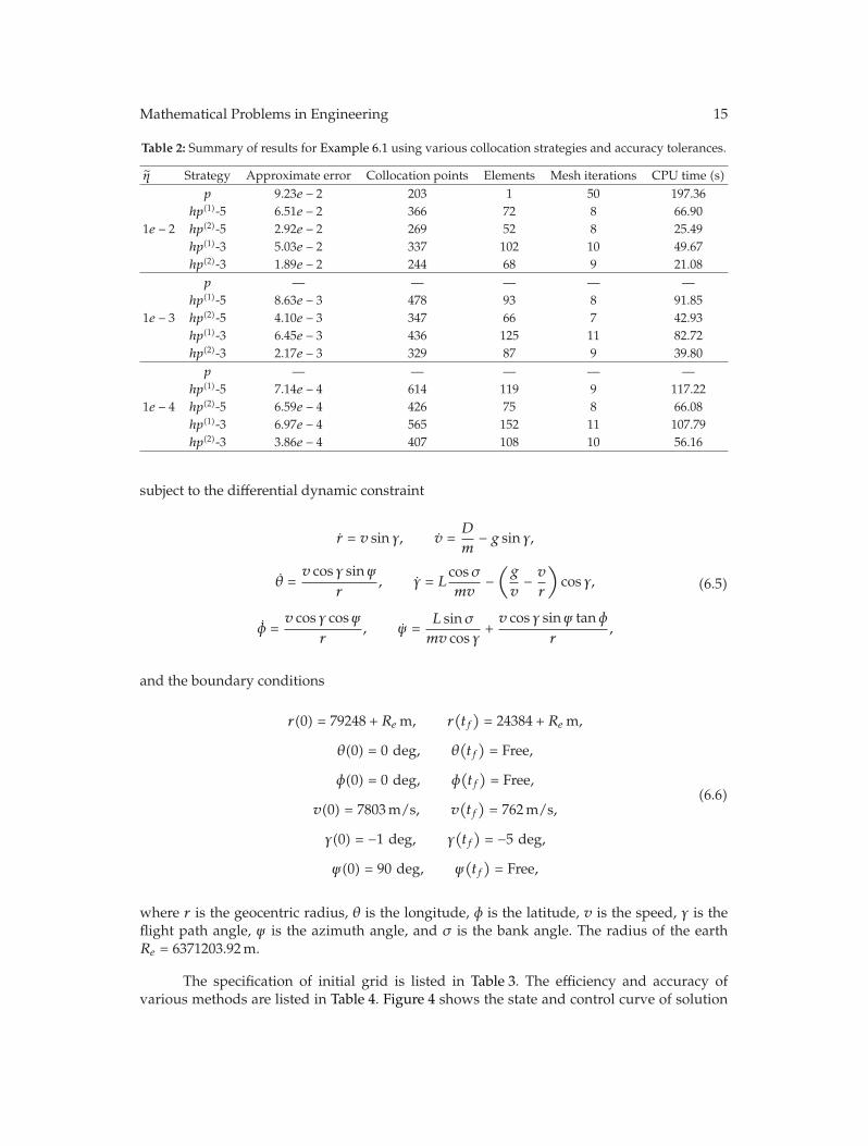
First, hp-adaptive methods hp(1) and hp(2) outperform p-method in computationalefficiency and approximation error. The results are better at all three accuracy tolerancegrades. p-method even cannot achieve 1e − 3 accuracy tolerance forever. Because p-methoddoes not refinemesh, which results in the transcribedNLP is dense for this kind of nonsmoothproblem. It incurs dramatic increase of computation time but low accuracy of approximation.
Second, the proposed hp(2) method is better than hp(1) method in computationalefficiency. At all three accuracy tolerance grades, the count of collocation points for hp(2)-3,hp(2)-5 is less than the count of hp(1)-3, hp(1)-5, respectively. The use of prior knowledge canget an accurate initial mesh. The criterion of intermediate error optimizes the distribution ofcollocation points.
Third, the count of collocation points for hp-3 is less than the count of hp-5, but hp-3method needs more iterations. From the comparison of experimental records, hp(2)-3 is thebest method for solving this problem, which attains the fastest computational efficiency andthe least approximation error.
Fourth, as shown in Figure 3, the state and control curves rapid change on the “take-off” and “landing” segments, where the relatively dense collocation points are distributed viathe hp-adaptive algorithm. Meanwhile, the distribution of collocation points on the smoothsegments is sparse. Compared with p-method and hp(1) method, our hp(2) method improvescomputational efficiency and reduces approximation error for this kind of nonsmooth OCPsolving.
Example 6.2. Reusable launch vehicle re-entry trajectory optimization is an OCP ofmaximizing the cross range during the atmospheric entry [1]. Minimize the cost function
J = −φ(tf), (6.4)
Mathematical Problems in Engineering 15
Table 2: Summary of results for Example 6.1 using various collocation strategies and accuracy tolerances.
η Strategy Approximate error Collocation points Elements Mesh iterations CPU time (s)p 9.23e − 2 203 1 50 197.36
hp(1)-5 6.51e − 2 366 72 8 66.901e − 2 hp(2)-5 2.92e − 2 269 52 8 25.49
hp(1)-3 5.03e − 2 337 102 10 49.67hp(2)-3 1.89e − 2 244 68 9 21.08p — — — — —
hp(1)-5 8.63e − 3 478 93 8 91.851e − 3 hp(2)-5 4.10e − 3 347 66 7 42.93
hp(1)-3 6.45e − 3 436 125 11 82.72hp(2)-3 2.17e − 3 329 87 9 39.80p — — — — —
hp(1)-5 7.14e − 4 614 119 9 117.221e − 4 hp(2)-5 6.59e − 4 426 75 8 66.08
hp(1)-3 6.97e − 4 565 152 11 107.79hp(2)-3 3.86e − 4 407 108 10 56.16
subject to the differential dynamic constraint
r = v sin γ, v =D
m− g sin γ,
θ =v cos γ sinψ
r, γ = L
cosσmv
−(g
v− v
r
)cos γ,
φ =v cos γ cosψ
r, ψ =
L sinσmv cos γ
+v cos γ sinψ tanφ
r,
(6.5)
and the boundary conditions
r(0) = 79248 + Rem, r(tf)= 24384 + Rem,
θ(0) = 0 deg, θ(tf)= Free,
φ(0) = 0 deg, φ(tf)= Free,
v(0) = 7803m/s, v(tf)= 762m/s,
γ(0) = −1 deg, γ(tf)= −5 deg,
ψ(0) = 90 deg, ψ(tf)= Free,
(6.6)
where r is the geocentric radius, θ is the longitude, φ is the latitude, v is the speed, γ is theflight path angle, ψ is the azimuth angle, and σ is the bank angle. The radius of the earthRe = 6371203.92m.
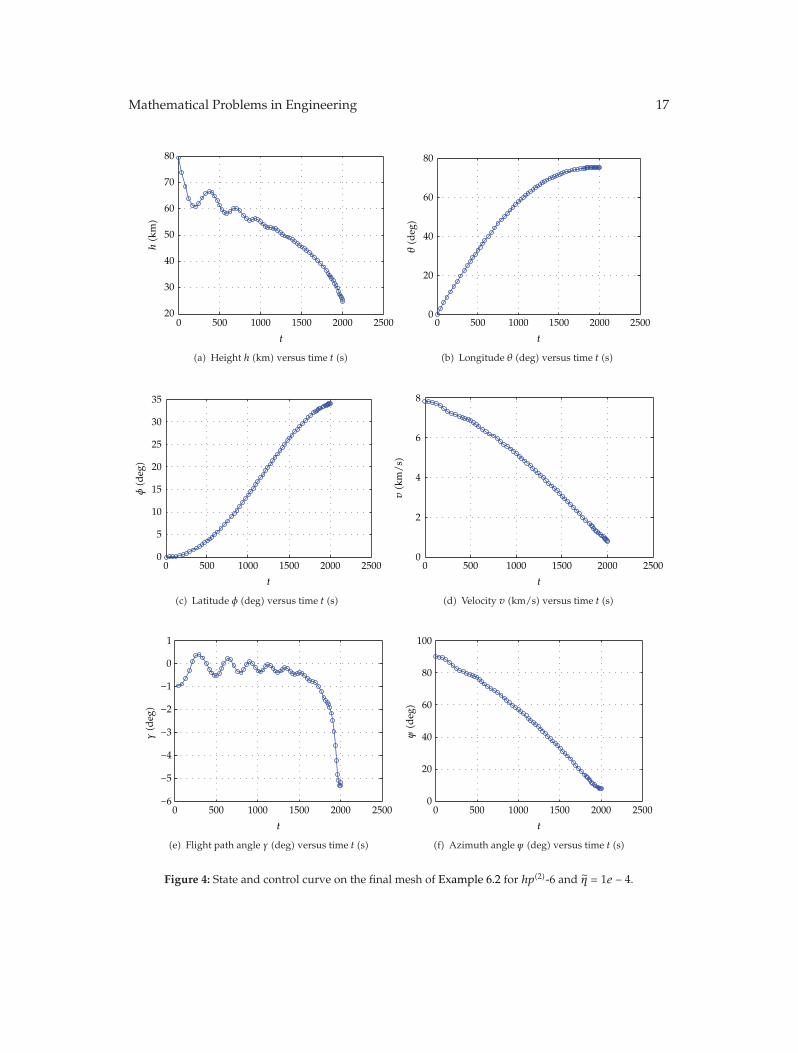
The specification of initial grid is listed in Table 3. The efficiency and accuracy ofvarious methods are listed in Table 4. Figure 4 shows the state and control curve of solution
16 Mathematical Problems in Engineering
Table 3: Initial grid used in Example 6.2.
Strategy Number of collocation points Number of intervalsp 50 1hp(1)-6, hp(2)-6 10 6hp(1)-4, hp(2)-4 10 4
Table 4: Summary of results for Example 6.2 using various collocation strategies and accuracy tolerances.
η Strategy Approximate error Collocation points Elements Mesh iterations CPU time (s)p 7.61e − 3 58 1 4 70.88
hp(1)-6 5.12e − 3 90 18 2 19.551e − 3 hp(2)-6 3.55e − 3 70 12 3 18.05
hp(1)-4 6.81e − 3 113 32 4 32.55hp(2)-4 4.19e − 3 83 18 4 19.66p 9.17e − 4 75 1 12 88.94
hp(1)-6 4.08e − 4 151 29 6 33.761e − 4 hp(2)-6 3.23e − 4 122 21 4 24.89
hp(1)-4 7.99e − 4 202 56 6 63.71hp(2)-4 5.83e − 4 153 34 4 40.24p 9.74e − 5 90 1 16 99.50
hp(1)-6 8.02e − 5 214 40 6 63.641e − 5 hp(2)-6 7.50e − 5 183 32 5 53.44
hp(1)-4 8.93e − 5 293 70 5 89.46hp(2)-4 7.69e − 5 251 51 5 84.88
on the final mesh for hp(2)-6 method, at the accuracy tolerance grade η = 1e− 4. The state andcontrol curves are relatively smooth for this example. From analysis of these records, someresults are illustrated.
First, hp-adaptive methods hp(1) and hp(2) are similar or better than p-method in thisexample. p-method can achieve 1e − 5 accuracy tolerance and has the fewest number ofcollocation points, but it needs much iteration. The computational time of p-method is longerthan hp-adaptive methods. The low computational efficiency of p-method is due to the factthat the transcribed NLP is dense.
Second, our hp(2) method outperforms hp(1) method in computational efficiency. Thecount of collocation points for hp(2) is less than the count of hp(1) at three accuracy tolerancegrades. The comparison illustrates that the distribution of collocation points via hp(2) is betterthan the distribution via hp(1).
Third, the count of collocation points for hp-6 is less than the count of hp-4. Based onthe comparison of experimental records, hp(2)-6 is the best method for solving this problem,which has the fastest computational efficiency and the least approximation error. In general,our method is feasible and improves computational efficiency for this kind of smooth OCPsolving.
Remark 6.3. The results of examples highlight several points of p-methods and hp-adaptivemethods. p-methods are fit for solving problems which their solutions are smooth. hp-adaptive methods perform similarly or better to p-methods for smooth problems. Fornonsmooth problems, p-methods cannot accurately capture the discontinuities and rapid
Mathematical Problems in Engineering 17
20
30
40
50
60
70
80h(k
m)
0 500 1000 1500 2000 2500
t
(a) Height h (km) versus time t (s)
20
40
60
80
0 500 1000 1500 2000 25000
t
θ(d
eg)
(b) Longitude θ (deg) versus time t (s)
0 500 1000 1500 2000 2500
t
0
5
10
15
20
25
30
35
φ(d
eg)
(c) Latitude φ (deg) versus time t (s)
0 500 1000 1500 2000 2500
t
0
2
4
6
8v(k
m/
s)
(d) Velocity v (km/s) versus time t (s)
0 500 1000 1500 2000 2500
t
−6
−5
−4
−3
−2
−1
0
1
γ(d
eg)
(e) Flight path angle γ (deg) versus time t (s)
0 500 1000 1500 2000 2500
t
0
20
40
60
80
100
ψ(d
eg)
(f) Azimuth angle ψ (deg) versus time t (s)
Figure 4: State and control curve on the final mesh of Example 6.2 for hp(2)-6 and η = 1e − 4.
18 Mathematical Problems in Engineering
changes in the trajectory. They only achieve low-accuracy even with much iteration. Whena high-accuracy tolerance is required to satisfy, hp-adaptive methods are the likeliestcandidates. They transcribe the OCPs into the NLPs with computational sparsity, which leadsto the reduction of execution time. Compared with hp-adaptive PM based on curvature,our method is more efficient in the convergence rate; meanwhile the solutions achieve acomparable or better accuracy. The prior knowledge and the criterion of intermediate errorleverage the enhancement of performance. The prior knowledge guides an accurate initialmesh, and the criterion of intermediate error optimizes the distribution of collocation points.
7. Conclusions
PMs become increasingly popular for direct OCPs solving in the engineering area. It ischallenging to improve the convergence rate, the solution accuracy, and the applicabilityof algorithms, especially for nonsmooth problems. In this paper, we proposed a novelmethod which integrates multicriterion to hp-adaptive PM, in order to further improvethe performance of computation and approximation. For this purpose, we first devised anOCP solving framework of hp-adaptive PM. We then designed a multicriterion hp-adaptivestrategy which introduces prior knowledge, intermediate error, and curvature as usefulcriterions for adaptive refinement. The criterions of intermediate error and curvature werecomplementary for adaptive strategy in various OCPs solving. We last proposed an iterativeprocedure for solving general nonlinear OCPs. Our method converged by increasing thepolynomial degree in the smooth segments of a solution; meanwhile it adaptively refined themesh for the nonsmooth segments in an efficient way. Results from examples showed thatour method significantly outperforms hp-adaptive PM based on curvature and effectivelyimproves the convergence rate of computation and the accuracy of solution. Meanwhile, itenhances the applicability of hp-adaptive PMs for solving various OCPs.
For the future work, we will evaluate the performance of the proposed method usingmore OCPs in the engineering area. We will also try to exploit other valuable criterions forhp-adaptive method, which may further improve the convergence rate and the applicabilityof PMs. In addition, the choices of initial grid of PMs and the values of parameters (γ ,rmax, and ch) will be further researched for various problems. Different problem types willneed dissimilar parameters for fast solving. Another topic is applying fractal time series andpower-laws to guide the choice of density function for various problems. This point itself isan issue worth discussing in our future work.
Appendix
Basis of the Pseudospectral Method
Much of the details of pseudospectral methods (PMs) are extensively described elsewhere[2, 15, 16, 34]; here, we briefly summarize the basis of the PM. The basic principle of a PM isto solve the continuous optimal control problem (OCP) by discretizing it to the NLP problem.The whole process mainly includes three steps. First, the horizon of a continuous OCP ismapped to a finite spectral interval [−1, 1]. Second, a PM is applied to discretize the problem.The discretized problem generates a sequence of approximate problems parameterized bythe size of the grid. In the third step, each discretized problem in this sequence is solvedby a globally convergent sequential quadratic programming (SQP) technique. In the PMs,
Mathematical Problems in Engineering 19
the functions are approximated by Lagrange interpolating polynomials of orderN in whichinterpolation occurs at Gaussian quadrature points. There are three different families of Gaussquadrature points known as Legendre-Gauss, Legendre-Gauss-Radau, and Legendre-Gauss-Lobatto. Gauss PM (GPM) [12], Radau PM (RPM) [13], and Lobatto PM (LPM) [14] arethe three most well-developed PMs. The collocation points of them are based on accuratequadrature rules. Their basis functions are typically Chebyshev or Lagrange polynomial.
Here we describe the procedure of GPM as an illustrative method. The GPMapproximates the state using a basis of global interpolating Lagrange polynomials. Theseglobal polynomials are based on a set of discrete Legendre-Gauss (LG) points across theinterval.
The standard interval considered here is denoted as τ ∈ [−1, 1]. By using a lineartransformation, the actual time t can be expressed as a function of τ via
t =
[(tf − t0
)τ +(tf + t0
)]
2, τ =
2t(tf − t0
) −(tf + t0
)
(tf − t0
) , (A.1)
where t0 and tf stand for the initial and final time, respectively.The state is approximated using a basis ofN + 1 Lagrange interpolating polynomials,
Li(τ) (i = 0, . . . ,N), as follows:
x(τ) ≈ X(τ) =N∑
i=0
X(τi)Li(τ), (A.2)
where
Li(τ) =N∏
j=0,j /= i
τ − τjτi − τj , (A.3)
where τi, (i = 0, . . . ,N) are the LG points belonging to the set.An approximation to the control, U(τ), is formed with a basis of N Lagrange
interpolating polynomials, Li(τ) (i = 1, . . . ,N), as follows:
u(τ) ≈ U(τ) =N∑
i=1
U(τi)Li(τ). (A.4)
The differential dynamic constraints should be posed to ensure that the entire discretestate satisfies the dynamic equations. The left-hand side of the dynamic equations isapproximated by differentiating the state approximation of (A.1) at the LG points as follows:
x(τk) ≈ X(τk) =N∑
i=0
X(τi)Li(τk) =N∑
i=0
DkiX(τi), (k = 1, . . . ,N). (A.5)
20 Mathematical Problems in Engineering
The differentiation matrix,D ∈ RN×(N+1), can be determined offline from dynamic equations:
Dki = Li(τk) =
⎧⎪⎪⎪⎪⎨
⎪⎪⎪⎪⎩
(1 + τk)PN(τk) + PN(τk)(τk − τi)
[(1 + τi)PN(τi) + PN(τi)
] , i /= k
(1 + τi)PN(τi) + 2PN(τi)2[(1 + τi)PN(τi) + PN(τi)
] , i = k.
(A.6)
The N collocation equations require (A.5) to be equal to the right-hand side of thedynamic equations at the collocation points:
N∑
i=0
DkiX(τi) −tf − t0
2f(X(τk), U(τk), τk; t0, tf
)= 0, (k = 1, . . . ,N). (A.7)
As it is shown shortly, collocating strictly on the interior of the interval leads to aunique mathematical equivalence used to approximate the costate.
Combining the state and control variances, the constraints are discretized as follows:
C(Xk,Uk, τk; t0, tf
) ≤ 0. (A.8)
Lastly, the integral term in the cost functional can be approximated with a Gaussquadrature as follows:
J = Φ(X0, t0, Xf , tf
)+tf − t0
2
N∑
k=1
ωkg(Xk,Uk, τk; t0, tf
), (A.9)
where ωk is the weight coefficient of Gauss quadrature.Through the above process, a continuous OCP is transcribed into a limited
dimensional NLP. The formulation is as follows:
min F(y)
s.t. gj(y) ≤ 0, j = 1, 2, . . . , p
hk(y) = 0, k = 1, 2, . . . , q.
(A.10)
The transcribed NLP can be solved by well-developed algorithms, such as SQP,interior point method, particle swarm optimization and so on.
Acknowledgments
Great thanks go to the reviewers for valuable comments on our revision of the paper. Thiswork was supported by the National Natural Science Foundation of China (61005077),the National Basic Research Program of China (6138101001), and the National DefenseFoundation of China (403060103).
Mathematical Problems in Engineering 21
References
[1] J. T. Betts, Practical Methods for Optimal Control and Estimation Using Nonlinear Programming, Advancesin Design and Control, SIAM Press, Philadelphia, Pa, USA, 2nd edition, 2009.
[2] D. Garg, M. Patterson, W. W. Hager, A. V. Rao, D. A. Benson, and G. T. Huntington, “A unifiedframework for the numerical solution of optimal control problems using pseudospectral methods,”Automatica, vol. 46, no. 11, pp. 1843–1851, 2010.
[3] K.W and B. N, “Pseudospectral optimal control theorymakes debut flight-saves NASA $1M in under3 hrs,” SIAM News, vol. 40, no. 7, pp. 1–2, 2007.
[4] M. Li, “An optimal controller of an irregular wave maker,” Applied Mathematical Modelling, vol. 29, no.1, pp. 55–63, 2005.
[5] S. Castellucci, M. Carlini, M. Guerrieri, and T. Honorati, “Stability and control for energy productionparametric dependence,” Mathematical Problems in Engineering, vol. 2010, Article ID 842380, 21 pages,2010.
[6] M. Soler, A. Olivares, and E. Staffetti, “Hybrid optimal control approach to commercial aircrafttrajectory planning,” Journal of Guidance, Control, and Dynamics, vol. 33, no. 3, pp. 985–991, 2010.
[7] L. Xie, P. Yang, T. Yang et al., “Dual-EKF-based real-time celestial navigation for lunar rover,”Mathematical Problems in Engineering, vol. 2012, Article ID 578719, 16 pages, 2012.
[8] S. H. Pourtakdoust, M. Kiani, and A. Hassanpour, “Optimal trajectory planning for flight throughmicroburst wind shears,” Aerospace Science and Technology, vol. 15, no. 7, pp. 567–576, 2011.
[9] M. Li, “An iteration method to adjusting random loading for a laboratory fatigue test,” InternationalJournal of Fatigue, vol. 27, no. 7, pp. 783–789, 2005.
[10] I. Babuska and M. Suri, “The p and h-p versions of the finite element method, basic principles andproperties,” SIAM Review, vol. 36, no. 4, pp. 578–632, 1994.
[11] W. F. Mitchell and M. A. McClain, “A survey of hp-adaptive strategies for elliptic partial differentialequations,” in Recent Advances in Computational and Applied Mathematics, pp. 227–258, Springer,Amsterdam, The Netherlands, 2011.
[12] D. A. Benson, G. T. Huntington, T. P. Thorvaldsen, and A. V. Rao, “Direct trajectory optimization andcostate estimation via an orthogonal collocation method,” Journal of Guidance, Control, and Dynamics,vol. 29, no. 6, pp. 1435–1440, 2006.
[13] D. Garg, M. A. Patterson, C. L. Darby et al., “Direct trajectory optimization and costate estimation offinite-horizon and infinite-horizon optimal control problems using a Radau pseudospectral method,”Computational Optimization and Applications, vol. 49, no. 2, pp. 335–358, 2011.
[14] G. Elnagar, M. A. Kazemi, and M. Razzaghi, “The pseudospectral Legendre method for discretizingoptimal control problems,” IEEE Transactions on Automatic Control, vol. 40, no. 10, pp. 1793–1796, 1995.
[15] B. Fornberg, A Practical Guide to Pseudospectral Methods, Cambridge Monographs on Applied andComputational Mathematics, Cambridge University Press, New York, NY, USA, 1998.
[16] Q. Gong, F. Fahroo, and I. M. Ross, “Spectral algorithm for pseudospectral methods in optimalcontrol,” Journal of Guidance, Control, and Dynamics, vol. 31, no. 3, pp. 460–471, 2008.
[17] C. L. Darby, W. W. Hager, and A. V. Rao, “Direct trajectory optimization using a variable low-orderadaptive pseudospectral method,” Journal of Spacecraft and Rockets, vol. 48, no. 3, pp. 433–445, 2011.
[18] C. L. Darby, W.W. Hager, and A. V. Rao, “An hp-adaptive pseudospectral method for solving optimalcontrol problems,” Optimal Control Applications & Methods, vol. 32, no. 4, pp. 476–502, 2011.
[19] A. K. Patra, A. Laszloffy, and J. Long, “Data structures and load balancing for parallel adaptive hpfinite-element methods,” Computers andMathematics with Applications, vol. 46, no. 1, pp. 105–123, 2003.
[20] L. Demkowicz, W. Rachowicz, and Ph. Devloo, “A fully automatic hp-adaptivity,” Journal of ScientificComputing, vol. 17, no. 1–4, pp. 117–142, 2002.
[21] L. Demkowicz, “Computing with hp-adaptive finite elements,” inOne and Two Dimensional Elliptic andMaxwell Problems, Chapman & Hall/CRC, Boca Raton, Fla, USA, 2007.
[22] P. Solın, J. Cerveny, and I. Dolezel, “Arbitrary-level hanging nodes and automatic adaptivity in thehp-FEM,”Mathematics and Computers in Simulation, vol. 77, no. 1, pp. 117–132, 2008.
[23] R. Tews andW. Rachowicz, “Application of an automatic hp adaptive finite element method for thin-walled structures,” Computer Methods in Applied Mechanics and Engineering, vol. 198, no. 21-26, pp.1967–1984, 2009.
[24] P. Solın and M. Kuraz, “Solving the nonstationary Richards equation with adaptive hp-FEM,”Advances in Water Resources, vol. 34, no. 9, pp. 1062–1081, 2011.
[25] A. Szymczak, A. Paszynska, M. Paszynski et al., “Anisotropic 2D mesh adaptation in hp-adaptiveFEM,” Procedia Computer Science, vol. 4, pp. 1818–1827, 2011.
22 Mathematical Problems in Engineering
[26] L. Galvao, M. Gerritsma, and B. D. Maerschalck, “hp-adaptive least squares spectral element methodfor hyperbolic partial differential equations,” Journal of Computational and Applied Mathematics, vol.215, no. 2, pp. 409–418, 2008.
[27] H. Ben Dhia, L. Chamoin, J. T. Oden, and S. Prudhomme, “A new adaptive modeling strategy basedon optimal control for atomic-to-continuum coupling simulations,” Computer Methods in AppliedMechanics and Engineering, vol. 200, no. 37–40, pp. 2675–2696, 2011.
[28] J. T. Oden and S. Prudhomme, “Control of modeling error in calibration and validation processes forpredictive stochastic models,” International Journal for Numerical Methods in Engineering, vol. 87, no.1–5, pp. 262–272, 2011.
[29] C. A. Dorao and H. A. Jakobsen, “hp-adaptive least squares spectral element method for populationbalance equations,” Applied Numerical Mathematics, vol. 58, no. 5, pp. 563–576, 2008.
[30] C. A. Dorao, M. Fernandino, H. A. Jakobsen, and H. F. Svendsen, “hp-Adaptive spectral elementsolver for reactor modeling,” Chemical Engineering Science, vol. 64, no. 5, pp. 904–911, 2009.
[31] Z. Lu, “Adaptive mixed finite element methods for parabolic optimal control problems,”MathematicalProblems in Engineering, vol. 2011, Article ID 217493, 21 pages, 2011.
[32] J. T. Oden and A. Patra, “A parallel adaptive strategy for hp finite element computations,” ComputerMethods in Applied Mechanics and Engineering, vol. 121, no. 1–4, pp. 449–470, 1995.
[33] M. Ainsworth and B. Senior, “An adaptive refinement strategy for hp-finite element computations,”Applied Numerical Mathematics, vol. 26, no. 1-2, pp. 165–178, 1998.
[34] G. T. Huntington, Advancement and Analysis of a Gauss Pseudospectral Transcription for Optimal ControlProblems, Massachusetts Institute of Technology, Cambridge, Mass, USA, 2007.
[35] Y. Zhao and P. Tsiotras, “Density functions for mesh refinement in numerical optimal control,” Journalof Guidance, Control, and Dynamics, vol. 34, no. 1, pp. 271–277, 2011.
[36] M. Li and W. Zhao, “Visiting power laws in cyber-physical networking systems,” MathematicalProblems in Engineering, vol. 2012, Article ID 302786, 13 pages, 2012.
[37] M. Li, “Fractal time series—a tutorial review,” Mathematical Problems in Engineering, vol. 2010, ArticleID 157264, 26 pages, 2010.
[38] M. Li, M. Scalia, and C. Toma, “Nonlinear time series: computations and applications,” MathematicalProblems in Engineering, vol. 2010, Article ID 101523, 5 pages, 2010.
[39] M. Li and W. Zhao, “Quantitatively investigating the locally weak stationarity of modifiedmultifractional Gaussian noise,” Physica A, vol. 391, no. 24, pp. 6268–6278, 2012.
[40] M. Li, C. Cattani, and S. Y. Chen, “Viewing sea level by a one-dimensional random function with longmemory,” Mathematical Problems in Engineering, vol. 2011, Article ID 654284, 13 pages, 2011.
[41] M. Li, “Approximating ideal filters by systems of fractional order,” Computational and MathematicalMethods in Medicine, vol. 2012, Article ID 365054, 6 pages, 2012.
[42] C. Cattani, E. Laserra, and I. Bochicchio, “Simplicial approach to fractal structures,” MathematicalProblems in Engineering, vol. 2012, Article ID 958101, 21 pages, 2012.
[43] A. V. Rao, D. A. Benson, and C. L. Darby, “User’s manual for GPOPS: a Matlab software for solvingoptimal control problems using pseudospectral methods,” 2011, http://www.gpops.org,.
[44] P. E. Gill, W. Murray, and M. A. Saunders, “SNOPT: an SQP algorithm for large-scale constrainedoptimization,” SIAM Review, vol. 47, no. 1, pp. 99–131, 2005.
[45] K. Holmstrom, A. O. Goran, and M. M. Edvall, Users Guide For TOMLAB /SNOPT, MalardalenUniversity, Department of Mathematics and Physics, Vasteras, Sweden, 2006.
[46] A. V. Rao, “Application of a dichotomic basis method to performance optimization of supersonicaircraft,” Journal of Guidance, Control, and Dynamics, vol. 23, no. 3, pp. 570–573, 2000.

Submit your manuscripts athttp://www.hindawi.com
Hindawi Publishing Corporationhttp://www.hindawi.com Volume 2014
MathematicsJournal of
Hindawi Publishing Corporationhttp://www.hindawi.com Volume 2014
Mathematical Problems in Engineering
Hindawi Publishing Corporationhttp://www.hindawi.com
Differential EquationsInternational Journal of
Volume 2014
Applied MathematicsJournal of
Hindawi Publishing Corporationhttp://www.hindawi.com Volume 2014
Probability and StatisticsHindawi Publishing Corporationhttp://www.hindawi.com Volume 2014
Journal of
Hindawi Publishing Corporationhttp://www.hindawi.com Volume 2014
Mathematical PhysicsAdvances in
Complex AnalysisJournal of
Hindawi Publishing Corporationhttp://www.hindawi.com Volume 2014
OptimizationJournal of
Hindawi Publishing Corporationhttp://www.hindawi.com Volume 2014
CombinatoricsHindawi Publishing Corporationhttp://www.hindawi.com Volume 2014
International Journal of
Hindawi Publishing Corporationhttp://www.hindawi.com Volume 2014
Operations ResearchAdvances in
Journal of
Hindawi Publishing Corporationhttp://www.hindawi.com Volume 2014
Function Spaces
Abstract and Applied AnalysisHindawi Publishing Corporationhttp://www.hindawi.com Volume 2014
International Journal of Mathematics and Mathematical Sciences
Hindawi Publishing Corporationhttp://www.hindawi.com Volume 2014
The Scientific World JournalHindawi Publishing Corporation http://www.hindawi.com Volume 2014
Hindawi Publishing Corporationhttp://www.hindawi.com Volume 2014
Algebra
Discrete Dynamics in Nature and Society
Hindawi Publishing Corporationhttp://www.hindawi.com Volume 2014
Hindawi Publishing Corporationhttp://www.hindawi.com Volume 2014
Decision SciencesAdvances in
Discrete MathematicsJournal of
Hindawi Publishing Corporationhttp://www.hindawi.com
Volume 2014 Hindawi Publishing Corporationhttp://www.hindawi.com Volume 2014
Stochastic AnalysisInternational Journal of