Multicriterion StructureJControl Design for Optimal Maneuverability and Fault Tolerance

of Flexible Spacecraft Jer Ling

National Space Program Office, National Science Council, Taiwan, R.O.C. Pierre Kabamba*, and John Taylor**

Department of Aerospace Engineering, The University of Michigan

Abstract

A multicriterion design problem for optimal maneuverability and fault tolerance of flexible spacecraft is considered. The maneuverability index reflects the time required to perform rest-to-rest attitude maneuvers for a given set of angles, with the post-maneuver spillover within a specified bound. The performance degradation is defined to reflect the maximum possible attitude error after maneuver due to the effect of faults. The fault tolerant design is to minimize the worst performance degradation from all admissible faults by adjusting the design of the spacecraft. It is assumed that admissible faults can be specified by a vector of real parameters. The multicriterion design for optimal maneuverability and fault tolerance is shown to be well defined, leading to a minimax problem. Approximate methods which efficiently solve this minimax problem with little computational difficulties are presented. Numerical examples suggest that it is possible to improve the fault tolerance substantially with relatively little loss in maneuverability.

I. Introduction

The problem of combined design of structures and controls for optimal maneuverability has recently received attention in [I]. In that work a maneuverability index is introduced to directly reflect the time required to perform a rest-to-rest attitude maneuver for a set of given angles. The spacecraft is modeled as a linear, elastic, undamped, nongyroscopic system. The open-loop, bang-bang, time optimal control history is obtained as a function of the spacecraft design parameters. By designing the flexible appendages of the spacecraft, its maneuverability index is optimized under the constraints of structural properties, and the post-maneuver spillover within a specified bound. The spillover constraint is achieved by retaining an appropriate number of flexible modes in the control design model. The resulting combined design shows that for large flexible structures the maneuverability can be much improved while the spillover is kept within specified requirements.

Reliability is an important feature for any system. Although operation without failure is essential, it cannot be guaranteed that a system will be free from faults and their effects during its overational lifetime. In the case of a svacecraft. such f a ~ l t ~ ~ e n e ~ a l l ~ include degradation of the syste&, damage from the environment. and change of application condition such as change of payload. ~urtherhore, chk spacecraft parameters can not be known precisely, due to modelling errors and human errors in manufacturing. All such instances will be considered as faults and will generally degrade the performance of the system. The openloop nature of the time-optimal bang-bang control makes it difficult to compensate for faults by feedback. For this reason, the use of time optimal control of bang-bang type for flexible spacecraft maneuvers has been criticized [2] : "near bang-bang controls are usually very sensitive to model errors; therefore, control shaping is an important issue in obtaining robust controls." In order to account for the effects of faults, fault tolerance should be considered as a part of the design problem. Certainly one way of doing so is to make faults in the system as unlikely as possible. However, this is usually

*Associate Professor, **Professor Copyright O 1992 by the American Institute of Aeronautics and Astronautics, Inc. All rights reserved.

beyond- the practical capability of designers. For instance, damages to a system are usually unavoidable and unpredictable. This paper is concerned with improving the fault tolerance of the open-loop system by modifying the design of the structure while considering maneuverability as the primary objective of design.

Similar attempts to overcome the effects of faults have been made in structural design and control design respectively. Taylor summarizes fail-safe design of structures in [3]. In fail- safe design, a system is required to meet a set of performance requirements beyond those dictated by its primary purpose. The alternative performance requirements account for damage or degradation of the primary structure. Studies of such problems are reported in the papers by Sun, Arora and Haug[4], by Haftka [S], by Taylor and Kikuchi [6], for example. In the area of control design, a fundamental challenge is to account for and accommodate the inaccuracies in the mathematical models of the physical systems used for design. Such requirements lead to the concept of robust control [8]. Two types of robustness are generally considered in the literature, namely, stability robustness and performance robustness. Stability robustness is defined as the ability to maintain closed-loop system stability and performance robustness as that of maintaining a satisfactory level of performance, in the presence of modeling errors, including parameter variations. A direct more heuristic class of methods for dealing with the robustness problem is sensitivity minimization [9], [lo]. Newsom and Mukhopadhyay studied the multiloop robust controller design [I 11. Kosut, Salzwedel, and Naeini [12] used singular value robustness measures to compare the performance and stability robustness properties of different control design techniques in the presence of residual modal interaction for a flexible spacecraft system. Keel, Lim and Juang 1151 develoved an algorithm to obtain a state feedback ' > L " controller that, given an allowable tolerance for the closed-loop eigenvalue verturbation. maximizes the uncertainty tolerance of th i open-ioop system matrix. Research on integrated structure/control design dealing with robustness has been scarce. Lim and Junkins [13] considered the design problems of optimizing structural mass, stability robustness bound of Pate1 and Toda, and eigenvalue sensitivity, with respect to a set of design parameters that included structural and control parameters and actuator locations. Rao, Pan, and Venkayya [14] considered the multicriterion, integrated structuraVcontro1 design problem in which structural weight, stability robustness index, and performance robustness index are objectives.

The objectives of fault tolerant design and performance robustness design are similar, namely minimizing the performance degradation of the faulty system. All the work on performance robustness in the literature is done by adjusting the design parameters of the controller to achieve the desired goal, with the plant unmodified. In our present study of fault tolerant design, however, we minimize the effect of fault by adjusting the structural design, without modifying the control design. In the literature, faults are usually modeled as parameter variations in the system equations, and it is assumed that the worst performance degradation happens with the largest parameter variation. It will be more meaningful in application to directly minimize the worst performance degradation from among those associated with each admissible fault by adjusting the design.

In the present work, we investigate the multicriterion design problem for optimal maneuverability and fault tolerance of flexible spacecraft. Consider faults which may happen to the

system in the process of modeling, manufacturing, or during its onerational lifetime. The effect of these admissible faults is to iAduce a performance degradation, which is defined to reflect the maximum possible attitude error after maneuver. The fault index formulated to reflect the worst performance degradation from all admissible faults is the secondary objective function while the maneuverability index is of primary concern. The design problem is a nonsmooth optimization problem, because the performance degradation and the fault index may not be differentiable. The following fundamental assumptions are made to model the faults as covered in this study : Al. the structural properties remain constant during the maneuver; as a result the induced system dynamics are time- invariant; A2. the properties of a fault, i . ~ . the specification of structural degradation or defect, can be expressed via a vector of real parameters; A3. the elements of the vector in A2 lie within specified bounds, and this set of admissible faults is compact; A4. the compact set in A3 is independent of the spacecraft design; A5. the faulty structure is undamped A6. the control input is not changed in the presence of any fault; A7. the natural frequencies of the spacecraft are all distinct both in the nominal and any faulty configuration ; A8. the mass distribution and stiffness distribution of the spacecraft are jointly continuous functions of the structural design variables and the fault parameters; A9. the switching times and maneuver time of the time optimal control (see Appendix B) are continuously differentiable functions of the structural design variables. Since we deal with the maneuvering problem instead of a tracking problem, only the attitude error after maneuver is of concern. With Assumption Al, the structural properties remain constant during the maneuver, it is not the intention in this study to account for effects (of structural faults) during the maneuver interval. The set of parameters in A2 are fault parameters. In view of A2, parameters of the state equations (e.g. natural frequencies and control influence parameters) associated with faulty models are defined in neighborhoods of their nominal values. From the state equations, we can obtain the state variables and the attitude error by integration.

JI. Dvnamics Preliminaries and Problem Formulation

Consider the generic flexible spacecraft of Figure 1, which has been modeled as a linear, elastic, undamped, nongyroscopic system (the same model was used in an earlier study [I] for the fault-free design). The spacecraft consists of a cylindrical symmetric rigid central body, to which N (N 2 2) identical flexible appendages are attached with uniform spacing between them. For simplicity, we consider the special scalar control case where the spacecraft is controlled by only one torquer located on the rigid central body. It is to be controlled for attitude maneuver and the amplitude of the torque is limited. Let 8 be the attitude variable of the rigid central body. The primary objective of the design is to minimize the maneuver time of the spacecraft for a specified maneuver angle 8*, where attitude spillover is required to lie within a specified bound. As indicated earlier, we elaborate on this problem in the present study by extending the model in order to account for structural faults.

Attitude Error Due to a fault, the control will in general not drive the

system to the specified final state, an undeformed rest state where the attitude angle of the central rigid body is the specified maneuver angle o*. Let tf* be the optimal maneuver time in the

appcndagcs

Figure 1. Generic spacecraft model

absence of structural fault. Let Oe(t) be the attitude error after

maneuver, defined as Oe(t) := l e(t) - 8* I for t 2 tf*. (2.1) We use the finite element method for modeling the

structural a&ilysis, whereby appendages of the spacecra% are discretized into a finite number of beam elements. As discussed in [I], we have two mathematical models of the system -- the control evaluation model, which is assumed to represent the dynamics of the system (the finite element analysis is used in this model), and the control design model, which is the reduced order model for the control design. Herein, the performance of the control will be evaluated based on the control evaluation model. Let there be n flexible modes in the control design model. In this section we will consider the formulation of the faulty model, attitude error, performance degradation function, and fault index.

From [I], we obtain the equations of motion for the spacecraft as the following coupled linear differential equations :

J*B + m ' q =uo(t), M q " + K q + m i j = o , (2.2)

where the elements of the nxn matrices M , K, and the nxl

L K.. = N El (x )Mi ($, Irx dr: I 'J

i = 1 , 2 ,..., n a n d j = 1 , 2 ,..., n, and where R is radius of the rigid central body, L is the length of the appendage, EI(x) is the elastic rigidity distribution, and p(x) is the mass per unit length. Vector q = (q~( t ) q2(t) ... qn(t))T reflects the nodal degrees of

freedom, and $ = ($l(x) $2(x) ... Qn(x) )T is the elemental Hermite cubics. The natural frequencies and eigenmodes satisfy :

~t [ M - ( l / ~ * ) r n m T ] ~ = I, and v T K v = s ~ ~ , (2.3)

where I is a unit matrix and n2 = diag (mi2 ; i = 1, 2, 3, ..., n),

wi is the ith natural frequency, and b' ) is the eigenvector

corresponding to COi . Without loss of generality, the first

nonzero component of b' ) is defined to be positive. The modal control influence parameters are defined as :

The state vector x = ( xi , x2, x3 l , x41, ..., x3", xqn )T ,

where x l = e + ( ~ ~ * ) m T 1 , Performance Degradation Function

From Assumption A4 the faults are specified by the fault parameter vector, 6, and the set of faults is characterized by . . . .

x 2 = x 1 , x ; = q i , x ; = q i / o i '

i = l , 2 , 3 ,..., n . The state space equations are :

x (t) = Ax(t) + Buo(t)

A = Block diag[Ai], B = Block col [Bi], where :

specifying bounds on the elements of 6. Let A represent the compact set of all possible 6.

After the maneuver, the flexible modes will undergo free vibrations because of non-rest conditions at the end of of maneuver. x' (I )=

3 ~ ' ( t */2)cos(mi (t - * / + (t */2)sin(mi - t *I2))

i 3 f 4 f f

x4( t )=

and

i ; i = 0, 1, 2, ..., n, with Po defined in (2.4).

2 Therefore we have I qi (1) 15 J[,: (V */2)1 + (? *12)12

for t 2 tf*/2. (2.14) With (2.13) and (2.14) we can derive an upper bound of the attitude error after maneuver, as :

Note that the states x i and x2 do not represent the attitude position and velocity of the rigid central body respectively. Indeed by definition they are given by :

n . e = Xl + I ( ~ b w ~ x ; ) .

i =l n . 2 . e = x 2 + z [ p b o i x i ) .

i =l (2.6) Actually x i and x2 represent the "rigid body mode".

With assumption A6, the control input is not changed in the presence of any fault. The computation of the maneuver time and switching times of the time optimal control problem is discussed in [16]. Since the control input is anti-symmetric about the mid maneuver time, we shift the origin of time to the mid-maneuver, tf*/2. Let the switching times be (-tk , -tk-1, .... -tl. 0, t i , t2, ..., tk]; where k is the number of switching

for t 2 tf*/2 (2.15)

The performance degradation, symbolized by 8, , is defined to reflect the maximum possible attitude error after maneuver

- according to the bound (2.15) as : 8 , :=

times in half ofthe maneuver interval. The originally specified initial and final states are :

x(-tf*/2) = (-8*/2, 0, ..., o)T, x(tf*/2) = (8*/2, 0, ..., 0)T. . -

With (2.9) - (2.1 1) we have Integrating (2.5) with x(-tf*/2) = (-8*/2, 0, 0, ..., o]T and the control mentioned above, we obtain the state variables at the end of maneuver :

This expression (2.17) will be &id to evaluate the fault index. Remark The performance degradation defined in (2.17) has value zero for a faultless spacecraft. Note that the performance degradation function is a function of

x,' (t, */ 2) = - 2u0& ci COS (mi tf */2)/ui ,

i = 1 , 2 ,..., n, (2.9)

x4' ( l , */z) = Z U , P ~ ~ sin (q rf */2)/ui , i = 1 , 2 ,..., n, (2.10)

- - the design variables and the fault parameters, i.e. 9 , = 9 , (6,

6), where 6 is the vector of structural design parameters. Since there are absolute value expressions involved in (2.17), this expression may not be differentiable. Proposition 1 : Under the assumptions A6 - A9, the performance degradation function defined as (2.17) is a jointly continuous function with respect to the structural design variables and the fault parameters.

k k +1. cos(o. r * 12)- 2cos(m, t ) + ...+ 2(- 1) cos(w. t ) + ( - 1) ,

1 .f r k 1 1 i = 1 , 2 ,..., n, (2.1 1) Corollary 1 : With Assumption A6, the velocity of the rigid body mode at the end of the maneuevr defined in Eq. (2.8) will be equal to zero.

Fault Index For our purpose, the fault index is defined to reflect the

worst performance degradation from all admissible faults. Given the properties of the set of admissible faults, it is possible to apply optimization analysis to find the specific faulty mode which induces the worst performance degradation of the system. The worst degradation itself, identified here as the fault index

Since the value of xl(t) remains constant after maneuver, the attitude error (2.1) has the form :

FI, is defined via : FI ( E ) : = max [c (6, 6) ] 6~ A (2.18)

where t 2 tfF/2. ' (2.12)

Note that FI (5) = max 6

From Proposition 1, we have that the performance degradation function (2.17) is a jointly continuous function with respect to the fault parameters and the structural design variables. From Corollary 3, which will be derived in the next Section, the fault index is a continuous function of the structural design variables 5. Assume that the feasible design space of 5 is compact. Therefore there exists a local minimum of the fault index with respect to the structural design variables 5, which implies the existence of an optimal fault tolerant design for the spacecraft.

The Problem Statement The objective in this study is to provide means for the

synthesis of designs that are optimal with respect to maneuver time robust with respect to the consequences of structural faults. Accordingly, both the maneuver time and the fault index are to be minimized with respect to design. Thus the multicriterion design problem is stated :

min (tf*, F1 (5) 1 (2.20)

5. z Subject to :

structural design constraints ; and control spillover constraint for the primary objective, i.e. maneuverability, where S is the space of structural design variables.

JII. Nonsmooth Pragramminggrelirninaries

From Section 2 we know that the performance degradation function (2.17) and the fault index (2.19) are nonsmooth, by which we mean that the functions are not differentiable for some values of its arguments. In what follows we use generalized gradients in order to treat nonsmooth mathematical programming problems.

Definition (Lipschitz condition) 1. Let X c Rn A function f : X + R is locally Lipschitz on X if for any xo E X there exists a nonempty neighborhood of xo, N(xo), and a nonnegative constant K(x0) such that

v xl , x2E N(xo), I f(x1) - f(x2) I I K(x0) I I x i - x2 I I . 2. Let X c Rn A function f : X -+ R is globally Lipschitz on X if there exist a nonnegative constant K independent of x such that b' XI, x2 E X, I f(x1) - f(x2) I I K I I x i - x2 I I .

Proposition 2 : Under the assumptions A6 - A9, the performance degradation function (2.17) is a jointly locally Li~schitz function of the structural design variables and fault - parameters. 0 Rademacher's Theorem [19] asserts that a locally Lipschitz function is differentiable almost evervwhere fin the sense of the Lebesgue measure).

Definition (Generalized gradient)

Let f : R n -+ R . We define the generalized directional derivative, P(x; u), at x E Rn in the direction u E Rn as

lim sup(f(y+hu)-f(y))/X fO(x; u) := y+& h.10 (3.1) Then the generalized gradient o f f at x, denoted by axf(x), is

defined as &f(x) := {SE R n : P(x; u ) 2 ktu for all u in R n ) P91. 0

The computation of the generalized gradient from this

definition is a formidable task. Fortunately, if f is a locally Lipschitz function, f is differentiable almost everywhere and we can compute axf(x) as follows. At a point x, let B be a set in the neighborhood of x with measure zero at which f fails to be differentiable. We have the following characterization of the

% eneralized gradient [19]. The generalized gradient of f at x, xf(x), is equal to

co(1im V f(xi) : xi 4 X, xi P B, where ), (3.2) i + =

where co stands for convex hull. The following basic properties of generalized gradients are cited for future reference : PI : if f is continuously differentiable at x, axf(x) is the singleton { V f(x) ) . P2 : For any scalar s, one has ax(sQ(x) = saxf(x). P3 : Let fi(x) ; i =1, 2, ..., n be a family of functions each of which is locally Lipschitz. We have ax(E fi)(x) C C axfi(x), where a sum of sets is defined as the set of sums of elements of the sets.

In order to facilitate the computational treatment of the design problem, the closed form expression for the generalized gradient of (2.17) is to be derived. When all expressions inside the absolute value are not zero, (2.17) is continuously differentiable and can be represented as : - 8, : =

where Sn(*) is the sign function. The generalized gradient is the singleton containing the conventional gradient, which can be obtained by application of the Chain Rule as follows. Suppose that the gradients of the rotational moment, natural frequencies and control influence coefficients with respect to the structural designs and fault parameters are available. The gradients of (2.17) with respect to those coefficients have the following expressions :

where xi lawi =

" i = 1, 2, ..., n (3.5)

And Po', wi and J* are functions of the structural design variables for the fault parameters.

When any expression inside the absolute value function of (2.17) is zero, the evaluation of the generalized gradient is not so simple. Fortunately, all functions inside the absolute value expression are continuously differentiable. We first introduce the general chain rule. General Chain Rule [19] Let h : Rm + Rn (the component of h is denoted by hi), and g :

R n + R. Assume that each hi is Lipschitz near x and g is Lipschitz near h(x). Let f : = g(h(x)).

One has a x f ( ~ ) c co(CLlaiui : u ; GaXhi(x), a E ahg(h(x)),

where a i are the components of a ) .

Remark [I91 If g is convex and h is continuously differentiable, the 'inclusion' property of the general chain rule can be replaced by an equality. Corollary 2 Let g : R n + R : x + g(x) be continuously

differentiable. Let f : Rn + R : x + f(x) = I g(x) I. Suppose

that g(x) = 0. Then axf(x) = dxlg(x)l = (aVg(x) : a € [-I, 11).

JV. Problem Solving Procedure

In this section we present algorithms to solve the multicriterion, worst case design problem (2.19). We also introduce some approximate methods which efficiently solve the design problem with little computational difficulty.

In [23], Osyczka surveys several approaches to solve multicriterion optimization problems. The advantage and disadvantage of each approach are also discussed. In the present paper, we use the method of weighting objectives to solve the multicriterion problem. The idea is to formulate a scalar objective function by summing all the objectives with different weights for each. Recall that our problem is

min {tf*, FI (5) I, 5. a

where 5 are the structural design variables and B is the feasible

Since (2.17) can be considered as a sum of absolute values of continuously differentiable functions, the generalized gradient of (2.17) is the sum of the generalized gradients of each term. Moreover, with Corollary 2 we have the generalized gradient of each term. Therefore we have the generalized gradient of the performance degradation function (2.17) with respect to the structural design variables and the fault parameters.

With the expression of 'generalized gradients, we can compute the fault index by using a method for nonsmooth mathematical programming method, which is introduced in the next section. The method is formulated to accommodate the following necessary conditions. space of 5.

Define a new scalar objective, Necessary Condition for Nonsmooth Mathematical Programming L e t f : R n + R , g i : R n + R ; l I i I n i , a n d h j : R n + R ; l l j I n, be locally Lipschitz. Consider an optimization problem as :

min f(x) x E Rn

subject to the equality and inequality constraints : gi(x) 2 0 , i = 1, 2, ... ni ;

and hi(x) = 0, i = 1, 2, ... ne .

U 5 ) := W l 'f*(S) + W2 s FI (51, (4.1) where wi 2 0; i = 1, 2, are the weighting factors with wl + w2 = 1.0, and s is the scaling factor such that the two original objectives are of the same order. Our problem is transformed into min r(5) .

C € E It has been shown that the optimal design obtained by weighting objectives is a Pareto optimum. A Pareto optimum is such that from it, one can not improve on the value of any of the objectives without worsening the value of at least one other objective. This property is a necessary condition for the multicriterion optimization problem. Moreover, we choose the approach of weighting objectives because it is very easy to implement in computation and we can develop efficient approximate methods with this approach.

Let the Lagrangian L( X., x, X, p) : R X Rn X ~ " i X Rne + R be defined by

" i " r L(X,X , a , ~ ) : = x ~ ( x ) + x ;3i g i ( x ) + c P . ~ . ( x ) (3.6)

i =l i = l J J

Let 7 be a local minimum. Then, from [19], there exist hi , i

=1, 2, .., ni and pj, j =1, 2, ... ne such that : Since tf*(c) is independent of 6, T(<) is equal to

where 8, is the performance degradation function. Therefore our multicriterion design problem is a minimax problem, i.e.

(2) X, hi 2 0; i =1,2, ... ni and pj, j =1, ... ne are not all zero

(3) higi(2 ) = 0; i =1, 2, ... ni, and -

min r(5) = min max [wl tf*(k) + W2 S 0 e(57 611 (4.3)

5 5 6 There are two levels of optimization in this problem :

Recall the fault index defined in (2.19) as:

F1 (5) = max [8,(5, 6)1, 6

where 8, is the performance degradation function. It is necessary to examine the minimization problem (2.20) with the fault index as the objective, including the computation of its generalized gradient. We need to show that the fault index is locally Lipschitz.

maximizing [wl tf*(t) + w2 s 8,(5, 6)] with respect to 6

(4.2), and then minimizing r(5) with respect to 5 (4.3). We note again that the objective functions of the two levels are not differentiable everywhere, leading to nonsmooth optimizations. The algorithm to perform nonsmooth optimization in this work is based on the so-called Bundle Method [20, 211. Basically the Bundle Method is a descent direction method. First the nonlinear constraints are included in the objective function through a penalty technique and an unconstrained optimization problem is formulated. With the application of (3.2) at a point x, we use a bundle to collect gradients off at some xi close to x. Then the descent direction is found based on the convex hull of the gradient vectors in the bundle. However, in [20, 211 it is assumed that the objective is convex, and this may not hold for our problem. To relax this restriction, we develop Proposition 4. Proposition 4. Let f : X c Rn + R. Let u be a vector in

Proposition 3. Under the assumpation A1 - A9, the fault index defined as :

FI (5) = max [8,(5, 6)], where 8, is defined in (2.17)

~ E A

is a globally Lipschitz function on the compact set A. 0

Corollary 3. This fault index defined above is a continuous function of 5. As a consequence of Proposition 3, the fault index has a gradient almost everywhere, and we can compute the generalized gradient by applying the definition (3.2).

axf($), where 2 E X. Suppose that u has minimum norm and

u # 0. Then -u is a descent direction for fa t 2. 0

As a consequence of Proposition 4, even though the objective function is not convex, a descent direction can be found everywhere except at a minimum.

In Section 3, we have derived the closed form expression of the generalized gradient of the performance

degradation function, 8,(5, 6) (2.17), with respect to 5 and 6. Therefore we have a closed form expression of the generalized gradient of the objective function for the maximization (4.2) with respect to 6. With this closed form expression we can easily obtain a descent direction through Proposition 4. The computation is more accurate than obtaining the generalized gradient through the bundle technique. It is also easy to check the solution with the necessary conditions developed in Section 3.

However, in application we have encountered the following computational difficulties with the problem solving procedure (4.3). 1. For each fixed 5, the maximization (4.2) requires substantial effort, because we need to perform a finite element analysis to

compute 8, (5 ,s ) .

2. When the performance degradation function 8, (5,6) is not differentiable, we can only solve for the generalized gradient through the bundle technique with all the gradients in the bundle obtained by the finite difference technique. In this case, the generalized gradient becomes corrupted by numerical errors.

Since we have closed form expressions of the generalized

gradient of 8, (5, 6) with respect to 5 and 6, we can overcome these computational difficulties by avoiding the two-level- optimization (4.3). We replace the minimax problem by iterations of minimization and maximization of wltf*({) + w2

s 8, (5, 6) with respect to 5 and 6 respectively. Each of these optimization problems is relatively easy to solve. In what follows, we will discuss possible ways to solve the minimax problem without solving a two-level-optimization.

Finding a saddle point type solution is possibly the simplest way to solve a minimax problem. Specifically, we locate solutions satisfying

min max [w 1 tf*(t) + w2 s 8, (5,6)] =

5 6

max min [w 1 tf*(5) + w2 s (5, a)] 6 5

Unfortunately, in numerical studies we have found that the optimal design is usually not a saddle point. Based on [22], we develop another method for solving minimax problems whose exact solution may not be a saddle point. This method is called Sequential Iterating Search Method.

Sequential Iterating Search Method The basic idea of this method is to approximate the whole

admissible space of the fault parameter 6 by a finite number of different admissible values of 6. Therefore the optimization in the space of 6 is transformed into a finite search for the worst performance degradation associated with admissible values of 6.

Let gk ; k = 1, 2, ... represent admissible values of 6, and 3 represent the a set containing k different values of 6. The

k iteration starts with an arbitrary value of 6 as 6 l , i.e. & =

k (6') for k = 1. In each iteration we include in x a new value

ak+l ; k = 1, 2, ... of concern. The computation of zk+l i s discussed below. In the kth iteration we need to obtain the following quantities. Let the set of different values of the fault parameters 6 of

Let Emk := min max [w 1 tf*(c) + w2 s < (5, 6)],

5 6~ ak-'

and the solution for 5 be kk. - Let EMk := max [wl tf*(Q + w2 s 0 ,({, 6)1,

6~ A and the solution for 6 be 2jk.

Let the exact solution of min max [wl tf*(k) + w2 s 8, (5, 6)] 5 ~ E A

be represented by E. From [22] we have the following facts as the basis of this method. Fact : 1. For any k, we have Emk I E 5 EMk. 2. If for some k we have Emk = E ~ ~ , the optimal design is ck and the worst faulty mode is 6k. 3. Emk is a monotonic increasing sequence. 4. The sequences Emk , ~~k both converge to E. From those facts, this iteration procedure is convergent. As a termination criterion, the relative accuracy Edk, which is defined as (EMk - E ~ ~ ) / E ~ ~ , must be less than a specified value. When the termination criterion is satisfied at iteration k, the optimal design corresponds to the design variable ck and the fault index is EMk, with the worst faulty mode Zjk.

= min max ([wl tf*(€,) + w2 s 8,(\, 6')], ..., [wl tf*({) + 4 k

w2 s 8,(5, 6k-1)l) (4.4) By introducing a variable h, we can transform (4.4) into an equivalent scalar minimization problem as follows :

min h

5 subject to

The overall algorithm is as followed. Step 1 : Begin with a reasonable baseline design value for the structural design vector tl, set k = 1, find E~~ and 6

and xk = (6 l ) . Step 2 : k = k +l. Solve the optimization problem to find Emk and t k . Step 3 : For tk find E~~ and 6k+1 . Step 4 : If Edk = ( ~ ~ k - Emk)/EMk is less than the required accuracy, Stop.

Otherwise, 2'' = ak " ( g k + l ) , and goto Step 2. From our numerical studies, we have observed that these iterations usually converge fast (less than eight iterations). We

k have of small size in the optimization (4.4).

V. Numerical E x a m ~ l e In the design for optimal maneuverability, the post-maneuver spillover from uncontrolled flexible modes should be within a specified bound. This constraint is achieved by retaining an appropriate number of flexible modes in the control design model, whose formulation is based on [16]. Assume the maximum post-maneuver spillover must cause errors of the rigid central body attitude error less than 0.1 deg (1.7e-3 rad). We obtain that there should be 3 flexible modes retained in the control design model. Other constraints are also listed in Table 1.

In this section we illustrate the multicriterion design problem by designing the flexible appendages of the spacecraft of Figure 1. This is accomplished by adjusting their cross section. The appendages are I-beams (as shown in Figure 3). Our goal is to obtain the optimal flange depth distribution of the appendages, assuming the width of the web flange, and thickness of the web and flange are constant. The flange depth is symmetric about a central line passing through the cross section. We use two spline polynomials as the assumed shape functions to describe the half flange depth : h(x ) =

I 2 3 5 , + 5,(x l L ) + t 3 ( x I L ) + t 4 (x l L ) >

for 0 5 x 5 L / 2

Table 1. S ~ w c r a f t D a t a C o m ,,

Appendage material density, p 1880.0 kg/m3 - Appendage Material Elasticity, E Radius of the rigid central body, R Mass of the rigid central body Length of one appendage, L Maximum torque available, Uo Width of the web, b Thickness of the web, t l Thickness of the flange, t2 Distributed pay load mass, dm Concentrated pay load mass (at x = L), M Design Constraints The resource constraint of two appendages The minimal flange depth The maximal flange depth Constraints on the fault parameters

2.76E11 N I ~ " 12.00 m 4500.00 kg 30.00 m 6.0 E4 N-m 5.00 cm 1.75 cm 0.75 cm 9.00 kg/m None

450.0 kg 2.00 cm 12.00 cm

I for L I 2 < x l L where t i , i = 1, 2, ... 6 are the design variables. (5.1) For practical reasons h(x) and dh(x)/dx must be continuous at x = L12. Each of the two sub-domains for the polynomial is discretized into 15 elements in the finite element analysis.

Central rlg!d \ a ( ~ ) = -0.2 cm, 8 (x) = 0.2 cm, and A = 0.75(L 0.2cm)

To understand qualitatively the behavior of the performance degradation as a function of the design variables, we examine the performance degradation function with a fixed fault for some designs of spacecraft. Consider the designs of the spacecraft with constant flange depth between 2.5 cm and 9.0 cm. Suppose the dimension error is a constant shortage of flange depth of 0.4 cm, i.e. 6(x) = -0.4 cm. The performance degradation and the maneuver time for these designs of spacecraft are shown simultaneously in Figure 4.

I-Beam Crass seetlon

Figure 3 Cross Section Design of Spacecraft Appendages

Suppose that there is dimension error 6(x) ; 0 2 x I L, in the flange depth of the appendage. For simplicity, we assume that it is the same dimension error 6(x) in all appendages. Let 6(x) be locally bounded between lower bound &(x) and upper bound 8 (x). Then the fault index is :

I 6 ( X )I& S A , where A is a given datum. 0 (5.2)

We represent the distributed function 6(x) using the same type of assumed functions as in the design of the appendages. Consequently the error distribution is specified by : 6 ( x ) =

J for O S X < L / 2 Constant Flange Depth of the Appendages (m)

Figure 4 Performance degradation and optimal maneuver time

for a class of designs of the spacecraft [ for L / 2 < x l L

where ?ii, i = 1, 2, ... 6 are the fault parameters. (5.3) For a value of the structural design variables and the fault

Figure 4 illustrates interesting results. The performance degradation is typically much more sensitive to design changes than the maneuver time. As shown in Figure 4, the worst performance degradation (0.18 rad) is more than 6 times the best one (0.027 rad). However, the difference of maneuver time between the smallest one and the largest one is only about 10%. Consequently, it is possible to improve fault tolerance of the system substantially with relative little sacrifice of maneuverability, and a fault insensitive design need not

parameters, the performance degradation function ( 5 , 6) is obtained by (2.17).

Consider the single maneuver case with specified maneuver angle 90 degree. Consider a spacecraft with two identical flexible appendages. The appendages are made of a single uniform material. The spacecraft data is listed in Table 1.

necessarily be one with low maneuverability.

We examine three cases of design with different weighting for the two objectives. The result are as followed.

Case 1 : Design for optimal maneuverability (i.e. w l = 1.0, and w2 = 0.)

Here the only objective is to minimize the maneuver time. The flange depth distribution of the optimal design is shown in Figure 5. The natural frequencies of the first 3 flexible mode are 1.35786, 5.00003, and 12.5944 rad/sec. The optimal maneuver time is 9.91915 sec. The fault index of this design is obtained as 2.60572e-02 rad. The comaprison of the maneuver trajectories between the faultless spacecraft and it with the worst faulty mode is shown in Figure 6.

Case 2 : Design for optimal fault tolerance (i.e. w l = O., and w2 = 1.0)

Here we only take into account the fault tolerance without considering the primary objective, the maneuverability. This extreme case is not realistic in application, however, its result will be useful for comparison.

We use the sequential iterating search method outlined in Section 4 to solve the problem. We begin with the baseline design for optimal maneuverability obtained from Case 1. The fault parameter for the worst performance degradation associated

with this design is 6 l , and X k = {?jl); k = 1. From Case 1 we have that the fault index associated with this design is 2.60572e- 02. Thus E~~ = 2.60572e-02 for the first iteration. After 4 iterations, we obtain a design with Emk = 7.90757e-03 and E~~ = 7.908236e-03, k = 4, thus E~ = 5.075 e -3 %. We accept this design as the solution for optimal fault tolerance. Therefore the fault index is E~~ = 7.90757e-03 rad. The optimal maneuver time of this design is 9.92519 sec. The flange depth distribution of this design is shown in Figure 7, and the worst dimension error distribution is shown in Figure 8. The comaprison of the maneuver trajectories between the faultless spacecraft and it with the worst faulty mode is shown in Figure 9.

Comparing Case 2 with Case 1, it appears that a reduction of about 60 % in fault sensitivity has cost only 1 % in maneuver time.

Case 3 : Multicriterion design of the Optimal maneuverability and fault tolerant (i.e. w l = 0.5, s = 1.0e3 and w2 = 0.5)

Here we have the same weighting on both objectives. Of course, for different combinations of the weighting, we obtain different trade-off between those two objectives. We use this weighting combination for demonstration.

We use the design of optimal fault tolerance from Case 2 as the baseline design. The fault parameter for the worst performance degradation associated with this design is ?jl, and

k 3 = {6l ) ; k = 1. After six iterations, we obtain a design with Emk = 7.88475D-03. For this design we obtain E~~ =

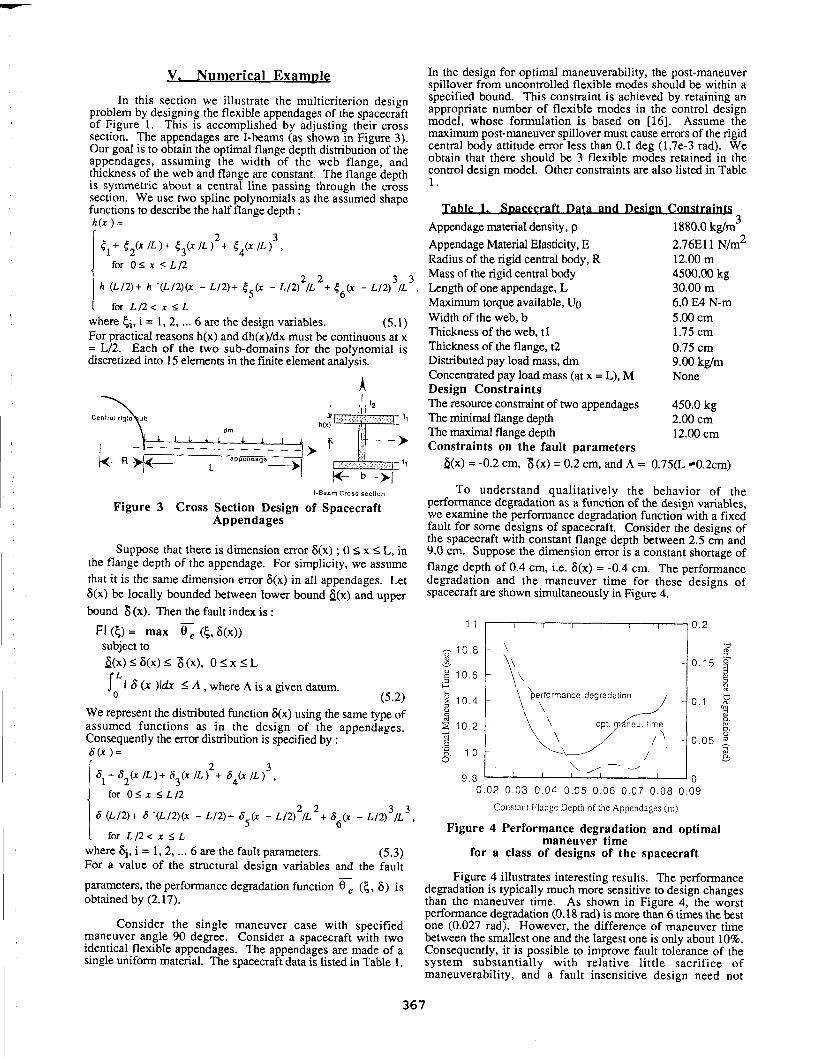
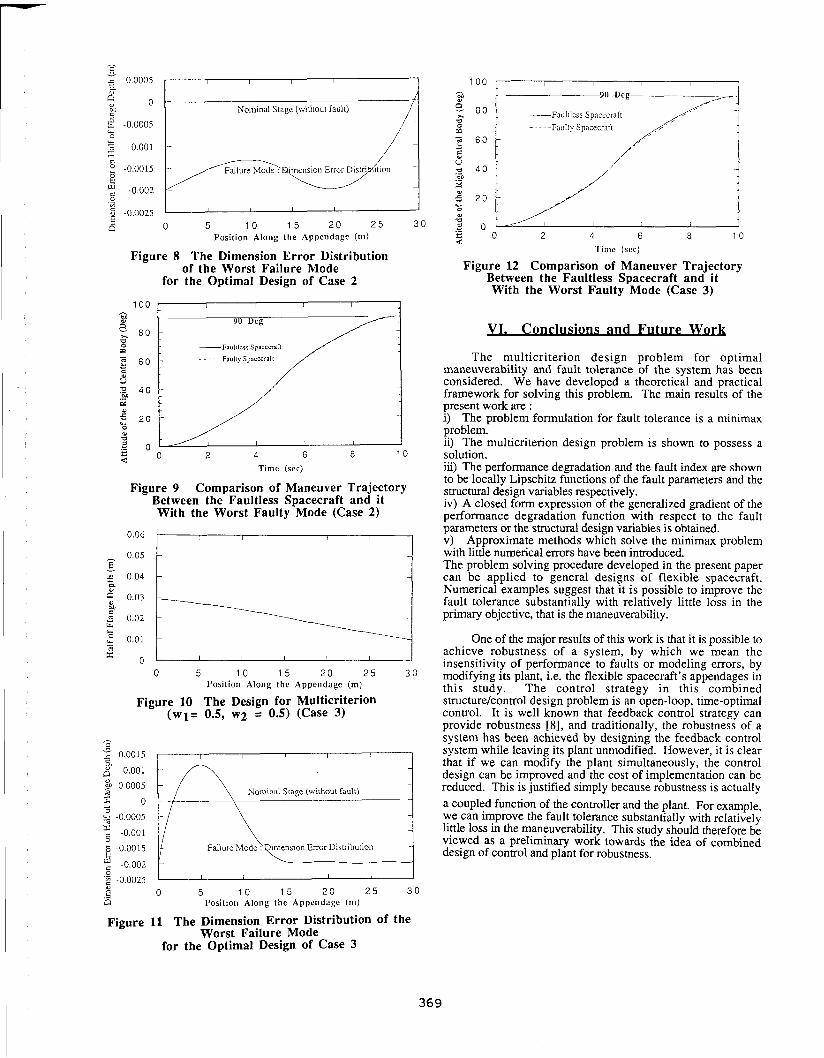
7.92497D-03, thus E~ = 5.075e-1 %. We accept this design as the solution for optimal fault tolerance. Therefore the fault index is EMk = 7.90757e-03 rad. The optimal maneuver time of this design is 9.924508 sec. The flange depth distribution of this design is shown in Figure 10, and the worst dimension error distribution is shown in Figure I I. Note that the design in Case 3 is very similiar to that in Case 2, both in optimal maneuver time and fault index. The comaprison of the maneuver trajectories between the faultless spacecraft and it with the worst faulty mode is shown in Figure 12.

To compare the results of these cases, we summarize them in Table 2.

9.91915 sec 2.60572e-02 rad (1.493 Deg)

2. Design of optimal fault tolerance (wl = O., w2 = 1.0) 9.92519 sec 7.90757e-03 rad (0.453 Deg)

3. Multicriterion design of the optimal maneuverability and fault tolerance (wl = 0.5, w2 = 0.5)

9.924508 sec 7.92497e-03 rad (0.454 Deg)

Table 2 Summary of results

It is observed from Table 2 that we can actually improve the fault tolerance substantially with relatively little sacrifice of the primary objective, the maneuverability. The fault index of Case 1 is about 3 times it of Case 3, while the difference of maneuver time between them is only 1 %.

O L 1 I I 1 I 0 5 1 0 1 5 .20 25 30

I'osition Along t h e Appendage (111)

Figure 5 The Design for Optimal Maneuverability (Case 1)

. - --= -9(bDc-7-7

----Fnuliless Sp:icccraft - - - Fauliy Spacecraft

-

/' Time (sec)

Figure 6 Comparison of Maneuver Trajectory Between the Faultless Spacecraft and it With the Worst Faulty Mode (Case 1)

Figure 7 The Design for Optimal Fault Tolerance (Case 2)

- 6 - + 0.0005 I I I I I

! 0 . M Nominal Stage (without fault) 9 E -0.0005 - (I

3 -0.001 -

5 -0.0015 -

6 t: : -0.002 0 .+ w

6 -0.0025 I I I I , E a o 5 1 0 1 5 2 0 2 5 3 0

Position Along the Appendage (111)

Figure 8 The Dimension Error Distribution of the Worst Failure Mode

for the Optimal Design of Case 2

Time (scc)

Figure 9 Comparison of Maneuver Trajectory Between the Faultless Spacecraft and it With the Worst Faulty Mode (Case 2)

0 5 1 0 1 5 2 0 2 5 3 0 Position Along the Appendage (m)

Figure 10 The Design for Multicriterion ( w l = 0.5, w2 = 0.5) (Case 3)

- Nominal Stage (without fault)

-

-

-

0 '" -0.0025 I I I I 1 I B .E 0 5 1 0 1 5 2 0 2 5 3 0 C1 Position Along the Appendage (111)

Figure 11 The Dimension Error Distribution of the Worst Failure Mode

for the Optimal Design of Case 3

-FwI[Icss Spacecraft

Faulty Spacecraft

Figure 12 Comparison of Maneuver Trajectory Between the Faultless Spacecraft and it With the Worst Faulty Mode (Case 3)

VI. Conclusions and Future Work

The multicriterion design problem for optimal maneuverability and fault tolerance of the system has been considered. We have developed a theoretical and practical framework for solving this problem. The main results of the present work are : i) The problem formulation for fault tolerance is a minimax problem. ii) The multicriterion design problem is shown to possess a solution. iii) The performance degradation and the fault index are shown to be locally Lipschitz functions of the fault parameters and the structural design variables respectively. iv) A closed form expression of the generalized gradient of the performance degradation function with respect to the fault parameters or the structural design variables is obtained. v) Approximate methods which solve the minimax problem with little numerical errors have been introduced. The problem solving procedure developed in the present paper can be applied to general designs of flexible spacecraft. Numerical examples suggest that it is possible to improve the fault tolerance substantially with relatively little loss in the primary objective, that is the maneuverability.

One of the major results of this work is that it is possible to achieve robustness of a system, by which we mean the insensitivity of performance to faults or modeling errors, by modifying its plant, i.e. the flexible spacecraft's appendages in this study. The control strategy in this combined structure/control design problem is an open-loop, time-optimal control. It is well known that feedback control strategy can provide robustness [8], and traditionally, the robustness of a system has been achieved by designing the feedback control system while leaving its plant unmodified. However, it is clear that if we can modify the plant simultaneously, the control design can be improved and the cost of implementation can be reduced. This is justified simply because robustness is actually a coupled function of the controller and the plant. For example, we can improve the fault tolerance substantially with relatively little loss in the maneuverability. This study should therefore be viewed as a preliminary work towards the idea of combined design of control and plant for robustness.

VI. References

J. Ling, P. Kabamba, and J. Taylor, "Combined Design of Structures and Controllers for Optimal Maneuverability," to appear on Structural Optimization.. R. M. Byers, S. R. Vadali, and J. L. Junkins, "Near- Minimum Time Close-Loop Slewing of Flexible Spacecraft," Journal of Guidance, Control, and Dynamics, Vol. 13, No. 1, pp. 57-65, Jan.-Feb. 1990. C. A. Mota Soares (ed.), Computer Aided Optimal Design : Structural and Mechanical Systems, NATO AS1 Series, Heidelberg, New York, 1987. P. F. Sun, J. S. Arora, and E. J. Haug, "Fail Safe Optimal Design of Structures," Journal of Engineering Optimization, pp. 45-53,Vol. 2, No. 1, 1976. R. T. Haftka, "Damage Tolerant Design using Collapse Techniques," AIAA Journal, pp. 1462-1466, Vol. 21, No. 10, 1983. J. E. Taylor and N. Kikuchi, "Optimal Fail-safe Design : A Multicriterion Formulation," Proc. 16th ICTAM Congress, Copenhagen, 1984. J. E. Taylor, and M. P. Bendsoe, "An Interpretation for Min-Max Structural Design Problems Including a Method for Relaxing Constraints," Int. J. Solids Structures, pp. 301-314, Vol. 20, NO. 4, 1984. J. Lunze, Robust Multivariable Feedback Control, Prentice Hall Int'l, 1988. J. W. Howze and R. K. Cavin, "Regulator Design with Modal Insensitivity," lEEE TAC - 24, pp. 466-469, No. 3, 1979. K. B. Lim, and J. L. Junkins," Minimum Sensitivity Eignevalue Placement via Sequential Linear Programming, Proceedings of the Mountain Lake Dynamics and Control Institute, edited by J. L. Jukins, 1985. J. R. Newsom and V. Mukhopadhyay, "A Multiloop Robust Controller Design Study Using Singular Value Gradients," Journal of Guidance, Control, and Dynamics, pp. 514-519, Vol. 8, NO. 4, 1985. R. L. Kosut, H. Salzwedel, and A. E. Naeini, "Robust Control of Flexible Spacecraft," Journal of Guidance, Control, and Dynamics, pp. 104-1 11, Vol. 6, 1983. K. B. Lim and J. L. Junkins, "Robustness Optimization of Structural and Controller Parameters," Journal of Guidance, Control, and Dynamics, pp. 89-96, Vol. 12, No. 1, 1989. S. Rao, T.-S. Pan, and V. B. Venkayya, "Robustness Improvement of Actively Controlled Structures through

Structural Modification," AIAA Journal, pp. 353-361. -.

February, 1990. L. H. Keel, K. B. Lim and J.-N. Juang,"Robust Eigenvalue Assignment with Maximum Tolerance tn - ~ G t e m ~ncertain%es," Journal of Guidance, Control, and Dynamics, pp. 615-620, 1991. G. Singh, P. T. Kabamba, and N. H. McClamroch, "Planar, Time-Optimal, Rest-to-Rest Slewing Maneuvers of Flexible Spacecraft," Journal of Guidance, Control, and Dynamics, Vol. 12, No. 1, pp. 71-81, 1989. D. S. Bernstein, and W. M. Haddad, "Robust Stability and Performance Analysis for State Space Systems via Quadratic Lyapunov Bounds, " SIAM J. Matrix Anal. Appl., Vol 11, No. 12, pp. 239 - 271, April, 1990. IS. Zhou and P. P. Khargonekar, "Stability Robustness Bounds for State-Space Models with Structured Uncertainty," IEEE TAC - 32, No. 7, pp. 621 - 623, 1988. F. H. Clarke, Optimization and Nonsmooth Analysis, Wiley-Interscience, Canada, 1983. C. Lemarechal and R. Mifflin (ed.), Nonsmooth Optimization, Pergamon Press, New York, 1978. C. Lemarechal, "Method of Descent for Nondifferentiable Optimization," SIAM Review, March, 1988. D. M. Salmon, "Minimax Controller Design," IEEE TAC - 13, NO. 4, pp. 369 - 376, 1968. A. Osyczka (ed.), Multicriteria Design Optimization, Procedures and Applications, Heidelberg, New York, 1990. J. Ling, P. Kabamba, and J. Taylor, "Multicriterion Structure/Control Design for Optimal Maneuverability and Fault Tolerance of Flexible Spacecraft," to appear on Jowml of Optimization Theory and Application.