Embed Size (px)
Citation preview

MULTI-OBJECTIVE OPTIMIZATION FOR SPEED
AND STABILITY OF A SONY AIBO GAIT
THESIS
Christopher A. Patterson, Second Lieutenant, USAF
AFIT/GCS/ENG/07-17
DEPARTMENT OF THE AIR FORCE AIR UNIVERSITY
AIR FORCE INSTITUTE OF TECHNOLOGY
Wright-Patterson Air Force Base, Ohio
APPROVED FOR PUBLIC RELEASE; DISTRIBUTION UNLIMITED

The views expressed in this thesis are those of the author and do not reflect the official policy or position of the United States Air Force, Department of Defense, or the United States Government.

AFIT/GCS/ENG/07-17
MULTI-OBJECTIVE OPTIMIZATION FOR SPEED AND STABILITY OF A SONY AIBO GAIT
THESIS
Presented to the Faculty
Department of Electrical and Computer Engineering
Graduate School of Engineering and Management
Air Force Institute of Technology
Air University
Air Education and Training Command
In Partial Fulfillment of the Requirements for the
Degree of Master of Science in Computer Science
Christopher A. Patterson, BS
Second Lieutenant, USAF
September 2007
APPROVED FOR PUBLIC RELEASE; DISTRIBUTION UNLIMITED.

AFIT/GCS/ENG/07-17 MULTI-OBJECTIVE OPTIMIZATION FOR SPEED AND STABILITY OF A SONY
AIBO GAIT
Christopher A. Patterson, BS Second Lieutenant, USAF
Approved: /signed/ 31 Aug 07
_________________________________ Dr. Gilbert L. Peterson (Chairman) date
/signed/ 31 Aug 07
_________________________________ Dr. Gary B. Lamont (Member) date
/signed/ 31 Aug 07
_________________________________ Maj Christopher B. Mayer (Member) date

AFIT/GCE/ENG/07-17
Abstract
Locomotion is a fundamental facet of mobile robotics that many higher level
aspects rely on. However, this is not a simple problem for legged robots with many
degrees of freedom. For this reason, machine learning techniques have been applied to
the domain. Although impressive results have been achieved, there remains a
fundamental problem with using most machine learning methods. The learning
algorithms usually require a large dataset which is prohibitively hard to collect on an
actual robot. Further, learning in simulation has had limited success transitioning to the
real world. Also, many learning algorithms optimize for a single fitness function,
neglecting many of the effects on other parts of the system.
As part of the RoboCup 4-legged league, many researchers have worked on
increasing the walking/gait speed of Sony AIBO robots. Recently, the effort shifted from
developing a quick gait, to developing a gait that also provides a stable sensing platform.
However, to date, optimization of both velocity and camera stability has only occurred
using a single fitness function that incorporates the two objectives with a weighting that
defines the desired tradeoff between them. However, the true nature of this tradeoff is not
understood because the pareto front has never been charted, so this a priori decision is
uninformed. This project applies the Nondominated Sorting Genetic Algorithm-II
(NSGA-II) to find a pareto set of fast, stable gait parameters. This allows a user to select
the best tradeoff between balance and speed for a given application. Three fitness
functions are defined: one speed measure and two stability measures. A plot of evolved
gaits shows a pareto front that indicates speed and stability are indeed conflicting goals.
Interestingly, the results also show that tradeoffs also exist between different measures of
stability.
iv

Acknowledgements
This document represents a year of my life, but it would not have been possible
without the help of others. I’d like to extend my most sincere thanks to Dustin, Melanie,
Adrian, Adam, Dan, and Erik for helping me program, write and format. My appreciation
also goes to Bronwyn, Ginny, Michelle, Mary Ashley, and Heather for always lending
me an ear and helping me regain my focus. Finally, I owe a great deal to my family,
teachers, and advisor for their support and sacrifices that have gotten me to this point.
v

Contents
Page
Abstract ...................................................................................................................... iv
Acknowledgements.................................................................................................... v
List of Figures ............................................................................................................ ix
List of Tables ............................................................................................................. x
List of Abbreviations ................................................................................................. xi
1 Introduction.................................................................................................... 1
1.1 Objectives .......................................................................................... 3
1.2 Outline................................................................................................ 4
2 Related Work ................................................................................................. 5
2.1 Gait Parameterization......................................................................... 6
2.1.1 Body Centered Gait Parameterization ............................. 6
2.1.2 Foot Based Gait Parameterization ................................... 7
2.2 Gait Learning ..................................................................................... 9
2.2.1 Reinforcement Learning .................................................. 10
2.2.2 Powell’s Method .............................................................. 11
2.2.3 Evolutionary Algorithms ................................................. 11
2.2.4 Comparing Learning Techniques..................................... 14
2.3 Learning with Multiple Objectives .................................................... 15
2.4 Multi-Objective Evolutionary Algorithms......................................... 17
2.5 Summary ............................................................................................ 22
3 Methodology.................................................................................................. 23
vi
3.1 Gait Representation............................................................................ 23
3.2 Gait Parameterization......................................................................... 24
3.3 Fitness Evaluation.............................................................................. 25
3.3.1 Speed................................................................................ 25
3.3.2 Jitter.................................................................................. 26
3.3.3 Tilt.................................................................................... 27
3.4 Nondominated Sorting Genetic Algorithm-II.................................... 27
3.4.1 Genetic Algorithm Design ............................................... 27
3.4.2 Fitness Function Integration ............................................ 29
3.5 OPEN-R Software.............................................................................. 30
3.5.1 Architecture and Control Flow Design ............................ 30
3.5.2 Parameter Translation ...................................................... 32
3.5.3 Color Detection................................................................ 34
3.5.4 Fitness Function Automation........................................... 35
3.6 Summary ............................................................................................ 37
4. Experimental Results ..................................................................................... 38
4.1 Experimental Setup............................................................................ 38
4.2 Gait Parameter Refinement................................................................ 40
4.3 Experiment Configurations................................................................ 44
4.4 Quantitative Results ........................................................................... 46
4.4.1 Effect of GA Parameter Tuning....................................... 46
4.4.2 Nature of Trade-Off Between Fitness Functions ............. 49
4.5 Empirical Observations...................................................................... 54
vii
4.5.1 Effects on the Robot......................................................... 54
4.5.2 Effects of Learning .......................................................... 55
4.5.3 Effects on Fitness Scores ................................................. 56
4.6 Summary ............................................................................................ 58
5. Conclusions and Future Work ....................................................................... 59
5.1 Future Work ....................................................................................... 59
5.1.1 Fitness Function Revision................................................ 60
5.1.2 Optimization Method....................................................... 62
5.1.3 Automation ...................................................................... 62
5.1.4 Head Stabilization............................................................ 63
5.3 Conclusions........................................................................................ 63
Appendix A. Data for Figure 4.5............................................................................. 65
Appendix B. Data for Figure 4.7............................................................................. 66
Bibliography .............................................................................................................. 67
viii

List of Figures
Figure Page
3.1 Example of Walk Locus (Adapted from [42]) ................................... 24
3.2 Breakup of Locus into 18 Points Specified by 25th
Parameter of 9 .......................................................................................... 25
3.3 Experimental Environment ................................................................ 26
3.4 Software Architecture with Message Passing.................................... 32
4.1 Naming Convention of Gait Parameters (Adapted from [24]) .......... 40
4.2 Time Progression, Run 8.................................................................... 47
4.3 Time Progression, Run 9.................................................................... 48
4.4 Time Progression, Run 10.................................................................. 48
4.5 Time-Jitter Tradeoff, Run 8 ............................................................... 49
4.6 Time-Jitter Tradeoff, Runs 8, 9, & 10 ............................................... 50
4.7 Jitter-Tilt Tradeoff, Run 10................................................................ 51
4.8 Time-Jitter Tradeoff, Runs 8, 9, & 10 ............................................... 51
4.9 Time-Tilt Tradeoff, Run 8 ................................................................. 52
4.10 Time-Tilt Tradeoff, Run 9 ................................................................. 53
4.11 Time-Tilt Tradeoff, Run 10 ............................................................... 53
5.1 Offset Causes: A. Body Twist, B. Body Alignment .......................... 61
ix

List of Tables
Table Page
4.1 Evolution of Parameter Ranges ......................................................... 43
4.2 Initial Generic Algorithm Parameters................................................ 44
4.3 Final Experiment Parameters............................................................. 46
4.4 Best Scores Runs 8-10 ....................................................................... 47
A.1 Non-Dominated Points (Based on Time-Jitter projection), Run 8 .... 65
B.1 Non-Dominated Points (Based o Jitter-Tilt projection), Run 10 ....... 66
x

xi
List of Abbreviations
Abbreviation Page
NSGA-II Nondominated Sorting Genetic Algorithm-II.................................... xi
ASIC application-specific integrated circuit................................................ 6
ERS Entertainment Robot System ............................................................. 6
UNSW University of New South Wales ........................................................ 8
UT University of Texas............................................................................ 8
EA evolutionary algorithm....................................................................... 11
GA genetic algorithm ............................................................................... 12
MOEA multi-objective evolutionary algorithm ............................................. 19
GENMOP general multi-objective parallel ......................................................... 20
QCL quantum cascade laser........................................................................ 20
MOP multi-objective problem..................................................................... 21
ONVG Overall Non-Dominated Vector Generation...................................... 21
CDT Color Detection Table........................................................................ 34
SDK Software Development Kit ................................................................ 34

MULTI-OBJECTIVE OPTIMIZATION FOR SPEED AND STABILITY OF A SONY
AIBO GAIT
1. Introduction
One of the driving forces in robotics research is the RoboCup competition. This is
an annual, international competition in which robotic soccer teams compete against each
other. The stated goal of the RoboCup organization is to “develop a team of fully
autonomous humanoid robots that can win against the human world soccer champion
team” by 2050 [33]. The RoboCup competition provides an environment where
competition drives research which is then applied to a real world situation. To compete in
a RoboCup tournament, teams must solve many of robotics’ core problems. For example,
they must develop locomotion modules that allow the robot not only to move, but also
manipulate the ball. They must be able to localize their position and navigate around the
field. Vision is also important as colors, objects, teammates, and opponents need to be
recognized. Further, not only must the robots make and execute a plan for themselves,
but inter-agent cooperation is possible. In addition to the soccer tournament itself,
RoboCup poses other challenges to push the envelope of robotic technology. Usually
these challenges relate to the soccer domain, such as testing robots’ ability to complete
passes and recognize and score on different types of goals.
There are several RoboCup leagues that use simulated, wheeled, and legged
robots. One of these is the four-legged league, which uses Sony AIBO robots [33].
Legged robots have an advantage over wheeled robots in that they contact the ground at
distinct points versus the continuous path of wheeled robots. This makes them able to
1

move over rougher terrain than wheeled robots. They also have the advantage of being
able to strafe sideways and step over obstacles, such as trip wires. On the other hand,
wheeled robots can achieve greater speed on even terrain, so legged robot gaits are
designed to mimic wheel motion. Additionally, designing a gait controller is a difficult
problem when attempted by hand [9] and is only a small part of the challenge to deploy a
fully autonomous robot in an unstructured, dynamic environment [22]. Part of the
difficulty in creating a gait controller is that the problem does not fit the commonly
applied divide-and-conquer software development strategy. How to decompose a
controller, is not obvious, interactions are not limited to direct connecting links, and
interactions between sub-parts grow exponentially as joint complexity increases [38].
Despite the difficulty, trends have emerged in legged robotics study. Research on
legged robots has focused on hexapod, quadruped, and biped robots [1] [6] [25]. Machine
learning techniques have also been applied to the domain of gait development. For
example, the locomotion control problem has been addressed using evolutionary
algorithms to find neural network controllers [1] [21] [29], dynamically-rearranging
neural network controllers [6] [25], and central pattern generators [30] [31]. Another
trend is to use simulation as the primary method for research. Learning conducted in
simulation has been shown in some instances to be portable to the real world [38].
However, simulation often transfers poorly to real environments which are too
complicated to simulate (e.g. modeling the fluid dynamics for an underwater robot) [14].
One trend that has unfortunately emerged is that when using an optimization
technique, only a single-objective function is used. This neglects many of the
interdependencies among the various aspects of robotic controllers. Using the RoboCup
2

example, movement affects locomotion, ball control, and vision. However, most
movement research has sought only to increase speed, thus improving locomotion while
neglecting ball control and vision.
The alternate approach, as presented here, is to use a multi-objective optimization
technique, such as a multi-objective genetic algorithm. A multi-objective genetic
algorithm is a stochastic search technique inspired by biological concepts. In particular, a
population of solutions is evolved such that scores improve along multiple objective
functions. The multi-objective genetic algorithm produces a variety of solutions that can
represent tradeoffs between the multiple objectives, and, during operation, can be
switched between as priorities change. For example, a fast gait that neglects ball control
can be selected when the robot does not have possession of the ball, which is then
switched with a gait that sacrifices some speed for ball control once the robot gets the
ball. In terms of a gait, ball control is improved with a more stable walk that allows for
better navigation and object tracking and identification.
1.1 Objectives
This project fills one of the voids left by a focus on single-objective optimization.
Using the standard robot for the RoboCup quadruped league, a multi-objective genetic
algorithm is applied to study the tradeoff between movement speed and camera stability.
Camera stability is a critical factor in object classification and has effects that spill over
to localization and planning [34]. Previously, these effects have been sorely neglected as
leg movement has been optimized only for speed. In order to accomplish this task, the
following objectives are established:
- Develop a parameterized walk method
3

- Develop a way to score different walks for both speed and stability
- Use a multi-objective genetic algorithm to develop fast, stable gaits
- Analyze the results of the genetic algorithm to better understand the
speed-stability tradeoff
1.2 Outline
The rest of this document is organized as follows: Chapter II discusses other work
related to the development of gaits for the AIBO. This is followed by the method used to
characterize the speed/stability tradeoff. Section IV reports results, showing a clear
tradeoff between speed and stability as well as between different stability characteristics.
The thesis concludes with a discussion of the potential application of this research and an
outline for future work.
4

2. Related Work
A survey of behavior development for evolutionary robotics shows that previous
research focuses mainly on generating behaviors satisfying a single-objective function.
Further, when multiple fitness-functions are used, they are often aggregated together to
form a single, weighted objective function[38]. A multi-objective approach is superior
because it generates multiple, non-dominated solutions in a single run, minimizing
experimental effort. Additionally, the aggregation of multiple objectives into a single
objective requires assumptions about the fitness score ranges and nature of the pareto
front.
One example of where single-objective fitness functions have dominated research
areas is the learning of a gait on the Sony AIBO. The AIBO is a quadruped robot that is
used in the four-legged RoboCup league. Because it is used in this annual competition,
research effort has focused on several methods to develop a fast walk for this particular
robot. This research is concentrated in two areas, the parameterization of the gait and the
machine learning techniques used. Although many machine learning techniques have
been applied to this problem, and multi-objective optimization techniques have been
applied to develop other behaviors, this is the first use of a multi-objective genetic
algorithm to tune AIBO gait parameters.
The remainder of this chapter provides an overview of the previous research that
is necessary in completing the objectives of this project. First, Section 2.1 outlines the
various ways that others have parameterized a quadruped gait. Next, machine learning
methods that have been applied to this problem are discussed. The final two sections
5

cover multi-objective optimization methods and, specifically, multi-objective
evolutionary algorithms.
2.1 Gait Parameterization
At the lowest level, AIBO gaits are determined by a series of angles for each of
the twelve leg joints. These angles are input to an application-specific integrated circuit
(ASIC) chip, which controls the servos in the legs. A potentiometer is used to sense the
current joint angles and the ASIC chip determines the motor inputs necessary to achieve
the target angles. This cycle occurs every eight milliseconds. A higher level approach is
to define several parameters to characterize a gait. A software program, or locomotion
engine, converts these parameters into a series of target angles which are fed to the ASIC
chip.
Optimization of these parameters, or gait optimization becomes a search through
the parameter space for the locomotion engine. Researchers have used several different
parameterizations to define gaits on the AIBO. These parameterizations can be divided
into two types: those that are focused on the movement of the body in relationship to the
ground [3] [14] and those that are focused on the movement of the feet in reference to the
body [11] [23] [28].
2.1.1 Body Centered Gait Parameterization In developing the gait for the first
commercially available AIBO (ERS-110), Sony scientists used a body centered
parameterization, the majority of which specified the position and orientation of the body,
as well as the body’s oscillation through the cyclical walking cycle. Other parameters
also described the timing of the gait, such as its period and the phasing of each leg. In
total, twenty-one parameters were used to describe the gait. On a second experiment they
6

also parameterized the phases of the legs. With this method Hornby, et al. were able to
develop both a trot and a pace gait and achieve a maximum speed of 600 cm/min [14].
However, they concluded that a gait developed in one environment would work in an
easier environment but not necessarily in a harder environment. Thus, they constructed a
“hard” environment to train in and produced a robust gait. This process proved to be very
heavily impacted by the learning environment and platform, and did not prove to be
applicable in extremely unpredictable environments [14]. In subsequent experiments
meant to address these problems, the authors developing a gait that moved at 900 cm/min
[15].
In another example of a body centric parameterization, researchers from Carnegie
Mellon University make use of an acceleration model to describe the trajectory of the
body and time offsets to determine the phasing of the legs [3]. While a leg is on the
ground, it is moved in compliance with this trajectory. Once it is lifted, a target location
for it to be set down is generated and it moves towards its target. The Carnegie Mellon
team used this twelve-variable parameterization to learn gaits for the Sony AIBO (ERS-
210) that achieved a maximum speed of 290±6 mm/sec (1740 cm/min). However, in both
of the two best gaits developed with this method, the knees and elbows collide. While
this did not seem to harm the robot, the possibility exists that it may define a walk where
such collisions pose a threat to the robot.
2.1.2 Foot Based Gait Parameterization Foot based parameterizations define a
gait by describing a shape or locus, in relation to the body, for the feet to travel around.
These loci are divided into a set of points based on the frequency of the gait, and inverse
kinematics is used to determine the next set of target joint angles. This method keeps
7

each pair of diagonal legs in phase with each other and perfectly out of phase with the
other pair. By using symmetry between the left and right sides, it nearly eliminates the
problems of turning and falling over. Defining a gait in this way also constrains the
search space to reduce wear on the robot. Additionally, the loci can be rotated enabling
turning, strafing, and backing up.
This method was first introduced in [11] where the authors proposed a rectangular
locus for use on the AIBO ERS-110. This method resulted in a walk that achieved a
speed of 1200 cm/min, an improvement over fastest gait at the time of 900 cm/min
reported in [15]. While this method suffered interference from the robot’s claws, it gave
the University of New South Wales (UNSW) team a distinct advantage over the other
teams and has spawned investigation into other locus based gaits.
In order to solve the problem of the robot’s claws catching and dragging, the
UNSW team transitioned from a rectangular to a quadrilateral. They described two
quadrilaterals, one for the front legs and one for the hind legs, using the corners of each
quadrilateral. This results in eight points in three dimensional space or twenty-four
parameters. However, instead of representing the points based on a coordinate system,
they represented the points using twenty four stretches and translations, thus capturing
key interrelations among the points. Using this method produced a gait that walked at
26.99±0.50 cm/sec (1619 cm/min) on the ERS-210A. However, the inverse kinematics
failed to ensure the front feet were below the elbows, so the robot used its forearms as
skis, resulting in less of a walk and more of a crawl. [18]
Another example of a locus based gait parameterization is the one used by the
University of Texas (UT) at Austin team [23]. In this approach, the loci is characterized
8

as two half ellipses, one for the front and one for the hind legs. This technique uses a total
of twelve parameters, including one that controlled the fraction of time each foot spends
on the ground, also called its duty time. Despite this parameter, the half ellipse method
implements a trot gait by keeping each pair of diagonal legs synchronized. While this
parameterization proved effective in generating a walk with speed 291±3 mm/sec (1746
cm/min) on the ERS-210A, the path of the robot’s feet did not actually follow an ellipse
as predicted. The first reason for this is because the best gait set the duty parameter below
0.5. Thus, the feet were on the ground part of the time the parameterization meant for
them to be in the air. Another reason that the actual locus was different than expected was
because the authors used the axis of the ellipse to determine the path of the foot while it
was on the ground.
A fourth locus shape was implemented by researchers at the University of
Newcastle [28]. They implemented an arbitrarily shaped locus on the ERS-201A using
straight lines to connect a series of ten points. For comparison, they also implemented a
rectangular, ellipsoid, and trapezoidal locus. They found that the trapezoidal locus was
fastest, ellipsoid second, and the rectangular last. The arbitrarily shaped locus, however,
proved faster than any of the other shapes with a reported speed of 29.65±0.7 cm/sec
(1770 cm/min). While this resulted in only a modest speedup over previous methods, it
could only be achieved by greatly expanding the parameter space.
2.2 Gait Learning
Once a gait has been parameterized, the parameters must be tuned in order to
produce a walk with the desired behavior. Tuning these parameters can be a long,
complex, and tedious task. However, by defining a fitness function, tuning the parameters
9

becomes a multi-dimensional optimization problem, for which many automated methods
exist. Another advantage of automating this process is that it eliminates human bias. Gait
parameter optimization has, in fact, been the subject of much research, and generally
results in better gaits than hand tuning.
2.2.1 Reinforcement Learning The UT Austin team implemented a policy
gradient reinforcement learning method to tune the half ellipse locus in [23]. Use of this
method assumes that the fitness function is differentiable. However, because the
functional form of the problem space is unknown, the gradients must be estimated. They
did this by generating a number of random permutations of the parameters. This was
done by taking each component of the current parameter set and either adding or
subtracting a fixed amount or not changing the component. These sets were evaluated on
the robot and used to form estimates of the partial derivative for each component. Based
on the best scores, the parameter set was changed and the cycle continued. The fitness
function, defined as the time it took the AIBO to walk between two fixed landmarks, was
set to be minimized. Because of the noise in the AIBOs’ sensors, each evaluation was
completed three times and averaged. The learning took place on a desktop computer
which delegated the evaluation of each parameter set to one of three AIBO ERS-210As.
The only human intervention required in this process was to replace batteries. This
method generated a gait that moved at 291 mm/sec (1746 cm/min), an improvement from
their best hand tuned speed of 245 mm/sec (1470 cm/min). One advantage of this method
is that it can be distributed over many AIBOs, decreasing the time needed for learning.
However, it required moderately hand tuned parameters in order to find its fastest gait.
10

This means that not only is the method prone to hone in on local optima, but also that it
cannot be used to find an initial gait.
2.2.2 Powell’s Method The UNSW team has also automated its parameter
tuning as reported in [18]. Like the UT Austin team, it had the robot walk between two
fixed points and had time minimization as the fitness function. They implement Powell’s
direction set method. This method uses the initial parameters as directions and modifies
each direction in turn, finding its minimum value and then moving on to the next
direction. Once it has completed all directions, it uses knowledge gained from the current
iteration to determine a new set of directions for the next iteration. However, this method,
when employed by UNSW, failed to meet the goal of reducing the time necessary for
training to a reasonable period. Indeed, the algorithm did not have the opportunity to run
to completion because the processing time exceeded constraints. Another flaw is that this
method also assumes that the sample space is differentiable. The end result was a gait that
enabled the ERS-210A to move at 26.99±0.50 cm/sec (1619 cm/min) compared to the
hand tuned gait that had a speed of 25.42±0.50 cm/sec (1525 cm/min). Finally, the
optimization technique got stuck in a local minimum and needed to be rolled back to a
previous state in order to continue finding improvement.
2.2.3 Evolutionary Algorithms One of the more popular optimization
techniques is to use an evolutionary algorithm (EA). EAs work on several solutions at
once, called a population. During an iteration, each solution, or individual, in the
population is evaluated using the fitness function, and then evolutionary operators are
applied. These operators are inspired by biology and include techniques such as
recombination, crossover, and mutation. EAs have many advantages over other
11

optimization methods. For example, they do not rely on any characteristics of the search
space. Another advantage comes from the fact that most of the computational cost of an
optimization problem lies in evaluating the fitness function. Since EAs operate on a
population of individuals, the fitness function calculations can be easily parallelized.
These advantages have led to EAs being used as the method of choice for AIBO gait
optimization.
In fact, the gait that shipped with the first commercially available AIBO was
configured using an evolutionary algorithm. The development of this gait is documented
in [14]. The evolutionary algorithm began with randomly generated gaits that were first
tested to make sure they did not cause the robot to fall. As a fitness function, distance
traveled in a given timeframe and the straightness of the walk is multiplied together.
These values were attained using the robot’s onboard sensors. This process also
compensated well to noise in the problem space. To do this, the authors averaged sensor
readings and implemented an age in the evolutionary algorithm that forced periodic
recalculation of the fitness function. This method proved successful on both the OPEN-R
Prototype and ERS-110 AIBOs. The walk approved for release with the ERS-110 moved
at 900 cm/min, faster than the fastest hand-tuned gait of 660 cm/min [15].
The Carnegie Mellon team also employed a genetic algorithm because of its high
convergence rate, ability to find optima independent of initial parameters, resistance to
noise, and parallelizability. A genetic algorithm (GA) is one flavor of evolutionary
algorithms. In order to compensate for the problem of local optima, the team introduced a
concept of radiation to force mutation if too many individual solutions became tightly
grouped. The learning process consisted of two phases. The first phase explored a large
12
solution space, while the second took what was learned from the first phase and fine-
tuned the solution. In order to deal with noise, solutions with a high fitness level were
double checked by recalculating the fitness and averaging the two results. Additionally,
all individuals are reevaluated every ten to fifteen generations. Distance traveled was the
only measure of fitness, which was evaluated on the robots. The robots first used
kinematics to ensure the gait poses no threat to their hardware and then executed it, using
their onboard sensors to determine distance traveled. The only human interaction required
was to change the batteries. The genetic algorithm, on the other hand, ran on an external
computer. The robots and computer communicated using a wireless network. This
architecture allowed the authors to parallelize the fitness calculations. They were able to
evolve a gait for the ERS-210 that moved at 290±6 mm/sec (1740 cm/min), an
improvement over the hand-tuned walk speed of 235 mm/sec (1410 cm/min) [3].
Another example of evolutionary gait learning is presented by Quinlin, et al. [28].
In this instance, the authors used an Evolutionary Hill Climbing with Line Search
algorithm. This algorithm was chosen for its quick learning rate. Again the fitness
function was time. The ERS-210A robots ran 190 cm, using their vision system to stop
each run, and used camera frames as a measure of time. Each traversal was completed
twice for a single episode. This algorithm was first run on rectangular, ellipsoid, and
trapezoidal trajectories and improved on the best parameter set for all three. It was then
run on the arbitrary locus shape and resulted in a gait with speed of 29.65±0.7 cm/sec
(1779 cm/min). However, the technique was only able to fine-tune the parameters
initially set in a working fashion. One final insight from this method was that many
different solutions yielded similar results.
13
2.2.4 Comparing Learning Techniques Kohl and Stone [22], note that gait
optimization poses two challenges over other multi-dimensional optimization problems.
First, large amounts of data are prohibitively difficult to collect because of maintenance
required on the robots and constant human supervision. This requires the optimization
algorithm be effective with small amounts of data. Second, the dynamic complexity of
many robots means they cannot be faithfully simulated and even when possible, using
simulation lessens the unstructured and unpredictable nature of a real world environment
[22]. Thus, researchers must test and compare different algorithms to see which is most
effective. The four algorithms used by Kohl and Stone are hill climbing, amoeba, genetic,
and policy gradient. Note that the Policy Gradient algorithm is the same as in their
previous work [23]. Each gait is tested on the AIBOs while the learning occurs on a
central computer. Because of the noise in the AIBOs’ sensors, each evaluation is
completed three times and averaged. They compare the results of each algorithm by
comparing the velocity of the resulting gaits, as well as the sample space that is explored
through the algorithm. Finally, they use a simulation to test how the algorithm degrades
when noise is introduced into the system.
While all four algorithms improved over hand tuned gaits, the hill climbing and
policy gradient algorithms were more successful than the other two. The authors
concluded that this was due to low coverage of the solution space by the amoeba and
genetic algorithms. Their attempts to correct this resulted in amoeba becoming
comparable to the other two algorithms and the genetic algorithm also slightly improved.
The amoeba algorithm also proved more susceptible to noise in the simulation. While the
14

policy gradient algorithm yielded the best results, it appears that all four algorithms are
comparable with the correct tuning.
2.3 Learning with Multiple Objectives
As gait speeds have increased, they have also become less steady. This leads to
unsteady camera images which in turn complicate vision-based behaviors such as ball
tracking and localization. Researchers from the University of Essex were the first to
address this issue [9]. They defined four fitness functions, forward/backward speed,
rotational speed, sideways speed, and stability. The speeds were obtained using an
overhead camera and the stability was measured using the onboard gyroscopes. The
authors performed a weighted sum of the four fitness functions and used a single-
objective genetic algorithm. For their GA they implemented roulette-wheel selection and
selection of the fittest. They used four recombination techniques in parallel: guaranteed-
uniform-crossover, guaranteed-average, guaranteed-big-creep, and guaranteed-little-
creep. They then applied mutation with a small probability. Finally, the probability of
each type of crossover was dependant on its success at generating good solutions in the
previous repetition.
The primary contribution of this effort was automating the parameter tuning
required for a genetic algorithm, which not only required less human interaction but also
made it more likely to evolve a good solution. From observing how the GA’s parameters
changed over time, they concluded that recombination was more effective in early
generations while mutation was more effective in later generations. However, they only
ran each solution once on the robots and used the onboard gyroscopes, both of which
introduced a lot of noise into the fitness function. Also, they used an overhead camera to
15
determine the distance traveled instead of using sensors onboard the robot. While it
would be easy to get information from the robot forward/backward motion, it is less
obvious how to use onboard sensors to evaluate the success of sideways and rotational
motion. Thus, it is unclear if this technique could be executed completely on a fielded
robot. Nonetheless, this experiment began to explore the tradeoffs between speed and
stability. The authors noted that stability quickly increased in the beginning and then
plateaued, until it decreased slightly at the end to allow a large speed increase.
In [34], the UT Austin team incorporates a concept of stability into their previous
work [22] [23], which uses a half ellipse foot path parameterization and policy gradient
optimization. The first technique the researchers employed was changing the fitness
function to account for both speed and stability. They weighted and minimize four
functions: time to walk a set distance, the standard deviation of the onboard
accelerometers, the distance a landmark was from the center of an image, and the angle
of the landmark in the image (it should have appeared vertically). The second technique
they employed was adding four parameters that moved the head in a cyclical ellipse. Here
the idea was that the image displacement caused by an unstable walk would be corrected
by moving the head. This, however, failed as the addition of head movement resulted in a
slower walk. This was either due to the head movement actually exacerbating the
problem or the added complexity rendering the optimization less effective. By factoring
in stability to their fitness function, the learned gait’s speed decreased from 340 mm/sec
(2040 cm/min) to 259 mm/s (1554 cm/min) on the ERS-7 but resulted in better object
classification (both increased true positives and decreased false positives). This
improvement in object classification is of the utmost importance, both in RoboCup and
16
other applications, because many higher level tasks require accurate object classification.
For example, localization is based on the identification of the field beacons and goals.
Also, play is heavily dependant on recognition of the ball and other robots. Certainly, the
gait has an impact on object recognition, and, in turn, most other aspects of the RoboCup
domain. Having established the importance of this interconnection, it clearly needs to be
understood further.
2.4 Multi-Objective Evolutionary Algorithms
The competing goals of both speed and stability have created an opportunity for
multi-objective optimization. While multi-objective optimization is an active field of
study, including the development of autonomous behaviors [10] [16] [7], the methods
have not yet been applied to AIBO gait development. For example, Teo and Abbass use
artificial neural networks to control a simulated quadruped robot. Using the Pareto-
frontier Differential Evolution algorithm, they balance the objectives of maximizing
speed and minimizing the size of the neural network [10]. Central Pattern Generators that
control a humanoid robot are also optimized using a GA. Here, the fitness functions are
designed to maintain balance, keep the robot upright, and maximize step length [16]. In
another case, a humanoid gait is evolved using the Strength Pareto Evolutionary
Algorithm to minimize the consumed energy and torque change [2]. Finally, a multi-
objective genetic program evolves controllers for a simulated unmanned aerial vehicle in
[7]. These fitness functions minimize the distance to target, maximize the amount of time
in level flight, and minimize the number of sharp, sudden turns.
The presence of multiple objectives in a problem leads to the existence of a set of
optimal solutions as opposed to a single solution. Without any further information, such
17

as the relative importance of each objective, it is impossible to say one solution in this set
is more desirable than another. Thus, in order to well define the optimized solution space,
many non-dominated solutions, or the pareto front, must be found. For terminology, a
solution A is said to be dominated if there exists another solution B such that B receives a
higher fitness score for all of the objectives. One method of doing this is to find one
solution at a time using a single-objective genetic algorithm and specifying different
objective tradeoffs. Obviously, this is overly burdensome and unpractical. Instead, a
number of multi-objective evolutionary algorithms have been suggested, which maintain
a set of non-dominated solutions which are reproduced and mutated in the search for a
pareto front.
One such algorithm is the non-dominated sorting genetic algorithm or NSGA. The
main criticisms of which are that it has a high computational complexity of non-
dominated sorting (O(MN3) where M is the number of objectives and N is the population
size), lack of elitism which can significantly speed up the performance of GAs, and the
need to specify a sharing parameter [4]. Another important aspect of multi-objective GAs
is that a population must remain spread out over full pareto front as best as possible. This
must occur both when selecting which population members to maintain in the population
and also when selecting chromosomes for crossover. To speak to these problems, the
authors first proposed a new non-dominated sorting algorithm that runs in O(MN2) time
but increased the space complexity from O(N) to O(N2). With this sort, the authors were
able to introduce an elitism aspect by selecting the solutions from the most dominating
sets. Also, to maintain diversity of the solution population, they computed a density
18
estimate based on a crowding distance and then gave a survival preference to the least
crowded solutions within the same rank [4].
The authors then compared this new algorithm, which they deemed NSGA-II [4]
against the favored multi-objective GAs, SPEA [44] and PAES [20] . They tested on nine
problems and measured both closeness to the known optimal front as well as the spread
along this front. In all but two of the problems NSGA-II converged better than SPEA or
PAES. Finally, they added the ability to handle constraints by giving preference to the
solution that does not violate constraints or to the solution that violates them the least.
NSGA-II significantly reduced the runtime complexity of the GA while also decreasing
the number of generations that were required to converge to a good solution set. It was
also able to arrive at a quality solution set starting with a randomly generated population
and is expandable to an arbitrary number of objectives. However, the authors noted that,
in some tests, the method that NSGA-II used to ensure diversity actually hindered the
algorithms ability to converge onto the optimal solution space.
One of the problems with multi-objective evolutionary algorithms (MOEAs) is
that they have difficulty fine-tuning chromosomes that are close to the optimal solution.
To help them do this, local searches are added, making what are known as memetic
MOEAs [19]. Permutation problems are one example of where memetic MOEAs have
performed well. The way these algorithms typically work is using the Lamarckian
method: if the local search finds a better solution, the original chromosome is replaced
[19]. The local search can be implemented in one of three ways: after every generation,
periodically after a group of generations, and after the final generation. MOEAs can also
19

be parallelized by using slave processors to calculate the objective functions and using
the master processor for all other operations and overhead [19].
One example of memetic MOEA use is presented in [19]. In this paper, the
authors added a local search to the general multi-objective parallel (GENMOP) algorithm
to find designs of a quantum cascade laser (QCL) [19]. They also added new fitness
functions in an effort to produce better results. The authors used four types of crossover:
whole arithmetical crossover, simple crossover, heuristic crossover, and pool crossover
along with three types of mutation: uniform mutation, boundary mutation, and non-
uniform mutation. The local search procedure limited its search to the area that is within
0.1 of the total values that the allele can take on and stochastically selected 20 neighbors
that were above the current allele and 20 below. The authors tested this memetic MOEA
applying the local search every generation, every 20 generations, every 50 generations,
and once at the end. Each implementation was run 100 times for 200 generations with an
initial population of 25 [19]. In all instances, the memetic MOEA was able to find high
quality solutions. Also, the stochastic search of 20 neighbors above and 20 below
provided a good balance between effectiveness and efficiency. However, the local search
did not add anything to the GENMOP algorithm as the authors used a high mutation rate.
Also, the uniform mutation operator mutated within a set range, essentially searching the
local space. Thus, the local search proved redundant and provided very little benefit,
introducing improvement less than 1% of the time.
In order to allow comparison of MOEAs, a set of test cases were presented in
[17]. However, because the problems that are solved with MOEAs are so complex, their
true answers are not known. As such, performance comparisons of MOEAs remain
20

qualitative in nature and do not have much meaning [41]. Van Veldhuizen and Lamont
claimed that in order to quantitatively compare the performance of MOEAs, they must be
able to compare the algorithm results with the true pareto front. In order to find this true
pareto front, the authors exercised the fact that solutions are described in terms of a fixed
length binary string. This meant that the solution space was fixed once a string length was
selected. They also noted that this length is akin to a sample resolution as a longer string
length results in solutions being closer together.
The authors selected a resolution for each of five test problems they selected to be
representative of the multi-objective problem (MOP) space. To find the true pareto front,
they conducted an exhaustive search using dedicated high performance computers. They
then selected four algorithms that incorporated key aspects of the MOEA domain to
compare on each problem. These included the MOGA as presented in [5], MOMGA
presented in [40] and [39] incorporating fitness sharing presented in [13], NPGA
presented in [13], and NSGA presented in [36] which employ pareto ranking scheme
presented in [8]. Both the NPGA and NSGA incorporated fitness sharing.
For fairness, the authors used the same parameters for each algorithm as much as
possible. Also, each algorithm was limited to the same number of fitness evaluations,
essentially keeping the computation power the same for all the algorithms. To evaluate
each algorithm, the authors used four metrics. The first was generational distance which
measured the distance of PFknown from PFtrue. The second was Spacing which measured
the spread of PFknown. The third was Overall Non-Dominated Vector Generation (ONVG)
which measured the size of PFknown. Finally, the last was Ovarall Nondominated Vector
Generation Ratio which measured the ratio between PFknown and PFtrue. After the
21

evaluations, the authors used statistical hypothesis testing to demonstrate the differences
between the algorithms. They concluded that MOGA, MOMGA, and NPGA give better
results than NSGA in terms of generational distance, that MOGA and MOMGA perform
best in terms of spacing, and that NSGA is again outperformed in terms of ONVG [41].
2.5 Summary
Clearly, the foundation exists to optimize an AIBO gait for both speed and
stability using a multi-objective optimization technique. Several methods for gait
parameterization, optimization techniques, and multi-objective optimization have been
presented. The next chapter selects the most applicable techniques from the related work
and integrates them, developing an experiment to characterize the speed-stability
tradeoff.
22

3. Methodology
The Sony AIBO is a commercially available robot that has three degrees of
freedom for each leg, a color camera, wireless LAN capability, infrared range finders,
and internal gyroscopes. They are programmed in a C++ environment using software
libraries that Sony released called the OPEN-R software development kit [28]. Using
these tools, a parameterized gait is implemented and scored on the actual robot.
Parameters and scores are passed between the robot and a laptop computer running a
multi-objective GA.
This chapter describes the experimental setup using a top-down approach. Basic
overviews are given of the gait representation and fitness function. Then, a genetic
algorithm is selected and a strategy to integrate the objective calculations outlined. Next,
the implementation of the robot is covered, including an architectural view of the
software as well as details about the gait generation, color detection, and trial automation.
3.1 Gait Representation
For this implementation, a trot gait with two quadrilateral loci was chosen for
three reasons. First, use of a locus method helps eliminate the problems of falling and
turning [11]. Second, the parameterization of the gait using only eight three dimensional
points represented the best tradeoff between search space size and gait speed [28].
Finally, the effect of using the front legs as skis to steady the walk suggested that this
parameterization would lead to less of a speed/stability trade off than the other methods,
such as a pace or crawl gait [11].
23

Figure 3.1 Example of a Walk Locus (Adapted from [42]).
3.2 Gait Parameterization
The trot gait is represented using twenty-five parameters. Two quadrilateral loci
are represented by four points in three dimensional space. Four points in three-
dimensional space represent each of two quadrilateral loci. Each corner of the loci is
represented with an X, Y, and Z coordinate, relative to the shoulder joint, resulting in the
first twenty-four parameters (See Figure 3.1). The two loci are for the front and back leg
pairs respectively. For each leg, the X axis is positive inline with the dog’s forward
motion, parallel to its body axis. The Y axis is positive downward, in relation to the dog,
and the Z axis is positive out of the dog’s side. The twenty-fifth parameter is used to
control the period of a cycle; it represents the number of points to divide the loci, as
shown in Figure 3.2.
24

Figure 3.2 Breakup of Locus into 18 Points Specified by a 25th Parameter Value of 9.
3.3 Fitness Evaluation
Fitness evaluation is conducted onboard the robot, using its internal sensors.
Three fitness functions are used to determine gait quality: one speed function and two
stability functions. While the method for measuring gait speed is fairly standard (see [18],
[22], and [28]), the method for measuring stability is relatively novel, presented by
D’Silva, et al. [34]. They used three fitness functions to judge stability, the standard
deviation of the accelerometers, and tilt and jitter readings from the camera. For this
project, the tilt and jitter methods were adopted, but the accelerometers were not used
because they are believed to be too inaccurate and noisy to produce useful data.
3.3.1 Speed This experiment is configured the same as [18] [22] and [28]. To
measure the forward speed of the robot, it walks between two fixed landmarks on either
side of a simplified RoboCup field. This field and the robot are shown in Figure 3.3.
Upon reaching a landmark, the robot turns around and heads back to the first landmark.
(The total pace length was approximately 180 cm.) The robot determines when to stop
moving based on its distance sensors and when to stop turning based on its camera image
and the location of the landmark within its frame. The camera’s image rate is used as a
system clock (all other fitness functions are also based on the camera). As the distance is
fixed, maximizing speed is a matter of minimizing the clock count during a traversal of
25

the field. Because testing each walk is prone to noise, the tests are conducted three times
each and the average of the three fitness scores are reported to the genetic algorithm.
Figure 3.3 Experimental Environment.
3.3.2 Jitter The first of the stability functions is jitter. This function
characterizes the average amplitude of any horizontal oscillation. As described above, the
dog is directed to walk between two landmarks. Under an ideal walk (zero jitter), the dog
would always be facing the target landmark, which would be centered in its field of view.
Using the built-in color detection of the AIBO, the center of the landmark is calculated on
each image received during the test. The absolute values of the pixel distance deviations
from center are then averaged. Again this score is averaged over the three tests and
reported to the GA.
26

3.3.3 Tilt The final fitness function is also meant to measure the stability of the
gait and characterizes the average amplitude of any rotational oscillation. The landmarks
described above consist of two colors, pink and black, one on top of the other. When
walking with an ideal gait (zero tilt), the center of these two color masses would remain
in line with the vertical of the camera. To measure the tilt of each image, the X-Y image
coordinates of both the pink and black blobs are calculated, using the color detection
tables of the AIBO. From these coordinates, an angle is calculated. The absolute value of
this angle value is averaged over the number of frames within a trial. Again the scores for
each of the three trials are averaged and reported to the GA.
3.4 Nondominated Sorting Genetic Algorithm -II
For this thesis, the Nondominated Sorting Genetic Algorithm-II (NSGA-II) is
used to search the parameter space and find a pareto front of solutions. A genetic
algorithm was chosen because of GAs’ resistance to noise and local optima, as noted in
[22]. NSGA-II, in particular, was chosen because it is a widely known baseline MOEA.
Although [41] raised some concerns over the NSGA algorithm, the common acceptance
of NSGA-II evidence that these concerns have been addressed in the second version of
the GA. Further, MOMGA requires several parameters for its building block
implementation [32]. Because of the limits imposed by hardware degradation and time
constraints, tuning of these parameters would not be possible. Each population member is
evaluated by running it on the robot. To do this, the GA needs to send the parameters to
the AIBO which tests the gait and then return the results of its test.
3.4.1 Genetic Algorithm Design The specification of NSGA-II includes a main
loop that generates a child population using genetic operators. The members of the child
27
population are then evaluated and combined with the parent population. This interim
population (which is double the specified population size) is then sorted and only the
upper half survives into the next iteration. It is this sorting which incorporates elitism and
minimizes crowding. First, the population members are scored based upon domination.
This is done by grouping all non-dominated members into the first front. Members of the
second front are only dominated by members of the first, members of the third front are
only dominated by those in the first or second fronts, and so on. By selecting all the
members of the first front, then all the members of the second front, and so on, NSGA-II
incorporates elitism. Within each front, the members are sorted by a crowding factor.
This is estimated by calculating the average side length of the hyper volume formed by
using the nearest neighbors’ (within the same front) fitness scores as the vertices.
Preference is given to the members with less crowding, thus maintaining diversity [3].
For this project, an off-the-shelf version of NSGA-II, obtained from Kanpur
Genetic Algorithm Laboratory, is used [26]. This implementation uses basic crossover
and mutation as its genetic operators to create the children. The crossover and mutation
probabilities are specified by the user. To create the child population, each member of the
parent population is cloned and the resulting child is pared with a mate. The mate is
simply the next member of the population, based on the sorting described above. Next,
the crossover and then mutation operations occur. Crossover stochastically occurs based
upon the specified probability. When it does take place, a single crossover point is
determined randomly and the child and its mate exchange gene values, up to the
crossover point. Following crossover, mutation occurs. Each bit is examined
28
independently, and is flipped based on the probability specified. The rest of the algorithm
follows the NSGA-II specification described above.
3.4.2 Fitness Function Integration Use of this off-the-shelf implementation
only requires the programming of the objective functions. In order to integrate the fitness
function calculations into the genetic algorithm, a separate package was called by the
main program. Implementing a separate package kept this functionality generic enough to
be substituted into other GAs. Regardless of which GA used, the main program calls a
function, passing in the gait parameters as an array. This function converts these
parameters to joint angles, just as the software on the robot does. This is necessary in
order to catch infeasible solutions. Specifically, if a locus point is unreachable, one or
more of the joint angles takes on a not-a-number value. If the joint were to actually be set
to this value, the robot’s software would crash, resulting in a complete shutdown. After
ensuring that the parameters will not induce this crash, the function begins its
communication with the robot.
After ensuring that all points in the locus are reachable, the package enters a loop.
Within this loop, it continually tries to connect with the robot, unless the user cancels
operation. Once connected, the program transmits the original parameters to the robot and
waits for the results. If the robot reports an error, the loop is restarted, giving the user
time to fix the robot. This was designed to give the user a chance to replace the AIBO’s
battery without having to interrupt the genetic algorithm. Once the robot returns results,
these results are passed out to the caller (the GA) and the connection to the robot is
closed.
29
3.5 OPEN-R Software
Programming the AIBO is done by creating several processes, or OPEN-R
Objects, that run in a parallel, real time environment. These OPEN-R Objects are event-
driven programs, responding to messages passed between the processes. Message passing
is set up so that a message port within an OPEN-R Object either sends or receives the
message. All message passing is one way, so two messages are required to enable two-
way communication between objects. An Object that sends the message is called the
Subject while the Object that receives it is called the Observer. Further, to prevent an
Observer from being inundated with incoming messages, an acknowledgement is
required between incoming messages. This acknowledgement is used to help manage
control flow, as described below. The message passing scheme is also how the software
interacts with the robot’s hardware. An object can send messages to an Observer that
controls actuators (e.g. motors) and/or receive messages from a Subject that contain
sensor (e.g. the camera) data. [35]
3.5.1 Architecture and Control Flow Design Because of the concurrency issues
inherent in a parallel, real time environment, the AIBO software is broken down in a
functional manner. Specifically, a different OPEN-R Object is created for each aspect of
the robot’s hardware in use. This results in a total of six Objects, which are shown in
Figure 3.4. There is one object each to operate the legs, operate the head, interpret the
camera data, interpret the range finder data, monitor the battery condition, and to handle
wireless communication.
Having established a functional breakdown of processes, a communication
architecture had to be established. Because OPEN-R is an event driven paradigm, this
30

communication architecture also represents the control flow for the program. First, the
object that controls the motors in the head is isolated from the other five components.
This is because the head is moved into position on startup and held in place through the
entire operation. Next, it is natural for information flow to start in through the wireless
network, as receiving a set of parameters triggers the robot to begin testing. Before the
wireless communication object forwards the parameters to the legs controller, it checks
the status of the battery to ensure there is enough charge for the test. Once the legs
controller converts the parameters and is ready to walk, it informs the camera object and
range finder object that it is ready to begin the walk. At this point, the camera object
begins scoring the walk and the range finder object begins sensing for the end of the trial.
Once the range finder determines it is time to end the walk, it notifies both the camera
object to stop scoring and the legs object to stop walking. The legs object then begins
turning, and the camera object reports the scores for that trial to the legs object and
begins to sense for the appropriate time to stop the turn, at which point it sends a message
to the legs. After the third trial for each set of parameters, the legs object averages the
scores and transmits them to the wireless object. The wireless object communicates these
scores to the genetic algorithm, which then sends the next set of parameters to test. This
architecture is illustrated in Figure 3.4.
31

Figure 3.4 Software Architecture with Message Passing.
Camera Observer
Battery Checker
Head Control
Wireless Communication
Legs Control
Genetic Algorithm
Parameters
Parameters
Scores
Scores
Battery Status
AIBO LAPTOP
Score Start Scoring (ack)
Stop Turning
Stop Scoring
Start Sensing To Stop Walk (ack)
Stop Walking
IR Range Observer
3.5.2 Parameter Translation Translation from the parameters to the set of joint
angles used on the robot is modeled after the translation described in [18]. In order to
minimize network traffic, this translation is completed onboard the robot. Conceptually,
each locus is divided into two strokes. The power stroke occurs when the foot is at the
bottom of the locus. While touching the ground, the foot thrusts backward, pulling the
robot forward. The power stroke begins as the foot is placed down and extended forward
and ends once it is extended back and is lifted up. The recovery stroke, on the other hand,
occurs when the foot is in the air, moving forward to reposition for the next power stroke.
In order to maintain a trot gait, the power stroke and recovery stroke must occur in the
same amount of time. If the recovery stroke takes longer, more than two legs would be
32

recovering at any given time. Similarly, if the power stroke takes longer, more than two
legs would be on the ground at the same time.
Points along the locus are calculated based on the twenty-fifth parameter with the
goal of maintaining the smoothest movement possible. As stated in Section 3.2 and
shown in Figure 3.2, the twenty-fifth parameter represents the number of points in a
single stroke. Thus, there are two times the twenty-fifth parameter many points in a
complete cycle of the legs. Extrapolation for the power stroke is the simplest, because it
is a straight line. This line is simply broken down into equal segments, the number of
which is based on the time parameter.
Unfortunately, extrapolation for the recovery stroke is more complicated, due to
the lifting and lowering motions. Translation begins by calculating the total distance
required for the recovery stroke, then distributing points to the lifting, moving, and
lowering phases according to their proportionate contribution to the total distance. For
example, if the lifting and lowering phases both cover a distance of 10mm and the
moving phase covers a distance of 20mm, the total distance covered is 40mm and the
proportions are ¼ for the lifting and lowering phases and ½ for the moving phase. If there
are eight points to be assigned, two would be assigned to lifting, two to lowering, and
four to moving. Because the proportions do not always divide the number of points
specified by the time parameter evenly, rounding has to be used. This means that the foot
may travel at a different speed during each of the three phases. Also, because the
recovery stroke is necessarily longer than the power stroke, the foot travels faster while
recovering.
33

Once a complete set of locus points is created, they must be translated into joint
angles. This was accomplished using the inverse kinematics described in [12] and [42].
This process begins by finding the angle for the joint between the upper and lower legs.
This is a unique solution because it determines the distance between the shoulder and
paw. Next, the angle between the limb-plane and the body is calculated based on the
distance of the paw away from the body (z value). Finally, the rotation of the shoulder
joint is calculated to place the paw on the correct location in the x-y plane. The code to
complete this translation, as well as the dimensions for the ERS-7, the version of AIBO
used, was taken from the 2003 rUNSWift code [27].
3.5.3 Color Detection As mentioned above, the AIBO comes with a built-in
hardware color detection algorithm. However, only one color detection table (CDT) is
included with the OPEN-R Software Development Kit (SDK). The CDT provided
identifies the neon pink color used on the pink ball and AIBO-One bone that come with
the robot. The other color that was predetermined for this experiment was the carpet
color. Because the carpet texture has a large impact on the effectiveness of various gaits,
we wanted to standardize our carpet with those used by other researchers. As most AIBO
research is driven by the RoboCup competitions, most gait research has been conducted
on a green carpet. For testing we used the Indoor/Outdoor Coronet Nature’s Choice
carpet, color #758, Irish Spring, which is the carpet used by American teams, according
to Manuela Veloso from Carnegie Mellon University, the regional contact provided on
the RoboCup website[33]. Having the carpet color and one of the beacon colors
predetermined, two colors remained to be chosen -- the perimeter color and the second
beacon color.
34

Here, background on the color detection algorithm is required. First, the AIBO
returns images in the YCrCb format. Each pixel is represented with three bytes. The Y
byte represents the brightness of the pixel, the Cr byte represents the redness of the pixel,
and the Cb byte represents the blueness of the pixel. The AIBO hardware color detection
algorithm breaks the Y component into thirty-two levels. For each level, a minimum and
maximum value for the Cr and Cb values are specified to create a color detection table.
The AIBO supports eight CDTs. A pixel’s membership in each of the eight colors is
represented with a fourth byte. In this way, a pixel can belong to all the defined colors,
none of them, or any other combination [35].
It is this ability for colors to overlap that drove the decision for the border color
and the second beacon color. Clearly, the beacon colors had to be unique to the
environment. Otherwise, the fitness values would be inaccurate. In order to provide the
most contrast possible, and also to maximize the ease of hand tuning a CDT, white was
selected for the border and black for the second beacon color. This capitalized on the
YCrCB color representation, specifically the brightness component. The black CDT was
hand tuned using the BallTrackingHead sample program, provided as part of the SDK,
for testing. Initially, there was some color overlap where the green carpet met the white
border. This was determined to be caused by the shadow of the foam board walls falling
onto the carpet. To compensate for this, the foam board is tilted slightly outwards to
allow more light onto the carpet, and the CDT was adjusted.
3.5.4 Fitness Function Automation In keeping with the spirit of autonomous
robots, and speed data collection, the experiment is designed so that the robot not only
implements the gait and score the fitness functions, but also sets itself up for the next
35
trial. In fact, the only human interaction designed into the experiment is the switching of
batteries. Although the robot could have been programmed to find its charging station
and recharge its own battery, it is quicker to change the battery than to wait for it to
recharge.
The primary challenge of this automation was making the AIBO turn around after
completing a trial. This was accomplished by having the robot return to the standing pose
(defined by Sony in [37]) and then executing a series of moves based on the turning
motion presented in 28rrr]. Essentially, this turning motion consisted of shifting the
weight so that the robot was leaning as much as possible to the left by shifting its legs
right and then moving the back legs all the way to the left. With the back legs all the way
to the left and the front legs all the way to the right, when the dog straightened its legs, it
rotates to the right. The robot continues turning until it sees the beacon on the other side
of the field.
Unfortunately, this automation process suffered from two major pitfalls. First,
developing an effective turn motion is similar to the difficulty of developing an effective
gait. Although the turn motion was effective, it was very inefficient. Further, this turn
motion started and ended with the dog in the standing position. This pose keeps the dog’s
legs extended, so its body is high off the ground. However, the trot gaits keep the robot’s
body low to the ground, so that the power strokes can be longer. Because of this
dichotomy, transitioning to and from the standing pose in order to execute the turn
proved difficult to choreograph and decreased the efficiency of having an automated turn.
The second pitfall to this automation was the fact that the beacons were the same on both
sides of the course. Often, the robot veers too far to the side when walking, so that when
36
turning, it stops turning facing the incorrect beacon. This then results in an exceptional
fitness score for the next trial, as the robot has only a short walk before being close
enough for the distance sensors to trigger the legs to stop walking. Because of these two
problems, automating the turn ultimately proved less efficient than turning the robot by
hand.
3.6 Summary
After selecting and implementing a gait parameterization and fitness scores and
integrating these with a multi-objective genetic algorithm, all design decisions necessary
to begin experimentation are made. A multi-objective problem representation of the
domain is to minimize time, tilt, and jitter by way of the twenty-five gait parameters. The
final system consists of a workstation running the GA, the robot operating in a controlled
environment, a wireless network connecting the two, and an experimenter manipulating
the robot and overseeing the testing process.
37
4. Experimental Results
This chapter outlines the configurations used for each experiment, as well as the
results of testing. First, details of the testing environment are presented. Next, the gait and
GA parameter sets are developed. Then, quantitative results, including the effect of GA
parameter tuning and the analysis of tradeoffs between the three fitness functions, are
presented. The chapter concludes with empirical observations, including effects on the
robot and fitness scores, and emerging trends.
4.1 Experimental Setup
The goal of configuring the experimental setup was to match it as closely as
possible to the previous research. In keeping with the previous experiments, the green
carpet described in Section 3.5.3 was used for the ground surface. It lay over the tile
floor, unpadded. The walls surrounding the experiment field were white foam-core that
rose 32 inches (81.5 cm) off the carpet. The field length was 217 cm, limited by the
robot’s ability to detect the beacons at range. The robots were programmed to stop within
33 cm of the walls, which resulted in them stopping at a range of about 20 cm, giving a
total pace length of 180 cm. Two pink over black beacons, created on a color laser
printer, were placed at either end of the field at ground level. The beacon size was
increased from a size of 3 in. x 3 in. (approximately the size of the pink ball) to 7 in. x 4
in. (approximately filling an 8 ½ in x 11 in. sheet of paper) in order to increase the
distance at which they were detectable and make the jitter calculation possible over the
length of the path. The standard laboratory lighting (fluorescent overhead lights) was
used to light the field, which was placed in the corner of the room.
38

Initial testing showed that transmission of scores over the wireless network
proved unreliable, prompting a slight change from the experimental process planned and
described in Chapter 3. The dog’s software frequently crashed between transmitting a set
of scores and receiving the next set of parameters. However, because the genetic
algorithm had already opened the connection to the robot, there was no way to recover
and the experiment had to be restarted. To overcome this obstacle, the robot printed the
scores to the console and they were entered by hand into the genetic algorithm. This
meant that the walk parameters were the only things transmitted over the wireless
network. As this was completed instantaneously, the system became very robust. If for
some reason the fitness scores became corrupted or there was a reboot of the robot (e.g.
battery change), the reboot could occur without interference from the wireless network
(establishing a wireless connection before the robot was completely booted resulted in a
shutdown). Also, test parameters could be manually entered by way of a separate
terminal application, these scores entered to the GA, and operation would resume
normally.
Having to enter the scores manually actually proved fortunate, when one of the
fitness function evaluations encountered a problem. For example, there are times that the
range finder registers the ground at the beginning of a traversal. When this happens, the
time score for the trial is very low. Because the GA is set to minimize fitness scores, one
of these values corrupts the experiment. However, because the fitness values are entered
by hand, these bogus values can be removed from the averages reported to the GA. Also,
if this occurs for all three trials of a gait, it is given a very poor score of 99999 (maximum
39

observed scores were in the 1200s) so as to penalize the gait and hopefully eliminate the
behavior from the population.
4.2 Gait Parameter Refinement
The initial experiment searches the space of all attainable coordinate values.
These initial values are shown as configuration 1 in Table 4.1. The naming convention
used is based on a profile view of the robot with it facing to the right (see Figure 4.1).
The problem that resulted with these settings is that not all combinations of possible X,
Y, and Z values are achievable. For example, it may be possible for the leg to reach out
125 mm in front or 125 mm out to the side, but it is not possible to achieve both of these
simultaneously; the leg is simply too short. The result of these situations being fed to the
dog for testing is that the robot attempts to move its joints to infeasible joint angles,
which results in the robot’s software crashing and shutting down.
Figure 4.1 Naming Convention of Gait Parameters (Adapted from [24]).
40

An attempt was made to correct this by limiting the range of the twenty-four
parameters defining the paw loci. Although limiting the range of the parameters alleviates
the problem of moving the leg to an unreachable point, it does not eliminate all instances
of this problem. Therefore, bound checks are added to the robot and genetic algorithm
software. If any joint angle is out of bounds, the scores for that parameter set are reported
as 99999, 99999, 99999. Initially, the angle bounds were taken from the Sony
publications on the ERS-7 AIBO [24]. First the software limits were used, then the
hardware limits. However, these bounds eliminated every gait generated by the GA. The
published limits are overly conservative, so the ultimate check simply ensured that the
angles are legitimate. That is, they are within the range -360 to 360, and do not contain
not-a-number values.
Although this checking ensures that the robot does not crash and shutdown, it
does not eliminate all infeasible solutions. In particular, the points generated for the
members of the initial configuration do not create a viable locus, with a power stroke and
recovery stroke. Instead, the legs twitch irrationally, and the loci do not propel the robot
at all. This proved a major problem, as the robot never reaches the opposite side of the
field. Therefore, the trial does not end, no scores are reported to the genetic algorithm,
and the experiment continues indefinitely.
To overcome this issue, more information added to the system in order for the GA
to generate viable gaits. The first attempt at this resulted in Configuration 2, shown in
Table 4.1. This change was contrived by dividing the range of possible points so that the
1 and 11 o’clock positions are above the 4 and 7 o’clock positions and so the 1 and 4
o’clock positions are in front of the 7 and 11 o’clock positions. As this still fails to
41

provide a viable gait, a paradigm shift was made. Up until this point, as little information
was fed into the system as possible. This was motivated by the spirit of autonomous
learning. However, it became clear that the system needs far more information in order to
generate useful data. Therefore, the paradigm shift was made away from slowly adding in
information until the GA was able to perform. Instead, the system is given all the
information needed, and then information is slowly taken away until it is no longer able
to function.
Having determined the need to feed the system a reliable way of generating gaits,
the first step is to hand tune a gait. After only a few trials, a working gait was developed,
and is shown in Table 4.1. This gait is typical of the parameterized gaits developed in
other research. It maintains a forward leaning body posture, most of the propulsion comes
from the movement of the hind legs, and the front paws do not actually touch the ground.
Rather, the robot walks on its forearms. Also, because of the forward leaning posture and
weight differential between the front of rear of the robot (the head moves the center of
gravity forward), the third point of contact that makes the gait statically stable becomes
the front leg that is in its recovery stroke. A range is based around these parameters,
resulting in configuration 3. After cursory testing these parameter ranges, they were
tightened even further for initial experiments, resulting in configuration 4. Additionally,
for the fourth configuration, the time parameter range is decreased. The larger range was
judged too large because the slower gaits would increase experimental run time as well as
be less representative of other learned gaits. After successful experiments with
configuration 4, we revert to the third iteration of ranges while maintaining the updated
time range (see Table 4.1, Final Bounds). These limits are maintained throughout the
42

remaining experiments. During the testing, a few infeasible gaits are developed by the
genetic algorithm. Usually the result is that the legs slip and no significant forward
motion results. Because of these infeasible solutions, the ranges are considered to be the
correct balance between giving the GA room to experiment while also providing enough
information in the system so as to adequately guide learning.
Table 4.1 Evolution of Parameter Ranges. Parameter Range (min, max)
Config 1 Config 2 Hand Tuning
Config 3 Config 4 Final Bounds
Points per stroke 4,24 4,24 8 4,24 4,8 4,8 Front 1 o’clock X 50,110 50,100 80 60,100 70,90 60,100 Front 1 o’clock Y 50,100 75,100 50 40,60 45,55 40,60 Front 1 o’clock Z 0,20 0,20 0 0,20 0,10 0,20 Front 4 o’clock X 50,110 50,100 80 60,100 70,90 60,100 Front 4 o’clock Y 50,100 100,125 55 45,65 50,60 45,65 Front 4 o’clock Z 0,20 0,20 0 0,20 0,10 0,20 Front 7 o’clock X 50,110 0,50 30 10,50 20,40 10,50 Front 7 o’clock Y 50,100 100,125 55 45,65 50,60 45,65 Front 7 o’clock Z 0,20 0,20 0 0,20 0,10 0,20 Front 11 o’clock X 50,110 0,50 30 10,50 20,40 10,50 Front 11 o’clock Y 50,100 75,100 50 40,60 45,55 40,60 Front 11 o’clock Z 0,20 0,20 0 0,20 0,10 0,20 Rear 1 o’clock X -20,50 -40,20 10 -10,30 0,20 -10,30 Rear 1 o’clock Y 60,125 10,115 85 75,95 80,90 75,95 Rear 1 o’clock Z 0,20 0,20 10 0,20 0,10 0,20 Rear 4 o’clock X -20,50 -40,20 10 -10,30 0,20 -10,30 Rear 4 o’clock Y 60,125 115,130 110 100,120 105,115 100,120 Rear 4 o’clock Z 0,20 0,20 10 0,20 0,20 0,20 Rear 7 o’clock X -20,50 -100,-40 -50 -70,-30 -60,-40 -70,-30 Rear 7 o’clock Y 60,125 115,130 110 100,120 105,115 100,120 Rear 7 o’clock Z 0,20 0,20 10 0,20 0,10 0,20 Rear 11 o’clock X -20,50 -100,-40 -50 -70,-30 -60,-40 -70,-30 Rear 11 o’clock Y 60,125 100,115 85 75,95 80,90 75,95 Rear 11 o’clock Z 0,20 0,20 10 0,20 0,10 0,20
43

4.3 Experiment Configurations
The GA parameters for the first three experiments (shown in Table 4.2) are based
on the parameter ranges of the genetic algorithm. The mutation and crossover parameters
were selected to be the middle of the ranges requested by the GA. Specifically, the GA
asked for a crossover probability between 0.5 and 1.0, so 0.75 was used and a mutation
probability between 0 and 0.005 was requested, resulting in a mutation rate of 0.0025.
The gait parameters are represented in binary form, for which a single byte each is
sufficient, as this can accommodate all ranges. The number of generations and population
size are set equal to each other in order to maintain balance between the two. Based on
time estimates, a population size of five was chosen, but because the GA requires an even
population size in order to perform crossover, this is increased to six. This is increased to
ten for the second test, but reduced back for the third. The final configuration requires 40
gait evaluations, which takes between 1 ½ and 2 hours to complete.
Table 4.2 Initial Genetic Algorithm Parameters. Parameter Given Range Run 1 Value Run 2 Value Run 3 Value Crossover probability 0.5-1.0 0.75 0.75 0.75 Crossover type Simple,
Uniform Simple Simple Simple
Bits per variable NA 8 8 8 Mutation probability 0.0 - 0.005 0.0025 0.0025 0.0025 Random seed 0.0-1.0 0.2006 0.2006 0.2006 Number generations NA 6 (stopped
after 4) 10 (stopped after 5)
6
Population size (Even) 6 10 6
Although these initial experiments did not produce good quantitative data, their
execution provide vital insights into the testing process and nature of the experiment. For
example, Run 1 was stopped at the end of the fourth generation. This was due to a dead
44

battery. During the battery swap, the genetic algorithm connected to the robot before it
had a chance to complete rebooting. As mentioned earlier, this caused the robot to crash
and left no way to recover. During Run 2, battery swaps were perfected, but the test was
stopped due to time limitations. Run 3 was the first completed test, which demonstrated
the number of evaluations required for an experiment. Initial assumptions were that it
would simply be number of generations times population size, when in reality the
experiment requires evaluations for the zeroth generation. Therefore, an experiment
requires an extra population size number of evaluations.
After further exploring the effects of tuning the Genetic Algorithm’s parameters
and perfected the experimentation technique, it was decided that longer runs are required
to produce usable data. These runs consist of a larger population size of 10 as well as an
increased generation count of 24. This requires 250 evaluations, meaning 750 traversals
of the field. Next, a discretized search of the parameter space was conceived. This
includes three mutation values and four crossover values, resulting in twelve
configurations. However, this was not possible due to time and hardware limitations, so
the decision was made to focus on the effects of mutation instead of crossover. Therefore,
the crossover probability is fixed at 0.75 while mutation is stepped up from 0.033 to 0.1.
This represents a significant increase from the recommended ranges. The reasoning is
that the effects of changing the mutation rate is more noticeable when mutation occurred
with higher probability. The parameters for these runs (8-10) can be seen in Table 4.3.
45
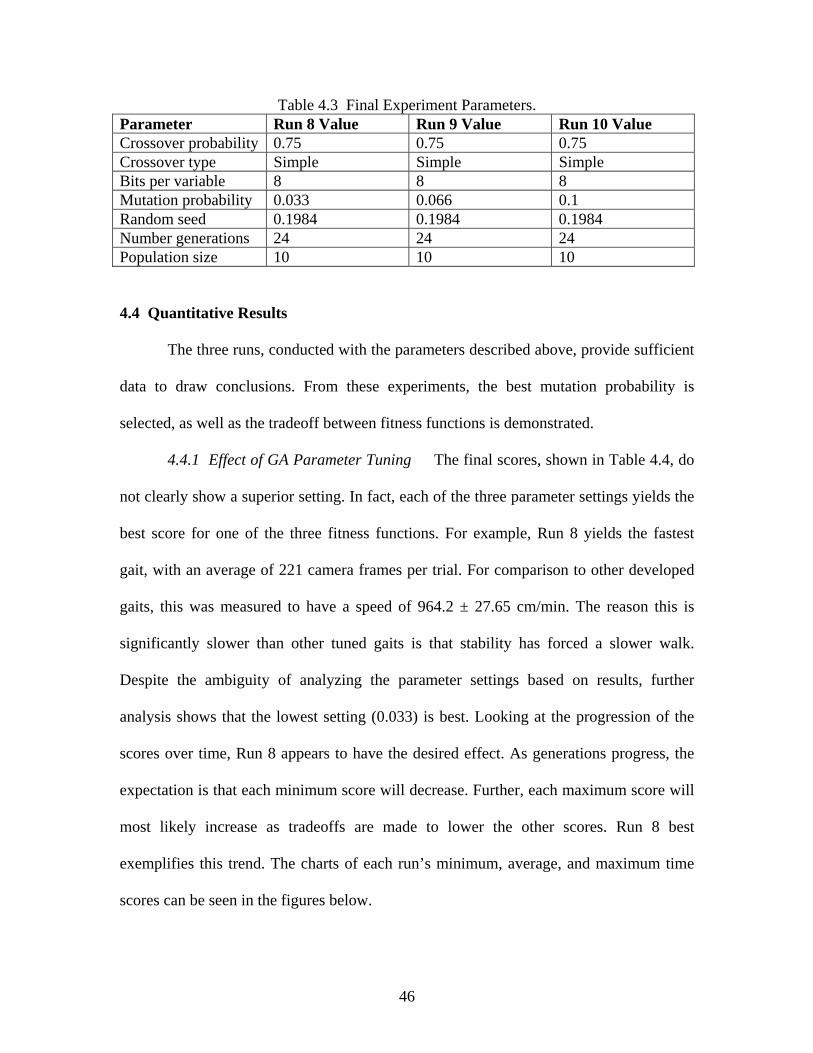
Table 4.3 Final Experiment Parameters. Parameter Run 8 Value Run 9 Value Run 10 Value Crossover probability 0.75 0.75 0.75 Crossover type Simple Simple Simple Bits per variable 8 8 8 Mutation probability 0.033 0.066 0.1 Random seed 0.1984 0.1984 0.1984 Number generations 24 24 24 Population size 10 10 10
4.4 Quantitative Results
The three runs, conducted with the parameters described above, provide sufficient
data to draw conclusions. From these experiments, the best mutation probability is
selected, as well as the tradeoff between fitness functions is demonstrated.
4.4.1 Effect of GA Parameter Tuning The final scores, shown in Table 4.4, do
not clearly show a superior setting. In fact, each of the three parameter settings yields the
best score for one of the three fitness functions. For example, Run 8 yields the fastest
gait, with an average of 221 camera frames per trial. For comparison to other developed
gaits, this was measured to have a speed of 964.2 ± 27.65 cm/min. The reason this is
significantly slower than other tuned gaits is that stability has forced a slower walk.
Despite the ambiguity of analyzing the parameter settings based on results, further
analysis shows that the lowest setting (0.033) is best. Looking at the progression of the
scores over time, Run 8 appears to have the desired effect. As generations progress, the
expectation is that each minimum score will decrease. Further, each maximum score will
most likely increase as tradeoffs are made to lower the other scores. Run 8 best
exemplifies this trend. The charts of each run’s minimum, average, and maximum time
scores can be seen in the figures below.
46
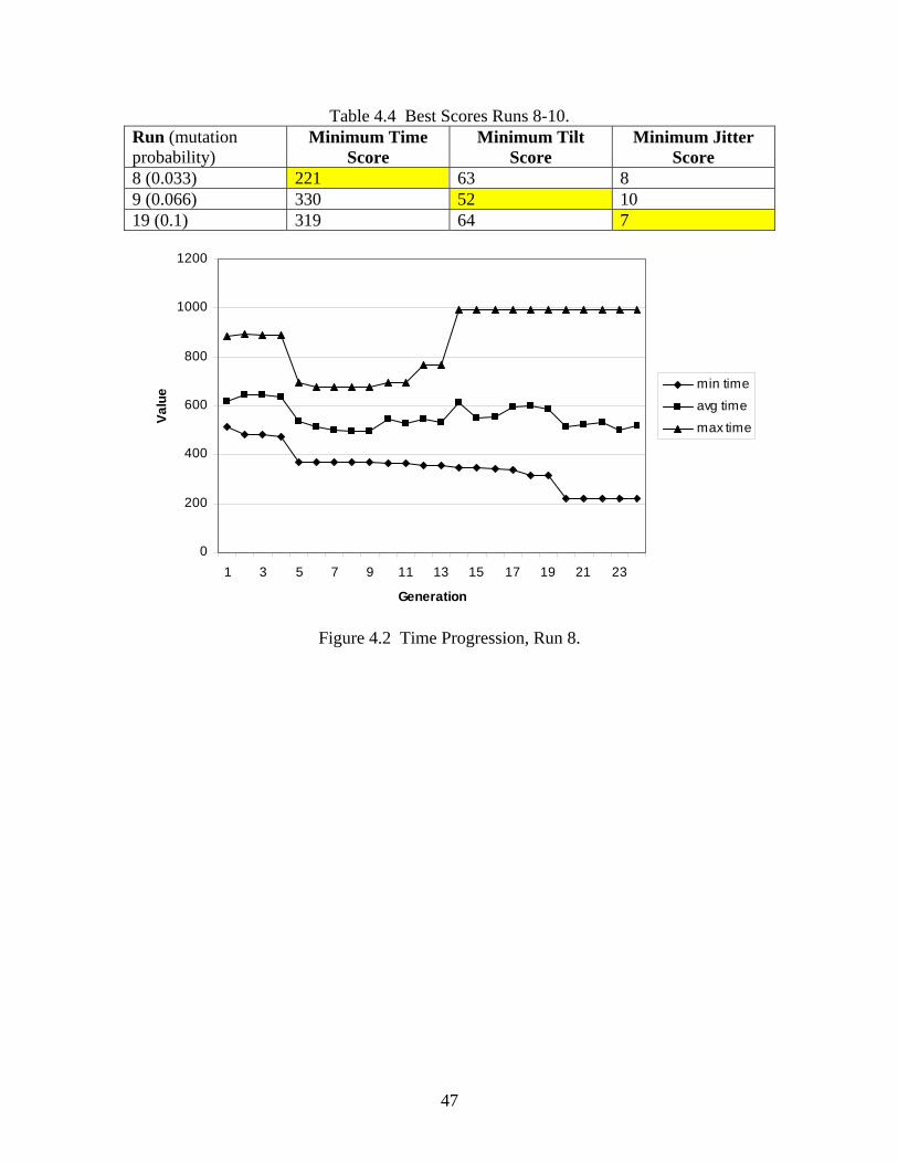
Table 4.4 Best Scores Runs 8-10. Run (mutation probability)
Minimum Time Score
Minimum Tilt Score
Minimum Jitter Score
8 (0.033) 221 63 8 9 (0.066) 330 52 10 19 (0.1) 319 64 7
0
200
400
600
800
1000
1200
1 3 5 7 9 11 13 15 17 19 21 23
Generation
Valu
e min time
avg time
max time
Figure 4.2 Time Progression, Run 8.
47
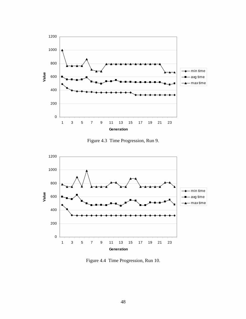
0
200
400
600
800
1000
1200
1 3 5 7 9 11 13 15 17 19 21 23
Generation
Valu
e min time
avg time
max time
Figure 4.3 Time Progression, Run 9.
0
200
400
600
800
1000
1200
1 3 5 7 9 11 13 15 17 19 21 23
Generation
Valu
e min time
avg time
max time
Figure 4.4 Time Progression, Run 10.
48

4.4.2 Nature of Trade-Off Between Fitness Functions Next, the tradeoffs
between the fitness functions are analyzed for trends. For clarity, projections onto two-
dimensional planes are presented here. The first projection is onto the time-jitter plane,
disregarding the tilt scores. Of the three data-collection runs, Run 8 provided the best
pareto front, which can be seen in Figure 4.5. Also, a composite of Runs 8, 9, and 10 are
shown in Figure 4.6. Here we can see a clear representation that speed and horizontal
stability are indeed competing goals. In general, as time decreases, jitter increases and
visa-versa. Further, we can see that this front appears to be smooth, with no distinctive
gaps of non-dominating scores along the pareto front.
0
10
20
30
40
50
60
0 200 400 600 800 1000 1200
Time
Jitte
r Dominated
Non-Dominated
Figure 4.5 Time-Jitter Tradeoff, Run 8.
49

0
10
20
30
40
50
60
0 200 400 600 800 1000 1200
Time
Jitt
er Dominated
Non-Dominated
Figure 4.6 Time-Jitter Tradeoff, Runs 8, 9, & 10.
The next projection deals with the tradeoff between jitter and tilt. For these fitness
functions, Run 10 provided the best pareto front. This data is presented in Figure 4.7, and
the composite data is shown in Figure 4.8. Again, one can see that jitter and tilt are
inversely proportional. As one increases, the other decreases. However, this pareto front
is not as evenly distributed as the previous one. Instead, the data clusters towards low
jitter and high tilt. Regardless, this tradeoff seems particularly interesting. Clearly the
property of stability is not unilateral. Also, it appears that some measure of instability is
inherent in all gaits. At some point, the aim must cease to be “minimize instability” and
become “allot instability optimally.”
50
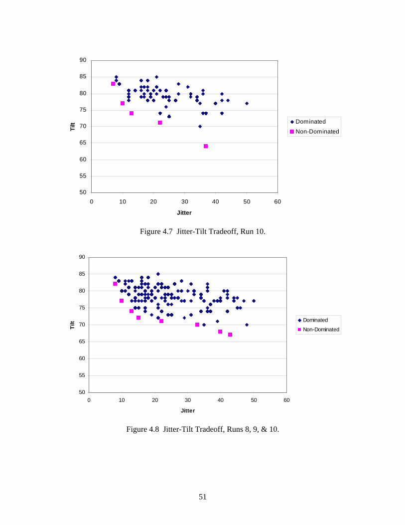
50
55
60
65
70
75
80
85
90
0 10 20 30 40 50 60
Jitter
Tilt Dominated
Non-Dominated
Figure 4.7 Jitter-Tilt Tradeoff, Run 10.
50
55
60
65
70
75
80
85
90
0 10 20 30 40 50 60
Jitter
Tilt Dominated
Non-Dominated
Figure 4.8 Jitter-Tilt Tradeoff, Runs 8, 9, & 10.
51
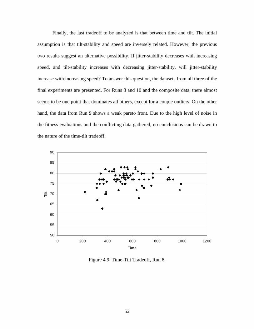
Finally, the last tradeoff to be analyzed is that between time and tilt. The initial
assumption is that tilt-stability and speed are inversely related. However, the previous
two results suggest an alternative possibility. If jitter-stability decreases with increasing
speed, and tilt-stability increases with decreasing jitter-stability, will jitter-stability
increase with increasing speed? To answer this question, the datasets from all three of the
final experiments are presented. For Runs 8 and 10 and the composite data, there almost
seems to be one point that dominates all others, except for a couple outliers. On the other
hand, the data from Run 9 shows a weak pareto front. Due to the high level of noise in
the fitness evaluations and the conflicting data gathered, no conclusions can be drawn to
the nature of the time-tilt tradeoff.
50
55
60
65
70
75
80
85
90
0 200 400 600 800 1000 1200
Time
Tilt
Figure 4.9 Time-Tilt Tradeoff, Run 8.
52

50
55
60
65
70
75
80
85
90
0 200 400 600 800 1000 1200
Time
Tilt
Figure 4.10 Time-Tilt Tradeoff, Run 9.
50
55
60
65
70
75
80
85
90
0 200 400 600 800 1000 1200
Time
Tilt
Figure 4.11 Time-Tilt Tradeoff, Run 10.
53

50
55
60
65
70
75
80
85
90
0 200 400 600 800 1000 1200
Time
Tilt
Figure 4.12 Time-Tilt Tradeoff, Runs 8, 9, & 10.
4.5 Empirical Observations
In addition to the quantitative results gathered throughout the experiments, many
qualitative observations were made that are worth noting. For instance, the
experimentation process had detrimental effects on the robot hardware. Also, effects of
learning were evident through observation, as well as factors that affected the fitness
scores.
4.5.1 Effects on the Robot First, experiments quickly deteriorate the robot’s
hardware. These observations give some insight into the effects on the robot that
deploying a gait of this type will have. During the experiments, one battery is good for
testing 20-30 gaits (dependant on gait speed and ability to reacquire the beacon after a
turn). Although the battery does not completely drained at this point (it still shows one of
three bars when replaced on the charger), there is a significant drop in motor power and
54

effectiveness, prompting a battery replacement. Because the battery is not completely
drained before being recharged, there is some concern over the battery developing a
memory and its charge depleting faster. Although no such deterioration was observed,
testing represented a relatively small fraction of the robot’s lifespan, and it is possible
such an effect will be come evident in the future.
Another impact on the robot comes as a result of the collision of the robot’s knees
and elbows. This, in addition to the repetitive movement of the joints, causes some slight
but noticeable wear on the robots’ motors. Development and initial testing was conducted
on one robot, which had to be switched out for later testing. Because this deterioration
was gradual, the true impact was not evident until the switch to new hardware had been
made. However, the development robot had been used in prior research, so not all wear is
attributable to this project.
Something else that proves to have a significant impact on the robot is the
temperature inside the laboratory. During the first set of experiments, the air conditioning
in the testing room was disabled, and the room grew very warm. When the air
conditioning was restored for the beginning of the second set of runs, the robot operated
significantly better. Specifically, the motors moved faster and stronger, the camera was
better able to recognize colors, and the battery life was extended. This means that instead
of testing 20-30 gaits on a single charge, 30-40 tests can be conducted in nearly the same
amount of time. Also, any temperature variation introduces noise into the speed
calculation.
4.5.2 Effects of Learning Empirical observations also showed that the genetic
algorithm was in fact improving the walk loci. Most obvious was that the walks speed up.
55

Generally, only gaits with the time parameter set to 4 and 7 are maintained in the
population. This represents those that were being kept for the speed score and those that
are being kept for the stability scores. Also, the length of the rear power stroke, which is
responsible for the majority of forward movement, seems to increase, resulting in a faster
gait.
Further, it appears that the walks become straighter over time as well. Although it
may be that systematic error is reduced as the experimenter gains experience, much of
this improvement should be contributed to learning. It was evident that straighter walks
score better because they keep the beacon in the center of the camera frame, reducing
jitter. It appears that the GA is able to pick up on this relationship throughout the
evolutionary process. Also, the GA may be able to recognize gaits that have a smoother
transition from the standing pose and favor them for survival as well.
4.5.3 Effects on Fitness Scores Probably the most significant effect on the
fitness evaluations is that the robot often gets turned away from the beacon and has to be
realigned by hand. There are several reasons for this behavior. The obvious first
explanation is that inconsistencies in the ground and robot lead to the robot not walking
completely straight. However, the impact of these variances appears to be eclipsed by the
fact that the robot is often misaligned from the beginning. One reason for this is that it
was difficult to place the robot perfectly in line between the two beacons by hand. The
second reason for misalignment, and the one with the largest impact, is the transition
from the standing pose to first walking pose. This is a quick movement to a non-
symmetrical pose. Although the angle shift was generally slight, it is often large enough
to have an impact after the robot walks a fair distance.
56

Although this behavior does not affect the speed measure significantly, it has a
much more significant impact on the two stability functions. For this reason, the robot is
manually realigned during the course of the trials. This leads to fitness scores that are
more reflective of the quality of the gait and influenced less by unimportant factors, such
as the robot’s initial alignment and the deflection caused when shifting out of the
standing pose. More reliable fitness scores are necessary if the genetic algorithm is to
produce gaits with better scores. Also, this manual manipulation is not overly intrusive
because the robot would have to correct for this under real-world conditions, regardless
of the causes. Further, because the speed function is not significantly impacted, it is clear
that this problem is unique to stability optimization.
Also worth noting are initial insights as to the stability of the camera for a
parameterized gait. From observation, it is clear that jitter has a bigger impact than tilt.
This is because the head, which houses the camera, shakes (yaw) with each step. Tilt,
however, is less of an issue because the robot’s design does not allow the head to roll
independently of the body. Therefore, all roll is in conjunction with the body or due to the
give in the neck construction, which is minor. The robot’s design allowes yaw of the
head, however. In fact, one of the degrees of freedom is the robot’s ability to yaw its
head. This means that a motor is holding the head in place, making it much easier to
disturb about the yaw axis than the roll axis. Further, the motor is placed at one end of the
head, so the motor has to overcome a significant amount of rotational inertia to stabilize
the head from yawing.
57

4.6 Summary
In summary, results show a clear tradeoff between the time and jitter scores as
well as between jitter and tilt. Despite the noise in the system and limited training data,
NSGA-II is able to evolve a pareto front and improve fitness scores. This project has also
helped characterize the nature of the domain through empirical observation. Notably, the
fitness functions are not only useful for creating pressure towards more stable gaits, but
straighter ones as well.
58

5. Conclusions and Future Work
This project is a success, as it meets all the objectives laid out at its onset. These
included developing a parameterized walk and a way to score gaits for speed and
stability. Further, this project sought to use a multi-objective genetic algorithm to evolve
gait parameters and provide results that would be analyzed for the speed-stability
tradeoff. A parameterized trot method was developed that moved the foot in a wheel like
motion. By defining two locus paths and a number of points to divide that path into, a
series of poses was created for the robot to assume, resulting in forward motion. Further,
two measures of stability, jitter and tilt, and a measure of speed were defined and
implemented. An experimental environment was developed in which the robot could test
the performance of each gait against these three fitness functions, using only onboard
sensors. Finally, a multi-objective genetic algorithm was tied in to the experimental
system using a wireless network connection. This GA allowed the development of three
large datasets, which were analyzed to gain a better understanding of tradeoffs between
the three fitness scores. The results showed a clear tradeoff between speed and stability,
in the form of jitter. As the time score increased from 221 to 827, the jitter score
decreased from 41 to 8. Also, a tradeoff between the two stability functions, jitter and tilt,
was also evident. Here, the tilt score increased from 64 to 83 as the jitter score decreased
from 37 to 7.
5.1 Future Work
The importance of camera stability for object recognition and a host of other tasks
has been previously established. Therefore, continuing research focused on the speed-
stability tradeoff may be critical. Such future work may take several forms, such as
59

improving the fitness functions, using different optimization techniques, automating the
process, and moving the head to track the beacon. Some specific topics in these areas are
discussed below.
5.1.1 Fitness Function Revision As mentioned above, the way stability was
measured and the reliability of those measures had a significant impact on the learning
process. Although the two fitness functions used in this project are representative of the
majority of camera instability, other functions may also prove useful. For example, the
jitter function used in this project only was concerned with horizontal displacement. One
other possible fitness function would be to consider the vertical jitter as well. The jitter
function(s) could be further refined by isolating offset by cause. For example, Figure 5.1
shows that offset can be caused by the twisting of the body while walking (A) or by
misalignment with the target (B). Also worth investigating would be the way these
distortions affect object recognition. For instance, is all jitter created equal? If two gaits
produce the same jitter score but one cycles faster than the other, is the slower cycle
better for object recognition?
60
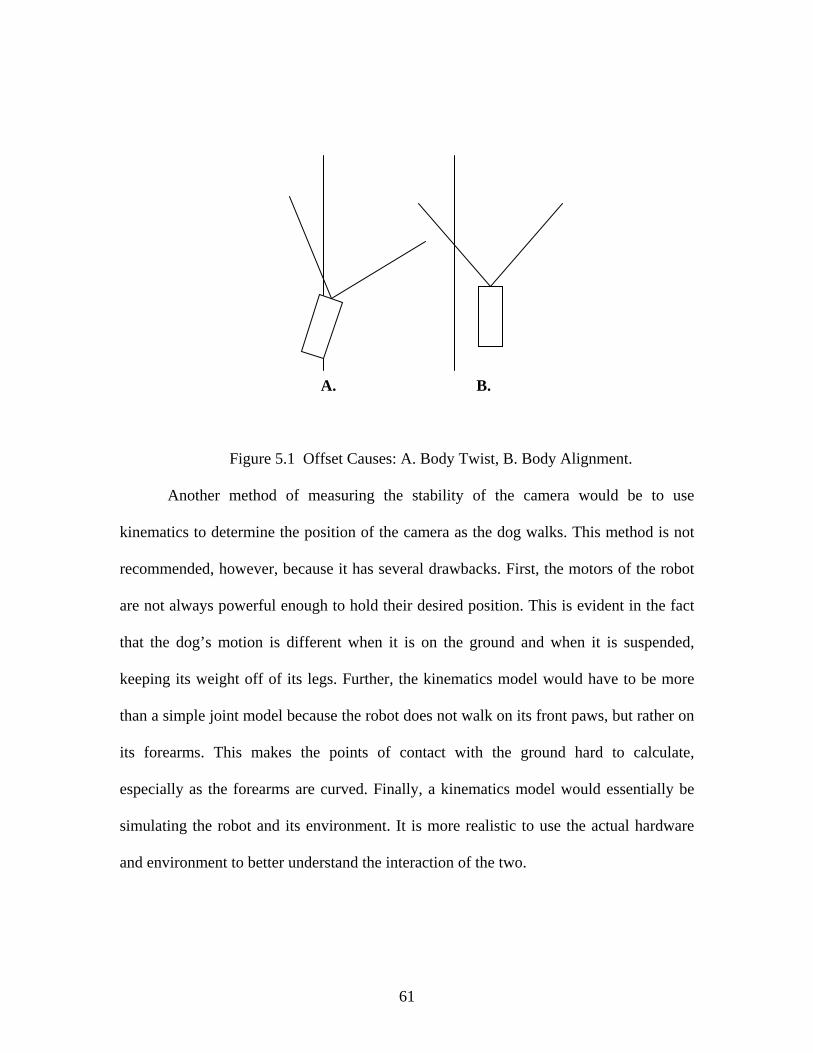
A. B.
Figure 5.1 Offset Causes: A. Body Twist, B. Body Alignment.
Another method of measuring the stability of the camera would be to use
kinematics to determine the position of the camera as the dog walks. This method is not
recommended, however, because it has several drawbacks. First, the motors of the robot
are not always powerful enough to hold their desired position. This is evident in the fact
that the dog’s motion is different when it is on the ground and when it is suspended,
keeping its weight off of its legs. Further, the kinematics model would have to be more
than a simple joint model because the robot does not walk on its front paws, but rather on
its forearms. This makes the points of contact with the ground hard to calculate,
especially as the forearms are curved. Finally, a kinematics model would essentially be
simulating the robot and its environment. It is more realistic to use the actual hardware
and environment to better understand the interaction of the two.
61

5.1.2 Optimization Method Another area for future work lies in improving the
optimization methods used to generate the pareto front. The most basic of these methods
is further tuning of the parameters of the genetic algorithm. Although crossover rate,
mutation rate, population size, and number of generations were experimented with, bit
length representation was not. Further, the changes to the parameters were quite cursory.
Fine tuning of these parameters may increase the quality of the pareto front and solutions
generated. Second, other optimization methods could be used, such as linear
programming or discrete methods.
5.1.3 Automation One of the major limitations of this project was the inability
to collect large amounts of data. Because each experiment lasted for over twelve hours,
time was the major limitation, although hardware degradation also played a factor. The
best way to mediate this inhibition would be to automate the testing process. In this way,
tests could be run in parallel, or, at the very least, in a more continuous manner, given the
same amount of manpower.
Despite the obvious advantages to automation the testing process, this proved to
be outside the scope of this project. The principal hurdle to automating this process is
getting the robot to turn around and reset itself for the next trial. First, more color
detection tables would have to be defined so that the robot would be able to distinguish
between the two beacons. Next, a more effective turning motion would have to be
developed. This, however, may not be too complicated as the original presentation of a
parameterized walk [11] claimed that a gait is effective in turning and strafing, in
addition to forward and backward motion. In fact, the ability to be used to turn may even
become another fitness measure, although it is unclear how this would be measured on
62
the robot. Also, the wireless communication between the robot and computer would have
to be corrected and a way developed to pause the genetic algorithm to enable battery
changes. Finally, the robot would have to be able to detect and correct when it has veered
off course. Otherwise, the angular errors compound and corrupt the fitness scores.
5.1.4 Head Stabilization Another way to enhance the camera stability would be
to move the head in order to counter the motion induced by the body. Although this
method has its drawbacks, it may prove helpful. For instance, the robot has no control
over the roll of its head, so it will only be able to counter yaw. However, as mentioned
previously, yaw, and hence horizontal jitter, seems to be the major source of instability.
Also, there will be times when the robot is looking around and will be unable to focus on
one object. Nevertheless, this method will be able to improve the ability of the robot to
track an object once it has acquired one. There are two apparent ways to implement such
stabilization. First, it is possible to explicitly code a program to move the head towards
the center of an object. In fact, this is one of the sample programs provided with the
OPEN-R SDK, albeit the most complicated example. The other approach would be to
learn the head movement in addition to the gait. This is the method used by the UT
Austin team. Although they had little success learning the head motion in conjunction
with the gait, it is likely that the process would be more successful if the gait was learned
independently and then the head motion learned in a second iteration to be custom fitted
to the chosen gait.
5.3 Conclusions
Despite camera stability’s and speed’s impact on several higher-level robot tasks,
little work has been done, until now, to understand the nature of the tradeoff between
63

these two competing goals. Building off the previous methods for increasing the speed of
the AIBO’s trot, this project has established a method for increasing both the speed and
stability of a selected gait. More importantly, however, data has been collected to chart
the tradeoff between speed and two stability components, jitter and tilt, for the first time.
64

Appendix A. Data for Figure 4.5
Table A.1 Non-Dominated Points (Based on Time-Jitter projection), Run 8. Parameter Values Points per stroke 4 5 5 5 6 8 8 8 Front 1 o’clock X 70 70 73 73 74 73 74 74 Front 1 o’clock Y 54 54 54 54 42 40 43 43 Front 1 o’clock Z 9 9 14 14 14 14 14 14 Front 4 o’clock X 81 84 84 84 83 89 84 84 Front 4 o’clock Y 64 64 61 61 61 61 61 61 Front 4 o’clock Z 18 18 19 19 9 20 19 19 Front 7 o’clock X 11 11 21 24 24 11 21 24 Front 7 o’clock Y 62 62 59 59 49 60 60 57 Front 7 o’clock Z 3 4 1 4 4 1 1 1 Front 11 o’clock X 48 48 39 48 48 34 39 39 Front 11 o’clock Y 44 44 54 54 54 54 54 54 Front 11 o’clock Z 16 17 14 14 15 14 14 14 Rear 1 o’clock X 27 27 18 13 13 13 13 -2 Rear 1 o’clock Y 77 77 78 88 78 78 78 78 Rear 1 o’clock Z 19 19 9 7 17 9 9 9 Rear 4 o’clock X 26 26 11 11 12 11 11 21 Rear 4 o’clock Y 116 116 103 103 103 101 103 103 Rear 4 o’clock Z 2 2 15 15 15 16 15 10 Rear 7 o’clock X -68 -68 -55 -65 -65 -65 -55 -34 Rear 7 o’clock Y 115 115 109 104 104 104 104 104 Rear 7 o’clock Z 9 8 8 8 8 8 8 8 Rear 11 o’clock X -57 -57 -56 -69 -66 -59 -56 -57 Rear 11 o’clock Y 92 92 92 95 95 95 92 92 Rear 11 o’clock Z 13 13 13 13 13 10 13 13 Time Score 221 314 438 511 529 606 675 827Tilt Score 71 73 81 83 79 80 80 82Jitter Score 41 24 15 13 12 11 10 8
65

Appendix B. Data for Figure 4.7
Table B.1 Non-Dominated Points (Based on Jitter-Tilt projection), Run 10. Parameter Values Points per stroke 4 6 8 8 5Front 1 o’clock X 61 93 96 98 65Front 1 o’clock Y 42 40 46 43 41Front 1 o’clock Z 3 11 9 6 1Front 4 o’clock X 89 90 89 90 96Front 4 o’clock Y 62 59 62 58 61Front 4 o’clock Z 9 1 9 5 3Front 7 o’clock X 23 35 14 36 11Front 7 o’clock Y 60 55 60 56 62Front 7 o’clock Z 8 7 3 2 3Front 11 o’clock X 21 47 21 42 25Front 11 o’clock Y 53 59 53 57 43Front 11 o’clock Z 10 12 10 1 12Rear 1 o’clock X -7 15 13 8 18Rear 1 o’clock Y 79 91 79 88 75Rear 1 o’clock Z 4 9 9 8 9Rear 4 o’clock X 11 12 11 25 17Rear 4 o’clock Y 102 108 101 102 108Rear 4 o’clock Z 11 17 12 8 16Rear 7 o’clock X -59 -67 -68 -43 -69Rear 7 o’clock Y 116 101 116 113 116Rear 7 o’clock Z 14 18 14 16 11Rear 11 o’clock X -49 -40 -46 -42 -46Rear 11 o’clock Y 76 91 91 81 91Rear 11 o’clock Z 1 2 7 13 7 Time Score 540 463 511 616 326Tilt Score 64 71 74 77 83Jitter Score 37 22 13 10 7
66

Bibliography
[1] Beer, Randall D. and John C. Gallagher. \Evolving dynamical neural networks for
adaptive behavior”. Adapt. Behav., 1(1):91-122, 1992. ISSN 1059-7123.
[2] Capi, G.; Yokota, M.; Mitobe, K., "A New Humanoid Robot Gait Generation
Based on Multiobjective Optimization," Advanced Intelligent Mechatronics.
Proceedings, 2005 IEEE/ASME International Conference on , vol., no., pp. 450-
454, 2005.
[3] Chernova, S. and Veloso, M. (2004). An Evolutionary Approach To Gait
Learning For Four-Legged Robots. Proceedings of IEEE/RSJ International
Conference on Intelligent Robots and Systems. 3:2562- 2567.
[4] Deb, K., Paratap, A., Agarwal, S. and Meyarivan, T. (2002). A Fast and Elitist
Multiobjective Genetic Algorithm: NSGA-II. In IEEE Transactions on
Evolutionary Computation, 6(2):182-197.
[5] Fonseca, C. M. and Fleming, P. J. (1998). Multiobjective Optimization and
Multiple Constraint Handling with Evolutionary Algorithms – Part I: A Unified
Formulation. IEEE Transactions on Systems, Man and Cybernetics – Part A:
Systems and Humans, 28(1):26-37.
[6] Fujii, Akinobu, Akio Ishiguro, Takeshi Aoki, and Peter Eggenberger. “Evolving
Bipedal Locomotion with a Dynamically-Rearranging Neural Network”. ECAL
'01: Proceedings of the 6th European Conference on Advances in Articial Life,
509-518. Springer-Verlag, London, UK, 2001.
67

[7] G. Oh, C.K. Barlow, “Autonomous controller design for unmanned aerial vehicles
using multi-objective genetic programming,” in Evolutionary Computation, 2004.
CEC2004. Congress on, vol. 2, 2004, pp. 1538–1545.
[8] Goldbert, D. E. (1989). Genetic Algorithms in Search, Optimization, and Machine
Learning. Addisoin Wesley, Reading, MA.
[9] Golubovic, D. and Hu, H. (2003). Parameter Optimisation of an Evolutionary
Algorithm for On-line Gait Generation of Quadruped Robots. Proceedings of
IEEE International Conference on Industrial Technology.
[10] H. Teo, J. Abbass, “Coordination and synchronization of locomotion in a virtual
robot,” in Neural Information Processing, 2002. ICONIP ’02. Proceedings of the
9th International Conference on, vol. 4, November 2002, pp. 1931–1935.
[11] Hengst, B., Ibbotson, D., Pham, S. B. and Sammut, C. (2002). Omnidirectional
Locomotion for Quadruped Robots. RoboCup 2001: Robot Soccer World Cup V.
2377: 368 – 373.
[12] Hengst, Bernhard et al. (2000). The UNSW United 2000 Sony Legged Robot
Software System. School of Computer Science and Engineering, University of
New South Wales. http://www.cse.unsw.edu.au/~robocup/2005site/reports.phtml
72-74.
[13] Horn, J., Nafpliotsis, N., and Goldberg, D. E. (1994). A Niched Pareto Genetic
Algorithm for Multiobjective Optimization. In Michalewicz, Z., editor,
Proceedings of the First IEEE Conference on Evolutionary Computation, pages
82-87, Piscataway NJ. IEEE Service Center.
68

[14] Hornby, G. S., Takamura, S., Yamamoto, T. and Fujita, M. (2005). Autonomous
Evolution of Dynamic Gaits with Two Quadruped Robots. IEEE Transactions on
Robotics. 3:402-410.
[15] Hornby, G. S., Takamura, S., Yokono, J., Hanagata O., Yamamoto, T. and Fijita,
M. (2000). Evolving Robust Gaits with AIOB. Proceedings of IEEE International
Conference on Robotics and Automation. 3:3040-3045.
[16] J. S. C. J. C. Jiapin, “Design of central pattern generator for humanoid robot
walkingbased on multi-objective ga,” in Intelligent Robots and Systems, 2000.
(IROS 2000). Proceedings. 2000 IEEE/RSJ International Conference on, vol. 3,
2000, pp. 1930–1935.
[17] Jackson, R. H. F., Boggs, P. T., Nash, S. G., and Powell, S. (1991). Guidelines for
Reporting Results of Computational Experiments – Report of the Ad Hoc
Committee. Mathematical Programming, 49:413-425.
[18] Kim, M. S. and Uther, W. (2003). Automatic Gait Optimisation for Quadruped
Robots. Australasian Conference on Robotics and Automation.
[19] Kleeman, M. P., Lamont, G. B., Cooney, A. and Nelson, T. R. A Parallel
Memetic Multiobjective Evolutionary Algorithm for the Design of Quantum
Cascade Lasers.
[20] Knowles, Joshua and David Corne. “The Pareto Archived Evolution Strategy: A
New Baseline Algorithm for Pareto Multi-Objective Optimization". Peter J.
Angeline, Zbyszek Michalewicz, Marc Schoenauer, Xin Yao, and Ali Zalzala
(editors), Proceedings of the Congress on Evolutionary Computation, volume 1,
69
98-105. IEEE Press, Mayflower Hotel, Washington D.C., USA, 6-9 1999. ISBN
0-7803-5537-7 (Microfche). URL citeseer.ist.psu.edu/knowles99pareto.html.
[21] Kodjabachian, Jean-Arcady, Jerome; Meyer. “Evolution and Development of
Modular Control Architectures for 1D Locomotion in Six-legged Animals".
Connection Science, 10.3:211{237, September 1998. URL
http://www.informaworld.com/10.1080/095400998116413.
[22] Kohl, N. and Stone, P. (2004). Machine Learning for Fast Quadrupedal
Locomotion. Proceedings of the Nineteenth National Conference on Artificial
Intelligence.
[23] Kohl, N. and Stone, P. (2004). Policy Gradient Reinforcement Learning for Fast
Quadrupedal Locomotion. Proceedings of IEEE International Conference on
Robotics and Automation. 3:2619-2624.
[24] “OPENR-SDK: Model Information for ERS-7”. Sony Corporation, 2004. URL
http://www.openr.org/.
[25] Otsu, Ishiguro A.-Aoki T., K. and P. Eggenberger. “Evolving an Adaptive
Controller for a Quadruped-Robot with Dynamically-Rearranging Neural
Networks". International Conference on Intelligent Robots and Systems. 2001.
[26] P. K. Deb, “Kanpur genetic algorithms laboratory,”
http://www.iitk.ac.in/kangal/codes.shtml, August 2006, nsga2code.tar.
[27] “PWalk.cc”. University of New South Wales, 2003. URL
http://www.cse.unsw.edu.au/~robocup/2005site/reports.phtml.
70
[28] Quinlan, M. J., Chalup, S. K. and Middleton, R. H. (2003). Techniques for
Improving Vision and Locomotin on the Sony AIBO Robot. Australasian
Conference on Robotics and Automation.
[29] Reeve, Richard. Generating walking behaviors in legged robots. Ph.D. thesis,
University of Edinburgh, Scotland, 1999.
[30] Reil, Torsten and Phil Husbands. “Evolution of central pattern generators for
Bipedal walking in a real-time physics environment". IEEE Trans. Evolutionary
Computation, 6(2):159-168, 2002.
[31] Reil, T. and C. Massey. “Biologically Inspired Control of Physically Simulated
Bipeds”. Theory in Biosciences, 120:327-339, 2001.
[32] Richard O. Day, Mark P. Kleeman and Gary B. Lamont. “Multi-Objective fast
messy Genetic Algorithm Solving Deception Problems”. Congress on
Evolutionary Computation., 2:1502-1509, 2004.
[33] RoboCup website. http://www.robocup.org/, 2006.
[34] Saggar, M., D’Silva, T., Kohl, N. and Stone, P. (2007) Autonomous Lerning of
Stable Quadruped Locomotion. To appear in RoboCup-2006: Robot Soccer World
Cup X.
[35] Serra, Francois and Jean-Christophe Baillie. Aibo programming using OPEN-R
SDK Tutorial. Technical report, ENSTA, 2003. URL
http://www.ensta.fr/baillie/tutorialOPENRENSTA-1.0.pdf.
[36] Srinivas, N. and Deb, K. (1994). Multiobjective Optimization Using
Nondominated Sorting in Genetic Algorithms. Evolutionary Computation,
2(3):221-248.
71

72
[37] “stand.pse”. Sony Corporation, 2004. MEdit for ERS-7 1.0.7.
[38] Teo, J. (2004). Darwin + Robots = Evolutionary Robotics: Challenges in
Automatic Robot Synthesis. Proceedings of the 2nd International Conference on
Artificial Intelligence in Engineering and Technology. Kota Kinabalu, Sabah,
Malaysia. 1:7-13.
[39] Van Veldhuizen, D. A. (1999). Multiobjective Evolutionary Algorithms:
Classification, Analyses, and New innovations. PhD Thesis, AFIT/DS/ENG/99-
01, Air Force Institute of Technology, Wright-Patterson AFB.
[40] Van Veldhuizen, D. A. and Lamont, G. B. (2000). Multiobjective Optimization
with Messy Genetic Algorithms. In To Appear in the Proceedings of the 2000
ACM Symposium on Applied Computing. ACM.
[41] Van Veldhuizen, D. A. and Lamont, G. B. (2000). On Measuring Multiobjective
Evolutionary Algorithm Performance. Proceedings of 2000 Conference on
Evolutionary Computation. 1:204-211.
[42] Wang, Zheng et al. (2002) rUNSWift: UNSW RoboCup2002 Sony Legged
League Team. University of New South Wales. Ch 5.
[43] Wijbenga, Anton and Mart Van De Sanden. “How To Make AIBO Do Tricks”,
2004.
[44] Zitzler, E. Evolutionary Algorithms for Multi-Objective Optimization: Methods
and Applications. Ph.D. thesis, Swiss Federal Institute of Technology Zurich,
2000.
REPORT DOCUMENTATION PAGE Form Approved OMB No. 074-0188
The public reporting burden for this collection of information is estimated to average 1 hour per response, including the time for reviewing instructions, searching existing data sources, gathering and maintaining the data needed, and completing and reviewing the collection of information. Send comments regarding this burden estimate or any other aspect of the collection of information, including suggestions for reducing this burden to Department of Defense, Washington Headquarters Services, Directorate for Information Operations and Reports (0704-0188), 1215 Jefferson Davis Highway, Suite 1204, Arlington, VA 22202-4302. Respondents should be aware that notwithstanding any other provision of law, no person shall be subject to an penalty for failing to comply with a collection of information if it does not display a currently valid OMB control number. PLEASE DO NOT RETURN YOUR FORM TO THE ABOVE ADDRESS. 1. REPORT DATE (DD-MM-YYYY)
13-09-2007 2. REPORT TYPE
Master’s Thesis 3. DATES COVERED (From – To)
Sept 2006 – Sept 2007 5a. CONTRACT NUMBER
5b. GRANT NUMBER
TITLE AND SUBTITLE MULTI-OBJECTIVE OPTIMIZATION FOR SPEED AND STABILITY OF A SONY AIBO GAIT
5c. PROGRAM ELEMENT NUMBER
5d. PROJECT NUMBER 5e. TASK NUMBER
AUTHOR(S) Patterson, Christopher, 2nd Lieutenant, USAF 5f. WORK UNIT NUMBER
7. PERFORMING ORGANIZATION NAMES(S) AND ADDRESS(S) Air Force Institute of Technology Graduate School of Engineering and Management (AFIT/EN) 2950 Hobson Way, Building 640 WPAFB OH 45433-8865
8. PERFORMING ORGANIZATION REPORT NUMBER AFIT/GCS/ENG/07-17
10. SPONSOR/MONITOR’S ACRONYM(S)
9. SPONSORING/MONITORING AGENCY NAME(S) AND ADDRESS(ES) Dr. Jacob Campbell, AFRL/SNRN 2241 Avionics Circle, Bldg 620, Room 3AJ39 Wright-Patterson AFB, OH 45433-7333 (937) 255-6127x4154 [email protected]
11. SPONSOR/MONITOR’S REPORT NUMBER(S)
12. DISTRIBUTION/AVAILABILITY STATEMENT APPROVED FOR PUBLIC RELEASE; DISTRIBUTION UNLIMITED.
13. SUPPLEMENTARY NOTES 14. ABSTRACT Ant colony optimization algorithms have long been touted as providing an effective and efficient means of generating high quality solutions to NP-hard optimization problems. Unfortunately, while the structure of the algorithm is easy to parallelize, the nature and amount of communication required for parallel execution has meant that parallel implementations developed suffer from decreased solution quality, slower runtime performance, or both. This thesis explores a new strategy for ant colony parallelization that involves Area of Expertise (AOE) learning. The AOE concept is based on the idea that individual agents tend to gain knowledge of different areas of the search space when left to their own devices. After developing a sense of their own expertness on a portion of the problem domain, agents share information and incorporate knowledge from other agents without having to experience it firsthand. This thesis shows that when incorporated within parallel ACO and applied to multi-objective environments such as a gridworld, the use of AOE learning can be an effective and efficient means of coordinating the efforts of multiple ant colony agents working in tandem, resulting in increased performance. 15. SUBJECT TERMS
Artificial intelligence; Robotics; Sony AIBO; Quadruped gait optimization; Camera stability; Multi-objective optimization; Multi-objective Genetic Algorithms.
16. SECURITY CLASSIFICATION OF:
19a. NAME OF RESPONSIBLE PERSON Gilbert L. Peterson, PhD (ENG)
a. REPORT
U
b. ABSTRACT
U
c. THIS PAGE
U
17. LIMITATION OF ABSTRACT
UU
18. NUMBER OF PAGES
82
19b. TELEPHONE NUMBER (Include area code) (937) 255-6565, ext 4281 ([email protected])
Standard Form 298 (Rev. 8-98) Prescribed by ANSI Std. Z39-18