The calculus of variations in the large

By Marston Morse, Cambridge, U. S. A.

Introduction. The theory to be presented here may be described as the analogue for functionals of the author's theory9 of critical points5 of a function / of n variables. The latter theory proceeds by virtue of three principal steps.

(I). The determination of the topological characteristics of the domain R of definition of the function.

(2). The assignment of type numbers to the critical sets. (3). The determination of the relations between the topological characteristics

of R and the type numbers of the critical sets of /. Relative to step (1) we say simply that for functions (but not for functionals) an

adequate topological theory is already at hand. Relative to step (2) we remark that in case the function is analytic and the

domain is a finite, analytic, regular w-manifold without boundary, the critical sets are necessarily finite in number. In case a critical set is an isolated point P and the hessian of / does not vanish at P (the non-degenerate case) type numbers Mk are assigned by the author to P as follows. Let k be the index of the quadratic form whose coefficients are the elements of the hessian of / at P. Corresponding to P we take all of the type numbers as zero except Mk and take Mk as 1. In the case of the general critical set CD, type numbers are assigned to co in a way which is a generali­zation of the assignment in the non-degenerate case. If N{ is now the sum of the type numbers Mi assigned to the different critical sets co of /. we have shown that

(o.i) Nt ;> B{

where Rt is the âth connectivity (mod. 2) of the domain R. The assignment of type numbers to the general critical set co is one which has the following remarkable property. If the function / is approximated sufficiently closely by a non-degenerate function F (one whose critical points are all non-degenerate), there will always appear, neighboring a critical set of /, a set of isolated, non-degenerate critical points of F whose type number sums E Mi are at least as great as the respective numbers Mi

which we have assigned to co. Moreover it can be shown that the function / can always be approximated by a non-degenerate function F.

The relations (0.1) establish the existence of the topologically necessary critical points. If N{ > Ri for a particular i, we say that there exists an excess of critical points of index i. This excess is not arbitrary. In fact the numbers Nf and Ri must satisfy the relations

173

Grosse Vorträge

N0Ì?R0

No — N, ^R0~R1

(0.2) No — ^ + Nt ^RQ — R1 + R2

N0 — N±+ ... +(r-i)nNn = B0 — R1+ ... + ( _ i ) » Ä n .

We call the relations (0.2) limitations on the excess of critical points16. These relations are complete in a sense upon which we shall not here enlarge.

We now turn to the calculus of variations. Corresponding to a given set of boundary conditions B, we shall regard a Jordan arc which satisfies the conditions B as a point in function space. The conditions B might, for example, require the end points of the arc to be fixed, or to He on two end manifolds. The totality of the Jordan arcs satisfying conditions B will be termed the functional domain Q asso­ciated with B. Step (1) now calls for new developments. We proceed by defining bounding on Ü, cycles on Q, and the connectivities Ri of Q (i = 0, 1, . . . ). In con­trast with ordinary topology we find that infinitely many of the connectivities of Q are in general not null.

One naturally replaces the function / by the calculus of variations integral, and the critical points of / by critical extremals, that is, extremals satisfying the trans-versality conditions associated with the boundary problem B. We restrict ourselves to the analytic case. Basic critical sets co are here maximal sets of critical extremals, mutually deformable into one another among extremals of co. We solve the difficult problem of characterizing the non-degenerate critical point and of assigning type numbers to each critical set. In general there will be infinitely many critical sets. The value of the integral on extremals of a critical set co will be constant. In the analytic case the critical values will be isolated.

Whereas the type numbers of a critical set co of an ordinary function / consist of a set of n + 1 numbers, here the type numbers of co consist of an infinite set of numbers

M0, Mx, ...

For any particular set co all but a finite subset of these numbers M{ will be null. But the indices i of the non-null type numbers Mt in general will not be bounded for all critical sets co of the problem. This corresponds to the fact tha t the indices i of non-null connectivities Ri of the function manifold Ü are in general not bounded, and that the relations (0.1) still hold. These relations are very powerful and will in general prove the existence of infinitely many critical extremals. The limitations (0.2) on the excess of critical extremals now become an infinite set of inequalities of the same form and produce a host of remarkable relations.

As a matter of pure topology, the connectivities of our functional domain reduce

174

Marston Morse: The calculus of variations in the large

upon suitable specialization of the boundary conditions and the integral to the ordinary connectivities of an ordinary manifold, or if we please, to the connectivities of a product manifold. Other simple specializations are possible.

The present paper is necessarily limited. The special case of the periodic extremal is not treated here. References to that part of the theory which has been published are given at the end. A more complete treatment will be given in the Colloquium Lectures on "The Calculus of Variations" given in September, 1931 and to be publish­ed shortly. Other references are given at the end.

l.An integral on a Riemannian space. In this section we shall give a definition of a Riemannian space in the large and define an integral thereon.

Riemannian spaces as ordinarily defined are local affairs. I t is necessary for us to add topological structure in the large. To that end we suppose tha t we have given an ordinary m-dimensional simplicial circuit Km in an auxiliary Euclidean space on which the neighborhood of each point is well defined. (See Lefschetz ref. 13.) Our Riemannian space R will now be defined as follows. I ts points and their neigh­borhoods shall be the one-to-one images of the respective points and their neigh­borhoods on K. Moreover Km shall be of such nature that the neighborhood of each of its points is homeomorphic with the neighborhood of a point (x) in an Euclidean m-space of coordinates (x) = (xl9 . .., xm). With at least one such representation of the neighborhood of a point of R there shall be associated a positive definite Riemannian form

(1.1) ds2 = gu (x) dx* dx> (i, j) = (1, . . . , m)

defining a metric14 for the neighborhood. For simplicity we suppose that the coef­ficients g^( x) are analytic. We term the coordinates (x) admissible. We also admit any other set of local coordinates (z) obtainable from admissible coordinates (x) by a transformation of the form

(1.2) zl = zl (x)9

defined by functions zi (x) analytic in (#) and possessing a non-vanishing Jacobian. We require that any two coordinate systems (x) and (z) which admissibly represent the neighborhood of the same point P must be related as in (1.2). We term (1.2) an admissible transformation of coordinates.

A set of points of R will be said to form a regular analytic n-manifold on R if the images of its points in any local coordinate system (x) is locally representable in the form

xi = x* (ul9 ...,un)

where the functions x* (u) are analytic in the parameters (u) and the functional ma­trix of the functions x* (u) is of rank n.

175

Grosse Vorträge

With each admissible coordinate system (x) we suppose tha t we have given a function

F (x, r) = F (x1, ...,xm,r\ ..., rm) (r) ± (0)

serving to define an invariant integral

fF(x,x)dt

in that system, where x* represents the derivative of x* with respect to a para­meter t.

For at least one admissible coordinate system neighboring each point of R (and consequently for all such coordinate systems) we assume tha t the corresponding integrand is positive and analytic in (x) and (r) for (r) =}= (0). We also assume that F (x, r) is positively homogeneous of order 1 in the variables (r), as in the classical theory of Weierstrass. We further assume that the form

(1.3) Frirj (s,r)A<A' (i,j= 1, ...,m)

is positive for unit vectors (À) 4= M-2. The functional domain and its connectivities. Let A1 and A2 be any two distinct

points on R. The points A1 and A2 are to serve as the initial and final points respec­tively of admissible curves. Locally we represent A1 and A2 by sets of coordinates

(x) = (x11, ..., xml) (x) = (x12, . . ., xm2)

respectively. Let Br be an auxiliary simplicial r-cycle with 0 <J r < 2m. Suppose that we have a set of pairs of points (A1, A2) homeomorphic with Br. We understand that A1 =t= A2 and tha t A1 and A2 lie on R. For r > 0 we suppose that the neighborhood of each point of Br can be represented as the one-to-one continuous image of a neigh­borhood of a point (a0) in our auxiliary Euclidean r-space of r coordinates (a) and that the corresponding points (A1, A2) can be locally represented in the form

xis _ xis ^ (i _ ^ m . s _ i 5 2)

where the functions xis (a) are analytic in (a) for (a) near (aQ) and possess a functional matrix of rank r. We call this set of points (A1, A2) the terminal manifold Z.

Let y be a sensed Jordan arc on R on which a parameter t runs from 0 to 1 inclusive. If the respective end points of y determine a point (A1, A2) on Z, y will be termed topologically admissible. When we are dealing with our integral we shall suppose that y is of class Z^as well as topologically admissible. We then term y a restricted curve. Evaluated on restricted curves the integral defines our basic func­tional J.

The totality of topologically adînissible curves will be termed the functional domain Q corresponding to the space R and terminal manifold cape.

176

Marston Morse: The calculus of variations in the large

By a /-complex 1cj on Ü we mean a /-parameter family of curves of Q given as the continuous map of the product c, X t of an auxiliary /-complex Cj, and the line seg­ment 0 f£ t ^ 1, with each curve y corresponding to the product of a point of Cj and the line segment. As in the theory of singular complexes we regard points on these curves as distinct if they are images of distinct points on Cj X t. In this family the curves corresponding to the product of a /-cell of Cj and the line segment t will define a family of curves which we call a &-cell of kj. To subdivide 1cj we subdivide Cj.

The boundary of 1cj (mod. 2) shall be the (/— 1) -complex on Ü which is the image in the above map of the product of the boundary (mod. 2) of Cj and the line segment 0 <£ t =g 1. A /-complex on Ü will be termed a /-cycle if without boundary. A set of /-cycles on Q is termed homologous to zero if the cycles of the set form the boundary of a (/ + l)-complex on Ü. Everything is to be understood mod. 2. We see that the usual operations with homologies are permissible.

By the connectivity Pj of Q, j = 0, 1, . . . we mean the maximum number of /-cycles on Q between which there is no homology, provided such a maximum exists. If no such maximum exists we say that Pj is infinite.

The connectivities of Q are invariant under any topological transformation of R which carries admissible end points (A1, A2) into admissible end points. For pur­poses of pure topology the analyticity of R and Z is of course unessential.

3. The function J (II). I t is well known that there exists a positive constant e, small enough to have the following properties. Any extremal arc E on which J < e will give an absolute minimum to J relative to all sensed curves of class D1 joining E's end points. On E the local coordinates of any point will be analytic functions of the local coordinates of the end points of E and of the distance of P along E from the initial end point Q of E, at least as long as E does not reduce to a point. The set of all extremal segments issuing from Q with J < e will form a field covering a neighborhood of Q in a one-to-one manner, Q alone excepted. We now choose a positive constant Q less than e and make the following definition.

Any extremal segment on R for which J is less than Q will be called an elementary extremal.

An ordered set of p + 2 points

(3.1) A\P\ ...,PP,A*

on R with (A1, A2) on the terminal manifold will be denoted by (77). The points (3.1) will be called the vertices of (II). I t may be possible to join the successive points in (3.1) by elementary extremals. In such a case (II) will be termed admissible. The resulting broken extremal will be denoted by g (77) and also termed admissible. The value of J taken along g (77) will be denoted by J (77).

Let a copy of R be provided for each point P \ Points (77) can be represented as

12 Mathematiker-Kongress 177

Grosse Vorträge

points on the product complex II whose factors are the auxiliary r-circuit Bt. of § 2 and these p copies of R.

We shall regard J (77) locally as a function 0 of the parameters (a) locally re­presenting its vertices A1, A2, and of the successive sets of coordinates (x) locally representing its vertices PJ. The function 0 will be analytic at least as long as the successive vertices remain distinct. A point (77) with successive vertices distinct will be called a critical point of J (77) if all of the first partial derivatives of the function 0 are zero at tha t point.

If the successive vertices are distinct, the condition tha t 0ah be null is seen to be

(3.2) [Fri (x, x) xisah]

S = * = 0 (h = 1, . . . , r) s = 1

where (x, x) is to be evaluated on g (77) at the final end point of g (77) when s = 2, and at the initial end point of g (77) when 8=1. The r conditions (3.2), (h = 1, . . . , r > 0), are called the transversality conditions.

The partial derivative of 0 with respect to the ith coordinate of a vertex (x) is seen to be

(3.3) Fri(x,p)—Fri(x,q)

where (p) and (q) are the direction cosines at (x) of the elementary extremals of g (77) preceding and following (x) respectively. With the aid of (3.3) we could readily prove tha t a necessary and sufficient condition that an admissible point (77), with successive vertices distinct, be a critical point, is that g (77) be a critical extremal, that is one satisfying the transversality conditions (3.2).

By a critical set G of J (77) we understand any set of critical points on which J (77) is constant, and which is at a positive distance from other critical points of J (77). A critical set need not be connected. I t is not necessarily closed since o* may have limit points (77) whose successive vertices are not all distinct.

We shall regard a continuous family of critical extremals as connected if any curve of the family can be continuously deformed into any other curve of the family through the mediation of curves of the family. The set of all critical extremals on which J <b make up at most a finite set of connected families of extremals on each of which J is constant.

4. The connectivities of the domain J (77) < b. Let 6 be a non-critical value of J. Suppose the number, p -f 2, of vertices in (77) is such that

(p + 1) Q > b.

Understanding that points (77) for which J (77) is evaluated are always restricted to admissible points (77), we come to the problem of proving tha t the connectivities of the domain J (77) < b are finite. We shall accomplish this by deforming the domain

178

Marston Morse: The calculus of variations in the large

J (77) < 6 on itself onto a subdomain which is a subcomplex of the product com plex 77.

In defining our deformations it will be convenient to term the value of J taken along a restricted curve g the J-length of the curve. Along g the J-length, measured from a fixed point to a variable point P and taken with a sign in accordance with the sense of measurement, will be termed the J-coordinate of P on g. If the ./-coordinili e of P is a differentiable function h (t) of the time t, then P will be said to be moving at the time t on g at a J-rate equal to h' (t).

We now define certain deformations of admissible points (77) through admissible points (77), which do not increase J (77) beyond its initial value, and which deform complexes of points (77) continuously. Such deformations will be called /-defor­mations.

The deformation Dv Let (77) be an admissible point (77). As the time t increases from 0 to 1, let the p vertices Pl of (77) move along g (II) from their initial positions to a set of positions which divide g into p + 1 successive segments of equal J-length, each vertex moving at a constant J-rate.

The deformation D2. Let Pl be a vertex of (77). Let h' and h" be respectively the elementary extremals which join Pl to the preceding and following vertices (possibly coincident with Pl). As the time t increases from 0 to 1, let points 77/ and 77/ ' start from Pl and move away from Pl respectively on h' and h" at J-rates equal in ab­solute value to one half the «/-lengths of h' and h". Let 77/ and 77/ ' be joined by an elementary extremal Et. The deformation 7)2 is hereby defined as one in which P is replaced at each time t by that point Pt which divides Et into two segments of equal J-length.

That D± and D2 are J-deformations follows readily. (Ref. 8, § 5.) The two preceding deformations are designed to lower the value of J (77) in case

g (77) is not an extremal. In case g (77) is an extremal but not a critical extremal, we must turn to the end conditions. The preceding deformations are independent of the local representation of the vertices deformed. To obtain the same result for our deformation of the end points we must employ the technique of tensor analysis.

With the terminal manifold (r > 0) we now associate a metric defined by the quadratic form

/ 0 3 xi2 3 tf'2 t , 3 xl 1 3 xi x\ (4.1) e^ = ^ v T ^ ^ - + < 7 ^

(h,k = l, ...,r) where gSij stands for g^ (x) evaluated for xl = xis (a). The quadratic form hereby defined is positive definite by virtue of the hypothesis that the matrix of partial derivatives of the functions xis (a) has the maximum rank. Let ahh be the cofactor of ahh in the determinant j ahk | divided by that determinant.

i2* 179

Grosse Vorträge

Let (77) be an admissible point neighboring an admissible point (770) with succes­sive vertices distinct. Let (z) represent the set of local coordinates of the intermediate vertices of (77), and (a) the parameters determining the end vertices of (77). The first and last elementary extremals of g (77) can be respectively represented by analytic functions in the form

x< = 0il (t, a, z) K ""' xl = 0i2 (t, a, z) (i = 1, ..., m).

We suppose t has been so chosen on g (77) tha t it is a constant multiple of the arc length on g (77) and equals 0 and 1 at the respective ends of g (TI). We now con­sider the differential equations

(4.3) d ak \w 3#(a) d x [ 3x(a\Y== hk

^-yV a(a)=Mk(a,z) (h,Jc=l, ...,r)

JS _ i in which xi and r* in Fr% are given by

x* = 0i2 (Ì, a, z) rl = 0ti2 (1, a,z) s = 2

x* = 0il (0, a, z) rl = 0t" (0, a, z) s = 1 for s = 2 and 1 respectively. For each set (z) we regard the equations (4.3) as differ­ential conditions on the variables (a). Relative to non-singular analytic transfor­mations of the parameters (a), the two members of (4.3) are contravariant vectors associated with the terminal manifold. Relative to similar transformations of the coordinates (x) of the end points the two members of (4.3) are invariant. The tra­jectories defined by (4.3) are accordingly independent of the local parameters (a) or coordinates (x) used.

Let the distance between two nearby points (77) and (770) be measured by the square root of the sum of the squares of the geodesic distances on 7? between corres­ponding vertices of (77) and (770). A point (77) which is admissible and which deter­mines elementary extremals of equal J-length will be termed J-normal. Note that the right members of (4.3) are not necessarily analytic if the successive vertices of (77) are not distinct. Let co be the set of all J-normal points (77) for which J <b. Let /u, be a positive constant so small that a point (77) within a distance /u of some point of co will be admissible and have successive vertices distinct. Let (aQ, zn) represent such a point (77) and let Wk (r) represent a solution of

*-- - = Jf* (a, «„) (k = l,...,r), a x

which reduces to (a0) for x = 0. If ju is sufficiently small, the point (77) for which (z) = (z0) and ak —- Wk (x) will continue to be admissible and have its successive vertices distinct for 0 ^ r 5j fi independently of the particular initial point (a0, z0) chosen.

180

(4.4) ^ I S H I ^ Î5H a*k(a)(d-v)<0. 3xisf [" 3x^l2

" 3 ^ p-> I^J1 (

Marston Morse: The calculus of variations in the large

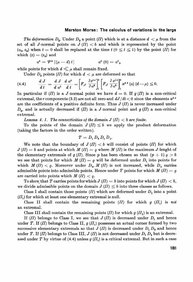
The deformation D3. Under D3 a point (77) which is at a distance d < ju, from the set of all J-normal points on J (77) < b and which is represented by the point (a0, z0) when t = 0 shall be replaced at the time t (0 ^ t f£ 1) by the point (77) for which (z) = (z0) and

ak = Wk [(// — d) t] ak (0) = ak0

while points for which d <|C ft shall remain fixed. Under D3 points (77) for which d < JLI are deformed so tha t

d J d J d ak

dt d ak d t

In particular if (77) is a J-normal point we have d = 0. If g (77) is a non-critical extremal, the r components (3.2) are not all zero and dJ jdt < 0 since the elements ah k

are the coefficients of a positive definite form. Thus J (77) is never increased under D3, and is actually decreased if (77) is a J-normal point and g (77) a non-critical extremal.

Lemma 4. 1. The connectivities of the domain J (77) < b are finite. To the points of the domain J (77) ^ b we apply the product deformation

(taking the factors in the order written).

T = D1 D2 Dx D3.

We note that the boundary of J (77) < b will consist of points (77) for which J (77) = b and points at which M (77) = Q where M (77) is the maximum J-lenght of the elementary extremals of g (II). Since p has been chosen so tha t (p + 1) Q > b we see that points for which M (77) = Q will be deformed under Dx into points for which M (77) < Q. Moreover under D2, M (77) is not increased, while 7)3 carries admissible points into admissible points. Hence under T points for which M (77) = Q are carried into points which M (77) < Q.

To show, that T carries points for which J (77) = b into points for which J (77) < b, we divide admissible points on the domain J (77) ^ 6 into three classes as follows.

Class I shall contain those points (77) which are deformed under 7)1 into a point (/T^ for which at least one elementary extremal is null.

Class I I shall contain the remaining points (77) for which g (Il\) is not an extremal.

Class I I I shall contain the remaining points (77) for which g (771) is an extremal. If (77) belongs to Class I, we see that J (77) is decreased under Dt and hence

under T. If (77) belongs to Class I I , g (7/j) possesses an actual corner formed by two successive elementary extremals so that J (77) is decreased under Dx D2 and hence under T. If (77) belongs to Class I I I , J (77) is not decreased under D± D2 but is decre­ased under T by virtue of (4.4) unless g (T/j) is a critical extremal. But in such a case

181

Grosse Vorträge

J (77J < b since b is an ordinary value of J . Thus under T the domain J (77) < 6 is deformed on itself into a subdomain Z whose boundary is distinct from that of J (77) < b.

Let K be a subcomplex of the product complex 77 that contains all of the points of Z and is so finely subdivided as to consist wholly of points on J (77) < b. We see that any cycle on J (77) < b is homologous to a cycle on K so tha t the connectivities of J (77) < b must be finite. The lemma is accordingly proved.

By a critical value of J we mean a value which J assumes on a critical extremal. We can now prove the following theorem. Theorem 4.1. If a and b (a <b) are two ordinary values of J between which there

are no critical values of J, the connectivities of the domains J (77) < a and J (77) < b will be equal.

The analysis in the preceding proof shows tha t the application of the product deformation Tn to the domain J (77) < b for a sufficiently large power n will deform J (77) < 6 on itself into a subdomain on J (77) < a. The theorem follows readily.

5. The connectivities of the restricted domain J <b. Let kj be a /-complex on the functional domain Ü of § 2 represented by means of the product complex cô x t of an auxiliary /-complex cô and the line segment 0 ^ t ^ 1. If kó is composed of restricted curves on which the J-length of the curves from their initial points to the image of a point Q on Cj x t varies continuously with Q, kj will be called a restricted j-complex. Employing restricted complexes and cycles only, one can now define the connectivi­ties of Q formally as before. We term these connectivities the restricted connectivities. We shall prove the following lemma.

Lemma 5.1. The restricted connectivity Ri of the functional domain Q equals the unrestricted connectivity Pt of Q.

Let kj be an unrestricted complex on Q represented by the product Cj x t as in § 2. Let P be a point on Cj and k (P) the corresponding curve of kó. Let p be a positive integer and let k (P) be divided into p + 1 segments of equal variation of t. Let (77) denote the point on 77 determined by the successive ends of these segments of k (P), and let h be any one of these segments. If p is sufficiently large (and we suppose it is), each point of h can be joined to the initial point of h by an elementary extremal X, independently of the curve k (P) of kj under consideration.

We shall now deform k (P) into g (77). Let x represent the time during this de­formation, 0 fg x S. 1. At each time x we suppose h divided into two segments X and X' in the ratio of x to 1 — x with respect to the variation of t on h. For each value of T we now replace the second of these segments of h by itself, while we replace the first X by the elementary extremal ft which joins its end points. We make a point on X which divides X in a given ratio with respect to t, correspond to the point on ft which divides ft in the same ratio with respect to the variation of J, assigning to this

182

Marston Morse: The calculus of variations in the large

point on ft the same value of t as its correspondent on X bears. We denote this de­formation by dv

We need to subject the resulting curves g (77) to a further deformation ô2 which does not change the curves g (77) except in parameterization. To that end we let the point t on g (77) move along g (77) to the point on g (77) which divides g (77) with res­pect to the J-length in the same ratio as t divides the interval (0,1), moving at a constant J-rate along g (77) equal to the J-length of the arc to be traversed. We term the resulting parameterization a J-parameterization. In it the parameter t runs from 0 to 1 and is proportional to the J-length of the arc preceding the point t.

We denote the product deformation ôx ô2 by Av. Under Ap the curve k (P) is carried into a curve g (77) with a J-parameterization.

If we associate g (77) so parameterized with the point P on Cj it appears that the totality of these curves g (77) forms are stricted complex r (kj) on Û representable by Cj X t.

If kj -> kj-! we see that

(5.1) r (kj) -> r (V i ) -

If kj is a cycle on Q, we see then that r (kj) will be a restricted /-cycle homologous to kj on ß . I t follows tha t Pi <̂ Rt. In particular Ri must be infinite with P t .

To show that Pt = Rt we have merely to show tha t a restricted cycle zó on Ü which bounds an unrestricted complex zJ+1 on Ü necessarily bounds a restricted com­plex as well. To tha t end we suppose tha t

zj+1 -> Zj on Q

If the index p of Ap is sufficiently large, we can apply Ap to zJ+1. We then have

(5.2) r (zJ+1) -> r («,).

But if Zj is deformed under Av through the complex wJ+1 we have (always mod. 2).

(5.3)B wJ+1->Zj + r(Zj),

and hence from (5.2) and (5.3)

Moreover the left complex is a restricted complex since Zj is restricted. Hence Pi = Ri and the lemma is proved.

We shall now prove the following lemma. Lemma 5.2. The restricted connectivities R/ of the restricted domain J <b equal

the connectivities R/' of the subdomain J (77) < 6 of II. The latter connectivities are thus independent of the number of vertices (p + 2) of their points (77), provided only that (p + 1) g > b.

183

Grosse Vorträge

Let Cj be a complex on J (77) < 6. The set of broken extremals g (77) determined by points (77) on Cj if given a 'J-parameterization' will afford a restricted complex CjP

onQ represented by the product Cj x t. A restricted complex cj* derived from a com­plex Cj on 77 in this manner will be called a p-fold complex.

We see that cdv will be a cycle on Q if and only if c5 is a cycle on 77, and that

CjV will bound among p-fold complexes on J < b if and only if có bounds on J (77) < 6. The connectivities of the domain J < 6 on ß defined in terms of p-fold complexes for a fixed p will then equal the connectivities R" of J (77) < b.

But on the other hand any restricted /-cycle of Q on J < 6 can be deformed under Ap among restricted /-complexes of Ü on J < b into a /-complex c/37 on J < 6, so that Ri fg 72/'. To prove that R/ = R/' one has merely to prove, as under the preceding lemma, tha t a p-fold cycle kj on J < b bounds a restricted complex on J <b only if it bounds a p-fold complex on J < b.

To that end we suppose that kj bounds a restricted complex kJ+1 on J < b. As in (5.2) we have

r (^.+1) -> r (kj).

But the vertices of each curve g (77) of r (kj) lie on the curve g (77J from which it is deformed under Ap. We can deform g (TTJ into g (77) deforming ^ into r (kj) through a complex wJ+1 by letting each vertex of (77J move along g (77J to the corresponding vertex of g (77) at a J-rate equal to the J-length of the arc of g (77) to be traversed. We then have

r (kJ+1) + wJ+1 -* kj

and the left hand complex is a p-fold complex. Thus kj bounds a p-fold complex on J < 6 if it bounds a restricted complex on

J <b. Hence R/ = R/' and the lemma is proved. The preceding lemma taken with Theorem 4.1 now gives us the following. Theorem 5.1. If a and b, a <b, are any two ordinary values of J between which

there are no critical values of J, the restricted connectivities of the functional domains J <b and J < a are equal.

6. Spannable and critical cycles. Any two points in our Riemannian space R will be said to possess a J-distance equal to the inferior limit of the J-lengths of restricted curves joining the two points. We see that this J-distance between the two points varies continuously with the points.

We shall now define the J-distance between two curves gx and g2 of class D1. To that end let us regard points on g± and g2 as corresponding if they divide gx

and g2 in the same ratio with respect to the J-lengths of their arcs. We now define the J-distance d (gl9 g2) between gx and g2 as the maximum of the J-distances between

184

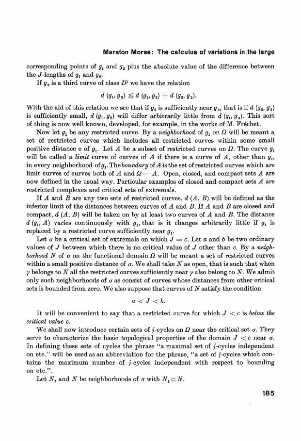
Marston Morse: The calculus of variations in the large

corresponding points of gx and g2 plus the absolute value of the difference between the J-lengths of gx and g2.

If g 3 is a third curve of class D1 we have the relation

d (gl9 g3) ^ d (gl9 g2) + d (g2, g3).

With the aid of this relation we see that if g2 is sufficiently near gs, that is if d (g2, g3) is sufficiently small, d (gx, g2) will differ arbitrarily little from d (gl9 g3). This sort of thing is now well known, developed, for example, in the works of M. Fréchet.

Now let gx be any restricted curve. By a neighborhood of g1 on Q will be meant a set of restricted curves which includes all restricted curves within some small positive distance e of ^ . Let J. be a subset of restricted curves on Q. The curve g1

will be called a limit curve of curves of A if there is a curve of A, other than gl9

in every neighborhood of gx. The boundary of A is the set of restricted curves which are limit curves of curves both of A and Q — A. Open, closed, and compact sets A are now defined in the usual way. Particular examples of closed and compact sets A are restricted complexes and critical sets of extremals.

If A and B are any two sets of restricted curves, d (A, B) will be defined as the inferior limit of the distances between curves of A and B. If A and B are closed and compact, d (A, B) will be taken on by at least two curves of A and B. The distance d (gl9 A) varies continuously with gl9 that is it changes arbitrarily little if gx is replaced by a restricted curve sufficiently near g±.

Let or be a critical set of extremals on which J = c. Let a and b be two ordinary values of J between which there is no critical value of J other than c. By a neigh­borhood N of a on the functional domain Ü will be meant a set of restricted curves within a small positive distance of a. We shall take N as open, that is such tha t when y belongs to N all the restricted curves sufficiently near y also belong to N. We admit only such neighborhoods of a as consist of curves whose distances from other critical sets is bounded from zero. We also suppose that curves of N satisfy the condition

a < J < b.

I t will be convenient to say that a restricted curve for which J < c is below the critical value c.

We shall now introduce certain sets of /-cycles on Ü near the critical set a. They serve to characterize the basic topological properties of the domain J < c near a. In defining these sets of cycles the phrase "a maximal set of /-cycles independent on etc." will be used as an abbreviation for the phrase, "a set of /-cycles which con­tains the maximum number of /-cycles independent with respect to bounding on etc.".

Let Nx and N be neighborhoods of a with N±czN.

185

Grosse Vorträge

A /-cycle on Nt below c, bounding on Nt but not bounding on N below c, will be called a spannable cycle corresponding to N and Nt (written corr. N NJ. A j-cycle on N± independent on N of /-cycles below c will be called a critical cycle corr. N Nt. For suitable choices of N and Nt we shall see that the following maximal sets of /-cycles exist (are finite).

The set (a)Jm A maximal set of spannable j-cycles corr. N Nl9 independent on N below c.

The set (c)j. A maximal set of critical j-cycles corr. N Nl9 independent on N of j-cycles on N below c.

We now state a basic theorem. Theorem 6. There exists a fixed neighborhood N* of a and corresponding to each

neighborhood N czN* a neighborhood M (N) a N with the following property. Corresponding to any two choices of the pair of neighborhoods N Nx satisfying the

conditions

(6.1) NcN* NxcM{N)

there exist common maximal sets of spannable or critical k-cycles on any arbitrarily small neighborhood of a.

We shall term three neighborhoods NQNN-L admissible if N Nx satisfy (6.1), and N0N also satisfy (6.1) as an instance of N N1 in (6.1). We admit only such pairs of neighborhoods N N± as belong to an admissible triple. We abbreviate the phrase "corresponding to an admissible pair of neighborhoods N N^' by writing it in the form corr. N Nv

7. Classification of cycles of Ü on J < b. Suppose now that a is the set of all criti­cal extremals at which J = c. A spannable A-cycle corr. N N± which does not bound below c will be termed newly bounding corr. N Nl9 and a spannable cycle which bounds below c a linkable cycle corr. N Nv We see that a maximal set (a)k of spannable A-cycles can be made up of a maximal set (l)k of linkable A-cycles independent on N below c, together with a maximal set (b)k of newly bounding A-eycles independent on N below c of linkable A-cycles.

Let lk^t be any linkable (k — 1) -cycle corr. N Nt. We have

(7.0) V ' -* t - i below c

where Xk" is a ^-complex on Q. But we also have

(7.1) V - > 4 - i on N,

where Xk is again a complex on Q. We now introduce the fe-cycle

(7-2) K + h" = h We say that Xh links lk+1 corr. N N1.

186

Marston Morse: The calculus of variations in the large

A set of k cycles (X)k linking the respective (k — 1)-cycles of a maximal set of linkable (k— l)-cycles corr. N N1 will be called a maximal set of linking k-cycles corr. N Nv

A k-cjcle below c independent below c of the newly bounding ^-cycles corr. N Nx

will be called an invariant k-cycie corr. N Nx. By a maximal set (i)k of invariant ^-cycles corr. N N1 is meant a set 01 such A-cycles, independent below c of newly bounding A-cycles corr. N N±.

We now state the basic theorem. Theorem 7.1. A maximal set of restricted k-cycles on J <b is afforded by maximal

sets of linking, critical, and invariant k-cycles corr. N Nv

We also have the following. In case c is an absolute minimum of J, and b separates c from the other critical values

of J, then a maximal set of restricted k-cycles on J <b is afforded by the critical k-cycles corr. N Nv

8. The existence of critical extremals. Relative to the critical value c we shall call a A-cycle a new A-cycle if it is independent on J < b of cycles on J < a. We shall consider maximal sets of new ^-cycles independent on J < 6 of ^-cycles on J < a. By virtue of Theorem 7.1 such a maximal set will be afforded by a maximal set of critical ^-cycles corr. N N± and Unking A-eycles corr. N N Nv

Relative to the critical value c we shall call a A-cycle newly bounding if it lies on J < a, is bounding on J < 6 , but non-bounding on J<a. We shall consider maximal sets of newly bounding fc-cycles independent on J < a but bounding on J < 6. According to Theorem 7.1 such a maximal set will be afforded by a maximal set of newly bounding ^-cycles corr. N Nv

The number of cycles in a maximal set of new A-cycles depends upon more than the neighborhood of o. The same is true of the number of cycles in a maximal set of newly bounding (k — 1)-cycles. I t is a remarkable fact however tha t the sum of the two preceding numbers depends only upon the nature of J neighboring G, in fact is the number of cycles in a maximal set of critical ^-cycles, and a maximal set of spannable (k— 1)-cycles. Moreover this sum is additive for the separate critical sets. We are thus led to the following definition.

The Ath type number M of a critical set a shall be defined as the number of cycles in the corresponding maximal sets of critical k-cycles and spannable (k — l)-cycles corr. NNV

The kth type number of a sum of critical sets will be defined as the sum of the respective type numbers of the component sets.

We state the following principal theorem.

Theorem 8. Let N0N1 ... be the type number sums for all critical sets of extremals,

187

Grosse Vorträge

and let P0 Px ... be the connectivities of the function space Ü. If the numbers N{ are finite they satisfy the infinite set of inequalities.

,A* N0-N1^P0-Pl ( ) N0~N1-N2^P0-Pl + P2.

If all of the integers Nx are finite for i < r + 1 the first r + 1 relations in (A) still hold.

Further details and extensions will be given in the Colloquiom Lectures by the author.

1. Tonelli, Fondamenti di Calcolo delle Variazioni. * 2. Signorini, Rendiconti del Circolo Matematico di Palermo, voi. 33 (1912) pp. 187—193. Here

broken geodesies are used in the quest for a minimum. 3. Birhhoff, Dynamical Systems. American Mathematical Society Colloquium Publications,

vol. 9. Birkhoff's minimum and minimax methods are developed here. 4. MM. Lusternik et Schnirelmann, Topological Methods in Variational Problems. Research

Insti tute of Mathematics and Mechanics Gosizdat Moscow (1930). Here a topological theory of critical points of functions is developed. Specific results in the calculus of variations are confined mostly to the problem of the closed geodesic on the image of the 2-sphere.

5. Morse, Transactions of the American Mathematical Society, vol. 27 (1925), pp. 345—396. 6. Morse, Ibid vol. 30 (1928), pp. 213—274. 7. Morse, Ibid vol. 31 (1929), pp. 379—404. 8. Morse, Ibid vol. 32 (1930), pp. 599—631. 9. Morse, Ibid vol. 33 (1931), pp . 72—91. 10. Morse, Proceedings of the National Academy of Sciences, vol. 15 (1929), pp. 856—859. Extremal

chords, and periodic extremals. 11. Morse, Annals of Mathematics, vol. 32 (1931), pp. 549—566. 12. Morse, Calculus of Variations. American Mathematical Society Colloquium Publications.

Not yet published. 13. Lefschetz, Topology. American Mathematical Society Colloquium Publications. 14. Eisenhart, Riemannian Geometry. 15. Osgood, Funktion en théorie I I . 16. Ponincaré, Liouville Journal 4th series, vol. 1 (1885) pp. 167—244. The equality in the case

n = 2 was used by Poincaré.

188