Calculus if variations

7/29/2019 Calculus if variations

http://slidepdf.com/reader/full/calculus-if-variations 1/32

A VARIATIONAL METHOD IN IMAGE RECOVERY∗

GILLES AUBERT† AND LUMINITA VESE‡

SIAM J. NUMER. ANAL. c 1997 Society for Industrial and Applied MathematicsVol. 34, No. 5, pp. 1948–1979, October 1997 016

Abstract. This paper is concerned with a classical denoising and deblurring problem in imagerecovery. Our approach is based on a variational method. By using the Legendre–Fenchel transform,we show how the nonquadratic criterion to be minimized can be split into a sequence of half-quadraticproblems easier to solve numerically. First we prove an existence and uniqueness result, and then wedescribe the algorithm for computing the solution and we give a proof of convergence. Finally, wepresent some experimental results for synthetic and real images.

Key words. image processing, Legendre–Fenchel transform, partial differential equations, cal-culus of variations

AMS subject classifications. 35J, 49J, 65N

PII. S003614299529230X

1. Introduction. An important problem in image analysis is the reconstruc-

tion of an original image f describing a real scene from an observed image p. Thetransformation (or degradation) connecting f to p is in general the result of two phe-nomena. The first phenomenon is deterministic and is related to the mode of imageacquisition (for example, the computation of integral projections in tomography) or topossible defects of the imaging system (blur created by a wrong lens adjustement, bya movement,. . .). The second phenomenon is random: the noise inherent degradationin any signal transmission. Suppose that the noise denoted by η is white, Gaussian,and additive.

The simplest model accounting for both blur and noise is the linear degradationmodel: we suppose that f is connected to p by an equation of the form

(1.1) p = Rf + η,

where R is a linear operator. (We remain, for the moment, intentionally vague onthe exact significance of (1.1)—in particular, on the space on which this equation isdefined.)

The reconstruction problem of f can be identified, in that way, with an inverseproblem: find f , from (1.1). In general, this problem is ill-posed in the sense of Hadamard. The information provided by p and the model (1.1) is not sufficient toensure the existence, uniqueness, and stability of a solution f .

It is therefore necessary to regularize the problem by adding an a priori constrainton the solution. The most classical and frequent approach in image reconstructionis a stochastic approach based, in the framework of Bayesian estimation, on the useof maximum a posteriori (MAP) estimation. Supposing that f is a Markov field(which constitutes an a priori constraint), then the MAP criterion identifies with aminimization problem in which the energy J depends on the image f and on the

gradient. We are not going into the details of this approach; instead, we refer the∗Received by the editors September 22, 1995; accepted for publication (in revised form) February

6,1996.http://www.siam.org/journals/sinum/34-5/29230.html

†Laboratoire de Mathematiques, Universite de Nice, Parc Valrose, BP 71, F 06108 Nice, Cedex02, France ([email protected]).

‡Laboratoire de Mathematiques, Universite de Nice, Parc Valrose, BP 71, F 06108 Nice, Cedex02, France ([email protected]).

1948



A VARIATIONAL METHOD IN IMAGE RECOVERY 1949

reader to the original article of Geman and Geman [13] or, for a clear and syntheticexposition, to the work of Charbonnier [4].

Our purpose being to study the problem of image reconstruction via the calculusof variations and partial differential equations, we do not develop a new model here.

We will study for a continuous image the model described by Geman and Geman fora numerical image (or a slight modification of this).

In section 2, we will present more precisely the minimization problem studiedhere, as well as the assumptions to impose on the model. These will be imposed bythe requirements that we wish to obtain on the results. In section 3 we will show byusing the Fenchel–Legendre transform how we can introduce in the energy J (possiblynonconvex) a dual variable b allowing us to reduce the minimization of J to a sequenceof quadratic minimization problems. In section 4 we will study the problem of theexistence and uniqueness of a solution f . The obtained results are based on a singularperturbation result of Temam [12]. Moreover, we note the analogy of our problemwith the one of minimal surfaces studied by Temam in [12] and [26]. In section 5 wewill describe the algorithm in continuous variables for computing the solution, as wellas a convergence proof. Finally, in sections 6 and 7, we develop the numerical analysis

of the approximated problem, and we try to validate the model by presenting someexamples with synthetic or real images.

2. Description of the model. Assumptions. In continuous variables the ob-served image p and the reconstructed image f can be represented by functions of Ω ⊂R2 → R which associate with the pixel (x, y) ∈ R2 its gray level p(x, y) or f (x, y); Ω is

the support of the image (a rectangle in general). The gray levels being in finite num-ber, we can suppose that the observation p(x, y) verifies 0 ≤ p(x, y) ≤ 1∀(x, y) ∈ Ω.

The stochastic model proposed by Geman and Geman for image reconstructionleads us, as we pointed out in the introduction, to search for a solution among theminima of the energy

J α(f ) = Ω

( p(x, y)

−(Rf )(x, y))2dxdy + α

Ω

φ(

|Df (x, y)

|)dxdy.(2.1)

R is a linear operator of L2(Ω) → L2(Ω), and the first integral represents an attachedterm on the data. The function φ : R+ → R

+ is to be defined and symbolizes theregularization term (hence, a constraint on the solution). In [13], Geman and Gemanhave added a regularization term of the form

Ω

φ∂f

∂x

+ φ

∂f

∂y

dxdy,

corresponding (for numerical images) to a regularization on lines and columns. Thisterm, unlike ours, is not invariant under rotation. The number α ∈ R+ is a parameterwhich allows us to balance the influence of each integral in the energy J α(f ). If α = 0,

J α(f ) is

J 0(f ) =

Ω

( p(x, y) − (Rf )(x, y))2dxdy,

and so the energy is reduced only to the attached term on the data, and the problem

inf f

J 0(f )(2.2)



1950 GILLES AUBERT AND LUMINITA VESE

corresponds to the least-squares method associated with the equation (1.1). Formally,every solution of (2.2) verifies the equation

R∗ p = R∗Rf,(2.3)

where we have denoted by R∗ the adjoint operator of R. Generally, (2.3) is an ill-posedproblem: R∗R is not always invertible or the problem (2.3) is often unstable.

To overcome this difficulty, we either look for a solution in a smaller set (wherewe have some compactness), or we add a regularization term to the attached term onthe data. This method, which is due to Tikhonov [27], is the one we use here, andthe additional term is represented in (2.1) by

Ω

φ(|Df (x, y)|)dxdy. It now remainsto find some appropriate conditions on the function φ in order to satisfy the followingprinciple of image analysis:

The reconstructed image must be formed by homogeneous regions,(2.4)

separated by sharp edges.

The model must, therefore, diffuse within the regions where the variations of graylevels are weak, and otherwise, it must preserve the boundaries of these regions; thatis, it must respect the strong variations of gray levels.

So, supposing that the integrals in J α(f ) have made sense, then any function real-izing the minima of J α must formally verify (for instance, in the sense of distribution)the Euler equation J

α(f ) = 0 or

−α

2divφ

(|Df |)|Df | Df

+ R∗Rf = R∗ p.(2.5)

Writing (2.5) in a nonconservative form, we will obtain some sufficient assump-tions on φ, in order to respect, as much as possible, the principle (2.4). To do this,

for each point (x, y) where

|Df (x, y)

| = 0, let the vectors T (x, y) =

Df (x,y)|Df (x,y)| in the

gradient direction, and ξ (x, y) in the orthogonal direction to T (x, y). With the usualnotations f x, f y, f xx, . . . for the first and second partial derivatives of f , and by for-mally developing the divergence operator, (2.5) can be written as

−α

2

φ

(|Df |)|Df |

f ξξ − α

2φ

(|Df |)f TT + R∗Rf = R∗ p,(2.6)

where we have denoted by f ξξ and f TT the second derivatives of f in the directionsξ (x, y) and T (x, y), respectively:

f ξξ =1

| Df |2 (f 2xf yy + f 2y f xx − 2f xf yf xy),

f TT =

1

| Df |2 (f

2

xf xx + f

2

y f yy + 2f xf yf xy).

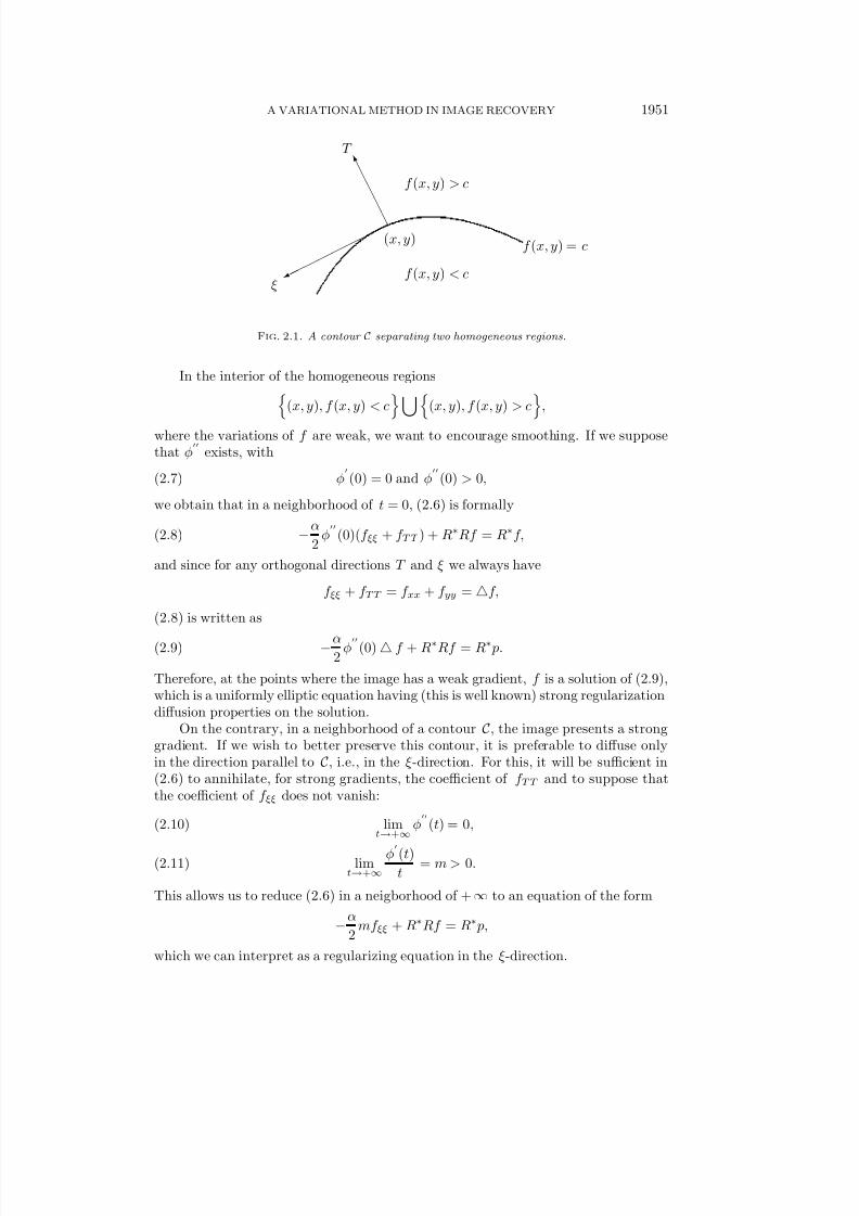
If f is regular (at least continuous), we can interpret the principle (2.4) in the followingmanner (as shown in Figure 2.1): locally, we represent a contour C separating twohomogeneous regions of the image, by a level curve of f : C = (x, y); f (x, y) = c .In this case, the vector T (x, y) is normal to C at (x, y) ∈ C, and the expressionf ξξ(x,y)

|Df (x,y)|=div( Df (x,y)|Df (x,y)|

) represents the curvature of C at this point.




e e e e e u

¨ ¨ ¨ ¨ ¨ ¨ ¨ ¨ %

f (x, y) = c

f (x, y) < c

f (x, y) > c

(x, y)

T

ξ

FIG. 2.1. A contour C separating two homogeneous regions.

In the interior of the homogeneous regions

(x, y), f (x, y) < c(x, y), f (x, y) > c,

where the variations of f are weak, we want to encourage smoothing. If we supposethat φ

exists, with

φ

(0) = 0 and φ

(0) > 0,(2.7)

we obtain that in a neighborhood of t = 0, (2.6) is formally

−α

2φ

(0)(f ξξ + f TT ) + R∗Rf = R∗f,(2.8)

and since for any orthogonal directions T and ξ we always have

f ξξ + f TT = f xx + f yy = f,

(2.8) is written as

−α2

φ

(0) f + R∗Rf = R∗ p.(2.9)

Therefore, at the points where the image has a weak gradient, f is a solution of (2.9),which is a uniformly elliptic equation having (this is well known) strong regularizationdiffusion properties on the solution.

On the contrary, in a neighborhood of a contour C, the image presents a stronggradient. If we wish to better preserve this contour, it is preferable to diffuse onlyin the direction parallel to C, i.e., in the ξ -direction. For this, it will be sufficient in(2.6) to annihilate, for strong gradients, the coefficient of f TT and to suppose thatthe coefficient of f ξξ does not vanish:

limt→+∞

φ

(t) = 0,(2.10)

limt→+∞

φ

(t)t

= m > 0.(2.11)

This allows us to reduce (2.6) in a neigborhood of +∞ to an equation of the form

−α

2mf ξξ + R∗Rf = R∗ p,

which we can interpret as a regularizing equation in the ξ -direction.




But (2.10) and (2.11) are not compatible, and one must make a compromisebetween these two hypotheses; for example, by supposing that φ

(t) and φ

(t)/t bothconverge to zero as t → ∞ but with different speeds. More precisely, we suppose that

(2.12a) limt→+∞

φ

(t) = limt→+∞

φ

(t)t

= 0,

(2.12b) limt→+∞

φ

(t)φ(t)t

= 0,

that is, that φ

converges faster to 0 than φ

(t)/t, which makes preponderant thecoefficient of f ξξ in (2.6).

The preceding assumptions, (2.7) and (2.12), are rather of qualitative type andrepresent a priori the properties that we want to obtain on the solution. But theseare not sufficient to prove that the model is well posed mathematically. To do this,in order to use the direct method of calculus of variations, we suppose that

(2.13) limt→+∞

φ(t) = +∞;

this assumption ensures the boundness of the minimizing sequences of

J α(f ) =

Ω

( p − Rf )2dxdy + α

Ω

φ(|Df |)dxdy.

This growth to infinity must not be too strong because it must not penalize stronggradients (or formation of edges). Hence, we suppose a linear growth to infinity:

(2.14)

There exist constants ai > 0 and bi ≥ 0, i = 1, 2, such that

a1t − b1 ≤ φ(t) ≤ a2t + b2 ∀t ∈ R+,

and then the natural space on which we seek the solution will be

V =

f ∈ L2(Ω), Df ∈ L1(Ω)2

.

Finally, for passing to the limit on the minimizing sequences of (2.1) and to obtainthe uniqueness of a solution, we suppose that

(2.15) t → φ(t) is strictly convex on R+ → R+.

Remark. A better growth condition than (2.14), which doesn’t penalize the for-mation of edges, could be limt→∞ φ(t) = c > 0. In this case, if M denotes a min-imal threshold representing strong gradients, then the contribution of the integral |Df |≥M φ(|Df |)dxdy in the energy is nearly a constant and then the formation of

an edge does not “cost” anything in the energy. But the hypothesis of a horizontalasymptote introduces in general a nonconvexity on φ for t ≥ M , and we know, in thiscase, that the problem is ill-posed and can have no solution. Nevertheless, we have

done some numerical tests with the function φ(t) = t2

1+t2 (which is of this type of potential and verifies (2.7) and (2.12a)). The results obtained are very satisfactory.

To clarify the exposition, we now summarize our assumptions on the potential φ.




Hypotheses for φ.(H1) The function φ : R+ → R

+ is of class C 2, is nondecreasing, and satisfiesφ

(0) = 0 and φ

(0) > 0.(H2) The function φ : R+ → R

+ has the properties

limt→+∞

φ

(t) = limt→+∞

φ

(t)

t= 0 and lim

t→+∞

φ

(t)φ(t)t

= 0.

(H3) There exist constants ai > 0 and bi ≥ 0, i = 1, 2, such that

a1t − b1 ≤ φ(t) ≤ a2t + b2 ∀t ∈ R+.

(H4) The function φ : R+ → R+ is strictly convex.

If it will be necessary to define the function φ on the whole space, we will extendit by parity of R+ to R. Other hypotheses due to the numerical approximation willbe added in the following sections.

Of course, there are many functions φ verifying (H1)–(H4), and no criterion per-mits the choice of a potential more than any other. Charbonnier, in [4], presents many

choices used in image reconstruction as well as a comparative study. Our choice herefor the tests is the function φ(t) =

√ 1 + t2 which verifies (H1)–(H4) and, moreover,

has a simple and geometric interpretation (the problem of minimal surfaces).This paper is closely related to the works of Malik and Perona [20], Catt e et al. [2],

Rudin and Osher [22], and Chambolle and Lions [3]. Our approach is more orientedtowards the techniques of the calculus of variations than those of PDEs. This papercompletes, in a theoretical point of view, a preceding work concerning tomographicreconstruction [5], [6]. See also [1], [14], [29].

3. Auxiliary variable. Half-quadratic reduction. Before proving the exis-tence of a solution, we will show in this section how we can associate an auxiliaryvariable (or dual) with the image f and how the regularization term in the energy(2.1) can be represented by the infimum of quadratic functions. We recall that the

energy J α(f ) is

(3.1) J α(f ) =

Ω

( p − Rf )2dxdy + α

Ω

φ(|Df |)dxdy,

the regularization term being

(3.2) Lφ(f ) =

Ω

φ(|Df |)dxdy.

To develop this idea, we use the Fenchel–Legendre transform (see Rockafellar [21]or Ekeland and Temam [12]). We recall that if l(ξ ) is a convex function of RN into R,then its Fenchel–Legendre transform (or polar) is the convex function l∗(ξ ∗) definedby

l∗

(ξ ∗

) = supξ∈RN (ξ · ξ ∗

− l(ξ ))

(ξ ·ξ ∗ is the usual scalar product). This definition can be extended, without difficulty,to infinite-dimensional spaces. Let Ω be an open set of RN and l a convex continuousfunction of RN → R, and for u ∈ Lγ (Ω)N , let the functional

L(u) =

Ω

l(u(x))dx.




Then the polar of L, denoted L∗, is defined on Lγ

(Ω)N , the dual space of Lγ (Ω)N ,where 1

γ + 1

γ = 1, by

L∗(u∗) = supu∈Lγ

(Ω)N

Ω

u(x)u∗(x)− Ω

l(u(x))dx.

If, in addition, l is nonnegative or if l verifies an inequality of the type l(ξ ) ≥ a(x) −b · |ξ |η

RN , with a(x) ∈ L1(Ω), b ≥ 0, and η ∈ [1, ∞), and if there exists u0 ∈ L∞(Ω)N

such that L(u0) < ∞, then we can prove (see Ekeland and Temam [12, Chap. IX])that L∗(u∗) is written as

L∗(u∗) =

Ω

l∗(u∗(x))dx.

Of course, we can reiterate the process and define

L∗∗(u) =

Ω

l∗∗(u(x))dx.

Since l is convex, we have l(ξ ) = l∗∗(ξ ) and then L∗∗(u) = L(u).We use this notion of polarity in our problem with N = 2, γ = γ

= 2. Let, forξ, ξ ∗ ∈ R2,

l(ξ ) =|ξ |2

2− φ(|ξ |),(3.3)

ψ(ξ ∗) = l∗(ξ ∗) − |ξ ∗|22

,(3.4)

as well as the functionals defined on L2(Ω)2 by

Φ(u) =

Ω

φ(|u(x, y)|)dxdy

=

Ω

|u(x, y)|22

− l(u(x, y))

dxdy

,(3.5)

Ψ(b) = Ω

ψ(b(x, y))dxdy.(3.6)

The following theorem proves that Φ and Ψ are dual in a certain sense.THEOREM 3.1. If φ (extended by parity on R) verifies the following hypotheses:(H3) there exist constants ai > 0 and bi ≥ 0, i = 1, 2, such that

a1|t| − b1 ≤ φ(t) ≤ a2|t| + b2 ∀ t ∈ R;

(H5) the function t → t2

2 − φ(t) is convex on R,then

Φ(u) = inf b∈L2(Ω)2

Ω

|u − b|22

+ ψ(b)

dxdy,(3.7)

Ψ(b) = supu∈L2(Ω)2

Ω

− |u − b|2

2+ φ(|u|)

dxdy.(3.8)

Proof . We prove (3.7). Let ρ(u) be the value of the infimum in (3.7):

ρ(u) =

Ω

|u|22

dxdy + inf b

Ω

|b|22

− b · u + ψ(b)

dxdy.




This can be also written, with (3.4), as

ρ(u) =

Ω

|u|22

dxdy + inf b

Ω

|b|22

− b · u + l∗(b) − |b|22

dxdy

= Ω

|u|2

2dxdy − sup

b

Ω

b · u − l∗(b)

dxdy.

Then (by Ekeland and Temam [12]),

ρ(u) =

Ω

|u|22

dxdy − Ω

l∗∗(u)dxdy.

From (H5) we have that l∗∗(ξ ) = l(ξ ) ∀ξ ∈ R2; hence

ρ(u) =

Ω

|u|22

dxdy − Ω

l(u)dxdy = Φ(u).

Equation (3.8) can be proved in the same manner.

We have remarked that we must seek a solution on the space

V =

f ∈ L2(Ω), Df ∈ L1(Ω)2

.

But in order to use the duality, we will look for a solution f on the space H 1(Ω).By using the relation (3.7), J α(f ) is written, for f ∈ H 1(Ω), as

J α(f ) =

Ω

( p − Rf )2dxdy + α inf b∈L2(Ω)2

Ω

|Df − b|22

+ ψ(b)

dxdy,

and then

inf f ∈H 1(Ω)

J α(f ) = inf f ∈H 1(Ω)

inf b∈L2(Ω)2

Ω

( p−Rf )2dxdy +α

Ω

|Df − b|22

+ψ(b)

dxdy

.

Because we can always invert the infinima, we get

inf f ∈H 1(Ω)

J α(f ) = inf b∈L2(Ω)2

α

Ω

ψ(b)dxdy + inf f ∈H 1(Ω)

Ω

( p−Rf )2+α

|Df − b|22

dxdy

and the method is now clear: we fix b ∈ L2(Ω)2 and we solve the problem

(P b) inf f ∈H 1(Ω)

Ω

( p − Rf )2 + α

|Df − b|22

dxdy

.

If R satisfies some appropriate assumptions, then (P b) has a unique solution, whichis, formally, a solution of the Euler equation:

(3.9)

−α

2 f b + R∗Rf = R∗ p

−α

2

divb, in

D

(Ω),

∂f b∂η = 0, on ∂ Ω.

We have then, for all v ∈ H 1(Ω) and for all b,

(3.10)

Ω

( p − Rf b)2 +

α

2|Df b − b|2

dxdy ≤

Ω

( p − Rv)2 + α

|Dv − b|22

dxdy.




By adding Ω

ψ(b)dxdy on each side of (3.10), and by passing to the infimum in b, weget, for all v ∈ H 1(Ω),

inf b∈L2(Ω)2

Ω( p − Rf b)2 +

α

2|Df b − b|2 + αψ(b)dxdy(3.11)

≤ Ω

( p − Rv)2 + αφ(|Dv|)

dxdy.

Denoting

T (b) =

Ω

( p − Rf b)2 +

α

2|Df b − b|2 + αψ(b)

dxdy,

it is then sufficient, in order to prove that our algorithm allows us to solve the initialreconstruction problem, to obtain the existence of b0 ∈ L2(Ω)2 such that

T (b0) = inf b∈L2(Ω)2

T (b) with(3.12)

T (b0) = Ω( p

−Rf b0)2 + αφ(

|Df b0

|)dxdy = J α(f b0).

We will then deduce, with (3.11), that

(3.13) J α(f b0) ≤ J α(v) ∀v ∈ H 1(Ω).

At this stage we must precisely formulate the mathematical assumptions in order toensure the existence and uniqueness of a solution. There is a problem due to the factthat we work with sets constructed from the nonreflexive Banach space L1(Ω).

4. Existence and uniqueness of a solution. To simplify, we will suppose thatR = I on L2(Ω) (which corresponds to a denoising problem), and we will indicatein Appendix B the minor modifications to add if R = I . We also suppose that theweighting parameter α is equal to 1, which does not modify the theoretical study of the problem (its presence and adjustment are fundamental in the applications). The

studied functional is therefore

(4.1) J (f ) =

Ω

( p − f )2dxdy +

Ω

φ(|Df |)dxdy.

The basic assumptions that we will suppose to be verified in this section are as follows:(4.2) p ∈ L∞(Ω) and 0 ≤ p(x, y) ≤ 1 a.e. (x, y) ∈ Ω,(4.3) φ : R → R is even, of class C 2, nondecreasing on R+, and there exist constants

ai > 0, bi ≥ 0, i = 1, 2, such that a1|t| − b1 ≤ φ(t) ≤ a2|t| + b2∀t ∈ R,(4.4) 0 < φ

(t) < 1∀t ∈ R.

Remark. From (4.4), the functions φ(t) and t2

2 − φ(t) are strictly convex (i.e., thehypothesis (H5), which is strengthened).

Thanks to (4.4), with the notations of the preceding section, J (f ) can be written,for f

∈H 1(Ω), as

J (f ) = inf b∈L2(Ω)2

Ω

( p − f )2 +

Ω

|b − Df |22

+ ψ(b)

dxdy.

PROPOSITION 4.1. For fixed b in L2(Ω)2 and for p satisfying (4.2), the problem

(4.5) inf f ∈H 1(Ω)

Ω

( p − f )2 +

|b − Df |22

dxdy




has a unique solution f b ∈ H 1(Ω) verifying the Euler equation

(4.6) − f b + 2f b = 2 p − divb in D

(Ω).

Proof . The functional

J b(f ) =

Ω

( p − f )2 +

|b − Df |22

dxdy

being continuous, strictly convex, and coercive on H 1(Ω), then, by the classical theoryof calculus of variations, there exists a unique f b ∈ H 1(Ω) such that

(4.7) J b(f b) ≤ J b(f ) ∀f ∈ H 1(Ω),

which is equivalent to

2

Ω

(f b − p)fdxdy +

Ω

(Df b − b) · Dfdxdy = 0 ∀f ∈ H 1(Ω).

Then we obtain (4.6), choosing f ∈ D(Ω).Remark. For the moment, we will not include in (4.6) the usual condition on the

boundary ∂ Ω of Ω: ∂f ∂η

(x) = 0, the H 1-regularity of f b being insufficient to define thevalue on the boundary of the normal derivative.

Hence, we have for all f ∈ H 1(Ω) and fixed b

(4.8)

Ω

(f b − p)2dxdy +

Ω

|b − Df b|22

dxdy ≤ Ω

(f − p)2dxdy +

Ω

|b − Df |22

dxdy,

and by adding ψ(b) on each side of (4.8) and taking the infimum in b, for all f ∈ H 1(Ω),we obtain

inf b∈L2(Ω)2 Ω

(f b − p)2

+ |b

−Df b

|2

2 + ψ(b)

dxdy(4.9)

≤ Ω

(( p − Rf )2 + φ(|Df |))dxdy = J (f ).

We recall that

T (b) =

Ω

(f b − p)2 +

1

2|b − Df b|2 + ψ(b)

dxdy.

Now we must prove that the problem inf b∈L2(Ω)2 T (b) has a solution b0, which willinvolve the existence of a function f 0 solution of the initial problem

J (f 0) ≤ J (f ) ∀f ∈ V .

First, we will state some properties of the dual function ψ.LEMMA 4.2. If φ verifies (4.3) and (4.4), then the function ψ defined by (3.4) has

the following properties:(4.10) ξ ∗ → ψ(ξ ∗) is strictly convex,(4.11) there exist constants a

i > 0 and b

i ≥ 0 such that

a

1|ξ ∗| − b

1 ≤ ψ(ξ ∗) ≤ a

2|ξ ∗| + b

2 ∀ξ ∗ ∈ R2.




Proof . We recall the definition of ψ(ξ ∗). If l(ξ ) denotes the strictly convex function(from (4.4))

l(ξ ) =|ξ |2

2 −φ(

|ξ

|),

then ψ(ξ ∗) is defined by

ψ(ξ ∗) = l∗(ξ ∗) − |ξ ∗|22

(l∗ denotes the Fenchel–Legendre transform of l).We prove (4.11):

ψ(ξ ∗) = supξ

ξ ∗ · ξ − l(ξ )

− |ξ ∗|2

2

= supt≥0

sup|ξ|=t

ξ ∗ · ξ − |ξ |2

2+ φ(| ξ |)

− |ξ ∗|2

2

= supt≥0

t|ξ ∗| − t

2

2+ φ(t)

− |ξ ∗

|2

2,

and since φ is even,

ψ(ξ ∗) = supt∈R

t|ξ ∗| − t2

2+ φ(t)

− |ξ ∗|2

2.

Hence, with (4.3), we have

−b1 − |ξ ∗|22

+ supt∈R

a1|t| + |ξ ∗|t − t2

2

≤ ψ(ξ ∗)(4.12)

≤ b2 − | ξ ∗ |22

+ supt∈R

a2|t| + |ξ ∗|t − t2

2

.

The supremum in the right-hand side of (4.12) is achieved for t = a2 + |ξ ∗|, and itsvalue is 1

2(a2 + |ξ ∗|)2; hence, with (4.12),

ψ(ξ ∗) ≤ b2 − |ξ ∗|22

+1

2(a2 + |ξ ∗|)2 = b2 +

1

2a22 + a2 | ξ ∗|,

from which we obtain the second inequality of (4.11), with a

2 = a2 and b

2 = b2 + 12

a22.The first inequality of (4.11) can be proved in the same way. The proof of (4.10)follows from (4.4) and by a classical argument of convex analysis. From (4.4), wehave that the function ξ → l(ξ ) is strictly convex; hence, l∗(ξ ∗) is of class C 2 (byRockfellar [21], Dacorogna [10]) and

∇ψ(ξ ∗) =

∇l∗(ξ ∗)

−ξ ∗,

∇2ψ(ξ ∗) = ∇2l∗(ξ ∗) − I.

Moreover, since l(ξ ) is strictly convex, ∇l(ξ ) is strictly monotonic and then, foreach ξ ∗ ∈ R

2, there is a unique ξ 0 ∈ R2 such that ξ ∗ = ∇l(ξ 0), or equivalently,

∇l∗(ξ ∗) = ξ 0. Hence, we get

(4.13) ∇ψ(ξ ∗) = ξ 0 − ∇l(ξ 0) = −∇(φ(|ξ |))ξ=ξ0 = −φ

(|ξ 0 |)|ξ 0| ξ 0




and (see Crouzeix [9] for computational details)

(4.14) ∇2ψ(ξ ∗) =∇2l(ξ 0)

−1− I,

which can be also written, from the definition of l(ξ ), as

∇2ψ(ξ ∗) =

I − ∇2(φ(|ξ |))ξ=ξ0

−1− I.

Thanks to (4.4), it is then clear that the matrix ∇2ψ(ξ ∗) is symmetric positive definite;consequently, ψ is strictly convex.

Remark. In Lemma 4.2, ξ 0 is, in fact, the unique point realizing the supremumsupξ(ξ · ξ ∗ − l(ξ )) = l∗(ξ ∗).

Provided with the properties of the function ψ, we can now return to the studyof the problem (4.9):

inf b∈L2(Ω)2

T (b) =

Ω

(f b − p)2 +

|b − Df b|22

+ ψ(b)

dxdy

.

If bn is a minimizing sequence, then it is simple to deduce from (4.8) and (4.11) thatbn and f bn verify the estimates

f bnL2(Ω) ≤ c,

bnL1(Ω)2 ≤ c,

where c is a constant which only depends on the data. But we cannot obtain anH 1(Ω)-estimate for f bn and an L2(Ω)2-estimate for bn, hence we must work on thenonreflexive space L1(Ω) or on Mb(Ω), the space of bounded measures. To over-come this difficulty, we regularize the problem by making a slight modification on thepotential φ. We introduce the function

φε(t) = φ(t) +ε

2t2, ε > 0,

with which we associate

lε(ξ ) =|ξ |2

2− φε(|ξ |),

ψε(ξ ∗) = l∗ε(ξ ) − |ξ |22

.

The function ψε has the same properties as ψ if we modify and replace (4.4) by thefollowing:

(4.4)ε There is ε0, with 0 < ε0 < 1 such that 0 < φ

(t) < 1 − ε0, for all t ∈ R.

The assumption (4.4)ε is not restrictive, because we can always change the weightingparameter in the energy J α(f ), to have (4.4)ε verified.

By proceeding as in Lemma 4.2, it is easy to see, for ε ≤ ε0, that

(4.10)ε ξ ∗ → ψε(ξ ∗) is strictly convex,

(4.11)ε −b1 +a21

2(1 − ε)+

a11 − ε

|ξ ∗| +ε

2(1 − ε)|ξ ∗|2 ≤ ψε(ξ ∗)

≤ b2 +a22

2(1 − ε)+

a21 − ε

|ξ ∗| +ε

2(1 − ε)|ξ ∗|2,




and the regularized problem associated with T (b) is

(4.15) inf b∈L2(Ω)2

T ε(b) =

Ω

(f b − p)2 +

|b − Df b|22

+ ψε(b)

dxdy

,

for which we state the following proposition.PROPOSITION 4.3. Under the assumptions (4.2), (4.3), and (4.4)ε, the problem

(4.15) has a unique solution bε and there exists a constant c, independent of ε, such that

(4.16)

εbε2L2(Ω)2 ≤ c,

εDf bε2L2(Ω)2 ≤ c,

bεL1(Ω)2 ≤ c,f bεL2(Ω) ≤ c.

Proof . The functional T ε(b) is strictly convex since, from (4.6), the map b → f bis affine from L2(Ω) to H 1(Ω) and the function ψε is strictly convex (from (4.10)ε).

Moreover, from (4.11)ε, for each b

∈L2(Ω)2 there are some coefficients a

1 > 0

and b

1 such thatε

2b2L2(Ω)2 + a

1bL1(Ω)2 − b

1 ≤ T ε(b);

hence, for fixed ε, the minimizing sequences bnε from (4.15) are bounded in L2(Ω)2;therefore, there exist bε ∈ L2(Ω)2 and a subsequence denoted also by bnε such that

bnεw

bε in L2(Ω) weak. Since to the strict convexity of T ε, bε is unique, the entiresequence bnε converges to bε, and

T ε(bε) ≤ limn→∞

T ε(bnε ) = inf b

T ε(b) ≤ T ε(b) ∀b ∈ L2(Ω)2;

that is, bε is the unique solution of (4.15):

(4.17) Ω

(f bε − p)2 + |bε − Df bε |

2

2 + ψε(bε) + ε2 |bε|2dxdy

≤ Ω

(f b − p)2 +

|b − Df b|22

+ ψε(b) +ε

2|b|2

dxdy ∀b ∈ L2(Ω)2.

Choosing, for example, b = 0 in (4.17), it is clear that there is a constant c,independent of ε, such that (4.16) is verified.

The following theorem examines the optimality condition satisfied by bε.THEOREM 4.4. The solution bε of the problem (4.15) verifies the optimality con-

dition

(4.18) (1 + ε)bε + Dψε(bε) − Df bε = 0 a.e. (x, y) ∈ Ω.

Proof . To simplify the notations, we denote f ε = f bε ; then let us consider avariation of bε of the form bθ = bε + θq , where θ ∈ R and q ∈ L2(Ω)2. Denotingf θ = f bθ , it is clear, thanks to the linearity of formula (4.6), that

(4.19) f θ = f ε + θh,

where h verifies

(4.20) − h + 2h = −divq in H 1(Ω)

(the dual of H 1(Ω)).




With this remarkT ε(bθ) − T ε(bε)

θ

(4.21) = Ω(2f ε − 2 p + θh)hdxdy +

Ω(2bε − 2Df ε + θ(q − Dh)) · (q − Dh)dxdy

+1

θ

Ω

(ψ(bε + θq ) − ψ(bε))dxdy.

Now, as θ → 0, the sum of the two first integrals converges to

2

Ω

(f ε − p)h + (bε − Df ε) · (q − Dh)

dxdy.

For the third integral, according to a result of convex analysis of Tahraoui [25],we have from (4.10)ε and (4.11)ε that there exist two constants a(ε), b(ε) ≥ 0, suchthat

(4.22)

|∇ψε(b)

| ≤a(ε)

|b

|+ b(ε)

∀b

∈R2.

Hence, thanks to (4.16) and the Lebesgue dominated convergence theorem, we canpass to the limit in the third integral and obtain

(4.23) limθ→0

1

θ(T ε(bθ)−T ε(bε)) = 2

Ω

(f ε− p)h+(bε−Df ε)·(q −Dh)+Dψε(bε)q

dxdy.

But with the Euler equation of (4.7),

(4.24) 2

Ω

(f ε − p)hdxdy = − Ω

(Df ε − bε) · Dhdxdy.

Therefore, since bε is a critical point of T , for all q ∈ L2(Ω)2,

limθ→0

1

θ

(T ε(bθ)

−T ε(bε)) =

Ω(bε

−Df ε) + Dψε(bε)qdxdy = 0,

which implies the relation we wanted to prove:

(4.25) bε − Df ε + Dψε(bε) = 0.

In the following corollary, we express Dψε(bε) in terms of Df ε and φ

(|Df ε|).COROLLARY 4.5. The optimality condition (4.25) can be written as

(4.26) bε =

(1 − ε) − φ

(|Df ε|)|Df ε|

Df ε.

Proof . We recall that

ψε(ξ ∗) = l∗ε(ξ ∗) − |ξ ∗|22

,

where

lε(ξ ) =|ξ |2

2− φ(|ξ |) − ε

2|ξ |2.

Thanks to (4.3) and (4.4)ε, the function lε is strictly convex; hence, l∗ε and ψε aredifferentiable and

(4.27) Dψε(ξ ∗) = Dl∗ε(ξ ∗) − ξ ∗.




But

l∗ε(ξ ∗) = supξ

ξ ∗ · ξ − lε(ξ )

.

Then Dl∗ε(ξ ∗) = ξ ε, where ξ ε is the unique point realizing the supξ(ξ ∗ · ξ − lε(ξ )); thatis, ξ ∗ − Dlε(ξ ε) = 0 or

(4.28) ξ ∗ = (1 − ε)ξ ε − ξ εφ

(|ξ ε|)|ξ ε| = 0.

Denoting

Lε(ξ ) = (1 − ε)ξ − ξ φ

(|ξ |)|ξ | ,

thanks to (4.4)ε, Lε is invertible and (4.28) is equivalent to

ξ ε =

L−1(ξ ∗) and Dψε(ξ ∗) =

L−1(ξ ∗)

−ξ ∗.

With the optimality condition, we have the following sequence of equalities:

Dψε(bε) + bε − Df ε = 0,

L−1(bε) − bε + bε − Df ε = 0,

L−1(bε) = Df ε,

bε = L(Df ε) = (1 − ε)Df ε − Df εφ

(|Df ε|)|Df ε| ,

bε =

(1 − ε) − φ

(|Df ε|)|Df ε|

Df ε.

Now, to prove the existence of a solution for the initial problem (3.13), it remainsto study the behavior of f ε and bε when ε → 0. The system linking f ε and bε consistsof two equations, namely, (4.6) and (4.26).

From (4.26) we have

divbε = (1 − ε) f ε − divφ

(|Df ε|)|Df ε| Df ε

.

Putting this equality in (4.6), we get

(4.29) ε f ε + divφ

(|Df ε|)|Df ε| Df ε

= 2(f ε − p).

Then, (4.29) is exactly the Euler equation associated with the problem

inf

J ε(f ); f ∈ H 1(Ω)

,

where

(4.30) J ε(f ) =

Ω

( p − f )2dxdy +

Ω

φ(|Df |)dxdy +ε

2

Ω

|Df |2dxdy.




Otherwise, we remark, thanks to (4.26), that

J ε(f ε) =

Ω

( p − f ε)2dxdy +

Ω

φ(|Df ε|) +

ε

2|Df ε|2

dxdy

= Ω

( p − f ε)2dxdy + inf b∈L2(Ω)2

Ω

|b − Df ε|22

+ ψε(b)

dxdy

=

Ω

( p − f ε)2 +

|bε − Df ε|22

+ ψε(bε)

dxdy

= inf b∈L2(Ω)2

T ε(b) ≤ J ε(f ) ∀f ∈ H 1(Ω).

Thanks to classical results of regularity, the solution f ε of (4.29) belongs to C 2(Ω)(see, for example, Ladyzenskaya and Uralceva [17] or Gilbarg and Trudinger [16]).Moreover, we can easily obtain an L∞-estimate for f ε.

PROPOSITION 4.6. If p verifies (4.2), then the solution f ε of (4.29) satisfies

(4.31) 0

≤f ε(x, y)

≤1 a.e. (x, y)

∈Ω.

Proof . Let us show, for example, that f ε(x, y) ≤ 1∀(x, y) ∈ Ω. The other inequal-ity can be proved in the same way.

f ε is a solution of the variational problem(4.32)

2

Ω

(f ε − p)vdxdy +

Ω

φ

(|Df ε|)|Df ε| Df ε · Dvdxdy + ε

Ω

Df ε · Dvdxdy = 0∀v ∈ H 1(Ω).

In (4.32), we choose v = (f ε − 1)+ ≥ 0; according to Stamppachia [24], v ∈ H 1(Ω)and (4.32) can be written as

(4.33) ε

f ε>1

|Df ε|2dxdy +

f ε>1

φ

(|Df ε|)dxdy = −2

f ε>1

(f ε − p)(f ε − 1)+.

But, by hypothesis, φ

(t) ≥ 0 on R+ (see (4.3)) and 0 ≤ p(x, y) ≤ 1 a.e. (x, y) ∈ Ω.Then (f ε − p)(x, y) ≥ 0 a.e. (x, y) ∈ (x, y); f ε > 1, which implies, from (4.33), that

f ε>1

|Df ε|2dxdy ≤ 0;

from this, we have that Df ε(x, y) = 0 ∀(x, y) ∈ (x, y); f (x, y) > 1; i.e., (f ε−1)+ = 0,which is equivalent to f ε(x, y) ≤ 1 a.e. (x, y) ∈ Ω.

The following estimates are more delicate and are based on a very fine pertur-bation lemma due to Temam [12], [26]. This lemma is rather technical, and we willmake a sketch of the proof in Appendix A.

PROPOSITION 4.7. If p ∈ W 1,∞, then for every open set O relatively compact in Ω, there is a constant K = K (O, Ω, pW 1,∞) such that

(4.34) f εW 1,∞(O) ≤ K,

(4.35) f εH 2(O) ≤ K.

This proposition allows us to pass to the limit on f ε and bε when ε → 0. Besidesthe estimates (4.31), (4.34), and (4.35), we can add, thanks to (4.3):

(4.36) f εW 1,1(Ω) ≤ c (c independent of ε).




With these estimates, we can state, using the classical results of compactness and thediagonal process, that there is a function f 0 and a sequence εm → 0 such that

f εm f 0 in L∞(Ω) weak-star,(4.37)

Df εm Df 0 in L∞(O) weak-star ∀ O ⊂ O ⊂ Ω,(4.38)

f εm f 0 in H 2(O) weak ∀ O ⊂ O ⊂ Ω,(4.39)

f εm → f 0 in L1(Ω) strong,(4.40)

f εm |O→ f 0 |O in H 1(O) strong ∀ O ⊂ O ⊂ Ω,(4.41)

f εm(x, y) → f 0(x, y) a.e. (x, y),(4.42)

Df εm(x, y) → Df 0(x, y) a.e. (x, y),(4.43)

and we have the following result.THEOREM 4.8. Under the previous assumptions, (4.2), (4.3), and (4.4), and if

p ∈ W 1,∞(Ω), then the function f 0 defined before belongs to W 1,1(Ω)

L∞(Ω) and is

the unique solution of the initial optimization problem

(4.44) inf

J (f ) =

Ω

( p − f )2dxdy +

Ω

φ(|Df |)dxdy, f ∈ L2(Ω), Df ∈ L1(Ω)2

.

Proof . By the Fatou lemma, (4.36) and (4.43), it is clear that f 0 belongs toW 1,1(Ω)

L∞(Ω) (we have, moreover, that f 0 |O∈ H 2(O)

W 1,∞(O), for all O with

O ⊂ O ⊂ Ω). f 0 is a solution of (4.44). In fact, f εm is the solution of the variationalproblem (4.32). Thanks to the Tahraoui result mentioned before, the assumptions(4.3) and (4.4) imply that there exists a constant M > 0 such that |φ(t)| ≤ M , for allt ∈ R. Therefore, with the convergences (4.37)–(4.43) and the Lebesgue dominatedconvergence theorem, we can pass to the limit in (4.32) and obtain

(4.45) 2 Ω

(f 0−

p)2vdxdy + Ω

φ

(|Df 0|)|Df 0|

Df 0·

Dvdxdy = 0

∀v

∈H 1(Ω).

By density, (4.45) is true for all v ∈ L2(Ω) with Dv ∈ L1(Ω)2, and since the problemis strictly convex, f 0 is the unique solution of (4.44); moreover, 0 ≤ f (x, y) ≤ 1 a.e.(x, y) ∈ Ω.

The previous results imply some convergence properties for the sequence of thedual variables bε. In fact, we have proved that bε verifies

(4.46) bε =

(1 − ε) − φ

(|Df ε|)|Df ε|

Df ε

and

(4.47) J ε(f ε) = J (f ε) +ε

2 Ω |

Df ε

|2dxdy =

Ω

( p

−f ε)2dxdy

+ inf b∈L2(Ω)2

Ω

|b − Df ε|22

+ ψε(b)

dxdy = inf b∈L2(Ω)2

T ε(b) ≤ J ε(f )∀f ∈ H 1(Ω).

If ε → 0, we deduce from (4.46) that bε(x, y) → b0(x, y) a.e. (x, y) ∈ Ω, where

b0(x, y) =

1 − φ

(|Df 0(x, y)|)|Df 0(x, y)|

Df 0(x, y).




The sequence of equalities in (4.47) proves that f ε is a minimizing sequence for theproblem inf f J (f ), and that

Ω

φ(|Df 0|)dxdy = limε→0

inf b∈L2(Ω)2

Ω

|b − Df 0|22

+ ψε(b)dxdy

= limε→0

Ω

φ(|Df ε|) +

ε

2|Df ε|2

dxdy.

We will present more precisely some convergence results for bε in the next section.Remark . In Theorem 4.8, we have obtained the existence under the condition

p ∈ W 1,∞(Ω). This is a restrictive condition, the most natural being p ∈ L∞. Thisrestriction is due to the method; we can relax it by working on BV (Ω), the spaceof functions with bounded variation, and by using the notion of convex function of a measure [11], [18]. Or, by another point of view, we can solve the problem in thecontext of viscosity solutions (see [8] for the general theory and [18] for applications toimage analysis). Nevertheless, with the assumption p ∈ W 1,∞(Ω), we have obtainedthe regularity result f 0 ∈ H 2(O)

W 1,∞(O) for all O ⊂ O ⊂ Ω; that is, the process

is regularizing .5. Description and convergence of the algorithm. In this section, we are

working in the context of Theorem 4.8, and we assume the existence and uniquenessof a function f 0 ∈ W 1,1(Ω)

L∞(Ω), which is the solution of

(5.1) inf

J (f ) =

Ω

( p − f )2dxdy +

Ω

φ(|Df |)dxdy; f ∈ L2(Ω), Df ∈ L1(Ω)2

.

Using the previous results, we describe the algorithm for computing f 0. We denoteT (b, f ), the functional defined on L2(Ω)2 × H 1(Ω), by

(5.2) T (b, f ) =

Ω

( p − f )2dxdy +1

2

Ω

|Df − b|2dxdy +

Ω

ψ(b)dxdy

(with ψ defined as before).

The iterative algorithm is as follows.(i) f 0 ∈ H 1(Ω) is arbitrarily given, with 0 ≤ f 0 ≤ 1.(ii) f n ∈ H 1(Ω) being calculated, we compute bn+1 by solving the minimization

problem

(5.3) T (bn+1, f n) ≤ T (b, f n) ∀b ∈ L2(Ω)2.

Equation (5.3), which is a strictly convex problem, has a unique solution bn+1 satis-fying the equation bn+1 = Df n+1 − Dψ(bn+1), or, by Corollary 4.5,

(5.4) bn+1 =

1 − φ

(|Df n|)|Df n|

Df n.

(iii) f n+1 is therefore calculated as the solution of the problem

(5.5) T (bn+1

, f n+1

) ≤ T (bn+1

, f ) ∀f ∈ H 1

(Ω),which is equivalent to solving the variational problem

(5.6)

Ω

(Df n+1 − bn+1) · Dfdxdy + 2

Ω

(f n+1 − p)fdxdy = 0 ∀f ∈ H 1(Ω).

Equation (5.6) has a unique solution f n+1.We denote by U n the sequence U n = T (bn+1, f n).




LEMMA 5.1. The sequence U n is convergent.Proof . We prove that U n is decreasing and bounded below. We have

U n−1 − U n = T (bn, f n−1) − T (bn+1, f n),

U n−1 − U n = (T (bn, f n) − T (bn+1, f n)) + (T (bn, f n−1) − T (bn, f n));

thanks to the definition of bn+1 and f n, we have for all n > 0,

An = T (bn, f n) − T (bn+1, f n) ≥ 0,

Bn = T (bn, f n−1) − T (bn, f n) ≥ 0.

Therefore, U n−1 − U n = An + Bn ≥ 0; that is, U n is decreasing, and since

inf b

Ω

ψ(b)dxdy > −∞,

the sequence U n is bounded below and then is convergent.LEMMA 5.2. The previous sequence bn verifies

(5.7) limn→∞

bn − bn+1L2(Ω)2 = 0.

Proof . We study the term An, which can be written as

An =

Ω

(f n − p)2dxdy +1

2

Ω

|Df n − bn|2dxdy +

Ω

ψ(bn)dxdy

− Ω

(f n − p)2dxdy − 1

2

Ω

|Df n − bn+1|2dxdy − Ω

ψ(bn+1)dxdy,

An =

Ω

1

2|Df n − bn|2 + ψ(bn)

dxdy −

Ω

1

2|Df n − bn+1|2 + ψ(bn+1)

dxdy.

Denoting hn(b) = 12 |Df n − b|2 + ψ(b), then

An =

Ω

(hn(bn) − hn(bn+1))dxdy.

Thanks to the Taylor formula, there exists cn between bn and bn+1 such that

An =

Ω

(bn − bn+1) · Dhn(bn+1)dxdy +1

2

tΩ

(bn − bn+1) · D2hn(cn)(bn − bn+1)dxdy.

But Dhn(bn+1) = bn+1 − Df n + Dψ(bn+1) = 0, by the definition of bn+1. Moreover,D2hn(b) = I + D2ψ(b) ≥ I , because ψ is convex (by Lemma 4.2). Consequently,

An ≥ Ω

|bn − bn+1|2dxdy.

Otherwise, U n−1−U n = An + Bn ≥ An ≥ 0, and since the sequence U n is convergent,limn→∞ An = 0, which implies that

limn→∞

Ω

|bn − bn+1|2dxdy = 0.

In general, we cannot obtain a more precisely convergent theorem (for example,the convergence in H 1(Ω)), without supposing more regularity on the solution.




LEMMA 5.3. If 0 ≤ (φ

(t)/t) ≤ 1 ∀t ≥ 0, then the sequence f n is bounded in H 1(Ω).

Proof . The proof is based on a recurrence process. In (5.6) we choose f = f n+1;we get

(5.8)

Ω

|Df n+1|2 + 2(f n+1)2

dxdy =

Ω

bn+1 · Df n+1 + 2 pf n+1

dxdy.

With (5.4), and since 0 ≤ (φ

(t)/t) ≤ 1 (in fact, in the applications, (φ

(t)/t) decreasesfrom 1 to 0 for t ∈]0, ∞[), we have |bn+1| ≤ |Df n|, which implies, with (5.8), that

(5.9)

Ω

|Df n+1|2 + 2(f n+1)2

dxdy ≤

Ω

|Df n| · |Df n+1| + 2| p||f n+1|

dxdy.

Denoting M = max(2 pL2 , f 0H 1), we have

(5.10) f nH 1(Ω) ≤ M ∀n.

In fact, (5.10) is true for n = 0; suppose that (5.10) is true for n, and with (5.9),

f n+12H 1 ≤ Ω

|Df n+1|2 + 2(f n+1)2

dxdy

≤ M Df n+1L2 + 2 pL2f n+1L2 ≤ M f n+1H 1 ,

from which f n+1H 1 ≤ M . Then (5.10) is true for all n.Like a corollary of Lemma 5.3, we easily deduce that the sequence bn is bounded

in L2(Ω)2. The following theorem examines the convergence of f n to f 0, the solutionof the problem (5.1); it is therefore necessary to add a slight regularity assumptionon f 0.

THEOREM 5.4. If the solution f 0 of (5.1) belongs to H 1(Ω), then

i) f n

→ f 0 in L2

(Ω) strong ;ii) Df n Df 0 in L2(Ω)2 weak ;

iii) limn→∞

Ω

φ(|Df n|)dxdy =

Ω

φ(|Df 0|)dxdy;

iv) Df n → Df 0 in L1(Ω)2 strong.

Proof . We know that f 0 is the unique solution, belonging to

V =

f ∈ L2(Ω), Df ∈ L1(Ω)2

,

of the variational problem

(5.11) Ω

φ

(|Df 0|)|Df 0| Df 0 · Dfdxdy + 2

Ω

(f 0 − p)fdxdy = 0 ∀f ∈ H 1(Ω).

With b0 defined in the previous section, (5.11) is equivalent to (all the integrals havesense, because f 0 ∈ H 1(Ω))

(5.12)

Ω

(Df 0 · Df − b0 · Df )dxdy + 2

Ω

(f 0 − p)fdxdy = 0 ∀f ∈ H 1(Ω).




Otherwise, with (5.6), f n is defined by

(5.13)

Ω

(Df n · Df − bn · Df )dxdy + 2

Ω

(f n − p)fdxdy = 0 ∀f ∈ H 1(Ω).

By subtracting (5.13) from (5.12), and choosing f = f 0 − f n, we get

(5.14)

Ω

|Df 0−Df n|2dxdy+2

Ω

|f 0−f n|2dxdy− Ω

(bn−b0)·(Df n−Df 0)dxdy = 0.

With the definition of b0 and bn, by adding and subtracting bn+1, it is easy to seethat

Ω

(bn − b0) · (Df n − Df 0)dxdy

=

Ω

|Df n − Df 0|2dxdy +

Ω

(bn − bn+1)(Df n − Df 0)dxdy

+ Ωφ

(

|Df 0

|)

|Df 0| Df 0 −φ

(

|Df n

|)

|Df n| Df n

Df n

− Df 0

dxdy.

If we denote

j(f ) =

Ω

φ(|Df |)dxdy,

then (5.14) can be written as

2

Ω

(f n − f 0)2dxdy +

Ω

(bn+1 − bn)(Df n − Df 0)dxdy(5.15)

+ j(f 0) − j

(f n), f n − f 0 = 0.

Since j is convex, the third integral in (5.15) is nonnegative and then

(5.16) 2

Ω

(f n − f 0)2dxdy +

Ω

(bn+1 − bn) · (Df n − Df 0)dxdy ≤ 0.

With Lemma 5.2, (bn+1 − bn)n→∞→ 0 in L2(Ω)2 strong, and with Lemma 5.3 and the

assumption f 0 ∈ H 1(Ω), we have that Df n − Df 0 is bounded in L2(Ω)2; hence, bypassing to the limit in (5.16), we get

(5.17) limn→∞

Ω

(f n − f 0)2dxdy = 0.

To prove ii), we remark, thanks to Lemma 5.3, that there is an f ∈ H 1(Ω) suchthat f n f (or for a subsequence) in H 1(Ω) weak and, with (5.17), that necessarilyf = f 0, and that the entire sequence converges.

To prove iii), we deduce from (5.15) and (5.17) that

limn→∞

j(f 0) − j

(f n), f n − f 0 = 0;

that is,

(5.18) limn→∞

Ω

φ

(Df 0|)|Df 0| Df 0 − φ

(|Df n|)|Df n| Df n

· (Df n − Df 0)dxdy = 0,




and since Df n Df 0 in L2(Ω)2 weak, (5.18) implies that

(5.19) limn→∞

Ω

φ

(|Df n|)|Df n| Df n · (Df n − Df 0)dxdy = 0.

But, since φ is convex, we have Ω

(φ(|Df 0|) − φ(|Df n|))dxdy ≥ Ω

φ

(|Df n|)|Df n| Df n · (Df 0 − Df n)dxdy,

from which, with (5.19): Ω

φ(|Df 0|)dxdy ≥ limn→∞

Ω

φ(|Df n|)dxdy.

And, since we always have (thanks to the convexity of φ)

limn→∞

Ω

φ(|Df n|)dxdy ≥ Ω

φ(|Df 0|)dxdy,

we get

(5.20) limn→∞

Ω

φ(|Df n|)dxdy =

Ω

φ(|Df 0|)dxdy.

The proof of iv) is a consequence of the following result due to Visintin.THEOREM 5.5 (Visintin [28, Thm. 3]). Let Φ be a strictly convex function from

R2 → R and let un be a sequence from L1(Ω)2 such that

un u in L1(Ω)2 weak, Ω

Φ(un)dxdy → Ω

Φ(u)dxdy.

Then un →

u in L1(Ω) strong.To prove part iv), we apply the Visintin result with un = Df n and Φ(u) =

φ(|Du|).Remarks.(1) f 0, the solution of the initial reconstruction problem (5.1), necessarily verifies,

in the sense of distribution,

(5.21) 2( p − f 0) − divφ

(Df 0|)|Df 0| Df 0

= 0 in D

(Ω).

Since p, f 0 ∈ L∞(Ω), we deduce from (5.21) that

divφ

(Df 0|)

|Df 0

|

Df 0

∈ L∞(Ω),

and then if f 0 ∈ H 1(Ω), with a result of Lions and Magenes [19], we can give sense,on the boundary ∂ Ω of Ω, to the conormal derivative φ

(|Df 0|)/|Df 0|Df 0 · n (n is theexterior normal to ∂ Ω). Multiplying (5.21) by f ∈ H 1(Ω) and integrating by parts,we get, with (5.12),

(5.22)φ

(|Df 0|)|Df 0|

∂f 0∂n

= 0 on ∂ Ω,




and if limt→∞ φ

(t)/t = 0 (by (2.12)), then with (5.22), we have either

(5.23)∂f 0∂n

= 0 on ∂ Ω

or

(5.24) |Df 0| = +∞ on ∂ Ω.

Supposing that in a neighborhood of its boundary, the image does not present anedge, we can incorporate (5.23) like a boundary condition in the algorithm.

(2) If limt→0 φ

(t)/t = 1 by (2.7), limt→∞ φ

(t)/t = 0 by (2.12); then the function|b0||Df 0|

(x, y) is an edge indicator which takes, roughly speaking, only the values 1 or 0.

In fact,

|b0||Df 0|(x, y) =

1 − φ

(|Df 0|)|Df 0|

(x, y).

In a neighborhood of a pixel (x, y) belonging to an edge, |Df 0| is big and |b0||Df 0|

∼ 1,

whereas in the interior of a homogeneous region,

|Df 0

|(x, y) is small and |b0|

|Df 0

|

(x, y)

∼0.(3) There are other dualities for introducing an auxiliary variable. For example, if

t → φ(√

t) is strictly concave, we can prove that there is a function ψ strictly convexand decreasing such that

φ(t) = inf b

(bt2 + ψ(b)).

This duality was exploited by Geman and Reynolds [15] and Charbonnier et al. [6].

6. The numerical approximation of the model. In this section we willpresent the numerical approximation, by using the finite difference method, for theEuler equation associated with the minimization reconstruction problem; that is,

(E) λ(R∗Rf −

R∗ p)−

divφ

(|Df |)|Df |

Df = 0,

where the function φ is of the type of potential introduced in the previous sections(this equation is equivalent to (2.5), by taking λ = 2

α). For the tests, we have used

φ1(t) =√

1 + t2 in the convex case and φ2(t) = t2

1+t2 , which is not convex.Before starting with the algorithm, we recall some standard notation. Let

10) xi = ih,yj = jh,i,j = 1, 2, . . . , N , with h > 0;

20) f ij ≈ f (xi, yj), f nij ≈ f n(xi, yj);

30) pij ≈ p(xi, yj);

40) m(a, b) = minmod(a, b) =sgna + sgnb

2min(|a|, |b|);

50) x∓f ij = ∓(f i∓1,j − f ij) and y

∓ f ij = ∓(f i,j∓1 − f ij).

For the moment, we begin with the case R = I and let ψ, the function, be definedby

ψ : R → R, ψ(t) =

φ(t)t

if t = 0,

limt→0φ(t)t

if t = 0.




Then, for each type of potential, φ1 and φ2, the function ψ is positive and boundedon R.

The numerical method is as follows. (We essentially adopt the method of Rudin,Osher, and Fatemi [23] to approximate the divergence term, and we use an iteration

algorithm.)We suppose that Ω is a rectangle. So, ( pij)i,j=1,N is the initial discrete image such

that m1 ≤ pij ≤ m2, where m2 ≥ m1 ≥ 0. We will approach the numerical solution(f ij)i,j=1,N by a sequence (f nij)i,j=1,N for n → ∞, which is obtained as follows.

1) f 0 is arbitrarily given, such that m1 ≤ f 0ij ≤ m2.

2) If f n is calculated, then we compute f n+1 as a solution of the linear discreteproblem

λf n+1ij − 1

h

x−

ψx

+f nijh

2+

my

+f nijh

,y−f nijh

2 12x

+f n+1ij

h

− 1

h

y−

ψy

+f nijh

2+

mx

+f nijh

,x−f nijh

2 12

y+f n+1ij

h

(6.1)

= λpij ,

for i, j = 1, . . . , N and with the boundary conditions obtained by reflection as

f n0j = f n2j , f nN +1,j = f nN −1,j, f ni0 = f ni2, f niN +1 = f ni,N −1.

Remark . The algorithm described in the previous section allows us to computef n+1 by the formula (instead of (6.1))

(6.2) λf n+1ij − f n+1ij = pij − div

1 − φ

(|Df nij |)|Df nij |

Df nij

.

But, in this way, we unfortunately obtain an unstable algorithm; that is, f n+1ij is notbounded by the same bounds of f n. So, to overcome this difficulty, we must replace(6.2) by

λf n+1ij − div(Df n+1ij ) = pij − div

1 − φ

(|Df nij |)|Df nij|

Df n+1ij

,

which is equivalent to

λf n+1ij − divφ

(|Df nij|)|Df nij |

Df n+1ij

= pij,

i.e., (6.1) after discretization.We multiply (6.1) by h2 and we denote by c1(f nij), c2(f nij), c3(f nij), and c4(f nij)

in (6.1), the coefficients of f n+1i+1,j, f n+1i−1,j, f n+1i,j+1, and f n+1i,j−1, respectively. With thesenotations, (6.1) can be written as

(λh2 + c1(f nij) + c2(f nij) + c3(f nij) + c4(f nij))f n+1ij(6.3)

= c1(f nij)f n+1i+1,j + c2(f nij)f n+1i−1,j + c3(f nij)f n+1i,j+1 + c4(f nij)f n+1i,j−1 + λh2 pij .

We remark that ci ≥ 0, for i = 1, 4. Now, for f nij , let C i(f nij) and C (f nij) be defined by

C i =ci

λh2 + c1 + c2 + c3 + c4, C =

λh2

λh2 + c1 + c2 + c3 + c4.




Then, we have that C i, C ≥ 0 and C 1 + C 2 + C 3 + C 4 + C = 1 (we recall that thesecoefficients depend on f nij).

Hence, we write (6.3) as

(6.4) f n+1ij = C 1(f nij)f n+1i+1,j +C 2(f nij)f n+1i−1,j + C 3(f nij)f n+1i,j+1+C 4(f nij)f n+1i,j−1+C (f nij) pij .

Now let (E, · ) be the Banach space

E =

f = (f ij)i,j=1,N , f ij ∈ R

with f = supij

|f ij |,

and the subspace M ⊂ E : M = f ∈ E ; m1 ≤ f ij ≤ m2.PROPOSITION 6.1.i) If f n ∈ M , then there exists a unique f n+1 ∈ E such that (6.3) is satisfied.

Moreover, f n+1 ∈ M .ii) The nonlinear discrete problem

(6.5) f ij = C 1(f ij)f i+1,j + C 2(f ij)f i−1,j + C 3(f ij)f i,j+1 + C 4(f ij)f i,j−1 + C (f ij) pij

has a solution f ∈ M .Proof .i) For u ∈ M , we define the linear application Qu : M → E by

(Qu(z))ij = C 1(uij)zi+1,j + C 2(uij)zi−1,j + C 3(uij)zi,j+1 + C 4(uij)zi,j−1 + C (uij) pij.

We will easily prove that Qu(M ) ⊂ M and, moreover, that Qu is a contractive functionon E . We have, for z ∈ M ,

(Qu(z))ij = C 1(uij)zi+1,j + C 2(uij)zi−1,j + C 3(uij)zi,j+1 + C 4(uij)zi,j−1

+ C (uij) pij ≤ (C 1(uij) + C 2(uij) + C 3(uij) + C 4(uij) + C (uij))m2 = m2.

We obtain in the same way that m1 ≤ (Qu(z))ij . Hence, Qu(z) ∈ M . For v, w ∈ E ,we have

|(Qu(v) − Qu(w))ij | ≤ C 1(uij)|vi+1,j − wi+1,j| + C 2(uij)|vi−1,j − wi−1,j |

+ C 3(uij)|vi,j+1 − wi,j+1| + C 4(uij)|vi,j−1 − wi,j−1|≤ (C 1(uij) + · · · + C 4(uij))v − w ≤ cv − w,

where the positive constant c is

c =4sup[0,∞[ ψ

λh2 + 4 sup[0,∞[ ψ< 1,

since the function ψ is bounded. So, by the classical Banach fixed point theorem, wededuce that there is a unique f n+1 ∈ E such that f n+1 = Qf n(f n+1), which is thefixed point of Qf n , or the solution of (6.3). Moreover, f n+1 ∈ M .

ii) To prove ii), we define the application F : M → M by F (u) = u∗, where u∗ isthe unique fixed point of Qu. We will prove that this application is continuous fromthe compact and convex set M → M , and then we will have the existence of a fixed

point of F , which will be a solution of (6.4).So, let un, u ∈ M such that limn→∞ un − u = 0 and u∗n = F (un), u∗ = F (u).

We have the following equalities and inequalities:

u∗n − u∗ = Qun(u∗n) − Qu(u∗) = Qu(u∗n) − Qu(u∗) + Qun(u∗n) − Qu(u∗n)≤ Qu(u∗n) − Qu(u∗) + Qun(u∗n) − Qu(u∗n)≤ cu∗n − u∗ + Qun(u∗n) − Qu(u∗n).




Then, we get the following:

(1 − c)u∗n − u∗ ≤ Qun(u∗n) − Qu(u∗n) ≤ u∗n supij

|C 1(unij) − C 1(uij)| + · · ·

+|C 4(unij) − C 4(uij)| + |C (unij) − C (uij)|.

Now, since u∗n ≤ m2, for all n > 0 and since the functions C i, C are continuous(because the functions ψ and minmod are continuous), we obtain that the right-handside of the least inequality converges to 0 for n → ∞. Hence u∗n − u∗ → 0; that is,the application F is continuous.

Remarks .(1) The conclusion i) of Proposition 6.1 says that the algorithm is unconditionally

stable. Moreover, to compute f n+1 as a solution of the linear system (6.4), since Qf n

is contractive, we can use the iterative method

f 0 ∈ M, f k+1 = Qf n(f k) and limk→∞

f k = f n+1.

Finally, in practice, to accelerate the convergence to the solution f of (6.4), by a

combination of these two iterative methods, we use a scheme based on the Gauss–Seidel algorithm: for i, j = 1, 2, . . . , N in this order, we let

f n+1ij = C 1f ni+1,j + C 2f n+1i−1,j + C 3f ni,j+1 + C 4f n+1i,j−1 + Cpij ,

where for the computation of C 1, . . . , C 4 and C , we replace, respectively, f ni−1,j , f ni,j−1by f n+1i−1,j , f n+1i,j−1.

Hence, in practice, we observe that the algorithm is quite stable and convergent.(2) The conclusion ii) of Proposition 6.1 says that the problem (6.4), which is a

nonlinear discrete problem associated with (E), has a solution f . In the convex case,we also have the uniqueness of this solution. But we have not proved the convergenceof f n to f (in fact, if f n converges, which is true in practice, then this will convergeto the solution f of the nonlinear discrete problem).

Now, we will briefly treat the case R

= I . In many cases, the degradation operator

R, the blur, is a convolution-type integral operator.In the numerical approximations, (Rmn)m,n=0,d is a symmetric matrix with

dm,n=0

Rmn = 1,

and the approximation of Rf can be

Rf ij =

dm,n=1

Rmnf i+ d2−m,j+ d

2−n.

Since R is symmetric, then R∗ = R and R∗Rf = RRf is approximated by

R∗

Rf ij =

dm,n=1

dr,t=1

RmnRrtf i+d−r−m,j+d−t−n.

Then, we use the same approximation of the divergence term and the same iter-ative algorithm, with a slight modification: let

λh2R∗Rf n+1ij + (c1(f nij) + c2(f nij) + c3(f nij) + c4(f nij))f n+1ij

= c1(f nij)f n+1i+1,j + c2(f nij)f n+1i−1,j + c3(f nij)f n+1i,j+1 + c4(f nij)f n+1i,j−1 + λh2Rpij .




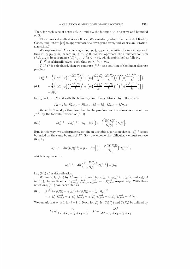
FIG. 7.1. The first sequence of images represents, in the denoising case, from left to right: the degraded image, the synthetic image before degradation, and the reconstructed images with φ1 and φ2. The second represents, from left to right: the degraded image an d the reconstructed image; from top to bottom, the deblurring case and both denoising and deblurring, with φ1.

Now, to compute f n+1 as the solution of this linear system, we can use, for

example, the relaxation method [see 7].Remark . In these algorithms, there are two parameters, λ and h. We denote

λ

= λh2. For the moment, there are not any rigorous choices for the values of λ

andh. But, in practice, we have observed that (as is natural), by decreasing h, the edgesare better preserved and also, by decreasing λ

, we diffuse the image.

7. Experimental results. Finally, we present some numerical results on twoimages of varying difficulty. To generate the images, we have used the softwareMegawave from CEREMADE, at the University of Paris-Dauphine. The first im-age is a synthetic picture (71×71 pixels) with geometric features (like circles, lines,squares). The second is a real image (256×256 pixels) representing a photograph of an office. We have introduced in these pictures the types of degradation consideredhere: standard noise, Gaussian blur (the atmospheric turbulence blur type) or both,and we have made the choice of the parameters λ and h in order to increase thesignal to noise ratio. We remark that in the denoising case, we obtain the results veryfast (in just three iterations), and we obtain good results in the deblurring case. If the degradation involves both noise and blur, the choice of the parameters is moredifficult, because we must take a small λ

in order to obtain a denoising image but,in the same time, λ

must be large to deblur the image. The results for the syntheticimage are all represented in Figure 7.1.




y = 0.00000070.000000

x = 0

255.000000

y = 0.00000070.000000

x = 0

255.000000

y = 0.00000070.000000

x = 0

255.000000

(a)

y = 0.00000070.000000

x = 0

255.000000

y = 0.00000070.000000

x = 0

255.000000

y = 0.00000070.000000

x = 0

255.000000

(b)

y = 0.00000070.000000

x = 0

255.000000

y = 0.00000070.000000

x = 0

255.000000

y = 0.00000070.000000

x = 0

255.000000

(c)

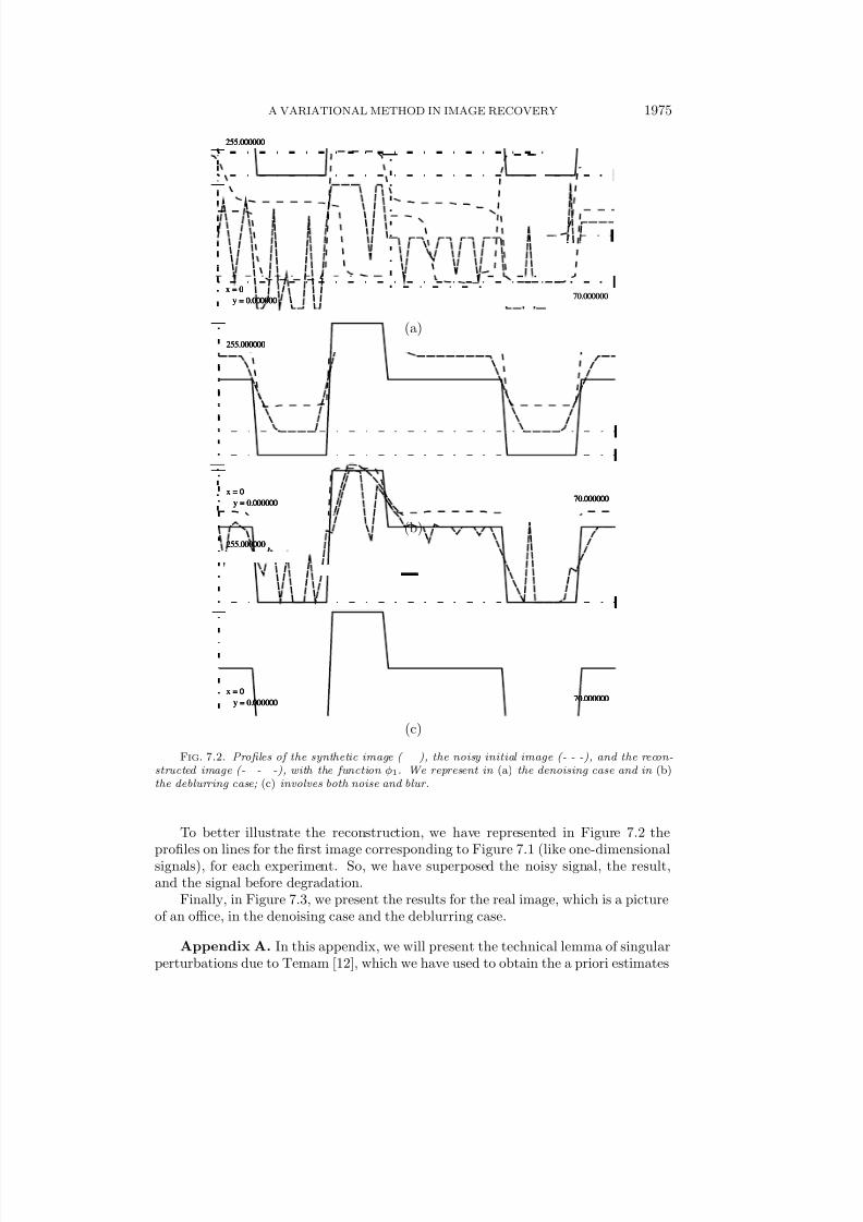
FIG. 7.2. Profiles of the synthetic image ( ), the noisy initial image (- - -), and the recon-structed image (- - -), with the function φ1. We represent in (a) the denoising case and in (b)the deblurring case; (c) involves both noise and blur.

To better illustrate the reconstruction, we have represented in Figure 7.2 the

profiles on lines for the first image corresponding to Figure 7.1 (like one-dimensionalsignals), for each experiment. So, we have superposed the noisy signal, the result,and the signal before degradation.

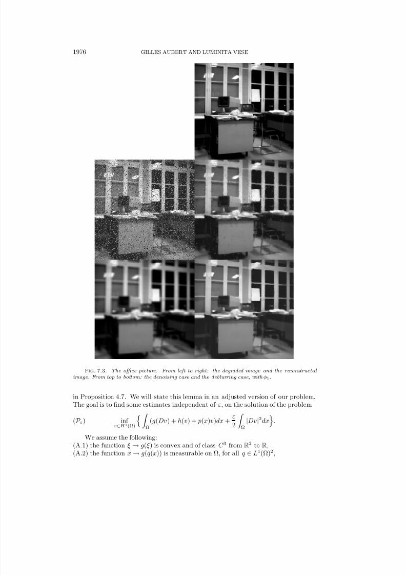
Finally, in Figure 7.3, we present the results for the real image, which is a pictureof an office, in the denoising case and the deblurring case.

Appendix A. In this appendix, we will present the technical lemma of singularperturbations due to Temam [12], which we have used to obtain the a priori estimates




FIG. 7.3. The office picture. From left to right: the degraded image and the reconstructed image. From top to bottom: the denoising case and the deblurring case, with φ1.

in Proposition 4.7. We will state this lemma in an adjusted version of our problem.

The goal is to find some estimates independent of ε, on the solution of the problem

(P ε) inf v∈H 1(Ω)

Ω

(g(Dv) + h(v) + p(x)v)dx +ε

2

Ω

|Dv|2dx

.

We assume the following:(A.1) the function ξ → g(ξ ) is convex and of class C 3 from R

2 to R,(A.2) the function x → g(q (x)) is measurable on Ω, for all q ∈ L1(Ω)2,




(A.3) there exist constants µi ≥ 0, i = 0, 8, such that, for all ξ ∈ R2,

(A.31) g(ξ ) ≥ µ0|ξ | − µ1, µ0 > 0,

(A.32)

∂g

∂ξ i (ξ ) ≤ µ2, i = 1, 2,

(A.33)

2i=1

∂g

∂ξ i(ξ )ξ i ≥ µ3(1 + |ξ |2)

1

2 − µ4, µ3 > 0,

(A.34)µ6|η |2

(1 + |ξ |2)1

2

≤i,j

∂ 2g

∂ξ i∂ξ j(ξ )ηiηj ≤ µ7|η |2

(1 + |ξ |2)1

2

∀η ∈ R2, µ6, µ7 > 0,

where |η |2 = |η|2 − (η·ξ)2

1+|ξ|2,

(A.35) pW 1,∞(Ω) ≤ µ8,

2

i=1

∂g

∂ξ i

(ξ )ξ i

≥0

∀ξ

∈R2,(A.4)

the function t → h(t) is convex and h

(0) = 0.(A.5)

LEMMA A.1 (Temam [12]). The problem P ε has a unique regular solution uεbounded independently of ε in L∞(Ω)

W 1,1(Ω). Moreover, for any relatively compact

open set O in Ω, there is a constant K (O, Ω) such that

uεW 1,∞(O) ≤ K,

uεH 2(O) ≤ K.

We can apply this lemma to our problem by taking, in Proposition 4.7,

g(ξ ) = φ(|ξ |) and h(t) = t2.

We will not give the proof of this lemma. We refer the reader to the paper andthe very technical proofs of Temam. We simply recall that the idea (due to Bernstein)is to obtain some fine estimates on the function vε = |Duε|2. To do this, we use theEuler equation associated with (P ε), which can be written as

(Eε) −ε uε −2i=1

∂

∂xi

∂g

∂ξ i(Duε)

= −h

(uε) − p(x).

We derive (Eε) with respect to xl; then we multiply the result by ∂uε∂xl

and we addover l, with 1 ≤ l ≤ 2, to get

(Bε)ε

2

2

j=1

∂

∂xj

∂vε

∂xj+ ε

2

j=1

2

l=1

∂ 2uε

∂xl∂xj2

−

1

2

2

i=1

∂

∂xi

2

j=1

∂ 2g

∂ξ i∂ξ j

∂vε

∂xj

+

2l=1

2i=1

2j=1

∂ 2g

∂ξ i∂ξ j

∂ 2uε∂xl∂xj

∂ 2uε∂xl∂xi

= −h

(uε)vε −2l=1

∂p

∂xl

∂uε

∂xl

.

The equation (Bε) allows us to obtain the estimates on vε by using the test func-tions judiciously selected and the complicated but classical techniques of Ladyzenskayaand Uralceva [17]. To conclude, we remark that the assumption (A.5) was not given




by Temam. The Temam assumptions on the integrand dependence in v do not allowus to directly apply its result.

To overcome this difficulty, we have assumed (A.5), and then the term h

(uε)vεin (Bε) is not negative, which allows us to obtain all the a priori estimates proved by

Temam.

Appendix B. In the previous sections we studied the problem of image recon-struction when the operator R = I (corresponding to a denoising problem). If R = I (generally a convolution operator), the existence and uniqueness results of section 4remain true if R satisfies the following hypotheses:

(1) R is a continuous and linear operator on L2(Ω);(2) R does not annihilate constant functions.For the results of section 4, we must suppose in addition that(3) R is injective.We do not reproduce the proofs; instead we leave it to the readers to convince

themselves.

Acknowledgments. We would like to thank the referees for useful remarks onthe first version of the manuscript.

REFERENCES

[1] L. ALVAREZ AND L. MAZORRA, Signal and image restoration using shock filters and anisotropic diffusion , SIAM J. Numer. Anal., 31(1992), pp. 590–605.

[2] F. CATTE, P. L. LIONS, J. M. MOREL, AND T. COLL, Image selective smoothing and edge detection by nonlinear diffusion , SIAM J. Numer. Anal., 29(1992), pp. 182–193.

[3] A. CHAMBOLLE AND P. L. LIONS, Image Recovery via Total Variation Minimization and Related Problems, Numer. Math., Vol. 76, 2(1997), pp. 167–188.

[4] P. CHARBONNIER, Reconstruction d’image: Regularisation avec prise en compte des disconti-nuitis, Ph.D. thesis, University of Nice-Sophia Antipolis, 1994.

[5] P. CHARBONNIER, G. AUBERT, L. BLANC-FERAUD, AND M. BARLAUD, Two deterministic half-quadratic regularization algorithms for computed imaging , First IEEE Internat. Conf.

on Image Processing, Vol. II, Austin, TX, IEEE, Piscataway, NJ, 1994, pp. 168–172.[6] P. CHARBONNIER, L. BLANC-FERAUD, G. AUBERT, AND M. BARLAUD, Deterministic edge-

preserving regularization in computed imaging , IEEE Trans. Image Processing, 6(1997),pp. 298–311.

[7] P. G. CIARLET, Introduction a l’analyse numerique matricielle et a l’optimisation , Masson,Paris, 1990.

[8] M. CRANDALL, H. ISHII, AND P. L. LIONS, User’s guide to viscosity solutions of second order partial differential equations, Bull. Amer. Math. Soc., 27(1992), pp. 1–67.

[9] J. P. CROUZEIX, A relationship between the second derivatives of a convex function and of itsconjugate , Math. Programming, 13(1977), pp. 364–365.

[10] B. DACOROGNA, Direct Method in the Calculus of Variations, Springer-Verlag, Berlin, 1989.[11] F. DEMENGEL AND R. TEMAM, Convex functions of a measure and applications, Indiana Univ.

Math. J., 33(1984), pp. 673–709.[12] I. EKELAND AND R. TEMAM, Analyse convexe et problhmes variationnels, Dunod-Gauthier-

Villars, Paris, 1974.[13] S. GEMAN AND D. GEMAN, Stochastic relaxation, Gibbs distribution and the bayesian restora-

tion of images, IEEE Trans. Pattern Anal. Machine Intell., 6(1984), pp. 721–741.[14] D. GEMAN AND C. YANG, Nonlinear Image Recovery with Half-Quadratic Regularization and

FFt’s, preprint, 1993.[15] D. GEMAN AND G. REYNOLDS, Constrained restoration and the recovery of discontinuities,

IEEE Trans. Pattern Anal. Machine Intell., 14(1992), pp. 367–383.[16] D. GILBARG AND N. S. TRUDINGER, Elliptic Partial Differential Equations of Second Order ,

Springer-Verlag, Berlin, 1983.[17] O. A. LADYZENSKAYA AND N. N. URALCEVA, Equations aux derivees partiel les de type el lip-

tique , Dunod, Paris, 1968.




[18] L. LAZAROAIA-VESE, Variational Problems and P.D.E.’s in Image Analysis and Curve Evo-lution , Ph.D. thesis, University of Nice-Sophia Antipolis, 1996.

[19] J. L. LIONS AND E. MAGENES, Problemes aux limites non homogenes, Dunod, Paris, 1968.[20] P. PERONA AND J. MALIK, Scale-space and edge detection using anisotropic diffusion , IEEE

Trans. Pattern Anal. Machine Intell., 12(1990), pp. 629–639.

[21] R. T. ROCKAFELLAR, Convex Analysis, Princeton University Press, Princeton, NJ, 1970.[22] S. OSHER AND L. RUDIN, Total variation based image restoration with free local constraints,

Proc. IEEE Internat. Conf. on Image Processing, Vol. I, Austin, TX, IEEE, Piscataway,NJ, 1994, pp. 31–35.

[23] L. RUDIN, S. OSHER, AND E. FATEMI, Nonlinear total variation based noise removal algo-rithms, Phys. D, 60(1992), pp. 259–268.

[24] G. STAMPPACHIA, Equations elliptiques du second ordre a coefficients discontinus, Presses del’Universite de Montreal, Canada, 1966.

[25] R. TAHRAOUI, Regularite de la solution d’un probleme variationnel , Ann. Inst. H. PoincareAnalyse Non Lineaire, 9(1992), pp. 51–99.

[26] R. TEMAM, Solutions generalisees de certaines equations du type hypersurfaces minima , Arch.Rational Mech. Anal., 44(1971), pp. 121–156.

[27] A. N. TIKHONOV AND V. Y. ARSENIN, Solutions of Ill-Posed Problems, Wiley, New York,1977.

[28] A. VISINTIN, Strong convergence results related to strict convexity , Comm. Partial DifferentialEquations, 9(1984), pp. 439–466.

[29] C. R. VOGEL AND M. E. OMAN, Iterative Methods for Total Variation Denoising , preprint,1994, submitted to IEEE Trans. on Image Processing.

Documents

Calculus if variations