1225 Observatory Drive, Madison, Wisconsin 53706 608-262-3581 / www.lafollette.wisc.edu

The La Follette School takes no stand on policy issues; opinions expressed in this paper reflect the views of individual researchers and authors.

Robert M.

La Follette School of Public Affairs at the University of Wisconsin-Madison

Working Paper Series La Follette School Working Paper No. 2015-005 http://www.lafollette.wisc.edu/research-public-service/publications

Monetary Policy Spillovers and the Trilemma in the New Normal: Periphery Country Sensitivity to Core Country Conditions

Joshua Aizenman University of Southern California and National Bureau of Economic Research

Menzie D. Chinn Professor, La Follette School of Public Affairs and Department of Economics at the University of Wisconsin-Madison, and National Bureau of Economic Research mchinn@lafollette.wisc.edu

Hiro Ito Portland State University April 2015

 

April 21, 2015

Monetary Policy Spillovers and the Trilemma in the New Normal: Periphery Country Sensitivity to Core Country Conditions

Joshua Aizenman*, Menzie D. Chinn†, Hiro Ito‡

USC and NBER; UW-Madison and NBER; Portland State University

Abstract

We investigate why and how the financial conditions of developing and emerging market countries (peripheral countries) can be affected by the movements in the center economies - the U.S., Japan, the Eurozone, and China. We apply a two-step approach. First, we estimate the sensitivity of countries’ financial variables to the center economies, controlling for global and domestic factors. Next, we examine the association of the estimated sensitivity coefficients with the macroeconomic conditions, policies, real and financial linkages with the center economies, and the level of institutional development. In the last two decades, for most financial variables, the strength of the links with the center economies have been the dominant factor. While certain macroeconomic and institutional variables are important, the arrangement of open macro policies such as the exchange rate regime and financial openness are also found to have direct influence on the sensitivity to the center economies. We also find, among other results, that an economy that pursues greater exchange rate stability and financial openness faces a stronger link with the center economies. Nonetheless, exchange rate regimes have mostly indirect effects on the strength of financial linkages. We conclude the trilemma remains relevant.

                                                            * Aizenman: Dockson Chair in Economics and International Relations, University of Southern California,

University Park, Los Angeles, CA 90089-0043. Phone: +1-213-740-4066. Email: aizenman@usc.edu. † Chinn: Robert M. La Follette School of Public Affairs; and Department of Economics, University of

Wisconsin, 1180 Observatory Drive, Madison, WI 53706. Email: mchinn@lafollette.wisc.edu . ‡ Ito (corresponding author): Department of Economics, Portland State University, 1721 SW Broadway,

Portland, OR 97201. Tel/Fax: +1-503-725-3930/3945. Email: ito@pdx.edu .

Acknowledgements: The financial support of faculty research funds of University of Southern California, the University of Wisconsin, Madison, and Portland State University is gratefully acknowledged. We also thank Ting Ting Lu for her excellent research assistance, Clas Wihlborg and Arnaud Mehl for helpful comments, and Jing Cynthia Wu, Fan Dora Xia, Jens Christensen, and Glenn D. Rudebusch for sharing the shadow interest rate data. An earlier version of this paper circulated as “Analysis on the Determinants of Sensitivity to the Center Economies.” All remaining errors are ours.

 

1  

1. Introduction

The integrated nature of the financial system was amply demonstrated by the turmoil in

emerging market currency and bond markets in the wake of Fed Chairman Bernanke’s

statements regarding the normalization of U.S. monetary policy, commonly termed the “taper

tantrum”. Following close on the heels of complaints about unconventional monetary policy

implementation in the preceding years, it is clear that – at a minimum – policymakers in

emerging market economies perceive an increasing vulnerability to the whims of the global

financial system.

The idea that the monetary policies of financial center countries have large spillover

effects on the smaller economies is not new. During the mid-1990’s, when advanced economy

central bankers raised policy rates, after several years of negative real interest rates, similar

complaints were lodged, and some may partly trace the financial crises in Latin America and

subsequently in East Asia to the cycle in core country policy interest rates.

One key difference is that in the earlier episode’s aftermath, the semi-fixed exchange rate

regimes were tagged as a contributing factor. In contrast, countries adhering to a variety of

exchange rate regimes all experienced challenges in insulating their economies in the most recent

episode. This has led to a grand debate about the continued relevance of the “impossible trinity”

or “monetary trilemma”.

Since Mundell (1963) outlined the hypothesis of the monetary trilemma, fundamental

policy management in the open economy has been viewed as policy trade-offs among the choices

of monetary autonomy, exchange rate stability, and financial openness.4 The hypothesis and its

extensions in recent years suggest a continuous trade off between the three trilemma dimensions,

with the possibility that a fourth policy goal, financial stability, may augment it and turn it into a

quadrilemma, where international reserves may play a role as buffers.

In contrast, in the aftermath of the global financial crisis (GFC), Rey (2013) concluded

that the economic center’s (CE) monetary policy influences other countries’ national monetary

policy mostly through capital-flows, credit growth, and bank leverages, making the types of

exchange rate regime of the non-CEs irrelevant. In other words, the countries in the periphery

(PH) are all sensitive to a “global financial cycle” irrespective of exchange rate regimes. In this

                                                            4 See Aizenman, et al. (2010, 2011, 2013), Obstfeld (2014), Obstfeld, et al. (2005), and Shambaugh (2004) for further discussion and references dealing with the trilemma.

 

2  

view, the “trilemma” reduces to an “irreconcilable duo” of monetary independence and capital

mobility. Consequently, restricting capital-mobility maybe the only way for non-EC countries to

retain monetary autonomy. The recent experience of Brazil, India, Indonesia, South Africa, and

Turkey – the “Fragile Five” – during the so called taper tantrum may make many observers the

“irreconcilable duo” view convincing.

In this paper we investigate whether Rey’s prematurely predicted the end of the trilemma.

Inferences based data drawn from times of heightened volatility emanating from the center might

be modified once we examine how the propagation of large shocks from the EC can be affected

by economic structures and measures of the trilemma variables. In a world of more than hundred

countries, one ignores heterogeneity at one’s own risk. For instance, the trade-offs facing the

OECD countries may differ from those facing manufacturing based or commodity based

emerging markets economies and developing countries.5 Furthermore, large shocks arising from

the EC during the global financial crisis and the Euro debt crisis may have altered the

transmission dynamics, especially in comparison to the preceding decade of illusory tranquility.

We first review key global developments in the past decades and preview our

methodology and the main empirical results. We begin with Figure 1 which illustrates the 36-

month rolling correlations of domestic money market rates with the U.S. money market rate for

developed countries (IDC), developing countries (LDC), and emerging market economies

(EMG), and China, from 1990 to 2013. For developed economies, the correlation between

domestic and the U.S. policy interest rates is high and hovers at relatively high levels in the last

decade. In contrast, developing countries tend to retain high monetary independence from the

U.S., while emerging market monetary policy independence occupies a middle ground. All the

correlations fluctuate, but experience two pronounced dips in recent years, one in 2005 and the

other at the time of the global financial crisis. These two dips correspond to rapid changes in the

U.S. Federal funds rate.6

Figure 2 depicts correlations of long-term interest rates. Again, the long-term interest

rates of industrialized countries register high correlations with that of the U.S., particularly in the

                                                            5 For example, maintaining exchange rate stability could be more important for developing countries whose growth strategy is reliant on the exports of a narrower variety of manufactured goods or commodities than advanced economies with more diversified economic structures. 6 The Federal Reserve started raising the federal fund rate target from 1.00% in June 2004 to 5.25% in June 2006. It started lowering the target from 5.25% in September 2007 all the way essentially to the 0.00-0.25 by December 2008.

 

3  

first half of the sample period, though the correlation has been on a rising trend again in recent

years. Developing countries experience relatively high correlations in the early 2000s but since

the late 2000s, the correlations appear to be trendless for these countries. Long-term interest rates

across countries, including both developed and developing countries, were highly correlated

during the Great Moderation period.

Figure 3 is an interesting picture. It illustrates the comparable correlations of stock

market price indexes (expressed in local currency) with the U.S. index. Since the mid-2000s, all

the country groups have maintained high levels of correlations of stock market price indexes

with the U.S. stock market, with some tail-off since the global financial crisis.

What do these figures tell us? Broadly speaking, the extent of correlations is the highest

for stock market price movements, followed by the long-term and short-term interest rates.

Given short-term interest rates bear lowest levels of risks, we may conjecture that the prices of

assets with higher risk tend to be more highly correlated with that of the United States. Of course,

these graphical depictions do not provide conclusive evidence, particularly since we have not

controlled for any number of important factors, e.g., the policy regimes, macroeconomic

conditions, the extent of trade linkage, the level of institutional development and size of financial

markets, and global market conditions.

Many studies such as Ahmed and Zlate (2013), Forbes and Warnock (2010), Fratzscher

(2011), and Ghosh, et al. (2012) have documented the importance of global factors such as

advanced economy interest rates and global risk appetite in affecting capital flows to small open

economies. Nonetheless, these studies have also highlighted that domestic, country-specific

factors also retain importance. In particular, the institutional and macroeconomic policy

frameworks of the emerging market economies also determine the variations in flows.

Given this context, we focus on the questions of why movements in the major advanced

economies often have large effects on other financial markets, how these cross-market linkages

have changed over time, and what kind of factors contribute to explaining the sensitivity to the

movements in the major economies. More specifically, we will conduct an empirical analysis on

what determines the sensitivity of economies to factors pertaining to the core economies in the

world, namely, the U.S., the Euro area, Japan, and China.

For the last two decades, the Chinese economy has been growing at impressive rates and

quickly moving upward on the development ladder. However, its financial markets may not be

 

4  

developed or sophisticated to the extent of becoming the center of global financial cycles.

Despite data limitations as well as China’s relatively short tenure as one of the G3 countries, we

will also examine whether our results are sensitive to the inclusion of China as one of the center

economies.

For our empirical exploration, we employ an estimation process similar to that employed

by Forbes and Chinn (2004), which is composed of two steps of estimations. First, we investigate

the degree to which the sensitivity of several important financial variables to global, cross-

country, and domestic factors. Second, treating the estimated sensitivity as a dependent variable,

we will examine their determinants among a number of country-specific variables. In so doing,

we will disentangle roles of countries’ macroeconomic conditions or policies, real or financial

linkage with the center economy, or the level of institutional development of the countries.

In Section 2, we will detail the framework of the two stage estimation exercise. We will

report and discuss the estimation results in section 3. In Section 4, we will make concluding

remarks.

To anticipate the results, we find that for most of the financial variables we examine, the

strength of the links with the center economies have been the dominant factor over the last two

decades. The influence of global financial factors, for which we use VIX and Ted spread, has

been increasing since around the time of the global financial crisis. The results we obtain suggest

that, across different financial linkages, higher levels of direct trade linkage, financial

development, and gross national debt all tend to lead to stronger financial linkages between the

sample countries and the three center economies. Open macro policy arrangements such as the

exchange rate regime and financial openness also affect the extent of financial linkage both

directly and indirectly, i.e., interactively with other macroeconomic or institutional variables.

Specifically, we do find that the types of exchange rate regimes do affect the extent of sensitivity

to changes in financial conditions or policies in the center economies. Hence, the open macro

policy choice is “still” dictated by the hypothesis of the trilemma, so that we yet need to reduce

the trilemma to a dilemma between monetary autonomy and financial integration.

2. The Empirical Methodology

2.1 The First-Step: Estimating Sensitivity Coefficients

 

5  

The main objective of this first step estimation is to estimate the correlation of a specific

financial variable between country i and each of the center economies while controlling for

global and domestic factors. The estimated coefficient of our focus is CFi . A significantly

positive CFi indicates a closer linkage between country i and economic center country C, as

shown in (1):

ititFit

C

c

Cit

CFit

G

g

Git

GFitFit

Fit YXZR

11

. (1)

Where the GiZ is a vector of global factors, the C

iX is a vector of cross-country factors, and Yit is a

control variable for domestic factors. C represents the center economies: the U.S., the Euro area,

Japan, and China. Cii is the estimate of our focus and represents the extent of sensitivity of a

financial variable ( FitR ) to cross-country factors, or more specifically, linkages to the four major

economies.

As for the financial variable as the dependent variable, we are interested in 1) the short-

term policy interest rate; 2) stock market price changes; 3) the sovereign bond spread; and 4) the

rate of change in the real effective exchange rate (REER).

We use money market rates to represent policy short-term interest rate. In recent years,

all of the advanced major economies, the U.S., the Euro area, and Japan have implemented

extremely loose monetary policy in the aftermath of the global financial crisis (GFC). Given that

both the U.S. and Japan have lowered their policy interest rates down to zero or near zero, using

official policy interest rates may not capture the actual state of monetary policy. In recent years,

many researchers have estimated “shadow interest rates” to represent the actual state of liquidity

availability by allowing the estimated shadow rates to drop below the zero bound. We use these

shadow rates for the three advanced economies to estimate more realistic correlations between

the policy interest rates of the center economies and sample countries. For the U.S. and the Euro

area, we use the shadow interest rates estimated by Wu and Xia (2014). For Japan, we use the

shadow rates estimated by Christensen and Rudebusch (2014).7

                                                            7 For the U.S. policy interest rates, we use the shadow rates for the entire sample period – the shadow rates deviate from the actual Federal Fund Rate more substantially only after the policy rates hit the zero bound. For the Euro area,

 

6  

For stock market prices, we use stock market price indices reported in the IMF’s

International Financial Statistics (IFS). The (sovereign) term spread is the difference between

the long-term interest rate (usually 10 year government bond) and the policy short-term interest

rate – i.e., the slope of the yield curve. We use the REER indices from the IFS.

For a vector of global factors ( GiZ ), we have two subsets of global factors. The first

subset of global factors include “real” variables -- global interest rates (for which we will use the

first principal component of U.S. Federal Reserve, ECB, and Bank of Japan’s policy interest

rates); oil prices; and commodity prices. To avoid multicollinearity or redundancy, we also

calculate the first principal component of oil and commodity prices and use the resultant variable

as a control variable for input or commodity prices.8

The second subset is “financial.” In this group, we include the VIX index from the

Chicago Board Options Exchange (CBOE), as a proxy for the extent of investors’ risk aversion,9

and the “Ted spread,” which is the difference between the 3-month Eurodollar Deposit Rate in

London (LIBOR) and the 3-month U.S. Treasury Bill yield. This latter measure gauges the

general level of stress in the money market for financial institutions. The same set of global

factors, except for the principal components of the global interest rates, is used for all the

estimations regardless of the dependent variable.

The vector of cross-country linkage factors (XC) corresponds to the dependent variable.

For example, if the short-term interest rate for country i is the dependent variable, CiX includes

the short-term interest rates of the four center economies.10 We implement the estimation for

each of the sample countries for the four different dependent variables and for a sample period of

either three or five-year panels (p). To control for domestic economic conditions, we include the

year-on-year growth rate of industrial production index.

All the data used for this estimation exercise are monthly frequency. The same set of

explanatory variables (except for the world interest rate) is regressed against the four financial

                                                                                                                                                                                                we use the estimated shadow rates only after the introduction of the Euro. For Japan, we use the shadow rates after 1996, before which we assume the shadow rates do not deviate substantially from the actual policy rates. 8 When we estimate for the policy interest rate correlation, we do not include the first component of U.S. FRB, ECB, and Bank of Japan’s interest rates as part of the global factor vector because it would overlap with XC. 9 The VIX index series starts in 1990, but we use the VXO index, an older version of the VIX index, to extrapolate the VIX index to 1986. The correlation between the two indices is about 99%. A higher VIX index indicates a higher level of risk appetite. 10 For the Euro Area’s variables, before the introduction of the euro in 1999, the GDP-weighted average of the variable of concern for the original 12 Euro countries is calculated and included in the estimation.

 

7  

variables: policy interest rate, the rate of change in stock market price indices and the rate of

change in the REER index, and sovereignty bond spread.

Because we deal with a relatively long sample period, coefficient instability is a concern.

Hence, we estimate period specific regressions in each of the three and five year panels, starting

in 1986 in the case of three-year panels.11 That means that CFit is time-varying across the panels.

For the rest of the paper, we focus on the results from the estimations on the three-year panels

since the results from five-year panels are qualitatively similar.

We also estimate two specifications. One specification excludes China as one of the

“center economies.” In this model setup, we are testing the sensitivity of our sample economies

to the traditionally-defined major economies of the U.S., the Euro area, and Japan. Excluding

China mitigates data limitations as well, especially for the second-step of the estimation

procedure. The other model does include China as one of the center economies.12

We estimate equation (1) to a group of about 100 countries including both advanced

economies (IDC) and less developed countries (LDC), though the number of countries included

in the four models differs depending on data availability. In our sample, the U.S. and Japan are

not included in any of estimates. Moreover, China is excluded for the specificaiotn in which

China is included as one of the major economies. As for the Euro member countries, they are

removed from the sample after the introduction of the euro in January 1999 or when they become

member countries, whichever comes first. We also have a subsample of emerging market

countries (EMG) within the LDC subsample.13

2.2 The Second Step: Explaining the Sensitivity Coefficients

Once we estimate CFit for each of the four dependent variables for all the samples, we

regress CFit on a number of country-specific variables.

FitFitFitFitFitFitCFit uCRISISINSTLINKMCOMP 543210ˆ (2)

                                                            11 In the case of five year intervals, the first panel starts in 1985 and is composed of three years: 1985-1987, and after that, five-year periods are constituted: 1988-1992, 1993-1997, 1998-2002, 2003-2007, and 2008-2012. 12 Including China changes the sample periods when the dependent variable is stock market price index changes, as a consequence of data limitations. 13 The emerging market countries (EMG) are defined as the countries classified as either emerging or frontier during the period of 1980-1997 by the International Financial Corporation plus Hong Kong and Singapore.

 

8  

There are four groups of explanatory variables. The first group of explanatory variables is

a set of open macroeconomic policy choices ( iOMP ), for which we include the indexes for

exchange rate stability (ERS) and financial openness (KAOPEN) from the trilemma indexes by

Aizenman, et al. (2013).14 A country that has a fixed exchange rate arrangement with a major

country, or the base country, is more subject to financial shocks occurring to the base country if

it has more open financial markets. Saxena (2008) found the extent of pass-through from foreign

interest rates to domestic interest rates is higher under floating exchange rate regimes than

pegging regimes, however.15 Christiansen and Pigott (1997) also suggest that even under floating

exchange rate regimes, foreign factors play an important role in affecting long-term interest rates.

Hence, it is an empirical question how and to what extent both financial openness and exchange

rate stability matter for transmitting financial shocks. As another variable potentially closely

related to the trilemma framework, we suspect the level of international reserves (IR) holding

may affect the extent of cross-country financial linkages and include a variable for IR holding

(excluding gold) as a share of GDP. Aizenman, et al. (2010, 2011) show the macroeconomic

impact of trilemma policy configurations can depend upon the level of IR holding.

The group iMC includes macroeconomic conditions such as inflation volatility, current

account balance, and public finance conditions. As the measure of public finance conditions, we

include either gross national debt, or general budget balance, both expressed as shares of GDP.

These variables are included as deviations from the major economies. We use the data from the

IMF’s International Financial Statistics and World Economic Outlook Database.

In addition to these groups of variables, we will include variables that reflect the extent of

linkages with the center countries (LINK). One linkage variable is meant to capture real, trade

linkage, which we will measure as: ipC

ipip GDPIMPLINKTR _ where CiIMP is total imports into

                                                            14 As Mundell (1963) argued and Aizenman, et al. (2013) and Ito and Kawai (2012) have empirically shown it holds, a country may simultaneously choose any two, but not all, of the three goals of monetary policy independence, exchange rate stability, and financial market openness to the full extent. Given this linearity, we only include the two trilemma indexes out of the three. On the trilemma, also see Obstfeld (2014), Obstfeld, Shambaugh, and Taylor (2005) for further discussion and references dealing with the trilemma. 15 To explain the counterintuitive results, Saxena argues that the classification of exchange rate regimes may allow some of the countries that conduct active but incomplete foreign exchange interventions to be classified as “floating” regimes so that the results for the floating regimes may include those of de facto pegging regimes. Also, she argues countries with floating exchange rates tend to have more developed financial markets which tend to follow the trend of the center country’s financial markets.

 

9  

center economy C from country i, that is normalized by country i’s GDP. Another linkage

variable is financial linkage, FIN_LINKip. For one, we will measure it with the ratio of the total

stock of bank lending from country C in country i as a share of country i’s GDP ( CiBL ) for which

we use the BIS consolidated banking statistics data. As another variable of financial linkage, we

also use the ratio of the total stock of foreign direct investment from country C in country i as a

share of country i’s GDP ( CiFDINV ).16

Another variable that also reflects the linkage with the major economies is the variable

for the extent of trade competition (Trade_Comp). Trade_Comp measures the importance to

country i of export competition in the third markets between country i and major country c.

Shocks to country c, and especially shocks to country c that affects country c’s exchange rate,

could affect the relative price of country c’s exports and therefore affect country i through trade

competition in third markets. See Appendix for the variable construction. A higher value of this

measure indicates country i and major economic c exports products in similar sectors so that

their exported products tend to be competitive to each other.

Theoretical prediction of this variable is not straightforward. For example, if a major

economy lowers its policy interest rate, that would help depreciate the major economy’s currency

and therefore make its exports more competitive. If country i tends to export similar products in

terms of the aggregated industrial sectors, which may also lead to a fall in the policy interest rate

of country i, which makes a positive estimated coefficient on this variable. However, if a fall in

the policy rate in this example foresees some underperforming productivity growth in the future,

that may make competitors’ exports appear more attractive. A rise in the demand for competitors’

exports may lead a rise in the policy interest rate, making the expected sign of the estimate for

the correlation of the policy interest rates negative.

The fourth group is composed of the variables characterize the nature of institutional

development (INST), namely, variables for financial development and legal development. As

Caballero-Farhi-Gourinchas (2008) theoretically predict and Chinn and Ito (2007) empirically

show, both Financial and legal development are important factors for the volume and directions

of cross-border capital flows. Alfaro, et al. (2008) argue that institutional development is also an

                                                            16 Among the financial link variables, the variable for bank lending provided by the center economies turned out to be persistently insignificant across different estimation models. Therefore, we decided to drop the variable from the models.

 

10  

important factor. If these factors affect cross-border capital flows, they should also affect the

extent of sensitivity to financial shocks occurring to the center economies.

There is no agreement about what would be the best way to measure the extent of

financial development, because the development of financial markets can be gauged in terms of

size, depth, activeness, unit or transaction costs, and profitability to name a few. Here, to

measure the level of financial development, we calculate a composite index, or the first principal

component, of financial development (FD) using the data on private credit creation, stock market

capitalization, stock market total value, and private bond market capitalization all as shares of

GDP. Additionally, we also include a measure of legal development, for which we use LEGAL

which is the first principal component of law and order (LAO), bureaucratic quality (BQ), and

anti-corruption measures (CORRUPT), all from the ICRG database.17

The precision of CFit could be reduced by economic or financial disruptions. To control

for that, we include a vector of currency and banking crises (CRISIS). We use the crisis dummies

from Aizenman and Ito (2013) to identify the two types of the crises. For currency crisis,

Aizenman and Ito use the exchange market pressure (EMP) index using the exchange rate

against the currency of the base country. The banking crisis dummy is based on the papers by

Laeven and Valencia (2008, 2010, 2012).

For each of the four financial variables we estimated in the first-step regression, we have

(i × C × t) ’s where t refers to either three- or five-year panels and C is four when we include

China as a major economy and three if not. The variables in MC and INST are included in the

estimations as differences from the U.S., Japanese, Chinese, and Euro Area’s counterparts. The

variables in vectors OMP, MC, and INST are sampled from the first year of each three (or five)

year panels to minimize the effect of potential endogeneity. Also, to capture global common

shocks, we also include time fixed effects.

As we previously mentioned, our discussions focus on the results from three-year panel

estimations. For each of the three- or five-year panels, we average all the explanatory variables.18

By so doing, we will essentially form non-overlapping three- or five-year panels.

                                                            17 Higher values of these variables indicate better conditions. 18 As for the crisis dummies, if a crisis occurs in any year within the three- or five-year period, we assign the value of one.

 

11  

3. Empirical Results

3.1 First-Step Estimations

The Contributions of Different Factor Vectors

For the first-step estimation, we have four variables to estimate: policy interest rate, stock

market price changes, REER changes, and sovereignty debt spread. We regress each of these

dependent variables on four groups of explanatory variables: real global, financial global, cross-

country link, and domestic factors for three-year, non-overlapping panels in the 1986-2012

period.19

To grasp the general trend of the groups of factors that influence the four financial

variables, we focus on the joint significance of the variables included in the real global, financial

global, cross-country, and domestic groups. Figure 4 illustrates the proportion of countries for

which the joint significance tests are found to be statistically significant (with the p-value less

than 10%) for each of the four financial variables. These figures are based upon the specification

that includes China as a major economy while the figures based on the specification without

China as a center economy yields similar observations. The figure illustrates the proportion for

the groups of advanced economies (IDC) and less developed economies (LDC) after 1992.20

These graphical depictions lead to the following four conclusions. First, the movements

of the financial variables of the center economies not only matter for all of the four financial

variables, but contribute the most among the groups of explanatory variables to jointly

explaining the variation of the variables for both the IDC and LDC groups. Among the LDC

economies, the influence of the major economies appears to be the greatest for the policy interest

rates, though it tends to be high also for term spreads and real effective exchange rates and less

so for stock market price changes.21 While the policy interest rate specification indicates for the

LDC economies that the levels of joint significance remain constantly high throughout the

sample period, the influence of the major economies increased markedly in the last two three-

year periods in the specifications for the other three financial variables. In the model of stock

market price changes, the major economies’ influence appears to be relatively smaller than in the                                                             19 For the model that includes China as a center economy, the sample for the stock market price estimation starts in 1992 due to data availability. 20 The figures for the EMG group are qualitatively similar to those of the LDC group. Hence, we omit discussing them here. 21 When we restrict our sample to emerging market economies (not reported), the contribution of the major economies becomes bigger, which is expected considering that this group of economies have more developed and open financial markets.

 

12  

models for the other three financial variables, reflecting that many of LDC’s stock markets are

less developed, though the proportion of joint significance is now in a moderately rising trend in

the last decade or so.22

Second, as far as policy interest rate is concerned, the proportion of joint significance is

also relatively high for the group of “financial global” variables, especially for the EMG

countries. Unsurprisingly, the last two three-year panels indicate high proportions of joint

significance for both country groups, suggesting global financial factors have been playing an

important role in affecting the policy interest of countries, both developed and developing. This

result is consistent with the Rey’s (2013) thesis of “global financial cycles”. In the panels for

1998-2000 and 2001-2003, the proportions of financial global factors also appear high for both

country groups.23 Given the emerging market crises in the 1998-2000 period, and dot com bust

of the 2001-2003 period, these results suggest that economies are more exposed to global

financial shocks during periods of financial turbulence while also following center monetary

policies.

Third, stock market movements in almost all the developed economies are influenced by

those in the center economies. The fact that many of the countries in this group have highly

sophisticated stock markets explain the high proportion of joint significance.24 Among

developing countries, the proportion of these economies subject to movements in the center

economies is generally lower, though the proportion has been moderately rising over the last

decade.

Fourth, the center economies play a crucially important role for developed economies’

term spreads, although “real global” factors are also influential in the 1990s through the early

2000s, as well as the last three-year post-GFC period. For developing economies, the center

economies’ spreads matter less, though they appear quite influential in the last post-crisis period.

The fact that “real global” factors do not affect the policy interest rates that much while more

influencing the term spreads indicates that “real global” factors must affect longer-term interest

rates.

                                                            22 The rising trend is more discernable for the EMG group. 23 Again, this is more distinct for the EMG group. 24 This subsample includes most of the European Monetary Union members. That also contributes to the high proportion of joint significance.

 

13  

Last, for the changes in the REER, the movements of the center economies are critically

important for both country groups. Interestingly, the highest proportion of developing countries

appear sensitive to the REER movements of the center economies in 2010-2012. These results

are consistent with the reactions expressed by emerging market policy makers to the taper in Fed

quantitative easing.25

Overall, in accord with Rey (2013), these figures suggest that economies, both advanced

and developing, are subject to the financial conditions of the center economies. We investigate

the determinants of the degree of sensitivity to the financial conditions of the center economies

in the next subsection.

Figure 5 provides a closer look at the influences of the center economies. It presents the

proportion of the countries for which the estimated coefficients of the center economies’

variables are found to be significantly positive (with the p-value less than 20%) for each of the

four financial variables ( C >0) and for each of the center economies. We display only the results

for the group of developing countries. The positive estimate indicates that the financial

conditions of the center economies are influential on other non-CE countries. By comparing the

C ’s for different center economies, we can see to which center economy’s financial conditions

the sample countries are more sensitive to.

Policy interest rates in many developing countries appear to be positively correlated with

the Euro area’s policy interest rate in the last three-year period. The high proportion of the

countries with EURO > 0 likely reflects the Euro debt crisis. We also find relatively high

proportions of countries with positive correlations with Euro area stock market price changes,

although unsurprisingly it is the U.S. that affects other countries’ stock market price movements.

The U.S. is also a relatively dominant influence in terms of the real effective exchange

rate movements. The influence of the center economies for term spread is hard to pin down,

except for that, again, the Euro area is a dominant economy in the 2007-09 period.

Contributions of China as a Major Economy

So far, the empirical results illustrated in Figures 4 and 5 are based on the assumption

that China is one of the center economies. However, one can still question whether China’s

                                                            25 Another observation is that the contribution of industrial production growth as the domestic factor is generally low, though it tends to be slightly higher for the policy rate and term spread estimation models.

 

14  

financial influence matches its impact on real activity. Many studies have shown that there is still

much room for China to further develop and open its financial markets.26

Hence, we repeat the previous exercise of testing the joint significance of each vector of

explanatory variables, but excluding China from the group of the center economies (i.e.,

removing the Chinese variable from the cross-country linkage vector). The general

characteristics we observed in Figure 4 remain qualitatively intact, suggesting that the financial

influence of China remains minimal.

To test this assertion more formally, we compare the adjusted R-squared values of the

two specifications for each country and each three-year panel, and for each of the four financial

variables. Figure 6 illustrates the cross-country average differences in the adjusted-R squared

values between the estimation with China as one of the center economies and the one without for

the four financial variables. The averages of the gap are calculated for the groups of developed

countries, developing countries, emerging market countries, and East Asian emerging market

economies as a comparison.27

Overall, the extent of contribution to the adjusted R-squared of including China as one of

the center economies depends on the financial variable examined. Regarding the policy interest

rate and term spread models, including China as a major country increases the adjusted R-

squared, especially in the last three years of the 1990s that correspond to the East Asian crisis.

For East Asian emerging market economies, including the Chinese policy interest rate in the

estimation model increases the adjusted R-squared as much as over 15% on average. Despite the

recent impressive rise as an economic power, however, China’s contribution seems negligible in

the last two three-year panels for both the policy rate and term spread models.

In the REER figure, we see a high increase in the adjusted R-squared in the crisis years of

2007-2009 for emerging market countries, especially those in East Asia (with the additional

contribution of about 18% to the adjusted R-squared). This may reflect the situation where

international trade shrank significantly immediately after the outbreak of the global financial

crisis in 2008. In the tight international trade market, trade competitiveness of the world’s largest

exporter may have had a large influence on other trading partners.

                                                            26 See Huang, et al. (2013) and Hung (2009) among others. 27 The group of East Asian emerging market economies includes: Hong Kong, India, Indonesia, Korea, Malaysia, the Philippines, Singapore, Thailand, and Vietnam.

 

15  

China’s stock markets do not appear influential in most of the sample period, except for

the 2004-2006 period. Given that China’s stock markets only became open recently, the lack of

influence of China’s stock markets is unsurprising.

3.2 Results of the Second-Step Estimation

Now that we have CFit for the four financial variables, we investigate the determinants of

the extent of linkages using the estimation model based on equation (2). We estimate two

specifications with two different dependent variables for each of the four financial variables. The

first type of estimation has the dependent variable of CFi from the first-step estimation that does

not include China as one of the center economies. Hence, for country i in one three-year panel t,

there are three (i.e., USFit , JP

Fit , and EUROFit ), making (i × 3 × t) observations. The second type is

the one for which the first-step estimation is conducted with China included as one center

economy. Hence, for the second-step estimation, country i in one three-year panel t has four CFit

((i × 4 × t) observations in total). In what follows, however, we only report the results from the

specifications without China as a center economy, since we determined the financial influence of

China is minimal. The regressions with China as a center economy yield results qualitatively

similar to those without China.28

Tables 1-1 through 1-3 report the estimation results for the extent of sensitivity of policy

interest rates, stock market price changes, and the REER for the FULL, IDC, LDC, and EMG

samples. We do not report the estimation results for the term spread sensitivity because of the

consistent lack of robust results across different models, especially for the groups of developing

and emerging market countries. The bottom rows of the tables also report the joint significance

tests for each vector of explanatory variables. We will focus our observations on the results for

the subgroups of LDC and EMG.

As for the linkage of policy interest rates, reported in Table 1-1, the variables that

characterize countries’ open macro policies affect the sensitivity to the monetary policies of the

center economies. In contrast with Rey’s argument, we find that the type of exchange rate

regimes does matter; countries with greater exchange rate stability tend to be more sensitive to

changes in the center economies’ monetary policy, though except for model (5), the estimate is

                                                            28 The estimation results with China as a center economy are available from the authors upon request.

 

16  

only marginally significant. Financial openness also contribute to higher degrees of sensitivity to

the center economies’ policy interest rates. Interestingly, holding higher levels of foreign

reserves tend to help peripheral economies to shield the impact of changes in the center

economies’ policy interest rates, i.e., to retain its monetary autonomy. Exchange rate stability,

financial openness, and IR holding are jointly significant for the group of developing or

emerging market countries.

Among the variables for macroeconomic conditions, only current account balance seems

to matter. However, the positive estimate on current account balance appears somewhat puzzling

considering that a country running current account deficit -- not surplus -- is more susceptible to

monetary policy changes of the center economies. The result indicates that a net capital exporter

rather than importer is more sensitive to the monetary policies of the center economies.

Among the factors of external links, financial linkage through foreign direct investment is

the most important variable in determining how shocks to the center economies’ monetary

policies could affect those of other non-center economies for both developing and emerging

market countries. A country that receives more FDI from the center economies tends to be more

sensitive to changes in the monetary policies of the center economies.29

Financial development also matters significantly for the IDC and LDC samples.

Countries with more developed financial markets tend to be more sensitive to the changes in the

monetary policies of the center economies. That suggests that countries with deep financial

markets can be good investment destinations for foreign investors, so that their arbitrage actions

may lead those countries to follow the monetary conditions of the center economies more closely.

Table 1-2 shows that the estimation results for stock market price changes are less robust

and share few characteristics with the model for the policy interest rates. A developing or

emerging market country with larger government debt tends to be more vulnerable to stock

market movements of the center economies, while financial development, if any, seems to help

its market shun shocks arising in the center economies’ markets unlike in the case of policy

interest rates.

The degree of exchange rate stability does matter for stock market price changes, but in a

manner that is a sharp contrast to the policy interest rate model. A country with greater exchange

                                                            29 We dropped cross-bank lending and FDI stock since both variables are found to be persistently insignificant contributors to the extent of sensitivity.

 

17  

rate stability tends to experience a smaller degree of co-movement of stock market prices with

the center economies. This result is somewhat counterintuitive considering that greater exchange

rate stability may leave an economy more susceptible to external financial shocks. However, if a

shock occurs in the center economies, international investors may try to reorganize their

portfolios in the markets where the exchange rate is flexible because the exchange rate risk is

greater than in a fixed exchange rate regime. Financial openness appears to be a negative

contributor, though significantly only in model (5).

Among the external link variables, the degree of trade competition positively affects the

stock market price change link between peripheral and center economies among the group of

developing countries. If a developing country exports products in similar sectors to the center

economies, that country tends to be more vulnerable to changes in stock market prices in the

center economies, possibly reflecting that similar industrial structures should pass around shocks

to stock markets. However, receiving more FDI from the center economies could shun the effects

of the shocks occurring in the center economies’ stock markets.

Generally, the models for REER present results with best goodness-of-fit as Table 1-3

reports. Given certain degrees of price stickiness, pursuing greater exchange rate stability would

lead both nominal and real effective exchange rate to be more sensitive to that of the center

economies. Our results show the positive impact of greater exchange rate stability on the REER

connectivity for all the subsample country groups. Greater financial openness also contributes to

greater sensitivity for developing countries, though not significantly so for the EMG group.

Interestingly, irrespective of group, a country with a higher level of IR holding tends to be more

sensitive to REER changes of the center economies. One interpretation is that a country could

respond to changes in the center economies’ real currency appreciation through foreign exchange

market interventions, inducing a positive correlation; the interpretation of this coefficient is then

not causal.

Emerging market countries with larger government debt or budget deficits tend to be less

sensitive to the REER of the center economies. These results may reflect the fact that such

countries, which likely face higher inflationary expectations, often face some difficulty in

maintaining real exchange rate stabilities against the currencies of the major economies despite

their general desire to pursue greater (nominal) exchange rate stability (Aizenman, et al. 2013,

Calvo, et al. 2000).

 

18  

Not surprisingly, countries with greater bilateral trade links with the center economies

tend to be more sensitive to the REER movements of the center economies. The negative impact

of trade competitiveness means that peripheral countries with more competitive trade structure to

that of the center economies tend to become alternative investment destination if a shock occurs

to the center economies. For example, if a shock happens in a way that causes real depreciation

of the center economies’ currencies such as predicted output growth, an institutional change that

would increase the level of labor rigidities, and a decrease in the appetite for the center

economies’ financial assets, the demand for financial assets in peripheral economies can rise and

push the real values of their currencies. Interestingly, financial linkage through FDI does not

matter for the level of REER connectivity.

In contrast, countries with more developed financial markets tend to be less sensitive to

the REER movements of the center economies. These results are consistent with the observation

that greater financial development allows a country to have more flexible exchange rate

movements; countries could afford to detach their currency values’ movements from those of the

center economies.

3.3 Robustness Checks

In order to check the robustness of our results, we implement robust regression

techniques that account for outliers in both the dependent variable and explanatory variables by

recursively down-weighting them to obtain converged estimates. In addition, we undertake other

sensitivity analyses.

As a first attempt, we remove both the fifth and the 95th percentiles of the C sample, and

then re-estimate by reapplying the robust regression technique to the truncated sample. The

results (not reported) remain qualitatively intact. While the magnitude of the estimates change,

their statistical significance remain unchanged. When we repeat by removing the observations

below the 10th percentile and above the 90th percentile of the C ’s, still we obtain qualitatively

similar results. These findings indicate that the results we report in Tables 1-1 through 1-3 are

not driven by outliers.

Some of the countries in our sample have experienced financial crises. During periods of

financial turbulence, economic variables could exhibit anomalous behavior, leading to extreme

observations. Hence, as a second way to check the robustness of the estimation results, we

 

19  

interact all the independent variables with a dummy for currency crises to account for potential

effects of currency crisis. For all the C ’s of the three financial variables, we again obtain

qualitatively similar results. Therefore, we conclude that our estimation results are not driven by

extreme values of the explanatory and dependent variables during financial turbulences.

4. Further Analyses

4.1 Open Macro Policy in Conjunction with Other Factors

In the baseline results in the previous subsection, open macro policy variables are found

to affect the extent of connectivity through financial variables in some cases or not to affect in

some other cases. While these variables may or may not directly affect the extent of sensitivity to

the center economies’ financial variables, it is also possible that they affect the financial linkages

indirectly through other variables.

To investigate such a possibility, we re-estimate the specifications while including

interactive terms between the variables for exchange rate stability and financial openness and

some selected variables. More specifically, we are interested in whether exchange rate stability

and financial openness affect the impact of current account balances, government gross debt

(both as a share of GDP), trade demand from the center economies, and the level of financial

development, and report the results in Tables 2-1 to 2-3 for policy interest rates, stock market

price changes, and the REER.30

We obtain several interesting results. First, while financial development alone would

make developing countries more susceptible to center economies’ monetary policy changes, the

degree of susceptibility would be even higher if the country has more open financial markets or

adopts more flexible exchange rate regime, although theoretically, more flexible exchange rate

movements should make the country less subject to the monetary policies of the center

economies, i.e., allow for greater monetary autonomy.

Table 3 illustrates the net effects of certain changes in the level of macroeconomic or

institutional variables (X) depending on the levels of both exchange rate stability (ERS) and

                                                            30 For all the financial variables, we continue to use the models that do not include China as one of the center economies. The estimates for inflation volatility, trade competition, legal development, and currency and banking crisis are omitted from presentation in the tables due to space limitation.

 

20  

financial openness (KAOPEN) – i.e., XKAOPENERS 210 . In the table, for a certain

magnitude of change in X, ERS and KAOPEN take the values of zero, 0.50, or 1.00.

Table 3 (a) shows the net impact of a 10 percentage points (ppt) increase in the level of

financial development (as a deviation from the center economies’). From the table, we can see

that, except for the cases of having a rigidly fixed exchange rate regime with intermediately open

or closed financial markets, the net impact of a 10 ppt increase in the level of financial

development is usually positive. The net impact on the connectivity through policy interest rates

is larger for more financially open economies or those with more flexible exchange rate regimes.

This counterintuitive result could possibly be rationalized by the high correlation between

financial development and exchange rate flexibility; higher levels of financial development

would lead a country to become more prepared to adopt greater exchange rate flexibility. Hence,

a country with more developed financial markets and greater exchange rate flexibility could

become a destination for investors’ arbitrage-seeking behavior once the center economies

changes their monetary policy stance, thus leading to more synchronization of policy interest

rates. This reasoning is consistent with the finding that the interactive effect between financial

development and financial openness is positive.

In Table 2-1, we also see a significant estimate for the interaction between ERS and

import demand from the center economies. Table 3 (b) that reports the net impact of a 5

percentage points (ppt) increase in the level of import demand shows that the net impact is larger,

or less negative, for economies with more open financial markets or more stable exchange rate

regimes. Greater trade linkage could lead to faster transmission of monetary policy from the

center economies to peripheral economies in this globalized world especially when peripheral

economies attempt to pursue exchange rate stability.

Such a positive interactive effect between import demand from the center economies and

greater exchange rate stability is also observed in the estimation for the stock market price

connectivity model (Table 3 (c)). Peripheral economies that face strong trade demand from the

center economies could be more sensitive to the stock market movements of the center

economies if the countries pursue more stable exchange rate movements. The interaction

between import demand and financial openness is negative, but insignificant and negligible.

The types of trilemma regimes could also affect the connectivity with the center

economies through REER. According to Table 3 (e), the net impact of a 2 ppt deterioration of

 

21  

current account balance would be larger for economies with more flexible exchange rate

movements, while its interactive effect with financial openness is negligible and insignificant.

That is, if a shock occurs to the center economies’ REER, it would be transmitted to peripheral

economies more through nominal exchange rate movements, especially for a country with

worsening current account balances. Hence, given price rigidity, the shock to the center

economies would not be passed on to peripheral economies when they try to maintain exchange

rate stability.

Pursuit of greater exchange rate stability and financial openness would also make the net

impact of gross debt larger for the REER connectivity (Table 3 (f)). Holding a larger amount of

debt would make a developing country more susceptible to the REER movement of the center

economies’ currencies if it pursues greater exchange rate stability and more financial integration,

which is consistent with the economic characteristics of emerging market economies that had

gone through financial crisis in the past. In those crises, it was often the case that a policy interest

rate increase in the center economy, usually the U.S., led first to real appreciation of the center

economy’s currency, then transmitted to peripheral economies especially when an indebted

country pegged their currencies to the center economy’s currency and had more open capital

account. That may also mean that an indebted country is tempted to monetize its debt, so that the

REER transmission would take place more in the form of higher inflation rather than nominal

exchange rate flexibility.

Even when it adopts stable exchange rate movements, a developing country with more

developed financial markets could make the extent of REER synchronization be smaller (Table 3

(g)), though the interactive impact of financial openness is negligible or insignificant. Again, if a

shock occurs to the center economies, the shock would be transmitted to peripheral economies

with more developed financial markets rather through nominal exchange rate movements.

Overall, across all three sets of results shown in Tables 2-1 through 2-3, we show that the

degree of exchange rate stability does matter, and more so compared to the level of financial

openness, and especially when a peripheral economy faces strong import demand from the center

economies or holds larger gross debt. Hence, it is safe to conclude that the types of exchange rate

regimes do matter for the degree of linkage of financial variables between the center and

peripheral economies, both directly and indirectly through other macroeconomic variables such

as current account balances, gross government debt, trade linkages, and financial development.

 

22  

In this sense, our findings are different from Rey’s “irreconcilable duo,” in which policy makers

face only the dilemma between financial openness and monetary autonomy, not the types of

exchange rate regimes.

4.2 Center Economy Conditions and Exchange Market Pressure

As we saw in the “taper tantrum” episode in the summer of 2013, a policy change, or a

mere mention of its possibility, by the center economy may pressure non-center financial

markets. Using the same framework, we now investigate how the financial variables of the center

economies could affect the stress level of financial markets in the peripheral economies by

focusing on the correlation between the financial variables of the center economies and the

exchange market pressure (EMP) index in LDC economies. The financial variables of the center

economies of our focus are policy interest rates, REER, and EMP.

We follow the oft-used methodology introduced by Eichengreen et al. (1995, 1996) to

calculate the EMP index as a weighted average of monthly changes in the nominal exchange rate

(i.e., the rate of depreciation), the international reserve loss in percentage, and the change in the

nominal interest rate with all in respect to the base country in the sense Aizenman, et al. (2013)

do to construct the trilemma indexes.31 The weights are inversely related to each country’s

variances of each of the changes in the three components.

The financial variables of the center economies (CE) we focus on can be correlated with

the EMP of the peripheral economies. If the policy interest rates rise in the CE, for example, that

might draw more cross-border capital flows into these economies, including those which used to

flow to peripheral economies. That might increase the level of financial stress on the peripheral

economies, as evidenced by some emerging market economies that experienced financial

difficulties after the United States tightened its monetary policy. Hence, we should expect a

positive correlation between the CE’s policy interest rates and the non-center EMP.

When the center economies experience real appreciation of their currencies (i.e., a rise in

the REER), given some price stickiness, that would create (expected) nominal depreciation

pressure on a peripheral economy, which we depict in Figure 7 as an outward shift of the curve

for the rate of return from holding CE’s assets in terms of PH’s currency. If the non-center

economy does not pursue exchange rate fixity, its currency would depreciate (from E0 to E1). If it

                                                            31 See Data Appendix for more details.

 

23  

does pursue exchange rate fixity, then the non-center’s monetary authorities would have to

intervene the foreign exchange market, decrease its holding of foreign reserves, and end up

having a higher policy interest rate (from RPH,0 to RPH,1). Given that the EMP index is defined as

a weighted average of monthly changes in the rate of depreciation, the percentage loss in

international reserves, and the change in the nominal interest rate, whether non-center’s

monetary authorities pursue exchange rate fixity (i.e., no currency depreciation but a rise in the

interest rate and a reduction in IR holding) or not (i.e., currency depreciation with no or less

change in the interest rate or IR holding), its EMP should rise. Hence, the CE’s REER should be

positively correlated with the non-center’s EMP.

Lastly, the link between the CE’s EMP and the PH’s EMP is essentially about whether

and to what extent stress in the CE’s financial markets can be contagious and affect the EMP of

non-center economies. We could expect that if a non-center economy is more financially open

and pursues greater exchange stability, then it might be more susceptible to an increase in the

stress level of the CE’s financial markets. However, at the same time, when one or more center

economies experience a rise in the EMP, that would also lead to nominal (and real) appreciation

of non-center’s currencies. In such a case, whether or not the non-center economy intervenes the

foreign exchange market, it could experience a fall in the level of EMP, suggesting a negative

correlation between the CE’s EMP and the non-center’s EMP. After all, this poses a good

empirical question. We will examine whether CE’s EMP and the non-center’s EMP are

positively or negatively correlated.

With these theoretical predictions at hand, we first repeat the exercise based on equation

(1), but this time having the EMP indexes of the sample countries as the dependent variable for

all the financial variables tested as explanatory variables. Since we are interested in examining

the extent of sample countries’ external policy vulnerability to the center economies’ policies, we

test the correlation between the sample countries’ EMP and the center economies’ policy interest

rates, the REER, and the EMP, while controlling the estimation model in the same way as in the

previous analysis.

Figure 8 is comparable to Figure 4 in that it illustrates the proportion of countries for

which the joint significance tests are found to be statistically significant (with the p-value less

 

24  

than 10%) for the three financial variables.32 The figure illustrates the proportion for the groups

of advanced economies (IDC) and less developed economies (LDC) after 1992 for the four

vectors of variables and for each of the three financial variables.

Interestingly but not surprisingly, Figure 8 shows that for all of the three financial

variables, the proportion of countries that received significant influence from the global financial

factors is high for the advanced economies in the 2007-2009 period. The proportion for

developing countries whose EMP is more vulnerable to the global financial factors is the highest,

but in the 2010-2012 period immediately after the outbreak of the GFC unlike the case of

advanced economies. Generally, however, the linkages between developing countries’ EMP and

CE’s policy interest rates appear weak. The proportion for the significant linkage rises in the

2010-2012 period, but only to less than 20%.

The EMP of developing countries is a little more vulnerable to the REER movements of

the center economies. The proportion of developing countries for which the center economies’

REER are jointly significant for the EMP estimation is the highest among the vectors of

explanatory variables in the 2010-2012 period and other time periods.

In general, the EMP of developing countries is more exposed to the influence of the

center economies’ EMP. Especially, in the GFC years and their aftermath, developing countries’

EMP is found more sensitive to the movements of the EMP of the center economies. In other

words, financial stress that arises in the center economies must have been transmitted to

developing countries during and after the GFC.

In parallel to Figure 5, Figure 9 illustrates the proportion of the countries for which the

estimated coefficients of the CE’s financial variables are found to have a significantly positive or

negative C with the p-value less than 20%. We predict 0ˆ C for policy interest rates and

REER, and 0ˆ C or 0ˆ C for the EMP, whose results we illustrate in panels (a) through (d),

respectively.

Roughly speaking, when we focus on the test of 0ˆ C , the three center economies’

financial variables are relatively equally influential on the EMP of developing countries, except

for the 2007-2009 and 2010-2012 periods in which either the U.S. along or both the U.S. and the

Euro area are influential, reflecting the GFC and the Euro debt crisis. It is interesting to note,

                                                            32 These figures are made using the model that does not include China as a center economy. The figures made using the model with China as one of the center economies yields similar patterns.

 

25  

however, that the highest portion of developing countries have their EMP significantly positively

affected by the policy interest rate of the Euro area in most of the time periods. Also, the REER

of Japan and the U.S. appear influential on developing countries’ EMP in the last three-year

panel. Overall, the EMP of the center economies was jointly significant as an influencer on

developing countries’ EMP in Figure 8, but the result seems to be more driven by the negative

effects of the center economies’ EMP as panel (d) shows, indicating that the negative effects of

the CE’s EMP is more of a case. Considering that the US dollar and the Japanese yen had been

the currencies most heavily used in carry trade and also providing safe haven for international

investors during the GFC and in its immediate aftermath, the crisis in the 2007-2009 period let

these currencies to appreciate significantly.33 The appreciation of the CE’s currencies led to a fall

in the EMP of these economies, which at the same time also meant depreciation of the currencies

of the non-center countries. That explains the finding that more non-center countries’ EMP

appears to be negatively correlated with the CE’s EMP during the GFC and the following period.

Now, we repeat the second-step estimation, but the dependent variable this time will be

the estimated coefficient for the impact ( C ) on the sample countries’ EMP of the center

economies’ financial variables: policy interest rates, the REER, and the EMP. We continue to

use the robust regression estimation technique to accommodate potential extreme values of the

EMP index, and report the results in Tables 4-1 to 4-3.

Table 4-1 shows that we do not obtain robust results when we estimate the determinants

of the estimated impact ( C ) of the CE’s policy interest rates on the sample countries’ EMP. The

estimate for the variables of financial development is persistently significant and negative,

suggesting that a country equipped with more developed financial markets tends to be able to

shield itself from the center economies’ policy interest rate changes affecting its EMP.

Interestingly, in Table 1-1, we found that a country with more developed financial markets tends

to have its own policy interest rates more sensitive to those of the center economies. However,

while developing countries have their economies more exposed to those of the center economies,

more developed financial markets may also be able to help absorb and internalize shocks from

changes in the center economies’ policy interest rates. That may explain the motivation for

developing countries to develop their financial markets.

                                                            33 That is also applicable to the Euro before the breakout of the Euro debt crisis.

 

26  

Such an insulating effect of financial development is also observed in the results for the

factors affecting the link between the center economies’ REER and the sample countries’ EMP

as shown in Table 4-2. The negative coefficient on financial openness appears somewhat

counterintuitive, considering that more open financial markets would allow for more rapid

capital flight if center economies experience real appreciation of their currencies. However, more

open financial markets often lead to more financial development (Chinn and Ito, 2006), so that it

may also complement the shock-absorbing effect of general financial development. Or, it could

be also possible that an economy with greater financial openness – especially toward outward

capital flows – may be able to benefit from more risk sharing. While developing countries with

greater inflation volatility tend to have their EMP more vulnerable to real appreciation of the

CE’s currencies, we also see some evidence that those with worse current account balances or

deficit, also tend to be more vulnerable to the CE’s currency values. In contrast to financial

openness being a significant factor, the types of exchange rate regimes do not appear to affect the

link between the CE’s REER and the peripheral economies’ EMP.

The estimated effect of greater import demand from the CEs is found negative. If the

CE’s currencies experience real appreciation, a peripheral economy that has stronger trade ties

with the center economies could experience real depreciation especially when it has stronger

trade ties with the center economies.

Table 4-3 reports the results of the estimates regarding the factors affecting the impact of

the CE’s EMP on the non-center countries’ EMP. While higher levels of financial openness,

inflation volatility, and financial development might lead developing countries to face higher, or

more positive, degrees of connectivity between the CEs and non-center economies through their

EMP, higher levels of government debt, budget deficit, current account deficit, trade demand,

and legal development would lead to lower degrees of the CE-PH EMP connectivity. The latter

group of significant estimates may appear puzzling. However, Panel (d) of Figure 9 helps us

interpret these results. First of all, there are more developing countries which turn out to have

negative connectivity between their EMP and that of the center economies. Also, appreciation of

the CE’s currencies, especially the dollar and the Japanese yen during the GFC and its aftermath

contributed to lowering the EMP of the CE’s. However, negative sensitivity indicates that a fall

in the CE’s EMP led to a rise in the PH’s EMP, and our results indicate that such a movement is

 

27  

more applicable to economies with higher government debt or budget deficit, current account

deficit, and more developed legal systems.

As we did with the original model, we now interact some of the explanatory variables

with the open macro variables of exchange rate stability and financial openness to examine if

there is any interactive or indirect effects of open macro policy arrangements. We report the

results in Table 5. Columns (1) through (3) report the estimation results on the estimated linkage

between the CE’s policy interest rates and the PH’s EMP, columns (4) through (6) those on the

estimated linkage between the CE’s REER and the PH’s EMP, and columns (7) through (9) those

on the estimated linkage between the CE’s EMP and the PH’s EMP.

Since we have many interaction terms, we again examine how the net impact of a

variable changes depending on the levels of both exchange rate stability and financial openness.

Table 6 is comparable to Table 3, illustrating the marginal effects of a certain change in a

macroeconomic or institutional variable for the levels of exchange rate stability and financial

openness being either zero, 0.50, or 1.00. This table allows us to make several observations.

Tables 6 (b) and (c) are based on the regressions of the REER-EMP linkages. According

to Table 6 (b), for a developing country with the greater exchange rate stability or relatively

closed financial openness, greater financial development could make its economy’s EMP levels

more sensitive to changes in the center economies’ REER. If an economy of concern runs a

current account deficit, Table 6 (c) indicates that a peripheral economy’s EMP would be more

sensitive to REER changes in the center economies when it pursues greater exchange rate

stability or more financial openness, though the impact of financial openness is insignificant and

rather small. When a PH economy strengthens its trade ties with the center economies (by 5 ppt),

it makes the PH economy’s EMP more sensitive to the CE’s REER if the PH economy has more

flexible exchange rate regime and more open financial markets.

When we examine the indirect effects of exchange rate stability and financial openness

for the EMP-EMP connectivity between the center and peripheral economies, Table 6 (e) shows

that if a country worsens its current account balance, its impact would be larger, or less negative,

on the EMP-EMP connectivity for a country that pursues greater financial openness and greater

exchange rate flexibility. During the 2007-2009 and 2010-2012 periods particularly, a country

with worsening current account balance would face more negative EMP-EMP link with the

center economies if has more rigid exchange rate regime and more closed financial markets

 

28  

while the effect of an exchange rate regime type is stronger than that of financial openness

regime.

Similar interactions with exchange rate stability and financial openness are also found for

the impact of stronger trade linkages with the center economies. Having greater trade linkages

with the CE would contribute to more positive EMP-EMP linkages if a country pursues greater

financial openness and greater exchange rate flexibility. However, it also means that the extent of

the negative EMP-EMP relationship is stronger for a country with more closed financial markets

and a more rigid exchange rate regime though the estimate with exchange rate regimes is

statistically insignificant.

Hence, as was in the previous analysis, open macro policy arrangements have not just

direct but also indirect impacts on the linkage between the center economies’ policy interest rates,

REER, or EMP and our sample developing countries’ EMP. Hence, it is safe to conclude that

trilemma policy arrangements do affect the sensitivity of developing countries to policy changes

in the center economies, although not always in accord with priors.

5. Concluding Remarks

Shocks occurring to the center economies are transmitted to other parts of the world,

often buffeting smaller, open economies such emerging market economies. The increasingly

integrated nature of the global financial markets may require a re-think of the role of monetary

policy and the trilemma hypothesis, particularly in this post-GFC period.

This paper investigates the questions of whether and how the financial conditions of

developing and emerging market countries are affected by the movements of financial variables

in the center economies, namely, the U.S., Japan, the Euro area, and China. Our empirical

method relies upon a two-step approach. We first investigate the extent of sensitivity of several

important financial variables, such as policy interest rate, term spread, changes in stock market

prices and the real effective exchange rates, to those of the center economies while controlling

for global and domestic factors. Once we measure the degree of sensitivity, we examine the

determinants of sensitivity by examining a number of country-specific macroeconomic

conditions or policies, real or financial linkages with the center economy, and the levels of

institutional development.

 

29  

We find that for most of the financial variables we examine, the link with the center

economies has been dominant for developing and emerging market economies in the last two

decades. At the same time, the movements of policy interest rate and term spreads are also found

to be more sensitive to global financial shocks around the time of the emerging markets’ crises in

the late 1990s and early 2000s and since the time of the Global Financial Crisis of 2008.

While China’s weight in the world economic output has clearly increased dramatically,

including China as one of the center economies does not necessarily increase the goodness of fit

in the regressions estimating financial variable sensitivity. This finding suggests that, for now,

China does not exert substantial influence in financial markets rivalling that of other center

economies such as the U.S., the Euro area, and Japan.

The results from the second step estimates that investigate the determinants of sensitivity

to the center economies’ financial variables suggest that while the levels of direct trade linkage,

financial linkage through FDI, trade competition, financial development, current account

balances, and national debt are important, the arrangement of open macro policies such as the

exchange rate regime and financial openness are also found to have direct influences on the

sensitivity to the center economies. As theory suggests, we find that an economy that pursues

greater exchange rate stability and financial openness would face a stronger link with the center

economies through policy interest rates and real effective exchange rate movements.

We also find evidence that the degree of exchange rate stability and financial openness do

matter for the level of sensitivity when they are interacted with other variables such as current

account balances, gross national debt, trade demand, and financial development. For example, if

a developing country receives higher import demand from the center economies, that would

strengthen the link between the peripheral and center economies through policy interest rates or

stock market price movements when the PH has a policy arrangement of pursuing both greater

exchange rate stability and financial openness. Such a policy arrangement would also make the

impact of having greater gross debt on the link between CE’s and PH’s REER. Thus, we

conclude that open macro policy arrangements do have both direct and indirect impacts on the

extent of sensitivity to the center economies.

Motivated by the recent “taper tantrum,” we investigate whether the exchange market

pressure (EMP) of the peripheral economies is sensitive to the movements of the center

economies’ policy interest rates, REER, and EMP. We find that the EMP of the peripheral

 

30  

economies is sensitive to the movements of the center economies’ REER and the EMP during the

GFC and the following period.

When we reapply the second-step estimation to the estimated sensitivity of our sample

countries’ EMP to the center economies’ financial variables, we find that a country with higher

levels of financial development can mitigate the effect of changes in the center economies’

policy interest rates on the level of EMP it faces. While the real appreciation of the center

economies could lead to higher EMP of the peripheral economies, higher levels of financial

development, greater financial openness, strong trade ties with the CEs, and more stable inflation

would help reduce the EMP sensitivity to center economies’ REER.

While higher levels of financial openness, inflation volatility, and financial development

lead developing countries to face higher, or more positive, degrees of sensitivity between the

CE’s and non-center’s EMP, higher levels of government debt or budget deficit, current account

deficit, trade demand, and legal development lead to the opposite. These characteristics are

consistent with those of many countries whose EMP negatively related with the CE’s EMP

during and after the GFC.

The impact of the interaction between open macro policy variables with macroeconomic

and institutional conditions are also detected. For example, when a country pursues greater

financial openness, exchange rate stability, or both, accumulating government debt can make the

country’s EMP more sensitive to policy interest rates of the center economies. We also find that

the greater exchange rate stability or less of financial openness a country pursues, the more

financial development makes its economy’s EMP levels more sensitive to changes in the center

economies’ REER. If a non-center economy runs current account deficit, its sensitivity to the

REER the center economies would rise when it pursues greater exchange rate stability. A current

account deficit country finds its EMP more positively correlated with the EMP of the center

economies if it pursues greater financial openness and greater exchange rate flexibility. Having

greater trade linkages with the CE contributes to more positive EMP-EMP linkages if a country

pursues greater financial openness. Thus, trilemma policy arrangements do affect the sensitivity

of developing countries to policy changes in the center economies both directly and indirectly.

In this study, not only do we evidence that the open macro policy choice is “still” dictated

by the hypothesis of the trilemma, but also we provide much more nuanced, indirect effects of

trilemma policy arrangements. Particularly, unlike the recent “irreconcilable duo” argument, we

 

31  

do find that the types of exchange rate regimes do affect the extent of sensitivity to changes in

financial conditions or policies in the center economies. Hence, the requiem for the trilemma

need not yet be written.

 

32  

References:

Alfaro, Laura, Sebnem Kalemli-Ozcan and Vadym Volosovych, 2008. "Why Doesn't Capital

Flow from Rich to Poor Countries? An Empirical Investigation," The Review of

Economics and Statistics 90(2): 347-368.

Ahmed, S. and A. Zlate. 2013. “Capital Flows to Emerging Market Economies: A Brave New

World?” Board of Governors of the Federal Reserve System International Finance

Discussion Papers, #1081. Washington, D.C.: Federal Reserve Board (June).

Aizenman, Joshua and Hiro Ito. 2013. Forthcoming in the Journal of International Money and

Finance. Also available as NBER Working Paper #19448 (September 2013).

Aizenman, Joshua, Menzie D. Chinn, and Hiro Ito. 2013. Review of International Economics,

21(3), 447–458 (August).

Aizenman, Joshua, Menzie D. Chinn, and Hiro Ito. 2011. “Surfing the Waves of Globalization:

Asia and Financial Globalization in the Context of the Trilemma,” Journal of the

Japanese and International Economies, vol. 25(3), p. 290 – 320 (September).

Aizenman, Joshua, Menzie D. Chinn, and Hiro Ito. 2010. “The Emerging Global Financial

Architecture: Tracing and Evaluating New Patterns of the Trilemma Configuration,”

Journal of International Money and Finance 29 (2010) 615–641.

Caballero, Ricardo, Emmanuel Farhi, and Pierre-Olivier Gourinchas, 2008a, “An Equilibrium

Model of ‘Global Imbalances’ and Low Interest Rates,” American Economic Review,

98(1) (March): 358-393.

Calvo, Guillermo A. and Carmen M. Reinhart. “Fear Of Floating,” Quarterly Journal of

Economics, 2002, v107(2,May), 379-408.

Christensen, J. H. E., and Glenn D. Rudebusch. 2014 “Estimating Shadow-rate Term Structure

Models with Near-zero Yields,” Journal of Financial Econometrics 0, 1-34.

Christiansen, H. and C. Pigott. 1997. “Long-Term Interest Rates in Globalised Markets”, OECD

Economics Department Working Papers no 175.

Chinn, Menzie D. and Hiro Ito. 2007. “Current Account Balances, Financial Development and

Institutions: Assaying the World 'Savings Glut',” Journal of International Money and

Finance, Volume 26, Issue 4, p. 546-569 (June).

 

33  

Eichengreen, Barry and Ricardo Hausmann. 1999. “Exchange Rates and Financial Fragility,”

Paper presented at the symposium New Challenges for Monetary Policy, August 26–28,

Jackson Hole, WY.

Eichengreen, Barry, Andrew Rose and Charles Wyplosz. 1995. “Exchange Market Mayhem: The

Antecedents and Aftermaths of Speculative Attacks”, Economic Policy, 21, pp. 249-312,

October.

Eichengreen, Barry, Andrew Rose and Charles Wyplosz. 1996. “Contagious Currency Crises:

First Tests”, Scandinavian Journal of Economics, 98(4), pp. 463−484.

Eichengreen, Barry, and Poonam Gupta, 2014, “Tapering Talk: The Impact of Expectations of

Reduced Federal Reserve Security Purchases on Emerging Markets, mimeo (UC

Berkeley: January).

Forbes, Kristin J. and Menzie D. Chinn. 2004. “A Decomposition of Global Linkages in

Financial Markets over Time,” The Review of Economics and Statistics, August, 86(3):

705–722.

Forbes, K. J. and F. E. Warnock, 2012. Capital Flow Waves: Surges, Stops, Flight, and

Retrenchment. Journal of International Economics, 88(2), 235-251.

Fratzscher, M. 2011. “Capital Flows, Push Versus Pull Factors and the Global Financial Crisis,”

NBER Working Paper 17357 (Cambridge: NBER).

Ghosh, A. R., J. Kim, M. Qureshi, and J. Zalduendo, 2012. Surges. IMF Working Paper

WP/12/22.

Huang, Y., X. Wang, and N. Lin. 2013. “Financial Reform in China: Progresses and Challenges,”

In Patrick, H. and Y. C. Park, eds. The Ongoing Financial Development of China, Japan,

and Korea, Columbia University Press, New York: Columbia University.

Hung, J. H. 2009. “China’s Approach to Capital Flows since 1978” In Y.W. Cheung and K.

Wang, ed. China and Asia: Economic and Financial Interactions, Routledge Studies in the

Modern World Economy.

Ito, H. and M. Kawai. 2012. “New Measures of the Trilemma Hypothesis and Their Implications

for Asia.” ADBI Working Paper 381. (February 2012).

Laeven, L. and F. Valencia. 2010. “Resolution of Banking Crises: The Good, the Bad, and the

Ugly,” IMF Working Paper No. 10/44. Washington, D.C.: International Monetary Fund.

 

34  

Laeven, L. and F. Valencia. 2012. “Systematic Banking Crises: A New Database,” IMF Working

Paper WP/12/163, Washington, D.C.: International Monetary Fund.

Laeven, L. and F. Valencia. 2008. “Systematic Banking Crises: A New Database,” IMF Working

Paper WP/08/224, Washington, D.C.: International Monetary Fund.

Mundell, R.A. 1963. Capital Mobility and Stabilization Policy under Fixed and Flexible

Exchange Rates. Canadian Journal of Economic and Political Science. 29(4): 475–85.

Obstfeld, M. 2014. “Trilemmas and Tradeoffs: Living with Financial Globalization”, mimeo,

University of California, Berkeley.

Obstfeld, M., J. C. Shambaugh, and A. M. Taylor. 2005. “The Trilemma in History: Tradeoffs

among Exchange Rates, Monetary Policies, and Capital Mobility.” Review of Economics

and Statistics 87 (August): 423–438.

Rey, H. 2013. “Dilemma not Trilemma: The Global Financial Cycle and Monetary Policy

Independence,” prepared for the 2013 Jackson Hole Meeting.

Saxena, Sweta C. 2008. “Capital Flows, Exchange Rate Regime and Monetary Policy,” BIS

Papers No 35. Basle: Bank for International Settlements.

Shambaugh, J. C., 2004. The Effects of Fixed Exchange Rates on Monetary Policy. Quarterly

Journal of Economics 119 (1), 301-52.

Wu, Jing Cynthia and Fan Dora Xia. 2014. “Measuring the Macroeconomic Impact of Monetary

Policy at the Zero Lower Bound”, NBER Working Paper No. 20117.

 

35  

Appendix: Data Descriptions and Sources Policy short-term interest rate – money market rates Extracted from the IMF’s International Financial Statistics (IFS).

Stock market prices – stock market price indices from the IFS

Sovereign bond spread – the difference between the long-term interest rate (usually 10 year government bond) and the policy short-term interest rate – i.e., the slope of the yield curve, IFS. Real effective exchange rate (REER) – REER index from the IFS. An increase indicates appreciation.

Global interest rate – the first principal component of U.S. FRB, ECB, and Bank of Japan’s policy interest rates.

Commodity prices – the first principal component of oil prices and commodity prices, both from the IFS.

VIX index – It is available in http://www.cboe.com/micro/VIX/vixintro.aspx and measures the implied volatility of S&P 500 index options.

“Ted spread” – It is the difference between the 3-month Eurodollar Deposit Rate in London and the 3-month U.S. Treasury Bill yield.

Industrial production (IP) – It is based on the industrial production index from the IFS. Exchange rate stability (ERS) and financial openness (KAOPEN) indexes – From the trilemma indexes by Aizenman, et al. (2013).

International reserves (IR) – international reserves minus gold divided by nominal GDP. The data are extracted from the IFS.

Gross national debt and general budget balance – both are included as shares of GDP and obtained from the World Economic Outlook (WEO) database.

Trade demand by the center economies (ipLINKTR _ ) – ip

Cipip GDPIMPLINKTR _ where C

iIMP

is total imports into center economy C from country i, that is normalized by country i’s GDP based on the data from the IMF Direction of Trade database.

Bank lending provided by the center economies (BLCip) – It is the ratio of the total stock of bank

lending from country C in country i as a share of country i’s GDP ( CiBL ) for which we use the

BIS consolidated banking statistics data.

FDI provided by the center economies ( CiFDINV )– It is the ratio of the total stock of foreign

direct investment from country C in country i as a share of country i’s GDP. We use the OECD International Direct Investment database. Due to possible nonstationarity of the data series, we include the first-difference of the FDI data series.

Trade competition (Trade_Comp) – It is constructed as follows.

k i

ikW

WkW

CkWC

i GDP

Exp

Exp

Exp

CompTradeMaxCompTrade ,

,

, *)_(

100_

 

36  

CkWExp , is exports from large-country c to every other country in the world (W) in industrial sector

k whereas WkWExp ,is exports from every country in the world to every other country in the world

(i.e. total global exports) in industrial sector k. ikWExp ,is exports from country i to every other

country in the world in industrial sector k, and GDPi is GDP for country i. We assume merchandise exports are composed of five industrial sectors (K), that is, manufacturing, agricultural products, metals, fuel, and food.

This index is normalized using the maximum value of the product in parentheses for every country pair in the sample. Thus, it ranges between zero and one.34 A higher value of this variable means that country i’s has more comparable trade structure to the center economies.

Financial development (FD) – It is the first principal component of private credit creation, stock market capitalization, stock market total value, and private bond market capitalization all as shares of GDP.35

Legal development (LEGAL) – It is the first principal component of law and order (LAO), bureaucratic quality (BQ), and anti-corruption measures (CORRUPT), all from the ICRG database. Higher values of these variables indicate better conditions.

Currency crisis (CURRENCY) – It is from Aizenman and Ito (2013) who use the exchange market pressure (EMP) index using the exchange rate against the currency of the base country. We use two standard deviations of the EMP as the threshold to identify a currency crisis.

Banking crisis (BANKCRISIS) – It is from Aizenman and Ito (2013) who follow the methodology of Laeven and Valencia (2008, 2010, 2012). For more details, see Appendix 1 of Aizenman and Ito (2013).

Exchange market pressure (EMP) index –It is defined as a weighted average of monthly changes in the nominal exchange rate, the international reserve loss in percentage, and the nominal interest rate. The nominal exchange rate is calculated against the base country that we use to construct the trilemma indexes (see Aizenman, et al., 2008). The weights are inversely related to each country’s variances of each of the changes in the three components over the sample countries.

)%(%)([)(% ,,,,, btitbtititi rriieEMP

where )/1()/1()/1(

)/1(

%%)(%

%

,,,,

,

rriie

e

titbtiti

ti

,

)/1()/1()/1(

)/1(

%%)(%

)(

,,,

,,

rriie

ii

titbti

tbti

,

)/1()/1()/1(

)/1(

%%)(%

%%

,,,,

,

rriie

rr

titbtiti

ti

b stands for the “base country,” which is defined as the country that a home country’s monetary policy is most closely linked with as in Shambaugh (2004) and Aizenman, et al. (2013). The base countries are Australia, Belgium, France, Germany, India, Malaysia, South Africa, the U.K., and

                                                            34 This variable is an aggregated version of the trade competitiveness variable in Forbes and Chinn (2004). Their index is based on more disaggregated 14 industrial sectors. 35 Because the private bond market capitalization data go back only to 1990, the FD series before 1990 are extrapolated using the principal component of private credit creation, stock market capitalization, and stock market total values, which goes back to 1976. These two FD measures are highly correlated with each other.

 

37  

the U.S. The base country can change as it has happened to Ireland, for example. Its base country was the U.K. until the mid-1970s, and changed to Germany since Ireland joined the European Monetary System (EMS).

 

38  

Table 1-1: Factors Affecting Policy Interest Rate Sensitivity, 1986-2012

FULL FULL IDC IDC LDC LDC EMG EMG

(1) (2) (3) (4) (5) (6) (7) (8)

Open Macro Policy Exchange rate stability -0.167 -0.349 -0.305 -0.313 4.862 3.392 3.657 3.098 (OMP) (0.796) (0.878) (0.681) (0.688) (2.693)* (2.447) (2.448) (2.268)

Financial openness 0.223 0.249 0.153 0.216 5.455 5.777 7.930 7.491 (0.720) (0.805) (0.703) (0.709) (2.403)** (2.259)** (2.245)*** (2.154)*** IR Holding -1.419 -2.034 -0.588 -0.844 -13.803 -11.343 -12.400 -13.557 (2.082) (2.277) (2.269) (2.311) (7.342)* (6.541)* (6.254)** (5.820)**

Macro. Conditions CA balance (%) 6.550 5.943 -3.462 -1.417 19.282 24.284 41.092 39.017 (MC) (2.979)** (3.580)* (2.942) (3.033) (9.666)** (10.541)** (10.507)*** (10.451)***

Inflation Vol. 14.135 9.400 4.767 1.869 19.270 23.910 9.839 10.727 (11.231) (6.003) (17.830) (17.702) (34.312) (15.012) (28.624) (12.515) Gross debt (%) 0.064 -0.018 -0.963 -1.420 (0.467) (0.352) (1.592) (1.289) Budget balance (%) 7.715 -3.462 -2.145 22.313 (4.818) (3.235) (15.342) (16.492)

External Link Trade competition 0.442 0.390 -0.538 -2.695 -4.540 -6.454 -11.187 -11.246 (LINK) (2.764) (2.800) (3.345) (3.458) (9.166) (7.550) (7.868) (6.633)*

Trade demand -0.133 1.263 8.602 9.795 6.868 8.340 11.068 11.898 (3.104) (3.422) (2.166)*** (2.183)*** (11.125) (10.116) (9.170) (8.609) FDI from CEs 17.785 19.231 -13.592 -15.571 49.264 44.044 42.633 41.347 (4.191)*** (4.791)*** (2.792)*** (2.896)*** (16.003)*** (15.113)*** (13.001)*** (12.732)***

Institutional Dev. Fin. Dev. -0.346 0.370 1.395 1.490 9.570 7.651 8.137 7.931 (INST) (0.699) (0.803) (0.539)** (0.547)*** (2.500)*** (2.427)*** (2.207)*** (2.168)***

Legal Dev. -0.718 -1.766 0.681 0.837 -4.831 -5.933 -7.132 -7.115 (1.384) (1.482) (1.146) (1.125) (6.555) (5.974) (5.530) (5.199)

Crises Currency crisis -0.058 -0.739 -0.138 -0.170 -3.589 -2.712 -3.212 -3.422 (CRISIS) (0.658) (0.704) (0.421) (0.418) (2.595) (2.178) (2.167) (1.872)*

Banking crisis 0.415 0.596 0.154 0.174 0.544 1.410 0.766 1.292 (0.532) (0.574) (0.368) (0.358) (2.096) (1.838) (1.870) (1.676) N 611 674 225 242 386 432 327 371 Adj. R2 0.05 0.05 0.25 0.24 0.09 0.08 0.12 0.13 # of countries 59 59 18 18 41 41 31 31 F-test, OMP 0.88 0.76 0.93 0.88 0.01 0.01 0.00 0.00 F-test, Macro 0.10 0.01 0.63 0.58 0.24 0.03 0.00 0.00 F-test, Ext. Link 0.00 0.00 0.00 0.00 0.00 0.00 0.00 0.00 F-test, Inst. Dev. 0.59 0.49 0.02 0.01 0.00 0.01 0.00 0.00 F-test, All 0.00 0.00 0.00 0.00 0.00 0.00 0.00 0.00

Notes: The estimations are conducted with the robust regression method due to the existence of outliers. * p<0.1; ** p<0.05; *** p<0.01. The second estimation is conducted for the estimates C

Fi from the first-step estimation that does not include China as one of the center economies. Time fixed effects

for the three-year panels and the constant are also included, though their estimates are not reported.

 

39  

Table 1-2: Factors Affecting Stock Market Sensitivity, 1986-2012

FULL FULL IDC IDC LDC LDC EMG EMG

(1) (2) (3) (4) (5) (6) (7) (8)

Open Macro Policy Exchange rate stability -0.141 -0.108 0.126 0.164 -0.291 -0.189 -0.318 -0.220 (OMP) (0.088) (0.089) (0.160) (0.159) (0.124)** (0.125) (0.139)** (0.139)

Financial openness -0.095 -0.011 -0.196 -0.235 -0.207 -0.101 -0.089 0.013 (0.084) (0.086) (0.196) (0.196) (0.101)** (0.113) (0.116) (0.126) IR Holding -0.069 -0.068 -0.918 -0.988 0.133 -0.027 0.216 0.057 (0.230) (0.243) (0.637) (0.632) (0.302) (0.326) (0.330) (0.368)

Macro. Conditions CA balance (%) 0.129 0.758 1.345 2.071 -0.104 0.341 -0.047 0.381 (MC) (0.331) (0.362)** (0.795)* (0.821)** (0.384) (0.475) (0.545) (0.585)

Inflation Vol. 1.366 0.476 3.616 4.823 2.111 1.341 1.400 1.111 (1.490) (0.620) (6.275) (6.289) (1.618) (0.695)* (1.691) (0.716) Gross debt (%) 0.235 0.219 0.171 0.175 (0.053)*** (0.093)** (0.066)*** (0.068)** Budget balance (%) -0.993 -0.413 -0.714 -0.840 (0.499)** (0.908) (0.703) (0.963)

External Link Trade competition 0.197 0.063 -1.474 -1.587 0.692 0.712 0.441 0.490 (LINK) (0.303) (0.318) (0.757)* (0.767)** (0.368)* (0.399)* (0.404) (0.434)

Trade demand 0.239 0.601 0.731 1.107 -0.038 -0.003 0.178 0.198 (0.336) (0.339)* (0.566) (0.551)** (0.452) (0.477) (0.473) (0.503) FDI from CEs -0.309 -0.147 0.036 0.257 -1.040 -0.431 -1.270 -0.626 (0.420) (0.437) (0.673) (0.680) (0.606)* (0.651) (0.626)** (0.676)

Institutional Dev. Fin. Dev. 0.090 0.085 0.659 0.631 -0.202 -0.154 -0.154 -0.108 (INST) (0.077) (0.080) (0.144)*** (0.143)*** (0.101)** (0.112) (0.110) (0.120)

Legal Dev. 0.100 0.006 -0.180 -0.198 0.008 -0.282 -0.015 -0.329 (0.156) (0.153) (0.310) (0.312) (0.265) (0.276) (0.276) (0.287)

Crises Currency crisis -0.030 -0.028 0.149 0.180 -0.052 -0.032 -0.058 -0.038 (CRISIS) (0.074) (0.073) (0.114) (0.112) (0.115) (0.109) (0.118) (0.112)

Banking crisis 0.023 0.038 0.136 0.106 0.008 -0.002 -0.003 -0.023 (0.057) (0.056) (0.102) (0.098) (0.083) (0.085) (0.092) (0.094) N 552 594 227 237 325 357 290 322 Adj. R2 0.03 0.01 0.12 0.11 0.05 0.03 0.03 0.01 # of countries 50 50 19 19 31 31 26 26 F-test, OMP 0.27 0.67 0.42 0.28 0.03 0.39 0.14 0.45 F-test, Macro 0.00 0.08 0.02 0.09 0.03 0.17 0.05 0.28 F-test, Ext. Link 0.70 0.26 0.18 0.04 0.07 0.28 0.12 0.51 F-test, Inst. Dev. 0.19 0.46 0.00 0.00 0.12 0.15 0.35 0.26 F-test, All 0.00 0.24 0.00 0.00 0.02 0.15 0.10 0.47

Notes: The estimations are conducted with the robust regression method due to the existence of outliers. * p<0.1; ** p<0.05; *** p<0.01. The second estimation is conducted for the estimates C

Fi from the first-step estimation that does not include China as one of the center economies. Time fixed effects

for the three-year panels and the constant are also included, though their estimates are not reported.

 

40  

Table 1-3: Factors Affecting REER Sensitivity, 1986-2012

FULL FULL IDC IDC LDC LDC EMG EMG

(1) (2) (3) (4) (5) (6) (7) (8)

Open Macro Policy Exchange rate stability 0.614 0.643 0.425 0.426 0.718 0.807 0.725 0.760 (OMP) (0.076)*** (0.074)*** (0.099)*** (0.099)*** (0.132)*** (0.121)*** (0.135)*** (0.123)***

Financial openness 0.348 0.263 -0.083 -0.075 0.377 0.311 0.157 0.074 (0.077)*** (0.075)*** (0.117) (0.117) (0.126)*** (0.121)** (0.137) (0.132) IR Holding 0.936 0.863 0.385 0.632 1.038 0.919 0.761 0.606 (0.208)*** (0.202)*** (0.386) (0.389) (0.334)*** (0.320)*** (0.331)** (0.314)*

Macro. Conditions CA balance (%) 1.096 0.668 1.462 0.944 0.921 0.459 1.360 0.684 (MC) (0.342)*** (0.328)** (0.487)*** (0.488)* (0.545)* (0.536) (0.563)** (0.553)

Inflation Vol. 3.429 -0.973 1.439 0.866 2.824 -0.840 2.706 -0.868 (1.234)*** (0.493)** (3.000) (2.958) (1.674)* (0.671) (1.672) (0.634) Gross debt (%) -0.078 -0.119 -0.072 -0.138 (0.049) (0.059)** (0.078) (0.075)* Budget balance (%) 0.401 -0.027 1.018 2.366 (0.472) (0.534) (0.963) (0.956)**

External Link Trade competition -1.606 -1.326 -0.703 -0.780 -1.625 -1.262 -1.275 -0.866 (LINK) (0.275)*** (0.244)*** (0.477) (0.480) (0.427)*** (0.372)*** (0.429)*** (0.374)**

Trade demand 1.744 1.703 1.421 1.176 1.763 1.877 2.022 2.151 (0.295)*** (0.280)*** (0.358)*** (0.352)*** (0.483)*** (0.460)*** (0.463)*** (0.439)*** FDI from CEs -0.618 -0.634 -1.337 -1.283 -0.335 -0.372 -0.110 -0.272 (0.381) (0.380)* (0.425)*** (0.433)*** (0.673) (0.668) (0.643) (0.639)

Institutional Dev. Fin. Dev. -0.002 -0.030 0.367 0.353 -0.171 -0.211 -0.076 -0.125 (INST) (0.071) (0.070) (0.091)*** (0.091)*** (0.119) (0.117)* (0.119) (0.117)

Legal Dev. -0.103 -0.098 -0.250 -0.188 -0.007 -0.212 0.076 -0.234 (0.138) (0.130) (0.188) (0.184) (0.296) (0.290) (0.296) (0.289)

Crises Currency crisis 0.159 0.121 0.051 0.042 0.282 0.165 0.349 0.207 (CRISIS) (0.066)** (0.063)* (0.070) (0.070) (0.127)** (0.113) (0.120)*** (0.108)*

Banking crisis -0.013 -0.062 0.027 -0.021 0.001 -0.108 -0.092 -0.204 (0.052) (0.049) (0.064) (0.061) (0.096) (0.087) (0.102) (0.091)** N 537 592 243 260 294 332 254 290 Adj. R2 0.23 0.22 0.33 0.29 0.22 0.23 0.27 0.28 # of countries 49 49 19 19 30 30 23 23 F-test, OMP 0.00 0.00 0.00 0.00 0.00 0.00 0.00 0.00 F-test, Macro 0.00 0.03 0.01 0.26 0.12 0.25 0.02 0.01 F-test, Ext. Link 0.00 0.00 0.00 0.00 0.00 0.00 0.00 0.00 F-test, Inst. Dev. 0.68 0.51 0.00 0.00 0.33 0.10 0.81 0.33 F-test, All 0.00 0.00 0.00 0.00 0.00 0.00 0.00 0.00

Notes: The estimations are conducted with the robust regression method due to the existence of outliers. * p<0.1; ** p<0.05; *** p<0.01. The second estimation is conducted for the estimates C

Fi from the first-step estimation that does not include China as one of the center economies. Time fixed effects

for the three-year panels and the constant are also included, though their estimates are not reported.

 

41  

Table 2-1: Interactive Effects and Policy Interest Rate Sensitivity, 1986-2012

FULL FULL FULL LDC LDC LDC EMG EMG EMG

(1) (2) (3) (4) (5) (6) (7) (8) (9)

Exchange rate stability 0.330 -0.619 -1.166 5.309 -7.884 -11.771 5.130 -5.971 -3.383 (0.909) (1.547) (1.733) (2.751)* (7.206) (8.226) (2.570)** (5.128) (5.496)

Financial openness -1.575 0.323 -1.467 -1.269 6.516 5.335 0.974 9.544 3.303 (1.485) (0.750) (1.517) (5.169) (3.105)** (7.412) (4.436) (2.450)*** (4.863)

IR Holding -2.079 -1.826 -2.209 -12.865 -13.232 -10.147 -10.817 -9.973 -9.538 (2.370) (2.217) (2.477) (7.555)* (9.713) (10.706) (6.644) (7.006) (7.298)

CA balance (%) 6.666 13.660 11.367 28.248 41.970 63.029 19.791 32.486 21.459 (8.238) (6.801)** (10.431) (23.271) (29.384) (39.890) (20.440) (22.619) (26.431)

Gross debt (%) 0.133 0.178 0.571 0.497 -0.544 1.770 -0.799 -0.481 0.318 (0.997) (0.924) (1.299) (3.049) (4.196) (5.395) (2.508) (2.829) (3.406)

Trade demand -6.866 -1.300 -11.344 -4.779 -56.321 -100.895 -2.923 -23.766 -37.035 (8.407) (6.050) (10.104) (23.448) (26.507)** (40.442)** (19.569) (18.546) (26.549)

Fin. Dev. 5.090 0.817 7.242 17.031 30.152 30.181 17.133 19.735 23.187 (1.670)*** (1.302) (1.986)*** (4.719)*** (5.726)*** (7.591)*** (3.992)*** (3.985)*** (4.896)***

KAO x CAB 0.682 2.780 -8.557 -35.884 41.950 32.968 (10.604) (10.864) (31.196) (44.266) (28.319) (31.667)

KAO x Debt -0.076 -0.167 -2.212 -6.466 -1.060 -1.710 (1.439) (1.470) (5.014) (7.066) (4.206) (4.516)

KAO x Trade Demand 9.961 10.946 16.625 43.098 31.202 33.056 (10.026) (10.224) (29.872) (41.279) (25.211) (26.674)

KAO x FD. -7.340 -7.209 -15.549 18.749 -17.676 -11.610 (2.097)*** (2.152)*** (6.714)** (9.583)* (5.954)*** (6.511)*

ERS x CAB -13.799 -12.085 -49.790 -52.504 7.265 -2.590 (10.909) (12.174) (43.898) (49.343) (35.144) (37.970)

ERS x Debt -0.476 -1.044 -3.001 -1.671 -2.863 -2.430 (1.680) (1.878) (7.163) (7.990) (4.841) (5.062)

ERS x Trade Demand 2.812 8.142 123.275 148.706 67.204 62.633 (10.849) (12.105) (48.777)** (53.871)*** (35.799)* (36.936)*

ERS x FD. -1.977 -4.651 -30.529 -43.333 -21.751 -16.831 (2.200) (2.469)* (9.015)*** (10.280)*** (6.665)*** (7.173)**

N 611 611 611 386 386 386 327 327 327 Adj. R2 0.07 0.04 0.07 0.09 0.15 0.18 0.16 0.15 0.16

# of countries 59 59 59 41 41 41 31 31 31 F-test, OMP 0.61 0.76 0.48 0.13 0.07 0.33 0.14 0.00 0.45 F-test, Macro 0.52 0.12 0.40 0.59 0.50 0.43 0.77 0.56 0.88

F-test, Ext. Link 0.00 0.00 0.00 0.12 0.00 0.00 0.27 0.00 0.05 F-test, Inst. Dev. 0.01 0.72 0.00 0.00 0.00 0.00 0.00 0.00 0.00 F-test, Int. Terms 0.01 0.63 0.02 0.25 0.00 0.00 0.02 0.01 0.04

F-test, All 0.00 0.00 0.00 0.00 0.00 0.00 0.00 0.00 0.00

Notes: The estimations are conducted with the robust regression method due to the existence of outliers. * p<0.1; ** p<0.05; *** p<0.01. The estimates for inflation volatility, FDI from the CEs, trade competition, legal development, currency and banking crisis dummies, and time fixed effects are omitted from presentation due to space limitation.

 

42  

Table 2-2: Interactive Effects and Stock Market Sensitivity, 1986-2012

FULL FULL FULL LDC LDC LDC EMG EMG EMG

(1) (2) (3) (4) (5) (6) (7) (8) (9)

Exchange rate stability -0.179 -0.360 -0.336 -0.320 -0.699 -0.696 -0.364 -0.818 -0.806 (0.088)** (0.185)* (0.185)* (0.126)** (0.309)** (0.313)** (0.140)** (0.328)** (0.332)**

Financial openness 0.139 -0.106 0.146 0.007 -0.198 0.016 0.151 -0.129 0.108 (0.160) (0.084) (0.161) (0.231) (0.102)* (0.232) (0.245) (0.116) (0.245)

IR Holding -0.030 -0.169 -0.111 0.091 -0.053 -0.084 0.208 -0.008 -0.024 (0.230) (0.238) (0.240) (0.306) (0.314) (0.321) (0.334) (0.338) (0.348)

CA balance (%) 1.139 1.391 2.114 1.172 1.124 1.879 1.391 1.679 2.466 (0.813) (0.709)* (1.003)** (0.919) (0.933) (1.166) (0.992) (1.047) (1.226)**

Gross debt (%) 0.084 0.266 0.093 0.046 0.267 0.152 0.046 0.286 0.148 (0.106) (0.098)*** (0.136) (0.124) (0.134)** (0.171) (0.125) (0.136)** (0.173)

Trade demand -0.081 -0.909 -0.721 -0.129 -1.476 -1.377 -0.213 -1.803 -1.900 (0.968) (0.619) (1.073) (1.088) (0.828)* (1.298) (1.109) (0.875)** (1.351)

Fin. Dev. -0.278 0.200 -0.171 -0.345 -0.010 -0.195 -0.365 -0.048 -0.264 (0.168)* (0.141) (0.202) (0.186)* (0.181) (0.233) (0.192)* (0.187) (0.238)

KAO x CAB -1.485 -1.151 -1.948 -1.292 -2.555 -1.623 (1.047) (1.067) (1.261) (1.299) (1.421)* (1.468)

KAO x Debt 0.217 0.204 0.219 0.192 0.227 0.224 (0.147) (0.148) (0.205) (0.208) (0.210) (0.211)

KAO x Trade Demand 0.304 -0.067 -0.156 -0.225 0.094 0.048 (1.106) (1.121) (1.325) (1.329) (1.360) (1.359)

KAO x FD. 0.504 0.511 0.261 0.293 0.387 0.378 (0.211)** (0.213)** (0.281) (0.286) (0.299) (0.303)

ERS x CAB -2.277 -2.244 -1.865 -1.760 -3.054 -2.792 (1.149)** (1.154)* (1.428) (1.473) (1.685)* (1.755)

ERS x Debt -0.094 -0.024 -0.244 -0.231 -0.301 -0.271 (0.188) (0.189) (0.260) (0.262) (0.265) (0.267)

ERS x Trade Demand 2.574 2.175 3.489 3.329 4.932 4.587 (1.152)** (1.165)* (1.682)** (1.696)* (1.819)*** (1.836)**

ERS x FD. -0.273 -0.272 -0.384 -0.346 -0.228 -0.226 (0.267) (0.272) (0.338) (0.349) (0.371) (0.383)

N 552 552 552 325 325 325 290 290 290 Adj. R2 0.04 0.04 0.04 0.05 0.05 0.05 0.03 0.05 0.04

# of countries 50 50 50 31 31 31 26 26 26 F-test, OMP 0.18 0.14 0.22 0.09 0.03 0.16 0.06 0.06 0.10 F-test, Macro 0.35 0.00 0.10 0.28 0.03 0.10 0.36 0.02 0.08

F-test, Ext. Link 0.84 0.27 0.64 0.18 0.01 0.12 0.48 0.01 0.19 F-test, Inst. Dev. 0.22 0.20 0.61 0.18 0.98 0.67 0.16 0.92 0.49 F-test, Int. Terms 0.04 0.07 0.03 0.45 0.15 0.35 0.25 0.04 0.12

F-test, All 0.00 0.00 0.00 0.03 0.01 0.03 0.08 0.03 0.05

Notes: The estimations are conducted with the robust regression method due to the existence of outliers. * p<0.1; ** p<0.05; *** p<0.01. The estimates for inflation volatility, FDI from the CEs, trade competition, legal development, currency and banking crisis dummies, and time fixed effects are omitted from presentation due to space limitation.

 

43  

Table 2-3: Interactive Effects and REER Sensitivity, 1986-2012

FULL FULL FULL LDC LDC LDC EMG EMG EMG

(1) (2) (3) (4) (5) (6) (7) (8) (9)

Exchange rate stability 0.623 0.341 0.355 0.735 0.552 0.566 0.743 0.520 0.528 (0.077)*** (0.160)** (0.159)** (0.134)*** (0.327)* (0.331)* (0.136)*** (0.329) (0.335)

Financial openness 0.330 0.362 0.309 0.523 0.431 0.537 0.381 0.188 0.392 (0.142)** (0.077)*** (0.140)** (0.277)* (0.122)*** (0.266)** (0.269) (0.131) (0.255)

IR Holding 0.944 1.171 1.141 1.042 1.682 1.668 0.717 1.188 1.131 (0.208)*** (0.212)*** (0.212)*** (0.344)*** (0.333)*** (0.342)*** (0.342)** (0.326)*** (0.339)***

CA balance (%) 0.413 -0.194 -0.810 -0.139 -2.651 -2.966 0.110 -0.849 -1.175 (0.737) (0.640) (0.895) (1.056) (1.024)** (1.285)** (1.044) (1.036) (1.217)

Gross debt (%) 0.064 -0.175 -0.042 -0.215 -0.435 -0.525 -0.278 -0.464 -0.541 (0.099) (0.090)* (0.123) (0.155) (0.155)*** (0.195)*** (0.146)* (0.147)*** (0.184)***

Trade demand 1.794 0.801 0.705 1.920 1.135 1.200 2.404 1.030 1.072 (0.722)** (0.547) (0.839) (1.019)* (0.879) (1.286) (0.972)** (0.843) (1.212)

Fin. Dev. -0.165 0.394 0.252 -0.253 0.461 0.371 -0.260 0.475 0.276 (0.155) (0.124)*** (0.182) (0.217) (0.195)** (0.256) (0.213) (0.186)** (0.239)

KAO x CAB 0.936 0.975 1.426 0.535 1.873 0.533 (0.928) (0.915) (1.424) (1.383) (1.487) (1.463)

KAO x Debt -0.228 -0.208 0.258 0.182 0.247 0.151 (0.135)* (0.133) (0.249) (0.242) (0.237) (0.226)

KAO x Trade Demand -0.033 0.385 -0.052 0.052 -0.291 0.032 (0.859) (0.848) (1.340) (1.292) (1.279) (1.215)

KAO x FD. 0.225 0.210 0.087 0.078 0.271 0.388 (0.193) (0.191) (0.330) (0.318) (0.337) (0.324)

ERS x CAB 2.010 1.827 4.950 4.834 2.873 2.722 (1.128)* (1.123) (1.640)*** (1.672)*** (1.634)* (1.713)

ERS x Debt 0.223 0.213 0.727 0.714 0.638 0.631 (0.164) (0.164) (0.281)** (0.284)** (0.273)** (0.277)**

ERS x Trade Demand 1.823 1.534 0.759 0.748 1.893 1.809 (0.998)* (0.996) (1.750) (1.782) (1.734) (1.761)

ERS x FD. -0.798 -0.820 -1.326 -1.280 -1.217 -1.263 (0.223)*** (0.223)*** (0.348)*** (0.354)*** (0.341)*** (0.354)***

N 537 537 537 294 294 294 254 254 254 Adj. R2 0.23 0.26 0.26 0.21 0.32 0.31 0.27 0.37 0.36

# of countries 49 49 49 30 30 30 23 23 23 F-test, OMP 0.00 0.00 0.00 0.00 0.00 0.00 0.00 0.00 0.00 F-test, Macro 0.10 0.01 0.09 0.22 0.00 0.00 0.13 0.00 0.01

F-test, Ext. Link 0.00 0.00 0.00 0.00 0.00 0.00 0.00 0.02 0.01 F-test, Inst. Dev. 0.23 0.01 0.32 0.47 0.03 0.23 0.46 0.02 0.29 F-test, Int. Terms 0.17 0.00 0.00 0.68 0.00 0.00 0.51 0.00 0.00

F-test, All 0.00 0.00 0.00 0.00 0.00 0.00 0.00 0.00 0.00

Notes: The estimations are conducted with the robust regression method due to the existence of outliers. * p<0.1; ** p<0.05; *** p<0.01. The estimates for inflation volatility, FDI from the CEs, trade competition, legal development, currency and banking crisis dummies, and fixed effects are omitted from presentation due to space limitation.

 

44  

Table 3: Net Effects for Developing Countries Conditional on KAOPEN and ERS

(a) Effect of Financial Development (+10 ppt) in the MM-MM Estimation

  KAOPEN*   0.00  0.50  1.00 

ERS*  0.00  3.02 3.96 4.89

  0.50  0.85 1.79 2.73

  1.00  -1.32 -0.38 0.56

(b) Effect of Trade Demand (+5 ppt) in the MM-MM Estimation

  KAOPEN   0.00  0.50  1.00 

ERS*  0.00  -5.04 -3.97 -2.89

  0.50  -1.33 -0.25 0.83

  1.00  2.39 3.47 4.55

(c) Effect of Trade Demand (+5 ppt) In the SMT-SMT Estimation

  KAOPEN   0.00  0.50  1.00 

ERS* 0.00  -0.07 -0.07 -0.08

  0.50  0.01 0.01 0.00

  1.00  0.10 0.09 0.09

(e) Effect of CAB Deterioration (–2 ppt) in the REER-REER Estimation

  KAOPEN   0.00  0.50  1.00 

ERS* 0.00  0.06 0.05 0.05

  0.50  0.01 0.01 0.00

  1.00  -0.04 -0.04 -0.05

(f) Effect of Gross Debt (+10 ppt) in the REER-REER Estimation

  KAOPEN   0.00  0.50  1.00 

ERS* 0.00  -0.05 -0.04 -0.03

  0.50  -0.02 -0.01 0.00

  1.00  0.02 0.03 0.04

(g) Effect of Financial Development (+10 ppt) in the REER-REER Estimation

  KAOPEN   0.00  0.50  1.00 

ERS* 0.00  0.04 0.04 0.04

  0.50  -0.03 -0.02 -0.02

  1.00  -0.09 -0.09 -0.08

Note: “*” superscripted to KAOPEN or ERS in the tables means that the interaction term between KAOPEN or ERS and the variable of concern is found to be statistically significant in each respective estimation.

 

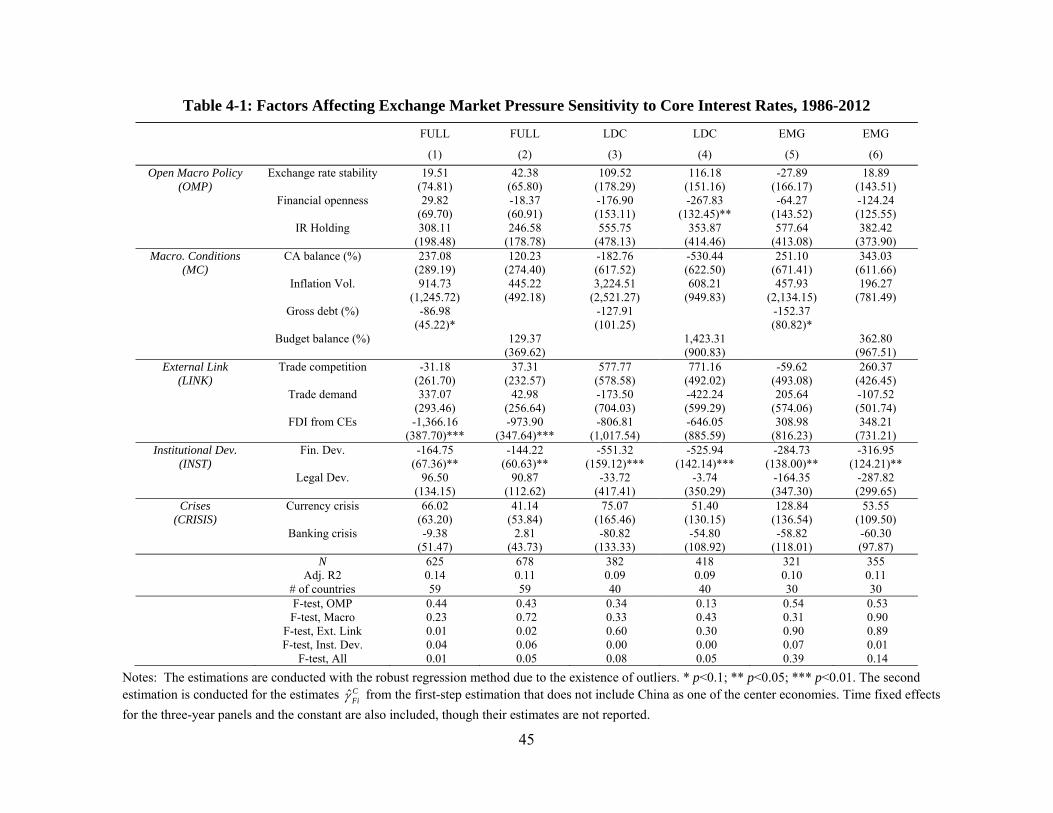
45  

Table 4-1: Factors Affecting Exchange Market Pressure Sensitivity to Core Interest Rates, 1986-2012

FULL FULL LDC LDC EMG EMG

(1) (2) (3) (4) (5) (6)

Open Macro Policy Exchange rate stability 19.51 42.38 109.52 116.18 -27.89 18.89 (OMP) (74.81) (65.80) (178.29) (151.16) (166.17) (143.51)

Financial openness 29.82 -18.37 -176.90 -267.83 -64.27 -124.24 (69.70) (60.91) (153.11) (132.45)** (143.52) (125.55) IR Holding 308.11 246.58 555.75 353.87 577.64 382.42 (198.48) (178.78) (478.13) (414.46) (413.08) (373.90)

Macro. Conditions CA balance (%) 237.08 120.23 -182.76 -530.44 251.10 343.03 (MC) (289.19) (274.40) (617.52) (622.50) (671.41) (611.66)

Inflation Vol. 914.73 445.22 3,224.51 608.21 457.93 196.27 (1,245.72) (492.18) (2,521.27) (949.83) (2,134.15) (781.49) Gross debt (%) -86.98 -127.91 -152.37 (45.22)* (101.25) (80.82)* Budget balance (%) 129.37 1,423.31 362.80 (369.62) (900.83) (967.51)

External Link Trade competition -31.18 37.31 577.77 771.16 -59.62 260.37 (LINK) (261.70) (232.57) (578.58) (492.02) (493.08) (426.45)

Trade demand 337.07 42.98 -173.50 -422.24 205.64 -107.52 (293.46) (256.64) (704.03) (599.29) (574.06) (501.74) FDI from CEs -1,366.16 -973.90 -806.81 -646.05 308.98 348.21 (387.70)*** (347.64)*** (1,017.54) (885.59) (816.23) (731.21)

Institutional Dev. Fin. Dev. -164.75 -144.22 -551.32 -525.94 -284.73 -316.95 (INST) (67.36)** (60.63)** (159.12)*** (142.14)*** (138.00)** (124.21)**

Legal Dev. 96.50 90.87 -33.72 -3.74 -164.35 -287.82 (134.15) (112.62) (417.41) (350.29) (347.30) (299.65)

Crises Currency crisis 66.02 41.14 75.07 51.40 128.84 53.55 (CRISIS) (63.20) (53.84) (165.46) (130.15) (136.54) (109.50)

Banking crisis -9.38 2.81 -80.82 -54.80 -58.82 -60.30 (51.47) (43.73) (133.33) (108.92) (118.01) (97.87) N 625 678 382 418 321 355 Adj. R2 0.14 0.11 0.09 0.09 0.10 0.11 # of countries 59 59 40 40 30 30 F-test, OMP 0.44 0.43 0.34 0.13 0.54 0.53 F-test, Macro 0.23 0.72 0.33 0.43 0.31 0.90 F-test, Ext. Link 0.01 0.02 0.60 0.30 0.90 0.89 F-test, Inst. Dev. 0.04 0.06 0.00 0.00 0.07 0.01 F-test, All 0.01 0.05 0.08 0.05 0.39 0.14

Notes: The estimations are conducted with the robust regression method due to the existence of outliers. * p<0.1; ** p<0.05; *** p<0.01. The second estimation is conducted for the estimates C

Fi from the first-step estimation that does not include China as one of the center economies. Time fixed effects

for the three-year panels and the constant are also included, though their estimates are not reported.

 

46  

Table 4-2: Factors Affecting Exchange Market Pressure Sensitivity to Core REER, 1986-2012

FULL FULL LDC LDC EMG EMG

(1) (2) (3) (4) (5) (6)

Open Macro Policy Exchange rate stability -4.296 -5.331 -1.954 -4.870 1.244 -2.477 (OMP) (3.269) (3.274) (3.291) (3.384) (4.044) (4.165)

Financial openness -9.415 -7.166 -7.360 -6.084 -8.324 -6.339 (3.046)*** (3.031)** (2.827)*** (2.965)** (3.493)** (3.644)* IR Holding -14.635 -15.171 -9.791 -10.705 -11.470 -12.454 (8.674)* (8.896)* (8.827) (9.279) (10.053) (10.852)

Macro. Conditions CA balance (%) -21.217 -16.464 -24.993 -15.372 -31.781 -20.494 (MC) (12.638)* (13.654) (11.400)** (13.936) (16.339)* (17.753)

Inflation Vol. 14.329 58.052 -2.863 73.630 13.702 80.103 (54.439) (24.490)** (46.546) (21.265)*** (51.937) (22.682)*** Gross debt (%) 1.207 -0.992 0.257 (1.976) (1.869) (1.967) Budget balance (%) -8.721 -14.180 -24.878 (18.392) (20.168) (28.082)

External Link Trade competition 16.175 16.889 16.344 17.914 13.900 15.391 (LINK) (11.437) (11.572) (10.681) (11.015) (12.000) (12.377)

Trade demand -14.134 -7.330 -25.070 -20.335 -33.885 -27.703 (12.824) (12.770) (12.997)* (13.417) (13.970)** (14.563)* FDI from CEs 20.388 17.320 23.582 21.515 34.115 32.611 (16.943) (17.298) (18.785) (19.826) (19.864)* (21.223)

Institutional Dev. Fin. Dev. -8.604 -8.868 -7.133 -6.044 -8.104 -6.107 (INST) (2.943)*** (3.017)*** (2.938)** (3.182)* (3.358)** (3.605)*

Legal Dev. 21.851 24.437 7.902 7.784 15.612 15.026 (5.862)*** (5.604)*** (7.706) (7.842) (8.452)* (8.697)*

Crises Currency crisis 7.238 7.495 7.464 8.885 6.067 6.188 (CRISIS) (2.762)*** (2.679)*** (3.055)** (2.914)*** (3.323)* (3.178)*

Banking crisis 5.694 7.428 2.254 3.863 7.808 9.125 (2.249)** (2.176)*** (2.461) (2.439) (2.872)*** (2.841)*** N 625 678 382 418 320 355 Adj. R2 0.15 0.18 0.12 0.18 0.14 0.19 # of countries 59 59 40 40 30 30 F-test, OMP 0.00 0.01 0.02 0.03 0.06 0.12 F-test, Macro 0.37 0.04 0.14 0.00 0.27 0.00 F-test, Ext. Link 0.31 0.35 0.19 0.26 0.10 0.20 F-test, Inst. Dev. 0.00 0.00 0.05 0.14 0.02 0.09 F-test, All 0.00 0.00 0.00 0.00 0.00 0.00

Notes: The estimations are conducted with the robust regression method due to the existence of outliers. * p<0.1; ** p<0.05; *** p<0.01. The second estimation is conducted for the estimates C

Fi from the first-step estimation that does not include China as one of the center economies. Time fixed effects

for the three-year panels and the constant are also included, though their estimates are not reported.

 

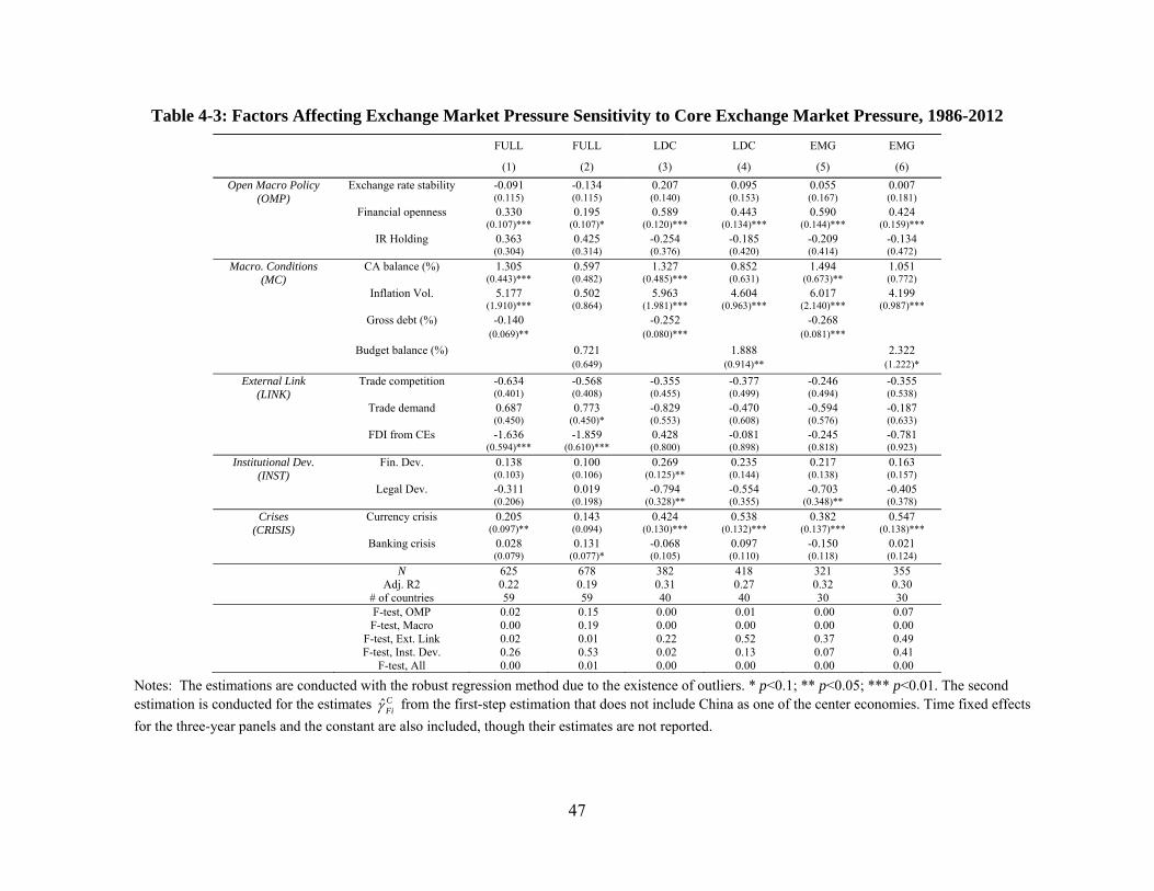
47  

Table 4-3: Factors Affecting Exchange Market Pressure Sensitivity to Core Exchange Market Pressure, 1986-2012

FULL FULL LDC LDC EMG EMG

(1) (2) (3) (4) (5) (6)

Open Macro Policy Exchange rate stability -0.091 -0.134 0.207 0.095 0.055 0.007(OMP) (0.115) (0.115) (0.140) (0.153) (0.167) (0.181)

Financial openness 0.330 0.195 0.589 0.443 0.590 0.424 (0.107)*** (0.107)* (0.120)*** (0.134)*** (0.144)*** (0.159)***

IR Holding 0.363 0.425 -0.254 -0.185 -0.209 -0.134 (0.304) (0.314) (0.376) (0.420) (0.414) (0.472)

Macro. Conditions CA balance (%) 1.305 0.597 1.327 0.852 1.494 1.051(MC) (0.443)*** (0.482) (0.485)*** (0.631) (0.673)** (0.772)

Inflation Vol. 5.177 0.502 5.963 4.604 6.017 4.199 (1.910)*** (0.864) (1.981)*** (0.963)*** (2.140)*** (0.987)***

Gross debt (%) -0.140 -0.252 -0.268 (0.069)** (0.080)*** (0.081)*** Budget balance (%) 0.721 1.888 2.322 (0.649) (0.914)** (1.222)*

External Link Trade competition -0.634 -0.568 -0.355 -0.377 -0.246 -0.355(LINK) (0.401) (0.408) (0.455) (0.499) (0.494) (0.538)

Trade demand 0.687 0.773 -0.829 -0.470 -0.594 -0.187 (0.450) (0.450)* (0.553) (0.608) (0.576) (0.633)

FDI from CEs -1.636 -1.859 0.428 -0.081 -0.245 -0.781 (0.594)*** (0.610)*** (0.800) (0.898) (0.818) (0.923)

Institutional Dev. Fin. Dev. 0.138 0.100 0.269 0.235 0.217 0.163(INST) (0.103) (0.106) (0.125)** (0.144) (0.138) (0.157)

Legal Dev. -0.311 0.019 -0.794 -0.554 -0.703 -0.405 (0.206) (0.198) (0.328)** (0.355) (0.348)** (0.378)

Crises Currency crisis 0.205 0.143 0.424 0.538 0.382 0.547(CRISIS) (0.097)** (0.094) (0.130)*** (0.132)*** (0.137)*** (0.138)***

Banking crisis 0.028 0.131 -0.068 0.097 -0.150 0.021 (0.079) (0.077)* (0.105) (0.110) (0.118) (0.124)

N 625 678 382 418 321 355 Adj. R2 0.22 0.19 0.31 0.27 0.32 0.30 # of countries 59 59 40 40 30 30 F-test, OMP 0.02 0.15 0.00 0.01 0.00 0.07 F-test, Macro 0.00 0.19 0.00 0.00 0.00 0.00 F-test, Ext. Link 0.02 0.01 0.22 0.52 0.37 0.49 F-test, Inst. Dev. 0.26 0.53 0.02 0.13 0.07 0.41 F-test, All 0.00 0.01 0.00 0.00 0.00 0.00

Notes: The estimations are conducted with the robust regression method due to the existence of outliers. * p<0.1; ** p<0.05; *** p<0.01. The second estimation is conducted for the estimates C

Fi from the first-step estimation that does not include China as one of the center economies. Time fixed effects

for the three-year panels and the constant are also included, though their estimates are not reported.

 

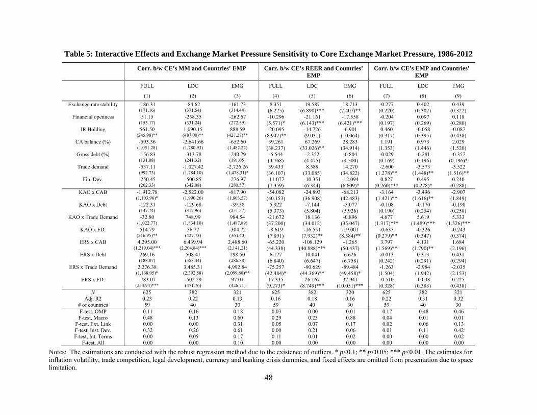
48  

Table 5: Interactive Effects and Exchange Market Pressure Sensitivity to Core Exchange Market Pressure, 1986-2012

Corr. b/w CE’s MM and Countries’ EMP Corr. b/w CE’s REER and Countries’ EMP

Corr. b/w CE’s EMP and Countries’ EMP

FULL LDC EMG FULL LDC EMG FULL LDC EMG

(1) (2) (3) (4) (5) (6) (7) (8) (9)

Exchange rate stability -186.31 -84.62 -161.73 8.351 19.587 18.713 -0.277 0.402 0.439 (171.16) (371.54) (314.44) (6.225) (6.890)*** (7.407)** (0.220) (0.302) (0.322)

Financial openness 51.15 -258.35 -262.67 -10.296 -21.161 -17.558 -0.204 0.097 0.118 (153.17) (331.24) (272.59) (5.571)* (6.143)*** (6.421)*** (0.197) (0.269) (0.280)

IR Holding 561.50 1,090.15 888.59 -20.095 -14.726 -6.901 0.460 -0.058 -0.087 (245.98)** (487.00)** (427.27)** (8.947)** (9.031) (10.064) (0.317) (0.395) (0.438)

CA balance (%) -593.36 -2,641.66 -652.60 59.261 67.269 28.283 1.191 0.973 2.029 (1,051.28) (1,780.93) (1,482.22) (38.237) (33.026)** (34.914) (1.353) (1.446) (1.520)

Gross debt (%) -156.83 -313.78 -240.79 -5.544 -2.352 -0.804 -0.029 -0.281 -0.357 (131.08) (241.32) (191.05) (4.768) (4.475) (4.500) (0.169) (0.196) (0.196)*

Trade demand -537.11 -1,027.42 -2,726.26 39.433 8.589 14.270 -2.600 -3.573 -3.522 (992.73) (1,784.10) (1,478.31)* (36.107) (33.085) (34.822) (1.278)** (1.448)** (1.516)**

Fin. Dev. -250.45 -500.85 -276.97 -11.077 -10.351 -12.094 0.827 0.495 0.240 (202.33) (342.08) (280.57) (7.359) (6.344) (6.609)* (0.260)*** (0.278)* (0.288)

KAO x CAB -1,912.78 -2,522.00 -817.90 -54.082 -24.893 -68.213 -3.164 -3.496 -2.907 (1,103.96)* (1,990.26) (1,803.57) (40.153) (36.908) (42.483) (1.421)** (1.616)** (1.849)

KAO x Debt -122.31 -129.68 -39.58 5.922 -7.144 -5.077 -0.108 -0.170 -0.198 (147.74) (312.96) (251.57) (5.373) (5.804) (5.926) (0.190) (0.254) (0.258)

KAO x Trade Demand -32.80 748.99 984.54 -21.672 18.136 -0.896 4.677 5.619 5.333 (1,022.77) (1,834.10) (1,487.89) (37.200) (34.012) (35.047) (1.317)*** (1.489)*** (1.526)***

KAO x FD. 514.79 56.77 -304.72 -8.619 -16.551 -19.001 -0.635 -0.326 -0.243 (216.95)** (427.73) (364.40) (7.891) (7.932)** (8.584)** (0.279)** (0.347) (0.374)

ERS x CAB 4,295.00 6,439.94 2,488.60 -65.220 -108.129 -1.265 3.797 4.131 1.684 (1,219.04)*** (2,204.84)*** (2,141.21) (44.338) (40.888)*** (50.437) (1.569)** (1.790)** (2.196)

ERS x Debt 269.16 508.41 298.50 6.127 10.041 6.626 -0.013 0.313 0.431 (188.07) (358.44) (286.88) (6.840) (6.647) (6.758) (0.242) (0.291) (0.294)

ERS x Trade Demand 2,276.38 3,485.31 4,992.84 -75.257 -90.629 -89.484 -1.263 -2.984 -2.035 (1,168.05)* (2,392.58) (2,099.68)** (42.484)* (44.369)** (49.458)* (1.504) (1.942) (2.153)

ERS x FD. -783.07 -502.29 97.01 17.335 26.167 32.941 -0.510 -0.038 0.225 (254.94)*** (471.76) (426.71) (9.273)* (8.749)*** (10.051)*** (0.328) (0.383) (0.438)

N 625 382 321 625 382 320 625 382 321 Adj. R2 0.23 0.22 0.13 0.16 0.18 0.16 0.22 0.31 0.32

# of countries 59 40 30 59 40 30 59 40 30 F-test, OMP 0.11 0.16 0.18 0.03 0.00 0.01 0.17 0.48 0.46 F-test, Macro 0.48 0.13 0.60 0.29 0.23 0.88 0.04 0.01 0.01

F-test, Ext. Link 0.00 0.00 0.31 0.05 0.07 0.17 0.02 0.06 0.13 F-test, Inst. Dev. 0.32 0.26 0.61 0.00 0.21 0.06 0.01 0.11 0.42 F-test, Int. Terms 0.00 0.05 0.17 0.11 0.01 0.02 0.00 0.00 0.02

F-test, All 0.00 0.00 0.10 0.00 0.00 0.00 0.00 0.00 0.00

Notes: The estimations are conducted with the robust regression method due to the existence of outliers. * p<0.1; ** p<0.05; *** p<0.01. The estimates for inflation volatility, trade competition, legal development, currency and banking crisis dummies, and fixed effects are omitted from presentation due to space limitation.

 

49  

Table 6: Interactive Effects for Developing Countries Conditional on KAOPEN and ERS

(a) Effect of CAB Deterioration (–2 ppt) in the MM-EMP Estimation

  KAOPEN   0.00  0.50  1.00 

ERS*  0.00  52.83 27.61 2.39

  0.50  -11.57 -36.79 -62.01

  1.00  -75.97 -101.19 -126.41

(b) Effect of Financial Development

(+10 ppt) in the REER-EMP Estimation

  KAOPEN*   0.00  0.50  1.00 

ERS* 0.00  -1.04 -1.86 -2.69

  0.50  0.27 -0.55 -1.38

  1.00  1.58 0.75 -0.07

(c) Effect of CAB Deterioration (–0.02 ppt) in the REER-EMP Estimation

  KAOPEN   0.00  0.50  1.00 

ERS* 0.00  -1.35 -1.10 -0.85

  0.50  -0.26 -0.02 0.23

  1.00  0.82 1.07 1.32

(d) Effect of Trade Demand (+5 ppt) in the REER-EMP Estimation

  KAOPEN   0.00  0.50  1.00 

ERS* 0.00  0.43 0.88 1.34

  0.50  -1.84 -1.38 -0.93

  1.00  -4.10 -3.65 -3.20

(e) Effect of CAB Deterioration (–2 ppt)

in the EMP-EMP Estimation

  KAOPEN*   0.00  0.50  1.00 

ERS* 0.00  -0.02 0.02 0.05

  0.50  -0.06 -0.03 0.01

  1.00  -0.10 -0.07 -0.03

(f) Effect of Trade Demand (+5 ppt) by the CE in the EMP-EMP Estimation

  KAOPEN*   0.00  0.50  1.00 

ERS 0.00  -0.18 -0.04 0.10

  0.50  -0.25 -0.11 0.03

  1.00  -0.33 -0.19 -0.05

Note: “*” superscripted to KAOPEN or ERS in the tables means that the interaction term between KAOPEN or ERS and the variable of concern is found to be statistically significant in each respective estimation.

 

50  

Figure 1: Correlations of the Short-Term Interest Rates with the United States

Figure 2: Correlations of the Long-Term Interest Rates with the U.S.

-1-.

50

.51

Cor

r. o

f ST

-int.

rate

s w

/ US

1990m1 1995m1 2000m1 2005m1 2010m1 2015m

IDC LDC EMEs

-1-.

50

.51

Cor

r. o

f LT

-int.

rate

s w

/ US

1990m1 1995m1 2000m1 2005m1 2010m1 2015

IDC LDCEMEs

 

51  

Figure 3: Correlations of the Stock Market Price Indexes with the U.S.

-.5

0.5

1C

orr.

of s

tock

mar

ket i

ndex

es w

ith th

e U

S S

&P

1990m1 1995m1 2000m1 2005m1 2010m1 2015

IDC LDCEMEs

 

52  

Figure 4: Proportion of Significant F-Tests

(a) Policy Interest Rate

(b) Stock Market Price Index

(c) Term spread

0.2

.4.6

.81

% o

f S

ig.

Est

imat

es

1992-19941995-1997

1998-20002001-2003

2004-20062007-2009

2010-2012

IDC Sample

Real Global Fin. GlobalCross-link Domestic

0.2

.4.6

.81

% o

f S

ig.

Est

imat

es

1992-19941995-1997

1998-20002001-2003

2004-20062007-2009

2010-2012

LDC Sample

Real Global Fin. GlobalCross-link Domestic

0.2

.4.6

.81

% o

f S

ig.

Est

imat

es

1992-19941995-1997

1998-20002001-2003

2004-20062007-2009

2010-2012

IDC Sample

Real Global Fin. GlobalCross-link Domestic

0.2

.4.6

.81

% o

f S

ig.

Est

imat

es

1992-19941995-1997

1998-20002001-2003

2004-20062007-2009

2010-2012

LDC Sample

Real Global Fin. GlobalCross-link Domestic

0.2

.4.6

.81

% o

f S

ig.

Est

imat

es

1992-19941995-1997

1998-20002001-2003

2004-20062007-2009

2010-2012

IDC Sample

Real Global Fin. GlobalCross-link Domestic

0.2

.4.6

.81

% o

f S

ig.

Est

imat

es

1992-19941995-1997

1998-20002001-2003

2004-20062007-2009

2010-2012

LDC Sample

Real Global Fin. GlobalCross-link Domestic

 

53  

Figure 4: continued (d) REER

0.2

.4.6

.81

% o

f S

ig.

Est

imat

es

1992-19941995-1997

1998-20002001-2003

2004-20062007-2009

2010-2012

IDC Sample

Real Global Fin. GlobalCross-link Domestic

0.2

.4.6

.81

% o

f S

ig.

Est

imat

es

1992-19941995-1997

1998-20002001-2003

2004-20062007-2009

2010-2012

LDC Sample

Real Global Fin. GlobalCross-link Domestic

 

54  

Figure 5: Proportion of Significant 0ˆ C Tests

0.2

.4.6

.81

% o

f Sig

. Est

imat

es

1992-19941995-1997

1998-20002001-2003

2004-20062007-2009

2010-2012

ST rate: LDC Sample

U.S. JapanEuro China

0.2

.4.6

.81

% o

f Sig

. Est

imat

es

1992-19941995-1997

1998-20002001-2003

2004-20062007-2009

2010-2012

Stock Market Index: LDC Sample

U.S. JapanEuro China

0.2

.4.6

.81

% o

f Sig

. Est

imat

es

1992-19941995-1997

1998-20002001-2003

2004-20062007-2009

2010-2012

Term Spread: LDC Sample

U.S. JapanEuro China

0.2

.4.6

.81

% o

f Sig

. Est

imat

es

1992-19941995-1997

1998-20002001-2003

2004-20062007-2009

2010-2012

REER: LDC Sample

U.S. JapanEuro China

 

55  

Figure 6: Contribution to Adjusted R2 of Adding China as a Center economy

0.0

5.1

.15

Add

ition

al c

ontr

. to

Adj

. R

2

1992-19941995-1997

1998-20002001-2003

2004-20062007-2009

2010-2012

ST Policy Rate

IDC LDCEMG E.Asian EMG

0.0

5.1

.15

Add

ition

al c

ontr

. to

Adj

. R

2

1992-19941995-1997

1998-20002001-2003

2004-20062007-2009

2010-2012

Stock Market Index

IDC LDCEMG E.Asian EMG

0.0

5.1

.15

Add

ition

al c

ontr

. to

Adj

. R

2

1992-19941995-1997

1998-20002001-2003

2004-20062007-2009

2010-2012

Term Spread

IDC LDCEMG E.Asian EMG

0.0

5.1

.15

Add

ition

al c

ontr

. to

Adj

. R

2

1992-19941995-1997

1998-20002001-2003

2004-20062007-2009

2010-2012

REER

IDC LDCEMG E.Asian EMG

 

56  

Figure 7: Exchange Rate, Interest Rate, and Real Money Stock of a Peripheral Country (PH) In Response to a Rise in the REER of the Center Economies (CE)

E

EER

e

CE

' 

E

EER

e

CE

 

1,PHR  0,PHR  

1

P

M 

0

P

M 

E0

E1

Exchange rate = price of CE’s currency in PH’s currency

PH’s Interest Rate

PH’s Real Money Stock

 

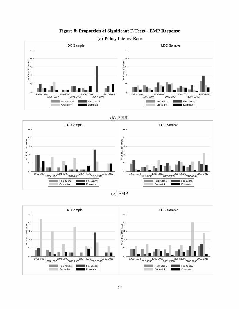
57  

Figure 8: Proportion of Significant F-Tests – EMP Response

(a) Policy Interest Rate

(b) REER

(c) EMP

0.2

.4.6

.81

% o

f S

ig.

Est

imat

es

1992-19941995-1997

1998-20002001-2003

2004-20062007-2009

2010-2012

IDC Sample

Real Global Fin. GlobalCross-link Domestic

0.2

.4.6

.81

% o

f S

ig.

Est

imat

es

1992-19941995-1997

1998-20002001-2003

2004-20062007-2009

2010-2012

LDC Sample

Real Global Fin. GlobalCross-link Domestic

0.2

.4.6

.81

% o

f S

ig.

Est

imat

es

1992-19941995-1997

1998-20002001-2003

2004-20062007-2009

2010-2012

IDC Sample

Real Global Fin. GlobalCross-link Domestic

0.2

.4.6

.81

% o

f S

ig.

Est

imat

es

1992-19941995-1997

1998-20002001-2003

2004-20062007-2009

2010-2012

LDC Sample

Real Global Fin. GlobalCross-link Domestic

0.2

.4.6

.81

% o

f S

ig.

Est

imat

es

1992-19941995-1997

1998-20002001-2003

2004-20062007-2009

2010-2012

IDC Sample

Real Global Fin. GlobalCross-link Domestic

0.2

.4.6

.81

% o

f S

ig.

Est

imat

es

1992-19941995-1997

1998-20002001-2003

2004-20062007-2009

2010-2012

LDC Sample

Real Global Fin. GlobalCross-link Domestic

 

58  

Figure 9: Proportion of Significant 0ˆ C or 0ˆ C Tests

(a) Policy Interest Rate ( 0ˆ C ) (b) REER ( 0ˆ C )

(c) EMP ( 0ˆ C ) (d) EMP ( 0ˆ C )

0.2

.4.6

.81

% o

f Sig

. Est

imat

es

1992-19941995-1997

1998-20002001-2003

2004-20062007-2009

2010-2012

ST rate: LDC Sample

U.S. JapanEuro

0.2

.4.6

.81

% o

f Sig

. Est

imat

es

1992-19941995-1997

1998-20002001-2003

2004-20062007-2009

2010-2012

REER: LDC Sample

U.S. JapanEuro

0.2

.4.6

.81

% o

f Sig

. Est

imat

es

1992-19941995-1997

1998-20002001-2003

2004-20062007-2009

2010-2012

EMP: LDC Sample

U.S. JapanEuro

0.2

.4.6

.81

% o

f Sig

. Est

imat

es

1992-19941995-1997

1998-20002001-2003

2004-20062007-2009

2010-2012

EMP: LDC Sample

U.S. JapanEuro