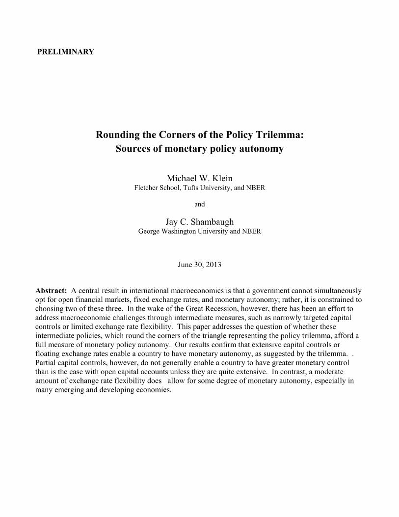
PRELIMINARY

Rounding the Corners of the Policy Trilemma: Sources of monetary policy autonomy

Michael W. Klein Fletcher School, Tufts University, and NBER

and

Jay C. Shambaugh George Washington University and NBER

June 30, 2013

Abstract: A central result in international macroeconomics is that a government cannot simultaneously opt for open financial markets, fixed exchange rates, and monetary autonomy; rather, it is constrained to choosing two of these three. In the wake of the Great Recession, however, there has been an effort to address macroeconomic challenges through intermediate measures, such as narrowly targeted capital controls or limited exchange rate flexibility. This paper addresses the question of whether these intermediate policies, which round the corners of the triangle representing the policy trilemma, afford a full measure of monetary policy autonomy. Our results confirm that extensive capital controls or floating exchange rates enable a country to have monetary autonomy, as suggested by the trilemma. . Partial capital controls, however, do not generally enable a country to have greater monetary control than is the case with open capital accounts unless they are quite extensive. In contrast, a moderate amount of exchange rate flexibility does allow for some degree of monetary autonomy, especially in many emerging and developing economies.

1  

I. Introduction:1

Policy makers cannot have it all, at least in the sphere of international macroeconomics. This is

the idea behind the policy trilemma, a central principle of international macroeconomics that maintains

that a country can maintain only two of three policies; a fixed exchange rate, open capital markets, and

domestic monetary autonomy. The reason is fairly straightforward. If a country has a fixed exchange

rate and open financial markets, its interest rate must follow that of the base country, which implies

sacrificing monetary autonomy. Otherwise, for example, an increase in the base country interest rate not

matched by the domestic country would lead to investors shifting funds to assets denominated in the

higher interest rate currency, which generates a depreciation of the exchange rate. Thus, monetary

autonomy requires that a country must either allow the exchange rate to change or shut down the flow of

finance across borders.

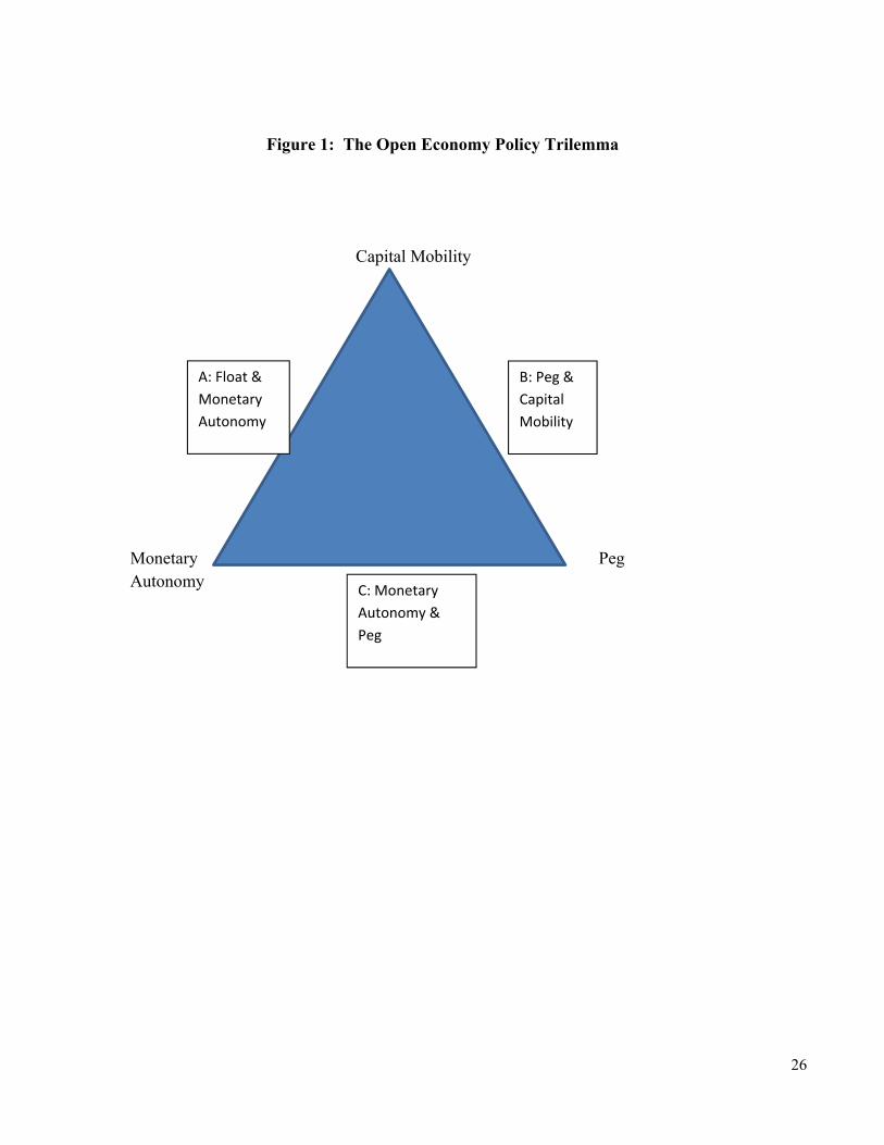
The policy trilemma is often depicted using the diagram presented in Figure 1. Each of the

corners of the triangle represents one of the three policy choices. A government can choose a position

represented by one of the sides of the triangle: a floating exchange rate with monetary autonomy and

capital mobility (side A); a pegged exchange rate with capital mobility but no monetary autonomy (side

B); or monetary autonomy and a pegged exchange rate, but with capital controls (point C). While a

strict interpretation of the trilemma means that countries are forced to one of these sides, a more

tempered view is that the trilemma simply highlights tradeoffs; if financial markets are open, more

autonomy requires more exchange rate flexibility or, conversely, if the exchange rate is to remain stable,

more autonomy would require a more closed capital market.

The policy trilemma has been subjected to extensive empirical testing over the last decade. Early

results (Shambaugh (2004), Obstfeld et al (2005)) established the validity of the framework. These

results countered the notion that countries broadly lacked monetary autonomy, or that there was little

difference in monetary autonomy that could be obtained under different exchange rate regimes.

Subsequent work supports the relevance of the trilemma. Bluedorn and Bowdler (2010) demonstrate

that it holds for identified monetary policy shocks in the base country, not just for actual interest rate

movements. Miniane and Rogers (2007) confirm that interest rates in countries that peg follow the

interest rate of their base country more closely than do the interest rates of countries that float, but they

                                                            1 We thank Maury Obstfeld, Linda Goldberg, Olivier Jeanne, and participants at seminars at American University, Johns Hopkins University, London Business School, Queens College (Belfast), Trinity University (Dublin), and ETH (Zurich) for comments. We also thank the organizers, participants, and in particular our discussant Keen Meng Choy at the Bank of Japan’s International Monetary and Economic Studies conference. We thank Anthony Trifero and Patrick O’Halloran for research assistance and Hiro Ito, Menzie Chinn, and Bilge Erten for sharing data.

2  

do not find significant differences across their capital control regime categories. Aizenmann et al (2010)

show that, in this context, movements in one policy requires corresponding changes in another policy;

for example, more restricted capital flows enable a country to have either more monetary autonomy or

greater control over its exchange rate.

A common result in the literature, one that we find as well, is that open pegs broadly follow the

base country interest rate and closed non-pegs do not. But the focus of this paper is to go beyond this

point by analyzing the extent to which monetary policy autonomy can be achieved through limited

capital market intervention, or through allowing the exchange rate to fluctuate within a narrow band,

two sets of policies that have gained greater attention since the onset of the global financial and

economic crisis. .

The international policy making community had been somewhat skeptical about the wisdom of

using capital controls to generate autonomy in the pre-crisis period. In the wake of the crisis, however,

there has been a re-evaluation of the desirability of capital controls, especially those restrictions that are

imposed episodically at times of incipient inflow surges. In a notable reversal from their earlier stance,

the IMF has suggested capital controls may be warranted under certain conditions (see Ostry et al,

2012). Theoretical work offers a view that targeted capital controls, used in a flexible manner, could

serve a prudential role and reduce financial fragility (Jeane (2011, 2012), Jeanne and Korinek (2010),

Korinek (2011), Bianchi (2011)) or, for pegged countries could substitute for monetary policy autonomy

and provide a pegged country some control over macro policy management (Farhi and Werning (2012)

and Schmitt-Grohe and Uribe (2012)).

One facet of this paper is to empirically investigate whether limited capital controls temper the

loss of monetary policy autonomy that accompanies pegged exchange rates. An important point is the

possible distinction between episodic, targeted capital controls and long-standing controls over a wide

range of assets. Another facet of this paper is to study whether an intermediate exchange rate regime, a

“soft” peg in which an exchange rate is allowed to fluctuate within relatively wide bands, affords more

monetary autonomy than a peg in which the domestic currency is more tightly aligned with the value of

the currency of a base country.

We consider each of these two facets of middle-ground policies, and the possibility of rounding

the corners of the policy trilemma, along the dimensions of time and policy intensity. Middle-ground

policies arise in the time dimension through blended behavior across years, such as opening and closing

3  

the financial account, or flipping back and forth across exchange rate regimes. Policy middle grounds in

a particular year are represented by loose pegs and limited capital controls.

These two ways in which the corners of the policy trilemma can be rounded, by switching

policies over time and by mid-range policies, are relevant for both exchange rate and capital control

regimes. While there are some cases of movement towards “bipoloar” exchange rate regimes, as

suggested by Fischer more than a decade ago and as exemplified by the move from the EMS bands to a

single currency in the euro-zone, there remains an important and empirically relevant middle ground

between long-standing pure pegs and floats. One aspect of this is the continued presence of “soft” pegs.

Another is the flipping back and forth between pegs and floats (Klein and Shambaugh (2008).

Likewise, there are empirically relevant middle ground policies with respect to capital controls. While

some countries have long-standing, pervasive capital controls, there is a substantial subset of countries

that use limited controls on an episodic basis. Klein (2012) calls these capital control regimes “walls”

and “gates,” respectively, and shows that Klein (2012)walls are more effective than gates in limiting

asset price booms and swings in the value of the real exchange rate.

In this paper, we also find differences in the effects of gates and walls, and that the sharp

trilemma corner representing capital account openness cannot be rounded by using temporary capital

controls unless they are quite extensive. Similarly, flipping exchange rate regimes does not change the

general nature of the trilemma. When countries are pegged, they move with the base, when not pegged,

they do not. Thus a temporary float does seem to generate autonomy and a temporary peg sacrifices it.

However, soft pegs do seem to generate more monetary policy autonomy than tight pegs, even though

they do not afford as much autonomy as floating exchange rates.

On net, then, the results presented in this paper confirm the basic message of the trilemma; pegs

and open countries have less monetary autonomy, and efforts to gain autonomy through middle range

policies may be difficult. The most simple and most sure way to get monetary autonomy, without

strongly closing off the capital account, is to allow more flexibility in the exchange rate.

II. Methodology

The key question in this paper is how a country can achieve monetary autonomy, in particular

the extent to which the trade-offs represented by the policy trilemma are materially altered by allowing

some exchange rate flexibility, or by using capital controls episodically. An answer to this question

sharpens our understanding of the policy trilemma. It is not the case, however, that the trilemma is

4  

refuted by results showing a degree of monetary autonomy is obtained with soft pegs rather than just

with pegs, or with gates rather than walls. The trilemma does not require that countries only occupy

corner solutions, rather it is an expression of the trade-offs faced by policy-makers. To answer this

question we follow the techniques used in Shambaugh (2004) and Obstfeld et al. (2005). The core

methodology in this paper is straightforward. It begins from the simple interest parity equation

(1) Rit = Rbit + %ΔEe + ρ

where R represents the nominal interest rate, Rb is the interest rate of the base country, %ΔEe is the

expected change in the exchange rate and ρ represents the risk premium on the asset in question.

Under a purely credible peg with a perfectly fixed exchange rate, the expected change in the

exchange rate is zero. If the assets in question have similar risk (and they are either short term money

markets or short term government bonds which should have relatively low risk premia), then the local

interest rate must equal the base-country interest rate. In the case of nonpegs, however, the local interest

rate could differ from the base-country rate.

In addition, the equation should only hold if money can flow across borders to enforce it. If

capital controls are tight,there is no reason Rit must equal Rbit regardless of %ΔEe, Alternatively, we

could think about capital controls as a wedge between Rit and Rbit . For example, if there were a tax on

foreign borrowing and there were net inflows (so the marginal capital came from abroad) we could

rewrite (1) as:

(2) Rit = Rbit + %ΔEe + ρ+ τ

where τ represents the tax. Thus, by raising or lowering τ, the government could have Rit move

differently from Rbit even if %ΔEe is equal to zero, effectively giving the country monetary autonomy.

This, in principle, is the monetary autonomy Farhi and Werning (2012) or Schmitt Grohe and Uribe

(2012) have in mind.2

One complication is that we do not directly observe the expected change in the exchange rate or

the risk premium. Interest rates may not be equal, even in the case of pegged exchange rates, because of

movements in these variables. Furthermore, there is extensive research showing that this basic equation

does not hold for nonpegs when one uses the realized ex post exchange rate change as a proxy for the ex                                                             2 Schmitt-Grohe and Uribe state: “As a result, the government can indirectly affect employment in the nontraded sector by manipulating the intertermporal price of tradables (the interest rate) via capital controls.” It should be noted, Schmitt-Grohe and Uribe do not suggest this is a first best policy. They suggest allowing the exchange rate to change is preferable, but study the question of what should be done if that tool is not available. Farhi and Werning, argue: “In response to transitory shocks, however, capital controls now play a more important countercyclical role” when prices are sticky, and “This discussion underscores the fact that capital controls allow the country to regain some monetary autonomy and, with it, some control over the intertemporal allocation of spending.” 

5  

ante expected change. But, as long as %ΔEe + ρ do not move systematically with the base interest rate

(which would be true, for example if the peg was fully credible and the risk premium was constant), the

estimates should show that the change in the local interest rate moves with the change in the base

interest rate. Therefore, one set of our empirical tests centers on

(3) ΔRit = α + βΔRbit + µit

The coefficient of interest in this equation is β. If the trilemma held perfectly, we would expect β to be

equal to 1 for purely open pegs. Put differently, if equation (1) holds, ρ and %ΔEe are constant, and the

country does not try to move Rit on its own, then β will equal 1. Thus, we will use the estimated β as a

measure for countries’ monetary autonomy. If ρ and %ΔEe are not constant, then β will equal

(4) 1 ,%

Thus, if Rbit and %ΔEe or ρ are negatively correlated, then β will be less than one, and if positively

correlated, it will be less than one, even if there is no autonomy. On the other hand, transaction costs and

small barriers to arbitrage may allow for slight changes in the interest rates such that β is less than 1.

Obstfeld et al (2005) also demonstrate through simulations that as long as a country is allowed a small

amount of exchange rate flexibility within a band, the estimated β in such an equation could be closer to

0.5. We can also learn about the extent of autonomy in a particular sample of countries by the R-

squared in such an equation. A high R-squared shows that little else drives the local interest rate other

than the base interest rate. A low R-squared shows that many other factors may drive the local interest

rate. Again, Obstfeld et al (2005) provide a benchmark for the R-squared suggesting that even a country

following the base country quite closely in a credible peg with tight bands will still likely generate an R-

squared of only 0.1 or 0.2.

The specification that uses first differences, (3), has the additional advantage of accounting for

the fact that nominal interest rates exhibit substantial persistence and may be best treated as very close to

a unit root. Shambaugh (2004) discusses the time series properties of the data in detail.3 Our tests use

annual data, which enables us to abstract from slightly different adjustment speeds across countries so

                                                            3 One can estimate levels relationships and test the long run relationship and speed of adjustment and use critical values that vary depending on the unit root properties of the data (see Shambaugh (2004) and Frankel et al (2005)), but doing so requires fairly long samples with the same properties. As we want to focus on shifts across exchange rate and capital controls regimes, it is difficult to find long enough episodes to use these techniques.

6  

we can pool data. Accordingly, both the exchange rate regime and capital control regime data are also

coded at the annual frequency.

In practice, we will run separate regressions for subsamples of the data, corresponding to

different combinations of exchange rate regime and capital controls, and compare βs and R² across these

categories. For example, if we divided the sample along the dimensions of floats vs. pegs and open

capital markets vs. closed capital markets, we would have four categories; floats with open capital

markets, pegs with open capital markets, floats with closed capital markets and pegs with closed capital

markets. In this case, we expect to have the larger βs and higher R²s for the set of pegs as compared to

the set of floats, and for the set of open capital accounts as compared to the set of closed capital

accounts.

We can test for the statistical significance across these samples by pooling the data and using a

regression that interacts the change in the base interest rate with the exchange rate regime and an

indicator of capital account controls. In the case of peg vs. nonpeg (P = 1 for peg, P = 0 for nonpeg), the

equation would be:

(5) ΔRit = α + βRΔRbit + βRPPitΔRbit µit .

In this case, the effect of a change in the base country interest rate on the local interest rate is βR for a

nonpegged country and, βR + βRP for a peg. We can test βRP to see if there is a statistically significant

gap in the β across pegs and nonpegs. We expect βRP to be positive (the domestic interest rate follows

the base interest rate more closely when the country pegs). This equation can be augmented with other

interactions – in particular measures of a country’s capital control regime. It is straightforward to extend

this specification to three categories of capital controls (e.g. walls, gates and open) and/or three

categories of exchange rate regimes (peg, soft peg, and float).

One disadvantage of the interaction technique is that if βR is well estimated in one sub-sample

(e.g. pegs) but is noisily estimated in the other (floats), when data is pooled, βRP may be estimated with

large errors. In this particular circumstance, we have a strong prediction for what β is for the open

pegged countries, but in theory, there is no constraint on the monetary policy of the closed or floating

countries. If some countries move their interest rates sharply, and sometimes in the same direction of

the base country, pooling the data may show a fair bit of volatility.

At a conceptual level, the danger in such tests is that countries are moving their interest rates

together for reasons other than the constraints of the trilemma. If all countries are the same, comparing

pegs and floats would still be an effective method. But, if for some reason, pegs are more apt to make

7  

the same interest rate changes as the base country, our methodology will overstate the influence of

pegging. Shambaugh (2004) provides a number of tests looking at trade shares and other reasons a

country may follow the base and finds that the core results still hold. The capital control results are in

some ways insulated from this bias because it biases against the results. That is, if a country imposes

capital controls to avoid having to move with the base when there is pressure to do so, we would expect

it to appear to still follow the base to some extent relative to a non-capital control observation that faced

no such pressure. Given that the result is that capital controls insulate the local country, this potential

issue does not appear to be too problematic.

A number of other controls could be included in the regression. For example, country fixed

effects could be included, but these are effectively meaningless as to be anything other than zero, would

suggest a country is constantly raising its interest rate (if positive) or lowering it (if negative). One

could also include year fixed effects, and this would be a way to remove any global shock to interest

rates. Many papers that examine the trilemma do not do so because they use only one base country

which would be collinear with a time fixed effect. If there are multiple bases, though, and if the base

country interest rates are not correlated, this would provide the necessary variation. However, this

approach also removes a fair bit of information. To the extent that many countries follow the US dollar,

many observations are tied to the U.S. interest rates. In that case, a time fixed effect – estimated across

the average of the sample – will remove much of the movement from the dollar interest rate. Thus, in a

small sample, with a limited number of bases, time fixed effects may be problematic. Throughout the

paper, we report the version without year fixed effects, but we also occasionally note the year fixed

effect results (and include some tables with year fixed effects in the appendix). The core results of the

paper are not altered by year fixed effects, but it does make interpreting R-squared difficult across

samples.

III. Data

A crucial aspect of any test of the trilemma is identifying the indicators of monetary policy,

exchange rate regime and capital controls that can be used to test how closely the interest rate of a

country follows the interest rate of the base country. In this section we discuss the indicators we use,

and present some statistics.

8  

The core measure of a fixed exchange rate is derived from Shambaugh (2004) and is extended

here to a longer sample.4 This measure codes a country as pegged if its exchange rate stays within a +/-

2% band over the course of a year against its base country. The choice of the band width is based on the

fact that over time, ranging from the arbitrage bands of the gold standard to Bretton Woods, to the EMS,

bands of roughly 2% have often been allowed in fixed exchange rate systems. The base country is

identified based on the declared intent of the country, a country’s history, and by testing against a

variety of base countries. Countries are also considered pegged if their exchange rate is constant in 11

of twelve months but has a discrete devaluation or revaluation in the other month of the year. To avoid

misclassifying a country that simply has low volatility in a given year, single year pegs are not included

as pegs. Inspection of the observations of pegs shows no examples of countries that appear to be

spuriously coded as pegged due to lack of volatility.

We do not use the simple declaration by countries as to whether they are pegged or not since, as

is well documented in the literature, countries often do not accurately declare their exchange rate

regimes. Other classifications are available as well, but as we would like to isolate different aspects of

the policy trilemma, we prefer this measure which focuses solely on the exchange rate behavior. Klein

and Shambaugh (2010) document that this classification scheme has a reasonably high correlation with

both de jure and other de facto classifications.5 In addition to these pegs, we also consider a category of

“soft”pegs, as in Obstfeld et al. (2010). An exchange rate is classified as a soft peg if it is not a peg and

if the bilateral exchange rate with the base country stays within a range of up to +/-5% in a given year or

has no month where the exchange rate changed by more than 2% up or down (as a practical matter,

almost no countries qualify for the second criterion that fail to meet the first). As with the peg

classification, countries may not be considered a float in both the year prior to and following the

observation for the coding to count it as a soft peg.6 This is intended to reduce the odds of spuriously

coding countries as soft pegs. For example, the United States would never be coded as a soft peg

against Germany, as it never stays within a +/-5% band for more than one year at a time. Henceforth,

                                                            4 See Klein and Shambaugh (2010) for an extensive discussion of the coding of exchange rate regimes, and the different types of classifications that have been used. 5 Regarding two other popular choices, the Reinhart Rogoff classification codes countries as pegged if the black market exchange rate is stable, but that in some sense mixes two aspects of the trilemma – financial controls and exchange rate stability. Thus, for the purposes of examining the trilemma, it seems a pure focus on the exchange rate is more appropriate. Similarly, Levy Yeyati and Sturzennegar use data on reserves volatility to see if a country is intervening to maintain its peg. But, the index subsequently must add other pegs that do not intervene but that are clearly low volatility options. Furthermore due to the greater data needs, the index is available for a smaller sample of observations. 6 Countries do not have to be a soft peg for two years in a row, since a country could move from a peg to a soft peg or from a soft peg to a peg. Only soft pegs that are bordered on either side by a float are considered spurious.

9  

we will use the phrase peg to refer to a peg within 2% bands, a soft peg as one within 5% up or down

bands, and a float as a country that is neither. When looking simply at the binary coding we will refer to

pegs and nonpegs where nonpegs are both floats and soft pegs.

Table 1A presents the statistics on the exchange rate regime for the two data sets used in the

analyses in this paper, the 1973 – 2011 data and the shorter 1995 – 2011 data (The data sets correspond

to the two different capital control measures discussed below. The shorter data set covers fewer

countries than the longer data set.) In the Gates and Walls data set, there is a roughly even division

across the three exchange rate regime categories of peg, soft peg, and floating. The longer data set has a

relatively higher proportion of pegs, a relatively lower proportion of soft pegs, and a slightly smaller

proportion of floating exchange rate observations. But, this difference is not one related to time period

but country coverage. There is almost no difference in the peg / soft peg / float division in the full

sample or in the post 1995 sample. Thus, the middle ground appears sufficiently occupied to warrant

investigation.7

Classifying capital control regimes is more difficult than classifying exchange rate regime. One

can choose either a de jure or de facto means of classifying exchange rate regimes but capital controls

can only be gauged using de jure measures since there is a general absence of data on gross capital flows

and, even if these data were available, it is not clear what the level of gross flows would be in the case of

free capital mobility. It would be difficult to determine the extent of de facto controls by considering

whether rates of return are equalized across countries since this assumes efficient markets, knowledge of

investors’ expectations of the future value of the exchange rate, information on investor preferences and

correlations of returns with other measures of risk. Thus, researchers tend to use de jure measures of the

countries’ laws and regulations concerning financial flows. A disadvantage of any coding that relies on

laws or administrative rules as opposed to their application is it will be unable to measure intensity of

rules or of their implementation (for example, a 1% tax is a tax just as a 20% tax is and either would be

coded as a control).

The most consistent source of cross-country data on capital controls is the Annual Report on

Exchange Arrangements and Exchange Restrictions (AREAER) published by the IMF. Up until 1995,

this yearbook presented binary codes across a limited number of fields (controls on current account

                                                            7 See also Popper et al (2012) and Williamson (2000) among other studies for a discussion of the fact that the middle ground does appear occupied. It is worth noting that even conventional pegs differ from the hard pegs (e.g. currency unions and currency boards) that Fischer suggested would be the logical endpoints. Roughly half of the pegs are not purepegs but have some movement within the 2% bands.

10  

transactions, capital account transactions, multiple exchange rates, etc.). The level of detail was

expanded dramatically in the 1995 yearbook which began to report separate indicators of controls on

money market instruments (debt instruments with a maturity of less than 1 year), bonds (debt

instruments with a maturity of greater than one year), financial investments (which includes bank

borrowing and lending), collective investments, equities, and direct investment. Also, for the first time,

separate indicators were included for regulations on inflows and outflows for each of these categories.8

We use two sets of indicators of capital controls in this paper, both of which draw on the

AREAER. The Chinn-Ito index (created in Chinn and Ito (2006)) takes the first principal component of

the IMF AREAER yearbook coding of controls relating to current or capital account transactions, the

existence of multiple exchange rates, and the requirements of surrendering export proceeds. This index

covers a wide set of countries over a long time period, allowing for tests on a large sample of data. The

annual Chinn-Ito data we use in this paper covers the 1973 to 2011 period. This classification allows for

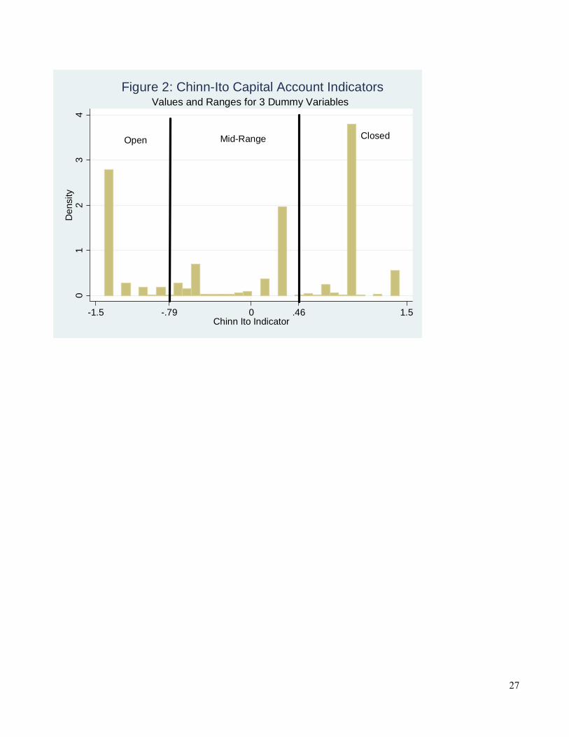
a country to be in different categories across time. As shown in Figure 2, these data are close to tri-

modal, so we use these data to create three dummy variables, one for open capital accounts, one for

closed capital accounts, and a third for an intermediate level of openness.9

The second set of capital control indicators use information from the post-1995 volumes of the

AREAER in a manner that builds on Schindler (2009).10 We follow the strategy of Klein (2012) who

distinguishes between countries that persistently had open capital accounts (“open”), countries that

persistently had closed capital accounts (“walls”), and countries that used capital controls episodically

(“gates”); thus, unlike the Chinn-Ito data, in this scheme a country does not change categories across

time.11 This division of countries into the three categories is based on the information from the AREAER

for five categories of financial flows (all but direct investment) for both inflows and outflows. As

discussed in Klein (2012), there is a relatively straightforward separation of countries into these three

                                                            8 We focus on the ten indicators signifying controls on inflows or outflows in the categories other than direct investment. Direct investment controls can be associated with intellectual property rules, national security, or many other features separate from controlling the flow of finance. Because the indicators are highly correlated (especially for walls countries that effectively have controls on all indicators), we focus on the gates / walls distinction, not fine variation across the different indicators. 9 Comparing these cuts in the index to the old binary coding of the IMF yearbook (for the years where available), we found that the open countries were always open according to the yearbook, the closed countries were always closed, and those that are in the middle ground based on the Chinn-Ito index were sometimes coded as open and sometimes coded as closed. 10 We thank Bilge Erten, who extended the country coverage of the Klein (2012) data set and kindly shared her data with us. 11 In the three way coding based on the Chinn Ito index, 87 of the 134 countries change capital control status with 66 making moves in the direction of more openness, and 56 making moves in the direction of being more closed. Some countries moved back and forth, and some countries moved more than once (for example, in two steps from completely closed to completely open) generating a total of 159 moves in capital account status based on our three way coding.

11  

categories since capital controls were imposed for long duration and over a majority of categories for

“walls” countries, while there were almost entirely absent for the countries in the open category. For the

walls countries, the average value of the ten categories (where 1 signifies a restriction and 0 represents

no restriction) is .93. That is, these countries are almost entirely closed in every year. Conversely, the

open countries have an average value of .02, suggesting most never have even a single restriction noted.

For the countries in the gates category, the average value for the 0/1 indicators is .43. We

distinguish between years in which the capital account was closed in any way and those in which it was

open. Open gates are those that have no restrictions (and hence an average value of zero); closed are

those that have any restriction at all (average value of .54). Thus, while the open gates look very much

like the open countries in general (in that there are no restrictions), closed gates are somewhat different

from walls. In addition to not being long lasting, they are not as extensive even when closed. We

sometimes divide the closed gates into “narrow” gates, which equals 1 in years in which represents the

average of the number of closed categories was greater than zero and equal to or less than 0.49 (that is,

fewer than half of the 10 categories are closed, average value .26), and “broad” gates, which equals 1 in

in years in which this average is greater than 0.49 (meaning at least half of the categories show a

restriction, average value .77). These broad gates are more similar to walls in their coverage of assets,

though given their temporary nature, they still may be more permeable.

Table 1B reports the number of observations in each category for each classification scheme.

The statistics in this panel show that the Chinn-Ito (CI) classification allows for a country to be in

different categories across time. This classification puts 38% of the 1973 – 2011 observations in the

closed category, 31% in the mid-range of capital controls category, and 31% in the open category. The

Gates-Walls-Open (GWO) classification divides the data by country, not by country-year observation.

It places the most observations in the gates category (48%), the next most in the open category (29%),

with the remaining 23% in the closed category. Of those 610 gates country year observations, 123

represent years in which there are no controls in place and 487 have some type of controls on asset

trade.. These closed gates observations are roughly evenly split between broad gates and narrow gates

(272 broad and 215 narrow).

Table 1C compares the Chinn-Ito (CI) and Gates/Walls/Open (GWO) indicators. This table

shows that the vast majority of observations coded as open in GWO are also coded as open in CI. Most

of the GWO walls observations are in the closed CI category (with some in the mid-range). Effectively

all the GWO open gates are coded as open by CI, and the closed gates are spread across all three

12  

categories. The narrowly targeted closed gates are predominantly open and middle (though some are

closed) and the broad closed gates are predominantly middle and closed (though some are open).

These statistics show that there is an empirically relevant number of observations that are not the

polar cases of float and peg, or fully open and fully closed capital accounts. We next turn to the

question of whether these middle ground policies allow for more monetary autonomy than a peg, or than

a fully open capital account.12

IV. Results

This section presents results for both a data set using the Chinn-Ito capital control data, which

covers the period 1973 – 2011, and one using the gates, walls, and open division of countries, which

covers the period 1995 – 2011.

IV.1 Core evidence on the Trilemma

Table 2 presents subsample regressions using the longer (Chinn-Ito) data set running regressions

with the specification presented in equation 3. In the first binary split of the data, we isolate pegs from

all other countries (grouping soft pegs and floats together) and isolate open countries from those with

any controls (middle closed or closed capital markets). Each of the four panels of table 2 represents one

of the archetypal options that the trilemma presents: open pegs, open nonpegs, closed pegs, and closed

nonpegs. Each panel shows the β coefficient (that on the base interest rate) as well as the standard error,

the number of observations and the R2.

For open financial market pegs sample, the coefficient is 0.68 (and the base interest rate

movements explain 28% of local country interest rate movements).13 Alternatively, the coefficient in

                                                            12 The other data used in the analysis (interest rates, reserves, etc) are from standard sources and are described in the data appendix. The data set is an unbalanced panel based on data availability for exchange rates, interest rates, and capital control data. Regressions using the Chinn-Ito data set are limited to 3126 observations across 134 countries. The only limitation other than data availability is that the United States is not included as it has no logical base country (any correlation between the US and another country’s interest rate is presumed to be the other country following the US). In addition, large swings in local interest rates are excluded since, in a handful of extreme cases, rates change by over 900 percentage points in a year and these observations would dominate the results. Leaving out changes of 50 percentage points or more represents roughly 1% of the observations, leaving out changes of 9 percentage points represents roughly 5% of the observations. In small samples, large but not extreme changes (between 9 and 50 percentage points) can also be large enough for one observation to dominate the estimates. We thus use the 9 percentage point cutoff for our baseline results. All main results are consistent if using the 50 percentage point change cutoff. Two other possible restrictions – dropping very small countries or dropping countries with clearly non market interest rates (ones that do not change for multiple years) – tend to strengthen the results, but these results are not reported. 13 Standard errors are clustered at the country level so as to allow for an unstructured covariance matrix within a set of observations for a country (controlling for serial correlation in the panel as well as the possibility of different size errors

13  

the closed pegs sample is 0.40, also highly statistically significantly different from zero, but the R-

squared is only half the size. Thus, despite the closed financial markets, these pegs still move in

conjunction with the base interest rate. Interest rates in open float countries are also not completely

uncorrelated with those of the base countries. The coefficient in this group is 0.23 and is statistically

significantly different from zero.14 Finally, interest rates in the closed nonpegs countries show almost

no relationship with the base countries’ interest rate. The coefficient is close to zero (.09), though it is

statistically different from zero at the 90 percent confidence level. Figure 3 (panels a-d) highlight these

results. It shows scatter plots of these subsamples. Open pegs appear to move quite closely with the

base country while closed pegs and open nonpegs move somewhat with the base. The picture for the

closed nonpegs shows almost no relationship at all.

One way of seeing if pegs truly follow the base or are just more likely to move with major

country interest rates is to look at how they respond to interest rate changes other than that of their base

country. If one looks at the non-dollar based sample, pegs and nonpegs respond quite differently to their

base interest rate – with pegs far more correlated with the base – but they respond nearly identically to

changes in the US dollar interest rate.15 To make comparisons across groups easier, we use the

specification in equation (5) and include interaction terms. These results are reported in the marginal

column and row of Table 2. The coefficient on pegs versus nonpegs is .33 and the coefficient on open

versus closed is .27. Both are statistically significantly different from zero at the 99 percent confidence

level.16 These results are quite similar to those in Shambaugh (2004) or Obstfeld et al (2005), even

though these results include ten more years of data.

One notable result is that while the trilemma predicts that an open financial market float or

closed financial market peg have autonomy -- only an open peg does not – the results show significant

coefficients for both of the off diagonals of the grid. Both being open and pegging seems to cost

monetary autonomy and giving up either one does not in and of itself gain pure autonomy. These results

are consistent with those in Obstfeld et al (2005) and Bluedorn and Bowdler (2010) but suggest that a

                                                                                                                                                                                                              across countries). One could alternatively control for correlation within a given year across countries, the standard errors are nearly identical across the two choices. Both clustering methods yield standard errors considerably larger than a simple heteroskedasticity correction or uncorrected errors. 14 It is worth noting that incipient pegs do not drive the positive coefficient. Dropping countries that are floating but will peg sometime soon does not change the coefficient or the significance level. 15 Within the non-dollar based sample, pegs and nonpegs both have coefficients near .2 or .3 on changes in the dollar rate. Nonpegs have the same coefficient on changes in their own base rate. Pegs, though, have a coefficient of .67 on changes in their own base rate. 16 Crises do not explain the low coefficient for nonpegs. Eliminating countries that pegged the year before or two years before does not change the result.

14  

more fine analysis of these policy regimes is needed to understand what a country must do to achieve

more monetary autonomy.

Appendix table 2A replicates these results including year effects. To the extent that the base

countries’ interest rates are correlated, or that particular subsamples have one dominantly used base

country, the results will be pushed towards zero as much of the variation in the base rate will be captured

by the fixed effects. Additionally, if a country is not really following the base country, but simply

moving together when the whole world moves, we would also see the β moved towards zero. But the

results in Table 2a show that there is little change in the coefficients in the open pegs and closed pegs

subsamples, although both move towards zero, suggesting that the nonzero β may in fact be simply

driven by common shocks.

IV.2 Rounding the Corners

One reason open nonpegs and closed pegs may show a correlation with the base country, as

represented by the results in table 2, is suggested by Calvo and Reinhart (2002) – perhaps the floats do

not purely float – and by the variety of coding of capital flows – perhaps not all “closed” countries are

really closed. As to the latter, this is by default true as our binary coding is generated from a continuous

index. Thus we can test further by examining more fine gradations of policy choices. To do so, we

separate soft pegs from the nonpeg group leaving a more pure float category and split the middle closed

countries from the truly closed. In a sense, the argument is that while the trilemma would suggest the

closed pegs and open nonpegs should have zero β coefficients, if there are soft pegs in the open nonpegs

and if there are countries with leaky controls in the closed pegs, it makes sense that the coefficients are

nonzero. Splitting our results into a 3x3 grid should provide more clarity.

The basic idea of the trilemma is demonstrated by looking across or up and down the grid. For

open countries, pegs have a higher coefficient than soft pegs which have a higher coefficient than floats.

Similarly, across the peg categories, the middle open countries tend to have lower coefficients than the

open countries and the closed countries lower than that. A notable result is that all types of floating

countries now have coefficients that are close to zero and not statistically different from zero (far right

column). Once the soft pegs have been split out of the nonpeg sample, the remaining floating countries

appear to have no connection to the base country. The same is not true for the “true” closed countries

(the bottom row). There is still some correlation with the base country for both the pegged and soft

pegged countries, though it is notably lower than that of the middle open or open countries. Soft pegged

15  

countries do appear to be in a middle ground between pegs and floats (middle column), the gaps are less

clear for the mid-open countries (middle row).

Once again, we can test the statistical significance of the difference across the regimes using the

interaction approach. The coefficients reported at the bottom of the table let us test the significance of

the differences across exchange rate regimes. Pegs are quite distinct from floats with a coefficient on

the difference of 0.41. Soft pegs lie in the middle, and are statistically distinct from both extreme

exchange rate regimes. The difference between the coefficients on pegs and soft pegs is .19 (statistically

distinct from zero at the 99 percent level) and the gap between soft pegs and floats is .22 (statistically

distinct from zero at the 99 percent level). This suggests that soft pegs in many ways accomplish their

goal. They gain monetary autonomy relative to pegged countries while maintaining some exchange rate

stability. They do not, though, gain as much autonomy as floats.

Looking at financial openness (reported on the far right of the table) we see that open countries

are clearly distinct from closed countries (coefficient on the gap is .29, statistically significant at the

99% level), but open countries are not distinct from mid-open countries. Also, mid open countries are

also clearly distinct from closed countries. The results thus suggest that middle levels of capital controls

do not seem to insulate a country from base country interest rate movements. Only the more extremely

closed capital accounts have generated policy autonomy. This can also be seen by simply examining the

cells. Mid-open pegs have a coefficient of 0.54, fairly close to the 0.68 of the open pegs and quite a bit

higher than the more insulated 0.25 of the closed countries. Mid-open soft pegs and open soft pegs are

statistically indistinguishable. These gaps across softpegs and other regimes or mid-open countries and

other regimes are quite similar and retain the same level of significance if year effects are included (see

appendix table 3A)

Considering the question posed in the introduction, it seems that rounding the corners of the

trilemma has not appeared successful with capital controls relative to allowing more exchange rate

flexibility. Soft pegs still move with the base considerably, but not as much as pegs. A partial closing

of the financial market appears even less useful in terms of generating autonomy. As long as markets

are not mostly closed, pegs and soft pegs move with the base, and floats do not.

An important caveat arises when investigating the difference between advanced and non-

advanced economies (not shown here, but discussed more in section V). Pegged and soft pegged

advanced economies have higher coefficients than those in emerging or developing economies (even

controlling for financial openness). For advanced countries, the gap between pegged and soft pegged is

16  

smaller than for non-advanced countries, and is not statistically significant. In many cases, these are

countries in the EMS making slightly larger changes in the exchange rate than the 2% band cutoff, or are

countries like the UK or Switzerland who track both the German exchange rate and interest rate fairly

closely, or Canada (which does the same with regards to the US) or New Zealand (which follows

Australian interest rates fairly closely and whose exchange rate stays within 5% bounds in many years).

Conversely, in the non-advanced sample, the gap between soft pegs and pegs is slightly larger.

One can reject that the coefficients are the same in a pooled specification. In particular, the soft pegs

have virtually no relationship to the base country interest rate in the most open capital account

subsample. This subsample includes a large group of countries across Africa, Latin America, Emerging

Europe, and Asia whose exchange rate is relatively stable, and yet who seem to have enough room to

move within the band to maintain some semblance of monetary autonomy. For these countries,

rounding the corner of the trilemma has been successful. They have maintained a more stable exchange

rate than a pure float, and yet do not move their interest rate in lock step with the base country.

IV.3 A Temporal Exchange Rate Middle Ground: Flippers

Soft pegs are not the only manner in which there is a middle ground in exchange rate regimes.

There is also the tendency of countries to shift back and forth between hard pegs and float, which sets up

three groups of exchange rate regimes; peggers, floaters, and flippers (Klein and Shambaugh (2008)). In

this section we examine whether there are differences in the extent of monetary autonomy across pegged

categories that take this temporal behavior into account.

Previous work has suggested that the impact of a peg may grow over time; for example, pegs in

place for a long time matter more for trade than do pegs that are relatively new. This difference may

reflect the effect of the current length of a peg on the expectation that it will continue. Klein and

Shambaugh (2008) show that the conditional likelihood that a peg will last one more year rises with the

length of time on the peg. Does the impact of this durability translate to the extent of monetary

autonomy? One may expect this to be the case if the durability of the peg affects the unobserved

expected change in the exchange rate. Conversely, to the extent that the limits on monetary autonomy

are effectively an arbitrage condition, and changes in the base interest rate transmit to changes in the

domestic interest rate immediately, there may not be a temporal middle ground between long-lived pegs

and long-lived floats.

17  

We investigate this question in Table 4. This table presents regressions of the form of equation

(2) for different categories of exchange rate regime over the 1973 – 2011 period (but without

distinguishing across capital control categories). Column 1 presents the estimates for the peg subsample

as a whole. Columns 2 and 3 include observations for either long pegs (the pegs last for at least 5 years)

or short pegs (less than 5 years). There appears to be no difference with regards to monetary autonomy

across this division with regards to the coefficient on the base rate.17 The R-squared on the much smaller

short peg samples are lower, perhaps because there is more volatility in the local rate in the early years

of a peg as it is establishing credibility. Columns 4 and 5 present results for the current length of a peg,

regardless of the eventual duration of the full peg episode. The sample in Column 4 includes pegs in

existence for 5 years or more while the sample in Column 5 includes pegs in existence for 4 years or

less. The coefficients on the change in the base interest rate are virtually the same across these two

subsamples. The coefficients are also very close to these values if we limit the new pegs to those in

place for only 2 years or less (Column 6) or peg episodes lasting two years or less (Column 7). These

results suggest that the “temporal” middle ground is not distinct from the general fact that a country pegs

its currency, without regard for the length of time the peg has been in place or for the eventual duration

of the peg. The monetary policy of a country with a pegged exchange rate significantly follows that of

the base country.

Klein and Shambaugh (2008) show that nonpegs can be just as ephemeral as pegs, with

nonpegged episodes often lasting just 2 or 3 years as a country flips back and forth from pegging and not

pegging. Using the same categorizations for old and new and short or long nonpeg episodes, the

coefficient on the base interest rate is consistently between .1 and .2 (results not shown), and the

differences across groups are not significant. This suggests that temporarily floating can in fact generate

monetary autonomy, something of a contrast to the result that many gates are ineffective (shown below).

It may be that the parallel to the temporary float is a very broad gate in that one does not float only over

a small subset of assets.

Perhaps most surprisingly, even temporary soft pegs that are sandwiched around pegging show

considerably lower correlation with the base rate than pegs. For the nearly 200 observations where a

country is a soft peg but either pegs in the year before or after the soft peg (or soft pegs in a series of two

                                                            17 Note that there are far more long pegs observations than short peg observations. As noted by Klein and Shambaugh (2008), this is because, with annual data, longer pegs are sampled far more often than shorter pegs, not because there are more episodes of long pegs than episodes of short pegs.  

18  

years and pegs at the start or finish of that period), the coefficient on the base rate is close to zero and

not statistically significantly different from zero.18  

IV.4 Gates and Walls

The results with the Chin-Ito data set do not support the idea that limited capital market

interventions provide monetary autonomy. To further test the importance of different types of capital

controls, we turn to the gates-walls dataset. These data enable us to distinguish between countries that

have longstanding controls on a wide category of assets (walls) and those that use controls episodically

(gates). We can also distinguish, among the gate countries, whether the presence of temporary extensive

controls (broad gates) differs from temporary controls on a more limited set of assets (narrow gates).

The sample includes 73 countries over the 1995 – 2011 period, with 34 countries in the gates category,

16 in the wall category, and 23 in the open category.

The first results using these data are presented in Table 5 which uses a subsample specification

along the lines of equation (5) in which the regressors include the change in the base interest rate, a peg

dummy variable, and the interaction of the peg dummy and the change in the base country interest rate.

The table reports the coefficient on the change in the base interest rate (which represents monetary

autonomy for countries that do not peg), the linear combination of this coefficient and the interactions

(which represents monetary autonomy for countries that peg) and the coefficient on the interaction

(which represents the difference in monetary autonomy between peggers and non-peggers).

The first column of Table 5 shows that pegging significantly limits monetary autonomy for the

set of countries with open capital accounts, and that there is a significant difference between peggers and

non-peggers for this subset; the coefficient for peggers is 0.71 and is statistically significantly different

from zero at 99%, the coefficient for nonpegs is about 0.11 and has a t-statistic of about 0.5, and the

difference in the coefficients between pegs and nonpegs is significantly different from zero at better

than the 99% level of confidence. At the other polar extreme, the coefficients for walls countries

(shown in the last column) demonstrate no statistically significant correlation with the base countries’

interest rates, even for the pegged countries. This is a slightly different result from that of tables 2 and 3

where closed pegs do follow the base to some degree. One reason for the distinction may be the smaller

                                                            18 This is one result that definitely could result from the bias of not being able to observe changes in risk or devaluation expectations. If in the face of a crisis a country allows slightly more exchange rate movement and moves its interest rate sharply in response to shocks, it may appear to be unconnected with the base, but may not truly have autonomy. The next section begins to address this issue.

19  

sample with the gates-walls data set, but another reason may be that the walls categorization better

captures the difference between these countries and the rest of the sample than the categorization

obtained by splitting the Chinn-Ito data into three categories. If this latter explanation is correct, then

systematic capital controls that are left in place for long periods of time are truly effective at isolating

countries from the base rate regardless of exchange rate regime.

The middle four columns of Table 5 present results for the gates countries. The first two of these

columns presents the estimates for closed gates and open gates. The coefficients are 0.61 and 0.70,

respectively, and in both cases the total effect is statistically significantly different from zero at a high

level of significance. This suggests that closed gates, in general, provide almost no monetary autonomy

and, in this way, are indistinguishable from open gates. The narrow gates and broad gates columns

present results for subsets of the closed gate category in which fewer than half of the asset categories are

restricted (narrow gates) or half or more of the categories are restricted (broad gates). The narrow

gates observations show a strong relationship between the base country and the local country interest

rates for pegged countries, implying that a limited imposition of capital controls does not afford

monetary autonomy for pegged countries. The broad gates countries show less relationship with the

base country though the coefficient is still large and statistically different from zero.

Tables 5A and 5B present estimates of the differences in the coefficients across gates-walls-open

categories based on a pooled regression with interaction terms (an expanded version of equation (5)).

The upper diagonal elements of these tables represent differences across coefficients for peg

observations and the lower diagonal represents differences across coefficients for non-peg observations.

The results in the upper right cell of Table 5A shows that there are statistically significant differences,

when countries have pegged exchange rates, in the correlation between the changes in the domestic and

base interest rates between open and wall countries, but not open countries and gates countries,

regardless of whether the gates are open or closed. The estimates presented in Table 5B show that

narrow gates are also statistically significantly different from walls countries, whereas broad gates –

whose coefficient is in between open and walls countries – is not statistically different from either. This

suggests that if a country imposes controls across a wide set of asset classes, it may be able to generate

some monetary autonomy, but the point estimates are somewhat noisy and it is difficult to say if broad

gates are truly distinct from open countries or narrowly targeted gates.

Does this suggest countries can round the corners of the trilemma? In a sense, no. They can

certainly make tradeoffs and generate monetary autonomy by closing the financial account, but that

20  

autonomy only seems to come with a wide use of measures. As noted above, using administrative

measures means we cannot test for the intensity with which these controls are used. It may be that broad

gates can be used without shutting down the capital markets, but the results suggests that limited

controls on a small set of assets will not be effective at regaining autonomy. Given the political

economy difficulties often associated with making changes to capital control regimes, the necessity to

make those changes across a wide set of assets to try to replicate monetary autonomy through the

tightening and loosening of capital controls seems to be a difficult process. This is not to say that it

could not be done, but rather, the average experience of countries in our sample is that autonomy is not

regained unless controls are widespread.

V. Autonomy to do what?

Throughout this paper, we have argued that a failure to follow the base country interest rate

represents realized or potential monetary autonomy. It is of course possible that spikes in risk or

expectations are leading to changes in the local interest rate that are different from the base, but a

country really still has no control over its interest rate. We have tried to remove high volatility

outcomes that may not represent actual policy autonomy by eliminating outlier values of the change in

the interest rate. We next consider how monetary autonomy is used.

Equation 6 shows a basic Taylor monetary policy rule where the policy interest rate is a function of a

constant, the output gap, and the gap between the current inflation rate and the preferred inflation rate.

(6) Rit = α + γ(Y-Y*) + σ(π– π*)

Thus, assuming no changes in the optimal inflation rate or Y*, the change in the policy rate should be:

(7) ΔRit = γ (ΔY) + σ(Δπ)

Given that Y* is likely to be growing as well, the actual reaction function likely includes (ΔY-ΔY*), but

as long as ΔY* is a constant, we can separate it out and assume that the change in the base interest rate

should be a function of the growth rate in the economy and the change in the inflation rate. Due to both

lags in the central bank’s information set and the fact that the policy rate will influence growth and

inflation, we focus on the lagged GDP growth rate and lagged change in the inflation rate. The

predictions, then, are fairly simple and intuitive. A country that has fast GDP growth rate or rising

inflation in the previous year should have a higher interest rate this year than last year (that is, they

should be increasing their policy rate), so that the change in the interest rate from last year to this year

21  

would be positive. One can take a fairly agnostic view about what significant coefficients on these

variables mean. A reaction to lagged growth may not be intended to stabilize output or employment, but

may simply be a result of the fact that lagged growth is used to predict future inflation and the central

bank targets future inflation. We are not concerned with this issue, however, but our focus is on whether

interest rates respond to local conditions. The simplest form of the trilemma suggests that this would not

be the case for a country with an open capital market and a pegged exchange rate.

We test whether countries use autonomy in a way consistent with this rule by including lagged

GDP growth and the lagged change in the inflation rate along with the change in the base country

interest rate for subsamples that distinguish among peg, soft peg and float, and between open, middle

level closed and closed capital accounts, using the Chinn Ito data set.19 If a country has no autonomy

and simply follows the base, the local conditions should have zero coefficients. If the country has

autonomy and can respond to its own shocks, the base interest rate should have a zero coefficient and

the local conditions should explain the interest rate change.20 It should be noted that the familiar

problem of identifying the effect of monetary policy holds here in some regard. In the classic story, if a

central bank is able to move rates in a way that perfectly stabilizes the economy, it will appear that it has

had no effects because the interest rate is changing but there is no response in the economy. In this case,

if the central bank is able to keep inflation perfectly at its optimum and keep output at full employment,

it will be changing rates to respond to shocks, but the inflation and GDP growth variables will be

constants, so it will appear that the central bank is changing rates, but not in response to these variables.

With more detailed data focused on a smaller set of countries, Clarida et al (1998) test a forward looking

rule that examines if six advanced country central banks are responding to changes in forecasts of

inflation.21

One concern is that advanced and emerging market and developing countries may have very

different policy rules that respond to shocks in quite different manners. For this reason, we split the

sample across advanced and non-advanced countries. Also, there is a concern that the 1970s in

                                                            19 Clarida et al (1998) produce a test similar in spirit to examine the extent to which the U.S., Germany, and Japan follow an inflation targeting like rule and to what extent the UK, Italy, and France follow that rule or are influenced by Germany’s monetary policy. They find the EMS countries operate differently and that the constraint of Germany’s interest rate has meaningful effects. They use a forward looking rule and allow for individual country policy rules. 20 The sample changes for two reasons from the earlier results. First, some countries lack inflation or real GDP growth data (in the WDI database). Second, once again, large outliers have been excluded – we trim 1% outliers on either side for both changes in inflation and GDP growth. Since the large outliers in interest rate changes are already excluded, many of the most volatile economic outcomes are already excluded from the sample. 21 Future work on a country by country basis will explore these issues in more detail.

22  

particular, but also to some extent the 1980s may have had different policy rules prior to the “Great

Moderation”. We thus limit our sample to 1990- 2011 (many of the basic results appear similar in the

full sample) and do not report estimates for subsamples with fewer than 20 observations. The tables

report, for each subsample with a sufficient number of observations, the coefficients on the base interest

rate changes, lagged GDP growth and lagged changes in inflation as well as an F-test for the joint

significance of the domestic variables.

Table 6A shows the results for the advanced country subsamples. Pegged countries do not

respond to either lagged changes in inflation or lagged growth (and the coefficient on lagged growth is

the opposite of what is expected, implying an increase in interest rates during a recession). For soft

pegged advanced countries, in both open and mid-open observations, there is a positive and statistically

significant (at the 90% level) response to lagged output, implying some use of monetary policy to

stabilize the domestic economy. For open floats, those coefficients are larger and statistically significant

from zero at the 99% level. The open floats still show a positive correlation with the base country, but

are able to respond to their own economy as well. When year fixed effects are included (not shown in

the table), the coefficient on own GDP growth remains statistically significant, but that on the base rate

moves towards zero and is not statistically different from zero.

Table 6B reports a similar set of tests for the non-advanced sample. Open pegs respond to the

base rate strongly, but also respond to their own economy (though this coefficient is not statistically

significant when year fixed effects are included). Neither open soft pegs nor open floats show

statistically significant coefficients on domestic variables. The coefficients on own GDP are positive and

the sample is relatively small with a fair bit of volatility. So, we cannot rule out that they are using

countercyclical monetary policy, but we cannot say definitively that they are. For mid-open countries,

the pegged countries have a coefficient around 0.5 on the base rate and statistically insignificant

coefficients on the other variables. The soft pegs and floats, though, show a very strong reaction to local

growth. The middle open soft pegged non-advanced sample is an interesting one in that there is a

significant response to the base interest rate (with a smaller coefficient than in the peg category) and

both the domestic inflation and growth variables. This is some sense is the ultimate middle ground of

the policy trilemma and may represent policy rules that include inflation and growth as well as the

exchange rate. For closed countries, only floating countries have a connection to the local growth rate,

while both soft pegs and floats have a statistically significant coefficient on lagged inflation.

23  

In general, the results in table 6 seem supportive of the notion that low βs can be interpreted as

providing room for monetary autonomy. Despite using only lagged annual data to test for a reaction to

the domestic economy and despite enforcing the coefficients be the same across country and time, we

frequently find soft pegs and floats showing more reaction to the local economy than pegs while pegs

have a higher coefficient on the base country interest rate.

VI: Additional considerations:

An additional way that countries could try to pursue autonomy is to use reserves to stabilize the

exchange rate but use the interest rate to stabilize the domestic economy (see Aizenmann (2011) for

further discussion). Such a policy effectively circumvents the trilemma. If sterilized intervention is

ineffective without some use of capital controls, such a policy would not be helpful. If though, some

limited capital controls could interact with reserves interventions in a way to make them more effective,

one might see reserves as an additional tool to round the edges of the trilemma. In limited work thus far,

we have not found significant impacts of reserves on the extent of monetary autonomy, though it

remains an area of further research.

VI: Conclusion

Concerns with international capital flows have once again raised the topic of whether capital

controls offer an attractive policy option. An important aspect of that debate is whether targeted,

temporary capital controls offer some degree of monetary autonomy. Likewise, in the wake of

difficulties associated with fixed exchange rates, questions are being raised, yet again, about the

desirability of limited exchange rate flexibility. The results presented suggest one should consider these

middle-ground steps with some caution. We present some evidence that soft pegs allow for greater

scope over monetary policy than pegs in particular in emerging and developing countries. But there is

less evidence that narrowly targeted, temporary capital controls, like those advocated in the theoretical

literature (typically for reasons of financial stability) enable monetary authorities to gain autonomy

when exchange rates are pegged. Episodic controls are only effective if they are targeted to a wide set

of assets, and even here, their effects are uncertain. That is, gates only work if they are much like walls,

but, of course, broad capital controls may introduce costly distortions. The main message or our paper is

the re-affirmation of the standard result from international macroeconomics; the simplest and most

certain means for achieving some measure of monetary autonomy is to allow the exchange rate to float.

24  

References

Aizenman, Joshua, (2011) “The Impossible Trinity – from the Policy Trilemma to the Policy Quadrilemma” University of California at Santa Cruz working paper, 2011 Aizenman, Joshua, Menzie D. Chinn, and Hiro Ito (2010). "The Emerging Global Financial Architecture: Tracing and Evaluating the New Patterns of the Trilemma's Configurations", Journal of International Money and Finance, Vol. 29, No. 4, p. 615–641. Aizenman, Joshua, and Hiro Ito, “Trilemma Policy Convergence Patterns and Output Volatility,” working paper, January 2012. Bianchi, Javier. 2011. “Overborrowing and Systemic Externalities in the Business Cycle.” American Economic Review 101, no. 7: 3400–26. Bluedorn, John and Christopher Bowdler, (2010) “The Empirics of International Monetary Transmission: Exchange Rate Regimes and Interest Rate Pass-through” Journal of Money, Credit and Banking, Volume 42, Issue 4, pages 679–713, June 2010. Calvo, Guillermo, and Carmen Reinhart, (2002) “Fear of Floating,” Quarterly Journal of Economics, vol 117, 379-408. Chinn, Menzie D. and Hiro Ito (2006). “What Matters for Financial Development? Capital Controls, Institutions, and Interactions,” Journal of Development Economics, Volume 81, Issue 1, Pages 163-192 (October). Clarida, Richard, Jordi Gali, and Mark Gertler, (1998), “Monetarly Policy Rules in Practice: Some International Evidence,” European Economic Review 42, 1033-67. Farhi, Emmanuel and Ivan Werning, (2012), “Dealing with the Trilemma: Optimal Capital Controls with Fixed Exchange Rates,” NBER Working Paper no 18199. Frankel, Jeffrey A., Sergio L. Schmukler, and Luis Serven, (2004) “Global Transmission of Interest Rates: Monetary Independence and Currency Regimes," Journal of International Money and Finance, 23 (5), 701-34. Jeanne, Olivier. 2011. “Capital Account Policies and the Real Exchange Rate.” Johns Hopkins University (February). Jeanne, Olivier, (2012), “Capital Flow Management.” American Economic Review Papers and Proceedings (May): 203–06. Jeanne, Olivier, and Anton Korinek, (2010) “Managing Capital Flows: A Pigouvian Taxation Approach.” American Economic Review Papers and Proceedings (May): 403–07. Klein, Michael W., (2012), “Capital Controls: Gates versus Walls”, Brookings Papers on Economic Activity, 2013, vol. 2, Fall.

25  

Klein, Michael W., Shambaugh, Jay C., (2008). “The Dynamics of Exchange Rate Regimes: Fixes, Floats, and Flips,” Journal of International Economics FILL IN. Klein, Michael W., Shambaugh, Jay C., (2010), Exchange Rate Regimes in the Modern Era (MIT Press, Cambridge) Korinek, Anton, (2010), “Regulating Capital Flows to Emerging Markets: An Externality View.” University of Maryland (December). Korinek, Anton, (2011), “The New Economics of Prudential Capital Controls: A Research Agenda.” IMF Economic Review 59, no. 3: 523–61. Levy-Yeyati, Eduardo and Federico Sturzenegger, 2003, “To Float or Fix: Evidence on the Impact of Exchange Rate Regimes on Growth,” American Economic Review, November, vol. 93, no. 4, pp. 1173 – 1193. Miniane, Jacques and John H. Rogers, (2007), “Capital Controls and the International Transmission of U.S. Money Shocks,” Journal of Money, Credit and Banking, Vol. 39, No. 5 (August 2007) Obstfeld, Maurice, Jay C. Shambaugh, and Alan M. Taylor, (2004) “Monetary Sovereignty, Exchange Rates, and Capital Controls: The Trilemma in the Interwar period," IMF Staff Papers, Special Issue, 51, 75-108. Obstfeld, Maurice, Jay C. Shambaugh, and Alan M. Taylor, (2005) “The Trilemma in History: Tradeoffs among Exchange Rates, Monetary Policies, and Capital Mobility," Review of Economics and Statistics, 87 (3), 423-38. Obstfeld, Maurice, Jay C. Shambaugh, and Alan M. Taylor, (2010) Financial Stability, the Trilemma, and International Reserves, American Economic Association Journal – Macroeconomics vol. 2, no. 2, April 2010, pp. 57-94. Popper, Helen, Alex Mandilaras, and Graham Bird, 2012, “A New Measure of the Stability of Exchange Rate Arrangements in the Context of the Trilemma” Reinhart, Carmen M., and Kenneth S. Rogoff. 2004. The Modern History of Exchange Rate Arrangements: A Reinterpretation. Quarterly Journal of Economics, 119:1, 1-48. Schindler, Martin. 2009. “Measuring Financial Integration: A New Data Set.” IMF Staff Papers 56, no 1: 222–38. Schmitt-Grohe, Stephanie and Martin Uribe, (2012), “Prudential Policy for Peggers,” NBER Working Paper no. 18031. Shambaugh, Jay, C., (2004) “The Effect of Fixed Exchange Rates on Monetary Policy,” Quarterly Journal of Economics, vol. 119 no.1, p. 301-352.

26  

Figure 1: The Open Economy Policy Trilemma

Capital Mobility

Monetary Peg Autonomy

A: Float & 

Monetary 

Autonomy 

B: Peg & 

Capital 

Mobility 

C: Monetary 

Autonomy & 

Peg 

27  

Mid-Range Closed

01

23

4D

ens

ity

-1.5 0 1.5.46-.79Chinn Ito Indicator

Values and Ranges for 3 Dummy VariablesFigure 2: Chinn-Ito Capital Account Indicators

Open

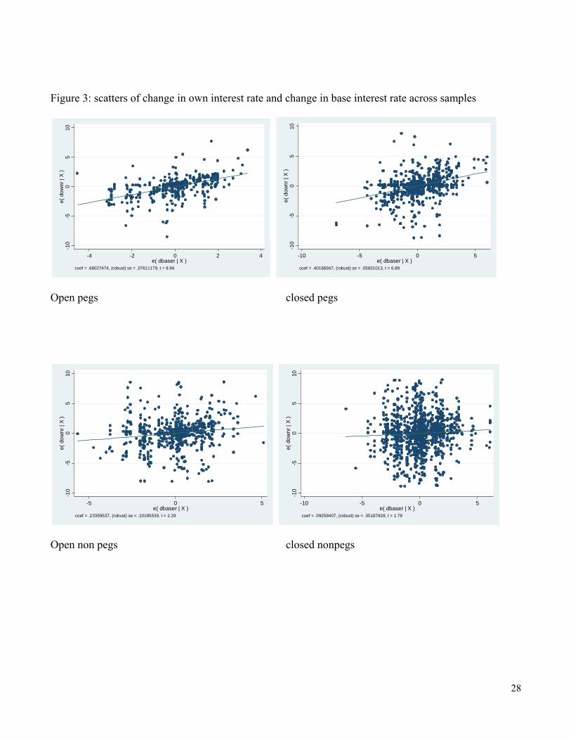
28  

Figure 3: scatters of change in own interest rate and change in base interest rate across samples

Open pegs closed pegs

 

 

   

Open non pegs closed nonpegs

-10

-50

510

e( d

ow

nr

| X )

-4 -2 0 2 4e( dbaser | X )

coef = .68027474, (robust) se = .07611179, t = 8.94

-10

-50

510

e( d

ow

nr

| X )

-10 -5 0 5e( dbaser | X )

coef = .40166567, (robust) se = .05831013, t = 6.89

-10

-50

510

e( d

ow

nr

| X )

-5 0 5e( dbaser | X )

coef = .23359537, (robust) se = .10195539, t = 2.29

-10

-50

510

e( d

ow

nr

| X )

-10 -5 0 5e( dbaser | X )

coef = .09259407, (robust) se = .05187828, t = 1.78

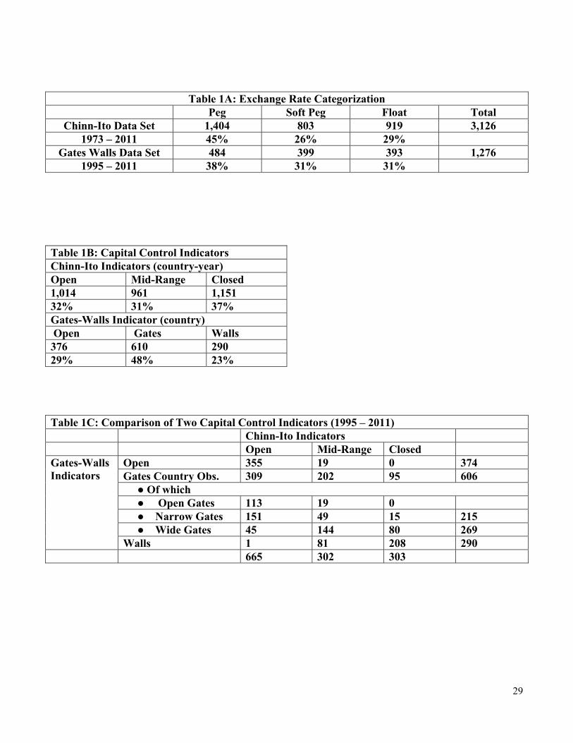
29  

Table 1A: Exchange Rate Categorization Peg Soft Peg Float Total

Chinn-Ito Data Set 1,404 803 919 3,126 1973 – 2011 45% 26% 29%

Gates Walls Data Set 484 399 393 1,276 1995 – 2011 38% 31% 31%

Table 1B: Capital Control Indicators Chinn-Ito Indicators (country-year) Open Mid-Range Closed 1,014 961 1,151 32% 31% 37% Gates-Walls Indicator (country) Open Gates Walls 376 610 290 29% 48% 23%

Table 1C: Comparison of Two Capital Control Indicators (1995 – 2011) Chinn-Ito Indicators Open Mid-Range Closed Gates-Walls Indicators

Open 355 19 0 374 Gates Country Obs. 309 202 95 606 ● Of which ● Open Gates 113 19 0 ● Narrow Gates 151 49 15 215 ● Wide Gates 45 144 80 269 Walls 1 81 208 290

665 302 303

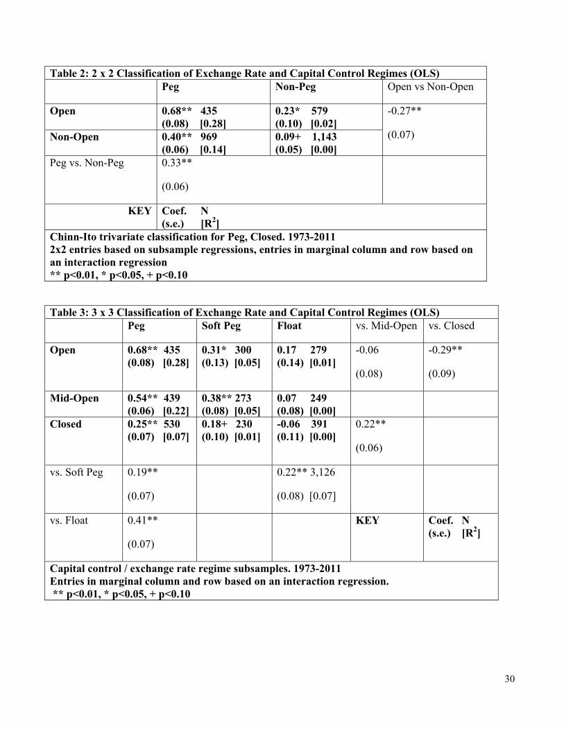
30  

Table 2: 2 x 2 Classification of Exchange Rate and Capital Control Regimes (OLS) Peg Non-Peg Open vs Non-Open

Open 0.68** 435 (0.08) [0.28]

0.23* 579 (0.10) [0.02]

-0.27**

(0.07) Non-Open 0.40** 969 (0.06) [0.14]

0.09+ 1,143 (0.05) [0.00]

Peg vs. Non-Peg 0.33**

(0.06)

KEY Coef. N (s.e.) [R2]

Chinn-Ito trivariate classification for Peg, Closed. 1973-2011 2x2 entries based on subsample regressions, entries in marginal column and row based on an interaction regression ** p<0.01, * p<0.05, + p<0.10

Table 3: 3 x 3 Classification of Exchange Rate and Capital Control Regimes (OLS) Peg Soft Peg Float vs. Mid-Open vs. Closed

Open 0.68** 435 (0.08) [0.28]

0.31* 300 (0.13) [0.05]

0.17 279 (0.14) [0.01]

-0.06

(0.08)

-0.29**

(0.09)

Mid-Open 0.54** 439 (0.06) [0.22]

0.38** 273 (0.08) [0.05]

0.07 249 (0.08) [0.00]

Closed 0.25** 530 (0.07) [0.07]

0.18+ 230 (0.10) [0.01]

-0.06 391 (0.11) [0.00]

0.22**

(0.06)

vs. Soft Peg 0.19**

(0.07)

0.22** 3,126

(0.08) [0.07]

vs. Float 0.41**

(0.07)

KEY Coef. N (s.e.) [R2]

Capital control / exchange rate regime subsamples. 1973-2011 Entries in marginal column and row based on an interaction regression. ** p<0.01, * p<0.05, + p<0.10

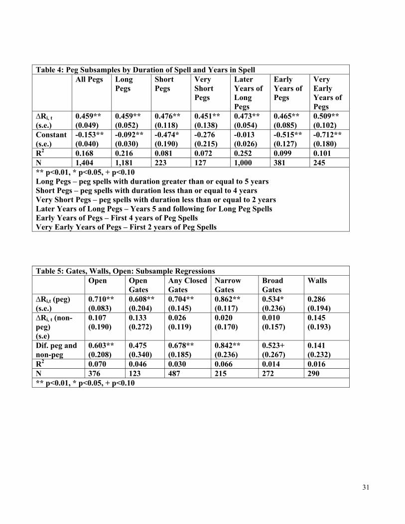
31  

Table 4: Peg Subsamples by Duration of Spell and Years in Spell All Pegs Long

Pegs Short Pegs

Very Short Pegs

Later Years of Long Pegs

Early Years of Pegs

Very Early Years of Pegs

∆Ri, t

(s.e.) 0.459** (0.049)

0.459** (0.052)

0.476** (0.118)

0.451** (0.138)

0.473** (0.054)

0.465** (0.085)

0.509** (0.102)

Constant (s.e.)

-0.153** (0.040)

-0.092** (0.030)

-0.474* (0.190)

-0.276 (0.215)

-0.013 (0.026)

-0.515** (0.127)

-0.712** (0.180)

R2 0.168 0.216 0.081 0.072 0.252 0.099 0.101 N 1,404 1,181 223 127 1,000 381 245 ** p<0.01, * p<0.05, + p<0.10 Long Pegs – peg spells with duration greater than or equal to 5 years Short Pegs – peg spells with duration less than or equal to 4 years Very Short Pegs – peg spells with duration less than or equal to 2 years Later Years of Long Pegs – Years 5 and following for Long Peg Spells Early Years of Pegs – First 4 years of Peg Spells Very Early Years of Pegs – First 2 years of Peg Spells

Table 5: Gates, Walls, Open: Subsample Regressions Open Open

Gates Any Closed Gates

Narrow Gates

Broad Gates

Walls

∆Ri,t (peg) (s.e.)

0.710** (0.083)

0.608** (0.204)

0.704** (0.145)

0.862** (0.117)

0.534* (0.236)

0.286 (0.194)

∆Ri, t (non-peg) (s.e)

0.107 (0.190)

0.133 (0.272)

0.026 (0.119)

0.020 (0.170)

0.010 (0.157)

0.145 (0.193)

Dif. peg and non-peg

0.603** (0.208)

0.475 (0.340)

0.678** (0.185)

0.842** (0.236)

0.523+ (0.267)

0.141 (0.232)

R2 0.070 0.046 0.030 0.066 0.014 0.016 N 376 123 487 215 272 290 ** p<0.01, * p<0.05, + p<0.10

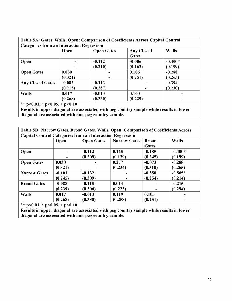
32  

Table 5A: Gates, Walls, Open: Comparison of Coefficients Across Capital Control Categories from an Interaction Regression Open Open Gates Any Closed

Gates Walls

Open - -

-0.112 (0.210)

-0.006 (0.162)

-0.400* (0.199)

Open Gates 0.030 (0.321)

- -

0.106 (0.251)

-0.288 (0.265)

Any Closed Gates -0.082 (0.215)

-0.113 (0.287)

- -

-0.394+ (0.230)

Walls 0.017 (0.268)

-0.013 (0.330)

0.100 (0.229)

- -

** p<0.01, * p<0.05, + p<0.10 Results in upper diagonal are associated with peg country sample while results in lower diagonal are associated with non-peg country sample.

Table 5B: Narrow Gates, Broad Gates, Walls, Open: Comparison of Coefficients Across Capital Control Categories from an Interaction Regression Open Open Gates Narrow Gates Broad

Gates Walls

Open - -

-0.112 (0.209)

0.165 (0.139)

-0.185 (0.245)

-0.400* (0.199)

Open Gates 0.030 (0.321)

- -

0.277 (0.234)

-0.073 (0.310)

-0.288 (0.265)

Narrow Gates -0.103 (0.245)

-0.132 (0.309)

- -

-0.350 (0.254)

-0.565* (0.214)

Broad Gates

-0.088 (0.239)

-0.118 (0.306)

0.014 (0.223)

- -

-0.215 (0.294)

Walls 0.017 (0.268)

-0.013 (0.330)

0.119 (0.258)

0.105 (0.251)

- -

** p<0.01, * p<0.05, + p<0.10 Results in upper diagonal are associated with peg country sample while results in lower diagonal are associated with non-peg country sample.

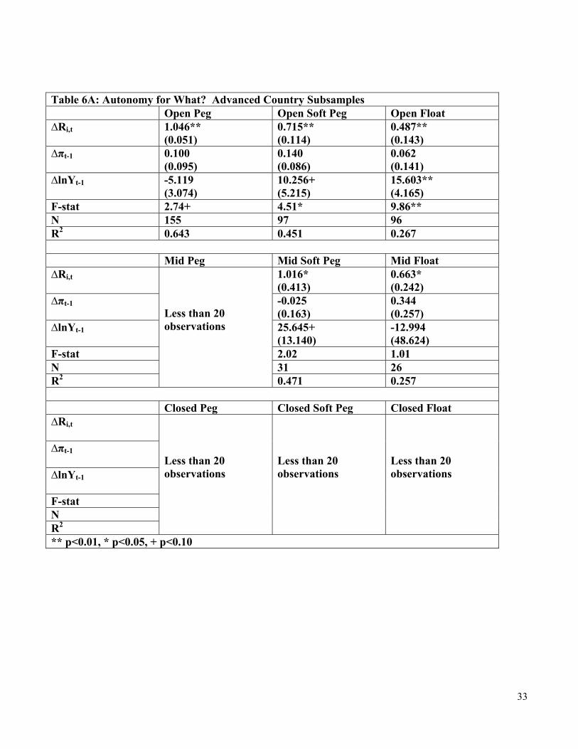
33  

Table 6A: Autonomy for What? Advanced Country Subsamples Open Peg Open Soft Peg Open Float ∆Ri,t

1.046** (0.051)

0.715** (0.114)

0.487** (0.143)

∆πt-1

0.100 (0.095)

0.140 (0.086)

0.062 (0.141)

∆lnYt-1

-5.119 (3.074)

10.256+ (5.215)

15.603** (4.165)

F-stat 2.74+ 4.51* 9.86** N 155 97 96 R2 0.643 0.451 0.267 Mid Peg Mid Soft Peg Mid Float ∆Ri,t

Less than 20 observations

1.016* (0.413)

0.663* (0.242)

∆πt-1

-0.025 (0.163)

0.344 (0.257)

∆lnYt-1

25.645+ (13.140)

-12.994 (48.624)

F-stat 2.02 1.01 N 31 26 R2 0.471 0.257 Closed Peg Closed Soft Peg Closed Float ∆Ri,t

Less than 20 observations

Less than 20 observations

Less than 20 observations

∆πt-1 ∆lnYt-1 F-stat N R2 ** p<0.01, * p<0.05, + p<0.10

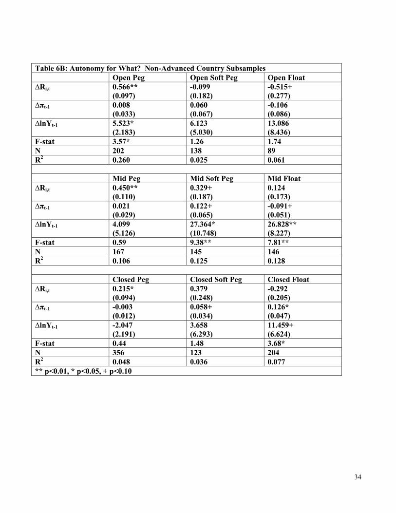
34  

Table 6B: Autonomy for What? Non-Advanced Country Subsamples Open Peg Open Soft Peg Open Float ∆Ri,t

0.566** (0.097)

-0.099 (0.182)

-0.515+ (0.277)

∆πt-1

0.008 (0.033)

0.060 (0.067)

-0.106 (0.086)

∆lnYt-1

5.523* (2.183)

6.123 (5.030)

13.086 (8.436)

F-stat 3.57* 1.26 1.74 N 202 138 89 R2 0.260 0.025 0.061 Mid Peg Mid Soft Peg Mid Float ∆Ri,t

0.450** (0.110)

0.329+ (0.187)

0.124 (0.173)

∆πt-1

0.021 (0.029)

0.122+ (0.065)

-0.091+ (0.051)

∆lnYt-1

4.099 (5.126)

27.364* (10.748)

26.828** (8.227)

F-stat 0.59 9.38** 7.81** N 167 145 146 R2 0.106 0.125 0.128 Closed Peg Closed Soft Peg Closed Float ∆Ri,t

0.215* (0.094)

0.379 (0.248)

-0.292 (0.205)

∆πt-1

-0.003 (0.012)

0.058+ (0.034)

0.126* (0.047)

∆lnYt-1

-2.047 (2.191)

3.658 (6.293)

11.459+ (6.624)

F-stat 0.44 1.48 3.68* N 356 123 204 R2 0.048 0.036 0.077 ** p<0.01, * p<0.05, + p<0.10

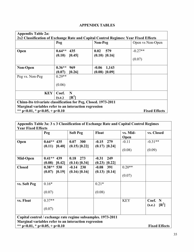
35  

APPENDIX TABLES

Appendix Table 2a: 2x2 Classification of Exchange Rate and Capital Control Regimes: Year Fixed Effects Peg Non-Peg Open vs Non-Open

Open 0.64** 435 (0.10) [0.45]

0.02 579 (0.10) [0.16]

-0.27**

(0.07)

Non-Open 0.36** 969 (0.07) [0.26]

-0.06 1,143 (0.08) [0.09]

Peg vs. Non-Peg 0.29**

(0.06)

KEY Coef. N (s.e.) [R2]

Chinn-Ito trivariate classification for Peg, Closed. 1973-2011 Marginal variables refer to an interaction regression ** p<0.01, * p<0.05, + p<0.10 Fixed Effects

Appendix Table 3a: 3 x 3 Classification of Exchange Rate and Capital Control Regimes Year Fixed Effects Peg Soft Peg Float vs. Mid-

Open vs. Closed

Open 0.64** 435 (0.11) [0.40]

0.07 300 (0.15) [0.22]

-0.15 279 (0.17) [0.24]

-0.11

(0.08)

-0.31**

(0.09)

Mid-Open 0.41** 439 (0.08) [0.42]

0.18 273 (0.14) [0.34]

-0.31 249 (0.23) [0.22]

Closed 0.38** 530 (0.07) [0.19]

-0.14 230 (0.16) [0.16]

-0.08 391 (0.13) [0.14]

0.20**

(0.07)

vs. Soft Peg 0.16*

(0.07)

0.21*

(0.08)

vs. Float 0.37**

(0.07)

KEY Coef. N (s.e.) [R2]

Capital control / exchange rate regime subsamples. 1973-2011 Marginal variables refer to an interaction regression ** p<0.01, * p<0.05, + p<0.10 Fixed Effects

36