Embed Size (px)
Citation preview

Monetary policy and exchange rate overshooting: Dornbusch was right after all
Hilde C. Bjørnland* University of Oslo and Norges Bank
First draft: November 2005 This draft: June 2006
Abstract Dornbusch’s exchange rate overshooting hypothesis is a central building block in international macroeconomics. Yet, empirical studies of monetary policy have typically found exchange rate effects that are inconsistent with overshooting. This puzzling result has by some researches been viewed as a “styled facts” to be reckoned with in policy modelling. However, many of these studies, in particular those using VARs, have disregarded the strong contemporaneous interaction between monetary policy and exchange rate movements by placing zero restriction on them. In contrast, I achieve identification by imposing a long-run neutrality restriction on the real exchange rate, thereby allowing for contemporaneous interaction between the interest rate and the exchange rate. In a study of five open economies, I find that the puzzles disappear. In particular, a contractionary monetary policy shock has a strong effect on the exchange rate that appreciates on impact. The maximum effect occurs immediately, and the exchange rate thereafter gradually depreciates to baseline, consistent with the Dornbusch overshooting hypothesis and with few exceptions consistent with UIP.
Keywords: Exchange rate; uncovered interest parity (UIP); Dornbusch overshooting; monetary policy; Structural VAR. JEL-codes: C32, E52, F31, F41
* Department of Economics, University of Oslo. E-mail: [email protected]. This paper has previously been circulated under the title: “Monetary Policy and the Illusionary Exchange Rate Puzzle”. Detailed comments from Steinar Holden are gratefully acknowledged. I have also benefited from discussions with Leif Brubakk, Carlo A. Favero, Nils Gottfries, Kai Leitemo, Jesper Lindé, Sharon McCaw, Kjetil Olsen, Asbjørn Rødseth, Luca Sala, and participants at seminars at Sveriges Riksbank, Uppsala University, Norges Bank and at the CEF06 conference in Cypros and the University of Oslo workshop on “Model evaluation in macroeconomics”. Thanks to Kathrine Lund for collecting the data. The views expressed in this paper are those of the author and should not be interpreted as reflecting the views of Norges Bank.
1 Introduction Dornbusch’s (1976) well known exchange rate overshooting hypothesis is a central building block in international macroeconomics; stating that an increase in the interest rate should cause the nominal exchange rate to appreciate instantaneously, for then to depreciate in line with uncovered interest parity (UIP). Its influence is evident in the rapidly growing “New Open Economy Macroeconomics” (NOEM) literature (see Obstfeld and Rogoff, 1995, 2000) as well as in practical policy discussions spanning far outside the academic sphere. With what seems like an ever-increasing number of citations, it has been described as one of the most important papers in international economics over the entire twentieth century (Rogoff, 2002).
When confronted with data, however, few empirical studies analysing the effects of monetary policy have found support for Dornbusch overshooting, see e.g. Sims (1992), Eichenbaum and Evans (1995) and Kim and Roubini (2000) for G7 countries, Peersman and Smets (2003) and Favero and Marcellino (2004) for the aggregate Euro area, Mojon and Peersman (2003) for individual Euro area countries and Lindé (2003) for Sweden. Instead, they have found that following a contractionary monetary policy shock, the real exchange rate either depreciates, or, if it appreciates, it does so only gradually and for a prolonged period of up to three years, thereby giving a hump-shaped response that violates UIP. In the literature, the first phenomenon has been termed the exchange rate puzzle, whereas the second has been referred to as delayed overshooting or forward discount puzzle, see Cushman and Zha (1997).1 In light of all this evidence that is inconsistent with Dornbusch overshooting and UIP, one might perhaps expect the theory to be abandoned by economists. Yet, this is not the case, both the hypothesis of Dornbusch overshooting and the UIP remain at the core in theories of international economics. The elegance and clarity of the Dornbusch model as well as its obvious policy relevance has put it in a separate class from other international macroeconomic papers (Rogoff, 2002).
The common approach for establishing the quantitative effects of monetary policy in the above mentioned studies has been the structural vector autoregressive (VAR) approach, which was first initiated by Sims (1980).2 There is, however, a major challenge when analyzing the open economy through structural VARs; namely how to properly address the simultaneity problem between monetary policy and the exchange rate. Most of the VAR studies of open economies (including those mentioned above), deal with a possible simultaneity problem by placing recursive, zero contemporaneous restrictions on the interaction between monetary policy and exchange rates.3 However, by not allowing for potential simultaneity effects in the identification of monetary policy shock, they may have produced a numerically important bias in the estimate of the degree of interdependence.
1 The finding that UIP does not hold is not new; see Fama (1984) for a contribution to the international finance literature and Engel (1996) for survey. However, the VAR literature focuses on whether UIP holds conditionally with respect to monetary policy. 2 For the role of VAR models in policy analysis, see for instance Greenspan (2005). 3 To be precise, Kim and Roubini (2000) allow for a contemporaneous interaction between monetary policy and the exchange rate, but assume instead that the monetary policymaker do not respond contemporaneously to changes in the foreign interest rate. As a result they observe fewer puzzles in the exchange rates than other studies, although for some countries (notably Canada and Germany), a pronounced delay overshooting puzzle still remains.
2
This point has recently been emphasized by Faust and Rogers (2003). By dropping one after one of what they call dubious restrictions, they find that the responses in the exchange rate to (U.S.) monetary policy are sensitive to the zero short-run restrictions imposed (whether it is between the interest rate and exchange rate responses as assumed in the majority of VARs, or between the domestic and foreign interest rate as assumed in Kim and Roubini, 2000). Their results allow for an early peak in the exchange rate, which might give a role for the conventional overshooting model. However, the effect is not uniquely identified, so no robust conclusions can be drawn with regard to the exact timing of the peak response - which could be immediate or delayed. Furthermore, even if they could justify an early peak, they find that the identified monetary policy shocks can not generate interest rate and exchange rate responses consistent with UIP. The bulk of the variance of the exchange rate is instead due to other non-monetary shocks.4 Hence, the implied interest rate and exchange rate responses following a monetary policy shock continue to remain distinct from Dornbusch's prediction, with both the delayed overshooting feature and/or deviation from UIP emerging as consensus. In fact, some researchers now view the puzzles themselves as stylized facts, which recently developed “Dynamic Stochastic General Equilibrium” (DSGE) models should seek to replicate, see e.g. Smets and Wouters (2002), Lindé et al. (2004), Murchison et al. (2004) and Adolfson et al. (2006). However, as DSGE models have begun to dominate the field of applied macroeconomics and policymaking, it seems now more likely that the economic profession might eventually abandon the Dornbusch overshooting model – also in theory. This paper strongly cautions against allowing for exchange rate puzzles to develop into consensus for the following reason. Although the approach of Faust and Roger (2003) in testing dubious restrictions does not require full identification, drawing inference with regard to the precise timing of peak response in the exchange rate clearly does. This suggests that one should seek to identify VAR models by applying restrictions that allow for a unique identification while maintaining the contemporaneous interaction between monetary policy and the exchange rate intact. Doing exactly so, I find that the Dornbusch overshooting results hold after all. To be more precise, in this paper I suggest identification by restricting the long run multipliers of shocks. In particular, I assume that monetary policy shocks can have no long run effect on the level of the real exchange rate. In the short run, however, monetary policy is free to influence the exchange rate. Eventually though, the effect dies out and the real exchange rate returns to its initial level. This is a standard neutrality assumption that holds for a large class of models in the monetary policy literature (see Obstfeld, 1985; Clarida and Gali, 1994).
Once allowing for a contemporaneous relationship between the interest rate and the exchange rate, the remaining VAR can be identified using standard recursive zero restrictions on the impact matrix of shocks; assuming a lagged response in domestic variables (such as
4 Similar results are also found in Scholl and Uhlig (2005), using a related procedure to that of Faust and Rogers (2003). However, they also find that the exchange rate might depreciate on impact following a contractionary monetary policy shock (exchange rate puzzle).
3
output and inflation) to monetary policy shocks. These restrictions are less controversial and studies identifying monetary policy without these restrictions have found qualitatively similar results, see for example Faust et al. (2004) and the references therein. Furthermore, the assumption of a delayed response in output and inflation combined with a long run neutrality restriction on the real exchange rate following a monetary policy surprise, are core assumptions underlying the Dornbusch’s overshooting model; consistent with NOEM implications (Lane, 2001) and are empirically realistic (Rogoff, 2002).
I use the alternative identification strategy on five small open economies with floating exchange rates; Australia, Canada, New Zealand, Sweden and the UK, and the results are striking.5 Contrary to the findings of recent studies, I find that a contractionary monetary policy shock has a strong effect on the exchange rate that appreciates on impact. The maximal impact occurs immediately, and the exchange rate thereafter gradually depreciates back to baseline; consistent with the Dornbusch overshooting hypothesis and with few exceptions consistent with UIP.
Small open countries are chosen to analyse the effect of Dornbusch overshooting, as the exchange rate is an important transmission channel for shocks in open economies. Furthermore, these countries have all adopted an inflation targeting framework for monetary policy, in which the perceived effect of the exchange rate for inflation is of crucial importance in the monetary policy decision making (Taylor, 2001). In fact, the empirical analysis also confirms that there is a systematic interest rate response to exchange rate movements in all countries, making the identification of the interdependence between monetary policy and exchange rate movements a non-trivial issue.
An alternative (non-VAR) approach to studying the impact of monetary policy shocks on the exchange rate is through event studies. Event studies ensure identification by measuring the immediate response of the exchange rate to shocks associated with particular policy actions in real time. In sharp contrast to the majority of VAR studies, recent event studies have found that a surprise contractionary monetary policy shock has a substantial appreciating effect on the exchange rate, see for instance Bonser-Neal et al. (1998), Zettelmeyer (2004) and Kearns and Manners (2005). This link between surprise monetary policy actions and initial exchange rate responses is therefore a feature that properly identified VAR models should be able to replicate. However, event studies, with their exclusive focus on the immediate response, cannot answer questions about the speed of overshooting. To do so, one needs to identify monetary policy shocks in a system like the structural VARs, as is done in the present study. However, I find it comforting that my results are consistent with the evidence from the event studies.
The paper is organised as follows. Section 2 discusses the VAR methodology used to identify monetary policy shocks and section 3 presents the empirical results. Section 4 provides robustness checks and Section 5 concludes.
5 See also Bjørnland (2005) for a more detailed analysis of Norway that finds corroborate results.
4
2 The structural VAR model The variables in the VAR model are chosen to reflect the theoretical set up of a New-Keynesian small open economy model, such as that described in Clarida et al. (2001) and Svensson (2000). In particular, the VAR model comprises log of real GDP (yt), log of the quarterly changes in the consumer price index (CPI) (πt) – referred to hereafter as inflation, the three month domestic interest rate (it), the trade-weighted foreign interest rate (it*) and the log of the real trade-weighted exchange rate (et) (see appendix A for details). I follow the traditional closed economy VAR literature (Blanchard, 1989, Christiano et al., 1999, 2005, among many others), in that a standard recursive structure is identified between macroeconomic variables and monetary policy, so that macroeconomic variables such as output and inflation do not react contemporaneously to monetary shocks, whereas there might be a simultaneous feedback from the macro environment to monetary variables. That monetary policy affects domestic variables with a lag, is consistent with the transmission mechanism of monetary policy emphasised in the theoretical set up in Svensson (1997). Further, Bagliano and Favero (1998) show that when monetary policy shocks are identified in this recursive way on a single monetary policy regime, the responses of the shocks suggest a pattern for the monetary transmission mechanism that is consistent with the impulse responses of monetary policy shocks identified instead using financial market information from outside the VAR, as in Rudebusch (1998). With regard to the open economy applications, most studies have identified monetary policy shocks by using a Cholesky decomposition that either i) restricts the (systematic) monetary policy from reacting contemporaneously to an exchange rate shock, or ii) restricts the exchange rate from reacting immediately to a monetary policy shock. The first restriction (see e.g. Sims, 1992; Eichenbaum and Evans, 1995 for initial applications), is equivalent to assuming that the monetary authority ignores any surprise movement in exchange rates that have occurred during the time in which decisions on the policy variables are made. For small open economies, this seems far from practical monetary policy settings. The exchange rate is an important transmission channel for foreign shocks that the central bank may respond to within the month or quarter, which is the usual sampling frequency in these studies. Furthermore, the exchange rate, being an asset price, is inherently a forward-looking and expectations-determined variable that will reflect expected future return on the asset. This may by itself provide important information about the expected development of the determinants of the targeting variables that the central bank may want react to, see Obstfeld and Rogoff (1995) and Taylor (2001) for arguments, and Clarida et al. (1998) for empirical evidence. The second set of restrictions commonly used, namely that the exchange rate can not react immediately to a monetary policy shock (i.e. Favero and Marcellino, 2004; Mojon and Peersman, 2003, among others), is also hard to square with basic economic theory. The exchange rate is an asset price that will reflect expected future return on the asset. As news on monetary policy will change the expected return on assets, the exchange rate should react instantaneously to monetary policy. This has been confirmed recently in a series of event studies; see e.g. Zettelmeyer (2004) among others. Finally, delay reactions in the exchange
5
rate seem inconsistent with the observed volatile behaviour of exchange rates in the post Bretton Woods era. Hence, both of these restrictions are inconsistent with established theory and also in contrast to how practitioners view the relationship between the interest rate and the exchange rate in small open economies. The structural shocks should therefore not be recovered using either of these recursive restrictions on the parameters. It is, however, fair to say that several of the authors using traditional VARs have been concerned about the validity of these restrictions and have investigated their implications by rearranging the direction of causation between the interest rate and the exchange rate to see if that makes a difference. However, it is not clear if this strategy will produce the correct impulse responses if there is a genuine simultaneous relationship between the two variables. This will effectively be demonstrated below. The present approach differs from the more traditional methods in that I allow for full simultaneity between monetary policy and exchange rate responses. Instead I assume that monetary policy shocks are restricted from having long-run effects on real exchange rates. As already emphasised, this is a standard neutrality assumption that holds for a large class of models in the monetary policy literature.6 In particular, Clarida and Gali (1994) show that this kind of restriction on the real exchange rate is consistent with a stochastic version of the two country, rational expectations open-macro model developed by Obstfeld (1985). The model exhibits the standard Mundell-Fleming-Dornbusch results in the short run when prices reacts sluggishly, but in the long run, prices adjust fully to all shocks. 2.1 Identification In the following I define Zt as the (5x1) vector of the macroeconomic variables discussed
above, *, , , ,t t t t t t 'Z i y i eπ⎡= ⎣ ⎤∆ ⎦
t
, where all variables but the real exchange rate are for now
assumed to be stationary7. Zt can be written in terms of its moving average (ignoring any deterministic terms)
( )tZ B L ν= , (1)
where vt is a (5x1) vector of reduced form residuals assumed to be identically and independently distributed, vt ~ iid(0,Ω), with positive definite covariance matrix Ω. B(L) is the
(5x5) convergent matrix polynomial in the lag operator L, 0
( ) jjj
B L B∞
== L∑ . Following the
literature, the underlying orthogonal structural disturbances (εt) are assumed to be written as
linear combinations of the innovations (vt), i.e., tv S tε= . The VAR can then be written in
terms of the structural shocks as
6 Bjørnland and Leitemo (2004) explore, in a similar vein, the use of short and long run restrictions in order to identify the interdependence of stock prices and monetary policy in a structural VAR of a closed economy. 7 This assumption is further discussed in the empirical analysis below.
6
( )t tZ C L ε= , (2)
where ( ) ( )B L S C L= . Clearly, if S is identified, one can derive the MA representation in (2)
since B(L) can be calculated from a reduced form estimation. Hence, to go from the reduced form VAR to the structural interpretation, one needs to apply restrictions on the S matrix. Only then can one recover the relevant structural parameters from the covariance matrix of the reduced form residuals.
To identify S, the εt‘s are assumed to be normalised so they all have unit variance.
The normalisation of cov(εt) implies that SS’ = Ω. With a five variable system, this imposes 15 restrictions on the elements in S. However, as the S matrix contains 25 elements, to orthogonalise the different innovations, ten more restrictions are needed.
With a five variables VAR, one can identify five structural shocks. The first two are of primary interest and are interpreted as monetary policy shocks (εt
MP) and real exchange rate shocks (εt
ER). I follow standard practice in the VAR literature and only loosely identify the last three shocks as inflation shocks (interpreted as cost push shocks) (εt
CP), output shocks (εt
Y) and foreign interest rate shocks (εti*). Ordering the vector of structural shocks as
and following the standard closed economy literature in
identifying monetary policy shocks, the recursive order between monetary policy shocks and the (domestic) macroeconomic variables implies the following restriction on the S matrix
*, , , ,i Y CP MP ERt t t t t tε ε ε ε εε⎡= ⎣ '⎤⎦
ε
*
11
21 22
31 32 33
41 42 43 44 45
51 52 53 54 55
0 0 0 0* 0 0 0
( ) 0 0
i
Y
CP
MP
ERt t
SiS Sy
B L S S Si S S S S S
e S S S S S
εε
π
ε
ε
⎡ ⎤⎡ ⎤⎡ ⎤ ⎢ ⎥⎢ ⎥⎢ ⎥ ⎢ ⎥⎢ ⎥⎢ ⎥ ⎢ ⎥⎢ ⎥⎢ ⎥ = ⎢ ⎥⎢ ⎥⎢ ⎥ ⎢ ⎥⎢ ⎥⎢ ⎥ ⎢ ⎥⎢ ⎥⎢ ⎥∆⎣ ⎦ ⎣ ⎦ ⎢ ⎥⎣ ⎦
. (3)
The foreign interest rate is placed on the top of the ordering, assuming it will only be affected by exogenous foreign monetary policy contemporaneously; a plausible small country assumption. Furthermore, the recursive restriction commonly used in the closed economy literature (namely that domestic variables such as output and inflation react with a lag to the policy variables, while there is a simultaneous reaction from the economic environment to policy variables), is taken care of by placing the domestic variables above the interest rate in the ordering, and assuming zero restrictions on the relevant coefficients in the S matrix as shown in (3). However, by examining the relevant columns in S, one can interpret the domestic shocks somewhat further. In particular, while price shocks can affect all variables but output contemporaneously, output shocks can affect both output and prices contemporaneously. Hence, it seems reasonable to interpret a price shock as a cost push shock (moving prices before output), whereas output shocks will be dominated by both demand
7
shocks and supply shocks.8 This provides nine contemporaneous restrictions directly on the S matrix.
The matrix is still one restriction short of identification. The standard practice in the VAR literature, namely to place the exchange rate last in the ordering and assuming S45 = 0, so that monetary variables are restricted from reacting simultaneously to the exchange rate shock, while the exchange rate is allowed to react simultaneously to all shocks, would have provided enough restriction to identify the system, thereby allowing for the use of the standard Cholesky recursive decomposition.
However, if that restriction is not valid but is nonetheless imposed, the estimated responses to the structural shocks will be severely biased. Instead, the restriction that a monetary policy shock can have no long-run effects on the real exchange rate is imposed, which as discussed above, is a plausible neutrality assumption. This can be found by setting
the values of the infinite number of relevant lag coefficients in (2), 54,0 jjC∞
=∑ , equal to zero.
By using this long-run restriction, there are enough restrictions to identify and orthogonalise all shocks. Writing the long-run expression of ( ) ( )B L S C L= as
(1) (1)B S C= , (4)
where 0
(1) jjB B∞
== ∑ and
0(1) jj
C ∞
== C∑ indicate the (5x5) long-run matrix of B(L) and
C(L) respectively, the long-run restriction that C54(1) = 0 implies
. (5) 51 14 52 24 53 34 54 44 55 54(1) (1) (1) (1) (1) 0B S B S B S B S B S+ + + + =
Hence, by replacing one contemporaneous restriction with a long run neutrality restriction, the model is now uniquely identified. The restrictions allows for contemporaneous interaction between monetary policy and exchange rate dynamics, without having to resort to methods that deviate extensively from the established view of how one identify monetary policy shocks in the closed economy literature. Furthermore, the long run neutrality assumption used is theoretically appealing, being consistent with the underlying assumptions in the Dornbusch’s overshooting model. Yet, introducing a new restriction does not come without any type of costs. In particular, using an infinite (long run) restriction on finite dimension VAR may provide unreliable estimates, unless the economy satisfies some types of strong restrictions on the finite horizon (see Faust and Leeper, 1997). Although potentially a problem, I argue that the joint use of short run and long run constraints used in the present VAR model, should be sufficient to side-step some of this criticism.9
8 I have also experienced with alternating the order of the first three variables in Z, without much effects on results. 9 Strictly speaking, Faust and Leeper’s (1997) critique refers to a bivariate model like Blanchard and Quah (1989) that use one long run restriction. Their problem stems from the fact that the underlying model has more sources of shocks (with sufficiently different dynamic effects on the variables considered) than does the estimated model.
8
3 Empirical results The model is estimated for Australia, Canada, New Zealand, Sweden and UK. Quarterly data from 1983Q1 to 2004Q4 are used, except for New Zealand. Using an earlier starting period than 1983 will make it hard to identify a stable monetary policy regime, as monetary policy prior to 1983 has experienced important structural changes and unusual operating procedures that would imply severe parameter instability (see for instance Bagliano and Favero, 1998; Clarida et al., 2000). For New Zealand, the start date is set to 1988 as the period 1983-1987 is characterised with a high degree of volatility when New Zealand changed from a closed and centrally controlled economy to one of the most open countries in the OECD (see Evans et al., 1996). Below, robustness checks are nevertheless performed for all countries by extending the sample backwards and forwards in time. There are no qualitative changes to the results. Consistent with most other related studies, the variables, with the exception of the real exchange rate, are specified in levels.10 This implies that any potential cointegrating relationship between non-stationary variables will be implicitly determined in the model (see Hamilton, 1994).11 Sims, Stock and Watson (1990) also argue for using VAR in levels as a modelling strategy, as one avoids the danger of inconsistency in the parameters caused by imposing incorrect cointegrating restrictions; though at the cost of reducing efficiency. One may argue (Giordani, 2004) that with the theoretical model of Svensson (1997) as a data generating process, rather than including output in levels, one should either include the output gap in the VAR, or the output gap along with the trend level of output. However, as pointed out by Lindé (2003), a practical point that Giordani does not address is how to compute trend output (thereby also the output gap). I therefore instead follow Lindé (2003) and include a linear trend in the VAR along with output in levels. In that way I try to address this problem by modelling the trend implicit in the VAR.
The real exchange rate is clearly non-stationary and is differenced to obtain stationarity. By applying long-run restrictions to the first-differenced real exchange rate, the effects of monetary policy shocks on the level of the exchange rate will eventually sum to zero (c.f. Blanchard and Quah 1989).12
The lag order of the VAR-model is determined using the Schwarz and Hannan-Quinn information criteria and the F-forms of likelihood ratio tests for model reductions. Most tests suggested that three lags were acceptable for all countries, although some indicate four lags. With a relatively short sample, I therefore decided to use three lags in the estimation and check for robustness using alternative lag lengths. With three lags, the hypothesis of autocorrelation and heteroscedasticty is rejected for all countries, although some non-normality remained in the system. In a few cases impulse dummies (that take the value 1 in
10 Based on the standard Augmented Dickey Fuller (ADF) unit root test, I can not reject that any of the variables except possibly inflation are integrated of first order. However, due to the low power of the ADF tests to differentiate between a unit root and a (trend-) stationary process, I can not rule out that most of the variables could equally well be represented in levels 11 There is little evidence of any cointegration relationship at the outset, with the hypothesis of one cointegration vector being at most accepted. 12 Various tests suggest that I can not reject the hypothesis of a unit root in the real exchange rate, indicating that it is non-stationary. The ADF t-statistics are tADF =-1.806, tADF =-0.5625, tADF =-2.381, tADF =-2.631 and tADF =-2.543 for Australia, Canada, New Zealand, Sweden and the UK respectively (two lags). Using alternative lag lengths or extending the sample backwards to 1973/78 yield similar results.
9
one quarter and 0 otherwise) were included, to take account of extreme outliers. That is, for Sweden, three dummies were included; 1992Q3, 1993Q1 and 1995Q4, where the first captures an exceptionally high interest rate increase (almost 500 percent) implemented by the Riksbank in order to defend the Swedish exchange rate (see also the discussion in Lindé 2003), the second reflects the subsequent floating of the Swedish krona and the final one captures additional turbulence in the exchange rate. For Australia two dummies were included; 1984Q1 and 2000Q3, that reflected a substantial decrease and increase in the inflation rate respectively. With these dummies incorporated, some non-normality nevertheless remained, although mainly in the foreign interest rate equation. However, the Chow break tests suggested that all countries had stable equations; hence I decided to ignore any remaining non-normality.13 3.1 Cholesky decomposition For comparison, I start by briefly discussing the results using a standard Cholesky ordering, before turning to the preferred structural decomposition in section 3.2 below. The purpose of this exercise is to show that by using very similar identification schemes to what has been standard practice in the literature, I obtain the same pattern of delayed overshooting that has been found in the many previous VAR studies discussed above. Figure 1 shows the impulse responses for the interest rate and the exchange rate from a monetary policy shock, using two different Cholesky orderings. The solid line corresponds to the baseline Cholesky assumption that an exchange rate shock has no immediate effect on the interest rate, whereas the dotted line corresponds to an ordering where monetary policy shock has no immediate effect on the real exchange rate. In the figures below, the effect of the monetary policy shock is normalised so that the interest rate increases by one percentage point the first quarter. Note that a decrease in the real exchange rate implies appreciation.14
Focusing first on the baseline Cholesky ordering (solid line), we see that no country exhibits an exchange rate response in line with Dornbusch overshooting. In Australia, a monetary policy shock implies a continuous depreciation of the exchange rate of more than a year, before it appreciates back to equilibrium. Similar results are found for New Zealand, although the initial response is negative. For Canada and Sweden there is clear evidence of delayed overshooting (as well as an initial depreciation of the exchange rate in Canada), as the exchange rate appreciates for 1-2 years before it depreciates back to equilibrium. UK also displays confusing results, with (a very small) initial depreciation, followed by a delayed appreciation, and then a substantial deprecation.
13 Diagnostic tests can be obtained from the author on request. 14 For the Cholesky decomposition, I tried specifying the exchange rate in both levels and first differences, as well as excluding the trend. In no cases did the overall results change.
10
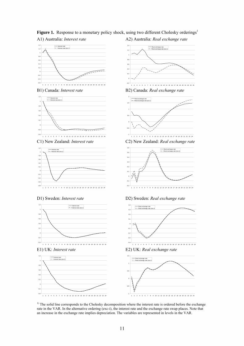
Figure 1. Response to a monetary policy shock, using two different Cholesky orderings1 A1) Australia: Interest rate A2) Australia: Real exchange rate
-0.6
-0.4
-0.2
0
0.2
0.4
0.6
0.8
1
1.2
1.4
1 2 3 4 5 6 7 8 9 10 11 12 13 14 15 16 17 18 19 20 21 22 23 24
Interest rateInterest rate (exc-i)
-0.2
0
0.2
0.4
0.6
0.8
1
1.2
1.4
1 2 3 4 5 6 7 8 9 10 11 12 13 14 15 16 17 18 19 20 21 22 23 24
Real exchange rateReal exchange rate (exc-i)
B1) Canada: Interest rate B2) Canada: Real exchange rate
-0.4
-0.2
0
0.2
0.4
0.6
0.8
1
1.2
1 2 3 4 5 6 7 8 9 10 11 12 13 14 15 16 17 18 19 20 21 22 23 24
Interest rateInterest rate (exc-i)
-1
-0.5
0
0.5
1
1.5
2
1 2 3 4 5 6 7 8 9 10 11 12 13 14 15 16 17 18 19 20 21 22 23 24
Real exchange rateReal exchange rate (exc-i)
C1) New Zealand: Interest rate C2) New Zealand: Real exchange rate
-0.8
-0.6
-0.4
-0.2
0
0.2
0.4
0.6
0.8
1
1.2
1 2 3 4 5 6 7 8 9 10 11 12 13 14 15 16 17 18 19 20 21 22 23 24
Interest rateInterest rate (exc-i)
-0.2
-0.1
0
0.1
0.2
0.3
0.4
0.5
0.6
1 2 3 4 5 6 7 8 9 10 11 12 13 14 15 16 17 18 19 20 21 22 23 24
Real exchange rateReal exchange rate (exc-i)
D1) Sweden: Interest rate D2) Sweden: Real exchange rate
-0.4
-0.2
0
0.2
0.4
0.6
0.8
1
1.2
1 2 3 4 5 6 7 8 9 10 11 12 13 14 15 16 17 18 19 20 21 22 23 24
Interest rateInterest rate (exc-i)
-0.4
-0.3
-0.2
-0.1
0
0.1
0.2
0.3
0.4
1 2 3 4 5 6 7 8 9 10 11 12 13 14 15 16 17 18 19 20 21 22 23 24
Real exchange rateReal exchange rate (exc-i)
E1) UK: Interest rate E2) UK: Real exchange rate
-0.4
-0.2
0
0.2
0.4
0.6
0.8
1
1.2
1 2 3 4 5 6 7 8 9 10 11 12 13 14 15 16 17 18 19 20 21 22 23 24
Interest rateInterest rate (exc-i)
-1
-0.5
0
0.5
1
1.5
1 2 3 4 5 6 7 8 9 10 11 12 13 14 15 16 17 18 19 20 21 22 23 24
Real exchange rate Real exchange rate (exc-i)
1) The solid line corresponds to the Cholesky decomposition where the interest rate is ordered before the exchange rate in the VAR. In the alternative ordering (exc-i), the interest rate and the exchange rate swap places. Note that an increase in the exchange rate implies depreciation. The variables are represented in levels in the VAR.
11
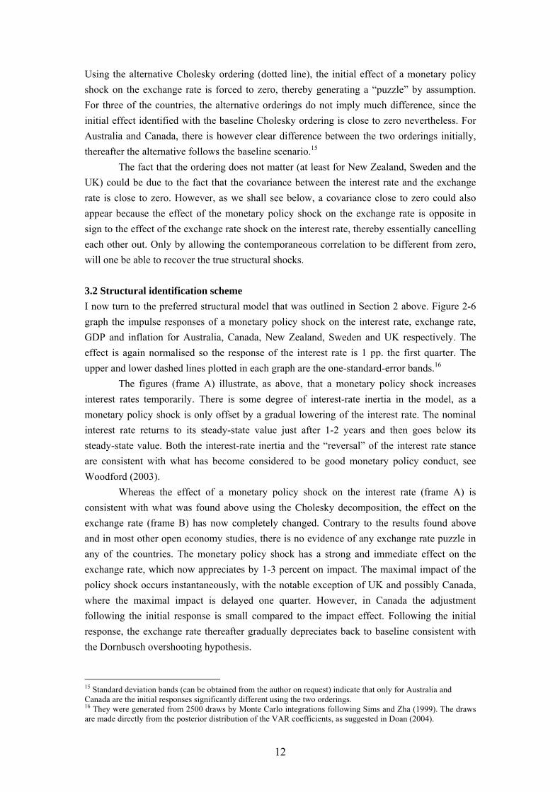
Using the alternative Cholesky ordering (dotted line), the initial effect of a monetary policy shock on the exchange rate is forced to zero, thereby generating a “puzzle” by assumption. For three of the countries, the alternative orderings do not imply much difference, since the initial effect identified with the baseline Cholesky ordering is close to zero nevertheless. For Australia and Canada, there is however clear difference between the two orderings initially, thereafter the alternative follows the baseline scenario.15 The fact that the ordering does not matter (at least for New Zealand, Sweden and the UK) could be due to the fact that the covariance between the interest rate and the exchange rate is close to zero. However, as we shall see below, a covariance close to zero could also appear because the effect of the monetary policy shock on the exchange rate is opposite in sign to the effect of the exchange rate shock on the interest rate, thereby essentially cancelling each other out. Only by allowing the contemporaneous correlation to be different from zero, will one be able to recover the true structural shocks. 3.2 Structural identification scheme I now turn to the preferred structural model that was outlined in Section 2 above. Figure 2-6 graph the impulse responses of a monetary policy shock on the interest rate, exchange rate, GDP and inflation for Australia, Canada, New Zealand, Sweden and UK respectively. The effect is again normalised so the response of the interest rate is 1 pp. the first quarter. The upper and lower dashed lines plotted in each graph are the one-standard-error bands.16 The figures (frame A) illustrate, as above, that a monetary policy shock increases interest rates temporarily. There is some degree of interest-rate inertia in the model, as a monetary policy shock is only offset by a gradual lowering of the interest rate. The nominal interest rate returns to its steady-state value just after 1-2 years and then goes below its steady-state value. Both the interest-rate inertia and the “reversal” of the interest rate stance are consistent with what has become considered to be good monetary policy conduct, see Woodford (2003).
Whereas the effect of a monetary policy shock on the interest rate (frame A) is consistent with what was found above using the Cholesky decomposition, the effect on the exchange rate (frame B) has now completely changed. Contrary to the results found above and in most other open economy studies, there is no evidence of any exchange rate puzzle in any of the countries. The monetary policy shock has a strong and immediate effect on the exchange rate, which now appreciates by 1-3 percent on impact. The maximal impact of the policy shock occurs instantaneously, with the notable exception of UK and possibly Canada, where the maximal impact is delayed one quarter. However, in Canada the adjustment following the initial response is small compared to the impact effect. Following the initial response, the exchange rate thereafter gradually depreciates back to baseline consistent with the Dornbusch overshooting hypothesis.
15 Standard deviation bands (can be obtained from the author on request) indicate that only for Australia and Canada are the initial responses significantly different using the two orderings. 16 They were generated from 2500 draws by Monte Carlo integrations following Sims and Zha (1999). The draws are made directly from the posterior distribution of the VAR coefficients, as suggested in Doan (2004).
12
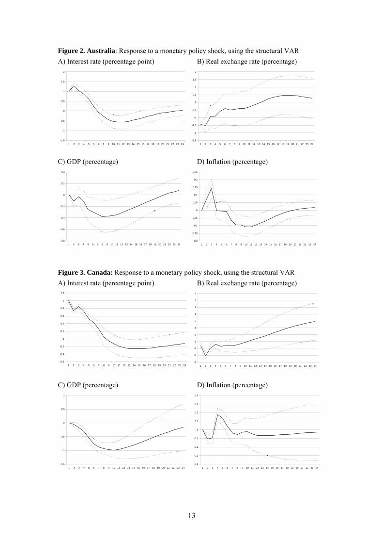
Figure 2. Australia: Response to a monetary policy shock, using the structural VAR A) Interest rate (percentage point) B) Real exchange rate (percentage)
-1.5
-1
-0.5
0
0.5
1
1.5
2
1 2 3 4 5 6 7 8 9 10 11 12 13 14 15 16 17 18 19 20 21 22 23 24-2.5
-2
-1.5
-1
-0.5
0
0.5
1
1.5
2
1 2 3 4 5 6 7 8 9 10 11 12 13 14 15 16 17 18 19 20 21 22 23 24
C) GDP (percentage) D) Inflation (percentage)
-0.8
-0.6
-0.4
-0.2
0
0.2
0.4
1 2 3 4 5 6 7 8 9 10 11 12 13 14 15 16 17 18 19 20 21 22 23 24-0.2
-0.15
-0.1
-0.05
0
0.05
0.1
0.15
0.2
0.25
1 2 3 4 5 6 7 8 9 10 11 12 13 14 15 16 17 18 19 20 21 22 23 24
Figure 3. Canada: Response to a monetary policy shock, using the structural VAR A) Interest rate (percentage point) B) Real exchange rate (percentage)
-0.6
-0.4
-0.2
0
0.2
0.4
0.6
0.8
1
1.2
1 2 3 4 5 6 7 8 9 10 11 12 13 14 15 16 17 18 19 20 21 22 23 24 -6
-5
-4
-3
-2
-1
0
1
2
3
4
1 2 3 4 5 6 7 8 9 10 11 12 13 14 15 16 17 18 19 20 21 22 23 24 C) GDP (percentage) D) Inflation (percentage)
-1.5
-1
-0.5
0
0.5
1
1 2 3 4 5 6 7 8 9 10 11 12 13 14 15 16 17 18 19 20 21 22 23 24 -0.4
-0.3
-0.2
-0.1
0
0.1
0.2
0.3
0.4
1 2 3 4 5 6 7 8 9 10 11 12 13 14 15 16 17 18 19 20 21 22 23 24
13
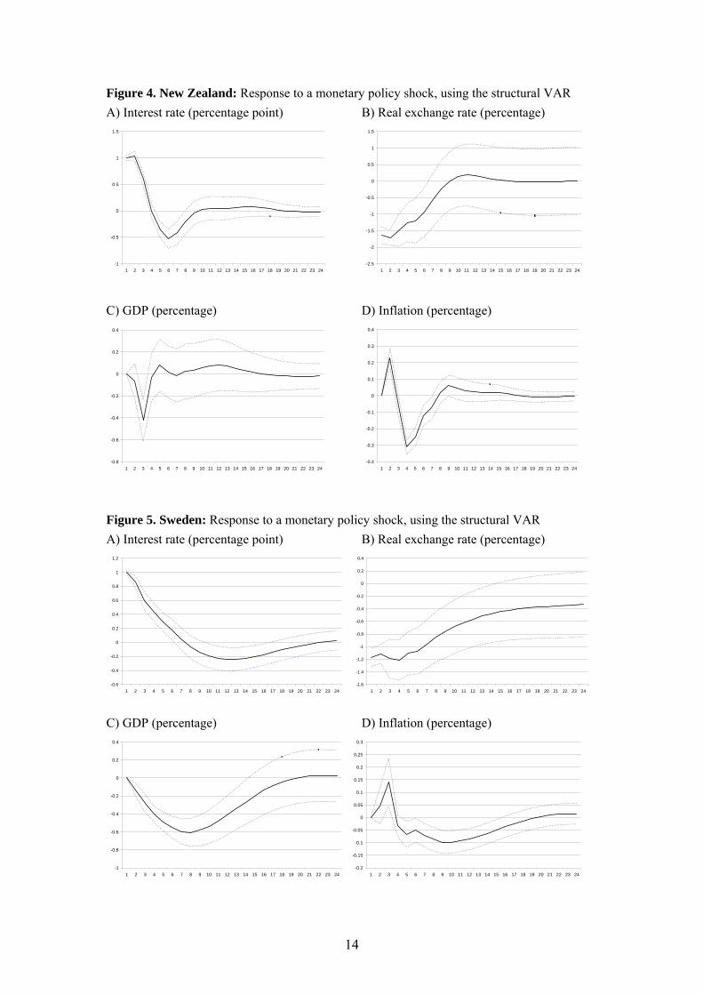
Figure 4. New Zealand: Response to a monetary policy shock, using the structural VAR A) Interest rate (percentage point) B) Real exchange rate (percentage)
-1
-0.5
0
0.5
1
1.5
1 2 3 4 5 6 7 8 9 10 11 12 13 14 15 16 17 18 19 20 21 22 23 24 -2.5
-2
-1.5
-1
-0.5
0
0.5
1
1.5
1 2 3 4 5 6 7 8 9 10 11 12 13 14 15 16 17 18 19 20 21 22 23 24 C) GDP (percentage) D) Inflation (percentage)
-0.8
-0.6
-0.4
-0.2
0
0.2
0.4
1 2 3 4 5 6 7 8 9 10 11 12 13 14 15 16 17 18 19 20 21 22 23 24 -0.4
-0.3
-0.2
-0.1
0
0.1
0.2
0.3
0.4
1 2 3 4 5 6 7 8 9 10 11 12 13 14 15 16 17 18 19 20 21 22 23 24 Figure 5. Sweden: Response to a monetary policy shock, using the structural VAR A) Interest rate (percentage point) B) Real exchange rate (percentage)
-0.6
-0.4
-0.2
0
0.2
0.4
0.6
0.8
1
1.2
1 2 3 4 5 6 7 8 9 10 11 12 13 14 15 16 17 18 19 20 21 22 23 24 -1.6
-1.4
-1.2
-1
-0.8
-0.6
-0.4
-0.2
0
0.2
0.4
1 2 3 4 5 6 7 8 9 10 11 12 13 14 15 16 17 18 19 20 21 22 23 24
C) GDP (percentage) D) Inflation (percentage)
-1
-0.8
-0.6
-0.4
-0.2
0
0.2
0.4
1 2 3 4 5 6 7 8 9 10 11 12 13 14 15 16 17 18 19 20 21 22 23 24-0.2
-0.15
-0.1
-0.05
0
0.05
0.1
0.15
0.2
0.25
0.3
1 2 3 4 5 6 7 8 9 10 11 12 13 14 15 16 17 18 19 20 21 22 23 24
14
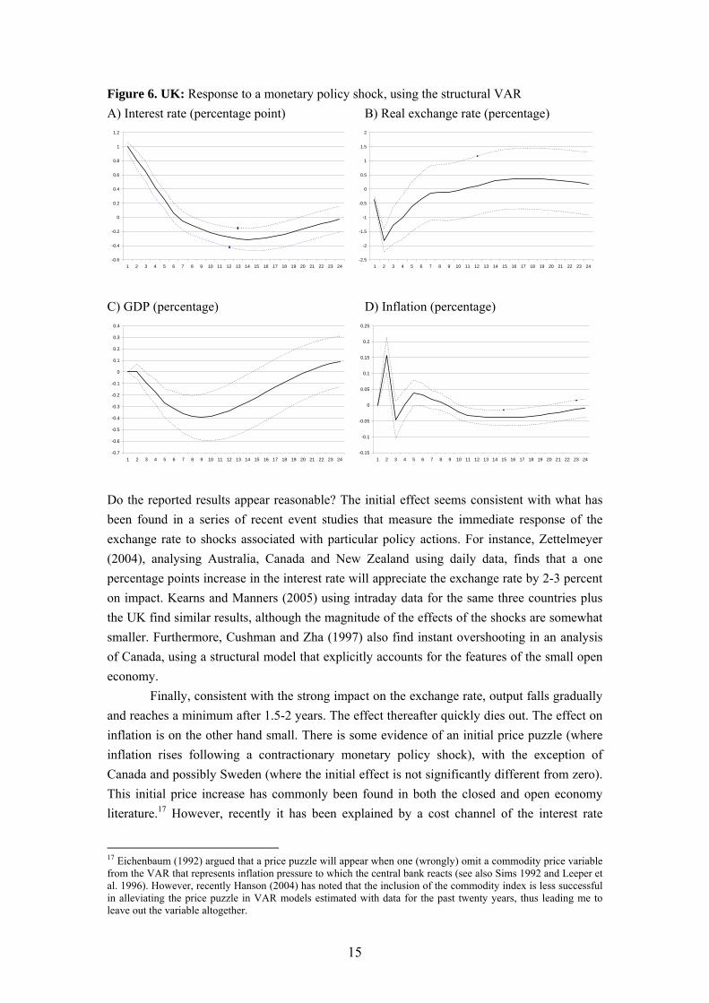
Figure 6. UK: Response to a monetary policy shock, using the structural VAR A) Interest rate (percentage point) B) Real exchange rate (percentage)
-0.6
-0.4
-0.2
0
0.2
0.4
0.6
0.8
1
1.2
1 2 3 4 5 6 7 8 9 10 11 12 13 14 15 16 17 18 19 20 21 22 23 24 -2.5
-2
-1.5
-1
-0.5
0
0.5
1
1.5
2
1 2 3 4 5 6 7 8 9 10 11 12 13 14 15 16 17 18 19 20 21 22 23 24 C) GDP (percentage) D) Inflation (percentage)
-0.7
-0.6
-0.5
-0.4
-0.3
-0.2
-0.1
0
0.1
0.2
0.3
0.4
1 2 3 4 5 6 7 8 9 10 11 12 13 14 15 16 17 18 19 20 21 22 23 24 -0.15
-0.1
-0.05
0
0.05
0.1
0.15
0.2
0.25
1 2 3 4 5 6 7 8 9 10 11 12 13 14 15 16 17 18 19 20 21 22 23 24
Do the reported results appear reasonable? The initial effect seems consistent with what has been found in a series of recent event studies that measure the immediate response of the exchange rate to shocks associated with particular policy actions. For instance, Zettelmeyer (2004), analysing Australia, Canada and New Zealand using daily data, finds that a one percentage points increase in the interest rate will appreciate the exchange rate by 2-3 percent on impact. Kearns and Manners (2005) using intraday data for the same three countries plus the UK find similar results, although the magnitude of the effects of the shocks are somewhat smaller. Furthermore, Cushman and Zha (1997) also find instant overshooting in an analysis of Canada, using a structural model that explicitly accounts for the features of the small open economy. Finally, consistent with the strong impact on the exchange rate, output falls gradually and reaches a minimum after 1.5-2 years. The effect thereafter quickly dies out. The effect on inflation is on the other hand small. There is some evidence of an initial price puzzle (where inflation rises following a contractionary monetary policy shock), with the exception of Canada and possibly Sweden (where the initial effect is not significantly different from zero). This initial price increase has commonly been found in both the closed and open economy literature.17 However, recently it has been explained by a cost channel of the interest rate
17 Eichenbaum (1992) argued that a price puzzle will appear when one (wrongly) omit a commodity price variable from the VAR that represents inflation pressure to which the central bank reacts (see also Sims 1992 and Leeper et al. 1996). However, recently Hanson (2004) has noted that the inclusion of the commodity index is less successful in alleviating the price puzzle in VAR models estimated with data for the past twenty years, thus leading me to leave out the variable altogether.
15
(where the increased interest rate increases borrowing costs for firms and therefore prices) and is less of a problem (see Ravenna and Walsh, 2003; Chowdhury et al., 2003).18 The effect on inflation is eventually significantly negative as expected, and peaks after 2-3 years. 3.3 Do Central Banks respond to exchange rate movements? I next turn to examine whether there is any (systematic) monetary policy response to exchange rate changes. That is, I examine the impulse responses for interest rates following an exchange rate shock. If monetary policy reacts immediately to exchange rate variation, then one would expect the interaction between interest rates and exchange rates to be important when identifying monetary policy shocks. If, on the other hand, no response is present, this might justify a zero contemporaneous restriction on the interest rate response, as has been done in many recent VAR studies. From the impulse responses (see appendix B), I find that an exchange rate shock that depreciates the exchange rate leads to a significant response in the interest rate in all countries. The effect is largest in Canada and smallest in the UK, where a shock that depreciates the exchange rate with one percent increases the interest rate with 0.36 and 0.08 percentage points respectively. Following the maximum response, the effect quickly dies out and only in Canada is the effect significant after a year.19
These results clearly illustrate that monetary policy responds systematically to exchange rate movements in all countries, but most notably so in Canada. This is consistent with what has been found in other part of the literature. For instance, Lubik and Schorfheide (2003) use bayesian techniques when estimating a small open structural economy model to examine whether Australia, Canada, New Zealand and the UK respond to exchange rate movements. They find that in all countries - and particular in Canada - does the interest rate increase following an exchange rate depreciation.20 Table 1 below provides a further answer by quantifying the contribution of the different shocks to the variance in the relevant variables. That is, the first row in Table 1 shows the variance decomposition of the real exchange rate with respect to the monetary policy shocks for all five countries. In the second row in table 1, I show the variance decomposition of the interest rates with respect to the exchange rate shocks for the same countries. Table 1 emphasize the variance decomposition for the first quarter where the maximum impact occurs, with the exception of Canada and the UK where the maximum impact is in the second quarter.
18 Using annual changes instead of quarterly changes in prices as the inflation measure, also reduces the price puzzle somewhat, see the discussion in section four below. 19 These responses might be motivated both by the central banks concern about reducing the impact of the shock on aggregate demand by conducting a policy that will offset the exchange rate effects, but also by reducing the exchange rate shock’s impact on exchange rate themselves – thereby diminishing the source of the problem. 20 That said, a posterior odds ratio also suggests that only in Canada (and possible UK) is an interest rate specification that allows for an exchange rate response preferred to one where the interest rate do not respond to exchange rate changes. However, a well known finding in the Bayesian literature (Lindley paradox) suggests that the null hypothesis (of no exchange rate response) will always be accepted when the variance of a conjugate prior goes to infinity. As the paper specifies a rather diffuse prior for the exchange rate, in more countries than what is reported could an interest rate response to exchange rate changes therefore potentially be preferred.
16
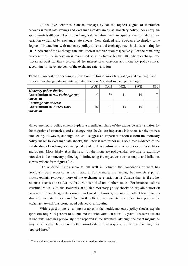
Of the five countries, Canada displays by far the highest degree of interaction between interest rate settings and exchange rate dynamics, as monetary policy shocks explain approximately 40 percent of the exchange rate variation, with an equal amount of interest rate variation explained by exchange rate shocks. New Zealand and Sweden also display some degree of interaction, with monetary policy shocks and exchange rate shocks accounting for 10-15 percent of the exchange rate and interest rate variation respectively. For the remaining two countries, the interaction is more modest, in particular for the UK, where exchange rate shocks account for three percent of the interest rate variation and monetary policy shocks accounting for seven percent of the exchange rate variation. Table 1. Forecast error decomposition: Contribution of monetary policy- and exchange rate shocks to exchange rate and interest rate variation. Maximal impact, percentage. AUS CAN NZL SWE UKMonetary policy shocks; Contribution to real exchange rate variation
5
39
11
14
7
Exchange rate shocks; Contribution to interest rates variation
16
41
10
15
3
Hence, monetary policy shocks explain a significant share of the exchange rate variation for the majority of countries, and exchange rate shocks are important indicators for the interest rate setting. However, although the table suggest an important response from the monetary policy maker to exchange rate shocks, the interest rate response is no direct evidence of the stabilization of exchange rate independent of the less controversial objectives such as inflation and output. More likely, it is the result of the monetary policymaker reacting to exchange rates due to the monetary policy lag in influencing the objectives such as output and inflation, as was evident from figures 2-6.
The reported results seem to fall well in between the boundaries of what has previously been reported in the literature. Furthermore, the finding that monetary policy shocks explain relatively more of the exchange rate variation in Canada than in the other countries seems to be a feature that again is picked up in other studies. For instance, using a structural VAR, Kim and Roubini (2000) find monetary policy shocks to explain almost 60 percent of the exchange rate variation in Canada. However, whereas the effect found here is almost immediate, in Kim and Roubini the effect is accumulated over close to a year, as the exchange rate exhibits pronounced delayed overshooting.
With regard to the remaining variables in the model, monetary policy shocks explain approximately 5-15 percent of output and inflation variation after 1-3 years. These results are in line with what has previously been reported in the literature, although the exact magnitude may be somewhat larger due to the considerable initial response in the real exchange rate reported here.21
21 These variance decompositions can be obtained from the author on request.
17
3.4 Uncovered interest parity (UIP) Having asserted that the exchange rate behaviour is consistent with Dornbusch overshooting in qualitatively terms, I finally turn to examine whether the subsequent response in the exchange rate is consistent with UIP. If UIP holds following a contractionary monetary policy
shock, the fall in the interest rate differential will be offset by an expected
depreciation of the exchange rate between time t and t+1. To explore this issue in more detail, I follow Eichenbaum and Evans (1995) and define Ψt as the ex post difference in return between holding one period foreign or domestic bonds. Measured in domestic currency, excess return is then given by:
*( - )t ti i
*
1- 4*( - )t t t t ti i s sψ += + , (6)
where st is the nominal exchange rate and st+1 is the forecasted three-month ahead exchange rate response.22 One implication of UIP is that the conditional expectations of the excess return should be zero:
0t t jEψ + = (7)
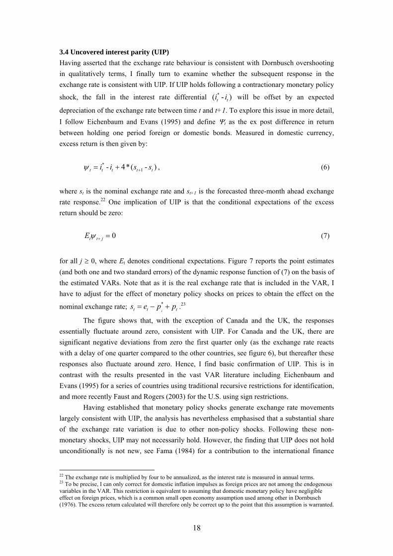
for all j ≥ 0, where Et denotes conditional expectations. Figure 7 reports the point estimates (and both one and two standard errors) of the dynamic response function of (7) on the basis of the estimated VARs. Note that as it is the real exchange rate that is included in the VAR, I have to adjust for the effect of monetary policy shocks on prices to obtain the effect on the
nominal exchange rate; .23 *tt ts e p p= − + t
The figure shows that, with the exception of Canada and the UK, the responses essentially fluctuate around zero, consistent with UIP. For Canada and the UK, there are significant negative deviations from zero the first quarter only (as the exchange rate reacts with a delay of one quarter compared to the other countries, see figure 6), but thereafter these responses also fluctuate around zero. Hence, I find basic confirmation of UIP. This is in contrast with the results presented in the vast VAR literature including Eichenbaum and Evans (1995) for a series of countries using traditional recursive restrictions for identification, and more recently Faust and Rogers (2003) for the U.S. using sign restrictions. Having established that monetary policy shocks generate exchange rate movements largely consistent with UIP, the analysis has nevertheless emphasised that a substantial share of the exchange rate variation is due to other non-policy shocks. Following these non-monetary shocks, UIP may not necessarily hold. However, the finding that UIP does not hold unconditionally is not new, see Fama (1984) for a contribution to the international finance
22 The exchange rate is multiplied by four to be annualized, as the interest rate is measured in annual terms. 23 To be precise, I can only correct for domestic inflation impulses as foreign prices are not among the endogenous variables in the VAR. This restriction is equivalent to assuming that domestic monetary policy have negligible effect on foreign prices, which is a common small open economy assumption used among other in Dornbusch (1976). The excess return calculated will therefore only be correct up to the point that this assumption is warranted.
18
literature and Engel (1996) for survey. That said, the policymaker should take great stride in the knowledge that conditioned on monetary policy, UIP will hold, which is the relevant policy question to examine. Figure 7 Excess returns A) Australia B) Canada
-3
-2
-1
0
1
2
3
1 2 3 4 5 6 7 8 9 10 11 12 13 14 15 16 17 18 19 20 -4
-3
-2
-1
0
1
2
3
4
1 2 3 4 5 6 7 8 9 10 11 12 13 14 15 16 17 18 19 20 C) New Zealand D) Sweden
-2
-1.5
-1
-0.5
0
0.5
1
1.5
2
1 2 3 4 5 6 7 8 9 10 11 12 13 14 15 16 17 18 19 20 -2
-1.5
-1
-0.5
0
0.5
1
1.5
1 2 3 4 5 6 7 8 9 10 11 12 13 14 15 16 17 18 19 20 E) UK
-6
-5
-4
-3
-2
-1
0
1
2
3
1 2 3 4 5 6 7 8 9 10 11 12 13 14 15 16 17 18 19 20
4 Robustness of results The robustness of the results reported above deserves further discussion on at least three issues with regard to specification: (i) Additional lags in the VAR, (ii) sample stability and (iii) choice of variables in the VAR. Below the results are presented with regard to the effect on the real exchange rate only, although where relevant, results for the other variables will be discussed. Impulse responses for all variables can be obtained from the author on request. 4.1 Specification - lags When testing for lag reduction in the structural model, most models could be reduced to three lags, although reducing the VAR further to two lags could not be supported. However, in many of the cases test diagnostics were quite similar using either three or four lags, and to check the robustness of the results with regard to lag selections, all models were therefore re-estimated using now four lags. The results of a contractionary monetary policy shock (that
19

increase the interest rate with 1 pp on impact) on the exchange rate are presented in Frame A in Figure 8 below. In each diagram, the baseline results using three lags (solid line) is plotted together with the alternative of four lags (dotted lines). Overall, the main results still prevail, although the exact magnitude of the effects of shocks has changed somewhat. In particular, for Sweden the impact effect is larger initially than in the baseline, but then declines in line with the baseline back to equilibrium. However, there is still no evidence of an exchange rate puzzle in any countries, as the exchange rate appreciates on impact, and thereafter (within a quarter) depreciates gradually and smoothly back to equilibrium. 4.2 Sample stability To check for robustness with respect to sample stability, all models were re-estimated shifting the start date first back and then forwards with five years; 1978-2004 and 1988-2004. Although convenient dates due to the five year interval, the dates are not chosen randomly. The start date for the extended sample (1978) reflects the earliest start date common to all countries.24 The start date for the more recent sample (1988) is chosen for two reasons. First, from 1988, price stability has been a more explicit focus in many countries; starting with Canada and New Zealand first referring to the desirability of inflation targeting in 1988 and with the others countries subsequently following (see Collins and Siklos, 2004, and the references stated therein).25 Second and probably related to the first, Bagliano and Favero (1998) have found that with regard to mis-specification, starting the estimation in 1988 is preferred to that of 1983 when analysing monetary policy, although the impulse responses using the two different periods may not be statistically different.
The results are presented in Frame B in Figure 8. The solid line corresponds to the baseline scenario; the dotted line to the period starting in 1978; the semi dotted line to the period starting in 1988. Overall, the main conclusions prevail, as following a monetary policy shock the exchange rates appreciate on impact in all countries. However, in some countries, the maximal response is delayed a quarter using the sample starting in 1978, which is not surprising as monetary policy shocks are now identified on a large sample that could potentially be confounding different monetary policy regimes. However, the adjustment eventually following is small compared to the initial adjustment.
The results using the more recent sample are also generally very supportive of the above findings; no evidence of an exchange rate puzzle as the exchange rates appreciate on impact. For some countries the effect is even more pronounced, in particular for the UK where the maximum impact effect now comes the first quarter, indicating the importance of monetary policy shocks for exchange rate variation in more recent time.
24 For Canada, data were available back to 1973, and the results are robust also to this extended period. Note that for New Zealand I use annual changes in CPI for the period 1978-2004, as quarterly changes showed a large degree of volatility in the period when New Zealand changed from a closed and centrally controlled economy to one of the most open economies. For Sweden, the three month interest rate was only available to 1982. I therefore used the Call Money Rate prior to 1982, and included a dummy to link the two interest rate series. 25 For instance, in Australia, the aim at stabilising inflation had been included in the Bank's public statements for a number of years before formally adopted in 1993.
20
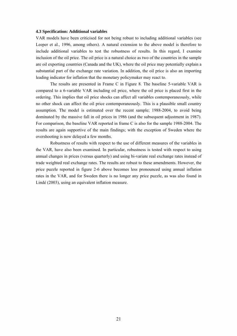
4.3 Specification: Additional variables VAR models have been criticised for not being robust to including additional variables (see Leeper et al., 1996, among others). A natural extension to the above model is therefore to include additional variables to test the robustness of results. In this regard, I examine inclusion of the oil price. The oil price is a natural choice as two of the countries in the sample are oil exporting countries (Canada and the UK), where the oil price may potentially explain a substantial part of the exchange rate variation. In addition, the oil price is also an importing leading indicator for inflation that the monetary policymaker may react to.
The results are presented in Frame C in Figure 8. The baseline 5-variable VAR is compared to a 6-variable VAR including oil price, where the oil price is placed first in the ordering. This implies that oil price shocks can affect all variables contemporaneously, while no other shock can affect the oil price contemporaneously. This is a plausible small country assumption. The model is estimated over the recent sample; 1988-2004, to avoid being dominated by the massive fall in oil prices in 1986 (and the subsequent adjustment in 1987). For comparison, the baseline VAR reported in frame C is also for the sample 1988-2004. The results are again supportive of the main findings; with the exception of Sweden where the overshooting is now delayed a few months.
Robustness of results with respect to the use of different measures of the variables in the VAR, have also been examined. In particular, robustness is tested with respect to using annual changes in prices (versus quarterly) and using bi-variate real exchange rates instead of trade weighted real exchange rates. The results are robust to these amendments. However, the price puzzle reported in figure 2-6 above becomes less pronounced using annual inflation rates in the VAR, and for Sweden there is no longer any price puzzle, as was also found in Lindé (2003), using an equivalent inflation measure.
21
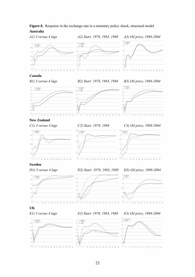
Figure 8. Response in the exchange rate to a monetary policy shock, structural model Australia A1) 3 versus 4 lags A2) Start: 1978, 1983, 1988 A3) Oil price, 1988-2004
-2
-1.5
-1
-0.5
0
0.5
1
1 4 7 10 13 16 19 22 25 28 31 34 37 40
Baseline4 lags
-4
-3
-2
-1
0
1
2
1 4 7 10 13 16 19 22 25 28 31 34 37 40
Baseline19781988
-4
-3
-2
-1
0
1
2
1 4 7 10 13 16 19 22 25 28 31 34 37 40
BaselineOILP
Canada B1) 3 versus 4 lags B2) Start: 1978, 1983, 1988 B3) Oil price, 1988-2004
-6
-5
-4
-3
-2
-1
0
1
2
1 4 7 10 13 16 19 22 25 28 31 34 37 40
Baseline4 lags
-6
-5
-4
-3
-2
-1
0
1
1 4 7 10 13 16 19 22 25 28 31 34 37 40
Baseline19781988
-7
-6
-5
-4
-3
-2
-1
0
1
2
1 4 7 10 13 16 19 22 25 28 31 34 37 40
BaselineOILP
New Zealand C1) 3 versus 4 lags C2) Start: 1978, 1988 C3) Oil price, 1988-2004
-2
-1.5
-1
-0.5
0
0.5
1
1 4 7 10 13 16 19 22 25 28 31 34 37 40
Baseline4 lags
-2
-1.5
-1
-0.5
0
0.5
1 4 7 10 13 16 19 22 25 28 31 34 37 40
Baseline1978
-2.5
-2
-1.5
-1
-0.5
0
0.5
1 4 7 10 13 16 19 22 25 28 31 34 37 40
BaselineOILP
Sweden D1) 3 versus 4 lags D2) Start: 1978, 1983, 1988 D3) Oil price, 1988-2004
-3
-2.5
-2
-1.5
-1
-0.5
0
1 4 7 10 13 16 19 22 25 28 31 34 37 40
Baseline4 lags
-1.4
-1.2
-1
-0.8
-0.6
-0.4
-0.2
0
1 4 7 10 13 16 19 22 25 28 31 34 37 40
-2
-1.5
-1
-0.5
0
0.5
1
1 4 7 10 13 16 19 22 25 28 31 34 37 40
BaselineOILP
UK E1) 3 versus 4 lags E2) Start: 1978, 1983, 1988 E3) Oil price, 1988-2004
-2.5
-2
-1.5
-1
-0.5
0
0.5
1
1 4 7 10 13 16 19 22 25 28 31 34 37 40
Baseline4 lags
-2
-1.5
-1
-0.5
0
0.5
1
1.5
2
1 4 7 10 13 16 19 22 25 28 31 34 37 40
Baseline19781988
-2
-1.5
-1
-0.5
0
0.5
1
1.5
2
1 4 7 10 13 16 19 22 25 28 31 34 37 40
Baseline-UKOILP
22
5 Concluding remarks Dornbusch’s (1976) well known exchange rate overshooting is a central building block in international macroeconomics, stating that the nominal exchange rate immediately appreciates with the increase in nominal interest rates, in line with uncovered interest parity (UIP). When confronted with data, however, very few empirical studies analysing the effects of monetary policy shocks have found support for Dornbusch overshooting. Instead they have found that following a contractionary monetary policy shock, the real exchange rate either depreciates, or, if it appreciates, it does so for a prolonged period of up to three years, thereby giving a hump-shaped response that violates UIP. From a theoretical point of view, these results are surprising. Delay appreciation after an interest rate hike may involve “money on the table”, as agents may benefit from both higher interest rates and appreciation of the exchange rate. Yet, these results have been so pervasive that the puzzles themselves are now about to be considered consensus, of which many recently developed DSGE models seek to replicate.
The majority of studies quantifying the effects of monetary policy shocks have used the vector autoregressive (VAR) approach. A major problem facing these studies is how to address the simultaneity of monetary policy and the exchange rate. Most of the studies of open economies are placing zero contemporaneous restrictions on the response of the systematic interest rate setting to an exchange rate shock, or vice versa. However, this is not consistent with established theory neither on monetary policy nor on exchange rate determination. Furthermore, Faust and Rogers (2003) have recently shown that the delayed overshooting feature of the open economy VAR is very sensitive to this kind of restriction. VAR models of the open economy should therefore seek to identify monetary policy without restricting the contemporaneous response.
This paper suggests an alternative identification that restricts the long run multipliers of the shocks, but with no restriction on the contemporaneous relationship between the interest rate and the exchange rate. Identification is achieved by assuming that monetary policy shocks can have no long run effect on the level of the real exchange rate. This is a standard neutrality assumption that holds for a large class of models in the monetary policy literature. In the short run, however, monetary policy is free to influence the exchange rate.
Allowing for full simultaneity between monetary policy and the exchange rate, I find striking results; Contrary to the recent “consensus”, a contractionary monetary policy shock has a strong effect on the exchange rate that appreciates on impact. The maximal impact occurs immediately, and the exchange rate thereafter gradually depreciates back to baseline. This is consistent with the Dornbusch overshooting hypothesis. Furthermore, the ensuing movement of the exchange rate is with few exceptions consistent with UIP. Hence, I have found no evidence of the typical hump-shaped response found in the empirical literature (i.e. Eichenbaum and Evans, 1995). Instead I find renewed support for the view that policy shocks generate exchange rate responses consistent with UIP.
Furthermore, the qualitative properties of a monetary policy with regard to domestic variables that have been found in the established literature still hold. In particular, a contractionary policy shock temporarily lowers output and has a sluggish but eventually negative effect on consumer price inflation.
23
References Adolfson, M., Laséen, S., Lindé J., and M. Villani (2006), “Evaluating An Estimated New Keynesian Small Open Economy Model,” Manuscript, Sveriges Riksbank. Bagliano, F.C. and C.A. Favero (1998), “Measuring monetary policy with VAR models: An evaluation,” European Economic Review, 42, 1069-1112. Bjørnland, H.C. (2005), “Monetary Policy and Exchange Rate Interactions in a Small Open Economy,” Manuscript, University of Oslo. Bjørnland, H.C. and K. Leitemo (2004), “Identifying the Interdependence between US Monetary Policy and the Stock Market,” Manuscript, University of Oslo. Bonser-Neal, C., V.V. Roley and G.H. Sellon, Jr. (1998), “Monetary Policy Actions, Intervention, and Exchange Rates: A Reexamination of the Empirical Relationships Using Federal Funds Rate Target Data,” Journal of Business, 71, pp. 147-177. Blanchard, O. and D. Quah (1989), “The Dynamic Effects of Aggregate Demand and Supply Disturbances,” American Economic Review, 79, 655-73. Christiano, L.J., Eichenbaum, M. and C.L. Evans (1999), “Monetary Policy Shocks: What Have we Learned and to What End?,” in J.B. Taylor and M. Woodford, eds., Handbook of Macroeconomics. Volume 1A. New York: Elsevier Science, 65-148. Christiano, L., Eichenbaum, M. and C.L. Evans (2005), “Nominal Rigidities and the Dynamic Effects of a Shock to Monetary Policy,” Journal of Political Economy 113, 1-45. Chowdhury, I., Hoffmann, M. and A. Schabert (2003), “Inflation Dynamics and the Cost Channel of Monetary Transmission,” Manuscript University of Cologne. Clarida R. and J. Gali (1994), “Sources of real exchange rate fluctuations: how important are nominal shocks?” Carnegie-Rochester Conference Series on Public Policy, 41, 1-56. Clarida, R., J. Galí and M. Gertler (1998), “Monetary policy rules in practice: Some international evidence,” European Economic Review, 42, 1033-1067. Clarida, R., J. Gali and M. Gertler (2000), “Monetary policy rules and macroeconomic stability: evidence and some theory,” Quarterly Journal of Economics, 115, 147-180.
24
Clarida, R., J. Galí and M. Gertler (2001), “Optimal Monetary Policy in Open Versus Closed Economies: An Integrated Approach,” American Economic Review Papers and Proceeding, 91, 248-252. Collins, S. and P.L. Siklos (2004) “Optimal Monetary Policy Rules and Inflation Targets: Are Australia, Canada and New Zealand Different from the U.S.?” Open Economies Review 15, 347-362. Cushman, D.O. and T. Zha (1997), “Identifying monetary policy in a small open economy under flexible exchange rates,” Journal of Monetary Economics, 39, 433-448. Doan, Thomas (2004), Rats Manual, Version 6, Estima, Evanston, IL. Dornbusch, R. (1976), “Expectations and Exchange Rate Dynamics,” Journal of Political Economy, 84, 1161-1176. Eichenbaum, M. (1992), “Comment on Interpreting the macroeconomic time series facts: the effects of monetary policy,” European Economic Review, 36, 1001–1011. Eichenbaum, M. and C. Evans (1995), “Some empirical evidence on the effects of shocks to monetary policy on exchange rates,” Quarterly Journal of Economics, 110, 975-1010. Engel, C. (1996), “The forward discount anomaly and the risk premium: a survey of recent evidence,” Journal of Empirical Finance, 3, 123-191. Evans, L. A. Grimes and B. Wilkinson (1996), “Economic Reform in New Zealand 1984-95: The Pursuit of Efficiency,” Journal of Economic Literature, 34, 1856-1902. Fama, E.F. (1984), “Forward and Spot Exchange Rates,” Journal of Monetary Economics, 14, 319-338. Faust, J. and E.M. Leeper (1997), “When Do Long-Run Identifying Restrictions Give
Reliable Results? ” Journal of Business and Economic Statistics, 15, 345-353.
Faust, J. and J.H. Rogers (2003), “Monetary policy's role in exchange rate behaviour”, Journal of Monetary Economics, 50, 1403-1424. Faust, J., E.T. Swanson and J.H. Wright (2004), “Identifying VARS based on high frequency futures data”, Journal of Monetary Economics, 51, 1107-1131. Favero, C.A. and M. Marcellino (2004), “Large Datasets, Small Models and Monetary Policy in Europe”, Manuscript, Bocconi University.
25
Giordani, P. (2004), “An alternative explanation of the price puzzle”, Journal of Monetary Economics, 51, 1271-1296. Greenspan, A. (2005) “Reflections on central banking”, Symposium sponsored by the Federal Reserve Bank of Kansas City, Jackson Hole, Wyoming, August 26, 2005. Hamilton, J.D. (1994), Time Series Analysis, Princeton University Press, New Jersey. Hanson, M.S. (2004), “The “price puzzle” reconsidered,” Journal of Monetary Economics, 51, 1385-1413. Kearns, J. and P. Manners (2005) “The Impact of Monetary Policy on the Exchange Rate: A Study Using Intraday Data”, Reserve Bank of Australia Research Discussion Papers 2005-02. Kim, S. and N. Roubini (2000), “Exchange rate anomalies in the industrial countries: A solution with a structural VAR approach”, Journal of Monetary Economics, 45, 561-586. Lane, P.R. (2001), “The new open economy macroeconomics: a survey,” Journal of International Economics, 54, 235-266. Leeper, E.M., Sims, C.A. and T. Zha, (1996), “What does monetary policy do?” Brookings Papers on Economic Activity, 2, 1-78. Lindé, J. (2003), “Monetary Policy Shocks and Business Cycle Fluctuations in a Small Open Economy: Sweden 1986-2002”, Sveriges Riksbank Working Paper Series No.153. Lindé, J. M. Nessen and U. Söderström (2004), “Monetary Policy in an Estimated Open-Economy Model with Imperfect Pass-Through”, CEPR Discussion Paper No. 4531. Lubik, T.A. and F. Schorfheide (2003), “Do Central Banks Respond to Exchange Rate Movements? A Structural Investigation,” Manuscript, University of Pennsylvania. Mojon B. and G. Peersman (2003), “A VAR description of the effects of monetary policy in the individual countries of the Euro area,” In I. Angeloni, A. Kashyap and B. Mojon (eds), Monetary policy transmission in the Euro area, Cambridge University Press, Part 1, 56-74. Murchison, S., A. Rennison and Z. Zhu (2004), “A Structural Small Open-Economy Model for Canada,” Bank of Canada Working Paper 2004-4. Obstfeld, M. (1985), “Floating Exchange Rates: Experience and Prospects,” Brookings Papers on Economic Activity, 2, 369-450.
26
Obstfeld, M. and K. Rogoff (1995), “Exchange rate dynamics redux,” Journal of Political Economy, 103, 624-660. Obstfeld, M. and K. Rogoff (2000), “New Directions for Stochastic Open Economy Models,” Journal of International Economics, 50, 117-153. Peersman, G. and F. Smets (2003) “The monetary transmission mechanism in the euro area: more evidence from VAR analysis”, In I. Angeloni, A. Kashyap and B. Mojon (eds), Monetary Policy Transmission in the Euro Area, Cambridge University Press, Part 1, 36-55. Ravenna, F. and C.E. Walsh (2003), “The Cost channel in a New Keynesian Model: Evidence and Implications,” University of California, Santa Cruz. Rogoff, K. (2002), “Dornbusch’s Overshooting Model after Twenty-Five Years,” IMF Working Paper 02/39. Rudebusch, G.D. (1998), “Do Measures of Monetary Policy in a VAR Make Sense?” International Economic Review, 39, 907-931. Scholl, A. and H. Uhlig (2005), “New Evidence on the Puzzles. Results from Agnostic Identification on Monetary Policy and Exchange Rates,” Mimeo Humboldt University. Sims, C.A. (1980), “Macroeconomics and Reality,” Econometrica, 48, 1-48. Sims, C.A. (1992), “Interpreting the Macroeconomic Time Series Facts: The Effects of Monetary Policy,” European Economic Review, 36, 975-1011. Sims, C.A., J.H. Stock, and M.W. Watson (1990) “Inference in Linear Time Series Models with Some Unit Roots,” Econometrica, 58, 113-144. Sims, C.A. and T. Zha, (1999), “Error bands for impulse responses,” Econometrica, 67, 1113-1157. Smets, F. and R. Wouters (2002), “Openess, imperfect exchange rate pass-through and monetary policy,” Journal of Monetary Economics, 49, 947-981. Svensson, L.E.O. (1997), “Inflation Forecast Targeting: Implementing and Monitoring Inflation Targets,” European Economic Review 41, 1111-46. Svensson, L.E.O. (2000), “Open-Economy Inflation Targeting,” Journal of International Economics, 50, 155-183.
27
Taylor, J.B. (2001), “The role of the Exchange Rate in Monetary-Policy Rules,” American Economic Review, 91, 263-67. Woodford, M. (2003), “Optimal Interest-Rate Smoothing,” Review of Economic Studies, 70, 861-86. Zettelmeyer, J. (2004), “The impact of monetary policy on the exchange rate: evidence from three small open economies,” Journal of Monetary Economics, 51, 635-652.
28
Appendix A All data are taken from the OECD database, except the Fed Funds rate that is taken from Eco Win. GDP and inflation are seasonally adjusted (s.a) by the official sources, the remaining series are unadjusted. The following data series are used: (πt) Inflation, measured as quarterly changes in the consumer price index (CPI) except for UK where the harmonized CPI is used (the only series available s.a.) (yt) Log real GDP, deflated by the official sources (et) [CCRETT01.IXOB.Q] Log of the real effective exchange rate, measured against a basket of trading partners. The exchange rate is specified so that an increase implies depreciation. (it) [IR3TBB01.ST.Q] Three month domestic interest rate. (it*) Trade-weighted foreign interest rate. For Canada and the UK, the foreign interest rate is represented by the Federal Funds rate, as the US comprises more than 50 percent of the foreign trade weight.26 For Australia, New Zealand and Sweden, the foreign interest is an weighted average of the interest rate in the major trading partners, source: Reserve Bank of Australia (http://www.rba.gov.au/), Reserve Bank of New Zealand (http://www.rbnz.govt.nz/) and Sveriges Riksbank ( http://www.riksbank.com/) respectively
26 For Canada, more than 80 percent of its export goes to the US.
29
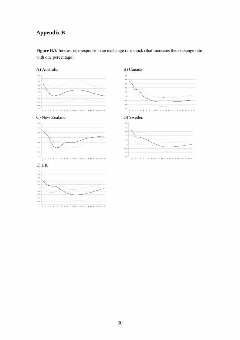
Appendix B Figure B.1. Interest rate response to an exchange rate shock (that increases the exchange rate with one percentage). A) Australia B) Canada
-0.08
-0.06
-0.04
-0.02
0
0.02
0.04
0.06
0.08
0.1
0.12
1 2 3 4 5 6 7 8 9 10 11 12 13 14 15 16 17 18 19 20 21 22 23 24 -0.3
-0.2
-0.1
0
0.1
0.2
0.3
0.4
0.5
1 2 3 4 5 6 7 8 9 10 11 12 13 14 15 16 17 18 19 20 21 22 23 24 C) New Zealand D) Sweden
-0.2
-0.15
-0.1
-0.05
0
0.05
0.1
0.15
1 2 3 4 5 6 7 8 9 10 11 12 13 14 15 16 17 18 19 20 21 22 23 24 -0.15
-0.1
-0.05
0
0.05
0.1
0.15
0.2
0.25
1 2 3 4 5 6 7 8 9 10 11 12 13 14 15 16 17 18 19 20 21 22 23 24 E) UK
-0.1
-0.08
-0.06
-0.04
-0.02
0
0.02
0.04
0.06
0.08
0.1
1 2 3 4 5 6 7 8 9 10 11 12 13 14 15 16 17 18 19 20 21 22 23 24
30