Module 2: Introduction to Statistics

Module 2: Introduction to Statistics

Niko Kaciroti, Ph.D.BIOINF 525 Module 2: W17

University of Michigan

Course Info• Instructor

– Niko Kaciroti: [email protected]• Office: 300 N. Ingalls Bldg, 10-floor, #1027NW• Office hours: Friday 11:00pm to 12:00pm or by appointment

• Teaching Assistant– Lauren Jepsen: [email protected]

• Office hours: Monday 12:00pm-1:00pm, Palmer 2065

• Data from TROPHY Study will be used for the class– Feasibility of treating prehypertension with an angiotensin-receptor

blocker. New England Journal of Medicine. 2006; 354:1685-97.

• Grading– Homework

• Students may form study groups to discuss class notes and homework assignments but must hand in their own work

mailto:[email protected]

mailto:[email protected]

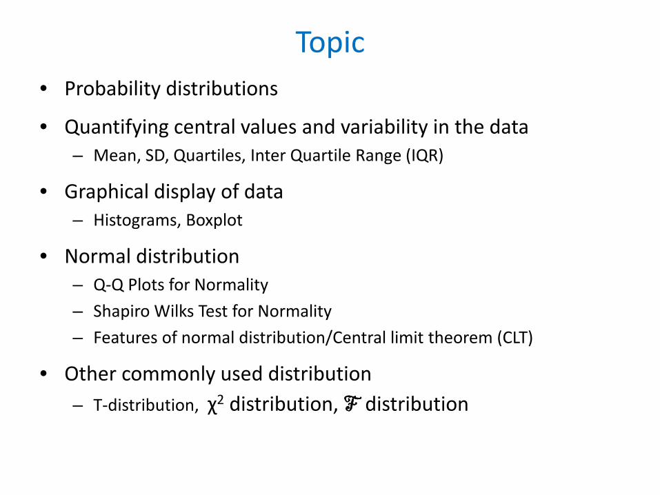
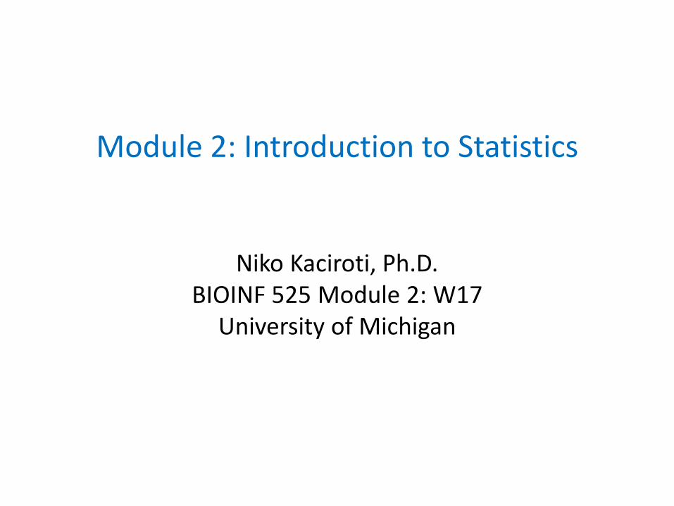
Topic• Probability distributions

• Quantifying central values and variability in the data– Mean, SD, Quartiles, Inter Quartile Range (IQR)

• Graphical display of data– Histograms, Boxplot

• Normal distribution – Q-Q Plots for Normality– Shapiro Wilks Test for Normality– Features of normal distribution/Central limit theorem (CLT)

• Other commonly used distribution– T-distribution, χ2 distribution, F distribution

Statistical Programs

• Some commonly used statistical programs:

– SAS– SPSS– Stata– R/Rstudio

• R is an open source program, and will be used in the lab. It is available for downloaded at: http://cran.r-project.org/Rstudio at: http://www.rstudio.com/ide/download/

• Reference Book : The R Book 2nd edition by Michael J. Crawley

http://cran.r-project.org/

http://www.rstudio.com/ide/download/

Variable Types

• Discrete variables (or categorical data)– May take values as an integer or belong to a set number

of categories # Number of sunny days in January (0,1,2,…,31) Gender (0=“Female”, 1=“Male”) Race (1=“White”, 2=“Black”, 3=“Asian”, 4=“Others”)

• Continuous variables– May take any real value within a defined range

Height/Weight (6.11ft,/191.12lbs) Blood Pressure (100.12mmHg)

Randomness and Probability

• The concepts of randomness and probability are central to the field of statistics

• Most experiments are not perfectly reproducible: some experiments are more accurate, some are less

• We will outline the basic ideas of probability distributions, which are used to measure the degree of uncertainty and reproducibility

Probability Distributions

• Probability distribution describes how data points are distributed. That is, what is the likelihood (or relative frequency) that a certain value occurs

• It is a mathematical function that assigns some probability to each of the possible outcome values of a random variable (X)† – Probability mass function (pmf): Is used for discrete variables– Probability density function (pdf): Is used for continuous variables

†X is a random variable if it can take different values, each with some probability. – E.g., X indicates the outcome of tossing a coin (Tail/Head).

PMF for Discrete Variables

• Pmf is a function that gives the probability that X equals to some value k, Pr(X=k).– E.g. Tossing a coin, the pmf is:

Pr(X=Tail)=p=0.5Pr(X=Head)=1-p=0.5

– Rolling a dice, the pmf is:Pr(X=k)=pk=1/6 for k=1,2,…,6.

– Sum of all probabilities must be 1:

�𝑘𝑘=1

𝑛𝑛

𝑃𝑃𝑟𝑟(𝑋𝑋 = 𝑘𝑘) = 1

PDF for Continuous Variables

• The probability density function f(x) is a bit more complicated when x is continuous. It is defined as the limit when δx → 0 of :

Pr(x≤X<x+δx) / δx = f(x)

Here Pr(x ≤ X<x+δx) is the probability that X lies between x and x+δx where δx is small

• Another useful function describing the distribution is the Cumulative Density Function (CDF), which gives the probability that X is less than or equal to x:

F(x)=P(X ≤ x)=∫−∞𝑥𝑥 𝑓𝑓 𝑥𝑥 𝑑𝑑𝑥𝑥

Why It’s Important to Learn About Different Distributions?

• It is necessary to decide which are the appropriate: – Descriptive measures (to best analyze/present the data)– Statistical test(s) when testing hypothesis

• Helps in deciding whether to transform your data – Does the data have characteristics that might make it

inconsistent with the assumptions about the distributions used in a statistical test?

Commonly Used Distributions(Continuous Variables)

• Normal distribution with mean μ and variance σ2

• t distribution with k degrees of freedom (aka Student's t distribution)

• Chi-Square (𝜒𝜒2) distribution with k degrees of freedom

• F distribution with (n, m) degrees of freedom– degrees of freedom (df) is the number of values in a statistics that

are free to vary (not constrained). – df=n-#of constrains

Normal, t, χ2, and F distributions are widely used for statistical testing (more on these later). These tests are derived based on normal distribution assumption, which makes the normal distribution vital to statistics.

Commonly Used Distributions(Discrete Variables)

• Bernoulli distribution (Yes/No)– Tossing a coin, does it land “Tail”: 1=“Yes”/0=“No”)

• Binomial distribution (Number of successes in n trials) – Number of “tails” when tossing a coin n times (e.g. 5 times out of 10)

• Multinomial distribution (belonging to some categories)– Race 1=W, 2=B, 3=A, 4=Other

• Poisson distribution (count data: 0,1,2,….)– # of goals is a soccer game (0,1,2,….)– # of points in a football game???






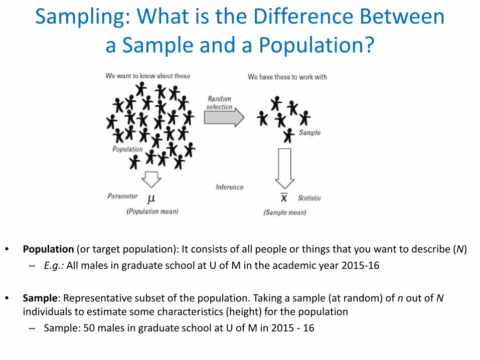
Sampling: What is the Difference Between a Sample and a Population?

• Population (or target population): It consists of all people or things that you want to describe (N)– E.g.: All males in graduate school at U of M in the academic year 2015-16

• Sample: Representative subset of the population. Taking a sample (at random) of n out of Nindividuals to estimate some characteristics (height) for the population– Sample: 50 males in graduate school at U of M in 2015 - 16

Sampling Example: Two samples of n=10 students

Sample 1 (height) Sample 2 (height)5.2 5.55.4 5.55.5 5.65.6 5.65.7 5.75.8 5.85.9 5.86.0 5.96.1 5.9

mean height 5.7 5.7What is different between sample 1 and sample 2?

– Sample 2 is more homogenous. All heights are within 2 inches from the mean.

Quantifying Central Values and Variability in the DataMean, Variance, Standard Deviation

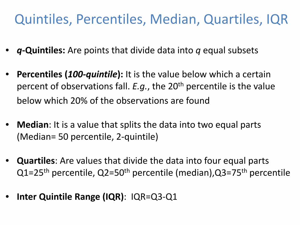
Quintiles, Percentiles, Median, Quartiles, IQR

• q-Quintiles: Are points that divide data into q equal subsets

• Percentiles (100-quintile): It is the value below which a certain percent of observations fall. E.g., the 20th percentile is the value below which 20% of the observations are found

• Median: It is a value that splits the data into two equal parts (Median= 50 percentile, 2-quintile)

• Quartiles: Are values that divide the data into four equal parts Q1=25th percentile, Q2=50th percentile (median),Q3=75th percentile

• Inter Quintile Range (IQR): IQR=Q3-Q1

Calculating Percentiles

Data Sorted(n=11)11 1135 1231 2224 2412 3057 3132 3230 3522 4477 5744 77Mean=32.3 SD=18

Q1

Median/Q2

Q3

The pth percentile of n values is the p*nth value in the sorted data (round to the nearest integer in the list 1,2,…,n of order)

Median: 0.5*11=5.5 (the 6th )→ 31

Q1: 0.25*11=2.75 (the 3rd) → 22

Q3: 0.75*11=8.25 (the 8th) → 44

IQR = Q3-Q1: 44-22=22

Calculating Percentiles(Not sensitive to outliers)

Data Sorted(n=11)11 1135 1231 2224 2412 3057 3132 3230 3522 4477 5744 777Mean=32.3 (96.9) SD=18 (215.4)

Q1

Median/Q2

Q3

Would the mean or median change if there was a large outlier?

Median: 0.5*11=5.5 (the 6th )→ 31

Q1: 0.25*11=2.75 (the 3rd) → 22

Q3: 0.75*11=8.25 (the 8th) → 44

IQR = Q3-Q1: 44-22=22






Graphical Display of Data

• A visual or graphical display of data is a useful tool for understanding and summarizing the data. It should alwaysbe the first step on statistical analysis.– It is very useful for data quality control, checking for errors,

unusual values or outliers– It is also useful for understanding the distributions of the data,

which will help in choosing the appropriate statistical models

• Two important graphical display of data are:– Histogram– Boxplot

Histograms

• A histogram is a graphical representation of the probability distribution for a given variable. It displays the frequencies of observations occurring in certain ranges of values

– For discrete measures it shows the frequency of values in each category

– For continuous measure it shows the frequency of values occurring in small intervals covering the whole range

Example: Histogram for Discrete MeasuresSimulated Data

• In RY<-rbinom(1000,1,.25) Y<-rpois(1000,1.5)hist(Y) hist(Y)

Histogram of Y

Y

Freq

uenc

y

0 2 4 6 8

010

020

030

040

050

0

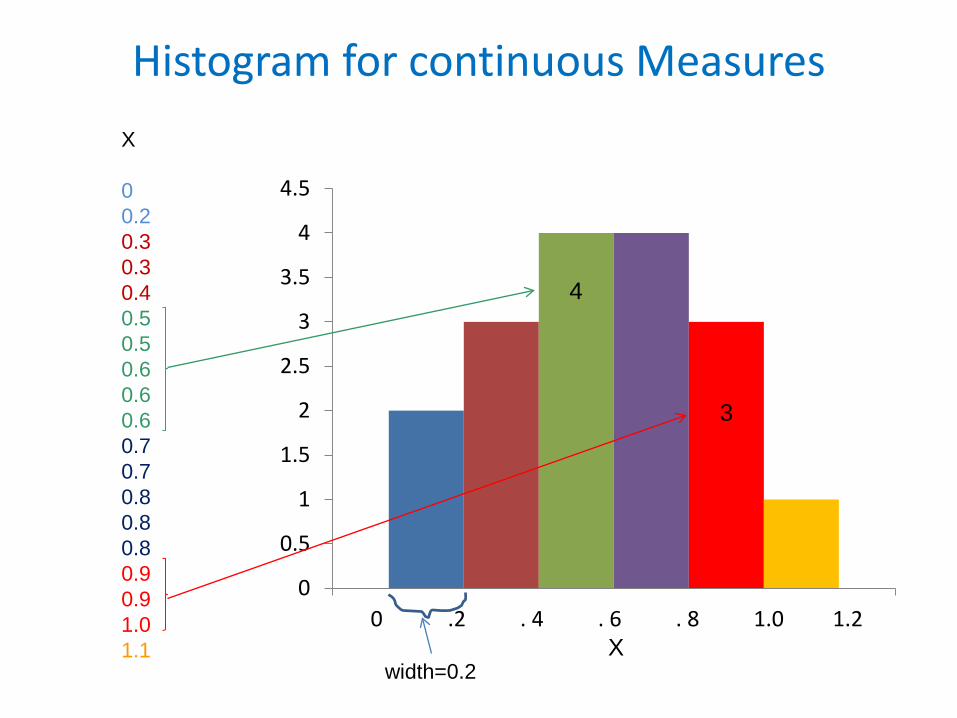
Histogram for continuous Measures

0

0.5

1

1.5

2

2.5

3

3.5

4

4.5

0 .2 . 4 . 6 . 8 1.0 1.2

X

00.20.30.30.40.50.50.60.60.60.70.70.80.80.80.90.91.01.1 X

width=0.2

4

3

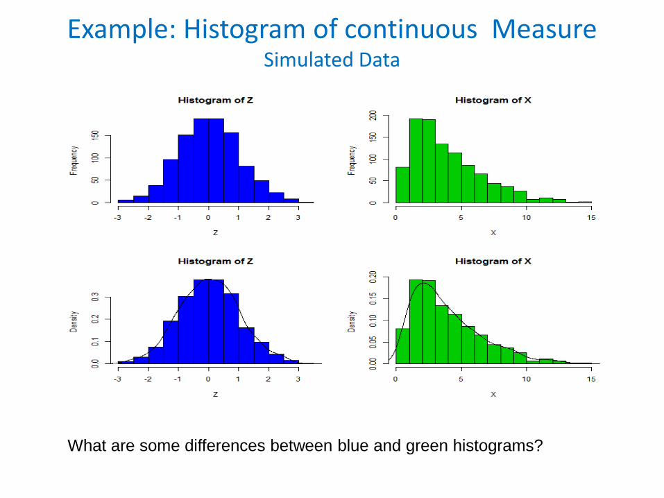
Example: Histogram of continuous MeasureSimulated Data

What are some differences between blue and green histograms?

Boxplots

• What is a boxplot– A box plot or boxplot (box-and-whisker plot) is a graphical toolfor conveying information on location, variation, and symmetry of the data. – It is also used for detecting and illustrating location and variation

differences between two or more groups of data (side-by-side boxplot)

• Why it is useful?It is an efficient visual tool to summarize the main characteristics of the data: Mean/median, quintiles, spread, symmetry and outliers.

Boxplot

*If the data are not normal the length of the whisker is up to the min/max value

Side-by-Side Boxplot Examples Using R(Simulated Data)

– In the second panel the larger the n the wider the box

– Which one has largest median? Smallest IQR?






Normal Distribution• Normal distribution is the most used distribution (and a building

block) in Statistics. It is used to describe and summarize real life data, and also to perform statistical testing

• If X is normally distributed we write:

𝑋𝑋~ 𝑁𝑁(𝜇𝜇,𝜎𝜎2)

– “~” stands for ‘is distributed as’– μ is the mean parameter: μ=∫ 𝑥𝑥𝑓𝑓 𝑥𝑥 𝑑𝑑𝑥𝑥– σ2 is the variance parameter: σ2=∫ 𝑥𝑥 − μ 2𝑓𝑓 𝑥𝑥 𝑑𝑑𝑥𝑥– σ is standard deviation (SD)

• Pdf of X is:

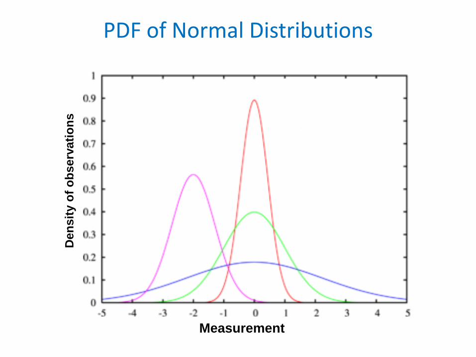
PDF of Normal DistributionsD

ensi

ty o

f obs

erva

tions

Measurement

http://en.wikipedia.org/wiki/Image:Normal_distribution_pdf.png


Does the Mean (μ) Alone Define the Distribution?

A

B

C

Den

sity

of o

bser

vatio

ns

Measurement

D



Standard Deviation (σ)

A

B

C

Den

sity

of o

bser

vatio

ns

Measurement

D

68% of data are between the solid bars which are one standard deviation away from the meanσ



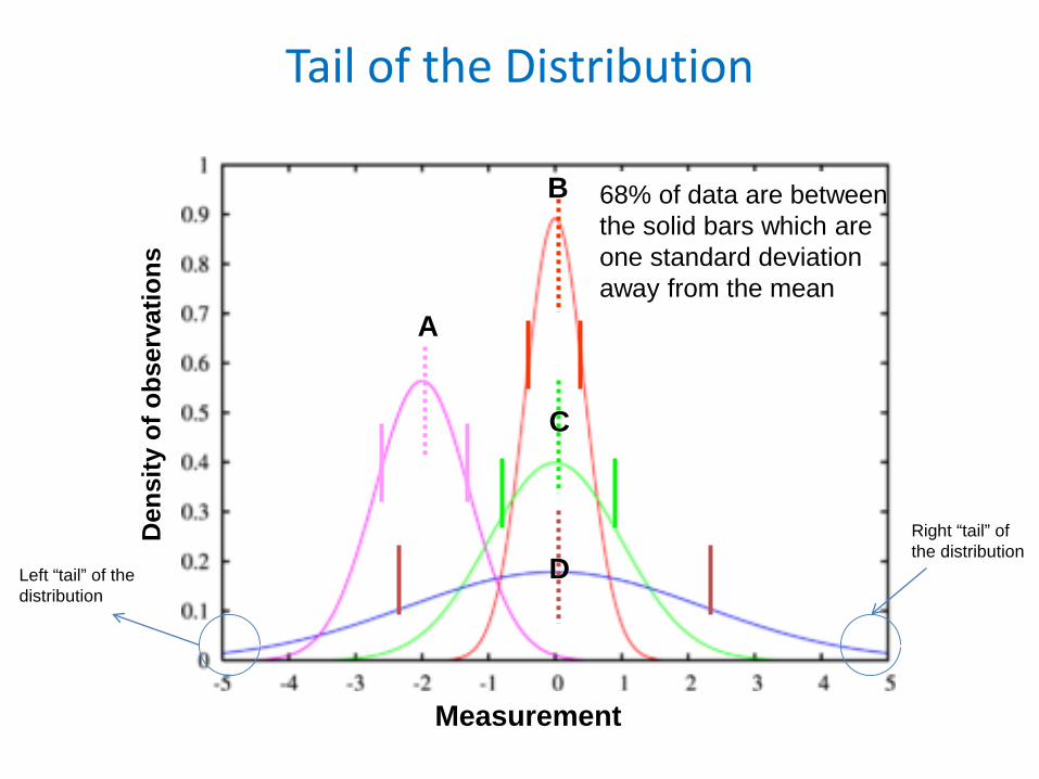
Tail of the Distribution

A

B

C

Den

sity

of o

bser

vatio

ns

Measurement

D

68% of data are between the solid bars which are one standard deviation away from the mean

Right “tail” of the distribution

Left “tail” of the distribution



Characteristics of Normal Distribution

• It is a symmetrical bell-shaped curve– Most frequently occurring points around µ (mean/median)– Points of inflection at µ - σ (standard deviation) and µ + σ– 68/95/99 Rule 68% of the data are within µ - σ and µ + σ

P(µ - σ < X < µ + σ) ≈ .68 95% of the data are within µ - 2σ and µ + 2σ

P(µ - 1.96σ < X < µ + 1.96σ) = .95 99% of the data are within µ - 3σ and µ + 3σ

P(µ - 3σ < X < µ + 3σ)≈.99

– Symmetric to the mean Skewness=0 (Left and right “tail” of the distribution are the same)

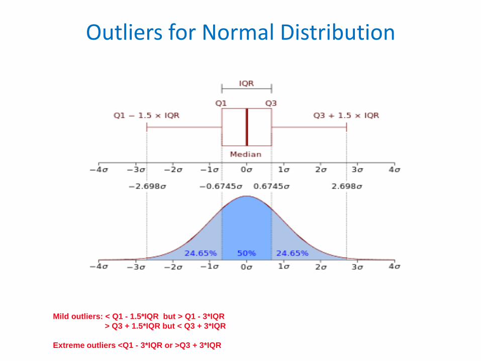
Outliers for Normal Distribution

Mild outliers: < Q1 - 1.5*IQR but > Q1 - 3*IQR> Q3 + 1.5*IQR but < Q3 + 3*IQR

Extreme outliers <Q1 - 3*IQR or >Q3 + 3*IQR

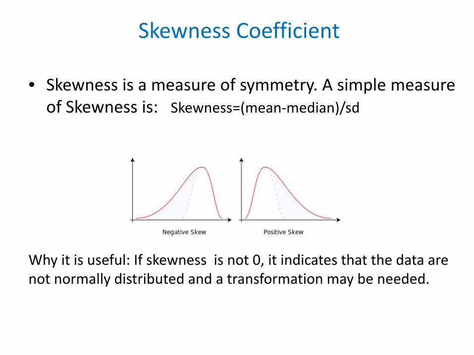
Skewness Coefficient

• Skewness is a measure of symmetry. A simple measure of Skewness is: Skewness=(mean-median)/sd

Why it is useful: If skewness is not 0, it indicates that the data are not normally distributed and a transformation may be needed.

Physiological Distributions(Data from TROPHY Study*)

*Feasibility of treating prehypertension with an angiotensin-receptor blocker. New England Journal of Medicine. 2006; 354:1685-97.

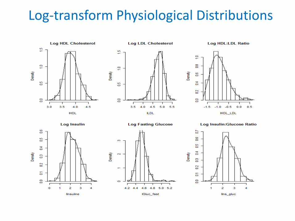
Log-transform Physiological Distributions

Which of These Samples Might Have a Normal Distribution?

A. Height of 50 males in graduate school at U of M in February 2016 Yes.

B. Household income of 10,000 randomly chosen people in the USx No. Skeweness > 0 due to few high earners can stretch the tail to the right.

Testing for Normality

• Plot to “test” for normality– Histograms: Bell shape, symmetry– Boxplot: Symmetry, outliers– Q-Q plot (Quantile-Quantile Plot)

The simplest visual test of normality is the ‘q-q plot’. This plots the quantiles of the observed data against the quantiles from a normal distribution.

If the data are normally distributed then the q-q plot will follow a straight line. Departures from normality show up as various sorts of non-linearity (e.g. S-shapes or banana shapes).

• Shapiro-Wilks test– Formal statistical test for normality

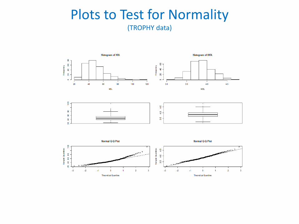
Plots to Test for Normality(TROPHY data)

Shapiro Wilks for Normality

• Shapiro Wilks test is used to formally test for normality In R: shapiro.test(HDL)

shapiro.test(lHDL)

Shapiro-Wilk normality testdata: HDL W = 0.9305, p-value = 1.394e-09

data: lHDLW = 0.9926, p-value = 0.2322

• Conclusion:

If p-value < .05, then reject the hypothesis that data are normal

Shapiro Wilks for Normality

• Shapiro Wilks test is used to formally test for normality In R: shapiro.test(HDL)

shapiro.test(lHDL)

Shapiro-Wilk normality testdata: HDL W = 0.9305, p-value = 1.394e-09 HDL is not normal

data: lHDLW = 0.9926, p-value = 0.2322 No evidence that Log-HDL is not normal

• Conclusion:

If p-value < .05, then reject the hypothesis that data are normal

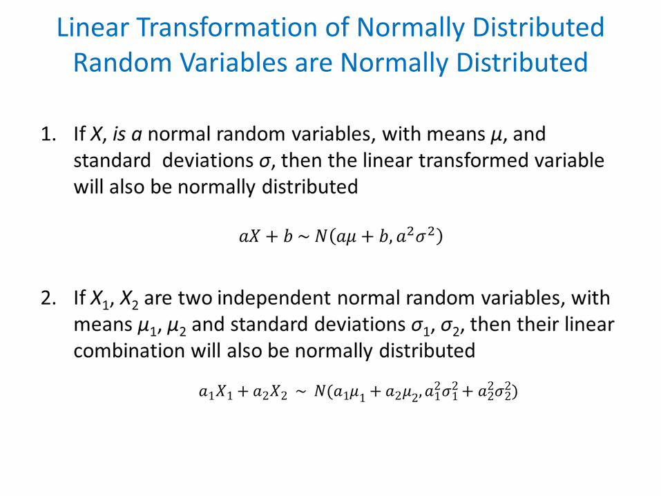
Linear Transformation of Normally Distributed Random Variables are Normally Distributed

Central Limit Theorem (CLT)

• If, x1,x2,….,xn is a sequence of independent identically distributed random variables, each having mean 𝜇𝜇 and variance 𝜎𝜎2, then the CLT states that as the size (n) of the sample gets large, the distribution of

�̅�𝑥, (or ∑𝑖𝑖 𝑥𝑥𝑖𝑖 ) becomes normally distributed with E(Y)= 𝜇𝜇, Var(Y)=𝜎𝜎𝑛𝑛

2.

�̅�𝑥→𝑑𝑑𝑁𝑁(𝜇𝜇, 𝜎𝜎

𝑛𝑛

2) or ∑𝑖𝑖 𝑥𝑥𝑖𝑖 = →

𝑑𝑑𝑁𝑁(𝑛𝑛𝜇𝜇,𝑛𝑛𝜎𝜎2)

• Why is CLT important: If n is fairly large (n > 30), then following CLT one can implement statistical tests related to the �̅�𝑥 (or ∑𝑖𝑖 𝑥𝑥𝑖𝑖 ) that are based on normal distributed theory even if xi are not normally distributed.

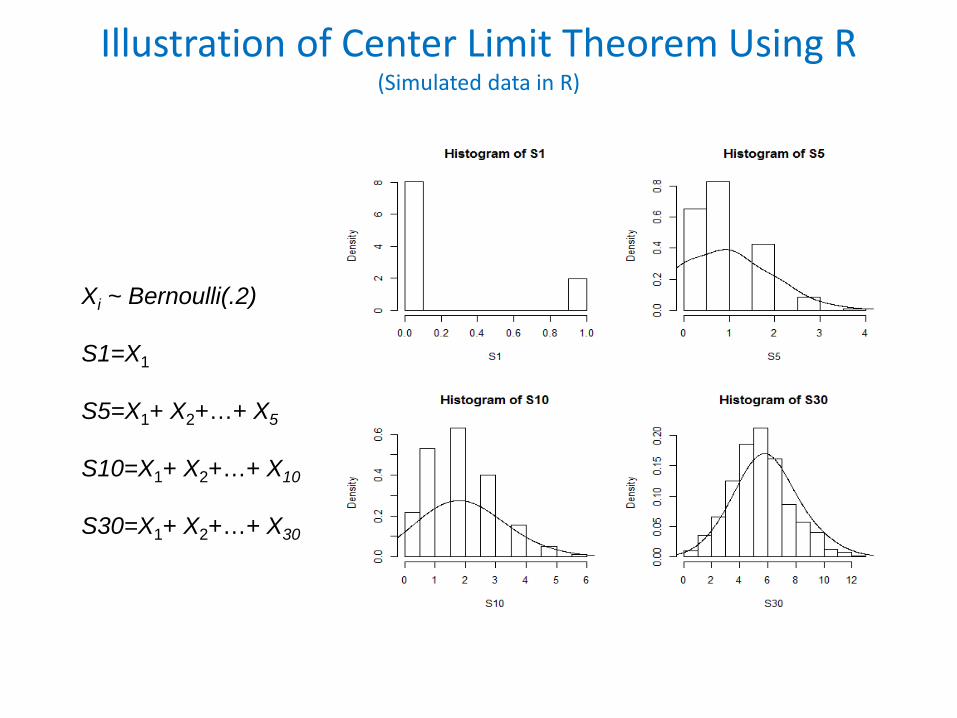
Illustration of Center Limit Theorem Using R(Simulated data in R)

Xi ~ Bernoulli(.2)

S1=X1

S5=X1+ X2+…+ X5

S10=X1+ X2+…+ X10

S30=X1+ X2+…+ X30

Application of CLT: 95% Confidence Intervals

• From CLT: �̅�𝑥→𝑑𝑑𝑁𝑁(𝜇𝜇, 𝜎𝜎

𝑛𝑛2

) then (from 68/95/99 rule)

Pr[𝜇𝜇 -1.96*σ/ 𝑛𝑛< 𝑥𝑥 < 𝜇𝜇 + 1.96∗σ/ 𝑛𝑛] = 0.95or

Pr[𝑥𝑥-1.96*s𝑒𝑒(𝑥𝑥) < μ < 𝑥𝑥 + 1.96 ∗ 𝑠𝑠𝑒𝑒(𝑥𝑥)] = 0.95where s𝑒𝑒 𝑥𝑥 is an estimate for �σ 𝑛𝑛.

• [𝑥𝑥 −1.96*s𝑒𝑒 𝑥𝑥 , 𝑥𝑥 + 1.96 ∗ 𝑠𝑠𝑒𝑒(𝑥𝑥)] is referred as the 95%Confidebce Interval (95%CI) for μ

• More general: If �β is an estimate for β then: [�β −1.96*s𝑒𝑒 �β , �β + 1.96 ∗ 𝑠𝑠𝑒𝑒(�β)] is the 95%CI for β

• Why are Confidence Intervals (CI) important?

CI are Important When Making Inferences About a Population Based on a Sample

• Statistical Inference: Drawing conclusion based on data. Estimating the characteristics or properties of a population derived from the analysis of a sample drawn from it.– What do 𝑥𝑥 and s tell us about μ and σ?

How Close are Sample Values to Population Values?

Confidence intervals are used to indicate the reliability of an estimate






T-distribution

Illustration of T-distribution (Simulated Data in R)

Statistical Tests using T-distribution

• T-distribution and t-test (or Student’s t-test) – One sample t-test, – Two sample t-test – Paired t-test

χ2 distribution

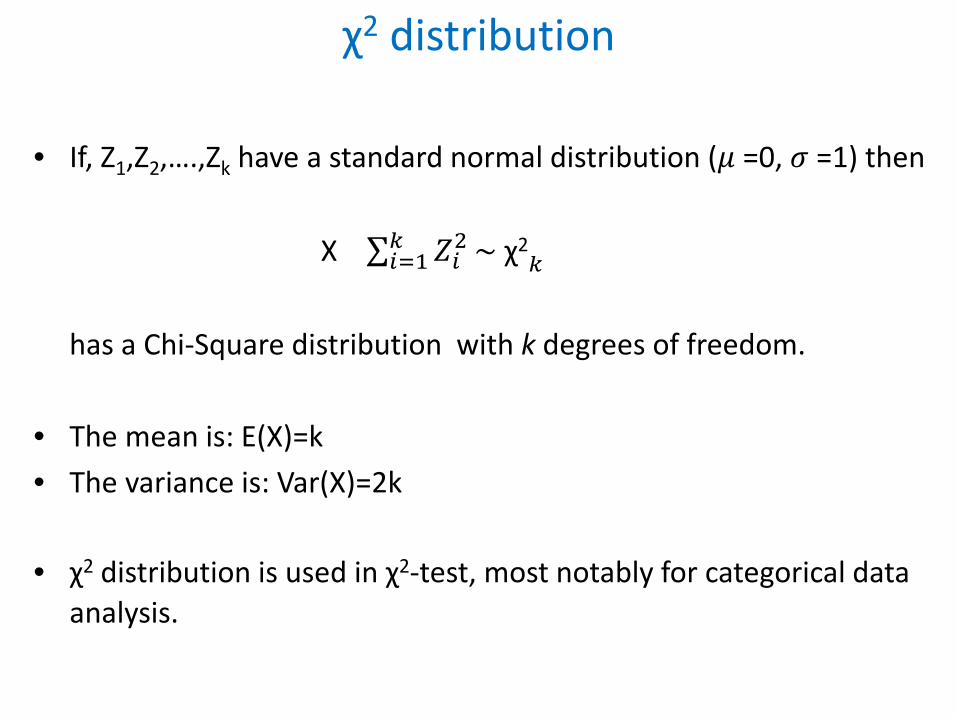
• If, Z1,Z2,….,Zk have a standard normal distribution (𝜇𝜇 =0, 𝜎𝜎 =1) then

X=∑𝑖𝑖=1𝑘𝑘 𝑍𝑍𝑖𝑖2 ~ χ2𝑘𝑘

has a Chi-Square distribution with k degrees of freedom.

• The mean is: E(X)=k• The variance is: Var(X)=2k

• χ2 distribution is used in χ2-test, most notably for categorical data analysis.

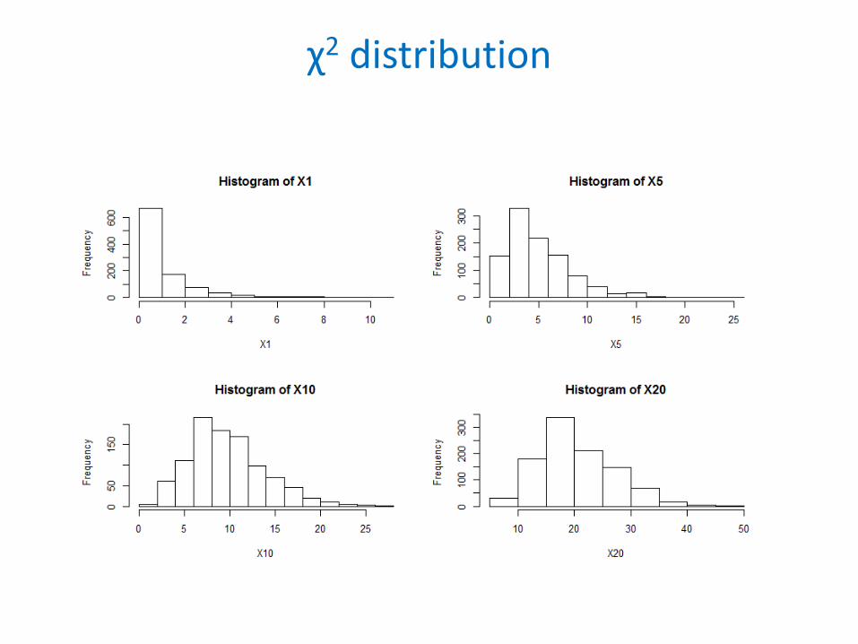
χ2 distribution

F distribution

• If χ𝑛𝑛2and χ𝑚𝑚

2 are independent following Chi-Square distribution with n and m degrees of freedom, then their scaled ratio has an F distribution with (n, m) degrees of freedom:

F𝒏𝒏,𝒎𝒎=⁄χ𝑛𝑛2 𝑛𝑛⁄χ𝑚𝑚2 𝑚𝑚

• F distribution is used in the F-test, most notably regression analysis or the analysis of variance

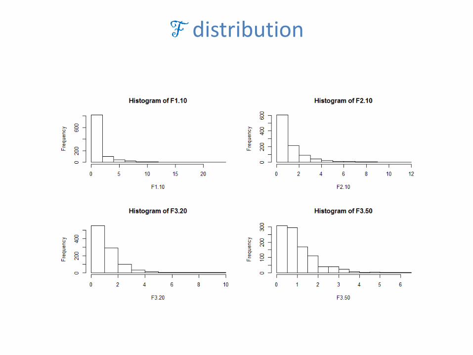
F distribution

Few Summary Points

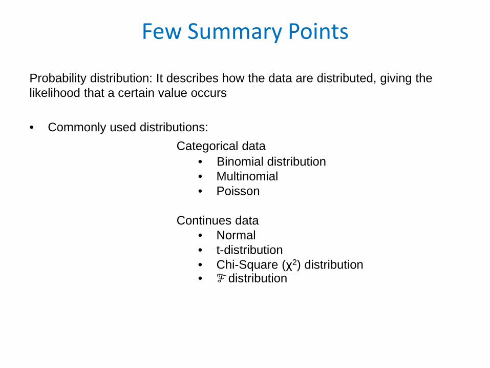
Probability distribution: It describes how the data are distributed, giving the likelihood that a certain value occurs

• Commonly used distributions:Categorical data

• Binomial distribution • Multinomial • Poisson

Continues data • Normal• t-distribution• Chi-Square (χ2) distribution • F distribution

Few Summary Points

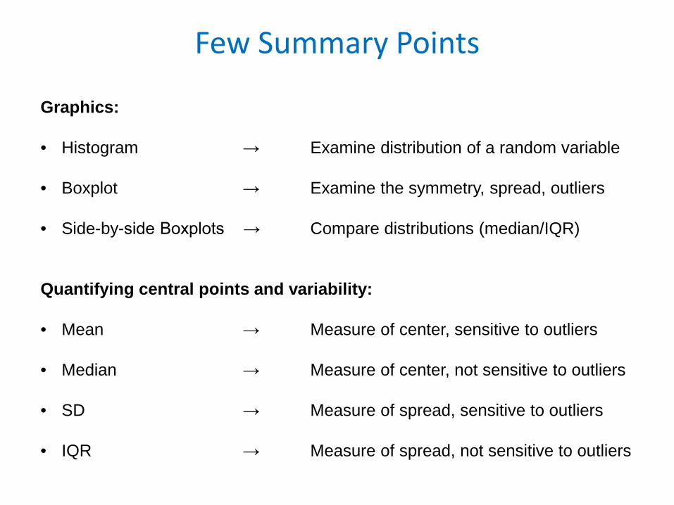
Graphics:

• Histogram → Examine distribution of a random variable

• Boxplot → Examine the symmetry, spread, outliers

• Side-by-side Boxplots → Compare distributions (median/IQR)

Quantifying central points and variability:

• Mean → Measure of center, sensitive to outliers

• Median → Measure of center, not sensitive to outliers

• SD → Measure of spread, sensitive to outliers

• IQR → Measure of spread, not sensitive to outliers

Few Summary Points

Test for Normality:

• Histogram → Symmetric bell-shape

• Boxplot → Symmetric, no outliers

• Q-Q Plot → Visual comparison with a normal distribution

• Shapiro-Wilks test → Statistical test for normality

Documents

Module 2: Introduction to Statistics