Models of Categorization

vi. R., lcture Juted nand

983). lrain,

:::ate-1and 273-

Catrain,

lows !il & itian

tiga-

nahal-

lroern )),

CHAPTER 9

Models of Categorization

John K. Kruschke

In: Ron Sun (Ed.), 2008. The Cambridge Handbook of

Computational Psychology. New York: Cambridge University Press.

1. Introduction

This chapter surveys a variety of formal models of categorization, with emphasis on exemplar models. The chapter reviews exemplar models' similarity functions, learning algorithms, mechanisms for exemplar recruitment, formalizations of response probability, and response dynamics. The intended audience of this chapter is students and researchers who are beginning the daunting task of digesting the literature regarding formal models of categorization. There are numerous variations for formalizing the component processes in exemplar models of categorization, and one of the contributions of the chapter is a direct comparison of component functions across models. For example, the similarity functions of several different models are expressed in a shared notational format, and formulas for the special case of present/absent features are derived, which permits direct comparison of their behaviors. No previous review cuts across models this way, also including comparisons of learning, exemplar recruitment, and so forth.

By decomposing the models and displaying corresponding components side by side, the chapter intends to reveal some of the issues that motivate model builders, and to identify some of the unresolved issues for future investigators. Along the way, a few promising but undeveloped ideas are pointed out, such as an identity-sensitive similarity function (Kruschke, 1993), a new gradient-descent learning rule for the Supervised and Unsupervised Stratified Adaptive Incremental Network (SUSTAIN) model (Love, Medin, & Gureckis, 2004), an attentionally modulated exemplar recruitment mechanism (Kruschke, 2003b), a proposal for cascaded activation in Attentional Learning Covering map (ALCOVE; Kruschke, 1992), among others.

Whereas this chapter is specifically intended to survey exemplar model formalisms, it avoids discussions of the various empirical effects explained or unexplained by each model variation. A survey of empirical phenomena can be found in the highly readable book by Murphy (2002) . A chapter by Goldstone and Kersten (2003) describes the various roles of categorization in

KRUSCHKE

cognition. Another chapter by Kruschke (2005) surveys models of categorization with special emphasis on the role of selective attention and attentionallearning. Previous reviews by Estes (1993, 1994) emphasize particular exemplar models and associated empirical results through the early 1990s.

1.1. Everyday Categorization

Everyone does categorization. For example, if you were in an office, and your companion pointed to the piece of furniture by the desk and asked, "What's that?" you would easily reply, "It's a chair." Such facility in categorization is not to be taken sitting down: There are hundreds of different styles of chairs, many of them novel, seen from thousands of different angles, yet all can be effortlessly categorized as chair. Whereas people include many items in the category chair, they also exclude similar items that are categorized instead as a park bench or a car seat. Putting those examples behind us, we conclude, a posteriori, that categorization is a complex process.

Categorization is not just an armchair amusement. It has consequences with costs or benefits. If you mistakenly categorize a dog as a chair and try sitting on it, the category of teeth might suddenly leap to mind. You might think it is ridiculous to confuse a dog with a chair, but there are children's chairs manufactured to resemble dogs. Moreover, categorizing a dog as a dog is not always easy; a Labrador is doggier than a Pekinese. A humorous consequence of category atypicality was revealed in a 1933 cartoon by Rea Gardner in the New Yorker Magazine: A rotund wealthy lady enters a posh restaurant clutching her tiny lap dog, to which the snooty maitre d' remarks, ''I'm sorry, Madam, but if that's a dog, it's not allowed." For a more thorough review of the many uses and consequences of categorization, see the chapter by Goldstone and Kersten (2003).

1.2. Categorization in the Laboratory

Models of categorization are usually designed to address data from laboratory ex-

periments, so "categorization" might be best defined as the class of behavioral data generated by experiments that ostensibly study categorization. Perhaps the iconic categorization experiment is one that presents a stimulus to an observer and asks him or her to select a classification label for the stimulus. In some experiments, corrective feedback is then supplied.

There are many kinds of procedures and measurements in categorization experiments, which can assay many different aspects of behavior. One such measure is the proportion of times each category label is chosen when a stimulus is presented repeatedly on different occasions. Experimenters can also measure confidence ratings, response times, typicality ratings, eye gaze, recognition accuracy or rating, and so forth. Those dependent variables can be assessed as a function of many different independent variables. For example, behavior can be tracked as a function of the number of stimulus exposures, whereby the experimenter can assess learning, priming, habituation, and so forth. Experimenters can also manipulate category structure, that is, how the stimuli from different categories are situated relative to each other. (For example, the categories "stars in Orion" and "stars in the Big Dipper" are fairly easy to distinguish because their structures put them in distinct regions of the sky. But the categories "stars closer than 50 light years" and "stars farther than 50 light years" are more difficult to distinguish because stars from those categories are scattered in overlapping regions of the sky.) The variety of independent variables is bounded only by the experimenter's imagination. A very accessible review of the empiricalliterature has been presented by Murphy (2002).

1.3. Informal and Formal Models

It is the constellation of categorization phenomena that theorists want to explain. Informal theories provide some insights into the possible shapes behind that constellation. For instance, one may informally hypothesize that a bird is defined by necessary and sufficient features: A bird is something

~ best ener;tudy tego:lts a r her ;tim~ed-

.ures )erit ase is , la-1ted )erirateye :l so asin

lior ber erituIlso ow 5itlIe, in

ish 1Ct ::lrs ler is. es he is ~i-

or-

'-

1-

o [ -

y g

MODELS OF CATEGORIZATION

that flies, sings, and has feathers. By that definition, however, a bird can be an opera diva wearing a feather boa in an airplane. So, instead, one might informally hypothesize that a bird is defined by similarity to a prototype: A bird is something like a robin, which is an often-seen bird for North Americans.

Informal theories are a very useful first step in creating explanations of complex behaviors. Unfortunately, informal theories rarely make precise predictions and are often difficult to distinguish empirically. Sometimes, it is only intuition that generates predictions from an informal theory, so different theorists can make different predictions from the same informal theory.

All branches of science progress from informal theory to formal model. If all that Isaac Newton did was propose informally that there is a mysterious force that acts on apples and the moon in the same way, it is unlikely that his theory would be remembered today. It was the precision and veracity of his formal model of gravity that made his idea famous. Whereas Newton invented a formal model of how apples and moons interact among themselves, cognitive scientists have been inventing formal theories of how apples and moons are mentally categorized by observers. Just as there are many possible aspects of objects that could be formally speCified in a model of gravitational behavior, there are many aspects of mental processing that could be formally specified in a model of categorical behavior.

1.4. Types of R epresentation and Process

Any model must assume that the stimulus is represented by some formal description. I This input representation could be de-

I This representational assumption for a model does not necessarily imply that the mind makes a formal representation of the stimulus. Only the formal model requires a formal description. This is exactly analogous to formal models of motion: Newton's formal model uses representations of mass and distance to determine force and acceleration, but the objects themselves do not necessarily measure their masses and distances and then compute their force and acceleration. The representations in the model help us understand the behavior, but those repre-

rived from multidimensional scaling (e.g., Kruskal, 1964; Shepard, 1962). For example, an animal might be represented by its precise coordinates in a psychological space that includes dimensions of size, length of hair/fur, and ferocity. Other methods for deriving a stimulus representation include feature extraction from additive clustering or factor analysis. Any model must also assume a formal representation of the cognizer's response. In the case when the cognizer is asked to produce a category label for a presented stimulus, the formal representation of the response could be a simple 1/0 coding for the presence/absence of each possible category label.

Some key differences among models are the representations and transformations that link the input and response representations. These intermediate representations and transformations are supposed to describe mental processes. 2 In general, a model of categorization specifies three things: (1) the content and format of the internal categorical knowledge representation, (2) the process of matching a to-be-classified stimulus to that knowledge, and (3) a process of selecting a category (or other response) based on the results of the matching process.

It can be useful to categorize models of categorization according to the content and format of their internal knowledge. Essentially, this content and format describe the type of representation that models use to mediate the mapping from input to output . The usual five types of representation are exemplars, prototypes, rules, boundaries, and theories. Many models of categorization are explicitly designed to be a clear case of one of those representational types, and some models are explicitly designed to be hybrids of those types, whereas yet other models are not easily classified as one of the five.

sentations need not be reified in the behavior being modeled.

2 Just as input and output representations are in the model but not necessarily in the world, an intermediate transformation and representation in the model need not be reified in the mind being modeled.

KRUSCHKE

1.4.1. EXEMPLAR MODELS

The canonical exemplar model simply stores every (distinct) occurrence of a stimulus and its category label. To classify a stimulus, the model determines the similarity of the stimulus to all the known exemplars, aggregates the similarities, and then decides the categorization of the stimulus. Exemplar models are the primary focus of this chapter and will be discussed extensively later. The other types of models are only briefly described to establish a context for exemplar models .

1.4.2. PROTOTYPE MODELS

A prototype model operates analogously to an exemplar model, but instead of storing information about every instance, the model only stores a summary representation of the many instances in a category. This representative stimulus could be a central tendency that expresses an average of the category. This average need not be the same as any actually experienced instance. The representative prototype could instead be a modal stimulus defined either as the most frequent instance or as a derived stimulus that is a combination of all the most frequent features . In the latter case, this modal stimulus need not be the same as any actually experienced instance. Finally, the prototype could instead be an "ideal" exemplar or caricature that indicates not only the content of the items in the category but also emphasizes those features that distinguish the category from others. This ideal need not be actually attained by any real instance of the category.

In "pure" prototype models, the models take a stimulus as input, compute its similarity to various explicitly speCified prototypes, and then generate categorical response tendencies. A famous early application of a prototype model to human classification of schematic faces was conducted by Reed (1972). Anyone-layer feed-forward connectionist model can be construed as a prototype model; an example is the componentcue model of Gluck and Bower (1988), in which a category is defined by a vector of weighted connections from features. (For

a discussion of connectionist models, see Chapter 2 in this volume.)

Pure prototype models have a single explicit prototype per category. It is possible instead to represent a category with multiple prototypes, especially if the category is multimodal or has "jagged" boundaries with adjacent categories. Taken to the limit, this multiple-prototype approach can assign one prototype per instance, so it becomes an exemplar model. Some examples of models that recruit multiple prototypes during learning of labeled categories will be discussed later, but there are also models that recruit multiple prototypes while trying to learn clusterings among unlabeled items (e.g., Carpenter & Grossberg, 1987; Rumelhart & Zipser, 1985) .

In another form of prototype model, the prototypes for the categories are implicit and dynamic (and in fact, it might be debatable to assert that these models "have" prototypes at all). An example of this sort of model is a recurrent connectionist network. When a few nodes in the network are clamped "on/' activation spreads via weighted connections to other nodes. Some other nodes will be stably activated, whereas other nodes will be suppressed. If each node represents a feature, then the collection of co-activated nodes can be interpreted as having filled in the typical features of the category to which the initially clamped-on features belonged. Models that implement this approach include the "brain state in a box" model of Anderson et al. (1977) and the constraint-satisfaction network of Rumelhart et al. (1986).

1.4· 3· RULE MODELS Another type of model that specifies a category by a summary of its content is a rule model. A rule is a list of necessary and sufficient features for category membership. For example, a bachelor is anything that is human, male, unmarried, and eligible. (Notice that the features themselves are categories.) Examples of rule models include the hypothesis-testing approach of Levine (1975) and the RULEX model of Nosofsky et al. (Nosofsky & Palmeri, 1998j Nosofsky, Palmeri, & McKinley, 1994).

{

Ie 1--y ~s

t, ,-

~s

~s

e Is g lS

1-

e d e ·s

:l n :i

s s s :l 1

1


1.4+ BOUNDARY MODELS

Unlike the previously described types of models, a boundary model does not explicitly specify the content of a category but instead specifies the boundaries between categories. For example, one might define a skyscraper as any building that is at least twenty stories tall. The value, twenty stories, is the boundary between skyscraper and non-skyscraper. Sometimes, boundary models are also referred to as rule models, because the boundary is a specific condition for category membership just like necessary and sufficient features are a specific condition . The usage here emphasizes that rules specify interior content, whereas boundaries specify edges between. The best developed boundary models have been expounded in a series of publications by Ashby and collaborators (e.g ., Ashby & Gott, 1988; Ashby & Maddox, 1992)

1.4-5- CONTE T/BOUNDARY DUALITY

AND ON-THE-FLY EQUIVALENCE

In some cases, it is only a matter of emphasis to think of a model as specifying content or boundary, because there may be ways to convert a content model to an equivalent boundary model and vice versa. For example, suppose two categories are represented by one prototype for each category, and the categorization is made by classifying a stimulus as whichever prototype is closer. From this it can be easily inferred that the model makes a linear boundary between the two categories, and an equivalent model states that the stimulus is classified by whichever side of the linear boundary it falls on.

lt might be possible in principle to convert any content model to an equivalent boundary model and vice versa, but that does not mean that the two types of models are equally useful. Especially when category structure is complex, when there are many categories involved, and when new categories might be created, it is probably easier to describe a category by content than by boundary. For example, if new category members are observed that are somewhat different from previously learned instances, it is easy to simply add the new items to

memory, but potentially difficult to add explicit "dents" in all the category boundaries between that category and many others. The actual difficulty depends on the particular formalization of boundaries, so this intuitive argument must be considered with caution.

There is another way in which a pure exemplar model encompasses the others. If a cognizer has perfect memory of all instances encountered, then the cognizer could, in principle, generate prototypes, rules, or theories at any moment, on the fly, and use those derived representations to categorize stimuli. Although this process is possible, presumably it would generate long response latencies compared with a process that has those representations immediately available because of previously deriving them during learning.

1.4.6. THEORY MODELS

The fifth approach to models of categorization is the "theory theory." This approach asserts that people have theories about the world, and people use those theories to categorize things. This approach can explain a variety of complex phenomena that are difficult for simpler models to address. The primary statement of this approach was written by Murphy and Medin (l985), and more recent reviews have been writtten by Murphy (1993,2002). Theory theories have had limited formalizations, however, in part because it can be difficult to formally specify all the details of a complex knowledge structure. Some recent models that include formalizations of previous knowledge, if not full-blown theories, are those by Heit and Bott (2000); Heit, Briggs, and Bott (2004) and Rehder (2003a, 2003b).

1.4-7. HYBRID MODELS

The various representations and processes described in previous sections have different properties, and it may turn out to be the case that no single representation captures all of human behavior. It is plausible that the breadth of human behavior is best explained by a model that uses multiple representations. The challenge to the theorist then goes beyond specifying the details of anyone

KRUSCHKE

representational type. The theorist must also specify exactly how the different representations interact and the circumstances under which each subsystem is selected for action or learning. Only a few combinations of representation have been explored.

Busemeyer, Dewey, and Medin (1984) combined prototype and exemplar models and found no consistent benefit of including prototypes. A model proposed by Smith and Minda (2000) combined prototypes with punctate exemplars, in which only exact matches to the exemplars have an influence; but Nosofsky (2000) showed that this particular hybrid model has serious shortcomings.

Other models have combined rules or boundaries with exemplars or multiple prototypes. For example, the COVIS model (Ashby et aL, 1998; Ashby & Maddox, 2005) includes two subsystems, an explicit verbal subsystem that learns boundaries aligned with stimulus dimensions and an implicit system that learns to map exemplars or regions of stimulus space to responses. As another example, a "mixture of experts" approach (Erickson & Kruschke, 1998, 2002; Kalish, Lewandowsky, & Kruschke, 2004; Kruschke, 2001a; Kruschke & Erickson, 1994; Yang & Lewandowsky, 2004) combines modules that learn boundaries and modules that learn exemplar mappings. The mixture-of-expert approach also incorporates a gating system that learns to allocate attention to the various modules.

1.5. Learning of Categories

A model of categorization can specify a mapping from input to output without specifying how that mapping was learned. Theories of learning make additional assumptions about how internal representations change with exposure to stimuli. Different types of representation may require different types of learning. This section merely mentions some of the various possibilities for learning algorithms. Examples of each are described in Section 2.

Perhaps the simplest learning mechanism is a tally of how many times a particu-

lar feature co-occurs with a category labeL Somewhat more general are simple Hebbian learning algorithms that increment a connection weight by a constant amount whenever the two nodes at the ends of that connection are co-activated. More sophisticated Hebbian algorithms adjust the size of the increment so that the magnitude of the weight is limited. Notice that in these schemes the weights are adjusted independently of how well the system is performing its categorization.

Alternatively, learning could be driven by categorization performance, not by mere cooccurrence of stimuli. The model can compare its predicted categorization with the actual category and, from the discrepancy, adjust its internal states to reduce the error. Thus, error minimization can be one goal for learning. In other approaches to learning, the goal is to adjust the internal representation such that it maximizes economy of description or the amount of information transmitted through the system.

Yet another scheme is learning by Bayesian updating of beliefs regarding alternative hypotheses. In the previous nonBayesian schemes, learning was a matter of adjusting the values of a set of parameters, such as associative weights. By contrast, in a Bayesian framework, there are a large set of hypothetical fixed parameter values, each with a certain degree of belief. Bayesian learning consists of shifting belief away from hypotheses that fail to fit observations, toward hypotheses that better fit the observations.

2. Exemplar Models

The previous section provided a brief informal description of some of the concepts that will be formally expressed in the remainder of the chapter. From here on, the chapter unabashedly employs many mathematical formulas to express ideas.

In recent decades, theories of categorization emphasized rule-based theories (e.g., Bourne, 1966; Bruner, Goodnow, & Austin} 1956), then changed to prototype-based

)-

a

1t

'it

5-

:e )f ;e 1-

.g

y )-

1-

e

y :l

y

f

1

t


theories (e.g., Reed, 1972; Rosch & Mervis, 1975), and then moved to boundary (e.g., Ashby & Gott, 1988) and exemplar theories (e.g., Medin & Schaffer, 1978; Nosofsky, 1986). Although a variety of representations have been formalized, exemplar models have been especially richly explored in recent years, in no small part because they have been shown to fit a wide variety of empirical data. Exemplar models also form a nice display case for illustrating the issues mentioned in the preceding introductory paragraphs.

2.1. Exemplary Exemplar Models

Exemplar models have appeared in domains other than categorization, such as perception, memory, and language (e.g., Edelman & Weinshall, 1991; Hintzman, 1988; Logan, 2002; Regier, 2005). Within the categorization literature, however, a dominant family line of exemplar models centers on the Generalized Context Model (GCM; Nosofsky, 1986). The GCM is a formal generalization of the context model of Medin and Schaffer (1978). In these models, a stimulus is stored in memory as a complete exemplar that includes the full combination of stimulus features . It is not the case that each feature is stored independently of other features. Thus, the "context" for a feature is the other features with which it co-occurs. Exemplar representation allows the models to capture many aspects of human categorization, including the ability to learn nonlinear category distinctions and correlated features, while at the same time producing typicality gradients.

In the context model and GCM, perhaps just as important as exemplar representation is selective attention to features. With selective attention, the same underlying exemplar representation can be used to represent different category structures in which different features are relevant or irrelevant to the categorization. The context model and GCM had no learning mechanism for attention, however. Kruschke (1992) provided such a learning mechanism for attention in the ALCOVE model and at the same time

provided an error-driven learning mechanism for associations between exemplars and categories (unlike the simple frequency counting used in the GCM). Hurwitz (1994) independently developed a similar idea but based on the formalism of the context model, not the GCM. Attentional shifting in ALCOVE was assumed to be gradual over trials, but human attentional shifting is probably much more rapid within trials while retention is gradual across trials. Rapid attention shifts were implemented in the Rapid Attention Shifts 'N' Learning (RASHNL) model of Kruschke and Johansen (1999). The basic formulas for the GCM and ALCOVE are presented next, so that subsequent researchers ' variations of these formulas can be provided.

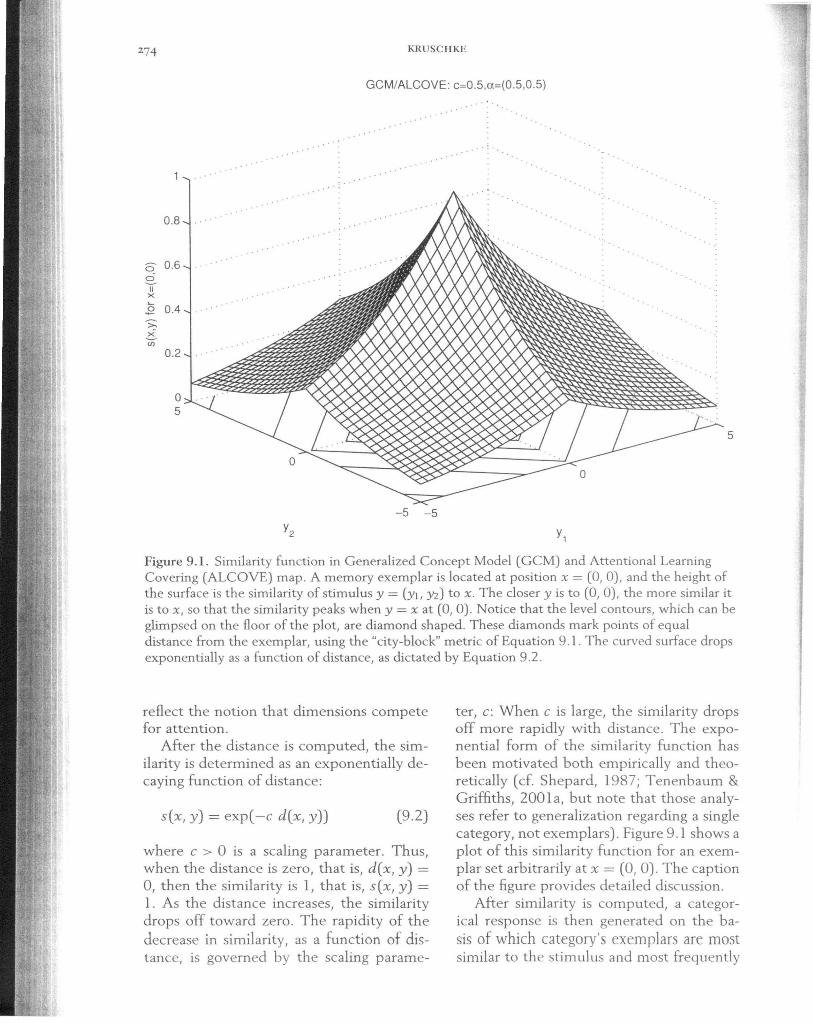
The GCM assumes that stimuli are points in an interval-scaled multidimensional space. For example, a stimulus might have a value of 47 on the dimension of perceived size and a value of 225 on the dimension of perceived hue. Formally, exemplar x has value Xi on dimension i.

The similarity between memory exemplar x and stimulus y is computed in two steps. First, the psychological distance between x and y is computed:

(9 .1)

where (Xi is the attention allocated to dimension i. Equation 9.1 simply says that for each dimension i, the absolute difference between x and y is computed, and then those dimensional differences are added up to determine the overall distance. Each dimension contributes to the total distance only to the extent that it is being attended to; the degree of attention to dimension i is captured by the coefficient (Xi (which is non-negative). Notice that when (Xi gets larger, the difference on dimension i is weighted more heavily in the overall distance function. Equation 9.1 applies when the dimensions are psychologically separable; that is, when they can be selectively attended. In some applications, the attention strengths are assumed to sum to 1.0, to

KRUSCHKE

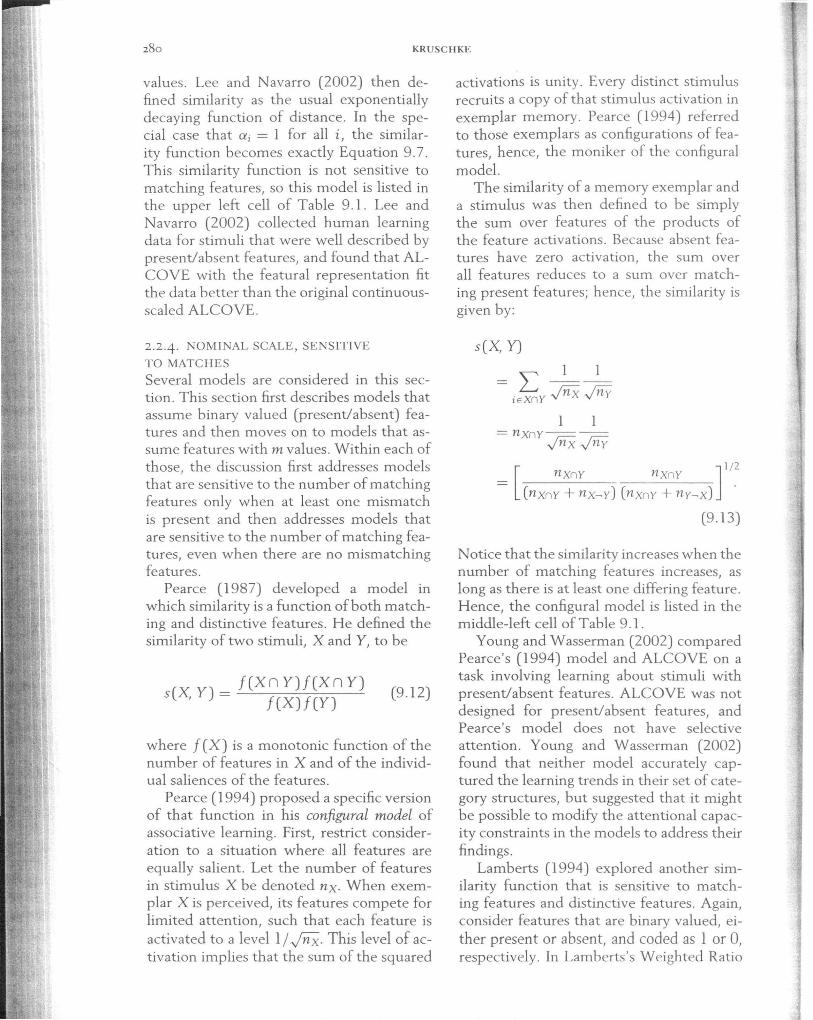
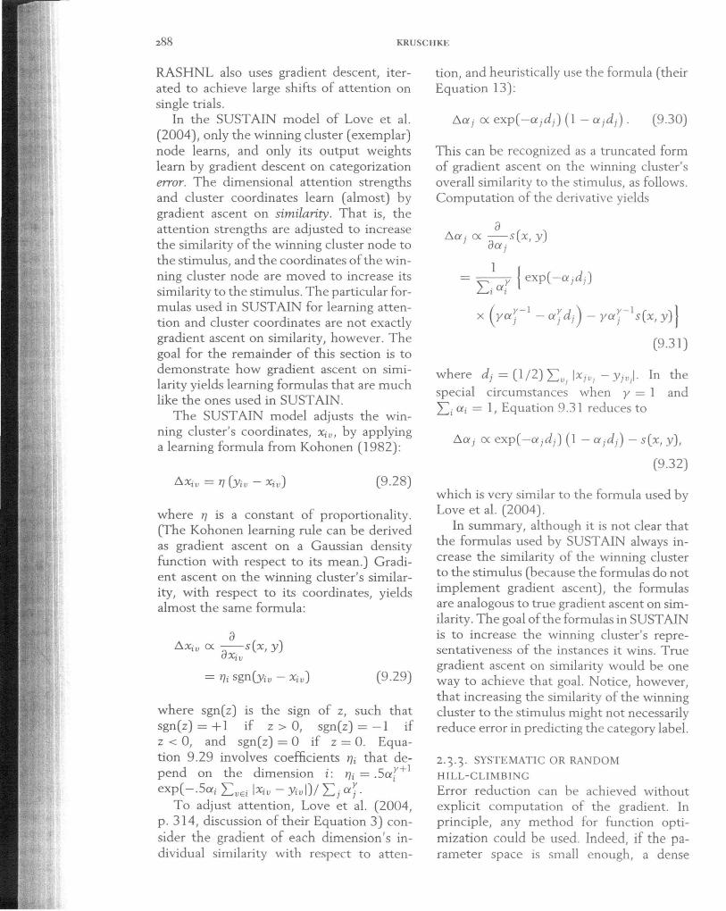
GCM/ALCOVE: c=0.5,o:=(0.5,0.5)

. . ......

. ' . ,, ' .

0.8

0.: 0.6 2-

II x

.2 0.4 >; 2:S (f)

0.2

0 5

5

-5 -5

Y2 Y1

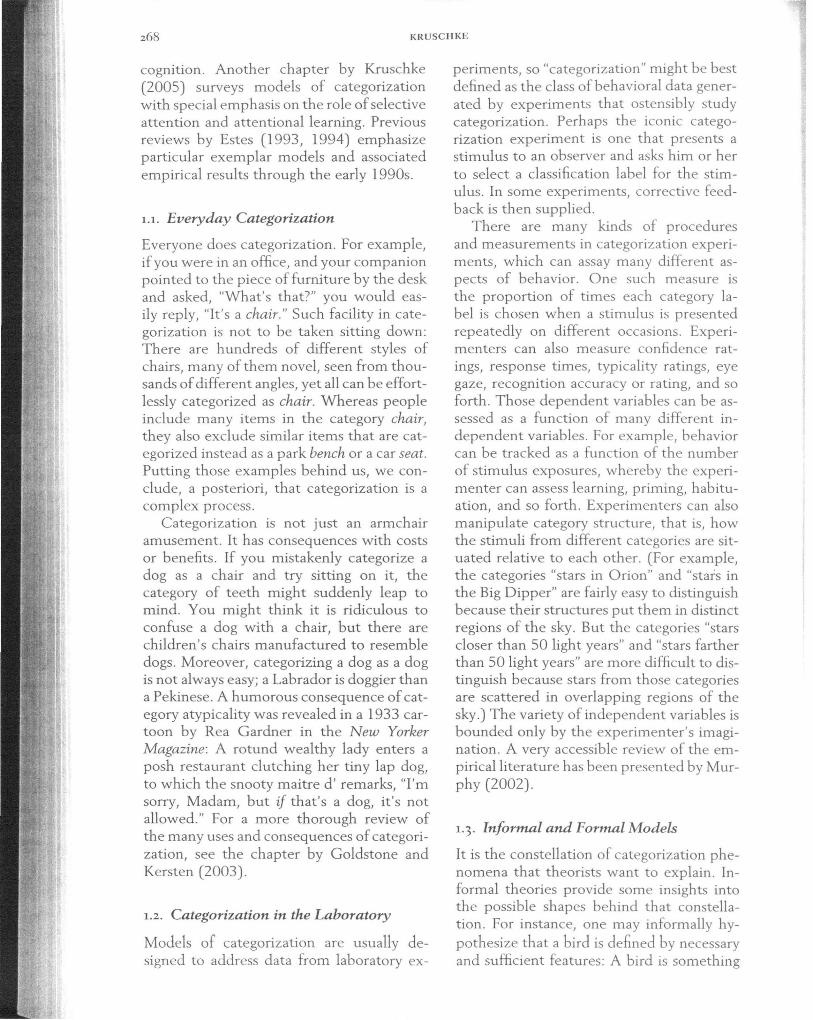
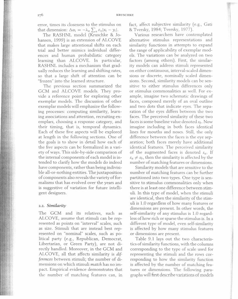
Figure 9 .1. Similarity function in Generalized Concept Model (GCM) and Attentional Learning Covering (ALCOVE) map. A memory exemplar is located at position x = (0, 0), and the height of the surface is the similarity of stimulus y = (YI, Yz) to x. The closer y is to (0, 0), the more similar it is to x, so that the similarity peaks when y = x at (0,0). Notice that the level contours, which can be glimpsed on the floor of the plot, are diamond shaped. These diamonds mark points of equal distance from the exemplar, using the "city-block" metric of Equation 9.1. The curved surface drops exponentially as a function of distance, as dictated by Equation 9.2.

reflect the notion that dimensions compete for attention.

After the distance is computed, the similarity is determined as an exponentially decaying function of distance:

sex, y) = exp( -c d(x, y)) (9.2)

where c > 0 is a scaling parameter. Thus, when the distance is zero, that is, d(x, y) = 0, then the similarity is I, that is, sex, y) = 1. As the distance increases, the similarity drops off toward zero. The rapidity of the decrease in similarity, as a function of distance, is governed by the scaling parame-

ter, c: When c is large, the similarity drops off more rapidly with distance. The exponential form of the similarity function has been motivated both empirically and theoretically (cf. Shepard, 1987; Tenenbaum & Griffiths, 20Gl a, but note that those analyses refer to generalization regarding a single category, not exemplars). Figure 9.1 shows a plot of this similarity function for an exemplar set arbitrarily at x = (0,0). The caption of the figure provides detailed discussion.

After similarity is computed, a categorical response is then generated on the basis of which category's exemplars are most similar to the stimulus and most frequently

5

0$

)S

)

:is

)-

& [

.e a l

n

t

Y


observed. In a sense, the exemplars "vote" for the category with which they are associated. The strength of the vote is determined by how strongly the exemplar is activated (by similarity) and how strongly it is associated with the category (by frequency of co-occurrence). The probability of choosing a category is then just the proportional number of votes it gets. Formally, in the original GCM (Nosofsky, 1986), the probability of category R given stimulus y is

p(RIY) = fJR L XER NRx sex, y) Lr fJr LkEr Nrk s(k, y)

(9.3)

where fJr is the response bias for category r, and Nk is the frequency that exemplar k has occurred as an instance of the category r. This rule is an extension of the similaritychoice model for stimulus identification (Luce, 1963; Shepard, 1957) and is often referred to as the ratio rule. The numerator of Equation 9.3 simply expresses the total weighted vote for category R, and the denominator simply expresses the grand total votes cast. Thus, Equation 9.3 expresses the proportion of votes cast for category R.

In summary, Equations 9.l, 9.2, and 9.3 describe how the GCM transforms a stimulus representation, y, to a categorical choice probability, peR I y). The transformation is mediated by similarity to exemplars in memory.

In the GCM, the attention weights (aj in Equation 9.1) were either freely estimated to best fit data or set to values that optimized the model's performance for a given category structure. The ALCOVE model (Kruschke, 1992) instead provided a learning algorithm for the attention and associative strengths. For a training trial in which the correct classification is provided (as in human learning experiments), ALCOVE computes the discrepancy, or error, between its predicted classification and the actual classification. The model then adjusts the attention and associative weights to reduce the error. To describe this error reduction formally, let the correct (i .e., teacher) categorization be denoted tb such that tk = ] when category k is correct and tk = 0 oth-

erwise. The model's predicted category activation, given stimulus y, is defined to be the sum of the weighted influences of the exemplars. Denote the associative weight to category k from exemplar x as Wh. Then the predicted activation of category k is ak = L x Wkx sex, y). Notice that this sum is the same as the sum that appears in the GCM's Equation 9.3 if Wkx = Nkx- When a stimulus is presented, the model's error in categorization is then defined as

E = .5 L (tk - ak)2 . k

(9.4)

The model strives to reduce this error by changing is attention and associative weights.

Of the many possible methods that could be used to adjust attention and associative weights, ALCOVE uses gradient descent on error. Generally in gradient descent, a parameter value is changed in the direction that most rapidly reduces error. Because the gradient (i.e. , derivative) of a function specifies the direction of greatest increase, gradient descent follows the negative of the gradient. Gradient descent yields the following formulas for changing weights and attention:

6.Wkx = Aw (tk - ak) sex, y) (9.5)

6.aj = -Aa L L (tk - ak) x k

where Aw and Aa are constants of proportionality, called learning rates, that are freely estimated to best fit human learning data. Equation 9.5 says that the change in weight Wkx, which connects exemplar x to category k, is proportional to the error (tk - ak) in the category node and the similarity sex, y) in the exemplar node. Equation 9.6 says that the error at the category nodes is propagated backwards to the exemplar nodes. Define the error at each exemplar as ex. = Lk (tk - ak) Wkx s(x, y) c. Then the change in attention to dimension i is simply the sum, over exemplars, of each exemplar's

KRUSCHKE

error, times its closeness to the stimulus on that dimension: 6.ai = -ACt L x €xlXi - Yil·

The RASHNL model (Kruschke & Johansen, 1999) is an extension of ALCOVE that makes large attentional shifts on each trial and better mimics individual differences and human probabilistic category learning than ALCOVE. In particular, RASHNL includes a mechanism that gradually reduces the learning and shifting rates, so that a large shift of attention can be "frozen" into the learned structure.

The previous section summarized the GCM and ALCOVE models. They provide a reference point for exploring other exemplar models. The discussion of other exemplar models will emphasize the following processes: computing Similarity, learning associations and attention, recruiting exemplars, choosing a response category, and their timing, that is, temporal dynamics. Each of these five aspects will be explored at length in the following sections. One of the goals is to show in detail how each of the five aspects can be formalized in a variety of ways. This side-by-side comparison of the internal components of each model is intended to clarify how the models do indeed have components, rather than being indivisible all-or-nothing entities. The juxtaposition of components also reveals the variety of formalisms that has evolved over the years and is suggestive of variation for future intelligent designers.

2.2. Similarity

The GCM and its relatives, such as ALCOVE, assume that stimuli can be represented as points on "interval" scales, such as size. Stimuli that are instead best represented on "nominal" scales, such as political party (e.g., Republican, Democrat, Libertarian, or Green Party), are not directly handled. Moreover, in the GCM and ALCOVE, all that affects similarity is differences between stimuli; the number of dimensions on which stimuli match has no impact. Empirical evidence demonstrates that the number of matching features can, in

fact, affect subjective similarity (e .g., Gati & Tversky, 1984; Tversky, 1977).

Various researchers have contemplated alternative stimulus representations and similarity functions in attempts to expand the range of applicability of exemplar models . The variations can be analyzed on two factors (among others). First, the similarity models can address stimuli represented on either continuous, interval-scaled dimensions or discrete, nominally scaled dimensions . Second, similarity models can be sensitive to either stimulus differences only or stimulus commonalities as well. For example, imagine two schematic draWings of faces, composed merely of an oval outline and two dots that indicate eyes. The separation of the eyes differs between the two faces . The perceived similarity of these two faces is some baseline value denoted Sb. Now imagine including in both faces identical lines for mouths and noses . Still, the only difference between the faces is the eye separation; both faces merely have additional identical features . The perceived similarity of the augmented faces is denoted Sa. If Sa =I=- Sb, then the similarity is affected by the number of matching features or dimensions.

Similarity models that are sensitive to the number of matching features can be further partitioned into two types. One type is sensitive to stimulus commonalities only when there is at least one difference between stimuli. In this type of modet when the stimuli are identical, then the similarity of the stimuli is 1.0 regardless of how many features or dimensions are present. In other words, the self-Similarity of any stimulus is l.0 regardless of how rich or sparse the stimulus is. In a different type of model, even self-similarity is affected by how many stimulus features or dimensions are present.

Table 9.1 lays out the two characteristics of similarity functions, with the columns corresponding to the type of scale used for representing the stimuli and the rows corresponding to how the similarity function is affected by the number of matching features or dimensions. The following paragraphs will first describe variations of models

ati

ed nd nd .d-vo lr

~d nn'}-

ly {

)f .e

\

o o v 11 y

f

MODELS OF CATEGORrZATION

Table 9.1: Characteristics of similarity functions for various models

Scale for stimulus representation

Similarity is sensitive to: Binary features

Continuous N-ary features (interval) scale

Mismatches only Featural ALCOVE (Lee & Navarro, 2002)

GCM (Nosofsky, 1986), ALCOVE (Kruschke, 1992)

Number of matches, but only with a mismatch present

WRM (Lamberts, 1994), Configural Model (Pearce, 1994)

SUSTAIN (Love et aI., 2004)

Number of matches, including self-similarity

SDM (Kanerva, 1988), ADDCOVE (Verguts et a1., 2004)

that handle continuous scaled stimuli and then describe several models that handle nominally scaled stimuli. Finally, a hybrid model will be presented.

A stimulus will be denoted y and the value of its i th feature is Yi. A copy of that stimulus in memory is called an exemplar and will be denoted x = {Xj}. This notation can be used regardless of whether the features are represented on continuous or nominal scales. In the special circumstance that every feature is simply present or absent, the presence of the i th feature is indicated by Yi = I, and its absence is indicated by Yi = O. As a reminder that this is a special situation, the stimulus will be denoted as uppercase Y (instead of lowercase y). When dealing with present/absent features, the number of features that match or differ across the stimulus Y and a memory exemplar X can be counted. The set of present features that are shared by X and Y is denoted X n Y, and the number of those features is denoted nXnY. Some models are also sensitive to the absence of features. The set of features absent from a stimulus is denoted Y, and the number of features absent from both X and Y is denoted nXnY. The set of features present in X but absent from Y is denoted X -, Y == X nY, and the number of such features is denoted nX~Y.

Rational Model (featural version; Anderson, 1990)

APPLE (Kruschke, 1993)

Similarity functions must specify, at least implicitly, the range of features over which the similarity is computed. In principle, there are an infinite number of features absent from any two stimuli (e.g., they both have no moustache, they both have no freckles, they both have no nose stud, etc.) and an infinite number of features present in both stimuli (e.g., they are both smaller than a battleship, they are both mounted on shoulders, they are both covered in skin, etc.) . The following discussion assumes that the pool of candidate features over which similarity is computed has been prespecified.

2.2.1. CONTINUOUS SCALE, SENSITIVE

TO DIFFERENCES ONLY

In the GCM and ALCOVE, stimuli are represented as values on continuously scaled dimensions. The similarity between a stimulus and an exemplar declines from 1.0 only if there are differences between the exemplar and the stimulus. If the exemplar and stimulus have no differences, then their similarity is 1.0, regardless of how many dimensions are involved. Therefore, the GCM and ALCOVE are listed in the upper right cell of Table 9.l.

Although the GCM/ ALCOVE similarity function is meant to be applied to dimensions with continuous scales, it will be useful

KRUSCHKE

for comparison with other models to consider the special case when all dimensions have only present/absent values . To simplify even further, assume that C'ti = 1 for all i and that c = 1. In this special case, Equations 9.1 and 9.2 reduce to

seX, Y) = exp( -[nx~y + ny~x]). (9.7)

Clearly, the similarity depends only on the number of differing features and not on the number of matching features. The term in Equation 9.7 will arise again when discussing the featural ALCOVE model of Lee and Navarro (2002).

2.2.2. CONTI UOUS SCALE, SE SITIVE

TO MATCHES

The similarity function in GCM/ ALCOVE proceeds in two steps. First, as expressed in Equation 9.1, the model computes an overall distance between exemplar and stimulus by summing across dimensions. Second, as expressed in Equation 9.2, the model generates the similarity by applying an exponentially decaying function to the overall distance.

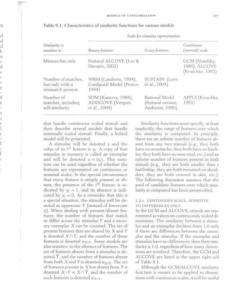
In the Approximately ALCOVE (APPLE) model of Kruschke (1993), that ordering of computations is reversed. First, a similarity is computed on each dimension separately, using an exponentially decaying function of distance within each dimension:

Second, an overall similarity is computed by combining the dimensional similarities via a sigmoid (also known as squashing or logistic) function:

sex, y)

= Sig ( I:>i(X, y);g, e) I

(9.9)

where the gain, g > 0, is the steepness of the sigmoid and e is a threshold that is typically somewhat less than the number of dimensions being summed.

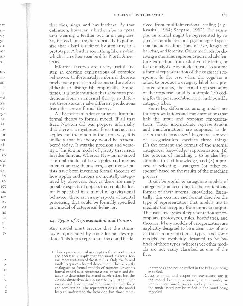
Figure 9 .2 shows a plot of this similarity function, which should be contrasted with the GeM/ALCOVE similarity function shown in Figure 9.1. This similarity function has some attractive characteristics, one being that individual featural matches can have disproportionately strong influence on overall similarity. This is revealed in Figure 9.2 as the "ridges" where either Xl = Yl or X2 = Y2. Another useful property of the similarity function is that self-Similarity (i.e., when Y = x) can vary from exemplar to exemplar if they have different thresholds or gains. In particular, the self-Similarity can be less than 1.0 when the threshold e is , , high. Finally, when there are more dimensions on which the stimuli match, then the similarity is larger. This can be inferred from Equation 9.9: When there are more dimensional Si (x, y) terms contributing to the sum, the overall sex, y) is larger. Thus, APPLE's similarity function operates on continuously scaled stimuli and is affected by the number of matching dimensions, even for identical stimuli. Therefore, it is listed in Table 9.1 in the lower right cell.

When the continuously scaled dimensions assumed by APPLE are reduced to present/absent features represented by 1/0 values, the similarity function can be expressed in terms of the number of matching and differing features. Simplify by assuming C'ti = 1 for all i, then Equations 9.8 and 9.9 imply

seX, Y) = Sig ( n XnY + nxnY

+}(nx~y+ny~x);g,e) (9.10)

where e = 2 .718 is the base of the exponential function. Clearly, this similarity is a function of both the number of matching features and the number of mismatching features .


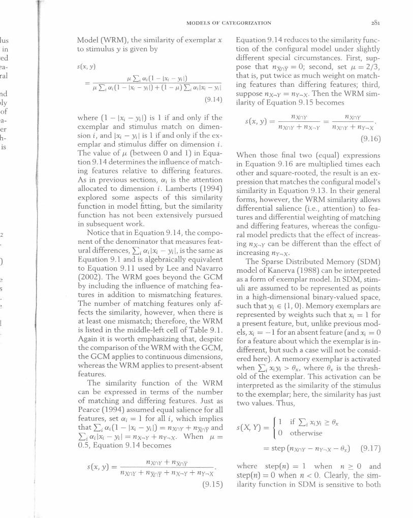
APPLE: g=7, (k1, a=(O.5,O.5)

.. '

.. ' ,.'

,,' ,-

0 .8

a 2- 0.6

II x

52 >; 0.4 x (j)

0.2

0 5

5

-5 -5

Y2 Y1

Figure 9.2. Similarity function in Approximately ALCOVE (APPLE), from Equations 9.8 and 9.9, using specific parameter values indicated in the title of the figure. Compare with Figure 9.1.

2.2.3. NOMINAL SCALE, SENSITIVE TO

DIFFERENCES ONLY

Whereas the GCM, ALCOVE, and APPLE apply to stimuli represented on continuous scales, there are also many models of categorization that apply to stimulus representations composed of nominally scaled dimensions. This section reviews several such models that are sensitive only to stimulus differences, not to stimulus commonalities (analogous to GCM/ ALCOVE). A later sec-' tion addresses similarity functions in which commonalities do have an influence (analogous to APPLE).

Lee and Navarro (2002) discussed a featural ALCOVE model in which stimuli are represented as features derived from additive clustering techniques. Let Xi denote the presence or absence of feature i in stimu-

Ius x, such that Xi = 1 if x has features i, and Xi = 0 otherwise. The distance between exemplar x and stimulus y is given by

d(x, y) = 2.: a i [Xi(l- yJ + (1 - Xi)Yd·

(9 .11 )

Notice in Equation 9.11 that the term inside the square brackets is simply 1 if feature i mismatches and 0 otherwise. The distance is algebraically equivalent to Li ai IXi - Yi I, which is an expression seen before in Equation 9.1 and which will be seen again in Equation 9.14. Lee and Navarro (2002) preferred to express the distance as shown in Equation 9.11 because it suggests discrete values for Xi and Yi rather than continuous

KRUSCHKE

values. Lee and Navarro (2002) then defined similarity as the usual exponentially decaying function of distance. In the special case that C¥i = 1 for all i, the similarity function becomes exactly Equation 9 .7. This similarity function is not sensitive to matching features, so this model is listed in the upper left cell of Table 9.1. Lee and Navarro (2002) collected human learning data for stimuli that were well described by present/absent features, and found that ALCOVE with the featural representation fit the data better than the original continuousscaled ALCOVE.

2.2+ NOMINAL SCALE, SENSITIVE

TO MATCHES

Several models are considered in this section. This section first describes models that assume binary valued (present/absent) features and then moves on to models that assume features with m values. Within each of those, the discussion first addresses models that are sensitive to the number of matching features only when at least one mismatch is present and then addresses models that are sensitive to the number of matching features, even when there are no mismatching features.

Pearce (1987) developed a model in which similarity is a function of both matching and distinctive features. He defined the similarity of two stimuli, X and Y, to be

(X Y) = f(Xn Y)f(Xn Y) s , f(X)f(Y) (9.12)

where f (X) is a monotonic function of the number of features in X and of the individual saliences of the features.

Pearce (1994) proposed a specific version of that function in his configural model of associative learning. First, restrict consideration to a situation where all features are equally salient. Let the number of features in stimulus X be denoted nx. When exemplar X is perceived, its features compete for limited attention, such that each feature is activated to a level 1/.foX. This level of activation implies that the sum of the squared

activations is unity. Every distinct stimulus recruits a copy of that stimulus activation in exemplar memory. Pearce (1994) referred to those exemplars as configurations of features, hence, the moniker of the configural model.

The similarity of a memory exemplar and a stimulus was then defined to be simply the sum over features of the products of the feature activations . Because absent features have zero activation, the sum over all features reduces to a sum over matching present features; hence, the similarity is given by:

seX, Y)

= L _1 __ 1_

iEXnY Fx ..fiiY

1 1 = nXnY----

Fx ..fiiY

[nxnY nxny ] 1/2

- (nxny+nx~y) (nxny+ny~x) .

(9.13)

Notice that the similarity increases when the number of matching features increases, as long as there is at least one differing feature. Hence, the configura 1 model is listed in the middle-left cell of Table 9.1.

Young and Wasserman (2002) compared Pearce's (1994) model and ALCOVE on a task involving learning about stimuli with present/absent features. ALCOVE was not designed for present/absent features, and Pearce's model does not have selective attention. Young and Wasserman (2002) found that neither model accurately captured the learning trends in their set of category structures, but suggested that it might be possible to modify the attentional capacity constraints in the models to address their findings.

Lamberts (1994) explored another similarity function that is sensitive to matching features and distinctive features. Again, consider features that are binary valued, either present or absent, and coded as 1 or 0, respectively. In Lamberts 's Weighted Ratio

Ius LIn

~ed earal

nd )ly of ~a

·er h-is

2

)

5

MODELS OF CATEGORIZATlON

Model (WRM), the similarity of exemplar x to stimulus y is given by

s(x,y)

= I-'-·L ai(l -IXi - yil) + (1 - 1-'-) Li ailXi - yil

(9.14)

where (1 - IXi - Yi I) is 1 if and only if the exemplar and stimulus match on dimension i, and IXi - yil is 1 if and only if the exemplar and stimulus differ on dimension i. The value of fJ.- (between 0 and 1) in Equation 9.14 determines the influence of matching features relative to differing features. As in previous sections, Cii is the attention allocated to dimension i. Lamberts (1994) explored some aspects of this similarity function in model fitting, but the similarity function has not been extensively pursued in subsequent work.

Notice that in Equation 9.14, the component of the denominator that measures featural differences, Li Cii IXi - Yi I, is the same as Equation 9.1 and is algebraically equivalent to Equation 9.11 used by Lee and Navarro (2002). The WRM goes beyond the GeM by including the influence of matching features in addition to mismatching features. The number of matching features only affects the similarity, however, when there is at least one mismatch; therefore, the WRM is listed in the middle-left cell of Table 9.1. Again it is worth emphasizing that, despite the comparison of the WRM with the GeM, the GeM applies to continuous dimensions, whereas the WRM applies to present-absent features.

The similarity function of the WRM can be expressed in terms of the number of matching and differing features. Just as Pearce (1994) assumed equal salience for all features, set Cii = 1 for all i, which implies that Li Cii (1 - IXi - Yi I) = nxnY + nxnY and Li CiilXi - yil = nX~Y + ny~x· When fJ.- = 0.5, Equation 9.14 becomes

() nxnY + nxnY

s x,Y = nXnY + nxny + nX~Y + ny~X

(9.15)

Equation 9.14 reduces to the similarity function of the configural model under slightly different special circumstances. First, suppose that n-xny = 0; second, set fJ.- = 2/3, that is, put twice as much weight on matching features than differing features; third, suppose nX~Y = ny~x. Then the WRM similarity of Equation 9.15 becomes

nXnY sex, y) = ----

nXnY + nX~Y nXnY

(9.16)

When those final two (equal) expressions in Equation 9.16 are multiplied times each other and square-rooted, the result is an expression that matches the configural model's similarity in Equation 9.13. In their general forms, however, the WRM similarity allows differential salience (i.e., attention) to features and differential weighting of matching and differing features, whereas the configural model predicts that the effect of increasing nX~Y can be different than the effect of increasing ny~x.

The Sparse Distributed Memory (SDM) model of Kanerva (1988) can be interpreted as a form of exemplar model. In SDM, stimuli are assumed to be represented as points in a high-dimensional binary-valued space, such thatYi E {I, O}. Memory exemplars are represented by weights such that Xi = 1 for a present feature, but, unlike previous models, Xi = -1 for an absent feature (and Xi = 0 for a feature about which the exemplar is indifferent, but such a case will not be considered here). A memory exemplar is activated when Li XiYi > ex, where ex is the threshold of the exemplar. This activation can be interpreted as the similarity of the stimulus to the exemplar; here, the similarity has just two values. Thus,

if Li Xi Yi ::: ex otherwise

= step (n xny - ny~X - ex) (9.17)

where step(n) = 1 when n::: 0 and step(n) = 0 when n < o. Clearly, the similarity function in SDM is sensitive to both

KRUSCHKE

matching and differing features, and it is listed in the lower-left cell of Table 9.1. SDM has not been extensively applied to many behavioral phenomena, but it is included here as an example of the variety of possible similarity functions .

Verguts et aL (2004) developed a variation of ALCOVE that they called Additive ALCOVE (ADDCOVE) because the first step in its similarity computation is an additive weighting of features. Specifically, suppose a stimulus consists of features Xi. The corresponding exemplar in memory is given

feature weights Wi = Xii JLj xJ = Xi/llxll · When presented with stimulus y, a baseline exemplar activation is computed by adding weighted features as follows:

(9.18)

When x and y consist of 011 bits, Equation 9. 18 becomes

1 a(x, y) = L r.;;-;;

iE)(nY v nx

= nxnd-JitX, (9.19)

which is like the configural model (Equation 9.13), except that here, Yi = I, not lifo·

These baseline activations are then normalized relative to other exemplar activations. Included in the set of other exemplar activations is a novelty detector, which has aN(Y) = ellyll = fowithe close to 1.0, for example, 0.99. The similarity of exemplar x to stimulus y is then given as

sex, y) = a(x, Yl' / [ ~ ark, yl' + aN(Y)']

(9.20)

where the index, k, varies over all exemplars in memory. When x and y consist of all bits,

Equation 9 .20 becomes

sex, y)

- [LK(nKnd.foK)4> + (8.JnY) 4> ]

(nxnd .Jnxny + nX~y )4>

= [LK(nKny/.JnKnY + nK~y) 4> + (8.JnY)4> ] ·

(9.21)

As can be gleaned from Equation 9.2 1, this similarity function depends on both the shared and the distinctive features between the exemplar and the stimulus.

Notice that the similarity function of Equation 9.21 can be asymmetric: sex, y) #s(y, x) when X-, Y #- Y-,X In other words, if a memory exemplar has, say, one feature that a stimulus does not have, but that stimulus has two features that the memory exemplar does not have, then the similarity of the stimulus to the exemplar is different from the similarity of the exemplar to the stimulus. This asymmetry might be useful for addressing analogous asymmetries in human similarity judgments. (Another example of an asymmetric similarity function can be found in Sun, 1995, p. 258.) Interestingly, moreover, the similarity in Equation 9.21 also depends on what other exemplars are currently in memory. Thus, a stimulus might be fairly similar to an exemplar at one moment, but after another highly similar exemplar is added to memory, the similarity to the first exemplar will be reduced.

The SUSTAIN model of Love et aL (2004) employs a similarity function that operates on multivalued (not just binary valued) nominal dimensions. Different nominal dimensions can have different numbers of values. For example, the dimension of marital status might have three values (single, married, divorced), and the dimension of political affiliation might have four values (Democrat, Republican, Green, Libertarian). If dimension i has mi values, then a stimulus is represented by a bit vector of length Li m i

that has l 's in positions of present features and a's elsewhere.

~r

~ 1 )

~n

-e 1-

(-

y

o

n

1

MODELS OF CATEGORIZATiON

In SUSTAIN, what is here being referred to as "exemplars" are not just copies of individual stimuli, but are instead central tendencies of clusters of stimuli. In certain conditions, SUSTAIN could recruit a cluster node for every presented instance and could therefore become a pure exemplar model. The representation for a cluster is also a vector of Li n1i values, but the values are the means (between 0 and 1) of the instances represented by the cluster. The components of the vectors are denoted Xiu, where the subscript indicates the v th element of the i th

dimension. The similarity of a cluster node x to a stimulus y is then defined as

x Lai exp (-.sai L IXiu - Yiul' I U8 ~

(9.22)

where y ::: 0 governs the relative dominance of the most attended dimension over the less attended dimensions. Notice that if x = Y then sex, y) = 1 regardless of how many dimensions are involved.

It should be noted that Love et al. (2004) never asserted that Equation 9.22 is a model of similarity; rather, they simply defined the activation of a cluster node when a stimulus is presented. It is merely by analogy to other models that it is here being called similarity. Moreover, the final activation of cluster nodes in SUSTAIN is another step away: There is competition and then only the winner retains any activation at all. Because the SUSTAIN model incorporates several other mechanisms that distinguish it from other exemplar models, it is not clear which aspects of the specific formalization in Equation 9.22 are central to the model's behavior. The function is described here primarily as an example of how similarity can be defined on multivalued nominal dimensions .

SUSTAIN's similarity function can be related to previous approaches that assumed binary valued features. Suppose that ev-

ery feature is binary valued, suppose that ai = 1 for all features, and suppose that clusters represent single exemplars (so that Xi E {O, 1 D. Then Equation 9.22 becomes

(n xny + nxny) + .!.(nx~Y + ny~x) sex, y) = e

(nxny + nxny) + (nx~y + ny~x) (9.23)

where e = 2.718 is the base of the exponential function. This special case of the similarity function clearly decomposes the influence of matching and differing features. The numerator of this equation appeared before, specifically in Equation 9.10, which expressed the APPLE model when applied to the special case of binary features. The APPLE model compresses the range of that numerator by passing it through a sigmoidal squashing function. The SUSTAIN model compresses the range of that numerator by dividing by the total number of features. However, unlike APPLE, the ratio in SUSTAIN is only sensitive to the number of matching features when there is at least one mismatching feature; hence, SUSTAIN is listed in the center cell of Table 9.l.

Another approach to similarity, and the last that will be considered here, is provided by the rational model of Anderson (1990, 1991). Like SUSTAIN, the rational model recruits cluster nodes as training progresses. In the limit, it can recruit one cluster per (distinct) exemplar and behave much like the GCM (Nosofsky, 1991).

The rational model takes a Bayesian approach, which entails fundamental ontological differences from the previous approaches. (For a discussion of Bayesian models more generally, see Chapter 3 in this volume.) The goal of the rational model is to mimic the probability distribution of features observed in instances. Each cluster node represents the probability of sampling any particular feature value, and the model overall represents the probability of instances as a mixture of cluster-node distributions. But that statement does not capture an important subtlety of the Bayesian

KRUSCHKE

approach: Each cluster node represents an entire distribution of beliefs about possible probabilities of features values.

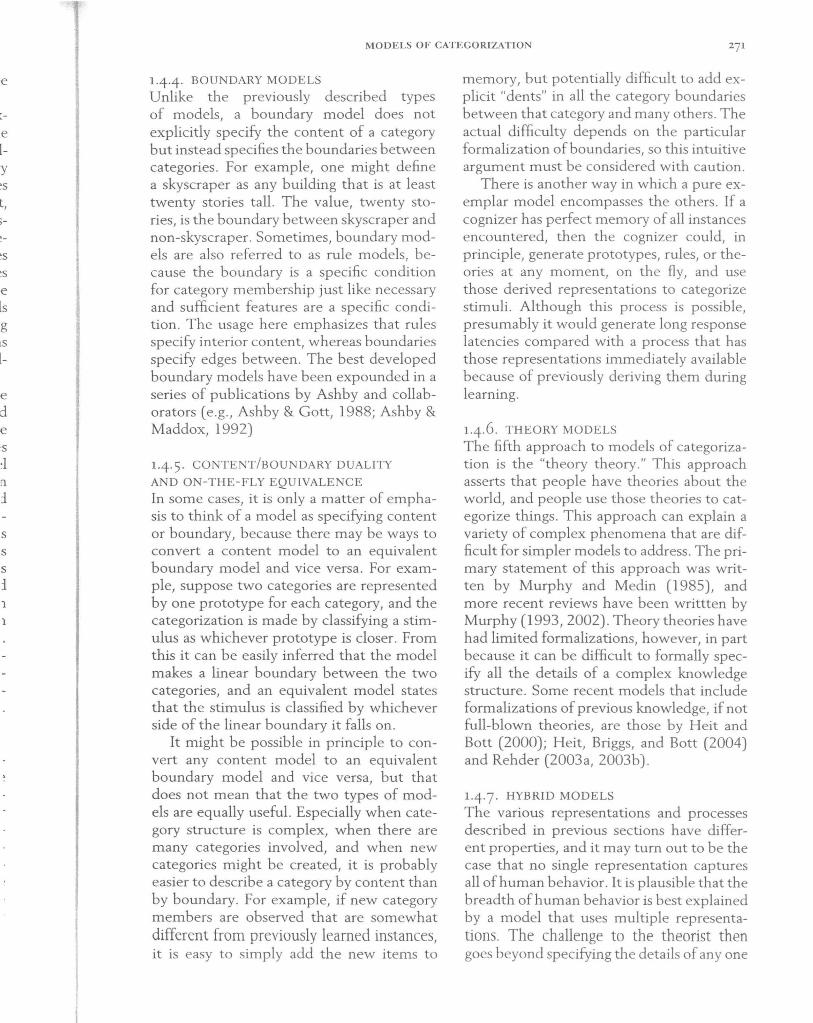
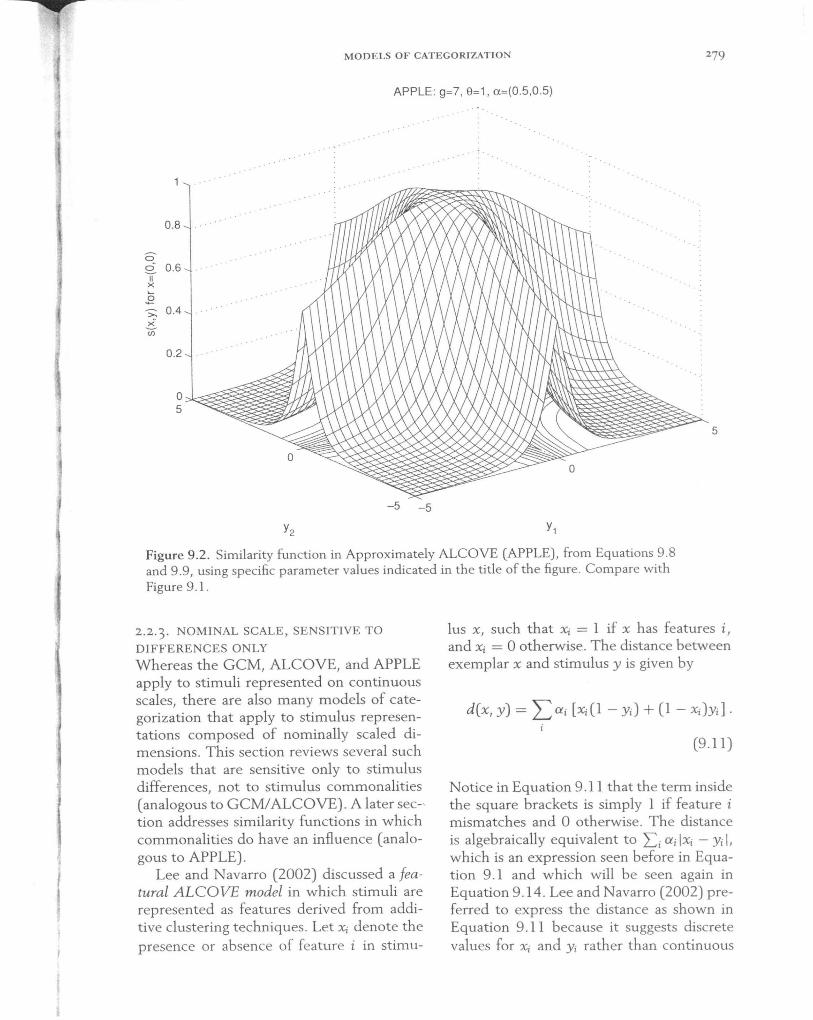
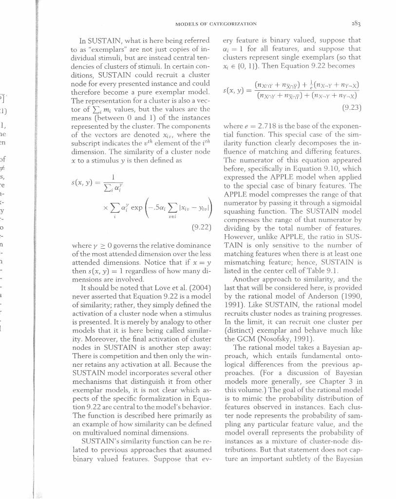
For example, suppose a cluster node is representing the distribution of heads and tails (i.e., the feature values) in a sequence of coin flips (i.e., the instances). Denote the underlying probability of heads as (h and the probability of tails as e2 (= 1 - el). One possible belief about the underlying probability of heads is that e] = 0.5, that is, the coin is fair. But there are other possible beliefs that the coin is biased, such as e] = 0.1 or el = 0.9. The cluster node represents the degree of belief in every possible value of e] and e2. By assumption, the model begins (before seeing any instances) with beliefs spread out uniformly over all possible values of e. Gradually, the model loads up its beliefs onto those values of e that best mimic the observed values, simultaneously reducing its belief in values of e that do not easily predict the observed values. Figure 9.3 illustrates this process of updating belief distributions.

In general, when a feature has V values, any particular belief specifies the probability eu of each of the V feature values. A cluster node represents a degree of belief in every possible particular combination of probabilities. The degree of belief is a distribution over the space of all possible values of el, ... ,ev. Such a distribution could, in principle, be specified in a variety of ways; typically, the speCification of the distribution will involve parameter values. Anderson (1990) uses the Dirichlet distribution, which has parameters, au, one per feature value, that determine the distribution's central tendency and shape. In the earlier example with two scale values (i.e., heads and tails), the Dirichlet distribution has two parameters, al and a2 (and in this case is commonly called the Beta distribution). Examples of the Dirichlet distribution are shown in Figure 9.3. Anderson assumes that clusters begin with unbiased beliefs, parameterized by au = 1 for all values v. With each observation of an instance, the distribution of beliefs is updated according to Bayes' theorem. Conveniently, the updated ("poste-

riar") distribution of beliefs turns out also to be a Dirichlet distribution in which the a parameter of the observed feature value is incremented by one. Again, see the caption of Figure 9.3 for an example of this process. Thus, after m v instances with value v, the parameters of the belief distribution are au = mu + 1.

The value eu is, by definition, the probability that the feature value would be generated by the cluster if the value eu were true. So the cluster's predicted probability of feature value v is the integral over all possible values of eu weighted by the probability of believing it is true. Thus, p( v) = r· -f de]·· ·deveu p(el , "', evla ], ... , av). For the Dirichlet distribution, the integral simplifies to

= (mu + 1) / L (mw + 1). (9.24) 11 '

To reiterate, Equation 9.24 provides the probability that a cluster would generate feature value v within a particular featural dimension.

Stimuli do not usually have just one featural dimension, however. For example, they might have the features of political party, marital status, ethnicity, and so forth. The rational model assumes that, within any cluster, the features are independent of each other. Because of this assumed independence, the probability of observing value VI

on feature 1 in conjunction with value V2

on feature 2, and so forth, is the product of their individual probabilities: P({Vd}) = Ild P(Vd). Anderson used that overall probability of the stimulus as a measure of how similar the stimulus is to the cluster. Formally, for a stimulus y = {Vd} and a cluster x = laUd}, the "similarity" of y to x is

sex, y) = n P(Vd) d

= n mUd + 1 d L w Ed(m w +l)'

(9.25)

also the

le is tion Jro-e v, are

ob-be

'ere lity all

Jb-1= ,} ral

4)

le te al

t

Y

" e y I

:l

t

MODELS OF CATEGORIZATION 285

0 0 0

]i M- a, = 1, a2= 1 ]i M a, = 1, a2 = 2 ]i (") a,=1,a2=3 Q) - Q) Q) a:J ;j- a:J ~ a:J 0

'0 '0 N '0 N

-Q) ::- Q) 0

Q) ~

~ ~ ~ Ol Ol Ol Q) - Q) Q)

0 ~- 0 0 0 0

o I I I I I I 0 0

0.0 0.4 0.8 0.0 0.4 0.8 0.0 0.4 0.8

8, 8, 8,

0 0 0

]i (") a, = 2, a2 = 1 ]i M- a, = 2, a2=2 ]i (") a, = 2, a2=3 Q) Q) - Q) -a:J 0 a:J ;j- a:J

N

~~~ '0 '0 -

~ '0

Q) ~

Q)

~-Q)

Q) ~ ~ 0, Ol Ol Q) Q) - Q)

0 0 0 ~ 0 o_ 0 0 I I I I I I o I I I I I I

0.0 0.4 0.8 0.0 0.4 0.8 0.0 0.4 0.8

8, 8, 8,

0-'-----------------, ]i M - a, = 3, a2 = 2

0-' ________________ -,

]i M - a, = 3, a2 = 3 a, = 3, a2 = 1 Q) -a:J 0_

Q) -

l~=/\ j~~~ o I I I I I I o I I I I I I

0.0 0.4 0.8 0.0 0.4 0.8 0.0 0.4 0.8

8, 8, 8,

Figure 9.3. Each panel corresponds to the state of a cluster node in Anderson's (1990) rational model. Here, the cluster node is representing a single featural dimension that has two possible values. In each panel, the horizontal axis shows el , which indicates the probability that the feature takes on its first value. (Of course, e2 = 1 - e].) The vertical axis indicates the degree of belief in values of e].

Before observing any instances, the cluster begins in the top-left state, believing uniformly in any possible value of el, which is parameterized as al = 1 and a2 = 1. If the first observed instance displays value I, then the cluster node adjusts its distribution of beliefs to reflect that observation, moving to the left-middle state, parameterized as al = 2 and a2 = 1. If the next observed instance displays value 2, then the cluster node changes its beliefs to the center state, parameterized as a] = 2 and a2 = 2. At this point, because 50% of the instances have shown value I, the cluster believes most strongly that e] = 0.50, but because there have only been two observations, beliefs are still spread out over other possible values of el .

Anderson intended this as similarity only metaphorically and not as an actual model of similarity ratings (Anderson, 1990, p. 105).

Consider the special circumstances wherein all dimensions are binary valued and a cluster represents a single exemplar.

When the cluster represents a single exemplar, it implies that mv = 0 for all v but one. If the represented instance occurred r times, then mv = r for the feature value that actually appeared in the instance. In this particular situation, the similarity formula can be expressed in terms of the number of features

KRUSCHKE

that match or mismatch between the cluster and the stimulus. Equation 9.25 becomes

(

r + 1 ) nxny+nxny

Sex, y) = r + 2

(9 .26)

Because similarity of an instance to its corresponding exemplar is influenced by how often the instance has previously appeared, the rational model is listed in the lower-center cell of Table 9.1.

2.2.5 . HYBRID SCALE

Nosofsky and Zaki (2003) proposed a similarity function that incorporates aspects of the standard spatial similarity metric of Equation 9.2 with coefficients that express discrete-feature matching and mismatching. Their hybrid similarity function defined similarity as

Sh(X, y) = CD exp( -c d(x, y)) (9.27)

where C > 1 expresses the boost in similarity from matching features, and 0 < D < 1 expresses the decrease in similarity from distinctive features. Notice in particular that the similarity of an item to itself is C > 1. Nosofsky and Zaki (2003) found that the hybrid-similarity model fit their recognition data very well, whereas the standard similarity function did not.

2.2.6. ATTENTION IN SIMILARITY

Finally, a crucial aspect of similarity that has not been yet emphasized is selective attention to dimensions or features . Most of the models reviewed earlier do explicitly allow for differential weighting of dimensions. Even the SDM model permits differential feature weights (Kanerva, 1988, p. 46). Only the configural model (Pearce, 1994) and the rational model (Anderson, 1990) do not have explicit mechanisms for selective attention.3 This lack of selective at-

3 Anderson (1990, pp. 116- 117) describes a way to differentially weigh the prior importance of each

tention leaves those models unable to generate some well-established learning phenomena, such as the relative ease of categories for which fewer dimensions are relevant (e.g. , Nosofsky et a1., 1994). See Chapter 9 in this volume for a review that emphasizes the role of attention.

2.2.7. SUMMARY OF SIMILARITY

FORMALIZATIO S

One of the contributions of this chapter is a review of these various models of similarity in a common notation to facilitate comparing and contrasting the approaches. In particular, expressions were derived for the similarity functions in terms of the number of matching and mismatching features when the models are applied to the special case of present/absent features, with equal attention on all the features . This restriction to a special case permits a direct comparison of the similarity functions in terms of the influence of the number of features in each stimulus, the number of distinctive features, and so forth.

If nothing else, what can be concluded from the variety of similarity functions reviewed in this section is that the best formal expression of similarity is still an open issue. The shared commitment in this variety is the claim that categorization is based on computing the similarity of the stimulus to exemplars in memory. Although the review of similarity functions has revealed that there are a variety of formalizations that different researchers have found useful in different circumstances, what is lacking is specific guidance regarding which formalization is appropriate for which situation . A general answer to this question is a foundational issue for future research. A thought-provoking review of how people make similarity judgments has been

featural dimension, but this is opposite from learned selective attention. In Anderson's approach, the model begins with strong prior selectivity that subsequently gets overwhelmed with continued learning. But in human learning, the prior state is, presumably, noncommittal regarding selectivity and subsequently gets stronger with continued learning.

~r-

n-, ·or g., 1is )le

is lrnIn he ·er en of nto :m he ch ~S,

ed ·e)r

en ried n-gh ·e

:a-1d is

:h it)n

h. 0-

ed he lat ed lte ived

MODELS OF CATEGO RIZATION

provided by Medin, Goldstone, and Gentner (1993). A perspective on similarity judgment, as a case of Bayesian integration over candidate hypotheses for generalization, has been presented by Tenenbaum and Griffiths (2001 a).

2.3. Learning of Associations

Exemplar models assume that at least three aspects of the model get learned. First, the stimulus exemplars themselves must be stored. This aspect is discussed in a subsequent section. Second, once the exemplars are in memory, the associations between exemplars and category labels must be established. Third, the allocation of attention to stimulus dimensions must be determined. In principle, other aspects of the model could also be adjusted through learning. For example, the steepness of the generalization gradient (e.g., parameter c in Equation 9.2) could be learned, or the decisiveness of choice (e.g., parameter ¢ in Equation 9.36) could be learned. These intriguing possibilities will not be further explored here.

This section focuses on how the associations between exemplars and category labels are learned. Learned attentional allocation can also be implemented as learned associations to attentional gates, and therefore attentional learning is also a topic of this section. (For a discussion of associative learning in humans and animals, see Chapter 22 in this volume.)

Associative strengths can be adjusted many different ways. Perhaps the simplest way is adding a constant increment to the weight whenever both its source and target node are simultaneously activated. More sophisticated schemes include adjusting the weight so that the predicted activation at the target node better matches the true target activation. These and other methods are discussed en route.

2.3.1. CO-OCCURRENCE COUNTING

The GCM establishes associations between exemplars and categories by simply counting the number of co-occurrences. This can be

understood in the context of Equation 9.3, wherein the effective associative influence between exemplar x and response r is N-x, that is, the number of times that response r has occurred with instance x. Somewhat analogously, in SDM (Kanerva, 1988), associative weights from exemplar nodes to output nodes are incremented (by 1) ifboth the exemplar and the output are co-activated, and associative weights are decremented (by 1) if either is active whereas the other is not.

A related approach is taken by the rational model (Anderson, 1990, p. 136). When implemented in a network architecture, the weight from cluster node k to category-label node r can be thought of as p(rlk) = (m,. + 1)/ Le(me + I), where me is the number of times that category label e has co-occurred with an instance of cluster k. Thus, the change in the associative weight is affected only by the co-occurrence of the cluster and the label. (The assignment of the stimulus to the cluster is affected by past learning, however.)

In all these models, regardless of whether the model is classifying a stimulus well or badly, the associative links are incremented the same amount. Other models adjust their weights only to the extent that there is error in performance (as described in the next section).

In none of these models is there learned allocation of selective attention. In the GCM, attention is left as a free parameter that is estimated by fits to data. In some early work (e.g., Nosofsky, 1984), it was assumed that attention is allocated optimally for the categorization, but there was no mechanism suggested for how the subject learns that optimal allocation.

2.3.2. GRADIENT DESCENT ON ERROR

ALCOVE uses gradient descent on error to learn associative weights and attentional strengths. On every trial, the error between the correct and predicted categorization is determined (see Equation 9.4), and then the gradient of that error is computed, followed by adjustments in the direction of the gradient (see Equations 9.5 and 9.6) .

KRUSCHKE

RASHNL also uses gradient descent, iterated to achieve large shifts of attention on single trials.

In the SUSTAIN model of Love et al. (2004), only the winning cluster (exemplar) node learns, and only its output weights learn by gradient descent on categorization error. The dimensional attention strengths and cluster coordinates learn (almost) by gradient ascent on similarity. That is, the attention strengths are adjusted to increase the similarity of the winning cluster node to the stimulus, and the coordinates of the winning cluster node are moved to increase its similarity to the stimulus. The particular formulas used in SUSTAIN for learning attention and cluster coordinates are not exactly gradient ascent on similarity, however. The goal for the remainder of this section is to demonstrate how gradient ascent on similarity yields learning formulas that are much like the ones used in SUSTAIN.

The SUSTAIN model adjusts the winning cluster's coordinates, Xiv, by applying a learning formula from Kohonen (1982) :

(9.28)

where 1] is a constant of proportionality. (The Kohonen learning rule can be derived as gradient ascent on a Gaussian density function with respect to its mean.) Gradient ascent on the winning cluster's similarity, with respect to its coordinates, yields almost the same formula:

o ~Xi v ex --sex, Y)

oXiv

= l]i sgn(yiv - Xiv) (9.29)

where sgn(z) is the sign of z, such that sgn(z) = +1 if z> 0, sgn(z) = -1 if z < 0, and sgn(z) = 0 if z = O. Equation 9.29 involves coefficients 1]i that depend on the dimension i: 1]i = .Sa;+l

exp( -.Sai LVEi IXiv - Yivl)/ Lj a~. To adjust attention, Love et al. (2004,

p. 314, discussion of their Equation 3) consider the gradient of each dimension's individual similarity with respect to atten-

tion, and heuristically use the formula (their Equation 13):

~a · ex exp(-a·d ·) (1 - a ·d ·) ) ) ) ) ) . (9.30)

This can be recognized as a truncated form of gradient ascent on the winning cluster's overall similarity to the stimulus, as follows. Computation of the derivative yields

o ~aj ex -sex, Y)

oaj

= ~laY {exp(-ajdj) L...t t

( Y-l Yd) y-l ( )} x ya j - a j j - ya j s x, Y

(9.31 )

where d j = (1/2) L v; IXj v, - YjuJ In the special circumstances when y = 1 and L i ai = 1, Equation 9.31 reduces to

~aj exexp(-a jd j)( I -a jd j )-s(x,y),

(9.32)

which is very similar to the formula used by Love et al. (2004) .

In summary, although it is not clear that the formulas used by SUSTAIN always increase the similarity of the winning cluster to the stimulus (because the formulas do not implement gradient ascent), the formulas are analogous to true gradient ascent on similarity. The goal of the formulas in SUSTAIN is to increase the winning cluster's representativeness of the instances it wins. True gradient ascent on similarity would be one way to achieve that goal. Notice, however, that increasing the similarity of the winning cluster to the stimulus might not necessarily reduce error in predicting the category label.

2.3.3. SYSTEMATIC OR RANDOM HILL-CLIMBING

Error reduction can be achieved without explicit computation of the gradient. In principle, any method for function optimization could be used. Indeed, if the parameter space is small enough, a dense

_eir

10)

rm ~r's

II[s.

} 1)

he

1d

2)

at n-er )t

as 1-

N

le

le

r, -g y 1.

It

n

e


search of parameter combinations could be undertaken. But when the parameter space is large, as in most learning situations, there are various "hill-climbing" algorithms that probe the error near the current parameter values and creep their way down the error surface (e.g., Press et a1. 1992, pp. 394-455). Some algorithms, for example, numerically estimate the gradient of the error without an explicit formula for the gradient by trying two different values of a parameter, say wand w + ~w; computing the error generated by each value, E and E + ~ E; and approximating the gradient as ~ E / ~ w. The algorithms then use the estimates of gradient (and sometimes also curvature) to make systematic jumps to new parameter values.

Other algorithms do not bother computing the gradient at all and simply probe nearby values of the parameters, changing to those values if the error is reduced. The algorithms differ in how they decide which nearby values to probe. The Stochastic COntext DEpendent Learning (SCODEL) model of Matsuka (2005) is a noisy hill-climbing algorithm for learning associative weights and attention strengths in ALCOVE. SCODEL randomly tries new values that are close to its current values. If a candidate value decreases error, then the value is kept. But even if the candidate value increases error, there is a nonzero probability that the change is kept. This procedure can allow the model to jump over local minima in the error surface and produces large individual differences between different runs of the model that may mimic the large variance seen in human learners.

2.3+ BAYESIAN LEARNING

A rather different approach to learning is taken by Bayesian parameter estimation. In a Bayesian conceptualization, the mind of the learner is conceived to contain a large set of hypotheses, with each hypothesis specifying particular parameter values. Learning does not change the parameter values within each hypothesis. Instead, learning changes how strongly one believes each hypothesis.

This type of idea was encountered earlier in the context of the rational model

(Anderson, 1990). There were various hypotheses about the underlying probabilities, ()v, of encountering feature values v. For example, the model could believe strongly that a feature value v has probability ()v = 0.2 and believe only weakly that the feature value has probability ev = 0 .9. The degree of belief was governed by a parameterized (Dirichlet) distribution, and Bayesian learning adjusted the parameters of the distribution (see the discussion accompanying Figure 9.3).

Instead of entertaining hypotheses about feature probabilities, consider hypotheses about the magnitude of associative weights in an associative network. For example, one might have two hypotheses about an association between an exemplar and a category. Hypothesis H+ specifies an associative weight of + I, and hypothesis H - specifies an associative weight of -1 . At first, one might have no preference for one hypothesis over the other. This state of beliefs can be expressed as p(H+) = .5 and p(H-) = .5. Suppose that a learning trial is then experienced, in which the instance occurs and is taught to be a member of the category. This occurrence is consistent with H+, so beliefs should shift toward H+; perhaps then p(H+) = .9 and p(H-) = .1. Notice that none of the associative weights has changed, but the degree of belief in each one has changed.

A useful property of Bayesian learning is that changes in degree of belief about one hypothesis must affect degree of belief in other hypotheses. This is because it is assumed that the hypotheses in the hypothesis space are mutually exclusive and exhaust all possible hypotheses . So if evidence compels you to believe less strongly in one hypothesis, you must believe more strongly in other hypotheses. Conversely, if evidence makes you believe more strongly in one hypothesis, you must believe less strongly in other hypotheses. There has been much empirical research demonstrating that people are not very accurate Bayesian reasoners (e.g., Edwards, 1968; Van Wallendael & Hastie, 1990). But in simple situations, people do show Bayesian-like trade-offs in

KRUSCHKE

beliefs. For example, when you find an object d'art fallen from its shelf, you might hypothesize that the cause was either the cat or the toddler. When you then see the cat lying on the shelf where the object d' art was, you exonerate the toddler. Conversely, if you learn that the cat has the alibi of having been outside, the toddler is implicated more strongly.

Bayesian learning of associative weights in connectionist networks has been actively explored in recent years (e.g., MacKay, 2003; Neal, 1996). Psychologists have successfully applied other Bayesian models of learning to associative and causal learning paradigms (e.g., Anderson, 1990, 1991; Courville et a1., 2004; Courville, Daw, & Touretzky, 2004; Dayan & Kakade, 2001; Dayan, Kakade, & Montague, 2000; Gopnik et a1., 2004; Sobel, Tenenbaum, & Gopnik, 2004; Steyvers et a1., 2003; Tenenbaum & Griffiths, 2001b, and Chapter 3 in this volume).

In most existing Bayesian models of category learning, the model has a (possibly infinite) set of hypotheses in which each hypothesis constitutes a complete mapping from stimulus to categorical response. Bayesian learning consists of updating the degree of belief in each of these complete mappings. An alternative new approach uses Bayesian updating within successive subcomponents of the mapping Kruschke (2006). For example, a model such as ALCOVE can be thought of as a succession of two components: The first component maps a stimulus to an allocation of attention across stimulus dimensions; the second component maps attentionally weighted similarities to categorical responses (Kruschke, 2003a). In a typical globally Bayesian approach to ALCOVE, a hypothesis would consist of particular weights on the attention in combination with particular weights on category associations, that is, a hypothesis would be a complete mapping from stimulus to response. In a locally Bayesian approach, there are hypotheses about attention weights separate from hypotheses about category association weights, and Bayesian updating occurs separately on the two hypothesis spaces. The hypothesis space re-

garding category associative weights is updated by using the corrective feedback about the categories. But the hypothesis space regarding attention strengths needs target attention values, analogous to the target category values used for the associative weights. The target attention strengths are determined by choosing those values that maximize (or at least improve) the predictive accuracy of the current associative beliefs. Thus, the internal attentional targets are chosen to be maximally consistent with current beliefs, and only then are beliefs updated with respect to external targets . The approach combines the ability of Bayesian updating to exhibit trade-offs among hypotheses, with the ability of selective attention to produce phenomena such as trialorder effects seen in human learning. See Kruschke (2006) for a description of various phenomena addressed by the locally Bayesian approach.

2.4. Exemplar Recruitment

The previous section described learning of associative strengths, assuming that the exemplars were already in memory. But getting those exemplars into memory is itself a learning process. This section describes a variety of exemplar recruitment models.

2+1. NO RECRUITMENT: PRE-LOADED

EXEMPLARS

In SDM (Kanerva, 1988), memory consists of a set of randomly scattered exemplars, but these memory exemplars need not be copies of presented instances . Instead, the memory exemplars are pre-loaded and form a covering map of the stimulus space. This idea influenced the development of ALCOVE . SDM generates interesting behavior because it assumes high-dimensional spaces for input, exemplars, and output.

One interpretation of the GCM assumes that every distinct trial instance is preloaded as an exemplar in memory. This simplification, although expedient for illustrating the power of the model, is logically dissatisfying because it assumes knowledge is in the model before it could have been

5 Up

Ibout :e re~t atcateghts. eter:naxctive liefs.

are cur-up

The ~sian

hytenrialSee var:ally

5 of ex-5et-self ~s a

ists )ut ies )ry )V

lea rEo Ise .n-

.es 'e

nItly ~e

~n


learned. The original ALCOVE model finessed the issue by assuming the stimulus space was initially covered by a random covering map of exemplars as in SDM; that covering map was the impetus for ALCOVE's name. It turned out that fits to selected data sets were affected little by whether a random covering map or a set of pre-loaded exemplars was used, so most reported fits of ALCOVE use the exemplar version .

2+2. INCESSANT RECRUITMENT

Instead of thinking of the GCM as preloading the exemplars and then incrementing their weights on subsequent presentations, the GCM can be thought of as recruiting a new exemplar with every training instance and creating a link that has weight + 1 between the newly recruited exemplar and the correct category node (Nosofsky, Kruschke, & McKinley, 1992, p. 215). The associative weights of exemplars are unaffected by the specifics of subsequent training. In this way, exemplar learning and associative learning occur with the same magnitude on every trial. Denote the tth repetition of instance x by xt , where the superscript is merely an index, not a power. Then Equation 9.3 becomes

p(RI ) = tJR LXER L~x s(xt, y) . y Lr tJr LkEr L~k s(kt, y)

(9.33)

This is formally equivalent to constant increments on the associative weights (via cooccurrence counting), but a benefit is that each instance merely recruits a new exemplar, rather than having to check if there is already an exemplar that matches it.

2+3. NOVELTY DRIVEN RECRUITMENT

The ADDCOVE model (Verguts et al., 2004), described earlier beginning with Equation 9.18, has exemplar recruitment. When a stimulus occurs that does not match an existing exemplar in memory, then a new exemplar is recruited into memory that exactly copies the current stimulus. Notice that this recruitment process is driven by

stimulus novelty alone, regardless of the performance of the model. Thus, if a novel stimulus appears, a new exemplar is recruited even if the novel item is correctly classified by the model (but the newly recruited exemplar might not learn a very large associative weight to the category nodes if there is little error).

2-4+ PERFORMANCE DRIVEN

RECRUITMENT

Incessant recruitment does not solve a basic problem of frequency counting models : They can become entrenched by large numbers of repeated items in early training. If the correct categorization changes, the model can only slowly learn the change by accumulating vast numbers of subsequent countervailing exemplars. People, however, are quick to relearn after shifts in categories. One solution to this problem is to allow the exemplars to be probabilistically forgotten (e.g., Estes, 1994, p. 63) or for the associative strengths to decay (Nosofsky et al., 1992). In either of those approaches, the initiallearning of any exemplar is full strength. As an alternative new approach, suppose that the initial learning of exemplars should depend on the current performance of the model. An exemplar should be recruited for a stimulus depending on the degree of error generated on that stimulus. 4 When there is a large error, there should be a high probability of recruiting an exemplar. When there is a small error, there should be a small probability of recruiting an exemplar. A challenge to this proposed approach is that probabilistic mappings would continually generate error and endlessly recruit exemplars.

The SUSTAIN model of Love et al. (2004) recruits new cluster nodes under certain conditions, depending on the type of training. For supervised training, that is, when category labels are provided as feedback, a new cluster node is recruited when an instance is presented for which the

4 Previous exemplar theorists have described probabilistic remembering of features or exemplars (e.g., Hintzman, 1986, 1988), but not such that the probability depends on the momentary accuracy of the model.

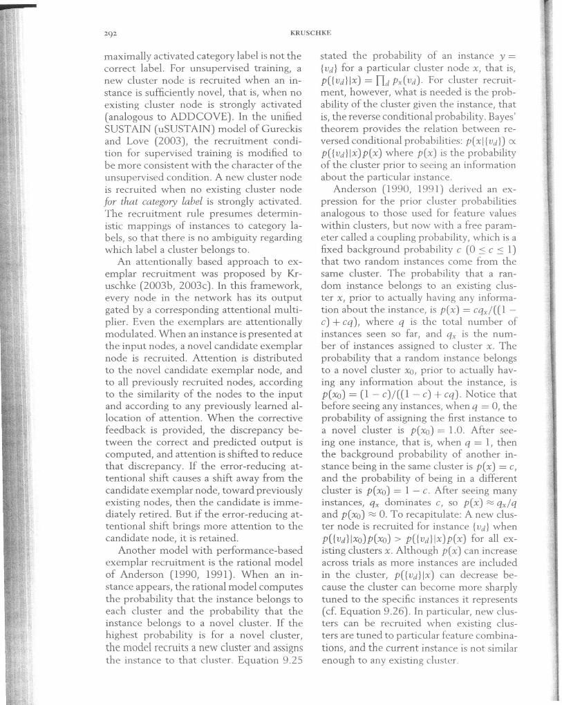
KRUSCHKE

maximally activated category label is not the correct label. For unsupervised training, a new cluster node is recruited when an instance is sufficiently novel, that is, when no existing cluster node is strongly activated (analogous to ADDCOVE). In the unified SUSTAIN (uSUSTAIN) model of Gureckis and Love (2003), the recruitment condition for supervised training is modified to be more consistent with the character of the unsupervised condition. A new cluster node is recruited when no existing cluster node for that category label is strongly activated. The recruitment rule presumes deterministic mappings of instances to category labels, so that there is no ambiguity regarding which label a cluster belongs to.

An attention ally based approach to exemplar recruitment was proposed by Kruschke (2003b, 2003c). In this framework, every node in the network has its output gated by a corresponding attentional multiplier. Even the exemplars are attention ally modulated. When an instance is presented at the input nodes, a novel candidate exemplar node is recruited. Attention is distributed to the novel candidate exemplar node, and to all previously recruited nodes, according to the similarity of the nodes to the input and according to any previously learned allocation of attention. When the corrective feedback is provided, the discrepancy between the correct and predicted output is computed, and attention is shifted to reduce that discrepancy. If the error-reducing attentional shift causes a shift away from the candidate exemplar node, toward previously existing nodes, then the candidate is immediately retired. But if the error-reducing attentional shift brings more attention to the candidate node, it is retained.

Another model with performance-based exemplar recruitment is the rational model of Anderson (1990, 1991). When an instance appears, the rational model computes the probability that the instance belongs to each cluster and the probability that the instance belongs to a novel cluster. If the highest probability is for a novel cluster, the model recruits a new cluster and assigns the instance to that cluster. Equation 9.25

stated the probability of an instance y = {Vd} for a particular cluster node x, that is, p({Vd} Ix) = Od Px(Vd)· For cluster recruitment, however, what is needed is the probability of the cluster given the instance, that is, the reverse conditional probability. Bayes' theorem provides the relation between reversed conditional probabilities: p(xl {Vd}) ex p({vd}lx)p(x) where p(x) is the probability of the cluster prior to seeing an information about the particular instance.

Anderson (1990, 1991) derived an expression for the prior cluster probabilities analogous to those used for feature values within clusters, but now with a free parameter called a coupling probability, which is a fixed background probability c (0 :s c :s 1) that two random instances come from the same cluster. The probability that a random instance belongs to an existing cluster x, prior to actually having any information about the instance, is p(x) = cqx/((l -c) + cq), where q is the total number of instances seen so far, and qx is the number of instances assigned to cluster x. The probability that a random instance belongs to a novel cluster XO, prior to actually having any information about the instance, is p(XO) = (1 - c)/((l - c) + cq). Notice that before seeing any instances, when q = 0, the probability of assigning the first instance to a novel cluster is p(XO) = 1.0. After seeing one instance, that is, when q = I, then the background probability of another instance being in the same cluster is p(x) = c, and the probability of being in a different cluster is p(XO) = 1 - c. After seeing many instances, qx dominates c, so p(x) ~ qx/q and p(xo) ~ O. To recapitulate: A new cluster node is recruited for instance {Vd} when p({vd}lxo)p(xo) > p({vd}lx)p(x) for all existing clusters x. Although p(x) can increase across trials as more instances are included in the cluster, p({vd}lx) can decrease because the cluster can become more sharply tuned to the specific instances it represents (cf. Equation 9.26). In particular, new clusters can be recruited when existing clusters are tuned to particular feature combinations, and the current instance is not similar enough to any existing cluster.

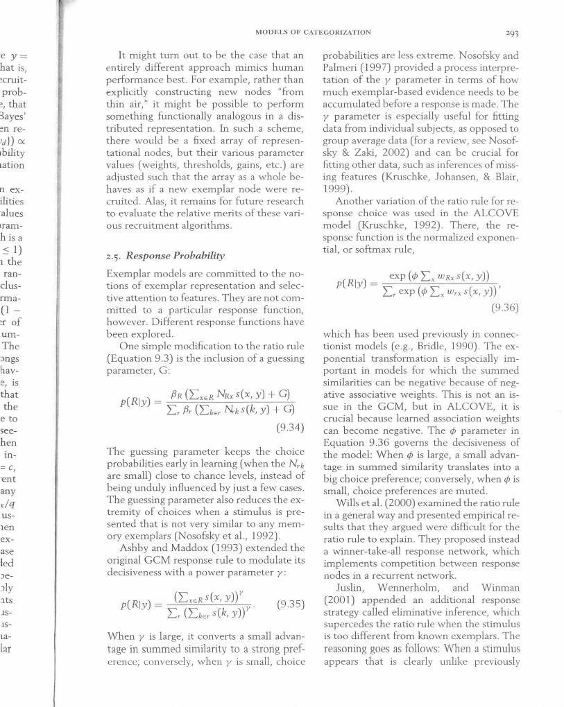
ey= hat is, ~cruit

prob~, that 3ayes' :on reid}) ex Ibility lation

n exilities 'alues Iramh is a :s I)

1 the ran

clusrma-(I -~r of .umThe :mgs have, is that the

e to seehen In-

= c, 'ent any x/q .uslen exase led Je

Jly :Its .lS

.lS

la-tar


It might turn out to be the case that an entirely different approach mimics human performance best. For example, rather than explicitly constructing new nodes "from thin air," it might be possible to perform something functionally analogous in a distributed representation. In such a scheme, there would be a fixed array of representational nodes, but their various parameter values (weights, thresholds, gains, etc .) are adjusted such that the array as a whole behaves as if a new exemplar node were recruited. Alas, it remains for future research to evaluate the relative merits of these various recruitment algorithms.

2.5. Response Probability

Exemplar models are committed to the notions of exemplar representation and selective attention to features. They are not committed to a particular response function, however. Different response functions have been explored.

One simple modification to the ratio rule (Equation 9.3) is the inclusion of a guessing parameter, G:

p(RIY) = f3R (LxER NRx sex, y) + G) Lr f3r (LkEr Nk s (k, y) + G)

(9.34)

The guessing parameter keeps the choice probabilities early in learning (when the Nrk

are small) close to chance levels, instead of being unduly influenced by just a few cases. The guessing parameter also reduces the extremity of choices when a stimulus is presented that is not very similar to any memory exemplars (Nosofsky et aI., 1992).

Ashby and Maddox (1993) extended the original GCM response rule to modulate its decisiveness with a power parameter y:

p(RIY) = (LxER sex, y)r y .

Lr (LkEr s(k, y)) (9.35)

When y is large, it converts a small advantage in summed similarity to a strong preference; conversely, when y is small, choice

probabilities are less extreme. Nosofsky and Palmeri (1997) provided a process interpretation of the y parameter in terms of how much exemplar-based evidence needs to be accumulated before a response is made. The y parameter is especially useful for fitting data from individual subjects, as opposed to group average data (for a review, see Nosofsky & Zaki, 2002) and can be crucial for fitting other data, such as inferences of missing features (Kruschke, Johansen, & Blair, 1999).

Another variation of the ratio rule for response choice was used in the ALCOVE model (Kruschke, 1992). There, the response function is the normalized exponential, or softmax rule,

p(RIY) = exp (¢ Lx WRx sex, y)) Lr exp (¢ Lx Wrx sex, y))'

(9.36)

which has been used previously in connectionist models (e.g., Bridle, 1990) . The exponential transformation is especially important in models for which the summed similarities can be negative because of negative associative weights. This is not an issue in the GCM, but in ALCOVE, it is crucial because learned association weights can become negative. The ¢ parameter in Equation 9.36 governs the decisiveness of the model: When ¢ is large, a small advantage in summed similarity translates into a big choice preference; conversely, when ¢ is small, choice preferences are muted.

Wills et a1. (2000) examined the ratio rule in a general way and presented empirical results that they argued were difficult for the ratio rule to explain. They proposed instead a winner-take-all response network, which implements competition between response nodes in a recurrent network.

Juslin, Wennerholm, and Winman (2001) appended an additional response strategy called eliminative inference, which supercedes the ratio rule when the stimulus is too different from known exemplars. The reasoning goes as follows: When a stimulus appears that is clearly unlike previously

294 KRUSCHKE

learned stimuli, then the response given to it should also be unlike previously learned responses. That is, for an unknown stimulus, eliminate the known categories, and guess at random from the remaining categories. There clearly are circumstances in which people will spontaneously use this strategy (Juslin et al., 2001; Kruschke & Bradley, 1995), but its impact on categorization phenomena more broadly has not been demonstrated (Kruschke, 200 1 b). More generally, however, this raises the point that there are many possible response strategies that people could use, in addition to or instead of the ratio rule.

2.6. Response Time and Choice as a Function of Time

The GCM has no temporal dynamics within or across trials. ALCOVE and RASHNL have dynamics across trials because they learn, but they have no dynamics within trials. Thus, these models make no predictions about response times after onset of a stimulus.

The Exemplar-Based Random Walk model (EBRW; Nosofsky & Palmeri, 1997; Nosofsky & Stanton, 2005) addresses the dynamics of the response process. In the EBRW, exemplars are conceived to be instantly and fully activated by the onset of the stimulus, but then the response is generated by an iterative race to cross response thresholds for each category. Think of each category as having its own horse, racing to cross its response threshold. The race is conceptualized as a series of brief moments of time. In each moment of time, a spinner is spun that points to one of the exemplars at random. The pOinted-at exemplar belongs to one of the categories, and the horse for that category moves ahead one unit toward its response threshold (and the other horses move back one unit). The probability of the spinner pointing to an exemplar, that is, the amount of space an exemplar gets on the spinner, is proportional to the exemplar's similarity to the stimulus. More exactly, the EBRW is applied to two-category situations, and when one horse is moved ahead, the other horse is moved backward.

It is as if there is just one horse, moving either toward one threshold for category A or moving in the opposite direction toward the threshold for category B. The response time is assumed to be proportional to the number of iterations needed until a category threshold is crossed. If the response thresholds for A and Bare y units away from the starting position (in opposite directions), then the probability of choosing category A turns out to be exactly the choice rule described earlier in Equation 9.35 (for a derivation, see Nosofsky & Palmeri, 1997).

Other models of response dynamics include models with recurrent activation and lateral inhibition (Usher & McClelland, 2001; Wills et al., 2000). These models are based on different assumptions than the diffusion/race model assumptions of EBRW. Usher and McClelland (2001) compared the recurrent activation approach with the diffusion model approach (but not the EBRW itself). Wills et al. (2000) applied a winner-take-all recurrent activation network to responses in category learning, but their emphasis was response proportions, not response times.

The EBRW has been applied to domains with integral dimensions, where it is not unreasonable to suppose that exemplars are activated in one fell swoop. When stimulus dimensions are separable, however, then issues about the temporal processing of dimensions loom large. The EBRW was intended primarily as a model of response time dynamics and not so much as a model of perceptual dynamics.

The Extended Generalized Context Model (EGCM) of Lamberts (1995, 1997, 2000) addresses the dynamics of exemplar processing, not just response processing. In the EGCM (Lamberts, 1995, 1998), similarity is a function of time:

set, x, y) = exp (-c ~ ", [n, (t)l" - y, Il) (9.37)

where Ct.; is the utility of dimension i for the categorization, just as in the GCM or ALCOVE, but a new term, Jri(t), is the

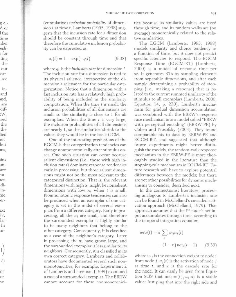
g eiAor 1 the time :lber esh; for ting the out ear-see

mand md, are

dif~W. .red the the lied letbut

uns .Inare lU

Len

diinne er-

~xt

}7, lar In :li -

7)

or or 1e


( cumulative) inclusion probability of dimension i at time t. Lamberts (1995, 1998) suggests that the inclusion rate for a dimension should be constant through time and that therefore the cumulative inclusion probability can be expressed as

Jri(t) = 1 - exp( -qit) (9.38)

where qi is the inclusion rate for dimension i. The inclusion rate for a dimension is tied to its physical salience, irrespective of the dimension's relevance for the particular categorization. Notice that a dimension with a fast inclusion rate has a relatively high probability of being included in the similarity computation. When the time t is small, the inclusion probabilities of all dimensions are small, so the similarity is close to 1 for all exemplars. When the time t is very large, the inclusion probabilities of all dimensions are nearly 1, so the similarities shrink to the values they would be in the basic GCM.

One of the interesting predictions of the EGCM is that categorization tendencies can change nonmonotonically after stimulus onset. One such situation can occur because salient dimensions (i .e., those with high inclusion rates) dominate response tendencies early in processing, but those salient dimensions might not be the most relevant to the categorical distinction. That is, the relevant dimensions with high ai might be nonsalient dimensions with low Jri when t is small. Nonmonotonic response tendencies can also be produced when an exemplar of one category is set in the midst of several exemplars from a different category. Early in processing, all the Jri are small, and therefore the surrounded exemplar is highly similar to its many neighbors that belong to the other category. Consequently, it is classified as a case of the neighbor's category. Later in processing, the Jrj have grown large, and the surrounded exemplar is less similar to its neighbors. Consequently, it is classified in its own correct category. Lamberts and collaborators have documented several such nonmonotonicities; for example, Experiment 2 of Lamberts and Freeman (1999) examined a case of a surrounded exemplar. The EBRW cannot account for these nonmonotonici-

ties because its similarity values are fixed through time, and its random walks are (on average) monotonically related to the relative similarities.

The EGCM (Lamberts, 1995, 1998) models similarity and choice tendency as a function of time, but it does not predict specific latencies to respond. The EGCM Response Time (EGCM-RT) (Lamberts, 2000) is a model of response time per se. It generates RTs by sampling elements from separable dimensions, and after each sample determining a probability of stopping (i.e., making a response) that is related to the current summed similarity of the stimulus to all exemplars (Lamberts, 2000, Equation 14, p. 230). Lambert's mechanism for gradual dimension accumulation was combined with the EBRW's response race mechanism into a model called "EBRW with perceptual encoding" (EBRW-PE) by Cohen and Nosofsky (2003). They found comparable fits to data by EBRW-PE and EGCM-RT, and suggested that although future experiments might better distinguish the models, the random-walk response mechanism in the EBRW-PE is more thoroughly studied in the literature than the stopping-rule mechanism in EGCM-RT. Future research will have to explore potential differences between the models; but there are yet other possibilities for dynamic mechanisms to consider, described next.

In the connectionist literature, processing analogous to Lamberts's inclusion rate can be found in McClelland's cascaded activation approach (McClelland, 1979) . That approach assumes that the i th node's net input accumulates through time, according to the temporal integration equation

neti(t) = K L w;jaj(t) j

(9.39)

where Wij is the connection weight to node i from node j, aj(t) is the activation of node j at time t, and K is the cascade rate for the node. It can easily be seen from Equation 9.39 that net; = Lj wija j is a stable value: Just plug that into the right side and

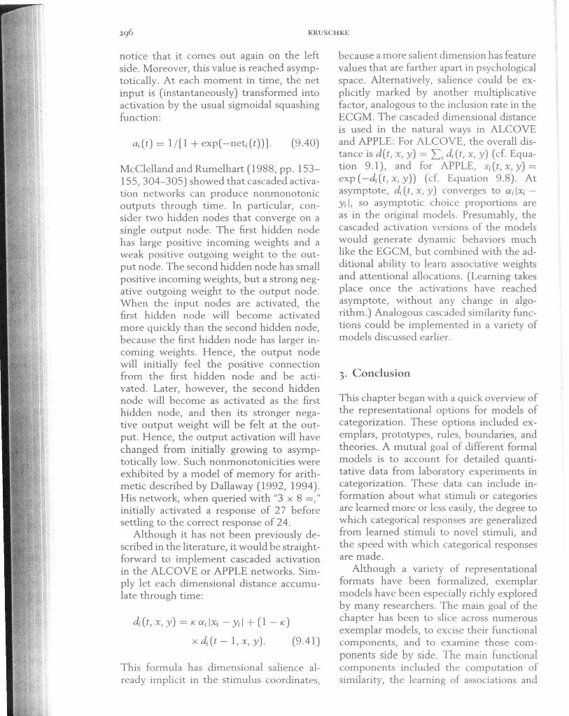
KRUSCHKE

notice that it comes out again on the left side. Moreover, this value is reached asymptotically. At each moment in time, the net input is (instantaneously) transformed into activation by the usual sigmoidal squashing function:

Q.j(t) = 1/[1 +exp(-net1(t))]. (9.40)

McClelland and Rumelhart (1988, pp. 153-155,304-305) showed that cascaded activation networks can produce nonmonotonic outputs through time. In particular, consider two hidden nodes that converge on a single output node. The first hidden node has large positive incoming weights and a weak positive outgoing weight to the output node. The second hidden node has small positive incoming weights, but a strong negative outgoing weight to the output node. When the input nodes are activated, the first hidden node will become activated more quickly than the second hidden node, because the first hidden node has larger incoming weights. Hence, the output node will initially feel the positive connection from the first hidden node and be activated. Later, however, the second hidden node will become as activated as the first hidden node, and then its stronger negative output weight will be felt at the output. Hence, the output activation will have changed from initially growing to asymptotically low. Such nonmonotonicities were exhibited by a model of memory for arithmetic described by Dallaway (1992, 1994). His network, when queried with "3 x 8 =," initially activated a response of 27 before settling to the correct response of 24.

Although it has not been previously described in the literature, it would be straightforward to implement cascaded activation in the ALCOVE or APPLE networks. Simply let each dimensional distance accumulate through time:

c4(t, x, y) = K adXi - Yil + (1 - K)

X c4(t - I, x, y). (9.41)

This formula has dimensional salience already implicit in the stimulus coordinates,

because a more salient dimension has feature values that are farther apart in psychological space. Alternatively, salience could be explicitly marked by another multiplicative factor, analogous to the inclusion rate in the ECGM. The cascaded dimensional distance is used in the natural ways in ALCOVE and APPLE: For ALCOVE, the overall distance is d(t, x, y) = Li c4(t, x, y) (cf. Equation 9.1), and for APPLE, Si(t,x,y)= exp(-c4(t,x,y)) (cf. Equation 9.8). At asymptote, c4 (t, x, y) converges to ai IXi -Yi I, so asymptotic choice proportions are as in the original models. Presumably, the cascaded activation versions of the models would generate dynamic behaviors much like the EGCM, but combined with the additional ability to learn associative weights and attentional allocations. (Learning takes place once the activations have reached asymptote, without any change in algorithm.) Analogous cascaded similarity functions could be implemented in a variety of models discussed earlier.

3. Conclusion

This chapter began with a quick overview of the representational options for models of categorization. These options included exemplars, prototypes, rules, boundaries, and theories. A mutual goal of different formal models is to account for detailed quantitative data from laboratory experiments in categorization. These data can include information about what stimuli or categories are learned more or less easily, the degree to which categorical responses are generalized from learned stimuli to novel stimuli and , the speed with which categorical responses are made.

Although a variety of representational formats have been formalized, exemplar models have been especially richly explored by many researchers. The main goal of the chapter has been to slice across numerous exemplar models, to excise their functional components, and to examine those components side by side. The main functional components included the computation of similarity, the learning of associations and

lture 'gical ~ exative 1 the ance )VE . disqua-y) =

At Xj

are the

,dels lUch ~ adghts akes :hed 19olncyof

vof ; of exand nal nti; in in

:ies ~ to ~ed

md ses

nal .Jar oed :he IUS

1a1 m

lal of nd


attention, the recruitment of exemplars, the determination of response probability, and the generation of response times. This dissection revealed a variety of formalizations available for expressing any given psychological process . The analysis also suggested numerous directions for novel research .

References

Anderson, J. A., Silverstein, J. W ., Ritz, S. A., & Jones, R. S. (1977) . Distinctive features, categorical perception, and probability learning: Some applications of a neural model. Psychological Review, 84(5), 413-451.

Anderson, J. R. (1990). The adaptive character of thought. Hillsdale, NJ: Lawrence Erlbaum.

Anderson, J. R. (1991). The adaptive nature of human categorization. Psychological Review, 98(3),409-429.

Ashby, F. G., Alfonso-Reese, L. A., Turken, A. U., & Waldron, E. M. (1998). A neuropsychological theory of multiple systems in category learning. Psychological Review, 105(3) , 442-481.

Ashby, F. G., & Gott, R. E. (1988). Decision rules in the perception and categorization of multidimensional stimuli. Journal of Experimental Psychology: Learning, Memory, and Cognition, 14(1),33-53.

Ashby, F. G., & Maddox, W. T. (1992). Complex decision rules in categorization: Contrasting novice and experienced performance. Journal of Experimental Psychology: Human Perception & Performance, 18, 50-71.

Ashby, F. G ., & Maddox, W. T. (1993). Relations between prototype, exemplar and decision bound models of categorization. Journal of Mathematical Psychology, 37, 372-400.

Ashby, F. G., & Maddox, W. T. (2005). Human category learning. Annual Review of Psychology, 56, 149-178.

Bourne, L. E. (1966) . Human conceptual behavior. Boston: Allyn and Bacon .

Bridle, J. S. (1990). Probabilistic interpretation of feedforward classification network outputs, with relationships to statistical pattern recognition . In F. Fogelman Soulie & J. Herault (Eds.), Neurocomputing: Algorithms, architectures and applications (pp. 227-236). New York: Springer-Verlag.

Bruner, J. S., Goodnow, J. 1., & Austin , C. A. (1956). A study of thinking. New York: Wiley.

Busemeyer, J. R., Dewey, G. I., & Medin, D. L. (1984) . Evaluation of exemplar-based generalization and the abstraction of categorical information. Journal of Experimental Psychology: Learning, Memory, & Cognition, 10(4), 638-648.

Carpenter, G. A., & Grossberg, S. (1987). A massively parallel architecture for a selforganizing neural pattern recognition machine. Computer Vision, Graphics, and Image Processing, 37, 54-115.

Cohen, A. L., & Nosofsky, R. M. (2003). An extension of the exemplar-based random-walk model to separable-dimension stimuli. Journal of Mathematical Psychology, 47, 150-165.

Courville, A. c., Daw, N. D., Gordon, G. J., & Touretzky, D . S. (2004). Model uncertainty in classical conditioning. In S. Thrun, L. K. Saul, & B. Scholkopf (Eds.), Advances in neural information processing systems (Vol. 16, pp. 977-984). Cambridge, MA: MIT Press.

Courville, A. c., Daw, N . D., & Touretzky, D. S. (2004). Similarity and discrimination in classical conditioning: A latent variable account. In L. K. Saul, Y. Weiss, & L. Bottou (Eds.), Advances in neural information processing systems (Vol. 17). Cambridge, MA: MIT Press.

Dallaway, R. (1992) . Memory for multiplication facts. In J. K. Kruschke (Ed.), Proceedings of the Fourteenth Annual Conference of the Cognitive Science Society (pp. 558-563). Hillsdale, NJ: Lawrence Erlbaum.

Dallaway, R. (1994). Dynamics of arithmetic: A connectionist view of arithmetic skills. Unpublished doctoral dissertation, University of Sussex at Brighton, UK.

Dayan, P., & Kakade, S. (2001) . Explaining away in weight space. In T. Leen, T. Dietterich, & V. Tresp (Eds.), Advances in neural information processing systems (Vol. 13, pp. 451-457). Cambridge, MA: MIT Press.

Dayan, P., Kakade, S., & Montague, P. R. (2000). Learning and selective attention. Nature Neuroscience, 3, 1218-1223.

Edelman, S., & Weinshall, D. (1991). A selforganizing multiple-view representation of 3D objects. Biological Cybernetics, 64, 209-219.

Edwards, W. (1968) . Conservatism in human information processing. In B. Kleinmuntz (Ed.), Formal representation of human judgment. New York: Wiley.

Erickson, M. A., & Kruschke, J. K. (1998). Rules and exemplars in category learning. Journal of Experimental Psychology: General, 127(2), 107-140.

KRUSCHKE

Erickson, M. A., & Kruschke, J. K (2002). Rulebased extrapolation in perceptual categorization. Psycho nomic Bulletin & Review, 9(1), 160-168.

Estes, W. K (1993). Models of categorization and category learning. In G. Nakamura, R. Taraban, & D. L. Medin (Eds.), Psychology of learning and motivation (Vol. 29, pp. 15-56). San Diego, CA: Academic Press.

Estes, W. K. (1994). Classification and cognition. New York: Oxford University Press.

Gati, 1., & Tversky, A. (1984). Weighting common and distinctive features in perceptual and conceptual judgments. Cognitive Psychology, 16(3),341-370.

Gluck, M. A., & Bower, G . H. (1988). From conditioning to category learning: An adaptive network model. Journal of Experimental Psychology: General, II 7(3),227-247.

Goldstone, R. L., & Kersten, A. (2003). Concepts and categorization. In A. F. Healy & R. W. Proctor (Eds.), Comprehensive handbook of psychology, volume 4: Experimental psychology (pp. 599-621). Hoboken, NJ: Wiley.

Gopnik, A., Glymour, c., Sobel, D. M., Schulz, L. E., Kushnir, T., & Danks, D. (2004). A theory of causal learning in children: Causal maps and Bayes nets. Psychological Review, Ill, 3-32.

Gureckis, T. M., & Love, B. C. (2003). Human unsupervised and supervised learning as a quantitative distinction. International Journal of Pattern Recognition and Artificial Intelligence, 17(5), 885-90l.

Heit, E., & Bott, L. (2000). Knowledge selection in category learning. In D. L. Medin (Ed.), The psychology of learning and motivation (Vol. 39, pp. 163-199). San Diego, CA: Academic Press.

Heit, E., Briggs, J., & Bott, L. (2004). Modeling the effects of prior knowledge on learning incongruent features of category members. Journal of Experimental Psychology: Learning, Memory and Cognition, 30(5), 1065-1081.

Hintzman, D. L. (1986). "Schema abstraction" in a multiple-trace memory model. Psychological Review, 93, 411-428.

Hintzman, D. L. (1988). Judgments of frequency and recognition memory in a multipletrace memory model. Psychological Review, 95, 528-551.

Hurwitz, J. B. (1994). Retrieval of exemplar and feature information in category learning. Journal of Experimental Psychology: Learning, Memory and Cognition, 20, 887-903.

Juslin, P., Wennerholm, P., & Winman, A. (2001). High level reasoning and base-rate use: Do we need cue competition to explain the inverse base-rate effectJ Journal of Experimental Psychology: Learning, Memory and Cognition, 27, 849-871.

Kalish, M. L., Lewandowsky, S., & Kruschke, J. K. (2004). Population of linear experts: Knowledge partitioning and function learning. Psychological Review, 111(4) , 1072-1099.

Kanerva, P. (J 988). Sparse distributed memory. Cambridge, MA: MIT Press.

Kohonen, T. (1982). Self-organized formation of topologically correct feature maps. Biological Cybernetics, 43, 59-69.

Kruschke, J. K (1992) . ALCOVE: An exemplarbased connectionist model of category learning. Psychological Review, 99, 22-44.

Kruschke, J. K. (1993) . Human category learning: Implications for backpropagation models. Connection Science, 5, 3-36.

Kruschke, J. K. (2001a). Toward a unified model of attention in associative learning. Journal of Mathematical Psychology, 45, 812-863.

Kruschke, J. K. (2001b). The inverse base rate effect is not explained by eliminative inference. Journal of Experimental Psychology: Learning, Memory and Cognition, 27, 1385-1400.

Kruschke, J. K (2003a). Attention in learning. Current Directions in Psychological Science, 12, 171-175.

Kruschke, J. K. (2003b, April). Attentionallymodulated exemplars and exemplar mediated attention. Keynote Address to the Associative Learning Conference, University of Cardiff, Wales.

Kruschke, J. K (2003c, May) . Attentionally modulated exemplars and exemplar mediated attention. Invited talk at the Seventh International Conference on Cognitive and Neural Systems, Boston University. Boston, MA.

Kruschke, J. K. (2005). Category learning. In K. Lamberts & R. L. Goldstone (Eds.), The handbook of cognition (pp . 183-201). London: Sage.

Kruschke, J. K (2006) . Locally Bayesian learning with applications to retrospective revaluation and highlighting. Psychological Review, 113,677-699.

Kruschke, J. K, & Bradley, A. L. (1995). Extensions to the delta rule for associative learning (Indiana University Cognitive Science Research Report # 141). Retrieved June 26, 2007, from http://www .indiana.edulkruschke/articlesl KruschkeB 1995.pdf.

1\. te in x-ui

:e, ts: ,g.

y.

of :al

Irn-

n-Is.

leI of

~f-

:e. Lg,

.g. 2,

d-u-ve

ff,

d-n-

.al IS,

In he n:

n-Il-'J) ,

n-

n-:h m /


Kruschke, J. K., & Erickson, M. A . (1994). Learning of rules that have high-frequency exceptions: New empirical data and a hybrid connectionist model. In Proceedings of the Sixteenth Annual Conference of the Cognitive Science Society (pp. 514-519) . Hillsdale, NJ: Lawrence Erlbaum.

Kruschke, J. K. , & Johansen, M . K. (1999). A model of probabilistic category learning. Journal of Experimental Psychology: Learning, Memory and Cognition, 25(5) , 1083-1119.

Kruschke, J. K, Johansen, M. K. , & Blair, N. J. (1999, June) . Exemplar model account of inference learning. Unpublished manuscript. Retrieved June 26, 2007, from http://www. indiana.edulkruschke/articles/ KruschkeJB 1999. pdf.

Kruskal, J. B. (1964). Nonmetric multidimensional scaling: A numerical method. Psychometrika,29, 115-129.

Lamberts, K. (1994). Flexible tuning of similiarity in exemplar-based categorization . Journal of Experimental Psychology: Learning, Memory, and Cognition, 20(5),1003-1021.

Lamberts, K (1995). Categorization under time pressure. Journal of Experimental Psychology: General, 124, 161-180.

Lamberts, K. (1997). Process models of categorization. In K. Lamberts & D. Shanks (Eds.), Knowledge, concepts and categories (pp. 371-403). Cambridge, MA: MIT Press.

Lamberts, K. (1998) . The time course of categorization. Journal of Experimental Psychology: Learning, Memory, and Cognition, 24(3), 695-711.

Lamberts, K. (2000). Information-accumulation theory of speeded categorization. Psychological Review, 107(2), 227-260.

Lamberts, K, & Freeman, R. P. J. (1999). Building object representations from parts: Tests of a stochastic sampling model. Journal of Experimental Psychology: Human Perception & Performance, 25(4), 904-926.

Lee, M. D., & Navarro, D. J. (2002). Extending the ALCOVE model of category learning to featural stimulus domains. Psychonomic Bulletin & Review, 9(1),43-58.

Levine, M. (1975) . A cognitive theory of learning: reseach on hypothesis testing. Hillsdale, NJ: Lawrence Erlbaum.

Logan, G. D. (2002) . An instance theory of attention and memory . Psychological Review, 109(2), 376-400.

Love, B. c., Medin, D. L., & Gureckis, T. M. (2004) . SUSTAIN: A network model of

category learning. Psychological Review, 111(2),309-332.

Luce, R. D . (1963). Detection and recognition. In R. D. Luce, R. R. Bush, & E. Galanter (Eds.), Handbook of mathematical psychology (pp. 103-189). New York: Wiley.

MacKay, D. J. C. (2003) . Information theory, inference & learning algorithms. Cambridge, UK: Cambridge University Press.

Matsuka, T . (2005). Simple, individually unique, and context-dependent learning methods for models of human category learning. Behavior Research Methods, 37(2), 240-255 .

McClelland, J. L. (1979). On the time-relations of mental processes: An examination of systems of processes in cascade. Psychological Review, 86, 287-330.

McClelland, J . L., & Rumelhart, D. E. (1988) . Explorations in parallel distributed processing. Cambridge, MA: MIT Press.

Medin, D. L., & Goldstone, R. L. , & Gentner, D . (1993). Respects for similarity. Psychological Review, 100(2), 254-278 .

Medin, D. L., & Schaffer, M. M. (1978) . Context theory of classification learning. Psychological Review, 85, 207-238.

Murphy, G. L. (1993). Theories in concept formation. In 1. Van Mechelen, J. Hampton, R. S. Michalski, & P. Theuns (Eds.), Categories and concepts: Theoretical views and inductive data analysis (pp . 173- 200). London: Academic Press.

Murphy, G. L. (2002) . The big book of concepts. Cambridge, MA: MIT Press.

Murphy, G. L., & Medin, D. L. (1985). The role of theories in conceptual coherence. Psychological Review, 9(3), 289-316.

Neal, R. M. (1996) . Bayesian learning for neural networks. New York: Springer.

Nosofsky, R. M. (1984) . ChOice, Similarity, and the context theory of classification. Journal of Experimental Psychology: Learning, Memory, and Cognition, 10, 104- 114.

Nosofsky, R. M. (1986). Attention, similarity, and the identification-categorization relationship. Journal of Experimental Psychology, lIS, 39-57 .

Nosofsky, R. M. (1991). Relation between the rational model and the context model of categorization. Psychological Science, 2(6), 416-421.

Nosofsky, R. M. (2000) . Exemplar representation without generalization) Comment on Smith and Minda (2000) "Thirty categorization results in search of a model." Journal of

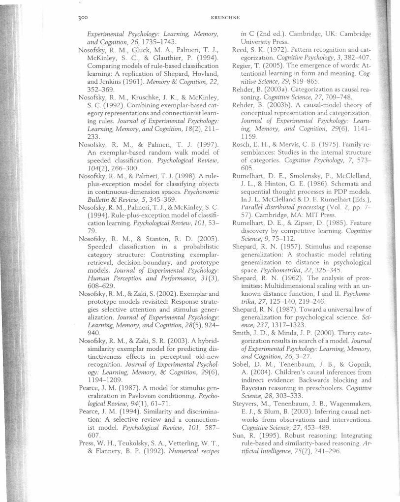
KRUSCHKE

Experimental Psychology: Learning, Memory, and Cognition, 26, 1735-1743.

Nosofsky, R. M., Gluck, M. A., Palmeri, T J., McKinley, S. c., & Glauthier, P. (1994) . Comparing models of rule-based classification learning: A replication of Shepard, Hovland, and Jenkins (1961). Memory & Cognition, 22, 352-369.

Nosofsky, R. M., Kruschke, J. K., & McKinley, S. C. (1992). Combining exemplar-based category representations and connectionist learning rules. Journal of Experimental Psychology: Learning, Memory, and Cognition, 18(2), 211-233.

Nosofsky, R. M., & Palmeri, T J. (1997). An exemplar-based random walk model of speeded classification. Psychological Review, 104(2), 266-300.

Nosofsky, R. M., & Palmeri, T J. (1998). A ruleplus-exception model for classifying objects in continuous-dimension spaces. Psychonomic Bulletin & Review, 5, 345-369.

Nosofsky, R. M., Palmeri, T J., & McKinley, S. C. (1994). Rule-plus-exception model of classification learning. Psychological Review, 101, 53-79.

Nosofsky, R. M., & Stanton, R. D . (2005). Speeded classification in a probabilistic category structure: Contrasting exemplarretrieval, decision-boundary, and prototype models. Journal of Experimental Psychology: Human Perception and Performance, 31 (3), 608-629.

Nosofsky, R. M., &Zaki, S. (2002). Exemplar and prototype models revisited: Response strategies selective attention and stimulus generalization. Journal of Experimental Psychology: Learning, Memory, and Cognition, 28(5), 924-940.

Nosofsky, R. M., & Zaki, S. R. (2003). A hybridsimilarity exemplar model for predicting distinctiveness effects in perceptual old-new recognition. Journal of Experimental Psychology: Learning, Memory, & Cognition, 29(6), 1194-1209.

Pearce, J. M. (1987) . A model for stimulus generalization in Pavlovian conditioning. Psychological Review, 94(1), 61-71.

Pearce, J. M. (1994). Similarity and discrimination: A selective review and a connectionist model. Psychological Review, 101, 587-607.

Press, W. H ., Teukolsky, S. A., Vetterling, W . T, & Flannery, B. P. (1992). Numerical recipes

in C (2nd ed.). Cambridge, UK: Cambridge University Press.

Reed, S. K. (1972). Pattern recognition and categorization. Cognitive Psychology, 3, 382-407.

Regier, T (2005) . The emergence of words: Attentionallearning in form and meaning. Cognitive Science, 29, 819-865.

Rehder, B. (2003a). Categorization as causal reasoning. Cognitive Science, 27, 709-748.

Rehder, B. (2003b). A causal-model theory of conceptual representation and categorization. Journal of Experimental Psychology: Learning, Memory, and Cognition, 29(6), 1141-1159.

Rosch, E. H., & Mervis, C. B. (1975). Family resemblances: Studies in the internal structure of categories. Cognitive Psychology, 7, 573-605.

Rumelhart, D . E., Smolensky, P., McClelland, J. L., & Hinton, G . E. (1986). Schemata and sequential thought processes in PDP models. In J. L. McClelland & D. E. Rumelhart (Eds .), Parallel distributed processing (Vol. 2, pp . 7-57). Cambridge, MA: MIT Press.

Rumelhart, D . E., & Zipser, D. (1985). Feature discovery by competitive learning. Cognitive Science, 9, 75-112.

Shepard, R. N. (1957). Stimulus and response generalization: A stochastic model relating generalization to distance in psychological space. Psychometrika, 22, 325-345.

Shepard, R. N. (1962). The analysis of proximities: Multidimensional scaling with an unknown distance function, I and II. Psychometrika, 27, 125-140,219-246.

Shepard, R. N . (1987) . Toward a universal law of generalization for psychological science. Science, 237,1317-1323 .

Smith, J. D ., & Minda, J. P. (2000). Thirty categorization results in search of a model. Journal of Experimental Psychology: Learning, Memory, and Cognition, 26, 3-27.

Sobel, D. M., Tenenbaum, J. B., & Gopnik, A. (2004). Children's causal inferences from indirect evidence: Backwards blocking and Bayesian reasoning in preschoolers. Cognitive Science, 28, 303-333.

Steyvers, M., Tenenbaum, J. B., Wagenmakers, E. J., & Blum, B. (2003) . Inferring causal networks from observations and interventions. Cognitive Science, 27, 453-489.

Sun, R. (1995). Robust reasoning: Integrating rule-based and Similarity-based reasoning. Artificial Intelligence, 75(2), 241-296.

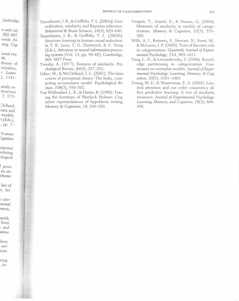
::ambridge

nand cat-382-407.

vords: Atling. Cog-

:ausal rea-48.

theory of orization. I: Learn), 1141-

amily restructure 7, 573-

::::lelland, nata and models.

t (Eds.), , pp. 7-

Feature ~ognitive

esponse relating ological

f proxan un

,chome-

[lawof :e. Sci-

y cate'oumal emory,

opnik, ; from g and ;nitive

akers, II nettions.

-ating 5. Ar-


Tenenbaum,J. B., & Griffiths, T L (2001 a). Generalization, similarity and Bayesian inference. Behavioral & Brain Sciences, 24(4), 629-640.

Tenenbaum, 1. B., & Griffiths, T L (2001 b). Structure learning in human causal induction. In T K. Leen, T G. Dietterich, & V. Tresp (Eds.), Advances in neural information processing systems (Vol. 13, pp. 59-65). Cambridge, MA: MIT Press.

Tversky, A. (1977). Features of Similarity. Psychological Review, 84(4), 327-352.

Usher, M., & McClelland, J. L (2001). The time course of perceptual choice: The leaky, competing accumulator model. Psychological Review, 108(3), 550-592.

Van Wallendael, L R., & Hastie, R. (1990). Tracing the footsteps of Sherlock Holmes: Cognitive representations of hypothesis testing. Memory & Cognition, 18, 240-250.

Verguts, T, Ameel, E., & Storms, G. (2004). Measures of similarity in models of categorization. Memory & Cognition, 32(3), 379-389.

Wills, A. J., Reimers, S., Stewart, N., Suret, M., & McLaren, L P. (2000). Tests of the ratio rule in categorization. Quarterly Journal of Experimental Psychology, 53A, 983-1011.

Yang, L-X., & Lewandowsky, S. (2004) . Knowledge partitioning in categorization: Constraints on exemplar models. Journal of Experimental Psychology: Learning, Memory, & Cognition, 30(5), 1045-1064.

Young, M. E., & Wasserman, E. A. (2002). limited attention and cue order consistency affect predictive learning: A test of similarity measures. Journal of Experimental Psychology: Learning, Memory, and Cognition, 28(3), 484-496.

Documents

Models of Categorization