Embed Size (px)
Citation preview

MODELS AND METRICS FOR
ENERGY-EFFICIENT COMPUTER SYSTEMS
A DISSERTATION
SUBMITTED TO THE DEPARTMENT OF ELECTRICAL
ENGINEERING
AND THE COMMITTEE ON GRADUATE STUDIES
OF STANFORD UNIVERSITY
IN PARTIAL FULFILLMENT OF THE REQUIREMENTS
FOR THE DEGREE OF
DOCTOR OF PHILOSOPHY
Suzanne Marion Rivoire
June 2008

© Copyright by Suzanne Marion Rivoire 2008
All Rights Reserved
ii

I certify that I have read this dissertation and that, in my opinion, it is fully
adequate in scope and quality as a dissertation for the degree of Doctor of
Philosophy.
(Christoforos Kozyrakis) Principal Adviser
I certify that I have read this dissertation and that, in my opinion, it is fully
adequate in scope and quality as a dissertation for the degree of Doctor of
Philosophy.
(Oyekunle Olukotun)
I certify that I have read this dissertation and that, in my opinion, it is fully
adequate in scope and quality as a dissertation for the degree of Doctor of
Philosophy.
(Parthasarathy Ranganathan)
Approved for the University Committee on Graduate Studies.
iii

Abstract
Energy e!ciency is an important concern in computer systems from small handheld de-
vices to large data centers and supercomputers. Improving energy e!ciency requires met-
rics and models: metrics to assess designs and identify promising energy-e!cient technolo-
gies, and models to understand the e"ects of resource utilization decisions on power con-
sumption. To facilitate energy-e!ciency improvements, this dissertation presents Joule-
Sort, the first completely specified full-system energy-e!ciency benchmark; and Mantis, a
generic and portable approach to real-time, full-system power modeling.
JouleSort was the first full-system energy-e!ciency benchmark with fully specified
workload, metric, and rules. This dissertation describes the benchmark design, highlight-
ing the challenges and pitfalls of energy-e!ciency benchmarking that distinguish it from
benchmarking pure performance. It also describes the design of the machine with the high-
est known JouleSort score. This machine, consisting of a commodity mobile CPU and 13
laptop drives connected by server-style I/O interfaces, di"ers greatly from today’s commer-
cially available servers.
Mantis generates full-system power models by correlating AC power measurements
with software utilization metrics. This dissertation will evaluate several di"erent families
of Mantis-generated models on several computer systems with widely varying components
and power footprints, identifying models that are both highly accurate and highly portable.
This evaluation demonstrates the trade-o" between simplicity and accuracy, and it also
iv

shows the limitations of previously proposed models based solely on OS-reported com-
ponent utilization. The simplicity of this black-box approach makes it a useful tool for
power-aware scheduling and analysis.
v

Acknowledgments
I am grateful to many people for their contributions to this dissertation and to the quality of
my life while I worked on it.
First, it has been an honor to work with Christos Kozyrakis, my advisor. I am pro-
foundly grateful to him for his perceptive, patient, and unselfish mentoring over the last six
years. He has been an unfailing source of honest and supportive advice in my research and
in my career, and because of him, I have become a much more competent and confident
scholar and teacher.
I am also deeply thankful to Partha Ranganathan, my mentor at HP Labs. Partha has
been amazingly generous in providing me with professional opportunities, starting with the
opportunity to work on the research described in this dissertation. He has also been a wise
and compassionate mentor whose guidance and support have been indispensable.
I am also grateful to Kunle Olukotun for serving on my reading committee and to
Dwight Nishimura for chairing the examining committee for my defense. Kunle’s feedback
on my work and help during the job search process have been very beneficial to me.
This research would not have been possible without my collaborators and co-authors.
Mehul Shah and I worked closely together to bring his idea of an energy-e!ciency ex-
tension of the Sort Benchmark to fruition. I am grateful to him for his patience and his
willingness to help with every aspect of the work. I was also fortunate to work with two
dedicated, talented, and highly skilled undergraduate students: Justin Meza, who extended
my work in designing energy-e!cient sorting systems, and Dimitris Economou, whose
vi

work paved the way for the modeling study in this thesis and who contributed to the study
of the Itanium machine discussed in Chapter 7. I also greatly appreciate the outside feed-
back from Luiz Barroso, Wolf-Dietrich Weber, Taliver Heath, Feng Zhao, Kim Shearer,
Bill Bolosky, Naga Govindaraju, Chris Reummler, and Jim Gray, and from the participants
at UC-Berkeley’s RAD Lab retreats.
The work described in Chapter 4 relied on Ordinal Technology’s Nsort software, and I
am grateful to Ordinal’s Chris Nyberg and Charles Koester for their generosity with their
time and support. Similarly, the work described in Chapters 6 and 7 relied on software
written by Justin Moore and by Stephane Eranian, for whose assistance I am also grateful.
Jacob Leverich provided valuable contributions to several aspects of this research. First,
he was indispensable in configuring the hardware and software of the CoolSort machine.
Second, he helped to instrument and configure one of the machines used to validate my
power models. Third, he was an excellent system administrator for our research group, a
job that I am also thankful to him for taking o" of my hands. Fourth, hook ’em Horns!
This work also benefited from the administrative and technical assistance of Teresa
Lynn, Charlie Orgish, and Joe Little at Stanford; and Annabelle Eseo, Hernan La!tte,
Craig Soules, Malena Mesarina, Christina Solorzano, and Rowena Fernandez at HP. Teresa
in particular showed great forbearance during the process of ordering the CoolSort machine
piece by piece.
Funding for my doctoral work was provided by several sources. I am grateful to the
anonymous donor of my Stanford Graduate Fellowship and to the National Science Foun-
dation for their graduate fellowship. My initial research was done with the support of Cray,
and I am grateful to Cray’s Steve Scott for his mentoring; he gave me enough independence
to build my confidence as a researcher, while always being available for advice and feed-
back. My subsequent research was supported by HP Labs, for which I am thankful to John
Sontag as well as Partha and Mehul; and by Google.
vii

On a more personal level, the support of more senior graduate students has been es-
sential to surviving in Stanford’s huge electrical engineering department. From the time I
first set foot on the Stanford campus as a prospective graduate student, Kerri Cahoy took
me under her wing and introduced me to EE students outside the Computer Systems Lab.
Later, when I started doing research, the advice and support of senior students helped me
find my way. Bennett Wilburn, Kelly Shaw, John Davis, and Mattan Erez were particularly
generous and helpful.
My fellow graduate students at Stanford and in the computer architecture community
have made my graduate school years more productive and enjoyable. In particular, Allison
Holloway has been there for me from the introductory electrical engineering course in
the first semester of our freshman year of college all the way through the Ph.D. process.
Additionally, Jayanth Gummaraju, Nju Njoroge, Joel Coburn, Dan Finkelstein, and Nidhi
Aggarwal have become good friends and colleagues. Finally, I appreciate the camaraderie
and support of my current and former groupmates: Varun Malhotra, Rebecca Schultz (who
was also a dedicated research collaborator), Austen McDonald, Chi Cao Minh, Sewook
Wee, Woongki Baek, JaeWoong Chung, Michael Dalton, Hari Kannan, and Jacob Leverich.
During graduate school, I have been fortunate to become involved in several IEEE com-
mittees. It has been rewarding and inspirational to work with such a diverse and passionate
group of engineers, and it has taught me a great deal about my profession. In particular,
I have worked on IEEE Potentials with Phil Wilsey, Kim Tracy, and George Zobrist since
2002, and they have been generous both in providing professional opportunities and in
giving academic and career guidance.
Finally, I am also grateful to all my friends and my entire family for the opportunities
and support they provided me. My mother, Elizabeth Rivoire Lee, has been a loving and
supportive presence in my life, and learned early not to ask when the Ph.D. would be
finished. My late father, Thomas Alexis Rivoire, spent years persuading me that I could
and should pursue a technical career, and I know he would be proud of where I am today. I
viii

also owe a special debt to the other engineers in the family: my grandfather, Bernard Rider,
whose love of math and problem-solving is contagious, and my sister, Kelley Rivoire, who
is a great friend with interesting perspectives on our field. The past few years have brought
wonderful new additions to my family, including my stepfather, Bob Lee, and my husband,
Grant Gavranovic. I am very grateful to Grant for the many years of friendship, love, and
support we have shared. He has enriched my life and made every day happier.
ix

Contents
Abstract iv
Acknowledgments vi
1 Introduction 1
1.1 Motivation . . . . . . . . . . . . . . . . . . . . . . . . . . . . . . . . . . . 2
1.2 Contributions . . . . . . . . . . . . . . . . . . . . . . . . . . . . . . . . . 3
1.3 Dissertation Outline . . . . . . . . . . . . . . . . . . . . . . . . . . . . . . 4
2 Benchmarking Energy E!ciency 6
2.1 Benchmarking Challenges . . . . . . . . . . . . . . . . . . . . . . . . . . 7
2.2 Energy-E!ciency Benchmark Goals . . . . . . . . . . . . . . . . . . . . . 8
2.3 Current Energy-E!ciency Metrics . . . . . . . . . . . . . . . . . . . . . . 10
2.3.1 Component-level Benchmarks and Metrics . . . . . . . . . . . . . 10
2.3.2 System-level Benchmarks and Metrics . . . . . . . . . . . . . . . . 12
2.3.3 Data Center-level Benchmarks and Metrics . . . . . . . . . . . . . 14
2.3.4 Summary . . . . . . . . . . . . . . . . . . . . . . . . . . . . . . . 15
3 The Joulesort Benchmark Definition 16
3.1 Workload . . . . . . . . . . . . . . . . . . . . . . . . . . . . . . . . . . . 17
3.2 Metric . . . . . . . . . . . . . . . . . . . . . . . . . . . . . . . . . . . . . 19
x

3.2.1 Fixed Energy Budget . . . . . . . . . . . . . . . . . . . . . . . . . 19
3.2.2 Fixed Time Budget . . . . . . . . . . . . . . . . . . . . . . . . . . 20
3.2.3 Fixed Input Size . . . . . . . . . . . . . . . . . . . . . . . . . . . 23
3.3 Benchmark Categories . . . . . . . . . . . . . . . . . . . . . . . . . . . . 24
3.4 Measuring Energy . . . . . . . . . . . . . . . . . . . . . . . . . . . . . . . 25
3.4.1 System Boundaries . . . . . . . . . . . . . . . . . . . . . . . . . . 25
3.4.2 Ambient Environment . . . . . . . . . . . . . . . . . . . . . . . . 26
3.4.3 Measurement and Instrumentation . . . . . . . . . . . . . . . . . . 26
3.5 Summary . . . . . . . . . . . . . . . . . . . . . . . . . . . . . . . . . . . 27
4 Designing Energy-E!cient Computer Systems 29
4.1 Energy E!ciency of Past Sort Benchmark Winners . . . . . . . . . . . . . 30
4.1.1 Methodology . . . . . . . . . . . . . . . . . . . . . . . . . . . . . 30
4.1.2 Analysis . . . . . . . . . . . . . . . . . . . . . . . . . . . . . . . 32
4.2 Evaluation of Commodity Systems . . . . . . . . . . . . . . . . . . . . . . 35
4.2.1 Unbalanced Systems . . . . . . . . . . . . . . . . . . . . . . . . . 35
4.2.2 Balanced Server . . . . . . . . . . . . . . . . . . . . . . . . . . . 38
4.2.3 Summary . . . . . . . . . . . . . . . . . . . . . . . . . . . . . . . 40
4.3 Design of the JouleSort Winner . . . . . . . . . . . . . . . . . . . . . . . . 40
4.3.1 Details of Winning Configuration . . . . . . . . . . . . . . . . . . 41
4.3.2 Varying Hardware Configuration . . . . . . . . . . . . . . . . . . . 43
4.3.3 Varying Software Configuration . . . . . . . . . . . . . . . . . . . 51
4.3.4 CPU and I/O Dynamic Power Variation . . . . . . . . . . . . . . . 52
4.3.5 Summary . . . . . . . . . . . . . . . . . . . . . . . . . . . . . . . 53
4.4 Other Energy-E!ciency Metrics . . . . . . . . . . . . . . . . . . . . . . . 53
4.5 Conclusions . . . . . . . . . . . . . . . . . . . . . . . . . . . . . . . . . . 63
xi

5 Power Modeling Background 65
5.1 Power Modeling Goals . . . . . . . . . . . . . . . . . . . . . . . . . . . . 66
5.2 Power Modeling Approaches . . . . . . . . . . . . . . . . . . . . . . . . . 67
5.2.1 Simulation-based Power Models . . . . . . . . . . . . . . . . . . . 68
5.2.2 Detailed Analytical Power Models . . . . . . . . . . . . . . . . . . 70
5.2.3 High-level Black-box Power Models . . . . . . . . . . . . . . . . . 72
6 The Mantis Power Modeling Methodology 76
6.1 Overview of Model Development and Evaluation . . . . . . . . . . . . . . 77
6.2 Calibration Process . . . . . . . . . . . . . . . . . . . . . . . . . . . . . . 79
6.2.1 Calibration Software Suite . . . . . . . . . . . . . . . . . . . . . . 80
6.2.2 Portability and Limitations . . . . . . . . . . . . . . . . . . . . . . 81
6.3 Model Inputs . . . . . . . . . . . . . . . . . . . . . . . . . . . . . . . . . 82
6.4 Models Studied . . . . . . . . . . . . . . . . . . . . . . . . . . . . . . . . 84
6.5 Evaluation Process . . . . . . . . . . . . . . . . . . . . . . . . . . . . . . 85
6.5.1 Introduction . . . . . . . . . . . . . . . . . . . . . . . . . . . . . . 85
6.5.2 Machines . . . . . . . . . . . . . . . . . . . . . . . . . . . . . . . 86
6.5.3 Benchmarks . . . . . . . . . . . . . . . . . . . . . . . . . . . . . . 89
7 Power Modeling Evaluation 92
7.1 Overall Results . . . . . . . . . . . . . . . . . . . . . . . . . . . . . . . . 93
7.2 Xeon Server Power Models . . . . . . . . . . . . . . . . . . . . . . . . . . 102
7.3 Itanium Server Power Models . . . . . . . . . . . . . . . . . . . . . . . . 108
7.4 CoolSort-13 Power Models . . . . . . . . . . . . . . . . . . . . . . . . . . 113
7.4.1 CoolSort-13, Highest Clock Frequency . . . . . . . . . . . . . . . 113
7.4.2 CoolSort-13, Lowest Clock Frequency . . . . . . . . . . . . . . . . 117
7.5 CoolSort-1 Power Models . . . . . . . . . . . . . . . . . . . . . . . . . . 118
7.5.1 CoolSort-1, Highest Clock Frequency . . . . . . . . . . . . . . . . 121
xii

7.5.2 CoolSort-1, Lowest Clock Frequency . . . . . . . . . . . . . . . . 125
7.6 Laptop Power Models . . . . . . . . . . . . . . . . . . . . . . . . . . . . . 126
7.6.1 Laptop, Highest Clock Frequency . . . . . . . . . . . . . . . . . . 129
7.6.2 Laptop, Lowest Clock Frequency . . . . . . . . . . . . . . . . . . 133
7.7 Conclusions . . . . . . . . . . . . . . . . . . . . . . . . . . . . . . . . . . 134
8 Conclusions 139
8.1 Future Work . . . . . . . . . . . . . . . . . . . . . . . . . . . . . . . . . . 141
Bibliography 144
xiii

List of Tables
2.1 Summary of the target domains of di"erent energy-e!ciency benchmarks
and metrics. . . . . . . . . . . . . . . . . . . . . . . . . . . . . . . . . . . 11
2.2 Summary of the specifications of di"erent energy-e!ciency benchmarks
and metrics. . . . . . . . . . . . . . . . . . . . . . . . . . . . . . . . . . . 11
3.1 Summary of sort benchmarks. . . . . . . . . . . . . . . . . . . . . . . . . 18
4.1 Estimated yearly improvement in pure performance (SRecs/sec), price-
performance (SRecs/$), and energy e!ciency (SRecs/J) of past Sort
Benchmark winners. Performance sorts include MinuteSort, Terabyte
Sort, and Datamation Sort. . . . . . . . . . . . . . . . . . . . . . . . . . . 34
4.2 Summary of commodity systems for which the JouleSort rating was exper-
imentally measured. . . . . . . . . . . . . . . . . . . . . . . . . . . . . . . 35
4.3 Specifications of the unbalanced commodity systems listed in Table 4.2. . . 36
4.4 JouleSort benchmark scores of unbalanced commodity systems. . . . . . . 36
4.5 Specifications of the balanced fileserver. . . . . . . . . . . . . . . . . . . . 39
4.6 Components of the CoolSort machine and their retail prices at the time of
purchase. . . . . . . . . . . . . . . . . . . . . . . . . . . . . . . . . . . . 41
4.7 Power and performance of winning JouleSort systems. . . . . . . . . . . . 42
xiv

4.8 Detailed utilization information for winning JouleSort systems, including
the number of sorted records, the sorting bandwidths and CPU utilization,
and the power factor (PF). . . . . . . . . . . . . . . . . . . . . . . . . . . 42
4.9 CoolSort configurations with varying numbers of disks. For each number
of disks shown in the left-hand column, the next three columns show the
number of disks attached to the 4-disk controller, the 8-disk controller, and
the motherboard, respectively. A controller is removed from the system if
no disks are attached to it. . . . . . . . . . . . . . . . . . . . . . . . . . . . 44
4.10 Low-power machines benchmarked by Meza et al. [45]. . . . . . . . . . . . 54
6.1 Summary of machines used to evaluate Mantis-generated models. . . . . . 86
6.2 Xeon server components. . . . . . . . . . . . . . . . . . . . . . . . . . . . 87
6.3 Itanium server components. . . . . . . . . . . . . . . . . . . . . . . . . . . 87
6.4 CoolSort components for modeling study. . . . . . . . . . . . . . . . . . . 88
6.5 Laptop components. . . . . . . . . . . . . . . . . . . . . . . . . . . . . . . 88
6.6 Selected properties of Mantis evaluation machines. . . . . . . . . . . . . . 89
6.7 Descriptions of benchmarks selected to evaluate Mantis models. . . . . . . 89
6.8 Component utilizations of Mantis evaluation benchmarks. . . . . . . . . . . 91
7.1 Model calibration results for the Xeon server. . . . . . . . . . . . . . . . . 105
7.2 Model calibration results for the Itanium server. . . . . . . . . . . . . . . . 109
7.3 Model calibration results for CoolSort-13 at its highest frequency. . . . . . 114
7.4 Model calibration results for CoolSort-13 at its lowest frequency. . . . . . . 118
7.5 Model calibration results for CoolSort-1 at its highest frequency. . . . . . . 122
7.6 Model calibration results for CoolSort-1 at its lowest frequency. . . . . . . 126
7.7 Model calibration results for the laptop at its highest frequency. . . . . . . . 131
7.8 Model calibration results for the laptop at its lowest frequency. . . . . . . . 134
xv
List of Figures
3.1 The measured energy e!ciency of the current JouleSort-winning system at
varying input sizes. . . . . . . . . . . . . . . . . . . . . . . . . . . . . . . 22
4.1 Estimated energy e!ciency of previous winners of sort benchmarks. . . . . 32
4.2 Variation of performance and price-performance with the number of disks
in the CoolSort system. . . . . . . . . . . . . . . . . . . . . . . . . . . . . 45
4.3 Variation of power consumption with the number of disks in the CoolSort
system. . . . . . . . . . . . . . . . . . . . . . . . . . . . . . . . . . . . . 46
4.4 Variation of energy e!ciency with the number of disks in the CoolSort
system. . . . . . . . . . . . . . . . . . . . . . . . . . . . . . . . . . . . . 48
4.5 Variation of average power and energy e!ciency with CPU frequency and
filesystem for a 10 GB sort on CoolSort. . . . . . . . . . . . . . . . . . . . 50
4.6 PennySort scores of energy-aware systems and previous PennySort bench-
mark winners, normalized to the lowest-scoring system. . . . . . . . . . . . 55
4.7 JouleSort scores of energy-aware systems and previous PennySort, Min-
uteSort, and Terabyte Sort benchmark winners, normalized to the lowest-
scoring system. . . . . . . . . . . . . . . . . . . . . . . . . . . . . . . . . 56
4.8 Records sorted per Joule per dollar of purchase price of energy-aware sys-
tems and previous PennySort winners, normalized to the lowest-scoring
system. . . . . . . . . . . . . . . . . . . . . . . . . . . . . . . . . . . . . 57
xvi

4.9 Product of JouleSort and PennySort scores of energy-aware systems and
previous PennySort winners, on a logarithmic scale, normalized to the
lowest-scoring system. . . . . . . . . . . . . . . . . . . . . . . . . . . . . 58
4.10 Reciprocal of energy-delay product of energy-aware systems and previous
sort benchmark winners, on a logarithmic scale, normalized to the lowest-
scoring system. . . . . . . . . . . . . . . . . . . . . . . . . . . . . . . . . 60
4.11 Performance-TCO ratio for energy-aware systems, normalized to the
lowest-scoring system. . . . . . . . . . . . . . . . . . . . . . . . . . . . . 61
6.1 Overview of Mantis model generation and use. . . . . . . . . . . . . . . . 78
6.2 Mantis instrumentation setup. . . . . . . . . . . . . . . . . . . . . . . . . . 79
7.1 Overall mean absolute error for Mantis-generated models over all bench-
marks and machine configurations. . . . . . . . . . . . . . . . . . . . . . . 94
7.2 Overall 90th percentile absolute error for Mantis-generated models over all
benchmarks and machine configurations. . . . . . . . . . . . . . . . . . . . 95
7.3 Best case for the empirical CPU-utilization-based model: CPU-intensive
benchmarks on Xeon server. . . . . . . . . . . . . . . . . . . . . . . . . . 96
7.4 Power predicted by the empirical CPU-utilization-based model versus CPU
utilization for the Xeon server. . . . . . . . . . . . . . . . . . . . . . . . . 97
7.5 Measured power versus CPU utilization for the Xeon server during the cal-
ibration suite. Note that memory and disk utilization also varied over this
data. . . . . . . . . . . . . . . . . . . . . . . . . . . . . . . . . . . . . . . 98
7.6 Best case for the CPU- and disk-utilization-based model: Selected bench-
marks on CoolSort-13 at the highest frequency. . . . . . . . . . . . . . . . 100
7.7 Power predicted by the CPU-utilization-based models and the CPU and
disk-utilization-based model versus CPU utilization on CoolSort-13 at its
highest frequency. Disk utilization is assumed to be 0. . . . . . . . . . . . . 101
xvii
7.8 Best case for the performance-counter-based model: Selected benchmarks
on the Xeon server and on CoolSort-13 at the highest frequency. . . . . . . 103
7.9 Mean absolute percentage error of the Mantis-generated models on the
Xeon server. . . . . . . . . . . . . . . . . . . . . . . . . . . . . . . . . . . 106
7.10 90th percentile absolute percentage error of the Mantis-generated models
on the Xeon server. . . . . . . . . . . . . . . . . . . . . . . . . . . . . . . 107
7.11 Mean absolute percentage error of the Mantis-generated models on the Ita-
nium server. . . . . . . . . . . . . . . . . . . . . . . . . . . . . . . . . . . 111
7.12 90th percentile absolute percentage error of the Mantis-generated models
on the Itanium server. . . . . . . . . . . . . . . . . . . . . . . . . . . . . . 112
7.13 Mean absolute percentage error of the Mantis-generated models on
CoolSort-13 at its highest frequency. . . . . . . . . . . . . . . . . . . . . . 115
7.14 90th percentile absolute percentage error of the Mantis-generated models
on CoolSort-13 at its highest frequency. . . . . . . . . . . . . . . . . . . . 116
7.15 Mean absolute percentage error of the Mantis-generated models on
CoolSort-13 at its lowest frequency. . . . . . . . . . . . . . . . . . . . . . 119
7.16 90th percentile absolute percentage error of the Mantis-generated models
on CoolSort-13 at its lowest frequency. . . . . . . . . . . . . . . . . . . . . 120
7.17 Mean absolute percentage error of the Mantis-generated models on
CoolSort-1 at its highest frequency. . . . . . . . . . . . . . . . . . . . . . . 123
7.18 90th percentile absolute percentage error of the Mantis-generated models
on CoolSort-1 at its highest frequency. . . . . . . . . . . . . . . . . . . . . 124
7.19 Mean absolute percentage error of the Mantis-generated models on
CoolSort-1 at its lowest frequency. . . . . . . . . . . . . . . . . . . . . . . 127
7.20 90th percentile absolute percentage error of the Mantis-generated models
on CoolSort-1 at its lowest frequency. . . . . . . . . . . . . . . . . . . . . 128
xviii
7.21 Mean absolute percentage error of the Mantis-generated models on the lap-
top at its highest frequency. . . . . . . . . . . . . . . . . . . . . . . . . . . 131
7.22 90th percentile absolute percentage error of the Mantis-generated models
on the laptop at its highest frequency. . . . . . . . . . . . . . . . . . . . . . 132
7.23 Mean absolute percentage error of the Mantis-generated models on the lap-
top at its lowest frequency. . . . . . . . . . . . . . . . . . . . . . . . . . . 135
7.24 90th percentile absolute percentage error of the Mantis-generated models
on the laptop at its lowest frequency. . . . . . . . . . . . . . . . . . . . . . 136
xix

Chapter 1
Introduction
1

CHAPTER 1. INTRODUCTION 2
1.1 Motivation
In contexts ranging from large-scale data centers to mobile devices, energy use is an im-
portant concern. In data centers, according to the United States Environmental Protection
Agency, power consumption in the United States doubled between 2000 and 2006, and
will double again in the next five years [74]. Server power consumption not only directly
a"ects a data center’s energy costs, but also necessitates the purchase and operation of cool-
ing equipment, which can consume one-half to one Watt for every Watt of power consumed
by the computing equipment.
In addition, energy use has implications for reliability, density, and scalability. As data
centers house more servers and consume more energy, removing heat from the data cen-
ter becomes increasingly di!cult [49]. Since the reliability of servers and disks decreases
at high temperatures, the power consumption of servers and other components limits the
achievable density of data centers, which in turn limits their scalability. Furthermore, en-
ergy use in data centers is starting to prompt environmental concerns of pollution and ex-
cessive load placed on local utilities [51]. These concerns are su!ciently severe that large
companies are starting to build data centers near electric plants in cold-weather environ-
ments [42].
In mobile devices, battery capacity and energy use directly a"ect usability. Battery
capacity determines how long devices last, constrains form factors, and limits functionality.
Since battery capacity is limited and improving slowly, device architects have concentrated
on extracting greater e!ciency from the individual underlying components, such as the
processor, the display, and the wireless subsystems.
To facilitate energy-e!ciency optimizations, we need metrics and models. Metrics help
define energy e!ciency, giving a basis on which to compare designs and a way to identify
promising energy-e!cient technologies. Models show the relationship between resource

CHAPTER 1. INTRODUCTION 3
utilization and power consumption, which allows data center scheduling algorithms or in-
dividual users to tailor their usage to maximize energy e!ciency.
To address these challenges, this dissertation presents the JouleSort energy-e!ciency
benchmark and the Mantis approach to high-level power modeling.
1.2 Contributions
The main contributions of this dissertation are the following:
• It presents the specification for JouleSort, the first completely specified, full-system
energy-e!ciency benchmark to be proposed. It describes the benchmark workload,
metric, and rules, highlighting the unique challenges of designing a benchmark for
energy e!ciency.
• It presents the energy-e!cient CoolSort system, the machine with the highest known
JouleSort benchmark score, which is over 3.5 times more energy-e!cient than pre-
vious systems. CoolSort consists of a high-end mobile processor connected to 13
SATA laptop disks. This unusual configuration suggests a promising new approach
to energy-e!cient hardware design. The CoolSort design and the JouleSort specifi-
cation were originally presented in [57] and [58].
• It presents a method of high-level, full-system power modeling that uses a linear com-
bination of OS utilization metrics and hardware performance counters, and demon-
strates that this model accurately predicts power consumption over a very wide range
of hardware configurations and software workloads. This model was originally pre-
sented in [14].
• It provides a detailed evaluation of several previously proposed high-level power
models, noting the types of systems to which each model is best suited and the trade-
o"s between model complexity and prediction accuracy. This analysis shows that the

CHAPTER 1. INTRODUCTION 4
modeling approach we proposed, based on OS utilization metrics and performance
counters, is the most accurate type of model across the machines and workloads
tested. It is particularly useful for machines whose dynamic power consumption
is not dominated by the CPU and for machines with aggressively power-managed
CPUs, two classes of systems that are increasingly prevalent.
1.3 Dissertation Outline
Chapters 2 through 4 present the JouleSort energy-e!ciency benchmark. Chapter 2 pro-
vides background on the problem of benchmarking for energy e!ciency, examining the
goals of an energy-e!ciency benchmark and the limitations of previous approaches.
Chapter 3 presents the specification for the JouleSort benchmark, which was the first
completely specified, full-system energy-e!ciency benchmark to be proposed. It explains
the JouleSort workload, metric, and rules, as well as the challenges and pitfalls of designing
a fair benchmark for energy e!ciency.
Chapter 4 presents the CoolSort machine, an energy-e!cient sorting system that
achieves the highest known JouleSort score. It also evaluates the JouleSort benchmark
scores of a variety of other systems, including the best-performing and most cost-e!cient
winners of previous sort benchmarks, as well as commodity machines from a variety of
system classes. Finally, it compares the JouleSort metric to metrics using other combi-
nations of performance, cost, and power. Di"erent combinations of these metrics favor
di"erent system classes, but the high score of the CoolSort machine is not highly sensitive
to changes in the metric.
Chapters 5 through 7 describe the Mantis approach to portable and general high-level
full-system power modeling. Chapter 5 defines the goals of the Mantis approach and ex-
amines previous approaches to power modeling at the architectural level and higher, from

CHAPTER 1. INTRODUCTION 5
detailed simulation-based power models to very simple high-level models based on a sin-
gle metric. It compares the accuracy, generality, and level of detail of these previously
proposed models, and assesses their suitability with respect to the Mantis goals.
Chapter 6 explains the Mantis model generation and evaluation methodology. It de-
scribes the models themselves as well as the process of generating the models, including
a detailed discussion of the software calibration suite and the hardware infrastructure. It
also details the hardware and software configurations on which the models are evaluated in
Chapter 7.
Chapter 7 presents the results of generating and evaluating the Mantis models on a
wide range of machines. In general, the model that we proposed, which uses a linear com-
bination of CPU performance counters and OS-reported component utilizations, is most
accurate. We show the strengths and limitations of each model and make a case that OS-
reported CPU utilization alone will be an increasingly less useful proxy for system-level
power consumption in the future. Finally, Chapter 8 concludes the dissertation and suggests
directions for future work.

Chapter 2
Benchmarking Energy E!ciency
6

CHAPTER 2. BENCHMARKING ENERGY EFFICIENCY 7
Energy e!ciency is a pressing concern in computer systems, from mobile devices to
data centers. Energy-conscious users, as well as computer manufacturers and researchers,
need to be able to assess and compare the energy e!ciency of computer systems in order to
make purchasing decisions or to identify promising technologies. Well-defined benchmarks
are needed to provide standardized and fair comparisons of computers’ energy e!ciency.
To this end, this thesis presents the JouleSort energy-e!ciency benchmark in Chapter 3.
This chapter lays the groundwork by explaining the challenges and complexities of energy-
e!ciency benchmarking, outlining the goals of the JouleSort benchmark, and describing
the goals and limitations of other energy-e!ciency benchmarks and metrics that have been
proposed.
2.1 Benchmarking Challenges
A complete benchmark specifies three things: a workload to run, which should represent
some real-world task of interest; a metric or “score” to compare di"erent systems; and
operational rules to ensure that the benchmark runs under realistic conditions. Creating
a benchmark for energy e!ciency shares some challenges with creating any benchmark.
There is the question of what to benchmark, e.g. components, single machines, or data cen-
ters. There is also the question of workload choice, which e"ectively also determines the
class of machines to which the benchmark can be applied; for example, a supercomputing
benchmark probably could not run on handheld devices, and would not be a representative
workload if it could. Benchmarks exist for almost every conceivable class of workload and
for every class of machine, from small embedded processors [15] to large clusters [72] and
supercomputers [54].
The benchmark metric must also be determined. Even when the goal is to measure pure
performance, the decision of whether to use a metric based on the time to execute a fixed-
size workload or the throughput in a fixed amount of time can bias the metric toward certain

CHAPTER 2. BENCHMARKING ENERGY EFFICIENCY 8
types of machines or exclude them entirely. When the goal is to balance performance with
another concern, such as cost, the question of how to weigh and combine the two metrics
in the final benchmark score adds another element of complexity.
Finally, the benchmark specification must include rules to ensure that the benchmark
runs under fair and realistic conditions. For performance-oriented benchmarks, these rules
often constrain the types of compiler optimizations that can be applied to the benchmark
source code in order to preclude benchmark-specific compiler optimizations of dubious
general correctness. The rules may also constrain the type of hardware, operating system,
or file system on which the benchmark is run.
Benchmarking energy e!ciency presents some unique challenges. The choice of work-
load is complicated by the fact that the desired operating point(s) of the system must be
identified; in particular, since lightly utilized systems are currently highly ine!cient [5],
benchmark designers may want to target this operating point. The choice of metric also
becomes more complex, since it must resolve the question of how to weigh performance
against power consumption. However, the benchmark rules are the largest source of in-
creased complexity. First, the definition of the system and its environment becomes more
complex. The ambient temperature around the system a"ects its power consumption, so
benchmark designers may want to regulate it. They also must decide whether or not to
include the cooling systems of both the machine and the building housing it, a significant
decision since cooling can consume up to one Watt for each Watt of power consumed by the
computing equipment [50]. Additionally, energy-e!ciency benchmarks require standards
to govern the accuracy and sampling rate of the power and temperature instrumentation.
2.2 Energy-E!ciency Benchmark Goals
The JouleSort benchmark was created with the goal of providing a fully specified energy-
e!ciency benchmark that was meaningful and broadly applicable in order to identify trends

CHAPTER 2. BENCHMARKING ENERGY EFFICIENCY 9
and inspire improvements in energy e!ciency. This section describes the design criteria
that the JouleSort specification seeks to balance.
Power-performance trade-o": The benchmark’s metric should capture a system’s per-
formance as well as some measure of power use. Peak or average power would be an
impractical metric, since neither includes a measurement of performance; the benchmark
should not reward a system that consumes almost no power and completes almost no work.
Two reasonable alternatives for the metric are energy, which is the product of execution
time and power; and the energy-delay product. The former metric weighs performance and
power equally, while the latter places more emphasis on performance. Since many bench-
marks already emphasize performance, we chose to use energy as the metric in order to
draw attention to power consumption.
Peak e!ciency: A benchmark can measure systems at their most energy-e!cient oper-
ating point, which corresponds to peak utilization for most computer systems [5], or it can
explicitly specify one or more di"erent operating points, as SPECpower ssj [68] does. For
simplicity of benchmarking and clarity of the benchmark score, our benchmark does not
specify an operating point and therefore measures peak energy e!ciency, giving an upper
bound on the work that can be done for a given power consumption. This operating point
influences design and provisioning constraints for data centers as well as mobile devices.
Furthermore, peak utilization is the most common operating point in some computing do-
mains, such as enterprise environments that use server consolidation to improve energy
e!ciency, as well as scientific computing.
Holistic and Balanced: A single component cannot accurately reflect the overall per-
formance and power characteristics of a system. Therefore, the workload should exercise
all core components and stress them roughly equally. The benchmark metric should incor-
porate the energy used by all core components.
Inclusive and Portable: The benchmark should be able to assess the energy e!cien-
cies of a wide variety of systems: PDAs, laptops, desktops, servers, clusters, and so on.

CHAPTER 2. BENCHMARKING ENERGY EFFICIENCY 10
It should be as unbiased as possible among architectures and system classes. Moreover,
the benchmark’s workload should be implementable and meaningful across all of these
platforms.
History-proof: In order to track improvements over generations of systems and iden-
tify promising new technologies, the benchmark specification should remain meaningful as
hardware and software technologies evolve, and it should allow comparisons across di"er-
ent generations of systems.
Representative: The benchmark’s workload should represent an important class of
workloads for the systems being benchmarked.
Simple: The benchmark should be as simple as possible to set up and administer, and
the score should be easy to understand.
The next section evaluates current energy-e!ciency benchmarks in light of these goals.
2.3 Current Energy-E!ciency Metrics
An ideal benchmark for energy e!ciency would consist of a universally relevant workload
that is portable to any computing device; a metric that balances power and performance in
a universally appropriate way; and rules that are impossible to circumvent and that provide
fair comparisons across every class of machine. This ideal is impossible to achieve in prac-
tice, so proposed metrics have specialized in di"erent classes of workloads and systems.
This section describes previously proposed energy-e!ciency benchmarks and metrics. Ta-
ble 2.1 shows the target system classes of these metrics, and Table 2.2 summarizes their
specifications.
2.3.1 Component-level Benchmarks and Metrics
At the processor level, Gonzalez and Horowitz argued in 1996 that the energy-delay product
was the appropriate metric for comparing two designs [20]. They observed that a chip’s

CHAPTER 2. BENCHMARKING ENERGY EFFICIENCY 11
Benchmark Level DomainEnergyBench Processor EmbeddedSWaP System(s) EnterpriseEnergy Star certification System Mobile, desktop, enterpriseSPECpower ssj System EnterpriseCompute Power E!ciency Data center EnterpriseGreen Grid metrics Data center Enterprise
Table 2.1: Summary of the target domains of di"erent energy-e!ciency benchmarks andmetrics.
Benchmark Workload MetricSWaP Unspecified Performance/(Space !Watts)EnergyBench EEMBC benchmarks Throughput/JouleEnergy Star: Sleep, idle, standby, Certify if “typical” powerworkstations Linpack, SPECviewperf < 35% of max. powerEnergy Star: Sleep, idle, Certify if each mode’sother systems standby modes power < predefined thresholdSPECpower ssj Server-side Java Operations/Watt
under varying loads averaged over all loadsGreen Grid DCD Unspecified Equipment power / floor
area (kW/ f t2)Green Grid DCiE Unspecified % of facility power
reaching IT equipmentCompute Power Unspecified IT equipment util. ! DCiEE!ciencyGreen Grid DCeP Unspecified Work done / facility power
Table 2.2: Summary of the specifications of di"erent energy-e!ciency benchmarks andmetrics.

CHAPTER 2. BENCHMARKING ENERGY EFFICIENCY 12
performance and power consumption were both directly related to the clock frequency, with
performance directly proportional to, and power consumption increasing as the square of,
clock frequency. Therefore, decreasing a processor’s clock frequency by a factor of x would
result in performance degradation proportional to x and a decrease in power consumption
proportional to x2. Since energy is the product of execution time and average power, the net
e"ect would be an energy decrease by a factor of x. Comparing processors based on energy
would therefore motivate processor designers to focus solely on lowering clock frequency
at the expense of performance. On the other hand, the energy-delay product, which weighs
power against the square of execution time, would show the underlying design’s energy
e!ciency rather than merely reflecting the clock frequency. This metric is a specific case
of the MIPS ! per Watt metric [79], where the choice of ! reflects the desired balance
between performance and power. In any case, these metrics are focused on the processor
and do not provide a suggested workload.
For embedded processors, the Embedded Microprocessor Benchmark Consortium
(EEMBC) has proposed the EnergyBench benchmarks [16]. EnergyBench provides a
standardized data acquisition infrastructure for measuring processor power when running
one of EEMBC’s existing performance benchmarks. Benchmark scores are then reported
as “Netmarks per Joule” for networking benchmarks and “Telemarks per Joule” for
telecommunications benchmarks. This benchmark is focused solely on the processor and
on the embedded domain.
2.3.2 System-level Benchmarks and Metrics
Several metrics and benchmarks have been proposed at the single-system level. Perfor-
mance per Watt became a popular metric for servers once power became an important de-
sign consideration [37]. Performance is typically specified with either MIPS or the rating
from peak-performance benchmarks like SPECint [64] or TPC-C [72]. Sun Microsystems

CHAPTER 2. BENCHMARKING ENERGY EFFICIENCY 13
has proposed the SWaP (Space, Watts, and Performance) metric to include servers’ space
e!ciency as well as power consumption [71].
Two evolving standards in system-level energy e!ciency are the United States govern-
ment’s Energy Star certification guidelines for computers, and the SPECpower ssj bench-
mark.
Energy Star is a designation given by the U.S. government to highly energy-e!cient
household products, which has recently been expanded to include computers [17]. For
desktops, desktop-derived servers, notebooks, and game consoles, the Energy Star certi-
fication is awarded to systems with idle, sleep, and standby power consumptions below
certain specified thresholds. For workstations, however, Energy Star certification requires
that the “typical” power (a weighted function of the idle, sleep, and standby power con-
sumptions) not exceed 35% of the “maximum power” (the power consumed during the
Linpack and SPECviewperf benchmarks, plus a factor based on the number of installed
hard disks). Energy Star certification also requires that a system’s power supply e!ciency
exceed 80%. Energy Star certification thus depends mainly on a system’s low-power states
and does not include a measure of the system’s performance. Furthermore, its score is
coarse-grained; a system is either certified, or it is not.
The SPECpower ssj benchmark, released in December 2007, is designed to assess the
energy e!ciency of servers under a wide variety of loads [68]. Data center servers usually
operate far below peak utilization, which creates ine!ciencies, since peak utilization is
the most e!cient operating point for modern servers [5]. Therefore, SPECpower ssj uses
a CPU-intensive server-side Java workload and scales it to run at 10%, 20%, 30%, 40%,
50%, 60%, 70%, 80%, 90%, and peak utilization. The SPECpower ssj score is the overall
number of operations per Watt across all of these utilization modes. The benchmark also
specifies a minimum ambient temperature and standards for the power and temperature
sensors used to collect the data. This benchmark is CPU- and memory-centric, and both its
workload and metric are tailored to the data center domain.

CHAPTER 2. BENCHMARKING ENERGY EFFICIENCY 14
2.3.3 Data Center-level Benchmarks and Metrics
Many metrics have been proposed to quantify various aspects of data center energy e!-
ciency, from the building’s power and cooling provisioning to the utilization of the com-
puting equipment. The Uptime Institute identified a variety of metrics contributing to data
center “greenness,” including measures of power conversion e!ciency at the server and
data center levels, as well as the utilization e!ciency of the deployed hardware [70]. To
optimize data center cooling, Chandrakant Patel and others have advocated a metric based
on performance per unit of exergy destroyed [49]. Exergy is the available energy in a ther-
modynamic sense, and so exergy-aware metrics take into account the conversion of energy
into di"erent forms. In particular, exergy is expended when electrical power is converted
to heat and when heat is transported across thermal resistances.
The Green Grid, an industrial consortium including most major hardware vendors, has
proposed several metrics to quantify data center power e!ciency over both space and time.
To quantify space e!ciency, they define the Data Center Density (DCD) metric as the ratio
of the power consumed by all equipment on the raised floor to the area of the raised floor,
in units of kilowatts per square foot [23]. To quantify time e!ciency (that is, energy e!-
ciency), they propose the Data Center Infrastructure E!ciency (DCiE) metric [22]. DCiE
is defined as the percentage of the total facility power that goes to the “IT equipment”
(primarily compute, storage, and network). Since IT equipment power is not necessarily a
proxy for performance, two extensions of this metric have been proposed. Compute Power
E!ciency (CPE), proposed by Malone and Belady, scales the DCiE by the IT equipment
utilization, a value between 0 and 1 [41]. With this metric, the power consumed by idle
servers counts as overhead rather than as power that is being productively used. Similarly,
the Green Grid has introduced the Data Center Energy Productivity metric (DCeP), which
is the useful work divided by the total facility power [24]. This metric can be applied to

CHAPTER 2. BENCHMARKING ENERGY EFFICIENCY 15
any data center workload. None of these data center metrics specifies a workload, and most
do not take any measure of performance into account.
2.3.4 Summary
Each of these metrics is useful in evaluating energy e!ciency in a particular context, from
embedded processors to underutilized servers to entire data centers. However, energy ef-
ficiency metrics for many important computing domains have not been methodically ad-
dressed, and none of the benchmarks or metrics described in this section fully addresses
the goals set forth in Section 2.2. The next chapter presents the specification of the Joule-
Sort energy-e!ciency benchmark, which was the first completely specified full-system
energy e!ciency benchmark, and which remains the only energy-e!ciency benchmark for
data-intensive computing.

Chapter 3
The Joulesort Benchmark Definition
16

CHAPTER 3. THE JOULESORT BENCHMARK DEFINITION 17
This chapter presents the specification for JouleSort, a full-system, data-intensive
benchmark applicable to systems from low-power mobile devices to large clusters. It
describes JouleSort’s workload, metric, and energy measurement guidelines, noting the
pitfalls of alternative approaches.
3.1 Workload
The workload for the JouleSort benchmark is external sort, as specified by the Sort Bench-
mark website [62]. External sort has been an important benchmark in the database com-
munity since 1985 [1], and researchers have used it to understand the system-level e"ec-
tiveness of algorithm and component improvements, as well as to identify promising tech-
nology trends. Previous sort benchmark winners have foreshadowed the transition from
supercomputers to shared-memory multiprocessors to commodity clusters, and have re-
cently demonstrated the promise of general-purpose computation on graphics processing
units (GPUs) [21]. The sort benchmarks have historically been used as a bellwether to
illuminate the potential of new technologies, rather than to guide purchasing decisions.
The sort benchmarks currently have three active categories, summarized in Table 3.1.
PennySort is a price-performance benchmark that measures the number of records a system
can sort for one penny, assuming a 3-year depreciation; its Performance-Price Sort variation
sets a fixed time budget of one minute and compares records sorted per dollar. MinuteSort
and Terabyte Sort measure a system’s pure performance in sorting for a fixed time of one
minute and a fixed data set of one terabyte, respectively. The original sort benchmark,
Datamation Sort [1], was a pure-performance benchmark for a fixed data set of one million
records; it is now deprecated, since this task is trivial on modern systems. A JouleSort
benchmark to measure the power-performance trade-o" is thus a logical addition to the
sort benchmark suite.

CHAPTER 3. THE JOULESORT BENCHMARK DEFINITION 18
Benchmark Focus Description StatusDatamation Sort Perf. Sort 1 million records Deprecated
in minimum timeMinuteSort Perf. Sort max. records in 1 minute ActiveTerabyte Sort Perf. Sort 1 TB of data (10 billion Active
records) in minimum timePrice-Perf. Cost-perf. Sort max. records in 1 minute InactiveSort and compute records/$PennySort Cost-perf. Sort as many records as Active
possible for 1 cent, assuming3-year depreciation
JouleSort Power-perf. Sort a fixed number of records Active(approx. 10 GB, 100 GB,1 TB) with minimum energy
Table 3.1: Summary of sort benchmarks.
The sort benchmarks’ workload can be summarized as follows: sort a file consisting of
randomly permuted 100-byte records with 10-byte keys. The input file must be read from,
and the output file written to, external nonvolatile storage. The output file must be newly
created rather than reusing the input file, and all intermediate files used by the sort program
must be deleted.
This workload is representative because most platforms, from large to small, must man-
age an ever-increasing supply of data [40] and thus all perform some type of I/O-centric
task. For example, large-scale websites run parallel analyses over voluminous log data
across thousands of machines [13]. Laptops and servers contain various kinds of file sys-
tems and databases and perform sequential I/O-intensive tasks such as backups and virus
scans. In the handheld domain, cell phones, personal digital assistants, and cameras store,
retrieve, and process multimedia data from flash memory.
Since the sort benchmarks have been implemented on clusters, supercomputers, mul-
tiprocessors, and personal computers [62], sort is clearly portable and inclusive. It is a
simple workload to understand and implement. It is also holistic and balanced, stressing

CHAPTER 3. THE JOULESORT BENCHMARK DEFINITION 19
the core components of I/O, memory, and the CPU, as well as the interfaces that connect
them. Because the fastest sorts tend to run most components at near-peak utilization, sort
measures a system at peak energy e!ciency. Finally, the sort workload is relatively history-
proof. While the size of the data set has changed over time, the fundamental sorting task
has been the same since the original sort benchmark was proposed in 1985 [1].
3.2 Metric
Designing a metric that allows fair comparisons across systems and avoids loopholes that
obviate the benchmark presents a major challenge in benchmark development. Since the
JouleSort benchmark’s metric should give power and performance equal weight (see Sec-
tion 2.2), there are three ways to define the benchmark score:
• Set a fixed energy budget for the sort, and compare systems based on the number of
records sorted without exceeding that budget.
• Set a fixed time budget for the sort, and compare systems based on the ratio of records
sorted to energy consumed within that time budget, expressed in sorted records per
Joule.
• Set a fixed workload size for the sort, and compare systems based on the amount of
energy consumed while sorting.
This section examines these three possibilities in detail, and explains the decision to
choose a fixed workload size for JouleSort.
3.2.1 Fixed Energy Budget
The most intuitive extension of MinuteSort and PennySort is to fix a budget for energy
consumption, and then compare the number of records sorted by di"erent systems while

CHAPTER 3. THE JOULESORT BENCHMARK DEFINITION 20
staying within that energy budget. This approach has two drawbacks. First, the power con-
sumption of current platforms varies by several orders of magnitude, from less than 1 W for
handhelds to over 1000 W for large servers, and much more for clusters or supercomputers.
If the fixed energy budget is too small, larger configurations will only sort for a fraction of
a second; if the energy budget is more appropriate to larger configurations, smaller config-
urations will run out of external storage. To be fair and inclusive, the benchmark would
need to have multiple budgets and categories for di"erent classes of systems and would
need these classes to be updated as the technology changes. This decision would limit the
benchmark’s ability to be inclusive and history-proof.
Second, and more important from a practical benchmarking perspective, finding the
largest data set that fits into an energy budget is a non-trivial task due to unavoidable mea-
surement error. There are inaccuracies in synchronizing readings from a power meter to
the actual runs and from the power meter readings themselves (+/- 1.5% for the one used in
these experiments). Since energy is the product of power and execution time, it is a"ected
by variation in both quantities, so this choice is not simple.
3.2.2 Fixed Time Budget
Analogous to the MinuteSort and Price-Performance Sort metrics, the JouleSort benchmark
could specify a fixed time budget, with a metric based on the number of records sorted and
the power consumption within that time. Just as MinuteSort’s metric is the number of
sorted records and Price-Performance Sort’s is the number of sorted records per dollar,
the JouleSort metric would be the number of sorted records per Joule. This benchmark
would not require separate categories for di"erent classes of systems and would not need
to change with technology. However, there are two serious problems with this approach
that eliminate it from consideration.

CHAPTER 3. THE JOULESORT BENCHMARK DEFINITION 21
Figure 3.1 illustrates these two problems. This figure shows the benchmark score in
sorted records per Joule for varying input sizes (N) evaluated on the winning JouleSort
system, which is described in detail in Chapter 4. Two di"erent configurations were used
to generate this data: for data sets of 1.5 ! 107 records or fewer, the input and output data
were striped across 10 disks using Linux LVM2. For larger data sets, the input and output
data were striped across an LVM2 array of six disks, and seven independent disks were
used to store temporary data.
As the figure shows, the benchmark score varies considerably with N. The initial steep
climb in energy e!ciency at the leftmost data points occurs because the smallest data sets
take only a few seconds to sort and thus poorly amortize the startup overhead of the sort-
ing program. As the data sets grow larger, this overhead is better amortized and energy
e!ciency increases, up to a data set of 15 million records. This is the largest data set that
can be sorted completely in this machine’s memory. For larger data sets, the system cannot
perform the entire sort in memory and must temporarily write data to disk, necessitating
a second pass over the data that doubles the amount of I/O and dramatically decreases the
performance per record. After this transition, energy e!ciency stays relatively constant as
N grows, eventually trending slowly downward.
The first problem illustrated by this graph is the disincentive to continue sorting beyond
the largest one-pass sort. A metric based on a fixed time budget provides no way to enforce
continuous progress. To maximize benchmark scores, systems will continue sorting only if
the marginal energy cost of sorting an additional record is lower than the cost of sleeping
for the remaining time. The incentive to continue diminishes or disappears at the point
where an additional record changes the sort from 1-pass to 2-pass. In the 1-pass region of
Figure 3.1, the sort is I/O limited, so it does not run twice as fast as a 2-pass sort. It goes
fast enough, however, to provide about 40% better energy e!ciency than a 2-pass sort. If
the system were designed to have a su!ciently low sleep-state power (for this system, 7
W or less), then with a time budget of one minute, the best approach would be to sort 1.5

CHAPTER 3. THE JOULESORT BENCHMARK DEFINITION 22
0
2
4
6
8
10
12
14
16
18
1.0E+05 1.0E+06 1.0E+07 1.0E+08 1.0E+09 1.0E+10
Records Sorted
Rec
ord
s S
ort
ed p
er J
ou
le (
x10
00
)
Figure 3.1: The measured energy e!ciency of the current JouleSort-winning system atvarying input sizes.

CHAPTER 3. THE JOULESORT BENCHMARK DEFINITION 23
!107 records, which takes 10 seconds, and sleep for the remaining 50 seconds, resulting
in a score of 11,800 sorted records per Joule. Thus, for some systems, a fixed time budget
defaults into assessing the energy e!ciency of a sleeping system, violating the benchmark
design goal of balancing power and performance.
The second problem illustrated by this graph is the (N lg N) algorithmic complexity of
sort, which causes the downward trend for larger N. Even in the 2-pass region, total energy
is a complex function of many performance factors that vary with N: the amount of I/O,
the number of memory accesses, the number of comparison operations, CPU utilization,
and the amount of parallelism. Figure 3.1 shows that once the sort becomes CPU-bound
(N " 8 ! 107 records), the sorted records per Joule score trends slowly downward because
total energy increases superlinearly with N. The score for the largest sort on this machine
is 9% lower than the peak 2-pass score. This decrease occurs in part because the number
of comparisons done in sorting is O(N lg N), and the constants and lower-order overheads
hidden by the O-notation are no longer obscured when N is su!ciently large. This e"ect
implies that the metric is biased toward systems that sort fewer records in the allotted time.
That is, if two fully utilized systems A and B have the same energy e!ciency for a fixed
number of records, and A can sort twice as many records as B in a minute, the metric of
sorted records per Joule will unfairly favor B.
3.2.3 Fixed Input Size
In light of the problems with metrics based on a fixed energy budget or a fixed time budget,
a metric based on fixed input size was chosen for the benchmark, as in the Terabyte Sort
benchmark. This decision necessitates multiple benchmark classes, similar to the TPC-H
benchmark’s scale factors [73], since di"erent workload sizes are appropriate for di"erent
classes of systems. Three JouleSort classes were chosen, with data set sizes of 100 million
records (about 10 GB), 1 billion records (about 100 GB), and 10 billion records (about 1

CHAPTER 3. THE JOULESORT BENCHMARK DEFINITION 24
TB). For consistency, MB, GB, and TB will henceforth be used to denote 106, 109, and 1012
bytes, respectively.
JouleSort’s metric of comparison then becomes the energy to sort a fixed number of
records, which is equivalent to the number of records sorted per Joule when the number of
records is held constant. The latter metric is preferred for two reasons: first, it makes the
power/performance balance more clear, and second, it allows rough comparisons across
di"erent benchmark classes, with the caveats described in Section 3.2.2.
This approach has advantages and disadvantages, but it o"ers the best balance of the
design criteria described in Section 2.2. The benchmark classes cover a large spectrum
of systems and naturally divide the systems into common classes: laptops, desktops, and
servers.
One disadvantage of the fixed time budget is that as technologies improve, benchmark
classes may need to be added at the higher end and deprecated at the lower end. For
example, if the performance of JouleSort winners improves at the rate of Moore’s Law
(1.6 ! /year), a class of systems which today sorts 10 GB in 100 seconds would take only
10 seconds 5 years from today. Once all relevant systems require only a few seconds for
a benchmark class, that class becomes obsolete. Since comparisons across benchmark
classes are not perfectly fair, this approach is not fully history-proof. However, since even
the best-performing sorts are improving more slowly than the Moore’s Law rate, these
benchmark classes should be reasonable for at least 5 years.
3.3 Benchmark Categories
JouleSort, like the other sort benchmarks, has two separate categories within each bench-
mark class: Daytona, for commercially supported general-purpose sorts, and Indy, for “no-
holds-barred” benchmark-specific implementations. For Daytona sorts, the hardware com-
ponents must be unmodified and commercially available, and they must run a commercially

CHAPTER 3. THE JOULESORT BENCHMARK DEFINITION 25
supported OS. As with the other sort benchmarks, entrants must report the purchase cost of
the system.
3.4 Measuring Energy
While many of the benchmark rules can be borrowed from the existing sort benchmarks,
energy measurement requires additional guidelines. The most important areas to consider
are the boundaries of the system to be measured, constraints on the ambient environment,
and acceptable methods of measuring power consumption.
3.4.1 System Boundaries
The energy measurements should capture all energy consumed by the physical system ex-
ecuting the sort. All power must be measured from the wall and include any conversion
losses from power supplies for both AC and DC systems. System power supply ine!-
ciencies can be significant [7], so this policy encourages careful choice of this component.
Some DC systems, especially mobile devices, can run from batteries, and those batter-
ies must eventually be recharged, which also incurs conversion loss. While the loss from
recharging may be di"erent from the loss from the adapter that powers a device directly,
for simplicity, the benchmark permits measurements that include only adapters.
All hardware components used to sort the input records from start to finish, idle or oth-
erwise, must be included in the energy measurement. If some component is unused but
cannot be powered down or physically removed from the system, then its power consump-
tion is included in the measurement. If any potential energy is stored within the system,
e.g. in batteries, the net change in potential energy must be no greater than zero Joules with
95% confidence, or it must be included in the energy measurement. This rule also applies
to systems with shared power supplies, such as blades within an enclosure. If the system

CHAPTER 3. THE JOULESORT BENCHMARK DEFINITION 26
executing the sort cannot be powered separately from the rest of the enclosure, the total
wall power of the enclosure must be reported.
3.4.2 Ambient Environment
The energy costs of cooling can be significant [50], and cooling systems are varied and
operate at many levels. A typical data center uses air conditioners, blowers, and recircula-
tors to direct and move air among aisles; and heat sinks and fans to distribute and extract
heat away from system components. Given recent trends in energy density, future systems
may incorporate liquid cooling [51]. It is di!cult to incorporate, anticipate, and enforce
rules for all such costs in a system-level benchmark. While air conditioners, blowers, and
other cooling devices consume significant amounts of energy in data centers, it would be
unreasonable to include their power consumption for all but the largest sorting systems.
Therefore, the only cooling costs included in the JouleSort metric are measurable and as-
sociated directly with the system being benchmarked. In order to make fair comparisons
between systems, the benchmark requires that an ambient temperature between 20o and 25o
C be maintained at the system’s inlets, or within one foot of the system if no inlet exists.
Energy used by devices physically attached to the sorting hardware that remove heat to
maintain this temperature, e.g. fans, must be included in the energy measurement.
3.4.3 Measurement and Instrumentation
Total energy is the product of the average power over the sort’s execution and the wall-clock
time to complete the sort. As with the other sort benchmarks, wall-clock time is measured
using an external software timer. The easiest method to measure power for most systems
will be to insert a digital power meter between the system and the wall. The power meter
is subject to the “minimum power-meter requirements” from the SPECpower ssj specifica-
tion [68]. In particular, the meter must report real power instead of apparent power, since

CHAPTER 3. THE JOULESORT BENCHMARK DEFINITION 27
real power reflects the true energy consumed and charged for by utilities [39]. While poor
power factors are not penalized, a power factor measured at any time during the sort run
should be reported. Finally, since power and time can both vary, a minimum of three con-
secutive energy readings must be reported. These readings will be averaged, and the system
with mean energy lower than all others in its class and category (including previous years)
with 95% confidence will be declared the benchmark winner for its class and category.
3.5 Summary
The JouleSort benchmark can be summarized as follows:
• Sort a fixed number of randomly permuted 100-byte records with 10-byte keys.
• The sort must start with input in a file on non-volatile store and finish with output in
a file on non-volatile store.
• There are three benchmark classes, for workloads of 108 (10 GB), 109 (100 GB), and
1010 (1 TB) records.
• Within each benchmark class, there are two categories. The Daytona category is for
commercially supported hardware and software, and the Indy category is for “no-
holds-barred” implementations.
• The winner in each category is the system with the maximum records sorted per
Joule, which is equivalent to minimum energy.
• The energy reported must be total true energy consumed by the entire physi-
cal system executing the sort, as measured by a power meter conforming to the
SPECpower ssj [68] guidelines.
• During the sort, ambient temperature must be maintained between 20–25o C.

CHAPTER 3. THE JOULESORT BENCHMARK DEFINITION 28
JouleSort is an I/O-centric, system-level energy-e!ciency benchmark that incorporates
performance, power, and some cooling costs. It is balanced, portable, representative, in-
clusive, and simple. It can be used to compare di"erent existing systems, to evaluate the
energy-e!ciency balance of components within a given system, and to evaluate di"erent
algorithms that use these components. These features make it possible to chart past trends
in energy e!ciency and can help to predict future trends.

Chapter 4
Designing Energy-E!cient Computer
Systems
29

CHAPTER 4. DESIGNING ENERGY-EFFICIENT COMPUTER SYSTEMS 30
This chapter assesses the JouleSort energy-e!ciency scores of a variety of systems,
including the historical sort benchmark winners as well as typical commodity systems.
The lessons learned in this evaluation are used to design the CoolSort machine, a fileserver
built from low-power mobile components, which is over 3.5 times more energy-e!cient
than any previous sort benchmark winners. Finally, the JouleSort benchmark’s metric is
compared to metrics weighing di"erent combinations of performance, price, and power.
This analysis shows that systems designed around the JouleSort metric also perform well
when cost and performance are weighted more heavily than in the JouleSort metric.
4.1 Energy E!ciency of Past Sort Benchmark Winners
This section examines the question of whether any of the existing sort benchmarks can
serve as a surrogate for an energy-e!ciency benchmark. To do so, we first estimate the
sorted records per Joule of the past decade’s sort benchmark winners. This analysis reveals
that the energy e!ciency of systems designed for pure performance (i.e. the MinuteSort,
Terabyte Sort, and Datamation winners) has improved slowly. On the other hand, sys-
tems designed for price-performance (i.e. the PennySort winners) are comparatively more
energy-e!cient, and their energy e!ciency is growing more rapidly. However, since Cool-
Sort’s energy e!ciency is well beyond what growth rates would predict for the 2007 Pen-
nySort winner, we conclude that existing sort benchmarks do not inherently provide an
incentive to optimize for energy e!ciency, supporting the need for a JouleSort benchmark.
4.1.1 Methodology
Since the winners of previous sort benchmarks were not required to report energy usage,
their power consumption while sorting must be estimated. The number of records sorted,
the execution time of the sort, and the hardware configuration information were obtained
from the previous winners’ posted reports at the Sort Benchmark website [62].

CHAPTER 4. DESIGNING ENERGY-EFFICIENT COMPUTER SYSTEMS 31
The power estimation methodology relies on the fact that the historical sort benchmark
winners have used desktop- and server-class components that should have run at or near
peak utilization for the duration of the sort. Therefore, component power consumption can
be approximated as constant over the sort’s length.
Since CPU, memory, and disks are usually the main power-consuming components in a
system, individual estimates of these components were used to compute the system power.
For GPUTeraSort [21], which made heavy use of a graphics processor, the GPU power was
also included in the component estimates.
To estimate the power consumption of memory and disks, per-disk and per-DIMM
values from the Hewlett-Packard Enterprise Configurator [28] were used, yielding a fixed
power of 13 W per disk and 4 W per DIMM. All of the sort benchmark winners’ reports
include the number of disks in the system. However, some of the sort benchmark winners’
reports only mention total memory capacity and not the number of DIMMs; in those cases,
a DIMM size appropriate for the era of the report is assumed. For CPUs, the power esti-
mates are based on the thermal design power (TDP) of the individual CPU(s) used. TDPs
are conservative estimates that exceed even the peak power seen in common use; therefore,
these numbers were scaled by 0.7 to provide more realistic estimates. When the bench-
mark reports listed only a CPU family and not the specific model, we assumed the latest
possible processor generation given the date of the sort benchmark report, because a given
CPU’s power consumption decreases as feature sizes shrink. Finally, to account for power
supply ine!ciencies and for other system components, the total component-level estimates
were scaled by 1.2 for single-node systems and 1.6 for clusters; the larger scaling factor for
clusters attempts to account for additional networking components.
These coarse-grained power estimates are intended to illuminate broad historical trends
and are accurate enough to support the high-level conclusions in this section. The es-
timation methodology was experimentally validated against the server and desktop-class
systems described in Section 4.2.1, for which its accuracy was between 2% and 25%.
CHAPTER 4. DESIGNING ENERGY-EFFICIENT COMPUTER SYSTEMS 32
0
500
1000
1500
2000
2500
3000
3500
1996 1998 2000 2002 2004 2006 2008
Year
Jo
ule
So
rt S
core
(R
ecs/
J)
Pennysort Daytona
Pennysort Indy
MinuteSort Daytona
MinuteSort Indy
Terabyte Daytona
Terabyte Indy
Datamation
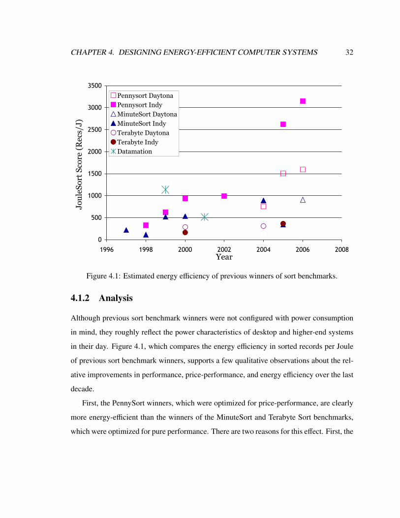
Figure 4.1: Estimated energy e!ciency of previous winners of sort benchmarks.
4.1.2 Analysis
Although previous sort benchmark winners were not configured with power consumption
in mind, they roughly reflect the power characteristics of desktop and higher-end systems
in their day. Figure 4.1, which compares the energy e!ciency in sorted records per Joule
of previous sort benchmark winners, supports a few qualitative observations about the rel-
ative improvements in performance, price-performance, and energy e!ciency over the last
decade.
First, the PennySort winners, which were optimized for price-performance, are clearly
more energy-e!cient than the winners of the MinuteSort and Terabyte Sort benchmarks,
which were optimized for pure performance. There are two reasons for this e"ect. First, the

CHAPTER 4. DESIGNING ENERGY-EFFICIENT COMPUTER SYSTEMS 33
price-performance metric provides an incentive for system designers to use fewer compo-
nents, and thus less power. Second, it rewards the use of cheaper commodity components,
which, for a given performance point, traditionally have used less energy than expensive,
high-performance components.
In addition to being more energy-e!cient than performance-optimized systems, cost-
conscious systems have also shown much more improvement in energy e!ciency over
time. This lack of energy-e!ciency improvement over time for cluster hardware was also
noted by Barroso in 2005 [4].
Much of the energy-e!ciency improvement among the PennySort winners is due to the
last two winners in the Indy category. The 2005 winner, Sheenk Sort [77], benefited from
algorithmic improvements and a minimal hardware configuration–but most importantly,
trends in CPU design had finally swung toward energy e!ciency. The processor used
in Sheenk Sort had six times the clock frequency of the processor used by the previous
PennySort winner, while only consuming twice the power. Overall, Sheenk Sort had triple
the performance of the previous winner, while consuming only twice the power.
The 2006 PennySort winner, GPUTeraSort [21], improved upon its predecessors’
energy e!ciency by introducing a new system component, the graphics processing unit
(GPU), and utilizing it very e"ectively. The chosen GPU, the NVidia 7800 GT, is inex-
pensive and comparable in estimated power consumption (57 W) to the system’s 3 GHz
Pentium IV CPU (80 W), but the GPU provides much better streaming memory bandwidth
than the CPU.
The success of GPUTeraSort shows the danger of relying on energy benchmarks that
focus only on specific hardware like CPU or disks, rather than end-to-end e!ciency. Such
specific benchmarks would only drive and track improvements of existing technologies and
may fail to anticipate the promise of potentially disruptive technologies.
Table 4.1 compares the growth rates of previous sort benchmark winners along three
dimensions: performance (sorted records per second), price-performance (sorted records

CHAPTER 4. DESIGNING ENERGY-EFFICIENT COMPUTER SYSTEMS 34
Benchmark SRecs/sec SRecs/$ SRecs/JPennySort 51%/yr. 58%/yr. 25%/yr.Performance sorts 38%/yr. n/a 13%/yr.
Table 4.1: Estimated yearly improvement in pure performance (SRecs/sec), price-performance (SRecs/$), and energy e!ciency (SRecs/J) of past Sort Benchmark winners.Performance sorts include MinuteSort, Terabyte Sort, and Datamation Sort.
per dollar), and energy e!ciency (estimated sorted records per Joule). The benchmarks are
divided into two categories according to the benchmark’s goal: price-performance and pure
performance. For each category, the yearly rate of improvement is calculated by choosing
the best system (according to the metric) in each year and fitting the result with an exponen-
tial. Table 4.1 shows that PennySort systems are improving almost at the pace of Moore’s
Law along the performance and price-performance dimensions. The pure performance sys-
tems, however, are improving much more slowly.
This analysis also shows much slower growth in estimated energy e!ciency than in
the other two metrics for both benchmark categories. Therefore, either energy e!ciency
is improving much more slowly than the other metrics, or the current benchmarks are not
capturing the most energy-e!cient systems. The 2006 PennySort winner sorts an estimated
3,200 records per Joule, but the 2007 JouleSort winner sorts 11,600 records per Joule (see
Section 4.3), rather than the 4,000 expected from extrapolating the yearly trends. This
result suggests that a benchmark focused on energy e!ciency is necessary to track trends
and to promote development of energy-e!cient systems and technologies, independent of
cost considerations.

CHAPTER 4. DESIGNING ENERGY-EFFICIENT COMPUTER SYSTEMS 35
Name DescriptionLaptop Core 2 Duo-based Compaq NC6400 laptopBlade Transmeta E!ceon-based HP low-power blade serverStd Server Xeon-based HP Proliant DL360 G3 standard 1U serverFileserver Xeon-based HP Proliant DL360 G5 + disk trays (see Section 4.2.2)
Table 4.2: Summary of commodity systems for which the JouleSort rating was experimen-tally measured.
4.2 Evaluation of Commodity Systems
This section describes the results of running the JouleSort benchmark on a variety of com-
modity systems, from laptops to servers. The “unbalanced” systems are presented to ex-
plore the system hardware space with respect to power consumption and energy e!ciency
during sort; they are “unbalanced” in the sense of not being tuned to exactly match CPU
sorting bandwidth with I/O bandwidth. In addition, a “balanced” fileserver, with a hard-
ware configuration tuned for the JouleSort benchmark, is presented as the default 2007 1
TB benchmark winner. Insights from these balanced and unbalanced commodity systems
are used to construct the 100 GB JouleSort winner, presented in Section 4.3.
4.2.1 Unbalanced Systems
Configurations
Tables 4.2 and 4.3 show the details of the unbalanced systems that were evaluated, com-
prising a variety of servers and personal computers. They include a standard server, an
older low-power blade, and a modern (circa 2006) laptop with its display turned o" for
these experiments. The blade was housed in an enclosure designed to hold 15 blades; nev-
ertheless, according to the benchmark rules, the wall power for the entire enclosure is used
to compute the benchmark score.

CHAPTER 4. DESIGNING ENERGY-EFFICIENT COMPUTER SYSTEMS 36
System CPU Memory Disk(s) OSLaptop Intel Core 2 Duo 3 GB 1!SATA, 60 GB, Win XP
T7200, 2 GHz DDR2 7200 rpmBlade Transmeta E!ceon 256 MB 1!IDE, 36 GB, Win 2K
TM8000, 1 GHz SDRAM 5400 rpmStd Server Intel Xeon, 2.8 GHz 2 GB 2!SCSI, 36 GB, Linux
DDR 15000 rpm (Fedora)
Table 4.3: Specifications of the unbalanced commodity systems listed in Table 4.2.
System Recs Power (W) Time (sec.) SRecs/J CPU util.
Laptop 50M 21.0 ± 1.0 727.5 ± 28 3270 ± 120 1%100M 21.7 ± 1.0 1323 ± 48 3479 ± 131 1%
Blade 50M 90.0 ± 1.0 1847 ± 52 300 ± 10 11%
Std server 50M 139.3 ± 0.1 299.4 ± 2.5 1206 ± 10 25%100M 138.5 ± 0.1 596.9 ± 0.6 1203 ± 1 26%
Table 4.4: JouleSort benchmark scores of unbalanced commodity systems.
The sort software used in all experiments was Ordinal Technology’s commercial Nsort
program [48], which was used in the winning entry of the 2006 Daytona Terabyte Sort
competition. Nsort uses asynchronous I/O to overlap reading, writing, and sorting oper-
ations as much as possible. It performs both one and two-pass sorts. For each platform,
Nsort’s parameters were tuned for maximum performance. Unless otherwise specified, all
experiments use radix sort for the in-memory sorting algorithm.
To measure the full-system AC power consumption, a digital power meter was inter-
posed between the system being tested and the wall outlet, and samples were taken once
per second. The meter used was the Brand Electronics Model 20-1850CI, which reports
true power with +/- 1.5% accuracy. All measured results show the average power and its
standard deviation over several trials.

CHAPTER 4. DESIGNING ENERGY-EFFICIENT COMPUTER SYSTEMS 37
Results
Table 4.4 shows the JouleSort benchmark scores for these unbalanced systems. Since disk
space on these systems was limited, the benchmark was run with data sets of 50 million
records (5 GB) and, when possible, 100 million records (10 GB). The power factors for
these systems were 1.0 for the server, 0.92 for the blade, and 0.55 for the laptop, reflecting
the fact that mobile devices are not typically designed with power factor correction.
The results show that the standard server is by far the fastest system, taking less time
to sort 100 million records than either the blade or the laptop takes to sort just 50 million
records. However, the laptop is clearly the most energy-e!cient machine: the server is 2.2
times as fast as the laptop but uses 6.6 times as much power. Although the standard server’s
disks should be able to provide substantially more sequential bandwidth than the other two
systems’ mobile disks, the server is limited by its SmartArray 5I I/O controller to just 33
MB/s in each pass.
The blade system’s showing is deceptively poor, because measuring the wall power
requires taking the full enclosure power into account. Since the enclosure is designed to
power up to 15 blades, it is both overprovisioned and ine!cient at the low load of a single
blade. If the power consumption is adjusted to reflect the blade itself plus a proportionate
share of the enclosure power, the JouleSort rating becomes 1121 ± 144 sorted records per
Joule, considerably higher than the result shown in Table 4.4.
The results also show that the CPUs in all three systems were severely underutilized.
In particular, the laptop attains an energy e!ciency similar to that of GPUTeraSort, even
though its cores are barely utilized. Since the CPU is usually the the most power-hungry
system component, and since CPUs are more energy-e!cient at high utilization, these
results suggest that the laptop’s energy e!ciency would dramatically increase if it had
enough I/O to complement the available processing capacity.

CHAPTER 4. DESIGNING ENERGY-EFFICIENT COMPUTER SYSTEMS 38
4.2.2 Balanced Server
This section presents a commodity fileserver in which the number of disks was adjusted to
match I/O bandwidth with CPU sorting bandwidth as closely as possible. Table 4.5 lists
the components of the server along with estimates of component power. The main system
is an HP Proliant DL360 G5 that includes a motherboard, a CPU and memory, a low-power
laptop disk, and a high-throughput SAS I/O controller. Additional storage is provided by
two disk trays, one of which holds the input and output files, and the other of which holds
the temporary data. Each tray can house up to 12 disks. The disk trays and the main system
all have dual power supplies but were powered with one each for these experiments. For
all of these experiments, the operating system was 64-bit Ubuntu Linux with the XFS file
system.
As Table 4.5 shows, the two populated disk trays consume roughly the same power as
the main system. When a tray is fully populated with 12 disks, its idle power is 145 W; with
six disks, the idle power is 101 W, showing potential energy ine!ciencies when the tray is
not fully populated. To estimate the power consumed by the memory, two 1 GB DIMMs
were installed in the system, and the system power was measured with and without the 2
GB DIMMs described in Table 4.5. These experiments showed that the 2 GB DIMMs use
7.5 W each, both during the sort and when idle.
Initial experiments to determine the optimum hardware configuration for this system
were conducted using a 10 GB data set. Even though underpopulating the disk trays seems
ine!cient, the best-performing 10 GB setup uses 12 disks split across the two trays. This
e"ect occurs because the system’s I/O controller o"ers better bandwidth when both of
its channels are used than when all 12 disks use a single channel. For a 10 GB sort, the
controller provides 313±1 MB/s of I/O bandwidth when the disks are split across both trays,
but only 212±1 MB/s when the disks are confined to a single tray. The average power of the
system is 406±1 W with two trays and 347±1 W with just one tray. As a result, the better

CHAPTER 4. DESIGNING ENERGY-EFFICIENT COMPUTER SYSTEMS 39
Component Model Idle Power Sort PowerCPU Intel Xeon 5130, 2 GHz 65 W (TDP)Memory 2!2GB PC2-5300 7.5 ± 0.5 W (each)OS disk 1!Fujitsu SATA, 5400rpm, 60GB n/aI/O Ctrl. LSI Logic SAS HBA 3801E n/aMotherboard HP Proliant DL360G5 n/aTotal of above 168±1 W 181±1 WDisk trays 2!HP MSA60, each with 101±1W 113±1 W
6!Seagate Barracuda ES, (each) (each)SATA, 7200rpm, 500GB
Table 4.5: Specifications of the balanced fileserver.
configuration is the two-tray setup, which sorts 3863±19 records per Joule. The one-tray
setup sorts only 3038±22 records per Joule.
The 2-tray, 12-disk setup is also the point where the I/O and CPU bandwidths match.
When the number of disks is reduced to 10, the performance and CPU utilization drop, and
the power saved by eliminating two disks is outweighed by the drop in performance. When
the number of disks is increased to 14, the sort is CPU-bound, and so the performance and
CPU utilization remain the same as with 12 disks. In this case, the increase in power from
the two additional disks does not provide any performance gain. The balanced 12-disk
configuration is thus the most energy-e!cient point.
Table 4.7 shows the performance and energy characteristics of this system for a 1 TB
sort. This system takes nearly three times as much power as the standard server, but it
provides over eight times the throughput. This system’s sorted records per Joule ratio is
higher than both the laptop’s score and the score estimated for GPUTeraSort, even though
it is using a much larger data set. With a 1 TB data set, the fileserver’s two cores are fully
utilized, and the I/O sorting bandwidth closely matches the CPU bandwidth. Experiments
similar to those conducted with the 10 GB data set show that this is also the optimal con-
figuration at the 1 TB scale. In both cases, the most energy-e!cient and best-performing

CHAPTER 4. DESIGNING ENERGY-EFFICIENT COMPUTER SYSTEMS 40
configuration occurs when the sort is CPU-bound and the I/O bandwidth closely matches
the CPU bandwidth.
4.2.3 Summary
These experiments with balanced and unbalanced systems show that the most energy-
e!cient server configuration occurs when the system is CPU-bound, and that a laptop
with an enormous mismatch between CPU and I/O sorting bandwidth is nearly as energy-
e!cient as a balanced server. These results suggest that a mobile processor backed with
adequate I/O bandwidth would be a highly energy-e!cient sorting system. To provide the
I/O bandwidth, laptop drives consume about five times less power than the file server’s
SATA drives while o"ering approximately half the bandwidth. Therefore, a promising ap-
proach to building the most energy-e!cient sorting system is to use mobile-class CPUs and
disks and connect them via a high-speed I/O interconnect.
4.3 Design of the JouleSort Winner
Using the lessons from running the JouleSort benchmark on commodity hardware, the next
goal was to create an energy-e!cient machine that convincingly overtook the other mea-
sured and estimated systems. For simplicity, the system was composed of commercially
available components, and Nsort was used as the software. The strategy for building this
machine was to create a balanced sorting system out of low-power components. The man-
ufacturer specifications of a variety of low-power x86 processors and mobile disks were
examined to estimate the sorting e!ciency of potential systems, resulting in the config-
uration shown in Table 4.6. This machine, nicknamed CoolSort, is over 3.5 times more
energy-e!cient than any of the systems described in the previous sections.

CHAPTER 4. DESIGNING ENERGY-EFFICIENT COMPUTER SYSTEMS 41
Component Model Price ($) Power (W)CPU Intel Core 2 Duo T7600 639.99 34 (TDP)Motherboard Asus N4L-VM DH 108.99Case/PSU APEVIA X-Navigator 94.99
ATXA9N-BK/5008-disk RAID card HighPoint Rocket RAID 2320 249.99 9.54-disk RAID card HighPoint Rocket RAID 2300 119.99 2.0Memory (2) Kingston 1GB DDR2 667 63.99 1.9W (spec)Disk (13) Hitachi TravelStar 5K160, 119.99 Active: 1.8
5400 rpm, 160 GB Idle: 0.85Adapters 130.25
Total 3032.05 Active: 100Idle: 59
Table 4.6: Components of the CoolSort machine and their retail prices at the time of pur-chase.
4.3.1 Details of Winning Configuration
This system uses a high-end mobile CPU with five frequency states and a TDP of 34W for
the highest frequency state. The choice of motherboard was somewhat constrained; few
boards support both a mobile CPU and enough I/O bandwidth to achieve a balanced sort.
The chosen motherboard, the Asus N4L-VM DH, has two SATA connectors on the moth-
erboard and two PCI-Express slots: one 1-channel and one 16-channel. To fill those slots,
CoolSort uses two RAID controllers, one of which holds four disk drives and one of which
holds eight. Connected to those controllers and to the motherboard are 13 low-power SATA
laptop disks. According to their manufacturer specifications, their average seek time is ap-
proximately 11 ms [29], and their sequential bandwidth through the XFS file system was
measured to be 45 MB/s in experiments with CoolSort. The manufacturer specifications
list an average power consumption of 1.8 W when reading and writing and 0.85 W in the
active idle state (idle but not sleeping) [29]. For memory, CoolSort uses two 1 GB DIMMs
that each consume 1.9 W of power, according to the manufacturer specifications [35].

CHAPTER 4. DESIGNING ENERGY-EFFICIENT COMPUTER SYSTEMS 42
System Recs SRecs/J Energy (kJ) Power (W) Time (sec)CoolSort 108 11628 ± 41 8.6 ± 0.03 99.3 ± 0.2 86.6 ± 0.4(Table 4.6) 109 11354 ± 29 88.1 ± 0.23 100.0 ± 0.1 880.8 ± 1.5Fileserver 1010 3425 ± 40 2920 ± 0.34 406 ± 1 7196 ± 67(Table 4.5)
Table 4.7: Power and performance of winning JouleSort systems.
System Recs Bandwidth (MB/s) CPU util. PFInput Output Total (200 max.)
CoolSort 108 248 ± 3 222 ± 1 115 ± 1 139 ± 1% 0.65109 238 ± 0.1 219 ± 0.4 114 ± 0.2 154 ± 0%Fileserver 1010 274 ± 0.4 282 ± 5 139 ± 1 179 ± 2% 0.96
Table 4.8: Detailed utilization information for winning JouleSort systems, including thenumber of sorted records, the sorting bandwidths and CPU utilization, and the power factor(PF).
The optimal configuration uses 13 disks because the PCI-e RAID cards hold a maxi-
mum total of 12 disks, and the I/O performance of the motherboard controller with more
than one disk is poor. The input and output files are striped across a 6-disk array configured
via LVM2, and the remaining 7 disks are independent for the temporary data. All experi-
ments use Linux kernel 2.6.18 and the XFS file system unless otherwise stated. In the idle
state at the lowest CPU frequency, this system consumes 59.0 ± 1.3 W of power.
Tables 4.7 and 4.8 show the performance of the system, which attains 11,628 sorted
records per Joule when averaged over three consecutive runs. The pure-performance statis-
tics are reported by Nsort. Nsort was configured to use radix sort as its in-memory sort
algorithm and to use transfer sizes of 4 MB for the input-output array and 2 MB for the
temporary data. This system sorts 24% faster than GPUTeraSort and consumes an esti-
mated one-third of the power. The power use during sort is 69% more than when idle.
During the output pass, the CPU is underutilized (see Table 4.8; note that the maximum
utilization for 2 cores is 200%), and the sorting bandwidth is lower than in the input pass

CHAPTER 4. DESIGNING ENERGY-EFFICIENT COMPUTER SYSTEMS 43
because the output pass requires more random I/O. The CPU frequency state is pinned to
1660 MHz, which Section 4.3.3 shows is the most energy-e!cient frequency for the sort.
4.3.2 Varying Hardware Configuration
This section examines the performance, cost e!ciency, and energy e!ciency of varying
the disk configuration, amount of memory, and power supply of the CoolSort system.
Disks and RAID Controllers
This section examines the relationship between the number of disks and controllers and
the system’s performance, cost e!ciency, and energy e!ciency. These experiments were
performed using a 5 GB data set for speed; the results should qualitatively hold for larger
data sets, since this data set is considerably larger than the available memory. The CPU
was set to its highest frequency for the experiments involving performance and cost ef-
ficiency in order to maximize these metrics, since both metrics reward performance and
do not consider power consumption. All experiments began with 2 disks attached to the
cheaper 4-disk controller, and at each step, an additional disk was added to maximize cost
e"ectiveness. Therefore, the 8-disk controller alone is used for configurations with 5–8
disks, and both controllers are combined for 9–12 disks. Finally, a disk is added directly
to the motherboard for the 13-disk configuration. The reason that the motherboard disk is
not used earlier is that the motherboard’s interface is slower than the controller interfaces,
creating a performance bottleneck for smaller configurations. Table 4.9 summarizes these
di"erent hardware configurations and their prices.
Figure 4.2 shows the performance (sorted records per second) and cost e!ciency
(sorted records per dollar) with increasing system size. The 13-disk configuration is
both the best-performing and most cost-e!cient point. On average, each additional disk
increases system cost by about 7% and improves performance by 14%. These marginal

CHAPTER 4. DESIGNING ENERGY-EFFICIENT COMPUTER SYSTEMS 44
# Disks 4-disk 8-disk Mother- Price ($)card card board2 2 1341.823 3 1471.754 4 1596.695 5 1856.626 6 1981.567 7 2111.498 8 2236.439 1 8 2486.35
10 2 8 2620.2811 3 8 2759.2012 4 8 2893.1313 4 8 1 3032.05
Table 4.9: CoolSort configurations with varying numbers of disks. For each number ofdisks shown in the left-hand column, the next three columns show the number of disksattached to the 4-disk controller, the 8-disk controller, and the motherboard, respectively.A controller is removed from the system if no disks are attached to it.
changes vary; they are larger for small system sizes and smaller for large system sizes. The
5-disk point drops in cost e!ciency because it requires moving from the 4-disk controller
to the more expensive 8-disk controller without a commensurate performance increase.
Although the motherboard and controllers limit the system to 13 disks, additional disks
would probably not help since the first pass of the sort is CPU-bound.
The next set of experiments determines how energy e!ciency varies with with system
size. The results reflect the minimum-energy hardware configuration to support each ad-
ditional disk. The CPU frequency is pinned to 1660 MHz in these experiments to get the
best energy e!ciency (see Section 4.3.3). For convenience, an extra disk was kept on the
motherboard to run the OS, but it was unused in the sort except for the 13-disk configura-
tion. The power measurements include this disk, but its power consumption is negligible at
idle (less than 1 W).

CHAPTER 4. DESIGNING ENERGY-EFFICIENT COMPUTER SYSTEMS 45
0
5
10
15
20
25
30
35
40
0 2 4 6 8 10 12 14
Disks Used
Rec
ord
s S
ort
ed p
er $
(x
1E9
)
0
20
40
60
80
100
120
140
Rec
ord
s S
ort
ed p
er S
ec.
(x1E
4)
Price-Perf.Performance
Figure 4.2: Variation of performance and price-performance with the number of disks inthe CoolSort system.

CHAPTER 4. DESIGNING ENERGY-EFFICIENT COMPUTER SYSTEMS 46
0
20
40
60
80
100
1 2 3 4 5 6 7 8 9 10 11 12 13
Disks Used
Av
g.
Po
wer
(W
)
Sorting Power
Idle Power
Figure 4.3: Variation of power consumption with the number of disks in the CoolSortsystem.

CHAPTER 4. DESIGNING ENERGY-EFFICIENT COMPUTER SYSTEMS 47
Figure 4.3 shows idle power at the lowest frequency state versus average power during
sort at 1660 MHz for the system configurations shown in Table 4.9. With the system
idle and only the motherboard disk installed, the 8-disk controller uses 9.5 W and the 4-
disk controller uses 2.0 W. Thus, system sizes between 2 and 4 disks use only the 4-disk
controller, sizes between 5 and 8 disks use only the 8-disk controller, and both controllers
are used for 9 or more disks. Figure 4.3 shows jumps in power consumption at these
transitions. The idle line illustrates that the marginal power consumption of an idle disk is
0.95 ± 0.1 W. The marginal power of an actively sorting disk, on the other hand, averages
4.3±1.0 W at sizes smaller than 8 disks and 3.4±1.0 W for sizes of 9 or more disks. These
increases reflect not only the disk’s power consumption, but also the end-to-end dynamic
utilization of the CPU, disk controllers, and other components.
Figure 4.4 shows the energy e!ciency as the number of disks used in the sort is varied.
The curve is similar to the price-performance curve in Figure 4.2. The average increase in
energy at each step is 6%, while the average increase in performance is about 14%. The 5-
disk point is again a local minimum, because it incurs the power consumption of the larger
8-disk controller without enough disks to realize its potential performance benefits. The
sort fully utilizes the CPU in the most energy-e!cient configuration.
These experiments support two main observations. First, the similar shapes of the cost-
and energy-e!ciency curves reflect that the base dollar and energy costs of the system are
high compared to the marginal dollar and energy costs of disks. If the system had used
server-class disks, which are similar in cost to mobile disks but consume five times the
power, the shapes of the cost- and energy-e!ciency curves would di"er from each other.
Second, for the components chosen, the best-performing, most cost-e!cient, and most
energy-e!cient configurations are identical, except for the CPU frequency. This is the
point where the I/O bandwidth balances the CPU bandwidth, and the sort is CPU-bound in
the input pass.

CHAPTER 4. DESIGNING ENERGY-EFFICIENT COMPUTER SYSTEMS 48
0
2000
4000
6000
8000
10000
12000
1 2 3 4 5 6 7 8 9 10 11 12 13
Disks Used
Rec
ord
s S
ort
ed p
er J
ou
le
0
20
40
60
80
100
120
140
Rec
ord
s S
ort
ed P
er S
ec.
(x1E
4)
Recs/J
Performance
Figure 4.4: Variation of energy e!ciency with the number of disks in the CoolSort system.

CHAPTER 4. DESIGNING ENERGY-EFFICIENT COMPUTER SYSTEMS 49
Memory and Power Supply
For two-pass sorts, which do not fit in memory and thus require temporary writes to disk,
adding memory to the system does not necessarily improve performance. For most of the
experiments described in this chapter, the Nsort software elected to use only a fraction of
the available memory. Experimenting with only one 1 GB DIMM in the system resulted
in power use and execution time that were statistically indistinguishable from the 2-DIMM
configuration outlined in Section 4.3.1. The power consumption di"erence for the idle state
also fell within measurement error.
The configuration described in Section 4.3.1 used a 500 W power supply that came
with the system’s case. Since many power supplies are ine!cient at low loads, and since
CoolSort’s 100 W is far below the power supply’s rated load, experiments replacing the
500 W power supply with a 145 W power supply were conducted. However, the power
consumption both while sorting and while idle increased by 2 W over the original 500 W
power supply. This results suggests that at 68% load or less, e!ciencies of the two power
supplies are similar. It also suggests that power supply e!ciency varies on a case-by-
case basis; since the goal of this work was not to exhaustively compare individual power
supplies, the 500 W power supply was chosen and no further experiments were conducted.
The power factors for the laptop- and desktop-based systems described in this chapter,
including CoolSort, are far below 1.0. Low power factors are problematic in data cen-
ters, because they require power delivery mechanisms to be overprovisioned to carry addi-
tional current. Utility companies often charge for this extra provisioning. For systems like
CoolSort to be adopted in data centers, they will need to use power supplies that provide
power-factor correction, as server power supplies do.

CHAPTER 4. DESIGNING ENERGY-EFFICIENT COMPUTER SYSTEMS 50
0
50
100
150
200
996 1328 1660 1992 2324 On
DemandCPU Freq. (MHz)
Av
g.
Po
wer
(W
)
0
2000
4000
6000
8000
10000
12000
Rec
ord
s S
ort
ed p
er J
ou
le
XFS, radix (W) Reiser, radix (W) XFS, merge (W)
XFS, radix (SRecs/J) Reiser, radix (SRecs/J) XFS, merge (SRecs/J)
Figure 4.5: Variation of average power and energy e!ciency with CPU frequency andfilesystem for a 10 GB sort on CoolSort.

CHAPTER 4. DESIGNING ENERGY-EFFICIENT COMPUTER SYSTEMS 51
4.3.3 Varying Software Configuration
The next experiments vary the file system and in-memory sorting algorithm to see how they
a"ect energy e!ciency. The winning 10 GB configuration uses the XFS file system and a
radix sort. Figure 4.5 examines the e"ect of changing the file system to ReiserFS and the
sort algorithm to merge sort at di"erent CPU frequencies.
As expected, power consumption steadily increases with frequency in all cases. The
power consumptions of XFS with radix sort and merge sort are similar at all frequencies.
ReiserFS, however, consumes less power and also is less energy-e!cient. All three config-
urations show improved energy e!ciency from 996 MHz to 1660 MHz, and then level o"
or decrease. This result indicates that the sorts are CPU-bound, and thus benefit from in-
creased CPU performance, at the lower frequencies. ReiserFS shows a 26% improvement
in performance between the lowest and highest frequencies, while XFS radix improves
only 16% and XFS merge improves only by 20%.
ReiserFS has lower energy e!ciency mainly because it provides less sequential band-
width, and thus lower performance, than XFS. Although each configuration was tuned, this
result may be an artifact of this particular system and not an inherent flaw of ReiserFS.
Similarly, the merge sort has lower energy e!ciency than radix sort entirely because its
performance is worse.
The rightmost part of the graph shows the power and energy e!ciency of the Linux on-
demand CPU frequency scaling policy, which is within 10% of the fastest execution time
and 15% of the lowest power for all three configurations. For ReiserFS, the on-demand
policy o"ers the same energy e!ciency as the best configuration. In summary, these ex-
periments show that the algorithms and underlying software used for sort a"ect energy
e!ciency mainly through performance, and that the question of which sorting algorithm is
most energy-e!cient is still open.

CHAPTER 4. DESIGNING ENERGY-EFFICIENT COMPUTER SYSTEMS 52
4.3.4 CPU and I/O Dynamic Power Variation
To determine the individual contributions of the I/O subsystem (disks plus controllers)
and the CPU subsystem (CPU plus memory) to the dynamic power variation during sort,
several microbenchmarks were run. In the 12-disk configuration, the system consumes 33.5
W more power during sort than when the system is idle with the same CPU frequency. This
dynamic variation accounts for nearly 35% of the total power during sort. The experiments
described below suggest that the I/O subsystem consumes a greater fraction of this dynamic
power increase than the CPU subsystem.
The first experiment was a disk-intensive microbenchmark intended to determine the
contribution of the I/O subsystem. This experiment copied data from a 6-disk array to
another 6-disk array, using the same average disk bandwidth as the 12-disk sort. During
this experiment, the system power increased by 30.5 W over the idle power. The CPU
utilization was 66% out of a possible 200% for 2 cores. The next experiment was designed
to approximate the contribution of the CPU subsystem, and consisted of repeatedly sorting
a small input file mounted on a RAM disk. This test pegged the CPU at 200% utilization,
and the power increase was 15.7 W over the idle power.
Using the above results and assuming that CPU subsystem power increases linearly
with CPU utilization, its contribution to the total power increase during the 12-disk sort
can be estimated as follows. During the sort, CPU utilization averaged 118% (59% per
core). Scaling the power increase of 15.7 W at 200% utilization down by 0.59 yields a
9.2 W contribution from the CPU subsystem during sort. Now the contribution of the I/O
subsystem can be estimated by subtracting the estimated CPU power from the total power
increase during the copying experiment. This estimate of 30.5 W#0.33!15.7 W = 25.3 W.
Combining these estimates yields a total dynamic power increase of 34.5 W, which comes
within 3% of the 33.5 W measured increase during the 12-disk sort. These tests thus imply

CHAPTER 4. DESIGNING ENERGY-EFFICIENT COMPUTER SYSTEMS 53
that about 75% of the power increase during sort is from the I/O subsystem and 25% from
the CPU subsystem. Experiments done at smaller system sizes found similar proportions.
4.3.5 Summary
This section described the winning Daytona 100 GB JouleSort system, which is over 3.5
times as energy e!cient as last year’s PennySort winner, GPUTeraSort. For this system,
the most energy-e!cient configuration is also the best-performing and most cost-e!cient,
a relationship that may be the result of using mobile disks rather than server disks. Experi-
ments showed that the choice of filesystem and in-memory sort algorithm mainly a"ected
energy e!ciency through performance rather than through power consumption for this sys-
tem.
The goal of this work was to build a balanced system with low-power o"-the-shelf
components targeted for the 100 GB scale. Unfortunately, because of the available sizes
of mobile disks, the CoolSort machine could not easily be scaled to the 1 TB category.
Other types of systems may be more e!cient in the 10 GB and 1 TB categories, but for
completeness, Tables 4.7 and 4.8 show the best configurations for those categories that
were encountered in these experiments.
4.4 Other Energy-E!ciency Metrics
Although JouleSort addresses a computer system’s energy e!ciency, energy is just one
piece of the system’s total cost of ownership (TCO). From a system purchaser’s perspective,
a TCO-Sort would be the most desirable sort benchmark; however, the components of
TCO vary widely from user to user. Combining JouleSort and PennySort to benchmark
the costs of purchasing and powering a system is a possible first step, although the current
sort benchmark metrics omit reliability, manageability, and security issues. This section
examines alternative possible metrics for an energy-aware sort benchmark using various

CHAPTER 4. DESIGNING ENERGY-EFFICIENT COMPUTER SYSTEMS 54
Name Description Price ($) Avg Pwr (W)Gumstix Used in embedded devices 376.50 2Soekris Used for networking apps 477.50 6VIA Multimedia machine with flash drives 1156.60 15
Table 4.10: Low-power machines benchmarked by Meza et al. [45].
weighings of price, performance, and power, and compares the types of systems that each
favors. All of these comparisons are subject to the caveats described in Sections 4.1.1
and 3.2.2: that is, they illuminate broad trends, but they are not precise measurements.
The machines compared in this section are the historical PennySort, Terabyte Sort, and
MinuteSort benchmark winners discussed in Section 4.1, the balanced fileserver described
in Section 4.2.2, the CoolSort machine discussed in Section 4.3.1, and three additional
ultra-low-power sorting systems designed by Justin Meza et al [45]. Table 4.10 summa-
rizes these systems and their JouleSort results. The first is an ARM-based Gumstix device,
typically used in embedded devices. The second is an AMD Geode-based Soekris board,
designed for routers and networking equipment. The final machine is a VIA picoITX em-
bedded multimedia machine with flash hard drives.
Figures 4.6 and 4.7 show the PennySort and JouleSort scores, respectively, of all of
these systems. Note that the ultra-low-power machines were only able to sort very small
data sets (less than 10 GB) with the amount of storage they had; for purposes of compar-
ison, CoolSort’s performance on a similarly sized data set (CoolSort-1 pass) is included.
All of these scores are normalized to the lowest-performing system in order to facilitate
comparisons among the di"erent metrics in addition to the di"erent machines. Note that
the balanced fileserver and the winners of the purely performance-based sort benchmarks
are not included in the comparisons of metrics involving cost, such as PennySort.
The PennySort results are dominated by GPUTeraSort, followed by two recent Pen-
nySort winners (BSIS [30] and Sheenk Sort) and CoolSort. Since mobile components,

CHAPTER 4. DESIGNING ENERGY-EFFICIENT COMPUTER SYSTEMS 55
0
5
10
15
20
25
30
35
40
CoolS
ort
1-
pass
CoolS
ort
2-
pass
Gum
stix
Soekri
s
VIA
BSIS
(2006)
GPU
Tera
Sort
(2006)
Post
man
Sort
(2005)
SheenkSort
(2005)
TH
Sort
(2004)
DM
Sort
(2002)
HM
Sort
(2000)
NTSort
(1998)
Energy-aware systems PennySort winners
No
rma
lize
d P
enn
yS
ort
Sco
re
Figure 4.6: PennySort scores of energy-aware systems and previous PennySort benchmarkwinners, normalized to the lowest-scoring system.
such as those used in CoolSort, usually cost a premium compared to their desktop equiv-
alents, this result is somewhat surprising. This cost premium also penalizes the ultra-low-
power components used in the other energy-aware systems, resulting in their low rankings
according to this metric.
The JouleSort results in Figure 4.7 show that all of the energy-aware machines out-
perform all of the historical PennySort winners, although the Gumstix, the fileserver, and
GPUTeraSort are roughly equivalent. Among the ultra-low-power machines, the VIA in
particular comes close to the energy e!ciency of CoolSort’s two-pass sorts. This result
illustrates the energy-e!ciency potential of ultra-low-power, flash-based systems.
Figures 4.8 and 4.9 combine performance, price, and power in two di"erent ways.
Figure 4.8 evaluates systems based on their JouleSort rating per dollar (records per Joule per

CHAPTER 4. DESIGNING ENERGY-EFFICIENT COMPUTER SYSTEMS 56
0
10
20
30
40
50
60
70
80
90
100
CoolS
ort
1-
pass
CoolS
ort
2-
pass
Gum
stix
Soekri
s
VIA
Filese
rver
BSIS
(2006)
GPU
Tera
Sort
(2006)
Post
man
Sort
(2005)
SheenkSort
(2005)
TH
Sort
(2004)
DM
Sort
(2002)
HM
Sort
(2000)
NTSort
(1998)
NeoSort
(2006)
SCS (
2005)
Nso
rt (
2004)
SPSort
(2000)
HPVM
Sort
(1999-2
000)
Now
Sort
(1997-1
998)
Energy-aware systems PennySort winners MinuteSort and TerabyteSort
winners
No
rm
ali
ze
d J
ou
leS
ort
Sco
re
Figure 4.7: JouleSort scores of energy-aware systems and previous PennySort, MinuteSort,and Terabyte Sort benchmark winners, normalized to the lowest-scoring system.

CHAPTER 4. DESIGNING ENERGY-EFFICIENT COMPUTER SYSTEMS 57
0
5
10
15
20
25
30
35
40
45
CoolS
ort
1-
pass
CoolS
ort
2-
pass
Gum
stix
Soekri
s
VIA
BSIS
(2006)
GPU
Tera
Sort
(2006)
Post
man
Sort
(2005)
SheenkSort
(2005)
TH
Sort
(2004)
DM
Sort
(2002)
HM
Sort
(2000)
NTSort
(1998)
Energy-aware systems PennySort winners
No
rma
lize
d (
Re
cord
s /
J /
$)
Figure 4.8: Records sorted per Joule per dollar of purchase price of energy-aware systemsand previous PennySort winners, normalized to the lowest-scoring system.
dollar), using the list price of the system. Compared to the JouleSort and PennySort metrics,
this metric gives extra weight to resource constraints: the PennySort and JouleSort metrics
can be abstracted as performance divided by a resource constraint (price or power), while
this metric is equivalent to performance divided by the product of two resource constraints.
Since price and power consumption somewhat correlate, as explained in Section 4.1.2,
this metric should favor smaller systems with lower power and lower price. Indeed, this
metric is where the ultra-low-power systems shine, far outstripping the historical PennySort
winners and the other energy-e!cient systems. CoolSort and the minimally configured
Sheenk Sort come in a distant fourth and fifth. In a situation where resource constraints are
the primary concern, these ultra-low-power machines are the best choice.

CHAPTER 4. DESIGNING ENERGY-EFFICIENT COMPUTER SYSTEMS 58
1
10
100
1000
10000
CoolS
ort
1-
pass
CoolS
ort
2-
pass
Gum
stix
Soekri
s
VIA
BSIS
(2006)
GPU
Tera
Sort
(2006)
Post
man
Sort
(2005)
SheenkSort
(2005)
TH
Sort
(2004)
DM
Sort
(2002)
HM
Sort
(2000)
NTSort
(1998)
Energy-aware systems PennySort winners
No
rma
lize
d J
ou
leS
ort
-Pen
ny
So
rt P
rod
uct
Figure 4.9: Product of JouleSort and PennySort scores of energy-aware systems and previ-ous PennySort winners, on a logarithmic scale, normalized to the lowest-scoring system.

CHAPTER 4. DESIGNING ENERGY-EFFICIENT COMPUTER SYSTEMS 59
Figure 4.9, on the other hand, keeps PennySort and JouleSort’s one-to-one balance
between performance and resource constraints by multiplying the PennySort and JouleSort
ratings to get a combination metric in Records2/(Joule ! sec), which is normalized to the
lowest-scoring system in the figure. Because of the great disparities in this rating among the
systems compared, Figure 4.9 uses a logarithmic scale. According to this metric, CoolSort
gives the best balance of performance and price/power, followed distantly by the VIA, the
Soekris, and the recent PennySort winners. This combined metric shows that the additional
cost of high-performance, low-power components does not prohibit them from being good
choices when price is taken into consideration.
Figure 4.10 does not consider price, but instead provides a di"erent weighing of perfor-
mance and power than the JouleSort metric. Rather than weighing performance and power
equally, it uses the energy-delay product, which privileges performance. The metric used is
(Records/Joule) ! (Records/sec.); because the machines being compared sorted varying
numbers of records, execution time must be normalized to the workload size to provide
a fairer comparison. Note that this metric is the inverse of the energy-delay product, so
higher scores are better. Again, because of the great disparities in this metric among the
di"erent systems, Figure 4.10 uses a logarithmic scale.
Because of the additional weight given to performance, the MinuteSort and Terabyte
Sort winners fare much better with this metric than with the original JouleSort metric, as
does the balanced fileserver. In general, this metric clearly favors larger systems than the
JouleSort metric. However, CoolSort remains the highest-ranked system according to this
metric, and the ultra-low-power VIA is surprisingly competitive at this metric that should
be biased against it.
Finally, Figure 4.11 attempts to synthesize a TCO estimate and compare the systems
based on their sorting performance per dollar of TCO. The performance metric used is the
number of records sorted per unit time. The metric used to approximate TCO is the initial
cost of the hardware plus an estimate of the energy cost of running the sort for three years
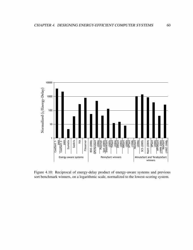
CHAPTER 4. DESIGNING ENERGY-EFFICIENT COMPUTER SYSTEMS 60
1
10
100
1000
10000
CoolS
ort
1-
pass
CoolS
ort
2-
pass
Gum
stix
Soekri
s
VIA
Filese
rver
BSIS
(2006)
GPU
Tera
Sort
(2006)
Post
man
Sort
(2005)
SheenkSort
(2005)
TH
Sort
(2004)
DM
Sort
(2002)
HM
Sort
(2000)
NTSort
(1998)
NeoSort
(2006)
SCS (
2005)
Nso
rt (
2004)
SPSort
(2000)
HPVM
Sort
(1999-2
000)
Now
Sort
(1997-1
998)
Energy-aware systems PennySort winners MinuteSort and TerabyteSort
winners
No
rma
lize
d (
1/E
ner
gy
-Del
ay
)
Figure 4.10: Reciprocal of energy-delay product of energy-aware systems and previoussort benchmark winners, on a logarithmic scale, normalized to the lowest-scoring system.

CHAPTER 4. DESIGNING ENERGY-EFFICIENT COMPUTER SYSTEMS 61
0
4
8
12
16
20
24
28
32
CoolS
ort
1-
pass
CoolS
ort
2-
pass
Gum
stix
Soekri
s
VIA
BSIS
(2006)
GPU
Tera
Sort
(2006)
Post
man
Sort
(2005)
SheenkSort
(2005)
TH
Sort
(2004)
DM
Sort
(2002)
HM
Sort
(2000)
NTSort
(1998)
Energy-aware systems PennySort winners
No
rma
lize
d P
erf
orm
an
ce/T
CO
$
Figure 4.11: Performance-TCO ratio for energy-aware systems, normalized to the lowest-scoring system.

CHAPTER 4. DESIGNING ENERGY-EFFICIENT COMPUTER SYSTEMS 62
at a cost of $100 per megawatt-hour [52]. The TCO estimates in the graph are computed
according to Equation 4.1. This equation does not include cooling or burdened costs.
TCO ($) = Price + AvgPwr (W) ! 24 hrday
! 365 daysyr
! 3 yr ! $100MWhr
! MW1E6 W
= Price + 2.628 ! AvgPwr (4.1)
Over three years, the TCO is thus the initial cost of hardware plus 2.6 times the average
power in Watts. For all of the machines in Figure 4.11, the initial purchase price is a larger
factor in this TCO metric than the estimated cost of energy; the initial cost is particularly
dominant for the energy-aware machines and the early PennySort winners. Using this
TCO-aware metric, GPUTeraSort fares best among the two-pass sorting configurations,
followed by CoolSort and Sheenk Sort. The overall graph is similar to the PennySort graph
(Figure 4.6), with slightly lower disparities between the best- and worst-scoring systems.
If cooling costs are factored in, the contribution of power consumption to the TCO rises,
and the graph begins to look more like the JouleSort graph (Figure 4.7). CoolSort passes
GPUTeraSort as the highest scorer when cooling costs reach 0.8 W per Watt of power
consumed by the computing equipment; in data centers, the cost of cooling is 0.5 to 1 W
for each Watt of compute power [50].
Comparing these alternative metrics leads to several conclusions. First, low-power
components are excellent choices for energy e!ciency even when cost is taken into ac-
count. Second, although di"erent weighings of performance and power privilege di"erent
system classes, the CoolSort mobile fileserver and the VIA multimedia machine are fairly
insensitive to changes in these weighings, remaining at or near the top tier of systems for
all of these metrics. These results indicate that systems with high JouleSort benchmark
scores do not become impractical when cost or performance concerns are emphasized.

CHAPTER 4. DESIGNING ENERGY-EFFICIENT COMPUTER SYSTEMS 63
4.5 Conclusions
This chapter compared the JouleSort scores of a variety of systems, including the esti-
mated scores of previous sort benchmark winners and the measured scores of o"-the-shelf
and specially designed machines. It also presented CoolSort, the machine which achieves
the highest known JouleSort score, with over 3.5 times the energy e!ciency of previous
sort benchmark winners. CoolSort is a fileserver built from a mobile processor and 13 lap-
top disks connected through server-class I/O interfaces, an unusual design that highlights
the potential of low-power mobile components in the data center. While CoolSort was op-
timized specifically for the JouleSort benchmark, this type of design has the potential to
be broadly useful. Finally, this chapter examined alternative benchmark metrics weighing
di"erent combinations of price, performance, and power. Di"erent combinations of these
metrics privilege di"erent types of systems, but CoolSort and two ultra-low-power sorting
systems scored well across several di"erent metrics.
These benchmark results show that JouleSort continues the Sort Benchmark’s tradi-
tion of identifying promising new technologies. CoolSort’s benchmark scores illustrate
that a server composed of mobile-class components is highly energy-e!cient, without
being prohibitively costly or low-performance. The VIA system’s success demonstrates
the potential of ultra-low-power processors and flash storage for energy-e!cient execution
of data-intensive applications. Finally, GPUTeraSort’s success among the historical sort
benchmark winners shows that the high performance of GPUs comes at a relatively small
energy cost, although this observation may not continue to hold as GPUs grow ever more
power-hungry.
JouleSort does not address all possible energy-e!ciency concerns. It targets data-
intensive applications running at peak energy e!ciency, which is equivalent to peak
utilization for today’s technologies. This design choice di"ers from the full-system
SPECpower ssj benchmark, which is CPU-intensive and compares the average energy

CHAPTER 4. DESIGNING ENERGY-EFFICIENT COMPUTER SYSTEMS 64
e!ciency across the utilization spectrum. As a single-system benchmark, JouleSort also
omits some metrics of importance in the data center. It does not account for losses in
power delivery at either the data center or the rack level, nor does it account for the
building cooling used to maintain the ambient temperature around the system. However,
the JouleSort benchmark is relevant to an important class of systems and has already led to
innovations and insights in energy-e!cient system design.

Chapter 5
Power Modeling Background
65

CHAPTER 5. POWER MODELING BACKGROUND 66
Accurate models of power consumption are crucial components of many schemes to
improve the energy e!ciency of computing equipment. In the initial design of components
and systems, power models are necessary because it is not feasible to build physical systems
to assess every design choice’s e"ect on power consumption. In the day-to-day operation
of computer systems, users and data center operators need to know how their usage patterns
a"ect a machine’s power consumption in order to maximize energy e!ciency, whether in a
single system or over an ensemble of systems. The next three chapters of this thesis address
power models appropriate for the real-time power management needs of the latter groups.
This chapter enumerates the desirable properties of this sort of power model and assesses
the suitability of previously proposed models based on these properties. Chapters 6 and 7
propose and evaluate a specific method for generating a family of high-level, real-time
power models. They show that this method creates models that are not only accurate, but
also general and portable to a broad range of systems.
5.1 Power Modeling Goals
An ideal power modeling framework suitable for use in real-time scheduling decisions
would meet several design criteria, which this section describes. Physical power measure-
ments alone cannot meet these criteria, since they cannot predict future power consump-
tion, nor do they provide a link between resource usage and power consumption, which is
necessary for energy-e!ciency optimizations.
Full-system: The models should relate usage information to the power of the entire
system rather than an individual component.
Accurate: The model must be su!ciently accurate to enable energy-e!ciency opti-
mizations. In this work, we define accuracy as less than 10% error in the average case,
although higher accuracies are certainly better and may be necessary for some optimiza-
tions.

CHAPTER 5. POWER MODELING BACKGROUND 67
Fast: The model must generate predictions su!ciently quickly to be useful in real-time
optimizations; this work assumes that one prediction per second is su!ciently fast.
Generic and Portable: The modeling framework should apply to as many systems as
possible. It should work for di"erent classes of systems (mobile, desktop, and enterprise);
di"erent processor families and di"erent memory technologies; di"erent power footprints
and dynamic ranges; and di"erent balances of components, rather than assuming that any
particular component will dominate the system. It should be easy to generate models for
a new system, and doing so should require neither exhaustive tuning nor extensive design
space exploration.
Inexpensive: Generating and using the model should not require expensive equipment.
Non-intrusive and low-overhead: Collecting the model inputs should not require in-
trusive adjustments to the hardware of the system, nor should it have significant software
overhead.
Simple: The model should be as simple as possible, both in terms of the number of in-
puts and the complexity of the model, while still providing su!ciently accurate predictions
to enable energy-saving optimizations.
5.2 Power Modeling Approaches
This section examines three approaches to power modeling: simulation-based detailed
models, detailed analytical models, and high-level black-box models. It discusses previ-
ous work using each approach and explains that work’s advantages and disadvantages with
respect to the goals outlined in Section 5.1. This thesis does not discuss thermal modeling,
although thermal models similar to some of the power models described in this chapter have
been developed at both the processor [61] and full-system [26] levels. Deploying thermal
models requires sensor infrastructure that power modeling does not, since the current am-
bient temperature is a major factor in temperature prediction. Furthermore, thermal models

CHAPTER 5. POWER MODELING BACKGROUND 68
tend to be more complicated than power models, since power is an instantaneous quantity
and temperature is a"ected by temperatures nearby in both time and space. Therefore, this
discussion is restricted to power models.
5.2.1 Simulation-based Power Models
One approach to power modeling is to integrate it into software that simulates the execu-
tion of programs on a particular system or component. This approach is typically used
by system designers who have already written performance simulators of their prospective
systems and wish to understand their power consumption characteristics as well. These
models range in detail and accuracy from fine-grained models with detailed circuit knowl-
edge to models that use a combination of architectural information and circuit parameters.
They can be highly accurate and do not require the use of expensive equipment, but they
typically fail to meet the rest of the goals for real-time models described in Section 5.1.
First, they are almost always component-specific rather than full-system models, since
it is di!cult to obtain such detailed knowledge of the many components in a computer.
They also tend to be slow, since making power predictions requires fully simulating the
component or system. They are neither generic nor portable, relying on the specific imple-
mentation details of a particular component and requiring specialized knowledge even to
be ported to components in the same family. They are not necessarily low-overhead, rely-
ing on knowledge of the specific instructions being executed on a machine. Finally, they
are not simple: they require a great deal of information about the system architecture and
state, and require simulation in order to relate that information to the power consumption.
Despite these models’ shortcomings for real-time use, however, their high accuracy makes
them worth examining both as possible upper bounds on accuracy and for their insights
about component or system behavior.

CHAPTER 5. POWER MODELING BACKGROUND 69
One of the first processor power models to use architectural information rather than
detailed circuit knowledge was Wattch, proposed by Brooks et al. in 2000 [8]. Wattch
integrates into the widely used SimpleScalar performance simulator [9], adding power pre-
dictions to that simulator’s performance information. Wattch abstracts the structures on
a processor into four main categories: array structures such as caches and register files;
fully-associative content-addressable memories such as TLBs; combinational logic such as
functional units; and clock-related circuitry. It leverages the CACTI cache models [76] to
estimate the power usage of each structure based on that structure’s size and number of
ports, the process technology, the amount of switching activity, the supply voltage, and the
clock frequency; this approach yields processor power estimates with an average error of
less than 15% (30% at the high end of the power range). Since it is processor-specific and
based on detailed knowledge of individual processor structures, the Wattch approach is too
low-level for a portable real-time full-system power modeling framework.
A higher-level approach was used in the Tempo simulator by Shafi et al. to simulate
the power consumption of the PowerPC 405GP embedded system-on-a-chip [60]. The
model associates energy consumption with individual architectural events, such as data
cache misses or TLB reads, and then predicts the energy consumption by counting these
events: that is, Epred = Eidle+#(ei!ni), where each i is an architectural event whose energy
ei is multiplied by the number of times it occurs, ni. To generate this model, the authors use
a data acquisition system to measure the voltage drops across di"erent parts of the chip at a
10 KHz frequency while running 300 detailed microbenchmarks to isolate the architectural
events of interest. This approach is accurate within 5% on average and generates simpler
models than Wattch, but it requires detailed knowledge of the system both in the hardware
wiring and in the creation of microbenchmarks. The infrastructure for generating the model
is also both intrusive and expensive.

CHAPTER 5. POWER MODELING BACKGROUND 70
The SoftWatt power simulator proposed by Gurumurthi et al. is unusual in that it mod-
els not only the CPU, but also the memory hierarchy and disk [25]. It postprocesses in-
formation logs from the SimOS performance simulator [59]. The CPU and memory are
modeled similarly to Wattch, while the disk model is based on the manufacturer’s specifica-
tion of the power and energy costs of transitioning to and from low-power states. SoftWatt
comes closer to being a full-system model than Wattch or Tempo, but it shares their other
major shortcomings: it requires specialized component knowledge, it is slow, and it is not
simple.
5.2.2 Detailed Analytical Power Models
Power models can be constructed without simulation by periodically collecting hardware
and software metrics at runtime. These models often rely on processor performance coun-
ters, which are hardware registers that can be configured to count various kinds of microar-
chitectural events, such as instructions retired or branch mispredictions. The number of
performance counter registers and the events that can be counted vary among manufactur-
ers and processor families, but these registers are present in all major processors, and there
is a great deal of overlap in the types of events that can be counted. In general, the number
of countable events exceeds the number of performance counter registers, so that only a
small subset of the possible events can be counted at any one time. Azimi et al. proposed a
methodology, which is used in many of these models, for time-multiplexing di"erent sets
of events on the performance counter registers [3]. This approach allows many more events
to be monitored, at the price of increased overhead and lower accuracy, since the counts for
a particular event are sampled rather than continuously monitored.
Joseph and Martonosi adapted the Wattch processor power models [8] to develop run-
time, performance-counter-based power models for the Compaq Alpha 21264 and the In-
tel Pentium Pro [33]. Using the circuit-level and microarchitectural knowledge from the

CHAPTER 5. POWER MODELING BACKGROUND 71
Wattch models, they correlated performance counter events with inputs to the Wattch mod-
els, resulting in a model based on 9 performance counters for the 21264 and 12 performance
counters for the Pentium Pro. To capture the dynamic power due to data-dependent switch-
ing, they periodically sample the population counts of registers to get an idea of the amount
of switching taking place. In contrast to the simulation-based models, this model is real-
time. However, it still relies on specialized hardware knowledge, which limits its generality
and portability, and it still applies to the processor component rather than the full system.
Isci and Martonosi developed real-time models for the Pentium 4 based on performance
counters [32]. Because their goal was to facilitate thermal optimizations, they divided the
processor into 22 units based on physical components on the die, and sought to estimate
the overall power as well as the power of each unit. Their final model used 15 performance
counters, which requires time-multiplexing into four event sets. Sixteen of the 22 units used
linear models; the other six, all of which were issue-logic units, used piecewise linear mod-
els. The model is real-time and highly accurate, and it yields relatively simple equations
for each of the models. However, it necessarily relies on detailed microarchitectural and
layout knowledge for a particular processor, and it models only the processor component.
Kadayif et al. used performance counters to model the energy consumption of the Sun
UltraSPARC memory hierarchy, with the goal of synthesizing the manufacturer-provided
performance counters into “virtual” counters for energy events [34]. They use eight perfor-
mance counters and combine them with knowledge about the size, design, and technology
of the caches and memory to provide energy estimates. These estimates are real-time and
fairly simple, but they rely on specific hardware design information, and they are limited to
the memory subsystem.
These detailed analytical models provide a middle ground between the simulation-
based models discussed in the previous section and the high-level, black-box models cov-
ered in the next section. While these detailed component models are inappropriate for

CHAPTER 5. POWER MODELING BACKGROUND 72
generic and portable real-time, full-system modeling, they provide insight into the accu-
racy sacrificed by a black-box approach and into the kinds of specialized information that
could augment a generic model if needed for accuracy.
5.2.3 High-level Black-box Power Models
The final approach to power modeling, and the one most conducive to the goals outlined
in Section 5.1, is to construct a real-time power model based solely on fitting a model to
the real-time metrics collected and the corresponding AC power measurements, without
relying on implementation knowledge. The general procedure is to calibrate the model by
running a suite of synthetic benchmarks designed to generate a range of values for each
metric; for example, if the number of floating-point instructions is one of the metrics col-
lected, the synthetic benchmarks should stress the floating-point unit at various intensities.
A variety of these black-box models have been proposed, usually in the context of facili-
tating energy-e!ciency optimizations on a particular component or machine. This section
examines the types of models that have been used in previous studies. The following two
chapters then present a systematic study of several of these models, examining their gener-
ality and portability over a wide range of systems, and illuminating the trade-o"s between
model simplicity and accuracy for individual machines.
Processor and Memory Models
At the processor level, Bellosa’s power models for the Pentium II were some of the first to
correlate power consumption with performance counter events [6]. He found linear corre-
lations between power consumption and each of four quantities measured by performance
counters: integer micro-operations retired, floating point operations, L2 cache references,
and main memory references.

CHAPTER 5. POWER MODELING BACKGROUND 73
Several studies have used performance counters to understand when an application is
processor-bound versus memory-bound in order to optimize the power budgets for proces-
sor and memory, usually by dynamically scaling the processor frequency. Weissel used the
performance counters for memory requests per cycle and instructions retired per cycle to
inform frequency scaling choices [75]; Kotla et al. used the L1 and L3 hit rate counters
and memory references to enable similar optimizations on a quad-core PowerPC [36]. In
a server environment, Felter et al. proposed dynamic power budgeting between processor
and memory to enable less conservative static power budgeting; they showed that processor
power linearly varied with the number of instructions dispatched and memory power with
memory bandwidth for a simulated IBM POWER4 processor and its memory system [19].
Finally, Contreras and Martonosi created a highly accurate linear model of the power
consumption of an Intel XScale processor and its memory system by using performance
counters for data dependency stalls, instruction- and data-TLB misses, data cache misses,
and instructions executed [12]. While all of these processor and memory models are simple,
fast, and low-overhead, they do not model the full-system power consumption, and their
generality and portability have not been tested.
Single-System Models
At the full-system level, Li and John estimated the power consumption of OS routines by
creating performance-counter-based linear models [38]. They examine per-routine models
using counters for cycles and graduated instructions and contrast them with models using
up to seven performance counters but using no knowledge of the software routines running,
concluding that the per-routine models alone are consistently accurate.
Cignetti et al. developed a full-system energy model for the Palm IIIE personal digital
assistant [10]. They divide the device into eight major power-consuming components: the
CPU, the LCD, the backlight, the pen, the keypad, the serial port, the infrared port, and the
sound system. They then model power for each as a constant function of its power state,

CHAPTER 5. POWER MODELING BACKGROUND 74
and they instrument system calls to convey information about the power state transitions of
these components. Both the Cignetti and Li models are simple and highly e"ective for their
target systems; however, their generality is limited. In the case of the Cignetti model for the
Palm, it is unlikely that accurate power models for larger systems can be generated based
solely on component power states. The Li model, on the other hand, relies on previous
profiling of the routines being run.
Server Models
High-level power models have proven useful to enable energy-e!ciency optimizations
in server environments. Fan et al. showed that, over a large group of homogeneous
servers, full-system models based on OS-reported CPU utilization alone proved highly
accurate [18]. They investigated two types of models: one was linear in CPU utilization,
and the other was an empirical model of the form P = C0 +C1 ! u+C2 ! ur, where C0, C1,
C2, and r are experimentally determined model parameters and u is the CPU utilization.
Ranganathan et al. implemented similar dynamic power budgeting optimizations at
the blade-enclosure level [56]. They created lookup tables correlating system resource
utilization to performance and power and a methodology for porting a model generated on
one machine to another in the same family by examining the di"erent relationships between
performance and resource utilization [55].
Heath et al. used a similar approach to full-system power modeling in order to enable
energy-aware server consolidation in clusters [27]. Using OS-reported CPU, memory, and
disk utilization, they developed linear models for two di"erent types of servers that were
su!ciently accurate to enable energy savings.
Finally, we used both OS-reported component utilizations and CPU performance coun-
ters to model a blade and a 4-way Itanium 2 server [14]. Using the same inputs for both
systems, we generated linear models that typically yielded errors of less than 10%. Given

CHAPTER 5. POWER MODELING BACKGROUND 75
the disparities in power footprint, component balance, and component architectures be-
tween the two systems, this result is strong evidence for the generality of this approach;
however, the trade-o"s between simplicity and accuracy were not examined.
All of these models are fast, simple, non-intrusive full-system models. However, most
of them were developed with reference to a single system or family of systems, and without
concern for their generality or for understanding the trade-o"s between model simplicity
and accuracy. The next two chapters seek to study these questions.

Chapter 6
The Mantis Power Modeling
Methodology
76

CHAPTER 6. THE MANTIS POWER MODELING METHODOLOGY 77
This chapter explains the Mantis methodology for generating high-level power models.
Section 6.1 gives an overview of the process of formulating and applying power models,
including the physical instrumentation setup. Section 6.2 details the calibration process,
while Sections 6.3 and 6.4 explain the choices of model inputs and the types of models
currently generated by Mantis. Section 6.5 explains the infrastructure used to evaluate the
accuracy and generality of the models; the results of this evaluation will be presented in
Chapter 7.
6.1 Overview of Model Development and Evaluation
Figure 6.1 illustrates the process of developing and applying Mantis models. The first
stage is running the calibration suite on a system connected to an AC power meter, while
collecting system utilization metrics. This calibration suite, described in more detail in
Section 6.2, consists of benchmarks that individually stress each major component of the
system under test in order to derive the correlation between component utilization and
overall power consumption. The outcome of this first stage is a vector of utilization metrics
for each sampling interval (a one-second interval is used throughout this work), correlated
to an AC power measurement for that interval.
The second stage of the process is to formulate the model based on the performance
metrics and AC power data acquired during the calibration. Section 6.4 describes the mod-
els we fit in more detail. The result of model generation is an equation or set of equations
that relates the metrics collected to the full-system power. No information about the sys-
tem other than the data collected by the calibration process is used to generate the models.
Steps 1 and 2 need to be done exactly once for a specific system configuration, ideally by
its vendor; precedent exists for this type of vendor-supplied power measurement [2].
End users of Mantis will proceed to the third stage, power prediction. In this stage,
a low-overhead dæmon collects the utilization metrics and predicts power based on the

CHAPTER 6. THE MANTIS POWER MODELING METHODOLOGY 78
Figure 6.1: Overview of Mantis model generation and use.
models developed in the second stage, without the need for an AC power meter. However,
to evaluate the models’ accuracy in Chapter 7, we both measure AC power and use the
models to predict power; we compute the models’ accuracy by comparing the predicted
power to the actual measured power for each sampling interval.
Figure 6.2 shows the measurement infrastructure for the calibration stage. The system
under test is plugged into a power meter, in this case the Brand Electronics 20-1850CI,
which in turn plugs into the wall. The power meter measures the AC power of the system
under test. Another computer, the control and measurement system, reads the AC power
measurements from the meter via serial cable and initiates the calibration suite and the
metric-collecting dæmon via Ethernet connection with the system under test. To generate
models, the timestamped metrics are correlated with the timestamped power measurements.

CHAPTER 6. THE MANTIS POWER MODELING METHODOLOGY 79
`
Control and
Measurement
System
System Under Test
AC Power Meter
Wall (AC) Power
Figure 6.2: Mantis instrumentation setup.
Occasionally, samples will be dropped due to drift in the timing routines of the metric-
collecting dæmon or the power meter interface; in this case, the missing value is replaced
by a linear interpolation of the preceding and succeeding samples.
6.2 Calibration Process
The goal of the calibration process is to generate a data set that captures the relationship
between high-level software metrics and full-system AC power. This goal is achieved by
collecting software metrics and AC power measurements while running a suite of programs
that exercises each of the core components at varying levels of utilization, from idle to peak.
This section describes the calibration suite used to generate this data, including a discussion
of its portability and its limitations.

CHAPTER 6. THE MANTIS POWER MODELING METHODOLOGY 80
6.2.1 Calibration Software Suite
The calibration software suite has four di"erent components: a brief “baseline” test to
establish the idle power, a CPU test, a memory test, and a disk test; similar tests could
be developed for other components if needed. The memory and disk tests use the gamut
software written by Justin Moore [46]. To stress the memory system, gamut creates worker
threads that allocate chunks of memory and write random values to each page. Gamut
allows the user to specify varying working set sizes, access rates, and ratios of sequential
to random accesses. The Mantis memory calibration workload consists of successive 55-
second runs for all combinations of two workload sizes (a maximal amount of memory
and half of that number), sequential versus random access patterns, and a variety of access
rates.
To stress the disk subsystem, gamut creates worker threads, each of which performs
reads and writes to a file. Gamut allows the user to specify the file location, the file size,
the size of each access, the I/O rate, and the mix of read, write, and seek commands.
The Mantis calibration suite varies the I/O rate and the read/write mix. For systems with
multiple disks, the suite is run multiple times; the first run exercises one disk, and each run
adds an additional disk to the workload.
To stress the CPU(s), we wrote a program that performs integer or floating-point matrix
multiplication on user-specified matrix sizes at user-specified levels of utilization; the idea
is to exercise each level of the on-chip memory hierarchy as well as the functional units.
This program uses a similar approach to gamut’s CPU tests: it defines an “epoch” as one
twenty-fifth of a second, and runs an initial test to determine the maximum number of inner
loop iterations per epoch in order to scale the utilization. The Mantis calibration suite runs
this program at five di"erent utilization points for varying matrix sizes and both integer and
floating-point data types. For systems with multiple processors, the suite is run multiple

CHAPTER 6. THE MANTIS POWER MODELING METHODOLOGY 81
times, each time on an increasing number of processors (i.e. first with one processor with
varying utilization points, matrix sizes, and data types, then with two, and so on).
In this study, no program was used to selectively stress the network subsystem. Our ini-
tial research [14] showed that high-level network utilization data did not a"ect the power
models generated; the network terms simply dropped out of the models. Power manage-
ment is not yet widely employed in the network subsystem, either in the form of sleep states
or in the form of scaling power down in response to low utilization [47]. At the time of this
work, network subsystems thus do not have high enough dynamic power variation to add
any useful information to full-system power models.
6.2.2 Portability and Limitations
In order for Mantis to be portable, the calibration suite must be portable as well. Currently,
the suite requires some manual tuning, beyond simply specifying system properties, to be
sure that resources are adequately utilized. For the CPU test, the matrix sizes and number
of iterations must be checked to ensure that they remain in cache and that the test takes a
reasonable amount of time. The memory and disk tests also require some experimentation
to discover the access rates that saturate these components. Most of this parameter space
exploration could potentially be automated in future versions of the software.
Beyond portability concerns, the calibration suite has some other caveats and limita-
tions. First, the approach of stressing each component independently runs the risk of not
capturing correlations between components. The models studied in this work assume that
the components can be approximated as linearly independent; for more complicated mod-
els, the calibration suite may need to be re-evaluated.
Second, the calibration suite may not be able to fully stress all components for sev-
eral reasons. Since it runs on top of the operating system, it has imperfect control of the

CHAPTER 6. THE MANTIS POWER MODELING METHODOLOGY 82
hardware, which is an issue for the memory and disk tests in particular. In addition, pro-
gram overheads may prevent it from maximizing the bandwidth to a subsystem. Finally,
maximally stressing a particular unit may require architecture-specific knowledge; in the
case of a CPU, for example, knowledge of the hardware functional units and the amount of
parallelism available would help to ensure the maximum dissipation of power.
Finally, the calibration suite attempts to stress each component in isolation, which
means that if we assume that the CPU, memory, and disk tests take equal amounts of time,
each component will be idle for two-thirds of the duration of the calibration suite. Be-
cause the model generation process attempts to minimize error over all data points without
correcting for this bias, models may be biased toward the low-utilization case.
6.3 Model Inputs
Full-system power consumption can be divided into two components: the static or idle
power, which is independent of system activity, and the dynamic power, which varies with
utilization. The static power is easily obtained by measuring the system’s power consump-
tion when it is idle. Utilization metrics, however, are necessary to understand the dynamic
power. The utilization metrics used as model inputs should therefore be those that best
correlate to the dynamic power consumption of the overall system. This section describes
in detail the utilization metrics used in the prior modeling work described in Section 5.2,
including their relationship to dynamic power and how they can be collected. Section 6.4
will describe the specific models evaluated in this work.
OS-reported CPU utilization is often used as a first-order proxy for dynamic power, as
in the models by Fan et al. [18]. The reason is that the CPU has historically dominated
systems’ dynamic power. OS-reported CPU utilization corresponds to the percentage of
cycles in which the CPU is not in the idle state. This statistic captures the dynamic power

CHAPTER 6. THE MANTIS POWER MODELING METHODOLOGY 83
variation brought about when CPUs transition to a low-power mode when idle. Its weak-
ness, however, is that it does not capture how fully the CPU is utilized: the CPU counts
as non-idle as long as any of its pipeline stages or functional units are active. CPU utiliza-
tion is an easily available statistic on most platforms, via tools such as sar from the Linux
sysstat package.
The dynamic power of hard disks can be approximated to a first order by the disk
power state and secondarily by the balance between seeking and transferring data [25].
Programs like Linux’s iostat provide information about the disk utilization (which is
defined analogously to CPU utilization), the number of read and write accesses, the number
of blocks or sectors read and written, and the occupancy of the disk queues. Disk utilization
provides the first-order information about whether the disk is active or idle, without the
caveats of the CPU utilization metric since disks lack CPUs’ parallelism. The number of
accesses combined with the number of blocks or sectors written provides some information
about the balance between random and sequential I/O activity.
Network utilization can also be captured by sar. However, our preliminary work found
very little correspondence between network utilization and dynamic power, as explained in
Section 6.2.
Finally, a wealth of information about the behavior of the CPU and memory can be ob-
tained from the processor’s hardware performance counters, as described in Section 5.2.2.
Monitoring performance counters usually requires modifying the operating system; on
Linux, it requires recompiling the kernel. A number of interfaces to the performance
counters exist; we use the perfmon2 suite in this work, because it provides a high-level
interface to system-wide performance counter sampling and because it has been ported to
a wide range of processor families [53]. Performance counters that are found on many
systems and that capture significant dynamic power variation (see Section 5.2) are those
corresponding to the memory bandwidth, the amount of instruction-level parallelism, the
activity of the cache hierarchy, and the utilization of the floating-point unit. Section 7.6

CHAPTER 6. THE MANTIS POWER MODELING METHODOLOGY 84
discusses some subtle variations in the definitions of these performance counters from plat-
form to platform.
6.4 Models Studied
We examine five di"erent types of models, which vary in the inputs used and the complexity
of the model equation. This section describes these five models, which are evaluated for a
variety of machines and benchmarks in Chapter 7.
The first model simply uses a constant C0 as the predicted power, irrespective of uti-
lization. This C0 is obtained by measuring the average power consumption during the cali-
bration suite. Using a constant power model is valuable for two reasons. First, it provides
a baseline against which to evaluate the utilization-based models. Second, it represents
the practice of estimating power by looking at the manufacturer-specified or “nameplate”
power, although this model will probably be more accurate than the “nameplate” power
since it represents the average power during use rather than a conservative worst-case esti-
mate.
The next two models use only CPU utilization to predict power; these are the two mod-
els used by Fan et al. [18]. The first model, described by Equation 6.1, predicts power as a
linear function of the CPU utilization uCPU . The C0 term represents the power consumption
that is invariant with CPU utilization, and the C1 term represents the contribution of CPU
utilization to dynamic power. C0 and C1 are obtained by simple linear regression over the
timestamped CPU utilization and AC power measurements collected during the calibration
suite. The second model, described by Equation 6.1, adds empirical parameters C2 and r.
Ppred = C0 +C1 ! uCPU (6.1)
Ppred = C0 +C1 ! uCPU +C2 ! uCPUr (6.2)

CHAPTER 6. THE MANTIS POWER MODELING METHODOLOGY 85
The fourth model, similar to that proposed by Heath et al. [27], uses disk metrics from
iostat in addition to the CPU utilization. This model, of the form shown in Equation 6.3,
is linear in CPU and disk utilization (udisk), with coe!cients C0, C1, and C2 derived from
simple linear regression over the calibration data.
Ppred = C0 +C1 ! uCPU +C2 ! udisk (6.3)
The final model uses performance counters in addition to OS-reported utilization data,
as we proposed in [14]. The exact performance counters used vary with the systems being
modeled, but the basic form of the model is shown in Equation 6.4, where the coe!cient
Ci is derived for each performance counter pi sampled. For this family of models, we
use only as many performance counters as can be sampled at one time, in the interest of
low overhead and model simplicity; for most of the systems we study, four performance
counters can be sampled simultaneously.
Ppred = C0 +C1 ! uCPU +C2 ! udisk + #(Ci ! pi) (6.4)
6.5 Evaluation Process
6.5.1 Introduction
To investigate the generality and portability of these models, and to understand when to
choose one type of model over another, we evaluate them on a variety of machines running
a variety of benchmarks. During these experiments, the machines are plugged into an AC
power meter, and both software utilization data and AC power measurements are collected
once per second. The power predicted by the models that were developed using the cali-
bration data is then compared to the AC power, and the percent error of each prediction is
noted. This section describes the machines and benchmarks used to evaluate the models.

CHAPTER 6. THE MANTIS POWER MODELING METHODOLOGY 86
Machine DescriptionXeon server 8-core server with 32 GB FBDIMMItanium server Compute-optimized server with 4 Itanium 2 CPUsCoolSort-13 The CoolSort machine described in Chapter 4, using all 13 disksCoolSort-1 CoolSort with only 1 diskLaptop Laptop with AMD Turion processor and 384 MB memory
Table 6.1: Summary of machines used to evaluate Mantis-generated models.
6.5.2 Machines
We tuned and evaluated the Mantis-generated models on a diverse group of machines,
which varied in several important characteristics. Their processors span three di"erent pro-
cessor families (Core 2 Duo/quad-core Xeon, Itanium, and Turion) and two di"erent manu-
facturers (Intel and AMD). Their memories include mobile memory, desktop/server DDR2
memory, and fully-bu"ered DIMM technology, while their disks include both mobile and
enterprise disks. At the full-system level, the machines vary in the balance of power among
their components and in the amount of variation in their dynamic power consumption. This
section describes these machines in detail.
Xeon Server
The first machine studied is an HP Proliant DL140 G3 server that was purchased in 2008,
whose components are summarized in Table 6.2. This machine has eight processor cores,
split across two quad-core Intel Xeon processors with clock frequencies of 2.3 GHz. Its
memory consists of eight 4 GB FBDIMMs, for a total of 32 GB of memory. Finally, it has
two 500 GB, 7200 rpm disks. This machine consumes approximately 220 W when idle and
up to 340 W when the processor and memory are highly utilized. This high dynamic range
is unusual for a server [5].

CHAPTER 6. THE MANTIS POWER MODELING METHODOLOGY 87
Component Qty Model NotesCPU 2 Intel Xeon E5345 Quad-core Clk freq = 2.3 GHzMemory 8 PC5300 FBDIMM 4 GB/dimmDisk 2 500 GB, 7200 rpm
Table 6.2: Xeon server components.
Component Qty ModelCPU 4 Itanium 2 “Madison” 1.5 GHzMemory 1GB DDRDisk 1 36 GB SCSI
Table 6.3: Itanium server components.
Itanium Server
The other enterprise-class machine studied is a prototype of an HP Itanium server, whose
components are shown in Table 6.3. This prototype is heavily unbalanced in favor of the
CPU, with four Itanium 2 processors but only 1 GB of memory and one relatively low-
capacity hard disk. The dynamic range of this system is quite low, with power consumption
ranging between 630 and 680 W.
CoolSort
The CoolSort machine described in Section 4.3 was used in four di"erent configurations:
with all 13 disks (CoolSort-13) at its highest and lowest frequencies, and with just one
disk (CoolSort-1) at its highest and lowest frequencies. The dynamic power of the 13-disk
configuration is dominated by the CPU and disks. In the 1-disk configuration, CPU and
memory dominate the overall power consumption. Table 6.4 summarizes these configura-
tions.

CHAPTER 6. THE MANTIS POWER MODELING METHODOLOGY 88
Component Qty Model Notes
CPU 1 Intel Core 2 Duo High freq = 2324 MHzT7600 (mobile) Low freq = 996 MHz
Memory 2 1 GB DDR2 667 Desktop-classDisk 1 or 13 160 GB, 5400 rpm Mobile (2.5”)Disk controllers 2 Rocket RAID 2320/2300 CoolSort-13 only
Table 6.4: CoolSort components for modeling study.
Component Qty Model Notes
CPU 1 AMD Turion 64 High freq = 1800 MHzML-34 (mobile) Low freq = 800 MHz
Memory 384 MB DDRDisk 1 60 GB, 5400 rpm Mobile (2.5”)
Table 6.5: Laptop components.
Laptop
The final machine is a 2005-era laptop, the HP Special Edition L2000, whose components
are summarized in Table 6.5. Its processor is an AMD Turion 64; models were developed
for the highest and lowest processor frequencies. It has 384 MB of DDR memory, and one
60 GB disk. Its dynamic range, the highest of any of the systems studied, extends from a
minimum of 14 W at its lowest frequency to a maximum of 42 W at its highest frequency.
Its battery was removed and the display closed for this study.
The five machine configurations studied span a wide range of components and system
balances, which makes them a useful collection for testing the generality and portability
of the di"erent models. Table 6.6 summarizes their component classes, processor families,
component balances, and power footprints and ranges.

CHAPTER 6. THE MANTIS POWER MODELING METHODOLOGY 89
Machine Class Processor Dominant Dynamiccomponent(s) range
Xeon server Enterprise 4-core Intel Xeon CPU, memory 220–340 WItanium server Enterprise Itanium 2 CPU 630–680 WCoolSort-13 Hybrid Mobile Intel CPU, disk 58–108 WCoolSort-1 Core 2 Duo CPU, memory 45–85 WLaptop Mobile AMD Turion CPU 14–42 W
Table 6.6: Selected properties of Mantis evaluation machines.
Name DescriptionSPECint SPEC CPU2006 integer benchmarksSPECfp SPEC CPU2006 floating-point benchmarksSPECjbb SPECjbb2005 server-side Java benchmarkstream The STREAM memory stress benchmarkclamAV Antivirus scannerNsort Sorting programSPECweb SPECweb2005 webserver benchmark
Table 6.7: Descriptions of benchmarks selected to evaluate Mantis models.
6.5.3 Benchmarks
To evaluate the predictions of the Mantis-generated models, we chose a set of benchmarks
that exercise various combinations of a system’s core components. Because the calibration
suite was biased toward the low-utilization case, the typically high component utilizations
of these benchmarks present a worst-case challenge for the models. Table 6.7 lists the
benchmarks used.
SPEC CPU Benchmarks
The benchmarks comprised by the integer and floating-point SPEC CPU suites all stress the
processor(s), but di"er in the amounts of instruction-level parallelism present, the stress to
the memory hierarchy, and in their memory access patterns [78]. Using these benchmarks

CHAPTER 6. THE MANTIS POWER MODELING METHODOLOGY 90
will help to determine the benefit, if any, of performance-counter-based processor informa-
tion over CPU utilization alone. The SPEC CPU2006 suite [64] was used for all machines
except the Itanium; at the time of that work, the SPEC CPU2006 suite had not yet been
released, and so the SPEC CPU2000 benchmarks [63] were used instead. The two suites
are not identical in their characteristics, but they serve the same purpose in this study.
SPEC JBB Benchmark
The SPEC JBB benchmark emulates a server-side Java workload, focusing on the appli-
cation tier. It stresses both the processor(s) and the memory hierarchy, with little or no
I/O. The benchmark duration consists of several short runs, with the number of threads in-
creasing in each run. The SPECjbb2005 benchmark [66] was used for all machines except
the Itanium; at the time of that work, SPECjbb2000 [65] had not yet been deprecated, and
so that was used instead. The changes between the two versions mostly concern the Java
implementation [67] and not the underlying hardware utilization.
STREAM
The STREAM benchmark is a synthetic memory benchmark that attempts to maximize
memory bandwidth [43]. Thus, it heavily stresses the memory without exerting commen-
surate pressure on the CPU. As with the preceding benchmarks, STREAM has very little
I/O activity.
I/O Benchmarks
Three benchmarks were used to stress the I/O subsystem. On most machines, the Clam
antivirus scanner [11] was used, with multiple copies instantiated if necessary to exercise
multiple disks. On these machines, the Clam program utilized CPU, memory, and disk.
Two of the machines necessitated using di"erent programs to stress the I/O system. On

CHAPTER 6. THE MANTIS POWER MODELING METHODOLOGY 91
Name Component utilizationCPU Memory Disk
SPECint Very high High Very lowSPECfp Very high High Very lowSPECjbb Very high Very high Very lowstream Medium Very high Very lowclamAV Medium Medium-low Medium-highNsort High Medium Very highSPECweb Medium-low Low Medium
Table 6.8: Component utilizations of Mantis evaluation benchmarks.
CoolSort-13, Clam was CPU-bound and barely utilized the disk subsystem; therefore, the
Nsort program [48] was substituted. As described in Section 4.3, CPU and I/O utilization
are both maximized during the first pass of the sort, with CPU utilization dropping in the
second pass due to the bottleneck created by the increased amount of random I/O. On the
Itanium server, on the other hand, SPECweb2005 [69] was used to provide a combination
of disk and network I/O.
Table 6.8 presents the typical component utilizations of these benchmarks. An unusually
configured machine may have bottlenecks that result in di"erent utilization characteristics,
as with ClamAV on CoolSort-13. In general, however, these benchmarks stress di"erent
combinations of components to varying degrees, providing a spectrum of test cases for the
Mantis models. Chapter 7 presents the results of these tests.

Chapter 7
Power Modeling Evaluation
92

CHAPTER 7. POWER MODELING EVALUATION 93
This chapter evaluates the Mantis-generated models on a variety of systems and bench-
marks, as discussed in Chapter 6. Section 7.1 draws the high-level overall conclusions of
this evaluation, while Sections 7.2 through 7.6 present the detailed evaluation results on
each machine. Section 7.7 summarizes and concludes this chapter.
7.1 Overall Results
Figures 7.1 and 7.2 show the mean and 90th percentile errors, respectively, for each model
and benchmark across all of the machine configurations tested. Each cluster of columns
represents one of the benchmarks described in Section 6.5.3, except for the leftmost clus-
ter, which represents the calibration suite used to fit the models. Within each cluster, the
leftmost bar shows the error from the constant power model defined in Section 6.4, and
the next two bars represent the two CPU-utilization-based models defined by Equations 6.1
and 6.2, respectively. The fourth bar from the left is the model defined by Equation 6.3,
which is based on the CPU and disk utilizations. Finally, the rightmost bar shows the error
from the model defined by Equation 6.4, which includes performance counters as well as
the CPU and disk utilizations.
These graphs support some high-level observations. First, all of the utilization-based
models clearly outperform the constant model, showing that hardware resource utilizations
do correlate to power consumption. In addition, the performance-counter-based model,
which uses the most information, is overall the best model for every benchmark, with
the lowest mean and 90th percentile absolute errors across the board. Finally, all of the
utilization-based models predict power within 10% accuracy (mean) and 12% accuracy
(90th percentile) for each benchmark, averaged over all configurations. These results sug-
gest that even the simple, linear CPU-utilization-based model would meet the accuracy
goal outlined in Section 5.1. The rest of this section examines the situations in which the
more detailed models are most helpful.

CHAPTER 7. POWER MODELING EVALUATION 94
0
2
4
6
8
10
12
14
16
Calib SPECfp SPECint SPECjbb stream I/O
Mea
n %
Err
or
Const
CPUut-Lin
CPUut-Emp
CPU+Disk
Perfctr
Figure 7.1: Overall mean absolute error for Mantis-generated models over all benchmarksand machine configurations.

CHAPTER 7. POWER MODELING EVALUATION 95
0
2
4
6
8
10
12
14
16
18
Calib SPECfp SPECint SPECjbb stream I/O
90
th P
erce
nti
le %
Err
or
Const
CPUut-Lin
CPUut-Emp
CPU+Disk
Perfctr
Figure 7.2: Overall 90th percentile absolute error for Mantis-generated models over allbenchmarks and machine configurations.

CHAPTER 7. POWER MODELING EVALUATION 96
0
5
10
15
20
25
SPECfp SPECint SPECjbb
Xeon server
Mea
n %
Err
or
Const
CPUut-Lin
CPUut-Emp
CPU+Disk
Perfctr
Figure 7.3: Best case for the empirical CPU-utilization-based model: CPU-intensivebenchmarks on Xeon server.
Figure 7.3 shows the mean absolute percentage error for the benchmarks that make the
strongest case for the empirical CPU-utilization-based model. These benchmarks are the
CPU-intensive SPECint, SPECfp, and SPECjbb benchmarks running on the Xeon server.
For each of these benchmarks, the empirical CPU-utilization-based model far outperforms
the other models, and only this model and the performance-counter-based model meet the
goal of 10% absolute error or less.
Figure 7.4 shows the power predicted by this model for di"erent values of CPU uti-
lization, while Figure 7.5 shows the actual power during the calibration suite. The curve

CHAPTER 7. POWER MODELING EVALUATION 97
0
50
100
150
200
250
300
350
0 100 200 300 400 500 600 700 800
CPU Utilization % (8 cores)
Pre
dic
ted
Po
we
r (W
)
Figure 7.4: Power predicted by the empirical CPU-utilization-based model versus CPUutilization for the Xeon server.
is close to linear for CPU utilizations between 0 and 500% (note that the maximum CPU
utilization is 800%, since this machine has 8 cores). The curve then levels o" at higher uti-
lizations, which is much closer to the actual behavior of the server than a linear model. This
e"ect may be attributable to the shared resources on the quad-core Xeon chips used in this
server; for example, the maximum number of references to the shared L2 cache increases
very slowly at high utilization, since this resource can be fully utilized even when not all
of the cores are active. This empirical model was originally proposed in the context of
multicore servers [18], so it may capture a fundamental behavior in server-class multicores
with shared on-chip resources.
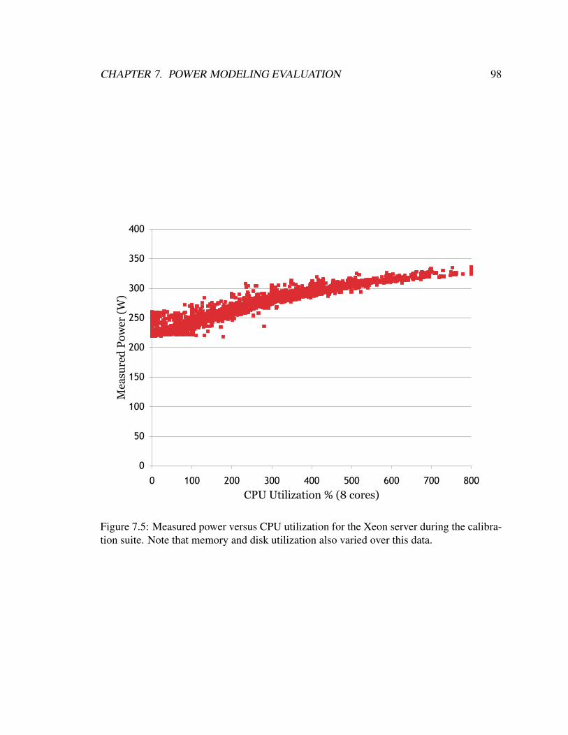
CHAPTER 7. POWER MODELING EVALUATION 98
0
50
100
150
200
250
300
350
400
0 100 200 300 400 500 600 700 800
CPU Utilization % (8 cores)
Me
asu
red
Po
we
r (W
)
Figure 7.5: Measured power versus CPU utilization for the Xeon server during the calibra-tion suite. Note that memory and disk utilization also varied over this data.

CHAPTER 7. POWER MODELING EVALUATION 99
Figure 7.6 shows the mean absolute percentage error for the benchmarks that make
the strongest case for the model based on CPU and disk utilizations. These benchmarks
are the Nsort benchmark and the three CPU-intensive benchmarks, run on CoolSort-13 at
its highest frequency. Since Nsort is the most disk-intensive benchmark, disk utilization
information unsurprisingly improves the power predictions. For the three CPU-intensive
benchmarks, the usefulness of disk utilization information is more surprising, since none
of these benchmarks have significant disk utilization. The reason that the disk information
is helpful is that both the CPU and the disks contribute significantly to the peak dynamic
power of this system, and these two utilizations are not highly correlated. Forcing the
CPU utilization to explain the entire dynamic power variation of the system results in over-
predicting dynamic power when disk utilization is low, particularly for the less flexible
linear model.
Figure 7.7 plots the power predictions of these three models for varying values of CPU
utilization, holding the disk utilization constant at zero. Comparing the predictions at 200%
utilization, the linear model predicts the maximum dynamic power, which is achievable
only with high disk utilization. Both the CPU empirical model and the model that includes
disk utilization predict a lower power consumption that is much closer to the actual dynamic
contribution of the CPU. SPECjbb runs near 200% utilization, and Figure 7.6 accordingly
shows that the linear CPU model yields by far the worst prediction for this benchmark,
while the empirical CPU model and the disk model predict power much more accurately.
At the 100% utilization point, Figure 7.7 shows that the two CPU-utilization-based
models are roughly equivalent and still overpredict power compared to the more accurate
model that uses disk utilization. On this machine, the SPECcpu suite was run on just
one core, corresponding to 100% utilization. As Figure 7.6 shows, the two utilization-
based models predict similar power consumption for the two SPECcpu benchmarks, and

CHAPTER 7. POWER MODELING EVALUATION 100
0
5
10
15
20
25
Nsort SPECfp SPECint SPECjbb
CoolSort-13-hi
Mea
n %
Err
or
Const
CPUut-Lin
CPUut-Emp
CPU+Disk
Perfctr
Figure 7.6: Best case for the CPU- and disk-utilization-based model: Selected benchmarkson CoolSort-13 at the highest frequency.
overpredict compared to the model that includes disk utilization. The example of CoolSort-
13 shows that disk utilization information is useful on systems with high peak dynamic disk
power consumption, even on workloads with very low disk utilization.
Figure 7.8 shows the best case for the performance-counter-based power model. The
leftmost cluster of columns shows the mean absolute percentage error for the stream bench-
mark on the Xeon server, which has 32 GB of FBDIMM memory. Stream is a memory-
intensive but not particularly CPU-intensive benchmark, and so the high dynamic power

CHAPTER 7. POWER MODELING EVALUATION 101
0
20
40
60
80
100
120
0 50 100 150 200
CPU Utilization % (2 cores)
Pre
dic
ted
Po
wer
(W
)
CPUut-Lin
CPUut-Emp
CPU+Disk
Figure 7.7: Power predicted by the CPU-utilization-based models and the CPU and disk-utilization-based model versus CPU utilization on CoolSort-13 at its highest frequency.Disk utilization is assumed to be 0.

CHAPTER 7. POWER MODELING EVALUATION 102
of this machine’s memory is only captured by metrics specifically based on memory uti-
lization. The only model that uses such a metric is the performance-counter-based model,
which includes the performance counter for memory bus transactions as a parameter. This
information results in a much more accurate power prediction.
The other three clusters of columns in Figure 7.8 show the mean absolute percent-
age errors for the models on the CPU-intensive benchmarks on CoolSort-13 at the highest
frequency; this is the same data shown in Figure 7.6 to illustrate the usefulness of disk
utilization. As Figure 7.8 shows, performance counter information further improves the
power predictions for these benchmarks. The reason is that the CPU uses aggressive clock
gating to shut down unused units, even at high utilization [31], so power depends not only
on whether the CPU is utilized, but upon how it is utilized. In particular, the SPECjbb
benchmark has much lower instruction-level parallelism than the SPECcpu benchmarks,
even though it runs on both cores and the SPECcpu benchmarks run on just one.
7.2 Xeon Server Power Models
This section evaluates the power models generated for the Xeon server whose specifications
were given in Section 6.5.2. These models are defined by Equations 7.1 through 7.5. All of
the model inputs are normalized to their maximum values seen during calibration; for the
performance counters, this may not be the maximum possible value. In general, however,
the normalized input values will be between 0 and 1. Therefore, each parameter’s coe!-
cient in the linear models will be equivalent to that parameter’s maximum contribution to
the dynamic power of the system.
In these equations, uCPU and udisk correspond to the CPU and disk utilizations, respec-
tively. The performance counters sampled are unhalted clock cycles (pu), the number of
instructions retired (pi), the number of last-level cache references (pc), and the number

CHAPTER 7. POWER MODELING EVALUATION 103
0
2
4
6
8
10
12
14
16
18
20
Stream SPECfp SPECint SPECjbb
Xeon server CoolSort-13-hi
Mea
n %
Err
or
Const
CPUut-Lin
CPUut-Emp
CPU+Disk
Perfctr
Figure 7.8: Best case for the performance-counter-based model: Selected benchmarks onthe Xeon server and on CoolSort-13 at the highest frequency.

CHAPTER 7. POWER MODELING EVALUATION 104
of memory bus transactions (pm). Note that uCPU and pu should be equivalent; in prac-
tice, however, using both metrics generates more accurate models. For the performance
counter model, the combination of the uCPU and pu terms gives the CPU-utilization-based
contribution to the dynamic power consumption.
Constant model (Equation 7.1).
P = 239.80 (7.1)
Linear CPU-utilization-based model (Equation 7.2).
P = 222.99 + 137.88 ! uCPU
max. uCPU(7.2)
Empirical CPU-utilization-based model (Equation 7.3).
P = 221.08 + 161.71 ! uCPU
max. uCPU# 4.09E-3 !
!uCPU
max. uCPU
"4.55
(7.3)
Linear CPU- and disk-utilization-based model (Equation 7.4).
P = 222.94 + 137.96 ! uCPU
max. uCPU+ 1.96 ! udisk
max. udisk(7.4)
Performance-counter-based model (Equation 7.5).
P = 223.18 # 56.40 ! uCPU
max. uCPU+ 1.60 ! udisk
max. udisk
+ 39.23 ! Pm
max. Pm+ 66.70 ! Pi
max. Pi
+ 27.31 ! Pc
max. Pc+ 95.03 ! Pu
max. Pu(7.5)
Table 7.1 shows the results of the model generation stage. For linear models, the co-
e!cient of determination (R2) is a measure of how much of the deviation from the mean
power consumption is captured by the model parameters. An R2 of 1 means that the model
parameters explain all of the variation in the system’s power consumption. “MSE” is the

CHAPTER 7. POWER MODELING EVALUATION 105
Model R2 MSE Mean Err. % 90th Pct. Err. %Const n/a 585.96 6.93 14.05CPUut-Lin 0.9343 38.49 1.65 3.77CPUut-Emp n/a 22.07 1.32 2.98CPU+Disk 0.9343 38.47 1.64 3.77Perfctr 0.9481 30.40 1.34 3.47
Table 7.1: Model calibration results for the Xeon server.
models’ mean squared error over the calibration data. The remaining two columns list the
mean absolute percentage error and the 90th percentile absolute error for each model. Note
that for the calibration phase, adding more parameters to a model will never increase the
mean squared error; if a particular parameter does not improve the mean squared error, its
coe!cient will be 0 and it will be e"ectively dropped from the model.
Figures 7.9 and 7.10 show the mean and 90th percentile absolute errors, respectively,
for the Mantis-generated models on the Xeon server. The errors are low for the calibra-
tion suite, which is biased toward the idle case, and for ClamAV. As the coe!cient for
disk utilization in Equation 7.4 shows, the disk consumes a very small percentage of the
dynamic power consumption, and so the disk-intensive ClamAV benchmark does not have
high dynamic power consumption either. The stream benchmark results, which were dis-
cussed in Section 7.1, show the necessity of the memory performance counter for memory-
intensive benchmarks on a system with high dynamic memory power. The results of the
CPU-intensive SPEC benchmarks, which were also discussed in Section 7.1, show the use-
fulness of the empirical CPU-utilization-based model for multicore processors with shared
resources.

CHAPTER 7. POWER MODELING EVALUATION 106
0
5
10
15
20
25
calib SPECfp SPECint SPECjbb stream clamAV
Mea
n %
Err
or
Const
CPUut-Lin
CPUut-Emp
CPU+Disk
Perfctr
Figure 7.9: Mean absolute percentage error of the Mantis-generated models on the Xeonserver.
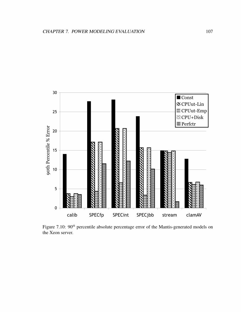
CHAPTER 7. POWER MODELING EVALUATION 107
0
5
10
15
20
25
30
calib SPECfp SPECint SPECjbb stream clamAV
90
th P
erce
nti
le %
Err
or
Const
CPUut-Lin
CPUut-Emp
CPU+Disk
Perfctr
Figure 7.10: 90th percentile absolute percentage error of the Mantis-generated models onthe Xeon server.

CHAPTER 7. POWER MODELING EVALUATION 108
7.3 Itanium Server Power Models
This section evaluates the power models generated for the Itanium server whose specifica-
tions were given in Section 6.5.2. These models are defined by Equations 7.6 through 7.10.
In these equations, uCPU corresponds to the CPU utilization. The performance counters
sampled are L2 cache misses (pl2m), the amount of instruction-level parallelism (pilp), and
the number of floating-point instructions executed (pf ). The Itanium server’s management
processor allows the fan speed to be read; this section therefore includes an additional
model that adds the fan speed (fan) to the performance-counter model. For this server, disk
utilization information did not contribute to the quality of the models, so the “CPU+disk”
model is not present, and the performance counter models do not include disk utilization
information.
Constant model (Equation 7.6).
P = 654.41 (7.6)
Linear CPU-utilization-based model (Equation 7.7).
P = 643.56 + 36.80 ! uCPU
max. uCPU(7.7)
Empirical CPU-utilization-based model (Equation 7.8).
P = 641.11 + 688.45 ! uCPU
max. uCPU# 627.68 !
!uCPU
max. uCPU
"1.04
(7.8)
Performance-counter-based model (Equation 7.9).
P = 622.88 + 25.49 ! uCPU
max. uCPU# 4.12 ! Pf
max. Pf
+ 15.63 ! Pl2m
max. Pl2m+ 31.39 ! Pilp
max. Pilp(7.9)

CHAPTER 7. POWER MODELING EVALUATION 109
Model R2 MSE Mean Err. % 90th Pct. Err. %Const n/a 130.84 1.65 2.18CPUut-Lin 0.7746 29.49 0.63 1.55CPUut-Emp n/a 19.51 0.48 1.07Perfctr 0.8415 20.71 0.49 1.29Perfctr+Fans 0.8417 20.69 0.49 1.29
Table 7.2: Model calibration results for the Itanium server.
Performance-counter-based model plus fan speed (Equation 7.10).
P = 639.37 + 25.43 ! uCPU
max. uCPU# 4.12 ! Pf
max. Pf
+ 15.65 ! Pl2m
max. Pl2m+ 31.53 ! Pilp
max. Pilp
# 16.67 ! fanmax. fan
(7.10)
Table 7.2 shows the results of the model calibration phase on the Itanium server. The R2
values for these models are lower than those for the Xeon server models, indicating that a
higher percentage of this system’s dynamic power is unexplained by the models. Since the
dynamic power on the Itanium is much lower than on the Xeon server, R2 can be a"ected by
a variation of even a few Watts in some unmodeled component, such as the power supply.
Figures 7.11 and 7.12 present the mean and 90th percentile absolute percentage errors,
respectively, for each model over the execution of each benchmark. Note that the “Per-
fctr+Fans” percentage error was always within 0.02 of the “Perfctr” percentage error, so it
is not shown in these graphs. The dynamic power of the fans is di!cult to determine, but
the variation in fan speed over the duration of the benchmarks was low, which may explain
this result.

CHAPTER 7. POWER MODELING EVALUATION 110
Since the dynamic power of this system is so low, all of the models yield much more
accurate predictions than the models for the Xeon server did. The performance-counter-
based model is the most accurate overall, with mean errors of less than 2% for all bench-
marks. The largest disparity between di"erent models occurs for the SPECjbb bench-
mark. SPECjbb, as it did on the Xeon server, has high CPU utilization but relatively low
instruction-level parallelism. Furthermore, this particular server was a prototype whose
operating system did not correctly call the halt instruction when a CPU was idle, which
meant that CPUs did not enter a low-power state when idle. This bug contributed to the
low dynamic power of the system. It also means that CPU utilization is a much less useful
proxy for power, since it does not reflect the percentage of time spent in a low-power state.
As with the Xeon server, how the CPU is utilized becomes important, and the models based
on utilization percentage alone fare poorly on a benchmark that combines high utilization
with low instruction-level parallelism.
Figure 7.11 shows that the constant model actually has the best overall 90th percentile
error; when the dynamic range is low, predicting a power consumption in the middle of the
range will be a consistently safe bet. For the SPECfp, SPECint, and SPECjbb benchmarks,
all of the other models overpredict when the CPU utilization is at its highest point. As with
the Xeon server, shared resource bottlenecks prevent the amount of parallelism from scaling
with utilization. In this system, the bottleneck is the small amount of memory, which
prevents the CPUs from being fully utilized by the SPECcpu and SPECjbb benchmarks.
In conclusion, the constant model easily su!ces for the Itanium system, with its low
dynamic power. However, this system presents a unique platform for understanding the
trade-o"s of the utilization-based models, and shares some qualitative similarities with the
seemingly vastly di"erent Xeon server. The results on both systems suggest that CPU uti-
lization has some limitations as a proxy for power, and that bottlenecks on shared resources
can create a non-linear relationship between utilization and power consumption.

CHAPTER 7. POWER MODELING EVALUATION 111
0
0.5
1
1.5
2
2.5
3
3.5
calib SPECfp SPECint SPECjbb stream SPECweb
Mea
n %
Err
or
Const
CPUut-Lin
CPUut-Emp
Perfctr
Figure 7.11: Mean absolute percentage error of the Mantis-generated models on the Ita-nium server.

CHAPTER 7. POWER MODELING EVALUATION 112
0
1
2
3
4
5
6
7
calib SPECfp SPECint SPECjbb stream SPECweb
90
th P
erce
nti
le %
Err
or
Const
CPUut-Lin
CPUut-Emp
Perfctr
Figure 7.12: 90th percentile absolute percentage error of the Mantis-generated models onthe Itanium server.

CHAPTER 7. POWER MODELING EVALUATION 113
7.4 CoolSort-13 Power Models
This section evaluates the power models generated for the CoolSort 13-disk configuration
(see Section 6.5.2) at its highest processor clock frequency of 2,324 MHz and its lowest
frequency of 996 MHz.
7.4.1 CoolSort-13, Highest Clock Frequency
Equations 7.11 through 7.15 define the models for CoolSort-13 at the highest clock fre-
quency. Refer to Section 7.2 for a discussion of the model inputs used; these models use
the same performance counters as the models for the Xeon server.
Constant model (Equation 7.11).
P = 75.20 (7.11)
Linear CPU-utilization-based model (Equation 7.12).
P = 68.91 + 37.33 ! uCPU
max. uCPU(7.12)
Empirical CPU-utilization-based model (Equation 7.13).
P = 67.12 # 2450 ! uCPU
max. uCPU+ 2490 !
!uCPU
max. uCPU
"0.99
(7.13)
Linear CPU- and disk-utilization-based model (Equation 7.14).
P = 67.86 + 26.55 ! uCPU
max. uCPU+ 18.34 ! udisk
max. udisk(7.14)
Performance-counter-based model (Equation 7.15).
P = 67.74 + 13.97 ! uCPU
max. uCPU+ 20.77 ! udisk
max. udisk
+ 6.20 ! Pm
max. Pm+ 3.33 ! Pi
max. Pi
+ 4.26 ! Pc
max. Pc+ 6.04 ! Pu
max. Pu(7.15)

CHAPTER 7. POWER MODELING EVALUATION 114
Model R2 MSE Mean Err. % 90th Pct. Err. %Const n/a 108.61 11.98 18.52CPUut-Lin 0.5375 50.23 7.43 13.95CPUut-Emp n/a 46.45 6.96 12.92CPU+Disk 0.7210 30.29 5.12 10.57Perfctr 0.7268 29.65 4.99 10.65
Table 7.3: Model calibration results for CoolSort-13 at its highest frequency.
Table 7.3 shows the results of the model generation on CoolSort-13. For this configu-
ration, the linear CPU utilization model has an R2 value of just 0.5375, indicating that just
over half of the dynamic power variation is correlated with CPU utilization. Adding disk
utilization produces much more accurate models, with R2 values above 0.72. The model
coe!cients in Equation 7.14 attribute a dynamic power of 26.55 W to the CPU utiliza-
tion and 18.34 W to the disk utilization. Since CPU and disk utilization are not highly
correlated, both of these quantities are necessary to produce accurate models.
Figures 7.13 and 7.14 show the mean and 90th percentile percentage errors, respectively,
for these models on each benchmark. The performance-counter-based model is the most
accurate model across the board for this system configuration. The results for NSort and the
SPEC benchmarks were discussed in Section 7.1, leaving the stream benchmark. For this
benchmark, the CPU-utilization-based models and the performance-counter-based model
all predict power with comparable accuracy, while the CPU- and disk-utilization-based
model is much less accurate. The reason for its poor performance relative to the models
based on CPU utilization alone is related to the reason that those CPU-utilization-based
models predict SPECjbb’s power so poorly: forced to attribute the entire range of dynamic
power variation to the CPU, the CPU-utilization-based models tend to overpredict power
consumption for a given CPU utilization. The stream benchmark, however, stresses the
memory system, which is not directly captured by CPU or disk utilization. The model
based on CPU and disk utilization does accurately predict CPU and disk power, but does
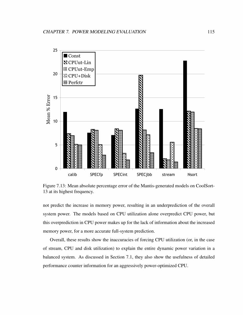
CHAPTER 7. POWER MODELING EVALUATION 115
0
5
10
15
20
25
calib SPECfp SPECint SPECjbb stream Nsort
Mea
n %
Err
or
Const
CPUut-Lin
CPUut-Emp
CPU+Disk
Perfctr
Figure 7.13: Mean absolute percentage error of the Mantis-generated models on CoolSort-13 at its highest frequency.
not predict the increase in memory power, resulting in an underprediction of the overall
system power. The models based on CPU utilization alone overpredict CPU power, but
this overprediction in CPU power makes up for the lack of information about the increased
memory power, for a more accurate full-system prediction.
Overall, these results show the inaccuracies of forcing CPU utilization (or, in the case
of stream, CPU and disk utilization) to explain the entire dynamic power variation in a
balanced system. As discussed in Section 7.1, they also show the usefulness of detailed
performance counter information for an aggressively power-optimized CPU.

CHAPTER 7. POWER MODELING EVALUATION 116
0
5
10
15
20
25
30
calib SPECfp SPECint SPECjbb stream Nsort
90
th P
erce
nti
le %
Err
or
Const
CPUut-Lin
CPUut-Emp
CPU+Disk
Perfctr
Figure 7.14: 90th percentile absolute percentage error of the Mantis-generated models onCoolSort-13 at its highest frequency.

CHAPTER 7. POWER MODELING EVALUATION 117
7.4.2 CoolSort-13, Lowest Clock Frequency
Equations 7.16 through 7.20 define the models for CoolSort-13 at its lowest clock fre-
quency, 996 MHz. Refer to Section 7.2 for a discussion of the model inputs used. This
configuration has perhaps the most unusual component balance seen in this study: with the
CPU at its lowest frequency, its dynamic power is dwarfed by the disk’s dynamic power
and is lower than the memory’s dynamic power. For this reason, the performance counter
model uses only the cache and memory performance counters to represent CPU and mem-
ory power. Because interfaces for obtaining hardware information from the memory and
disk are not at the level of detail of CPU performance counters, the models for this system
are the least accurate overall, as shown in Table 7.4.
Constant model (Equation 7.16).
P = 67.21 (7.16)
Linear CPU-utilization-based model (Equation 7.17).
P = 62.93 + 17.53 ! uCPU
max. uCPU(7.17)
Empirical CPU-utilization-based model (Equation 7.18).
P = 62.59 # 2461 ! uCPU
max. uCPU+ 2479 !
!uCPU
max. uCPU
"0.999
(7.18)
Linear CPU- and disk-utilization-based model (Equation 7.19).
P = 62.60 + 7.61 ! uCPU
max. uCPU+ 22.13 ! udisk
max. udisk(7.19)
Performance-counter-based model (Equation 7.20).
P = 62.59 + 25.88 ! udisk
max. udisk+ 6.21 ! Pm
max. Pm
+ 5.55 ! Pc
max. Pc(7.20)

CHAPTER 7. POWER MODELING EVALUATION 118
Model R2 MSE Mean Err. % 90th Pct. Err. %Const n/a 61.31 9.35 15.14CPUut-Lin 0.3746 38.34 7.14 14.35CPUut-Emp n/a 38.25 7.13 14.55CPU+Disk 0.6364 22.28 5.01 9.30Perfctr 0.6411 22.00 4.78 9.53
Table 7.4: Model calibration results for CoolSort-13 at its lowest frequency.
Figures 7.15 and 7.16 show the mean and 90th percentile percentage errors for the dif-
ferent models on each benchmark run on this system. The CPU-utilization-based models
are clearly worst, since they attribute the entire dynamic power variation of the system to
the component with the least dynamic variation. The performance-counter-based model
does best in general, since it has some information about the memory subsystem. The re-
sults for the stream benchmark are due to the e"ect described in Section 7.4.1, and have
to do with the fact that the performance counter model is the only one with access to
memory information. Once again, the CPU+disk model underpredicts the total system
power, and the CPU-utilization-based models slightly overpredict. In this case, however,
the CPU-utilization-based models’ overprediction comes quite close to the actual power
consumption. Overall, this configuration shows the di!culty of developing power models
for systems where the CPU does not dominate the dynamic power. One reason for this
di!culty is the lack of detailed memory and disk metrics that help model dynamic power
consumption.
7.5 CoolSort-1 Power Models
This section evaluates the power models generated for the CoolSort single-disk configu-
ration (see Section 6.5.2) at its highest processor clock frequency of 2,324 MHz and its
lowest frequency of 996 MHz.

CHAPTER 7. POWER MODELING EVALUATION 119
0
5
10
15
20
25
calib SPECfp SPECint SPECjbb stream Nsort
Mea
n %
Err
or
Const
CPUut-Lin
CPUut-Emp
CPU+Disk
Perfctr
Figure 7.15: Mean absolute percentage error of the Mantis-generated models on CoolSort-13 at its lowest frequency.

CHAPTER 7. POWER MODELING EVALUATION 120
0
5
10
15
20
25
30
calib SPECfp SPECint SPECjbb stream Nsort
90
th P
erce
nti
le %
Err
or
Const
CPUut-Lin
CPUut-Emp
CPU+Disk
Perfctr
Figure 7.16: 90th percentile absolute percentage error of the Mantis-generated models onCoolSort-13 at its lowest frequency.

CHAPTER 7. POWER MODELING EVALUATION 121
7.5.1 CoolSort-1, Highest Clock Frequency
Equations 7.21 through 7.25 define the models for CoolSort-1 at its highest clock fre-
quency. Refer to Section 7.2 for a discussion of the model inputs used; these models use
the same performance counters as the models for the Xeon server. Table 7.5 shows the
results of fitting these equations to the calibration data.
With just one disk and running at its highest clock frequency, CoolSort-1’s dynamic
power consumption is dominated by the processor and secondarily by memory. The disk
power becomes insignificant, as the coe!cients for disk utilization in Equations 7.24
and 7.25 show. With CPU as the dominant component of dynamic power consumption, the
models developed for this system are highly accurate, with R2 values similar to those for
the CPU- and memory-dominated Xeon server.
Constant model (Equation 7.21).
P = 56.59 (7.21)
Linear CPU-utilization-based model (Equation 7.22).
P = 52.78 + 33.16 ! uCPU
max. uCPU(7.22)
Empirical CPU-utilization-based model (Equation 7.23).
P = 52.48 + 37.40 ! uCPU
max. uCPU# 0.79 !
!uCPU
max. uCPU
"5.00
(7.23)
Linear CPU- and disk-utilization-based model (Equation 7.24).
P = 52.81 + 33.13 ! uCPU
max. uCPU# 0.13 ! udisk
max. udisk(7.24)

CHAPTER 7. POWER MODELING EVALUATION 122
Model R2 MSE Mean Err. % 90th Pct. Err. %Const n/a 42.80 7.61 20.07CPUut-Lin 0.8783 5.20 1.85 4.20CPUut-Emp n/a 4.10 1.56 3.03CPU+Disk 0.8783 5.21 1.87 4.20Perfctr 0.9146 3.65 1.41 2.17
Table 7.5: Model calibration results for CoolSort-1 at its highest frequency.
Performance-counter-based model (Equation 7.25).
P = 52.71 + 29.50 ! uCPU
max. uCPU+ 1.61 ! udisk
max. udisk
+ 11.70 ! Pm
max. Pm+ 16.21 ! Pi
max. Pi
# 36.93 ! Pc
max. Pc+ 13.40 ! Pu
max. Pu(7.25)
Figures 7.17 and 7.18 show the mean and 90th percentile percentage errors, respec-
tively, for CoolSort-1 at its highest frequency. All of the models that use utilization in-
formation significantly outperform the constant power model. The only benchmark for
which any of these models predicts inaccurately is SPECjbb, for which the linear CPU and
CPU+disk models have mean errors of over 10%. These results are qualitatively similar
to the SPECjbb results on the Xeon server, described in Section 7.1, for the same reason:
SPECjbb combines high CPU utilization with relatively low instruction-level parallelism.
On this aggressively power-managed processor, as discussed in Section 7.4, clock gating is
used to reduce the power consumption of unused parts of the processor. Therefore, detailed
information about how the processor is being utilized is necessary to make accurate power
predictions.

CHAPTER 7. POWER MODELING EVALUATION 123
0
5
10
15
20
25
calib SPECfp SPECint SPECjbb stream clamAV
Mea
n %
Err
or
Const
CPUut-Lin
CPUut-Emp
CPU+Disk
Perfctr
Figure 7.17: Mean absolute percentage error of the Mantis-generated models on CoolSort-1 at its highest frequency.

CHAPTER 7. POWER MODELING EVALUATION 124
0
5
10
15
20
25
calib SPECfp SPECint SPECjbb stream clamAV
90
th P
erce
nti
le %
Err
or
Const
CPUut-Lin
CPUut-Emp
CPU+Disk
Perfctr
Figure 7.18: 90th percentile absolute percentage error of the Mantis-generated models onCoolSort-1 at its highest frequency.

CHAPTER 7. POWER MODELING EVALUATION 125
7.5.2 CoolSort-1, Lowest Clock Frequency
Equations 7.26 through 7.30 define the models for CoolSort-1 at its lowest clock frequency.
Refer to Section 7.2 for a discussion of the model inputs used; these models use the same
performance counters as the models for the Xeon server. Table 7.6 shows the results of
fitting these equations to the calibration data.
Figures 7.19 and 7.20 show the mean and 90th percentile percentage errors, respec-
tively, of the models on this configuration. With just one disk and running at its lowest
clock frequency, CoolSort-1’s dynamic power consumption is dominated by the proces-
sor and memory. The results are qualitatively similar to the results for CoolSort-1 at the
highest frequency (Section 7.5.1), with a few di"erences. First, since the memory is a pro-
portionally higher consumer of dynamic power when the processor frequency is low, the
performance counter model now predicts power with a much lower percentage error for the
memory-intensive stream benchmark. Secondly, now that the processor has a lower share
of the dynamic power consumptions, the CPU-utilization-based models contain some in-
accuracies from having to attribute all of the system’s dynamic power to the processor, as
their overpredictions for the SPEC CPU benchmarks show.
Constant model (Equation 7.26).
P = 50.08 (7.26)
Linear CPU-utilization-based model (Equation 7.27).
P = 48.44 + 10.65 ! uCPU
max. uCPU(7.27)
Empirical CPU-utilization-based model (Equation 7.28).
P = 48.08 + 14.58 ! uCPU
max. uCPU# 0.69 !
!uCPU
max. uCPU
"4.57
(7.28)

CHAPTER 7. POWER MODELING EVALUATION 126
Model R2 MSE Mean Err. % 90th Pct. Err. %Const n/a 7.59 3.94 10.57CPUut-Lin 0.6785 2.44 2.03 5.18CPUut-Emp n/a 1.68 1.67 3.37CPU+Disk 0.6806 2.42 1.96 5.28Perfctr 0.8756 0.94 1.14 2.05
Table 7.6: Model calibration results for CoolSort-1 at its lowest frequency.
Linear CPU- and disk-utilization-based model (Equation 7.29).
P = 48.35 + 10.71 ! uCPU
max. uCPU+ 0.34 ! udisk
max. udisk(7.29)
Performance-counter-based model (Equation 7.30).
P = 48.15 + 5.09 ! uCPU
max. uCPU+ 1.44 ! udisk
max. udisk
+ 7.01 ! Pm
max. Pm+ 5.52 ! Pi
max. Pi
# 5.19 ! Pc
max. Pc+ 3.48 ! Pu
max. Pu(7.30)
7.6 Laptop Power Models
The final machine on which the Mantis models were evaluated is a 2005-era laptop with
an AMD processor. Section 7.6.1 shows the results for this processor’s highest frequency,
1,800 MHz, and Section 7.6.2 shows the results for its lowest frequency, 800 MHz.
For this processor, we were unable to use any main memory-related performance coun-
ters. The “memory requests” performance counter is not analogous to the “memory bus
transactions” performance counter on the Intel processors studied in this chapter. Memory
power is related to the actual memory tra!c, which “memory bus transactions” captures.

CHAPTER 7. POWER MODELING EVALUATION 127
0
2
4
6
8
10
12
14
16
clam SPECfp SPECint SPECjbb stream clamAV
Mea
n %
Err
or
Const
Goog-Lin
Goog-Emp
Heath
Zesti
Figure 7.19: Mean absolute percentage error of the Mantis-generated models on CoolSort-1 at its lowest frequency.

CHAPTER 7. POWER MODELING EVALUATION 128
0
2
4
6
8
10
12
14
16
clam SPECfp SPECint SPECjbb stream clamAV
90
th P
erce
nti
le %
Err
or
Const
Goog-Lin
Goog-Emp
Heath
Zesti
Figure 7.20: 90th percentile absolute percentage error of the Mantis-generated models onCoolSort-1 at its lowest frequency.

CHAPTER 7. POWER MODELING EVALUATION 129
“Memory requests,” however, only captures the requests that the processor is aware of mak-
ing, which means that it will undercount the memory tra!c for memory-intensive bench-
marks with predictable access patterns that are handled by the prefetcher. For this system,
a power model using “memory requests” was generated using the calibration suite, which
stresses memory with predictable access patterns. For the irregular accesses in the gcc
benchmark, however, the model proved disastrous, as the number of “memory requests”
far exceeded anything seen in the calibration data. We therefore dropped this model pa-
rameter. Attempting to instead use the performance counter for DRAM pages accessed re-
sulted in unacceptably high overhead in the performance-counting software, so ultimately
the only performance counters used were unhalted clock cycles (pu), floating-point instruc-
tions dispatched (pf ), and number of instructions retired (pi). The number of last-level
cache references did not improve the model as much as these three counters, and so it was
not used in the models.
7.6.1 Laptop, Highest Clock Frequency
Equations 7.31 through 7.35 define the models for the laptop at its highest frequency. The
dynamic power variation for this configuration is dominated by the CPU, as the coe!-
cients of Equations 7.34 and 7.35 show. As with the other CPU-dominated systems, the R2
goodness-of-fit values are high (above 0.8), as shown in Table 7.7.
Figures 7.21 and 7.22 show the mean and 90th percentile percentage errors, respectively,
for each benchmark on this system. Note that the gcc benchmark is used rather than the
entire SPECint suite, and that gromacs is used instead of the entire SPECfp suite, due to the
limited resources on this system. All of the models significantly outperform the constant
prediction; overall, the best model is the linear CPU utilization model. Lacking information
about the memory subsystem, the performance counter model no longer excels at predicting
power for stream. Because of the limitations of this system’s processor, SPECjbb is a

CHAPTER 7. POWER MODELING EVALUATION 130
much more CPU- and memory-intensive benchmark than on the other machines, which is
underpredicted by the CPU+disk and performance-counter-based models. ClamAV is the
hardest test case for the models overall, as they all overpredict the power consumption at
this medium level of CPU utilization (60%).
Constant model (Equation 7.31).
P = 25.94 (7.31)
Linear CPU-utilization-based model (Equation 7.32).
P = 20.73 + 17.56 ! uCPU
max. uCPU(7.32)
Empirical CPU-utilization-based model (Equation 7.33).
P = 19.09 + 61.1 ! uCPU
max. uCPU# 42.76 !
!uCPU
max. uCPU
"1.22
(7.33)
Linear CPU- and disk-utilization-based model (Equation 7.34).
P = 19.39 + 16.81 ! uCPU
max. uCPU+ 3.70 ! udisk
max. udisk(7.34)
Performance-counter-based model (Equation 7.35).
P = 13.24 + ! uCPU
max. uCPU+ 2.48 ! udisk
max. udisk
+ 3.139 ! Pu
max. Pu+ 2.51 ! Pf
max. Pf
+ 3.37 ! Pi
max. Pi(7.35)

CHAPTER 7. POWER MODELING EVALUATION 131
Model R2 MSE Mean Err. % 90th Pct. Err. %Const n/a 46.14 22.17 39.49CPUut-Lin 0.8365 7.54 8.65 15.50CPUut-Emp n/a 6.17 6.68 13.78CPU+Disk 0.8933 4.92 5.47 11.53Perfctr 0.8962 4.79 5.36 11.44
Table 7.7: Model calibration results for the laptop at its highest frequency.
0
5
10
15
20
25
30
35
calib gromacs gcc SPECjbb stream clamAV
Mea
n %
Err
or
Const
CPUut-Lin
CPUut-Emp
CPU+Disk
Perfctr
Figure 7.21: Mean absolute percentage error of the Mantis-generated models on the laptopat its highest frequency.

CHAPTER 7. POWER MODELING EVALUATION 132
0
5
10
15
20
25
30
35
40
calib gromacs gcc SPECjbb stream clamAV
90
th P
erce
nti
le %
Err
or
Const
CPUut-Lin
CPUut-Emp
CPU+Disk
Perfctr
Figure 7.22: 90th percentile absolute percentage error of the Mantis-generated models onthe laptop at its highest frequency.

CHAPTER 7. POWER MODELING EVALUATION 133
7.6.2 Laptop, Lowest Clock Frequency
Equations 7.36 through 7.40 define the models for the laptop at its highest frequency. This
configuration has much lower dynamic power consumption than the high-frequency con-
figuration, as the coe!cients of Equations 7.39 and 7.40 show. Since the CPU is a less
dominant consumer of dynamic power, the R2 goodness-of-fit values are also lower than in
the high-frequency configuration, as shown in Table 7.8.
Figures 7.23 and 7.24 show the mean and 90th percentile percentage errors, respectively,
for each benchmark on this system. The main di"erences between this configuration and
the high-frequency configuration are in the clamAV benchmark, where the overpredictions
for this configuration are slightly lower, and in the gromacs floating-point benchmark. For
gromacs, all of the models now overpredict power. The reason is that gromacs thoroughly
stresses this CPU in terms of both utilization and instruction-level parallelism. However,
it is largely resident in cache and does not stress the memory subsystem as thoroughly.
Since none of the models have memory information, they are all forced to attribute the en-
tire dynamic power to CPU utilization characteristics, significantly overpredicting the total
power when the CPU is the only highly utilized component. This is particularly problem-
atic at this low frequency, since the CPU is a proportionately smaller consumer of the total
dynamic power.
Constant model (Equation 7.36).
P = 15.98 (7.36)
Linear CPU-utilization-based model (Equation 7.37).
P = 14.33 + 5.33 ! uCPU
max. uCPU(7.37)
Empirical CPU-utilization-based model (Equation 7.38).
P = 14.25 + 6.13 ! uCPU
max. uCPU# 0.78 !
!uCPU
max. uCPU
"1.63
(7.38)

CHAPTER 7. POWER MODELING EVALUATION 134
Model R2 MSE Mean Err. % 90th Pct. Err. %Const n/a 4.33 10.09 19.48CPUut-Lin 0.7863 0.93 4.11 7.99CPUut-Emp n/a 0.92 4.04 7.95CPU+Disk 0.8152 0.80 3.34 7.12Perfctr 0.8272 0.75 3.20 6.41
Table 7.8: Model calibration results for the laptop at its lowest frequency.
Linear CPU- and disk-utilization-based model (Equation 7.39).
P = 14.05 + 5.46 ! uCPU
max. uCPU+ 0.91 ! udisk
max. udisk(7.39)
Performance-counter-based model (Equation 7.40).
P = 13.96 + 3.33 ! uCPU
max. uCPU+ 0.67 ! udisk
max. udisk
+ 2.80 ! Pu
max. Pu+ 0.26 ! Pf
max. Pf
# 2.61 ! Pi
max. Pi(7.40)
7.7 Conclusions
The results presented in this section show that simple, high-level models can be used to
accurately predict power for a wide range of systems and workloads. They also highlight
some potential pitfalls in developing power models:
• CPU utilization as a proxy for power consumption. CPU utilization is often con-
sidered a first-order proxy for dynamic power consumption, the logic being that
the CPU is the dominant consumer of dynamic power and that its power is deter-
mined largely by its power state (active or sleeping). For systems that are not CPU-
dominated (e.g. fileservers, some laptops) or workloads that are not CPU-intensive

CHAPTER 7. POWER MODELING EVALUATION 135
0
5
10
15
20
25
calib gromacs gcc SPECjbb stream clamAV
Mea
n %
Err
or
Const
CPUut-Lin
CPUut-Emp
CPU+Disk
Perfctr
Figure 7.23: Mean absolute percentage error of the Mantis-generated models on the laptopat its lowest frequency.

CHAPTER 7. POWER MODELING EVALUATION 136
0
5
10
15
20
25
calib gromacs gcc SPECjbb stream clamAV
90
th P
erce
nti
le %
Err
or
Const
CPUut-Lin
CPUut-Emp
CPU+Disk
Perfctr
Figure 7.24: 90th percentile absolute percentage error of the Mantis-generated models onthe laptop at its lowest frequency.

CHAPTER 7. POWER MODELING EVALUATION 137
(e.g. streaming, sorting), these assumptions break down. They also break down in
two situations, even for systems and workloads that are CPU-dominated. The first is
in processors with shared resources, such as multicore processors, where power con-
sumption is not a linear function of utilization. The second is in aggressively power-
managed processors, where the active-state power consumption may vary widely
depending on what the CPU is actually doing. Since current hardware trends are to-
ward less CPU-dominated systems [5], multicore processors, and aggressive power
management, OS-reported CPU utilization will be a less and less useful proxy for
power consumption.
• Assuming that more information yields a better model. If a large component of
the system’s dynamic power is not directly accounted for by the power models, less
detailed models may actually yield better results, as seen with the stream benchmark
on CoolSort-13. In general, models’ relative accuracy will be unpredictable if a large
component of dynamic power is not modeled.
• Blindly applying performance counters across systems. While the same basic
group of performance counters (unhalted clock cycles, instructions retired/ILP, last-
level cache references, memory bandwidth, and floating-point instructions executed)
can be used to model power across a wide variety of systems, the nuances of how
these counters are defined from platform to platform do matter. To yield an accurate
model, a performance event must be represented over its entire range in the calibra-
tion suite. With the laptop’s AMD processor, the distinction between AMD’s “mem-
ory requests” performance counter and Intel’s “memory bus transactions” counter
became clear: the former was not well exercised during the calibration suite, due to
its predictable access patterns, and so it did not yield accurate models.
• Lack of insight into memory and disk power. Systems that were CPU-dominated
resulted in more accurate models than systems dominated by other components.

CHAPTER 7. POWER MODELING EVALUATION 138
While some have argued that CPU manufacturers should implement event coun-
ters for energy-related events [34], the current CPU performance counters do give
some insight into power consumption. Similar high-level interfaces do not exist for
memory and disk, limiting the accuracy of this approach for systems where those
components are dominant consumers of power. This problem is likely to increase in
the future, since CPUs’ percentage of overall system power is decreasing [5].
In general, across the wide variety of systems tested, the performance-counter-based
power model we proposed met our accuracy requirements on all benchmarks and was gen-
eral enough to be easily portable across systems. For some systems, simpler approaches
may be just as good. The Mantis modeling methodology allows an entire family of models
to easily be developed, and their trade-o"s evaluated, for a wide range of computer systems.

Chapter 8
Conclusions
139

CHAPTER 8. CONCLUSIONS 140
This dissertation examined the question of how to provide widely applicable models and
metrics for energy-e!cient computer systems. It presented the specification for JouleSort,
the first complete full-system energy-e!ciency benchmark to be proposed, and it described
the Mantis methodology for generating and evaluating a family of high-level, full-system
power models.
JouleSort was the first full-system energy-e!ciency benchmark with fully specified
workload, metric, and rules. This dissertation presented the complete benchmark spec-
ification, highlighting the challenges and pitfalls of energy-e!ciency benchmarking that
distinguish it from benchmarking pure performance. It also evaluated the JouleSort bench-
mark scores of a number of systems, including previous generations of high-performing
and highly cost-e!cient sorting systems as well as current commodity machines. These
evaluations motivated the design of the CoolSort system, the machine with the highest
known JouleSort score. This machine, consisting of a commodity mobile CPU and 13 lap-
top drives connected by server-style I/O interfaces, di"ers greatly from today’s commer-
cially available servers. It remains a high-scoring system for metrics using several di"erent
combinations of cost, performance, and power.
Mantis generates full-system power models by correlating AC power measurements
with software utilization metrics. This dissertation evaluated several di"erent families of
Mantis-generated models on several computer systems with widely varying components
and power footprints, identifying models that are both highly accurate and highly portable.
This evaluation demonstrates the trade-o" between simplicity and accuracy, and it also
shows the limitations of previously proposed models based solely on OS-reported compo-
nent utilization for systems where the CPU is either aggressively power-managed or is not
the dominant consumer of dynamic power. Given hardware trends in exactly these direc-
tions, these models will be increasingly inadequate in the future, and the specific modeling
strategy we proposed that uses both OS-reported utilization and CPU performance counters
will be increasingly necessary for accurate power prediction.

CHAPTER 8. CONCLUSIONS 141
8.1 Future Work
Metrics and models for energy-e!cient computing have only recently begun to receive
systematic attention. The JouleSort and Mantis work described in this dissertation leaves
some questions unaddressed and suggests some possible extensions to cover a wider range
of systems.
• In designing the CoolSort system for the JouleSort benchmark, we focused primarily
on the 100 GB benchmark class. The most energy-e!cient systems for the 10 GB
and 1 TB benchmark classes may be constructed very di"erently from CoolSort’s
mobile fileserver design. At the 10 GB class, ultra-low-power components and flash
drives are promising technologies, although the question of how best to connect them
remains open [58]. For the 1 TB class, a more traditional category of server may be
best. The Sun UltraSPARC T1 and T2 processor designs, which maximize memory
bandwidth and thread-level parallelism at the cost of processor complexity that is
largely unneeded by sort, seem ideal as sorting processors [44]. The question of how
to build an energy-e!cient sorting system around such a processor, and what class
of components to use, has yet to be explored.
• The JouleSort benchmark does not address every possible domain of interest for en-
ergy e!ciency. The workload is I/O-intensive, making it a less useful benchmark in
situations where I/O bandwidth is not important. It also allows systems to run at their
most energy-e!cient operating point, which is currently peak utilization. However,
many data center and server machines are underutilized [5]. The SPECpower ssj
benchmark addresses this area to some extent, but its CPU- and memory-intensive
workload is very di"erent from JouleSort’s; in addition, it summarizes energy e!-
ciency at ten di"erent operating points with one number, meaning that the energy
e!ciency at any particular utilization is unclear from the benchmark score. Finally,
JouleSort is not a data-center-level benchmark, since it does not include power and

CHAPTER 8. CONCLUSIONS 142
cooling; developing a fair workload, metric, and rules for a building-scale energy-
e!ciency computing benchmark is a challenge that has yet to be addressed.
• The models investigated in this work were very simple, not only in the number of
inputs sampled, but also in the complexity of the equations used to obtain power pre-
dictions from utilization metrics. As Chapter 7 showed, these simple, mostly linear
models may not adequately express the behavior of some systems, multicores in par-
ticular. Combining the empirical power model for CPU power with the information
provided by disk utilization and CPU performance counters is one obvious extension.
• The models we investigated assume that the dynamic power correlates to the utiliza-
tion of CPU, memory, and disk. Systems with other components, such as graphics
processors or power-aware networking equipment, will require adjustments to the
calibration suite. Furthermore, future power optimizations are likely to pose model-
ing challenges: in particular, the dynamic power consumption of the cooling system
and aggressive power-management policies in individual components would have to
be visible to the OS and incorporated in the model.
• As Chapter 7 showed, power models are less accurate for machines whose dynamic
power consumption is not CPU-dominated. Since the CPU is likely to be a less
dominant component in the future [5], it is important to understand how to develop
accurate power models for other components. Part of the solution may be to o"er
high-level interfaces to detailed metrics for these components, analogous to CPU
performance counters and their interface libraries.
• Finally, while several of the models evaluated in Chapter 7 have been employed in
data center energy-e!ciency optimizations, the performance counter-based model

CHAPTER 8. CONCLUSIONS 143
has not yet been incorporated into a data center scheduler. Evaluating it in this con-
text would help to quantify the energy-e!ciency improvements of increased model
accuracy.

Bibliography
[1] Anonymous. A measure of transaction processing performance. Datamation,
31(7):112–118, April 1985.
[2] ASHRAE handbook. Online. http://resourcecenter.ashrae.org/store/
ashrae/newstore.cgi?categoryid=146.
[3] Reza Azimi, Michael Stumm, and Robert W. Wizniewski. Online performance anal-
ysis by statistical sampling of microprocessor performance counters. In Proceedings
of the International Conference on Supercomputing (ICS), June 2005.
[4] Luiz Andre Barroso. The price of performance. ACM Queue, 3(7):48–53, September
2005.
[5] Luiz Andre Barroso and Urs Holzle. The case for energy-proportional computing.
IEEE Computer, 40(12):33–37, December 2007.
[6] Frank Bellosa. The benefits of event-driven energy accounting in power-sensitive
systems. In Proceedings of the ACM SIGOPS European Workshop, June 2000.
[7] Pradip Bose. Power-e!cient microarchitectural choices at the early definition stage.
Keynote address at the Workshop on Power-Aware Computer Systems (PACS), De-
cember 2003.
144

BIBLIOGRAPHY 145
[8] David Brooks, Vivek Tiwari, and Margaret Martonosi. Wattch: A framework for
architectural-level power analysis and optimizations. In Proceedings of the Interna-
tional Symposium on Computer Architecture (ISCA), June 2000.
[9] Doug Burger and Todd M. Austin. The SimpleScalar tool set, version 2.0. ACM
SIGARCH Computer Architecture News, 25(3):13–25, June 1997.
[10] Todd L. Cignetti, Kirill Komarov, and Carla Schlatter Ellis. Energy estimation tools
for the PalmT M. In Proceedings of the International Workshop on Modeling, Analysis
and Simulation of Wireless and Mobile Systems, 2000.
[11] Clam AntiVirus. Online. http://www.clamav.net/.
[12] Gilberto Contreras and Margaret Martonosi. Power prediction for Intel XScale® pro-
cessors using performance monitoring unit events. In Proceedings of the International
Symposium on Low-Power Electronics and Design (ISLPED), August 2005.
[13] Je"rey Dean and Sanjay Ghemawat. MapReduce: Simplified data processing on large
clusters. In Proceedings of the USENIX Symposium on Operating System Design and
Implementation (OSDI), December 2004.
[14] Dimitris Economou, Suzanne Rivoire, et al. Full-system power analysis and modeling
for server environments. In Proceedings of the Workshop on Modeling, Benchmark-
ing, and Simulation (MoBS), June 2006.
[15] The Embedded Microprocessor Benchmark Consortium (EEMBC). Online. http:
//www.eembc.org.
[16] The Embedded Microprocessor Benchmark Consortium (EEMBC). Energy-
Bench™ version 1.0 power/energy benchmarks. Online. http://www.eembc.org/
benchmark/power_sl.php.

BIBLIOGRAPHY 146
[17] Energy Star program requirements for computers: Version 4.0. On-
line, 2007. http://www.energystar.gov/ia/partners/prod_development/
revisions/downloads/computer/Computer_Spec_Final.pdf.
[18] Xiaobo Fan, Wolf-Dietrich Weber, and Luiz Andre Barroso. Power provisioning for a
warehouse-sized computer. In Proceedings of the International Symposium on Com-
puter Architecture (ISCA), June 2007.
[19] Wes Felter, Karthick Rajamani, et al. A performance-conserving approach for reduc-
ing peak power consumption in server systems. In Proceedings of the International
Conference on Supercomputing (ICS), June 2005.
[20] Ricardo Gonzalez and Mark Horowitz. Energy dissipation in general purpose mi-
croprocessors. IEEE Journal of Solid-State Circuits, 31(9):1277–1284, September
1996.
[21] Naga Govindaraju, Jim Gray, et al. GPUTeraSort: High performance graphics copro-
cessor sorting for large database management. In SIGMOD Conference on Manage-
ment of Data, June 2006.
[22] The Green Grid. The Green Grid data center power e!ciency metrics: PUE and
DCiE. Online, 2007. http://www.thegreengrid.org/gg_content/TGG_Data_
Center_Power_Efficiency_Metrics_PUE_and_DCiE.pdf.
[23] The Green Grid. The Green Grid opportunity: Decreasing datacenter and other
IT energy usage patterns. Online, 2007. http://www.thegreengrid.org/gg_
content/Green_Grid_Position_WP.pdf.
[24] The Green Grid. A framework for data center energy productivity. Online, 2008.
http://www.thegreengrid.org/home/White_Paper_13_-_Framework_for_
Data_Center_Energy_Productivity5.9.08.pdf.

BIBLIOGRAPHY 147
[25] Sudhanva Gurumurthi, Anand Sivasubramaniam, et al. Using complete machine sim-
ulation for software power estimation: the SoftWatt approach. In Proceedings of
the International Symposium on High-Performance Computer Architecture (HPCA),
February 2002.
[26] Taliver Heath, Ana Paula Centeno, et al. Mercury and Freon: temperature emulation
and management for server systems. In Proceedings of the International Confer-
ence on Architectural Support for Programming Languages and Operating Systems
(ASPLOS), October 2006.
[27] Taliver Heath, Bruno Diniz, et al. Energy conservation in heterogeneous server clus-
ters. In Proceedings of the Symposium on Principles and Practice of Parallel Pro-
gramming (PPoPP), June 2005.
[28] HP Enterprise Configurator power calculators. Online, October 2006. http:
//h30099.ww3.hp.com/configurator/powercalcs.asp.
[29] Hitachi Travelstar 5K160 datasheet. Online. http://www.hitachigst.com/hdd/
support/5k160/5k160.htm.
[30] Xing Huang, Bo Huang, and Binheng Song. Bytes-split-index sort (BSIS).
Online, 2006. http://research.microsoft.com/barc/SortBenchmark/
BSIS-PennySort_2006.pdf.
[31] Intel® Core™ 2 Duo mobile processor product brief. Online. http://www.intel.
com/products/processor/core2duo/mobile_prod_brief.htm.
[32] Canturk Isci and Margaret Martonosi. Runtime power monitoring in high-end pro-
cessors: Methodology and empirical data. In Proceedings of the International Sym-
posium on Microarchitecture (MICRO-36), December 2003.

BIBLIOGRAPHY 148
[33] Russ Joseph and Margaret Martonosi. Run-time power estimation in high perfor-
mance microprocessors. In Proceedings of the International Symposium on Low-
Power Electronics and Design (ISLPED), August 2001.
[34] Ismail Kadayif, T. Chinoda, et al. vEC: Virtual energy counters. In Proceedings of
the ACM SIGPLAN/SIGSOFT Workshop on Program Analysis for Software Tools and
Engineering (PASTE), June 2001.
[35] Kingston memory module specification: KVR667D2N5/1G. Online. http://www.
valueram.com/datasheets/KVR667D2N5_1G.pdf.
[36] Ramakrishna Kotla, Anirudh Devgan, et al. Characterizing the impact of di"erent
memory-intensity levels. In Proceedings of the IEEE Annual Workshop on Workload
Characterization (WWC-7), October 2004.
[37] James Laudon. Performance/Watt: the new server focus. SIGARCH Computer Ar-
chitecture News, 33(4):5–13, November 2005.
[38] Tao Li and Lizy Kurian John. Run-time modeling and estimation of operating sys-
tem power consumption. In Proceedings of the ACM SIGMETRICS International
Conference on Measurement and Modeling of Computer Systems, June 2003.
[39] M. R. Lindeburg. Mechanical Engineering Reference Manual. Professional Publica-
tions, tenth edition, 1997.
[40] Peter Lyman, Hal R. Varian, et al. How much information? Online, 2003. http:
//www2.sims.berkeley.edu/research/projects/how-much-info-2003/.
[41] Christopher Malone and Christian Belady. Metrics and an infrastructure model to
evaluate data center e!ciency. In Proceedings of the Pacific Rim/ASME International
Electronic Packaging Technical Conference and Exhibition (IPACK), July 2007.

BIBLIOGRAPHY 149
[42] John Marko" and Saul Hansell. Hiding in plain sight, Google seeks more power. New
York Times, Jun. 14, 2006.
[43] John D. McCalpin. STREAM: Sustainable memory bandwidth in high performance
computers. Online. http://www.cs.virginia.edu/stream/.
[44] Harlan McGhan. Niagara 2 opens the floodgates: Niagara 2 is the closest thing yet to
a true server on a chip. Microprocessor Report, Nov. 1, 2006.
[45] Justin Meza, Mehul A. Shah, and Parthasarathy Ranganathan. An energy-e!cient
approach to low-power computing. Technical Report HPL-2008-67, Hewlett-Packard
Laboratories, 2008.
[46] Justin Moore. COD: Cluster-on-demand. Online, 2005. http://issg.cs.duke.
edu/cod/.
[47] Sergiu Nedevschi, Lucian Popa, et al. Reducing network energy consumption via
sleeping and rate-adaptation. In Proceedings of the USENIX Symposium on Net-
worked System Design and Implementation (NSDI), April 2008.
[48] Chris Nyberg and Charles Koester. Ordinal Technology – Nsort home page. Online,
2007. http://www.ordinal.com.
[49] Chandrakant D. Patel. A vision of energy-aware computing from chips to data centers.
In Proceedings of the International Symposium on Micro-Mechanical Engineering
(ISMME), December 2003.
[50] Chandrakant D. Patel, Cullen E. Bash, et al. Smart cooling of data centers. In Pro-
ceedings of the Pacific Rim/ASME International Electronic Packaging Technical Con-
ference and Exhibition (IPACK), July 2003.

BIBLIOGRAPHY 150
[51] Chandrakant D. Patel and Parthasarathy Ranganathan. Enterprise power and cooling.
Tutorial at the International Conference on Architectural Support for Programming
Languages and Operating Systems (ASPLOS), October 2006.
[52] Chandrakant D. Patel and Amip J. Shah. Cost model for planning, development and
operation of a data center. Technical Report HPL-2005-107(R.1), Hewlett-Packard
Laboratories, Jun. 9, 2005.
[53] Perfmon2: The hardware-based performance monitoring interface for Linux. Online.
http://perfmon2.sourceforge.net/.
[54] Antoine Petitet, R. Clint Whaley, et al. HPL - a portable implementation of the high-
performance Linpack benchmark for distributed-memory computers. Online, 2004.
http://www.netlib.org/benchmark/hpl/.
[55] Parthasarathy Ranganathan and Phil Leech. Simulating complex enterprise workloads
using utilization traces. In Proceedings of the Workshop on Computer Architecture
Evaluation using Commercial Workloads (CAECW), February 2007.
[56] Parthasarathy Ranganathan, Phil Leech, et al. Ensemble-level power management
for dense blade servers. In Proceedings of the Annual International Symposium on
Computer Architecture (ISCA), June 2006.
[57] Suzanne Rivoire, Mehul A. Shah, et al. JouleSort: A balanced energy-e!ciency
benchmark. In SIGMOD Conference on Management of Data, June 2007.
[58] Suzanne Rivoire, Mehul A. Shah, et al. Models and metrics to enable energy-
e!ciency optimizations. IEEE Computer, 40(12):39–48, December 2007.
[59] Mendel Rosenblum, Stephen A. Herrod, et al. Complete computer system simulation:
the SimOS approach. IEEE Parallel and Distributed Technology, 3(4):34–43, Winter
1995.

BIBLIOGRAPHY 151
[60] Hazim Shafi, Patrick J. Bohrer, et al. Design and validation of a performance and
power simulator for PowerPC systems. IBM Journal of Research and Development,
47(5–6), September/November 2003.
[61] Kevin Skadron, Mircea R. Stan, et al. Temperature-aware microarchitecture: Model-
ing and implementation. ACM Transactions on Architecture and Code Optimization,
1(1):94–125, March 2004.
[62] Sort Benchmark home page. Online. http://research.microsoft.com/barc/
sortbenchmark/.
[63] Standard Performance Evaluation Corporation (SPEC). SPEC CPU 2000. Online.
http://www.spec.org/cpu2000/.
[64] Standard Performance Evaluation Corporation (SPEC). SPEC CPU 2006. Online.
http://www.spec.org/cpu2006/.
[65] Standard Performance Evaluation Corporation (SPEC). SPEC JBB2000. Online.
http://www.spec.org/jbb2000/.
[66] Standard Performance Evaluation Corporation (SPEC). SPEC JBB2005. Online.
http://www.spec.org/jbb2005/.
[67] Standard Performance Evaluation Corporation (SPEC). SPECjbb2005 frequently
asked questions. Online. http://www.spec.org/jbb2005/docs/FAQ.html.
[68] Standard Performance Evaluation Corporation (SPEC). SPECpower ssj2008. Online.
http://www.spec.org/specpower/.
[69] Standard Performance Evaluation Corporation (SPEC). SPECweb2005. Online.
http://www.spec.org/web2005/.

BIBLIOGRAPHY 152
[70] John R. Stanley, Kenneth G. Brill, and Jonathan Koomey. Four metrics de-
fine data center “greenness”. Online. http://uptimeinstitute.org/wp_pdf/
(TUI3009F)FourMetricsDefineDataCenter.pdf.
[71] Sun Microsystems. SWaP (Space, Watts and Performance) Metric. Online, 2007.
http://www.sun.com/servers/coolthreads/swap/.
[72] Transaction Processing Performance Council. TPC-C. Online. http://www.tpc.
org/tpcc/.
[73] Transaction Processing Performance Council. TPC-H. Online. http://www.tpc.
org/tpch/.
[74] U.S. Environmental Protection Agency, ENERGY STAR Program. Re-
port to Congress on server and data center energy e!ciency. Online,
Aug 2006. http://www.energystar.gov/ia/partners/prod_development/
downloads/EPA_Datacenter_Report_Congress_Final1.pdf.
[75] Andreas Weissel and Frank Bellosa. Process cruise control: Event-driven clock scal-
ing for dynamic power management. In Proceedings of the International Conference
on Compilers, Architecture and Synthesis for Embedded Systems (CASES), Oct 2002.
[76] Steven J. E. Wilton and Norman P. Jouppi. CACTI: An enhanced cache access and
cycle time model. IEEE Journal of Solid-State Circuits, 31(5):677–688, May 1996.
[77] Lei Yang, Hui Huang, et al. SheenkSort: 2003 Performance / Price Sort and
PennySort. Online, March 2003. http://research.microsoft.com/barc/
SortBenchmark/SheenkSort.pdf.
[78] Dong Ye, Joydeep Ray, et al. Performance characterization of SPEC CPU2006 in-
teger benchmarks on x86-64 architecture. In Proceedings of the IEEE International
Symposium on Workload Characterization (IISWC), October 2006.

BIBLIOGRAPHY 153
[79] Victor Zyuban and Peter Kogge. Optimization of high-performance superscalar archi-
tectures for energy e!ciency. In Proceedings of the IEEE Symposium on Low Power
Electronics and Design, August 2000.


![TS-2013-047 Efficient multiple emitter localization · • Homeland Security/Border Control • Law Enforcement . ... from Single Integrated Air Picture (SIAP) metrics [19,20]: •](https://img.pdfslide.us/doc/110x75/5b9099a509d3f21c788c55da/ts-2013-047-efficient-multiple-emitter-localization-homeland-securityborder.jpg)