ALPHA ANALYSIS METRICS STUDY OF THE EFFICIENT MARKET

1

Department of Economics

Master Thesis

January 2012

ALPHA ANALYSIS - A MOMENTUM AND PERFORMANCE

METRICS STUDY OF THE EFFICIENT MARKET

HYPOTHESIS

Authors Supervisor

Mikael Lindberg Hossein Asgharian

Andreas Nilsson

2

Abstract

In this study the efficiency of the Nordic stock markets are tested. The evaluation period is 16

years, between 1995 and 2010. Monthly data on stock returns, D/Y, P/C, P/E, PTBV and

EV/EBITDA are used to create six different single sorted portfolios. The portfolio evaluation

periods and holding periods are set to six months. Our findings indicate that all of our single

sorted portfolios could generate abnormal returns. These results are compared to that of the

double sorted portfolios in order to investigate the profitability of different investment

strategies. In the double sorted portfolios the momentum strategy is combined with each of

the five performance metrics. In these regressions, the results indicate that the double sorted

portfolios generate larger abnormal returns compared to that of the single sorted portfolios.

These findings could have many causes, but the nature of the results indicates that the value

based strategies aggravate the momentum effect, leading us to believe that the results could be

emulated using a more extreme selection process based on the momentum effect.

Keywords: Momentum, Value strategies, Performance metrics, Abnormal returns, Efficient

market hypothesis

3

Contents 1. Introduction ............................................................................................................................ 5

1.1. Purpose of the paper ........................................................................................................ 5

1.2 Outline of the essay .......................................................................................................... 6

2. Theory .................................................................................................................................... 7

2.1. The efficient market hypothesis ...................................................................................... 7

2.2. Random walk ................................................................................................................... 8

2.3. Previous research ............................................................................................................. 8

2.3.1. Momentum ............................................................................................................... 8

2.3.2. Contrarian ................................................................................................................. 9

2.3.3. Performance metrics ............................................................................................... 10

2.3.4. Combining momentum and value ratios ................................................................ 10

2.3.6. Behavioral finance .................................................................................................. 11

3. Method ................................................................................................................................. 13

3.1. Data ............................................................................................................................... 13

3.2. Stock return derivation .................................................................................................. 13

3.3. Portfolio formation ........................................................................................................ 14

3.3.1. The momentum portfolios ...................................................................................... 15

3.3.2. Performance metrics portfolios .............................................................................. 15

3.3.3. The combined portfolios ........................................................................................ 16

3.3.4. Extreme Momentum portfolios .............................................................................. 16

3.4. Evaluation methods ....................................................................................................... 16

3.4.1. Mean regression ..................................................................................................... 16

3.4.2. Controlling for market risk ..................................................................................... 17

3.4.3. Controlling for value and size in addition to market risk ....................................... 17

4. Results/Analysis ................................................................................................................... 18

4.1. Mean regression ............................................................................................................ 18

4

4.1.1. Single sorted portfolios .......................................................................................... 18

4.1.2. Double sorted portfolios ......................................................................................... 19

4.2. Controlling for market risk ............................................................................................ 20


4.22. Double sorted portfolios .......................................................................................... 21

4.3. Controlling for market risk, size and value ................................................................... 23


4.3.2 Double sorted portfolios .......................................................................................... 24

4.4. Extreme momentum portfolios ...................................................................................... 26

4.5. Robustness test .............................................................................................................. 26

5. Conclusion ............................................................................................................................ 30

6. References ............................................................................................................................ 33

Appendix 1: Stationarity .......................................................................................................... 36

2: OLS assumptions ................................................................................................................. 37

5

1. Introduction

Beating the market is said to be impossible in the long run, and the common belief is that

stock markets obey a weak form of the efficient market hypothesis. This indicates that

trading strategies based on predictive characteristics should be incapable of generating

abnormal returns (actual returns minus expected returns) on a consistent basis, as all public

information available is supposed to be accurately reflected in asset prices. With the

assumption that markets are efficient, information is instantly and properly incorporated in

stock prices and until new information has been introduced stock prices remain unchanged.

Additionally, the pattern of stock prices are said to follow a random walk which further

indicates that past returns lack explanatory power for future stock movements. Hence it

should not be possible to reliably predict future stock returns by examining the past. Yet

investors actively explore different venues with the purpose of beating the market on a

consistent basis, and in recent years there have been a surge of studies giving their pursuit of

profit validity. Results have shown that sorting portfolios based on past movement, for

example, can continually generate significant returns above the mean, suggesting that the

efficient market hypothesis as well as the random walk theory can be questioned. Moreover,

the momentum effect is not contained to the stock market as both the commodity market and

the currency market show similar patterns with persistent up and down periods.

Additionally, momentum in stock prices is not the only market anomaly that lends its support

to question the efficient market hypothesis. Several studies suggest that value strategies based

on performance metrics are capable of generating large abnormal returns. These strategies are

based on buying stocks that are considered cheap, value stocks, while shorting stocks that are

perceived as expensive, growth stocks. Identifying these stocks can be done using several

different performance metrics. The underlying premises is that investors either overreact or

underreact to news and information, ignoring fundamental data. As a result the current price

may not accurately reflect the true value of the underlying asset.

1.1. Purpose of the paper

The goal with this paper is to test if the weak form of the efficient market hypothesis holds.

Our null hypothesis is that past fundamental company data as well as stock returns should not

contain predictive characteristics. That is, returns in the stock market should be independent

of past returns with the rejection of the null hypothesis indicating that stock movements are, at

least partly, predictable. In order to test the weak form of the efficient market hypothesis we

6

use investment strategies based on momentum and performance metrics, both on an individual

basis and combined. If these strategies consistently generate abnormal returns, after

controlling for variability in the sample characteristics, the null hypothesis can be rejected.

Additionally, the combined portfolios are evaluated and compared to more extreme single

sorted momentum portfolios in order to find indicative evidence of aggravated momentum

effect when including value based strategies in the portfolios.

1.2 Outline of the essay

This brief introductory chapter has introduced the topic and the purpose of this essay. The

following chapter will describe the underlying theory as well as previous research performed

within the topics of momentum and value based investment strategies. Next, the third chapter

describes data selection and the method used. In the first section of this chapter, the data and

the different performance metrics are presented. The following section describes the portfolio

creation process with two main portfolio strategies. The last part of the chapter provides a

description of the portfolio evaluation methods used in this essay.

The fourth chapter provides the empirical results, obtained from the different portfolio

strategies described in chapter three. The first section present the results in the absence of

control variables. The next section adds control variables for market risk and in the final part

of the chapter two more variables are added. Finally, chapter five, provides a brief summary

of the analysis and concluding remarks.

7

2. Theory

2.1. The efficient market hypothesis

First introduced by Eugene Fama in the 1960s the efficient market hypothesis (EMH) states

that information and news is correctly and instantaneously incorporated in asset prices.

However this does not imply that all individual agents are rational. On the contrary, it is

assumed that agents deviate from this model by reacting differently to new information. But

on an aggregate level it is believed that these actions cancel each other out which results in

efficient asset pricing. As long as the actions of these agents are considered random and

follow a normal distribution the market is efficient. Hence the ability to predict stock prices

based on past performance or fundamental data should not be possible after taking into

account transaction costs and spreads.

There are three different forms of the efficient market hypothesis:

Weak form

According to the weak form of the efficient market hypothesis asset prices are not serially

correlated and as a consequence follow a random walk. This implies that past price

movements cannot predict future returns. Price movements are therefore exclusively results of

news and information. However, private information is excluded and could therefore be used

by “insiders” to generate abnormal returns. Moreover, there can be a time delay in the price

adjustments as they respond to new information.

Semi strong form

Compared to the weak form of the efficient market hypothesis the semi strong form adds the

assumption that all public information is instantaneously reflected in asset prices. However,

private information is not accurately reflected in the prices and as a consequence it is possible

to use this information in order to derive abnormal returns.

Strong form

In contrast to the semi strong form of the efficient market hypothesis asset prices reflects all

asset information, both public and private in the strong form of the EHM. As a consequence

it should be impossible to generate profit by using any information, even insider information.

8

2.2. Random walk

In order to explain the efficient market hypothesis, it is motivated to introduce the theoretical

discussions around the concept of abnormal return. The EMH can be viewed upon as being a

fair game, in where no player has any informational advantage to gain abnormal returns

(Elton, et al. 2007:403). This is a central point, conceptualized in the Fair Game Model. In the

model, there is no way that the information can be used to obtain above equilibrium returns.

To test the return predictability of this model, different sets of information are used. In the

strongest test, all information at the disposal of the investor is used. This assumption is

relaxed in the semi strong test, in where only announcements of pieces of information are

used.

The Fair Game Model does not require identical return distributions. This is in contrast to the

restricted version, called the Random Walk Model, that states that the successive returns are

independent and identically distributed (IID) over time. The Random Walk Model, much as

the efficient market hypothesis, states that stock prices are unpredictable. A random walk is a

mathematical explanation of a trajectory taking successive random steps. In 1973 Burton

Malkiel popularized this term with the book “A random walk down wall street”. However, the

expression can be traced back to the mid 19th

century in the book “Calcul des Chances et

Philosophie” by the French economist Jules Augustes.

If the assumptions of the Random Walk Model holds, then the efficient market hypothesis

must also hold in respect to past returns (Ibid:404). Therefore, evidence in favor of the

Random Walk Model is also in favor of the efficient market hypothesis.

2.3. Previous research

2.3.1. Momentum

Dating back to 1937, Cowles and Jones found evidence for the occurrence of persistent stock

prices and the momentum effect. Analyzing asset returns between the years 1835 and 1935

the authors concluded that: “the probability appeared to be .625 that, if the market had risen in

any given month, it would rise in the succeeding month, or, if it had fallen, that it would

continue to decline for another month.” 30 years later Levy (1967) finds that basing trading

strategies on the past 27 months stock returns yield considerable abnormal returns. Despite

these earlier studies pointing towards persistence in stock prices, it was not until the 1990s the

9

momentum effect started to receive notable attention among academics. With an article in

1993, Jegadeesh, Narasimhan and Titman investigate the US stock market over the period

1965 to 1989 and conclude that applying the zero investment strategy, taking long positions in

past winners while simultaneously shorting past losers, with stocks held over holdings periods

of three to 12 months generate significant positive returns. Further, these return patterns were

said to be unexplainable by systematic risk as well as delayed stock price reactions to

common factors. In 1996 Chan, Jegadeesh and Lakonishok find significant momentum effects

in the American stock market over the period 1977 to 1993. By sorting stock portfolios based

on an evaluation and holding period of six months respectively the yield spread was found to

be 8,8% on average. According to the authors this effect stems from the fact that the market

responds to new information gradually. More recent studies have also been able to identify the

momentum effect. Erb and Harvy (2006) found strong price persistence in the commodity

future markets, where an evaluation period of 12 months and a holding period of one month

generated abnormal profit. Miffre and Rallis (2007) extended this research and concluded

how different momentum strategies, on average, were able to generate 9,38% annual return.

Although many studies were made on the US markets this effect has proved to be a global

phenomenon. Rouwenhorst (1998) concludes that an internationally diversified portfolio,

with samples from 12 European countries, based on past winners outperforms a portfolio of

past losers in the medium term. After adjusting for risk factors the difference between the two

portfolio returns were more than one percent monthly during the period 1980-1995. In 2003

Hon and Tonks published compelling evidence for the momentum effect in the UK stock

market. Even though the company size was able to partly explain the abnormal returns during

the time period 1955-1996, the profit generated from stock price continuations remained

significant.

2.3.2. Contrarian

Many indications points to the fact that the momentum effect is present in the short to

medium run. However, in the long run stocks tend to a mean reversing pattern. Debont and

Thaler (1985) found evidence for market inefficiency and discovered that contrarian strategies

are applicable on longer investment horizons. By examining monthly return data on the US

stock market they found that loser portfolios held over 36 months generated approximately 25%

larger return compared to portfolios formed on past winners. More than a decade after

Thaler’s findings the contrarian effect received more attention when both Fama and French

10

(1998) and Poterba and Summers (1998) found evidence for mean reversal patterns among

stocks in the US.

2.3.3. Performance metrics

Momentum and Contrarian strategies are not the sole options for predicting stock movements

as similar results have been found in the field of performance metrics. Fama and French (1992)

concluded that adding variables for both size and value improved the explanatory power of

the famous capital asset pricing model proposed by Sharpe (1964), Lintner (1965) and Black

(1972). Chan, Hamao and Lakonishok (1991) show, in a cross sectional study on the Japanese

stock market, that firms with low price to cash flow yield higher returns than firms with a

high price to cash flow ratio. Further, sorting portfolios based on the book-to-market ratio was

proven to be even more significant and capable of generating higher average returns. Fama

and French (1995) find that value (high B/M) stocks generate a larger average return

compared to growth (low B/M) stocks. This characteristic is also documented by Piotroski

(2002) where portfolio sorting based on the book-to-market ratio increases annual return by 7%

on average. Moreover, applying the winner minus loser strategy on the US market yields a 23%

annualized return between 1976 and 1996. This result also appears to be robust over time and

when controlled against alternative investment strategies.

2.3.4. Combining momentum and value ratios

As of late there have been an increasing amount of studies investigating the link between

performance metrics and the momentum effect based on stock prices. As both of these set of

variables have shown predictive characteristics, the possibility of combining them have

received increasing attention. Hong, Lim and Stein (2000) study the US stock market between

1980 and 1996, arriving at the conclusion that momentum profit sharply declines with firm

size. Additional research based on double sorted portfolios is documented by Zhang (2006)

where higher return volatility is the firm characteristic that amplifies momentum returns. Lee

and Swaminathan (2000) make an analogous discovery for high turnover stocks. The stocks

with a low (high) turnover ratio exhibit significantly higher (lower) returns over a two year

holding period. Additionally they find that turnover rate have some explanatory power in

determining how the momentum – mean reversal intertemporal pattern of stock prices unfolds.

Avramov, Chordia, Jostova, and Philipov (2007) sort stocks after credit rating and conclude

that stocks with low credit rating generate increased momentum profits as opposed to high

credit rating firms where the momentum effect proved to be negligible. They further state that

this effect is robust after controlling for other firm characteristics such as firm size, age, cash

11

flow volatility and leverage. Asness, Moskowitz and Pedersen (2009) arrives at the

conclusion that both momentum and value strategies are profitable, and that the two are

negatively correlated both within and across asset classes. The profit also increases after

portfolios are double sorted based on both momentum and value. Additionally they find that

said strategies are exhibiting a stronger negative correlation during more turbulent periods

while showing a slight positive correlation when returns are noticeably smaller. Hence, when

combining the two strategies investors can possibly alleviate the diversification problem that

arises in extreme return periods where assets tend to become more positively correlated.

More recent studies indicate that the increased profitability from double sorting can be

emulated by sorting portfolios based on more extreme past returns. Over a 45 year period

(1964-2008) Bandarchuk and Hilshner (2011) show that abnormal returns generated by

applying a double sorting strategy based on momentum and value does not exceed profit from

sorting exclusively based on more extreme past returns. They conclude that the smaller

percentiles the portfolios are sorted for, the more profitable the strategy is.

2.3.6. Behavioral finance

Standard economic theory is based on the assumption that individuals are rational and thus

make rational decisions. However, this fails to explain the existence of stock price

continuations. Behavioral economists are instead relaxing the assumption of rationality and

build their models around social, cognitive and emotional factors which contradict the notion

that agents are rational. Daniel, Hirschleifer, and Subrahmanyam (1998) explain short-lag

autocorrelations with a behavior model using both overconfidence and self-attribution.

Overconfidence is a well-established term in the field of behavior science. Studies within this

area show that people tend to perceive their own abilities above average, including analyzing

and interpreting commonly available information. In a study done by Svenson (1981) a group

of people were asked about their relative driving skills; 77% perceived themselves as better

drivers compared to the rest of the group. This is what Alicke, Vredenburg, Matthew and

Olesya (2001) labeled "the better than average effect", showing that individuals fail to

properly perceive their own relative skills. The second term, self-attribution, indicates that

decisions and choices which generates positive outcomes are attributed to oneself , whereas

negative outcomes are disregarded as bad luck ( Bem 1965) . Using these two biases Daniel et

al (1998) create a model displaying how investors overreact to private information and

underreact to public information and how it aids to persistence in stock price movements.

12

More contributions include Barberis, Schleifner and Vishny (1998) attempt to explain

investors’ expectations on future earnings. They propose that agents pay too much attention to

the strength of information while not focusing enough on the statistical weight of it. The study

concludes that earning announcements from firms are of low strength and high statistical

significance. This means that investors will underreact to earning-, and other performance

metrics, announcements. On the other hand, a string of good announcements will have a low

strength and a high statistical weight. The implication is that an agent will overreact to a

sequence of good announcements, contributing to the momentum effect in the short to

medium run, and the contrarian effect in the long run.

Another psychological factor that can explain the irrationality of agents is the “disposition

effect”. Odean (1998) finds that investors are more likely to sell stocks with a positive earning

rather than selling stocks that have decreased in value. This is in stark contrast with the

standard economic model that suggests that a rational investor should sell stocks with

negative net returns since capital losses are tax deductible. Odean stresses the presence of

irrationality further by showing how stocks that were sold subsequently showed larger returns

compared to stocks that were bought.

The models described so far in this chapter are based on irrationality of agents in the financial

markets. Crombez (1998) takes another approach, proposing that the explanation for

momentum effects in stock price movements stems from noise in expert information and not

from over- or under reacting investors. This explanation is consistent with rational investors

and that of the efficient market, with the momentum effect being contributed to imperfections

in information.

13

3. Method

In this chapter the methods used to calculate, construct and evaluate the different portfolios

are described.

3.1. Data

The data are retrieved from Thompson Reuters Data Stream and consist of monthly data

ranging from 1995 to 2010. 1856 different firms on the Nordic stock market are analyzed,

with all the Nordic countries being represented. Additionally, liquidated firms are included in

order to omit the potential problems occurring from survivorship bias. Apart from firm

specific stock returns, we have retrieved data for five different performance metrics, these are:

Dividend Yield (DY). This value is the dividend per share as a percentage of the share

price. The dividend is based on anticipated annual dividend and is excluding special or

once-of dividends. The Dividend yield is calculated on gross dividends which includes

tax credits.

Price-Cash flow (P/C), The P/C value is expressed as the share price divided by the

cash earnings per share, were cash earnings are defined as “funds from operations”.

Price/earnings ratio (P/E). The P/E value is the share price divided by the earnings rate

per share.

Price-To-Book-Value (PTBV). PTBV is the share price divided by the book value per

share. Book value is the value of an asset according to its balance sheet account

balance and is comprised of total assets minus intangible assets and liabilities. This is

the inverse to the commonly used Book-To-Market value.

Enterprise Value divided by Earnings-Before-Interest, Taxes, Depreciation and

Amortization (EV/EBITDA). Enterprise value is the market value of the entire

business, and it is a sum of the aggregate claims of the security-holders.

Furthermore, data for the market index (MKT), the risk-free rate (RF) and the variables

controlling for size (SMB) and value (HML) have been downloaded from the Fama and

French website. The market index we have chosen includes all NYSE, NASDAQ and AMEX

firms, and the two control variables for size and value are derived from the same source.

3.2. Stock return derivation

Stock returns are calculated using monthly changes in stock prices. Changes in stock prices

are calculated using the following formula:

14

Where is the change in the stock price from month t-1 to t. is the stock price in month t

and is the previous month’s price.

The monthly stock price changes are accumulated over 6 months periods in order to rank,

evaluate and sort portfolios:

3.3. Portfolio formation

Our portfolios are created based on the performance of the firms in an evaluation period. At

the end of the period the stocks are ranked and sorted into different percentiles. The lowest

percentile contains the stocks with the worst performance during the evaluation period and the

highest percentile includes the stocks with the highest performance. The worst performers are

labeled the loser portfolio (L) and, consequently, the group of stocks with the highest returns

is named the winner portfolio (W).

In order to take advantage of enduring stock movements two trading strategies are prevalent.

In the long run stocks tend to reverse to their mean, which suggests that a contrarian strategy

is applicable. In the short to medium run, which is the focus of this essay, asset returns tend

to exhibit positive auto correlation, making momentum strategies applicable. The commonly

used investment strategy for momentum portfolios is a so called zero investment strategy,

where long (short) positions are taken in past winner (loser) stocks. Furthermore, asymmetric

information creates a room for value investment portfolio strategies, which we create in the

same manner as for the momentum portfolios.

The proceeding step involves holding the portfolio for a certain period of time and then

analyze and compare the different returns of the stock portfolios at the end of the period. Both

the evaluation and the holding period are set to six months, as several studies indicate that this

choice historically has generated significant results for the momentum strategies1. For

practical reasons, the same time periods are applied when evaluating value based strategies.

At the end of each holding period the six month cumulative return of the different portfolios

are evaluated. We use a method of overlapping portfolio creation which means the procedure

1 See Levy (1967), Jegadeesh and Titman (1993), Rouwenhorst (1998).

15

above is reproduced every month, thus giving us the six month cumulative return on a

monthly basis. This is a data generating process that outperforms non-overlapping methods,

as it provides more data points. The effect is the possibility of significantly more robust

results.

3.3.1. The momentum portfolios

The Momentum portfolio is formed by grouping firms into three different percentiles based

on the six month cumulative return during the evaluation period. The stocks are then held for

six month and at the end of the holding period the six month cumulative returns are derived.

This is done monthly, producing a new set of six month cumulative returns derived on a

monthly basis. Only the stocks that have monthly returns for both the evaluation and the

holding period for a given month are emitted into the percentile groups. The percentile groups,

or portfolios, are named High (H), Medium (M) and Low (L) depending on how they rank

within each category. The final Momentum portfolio is created by taking a short position in

the losing percentile portfolio and a long position in the winning percentile portfolio. This

creates the Winner Minus Loser (WML) portfolio. The amount of companies in the different

groups in the momentum strategy ranges from 169 to 325.

3.3.2. Performance metrics portfolios

The value portfolios based on the different performance metrics are formed in an analogous

manner as the creation of the momentum portfolios. The amplitude of the performance

metrics are used for measuring the performance of the portfolio. That is, for each month the

firms are divided into three percentiles, High (H), Medium (M) and Low (L), where firms are

sorted by their performance metric values in a descending rank from H to L. The proceeding

step is equal to the one used when creating the Momentum portfolios. After stocks are sorted

into portfolios based on their performance metrics, they are held for six months and the six

month cumulative return is calculated. The overlapping method is once again applied, and the

final WML portfolios are created by taking long positions in stocks in the Winner portfolio

while simultaneously short selling the Loser portfolio. To be coherent with the Momentum

portfolio the evaluation and holding period is set to six months.

Due to the fact that more than a third of the firms had no dividend payments during the period

the portfolios based on DY could not be sorted into three equally large groups. Instead, firms

with no dividend yield were sorted into one group while the remaining firms were distributed

between two equally large groups. Then we apply the same procedure as earlier, to create the

16

WML portfolio. In the performance metrics strategies the amount of stocks in each of the

percentiles is slightly less than in the momentum strategy and is ranging from 19-182.

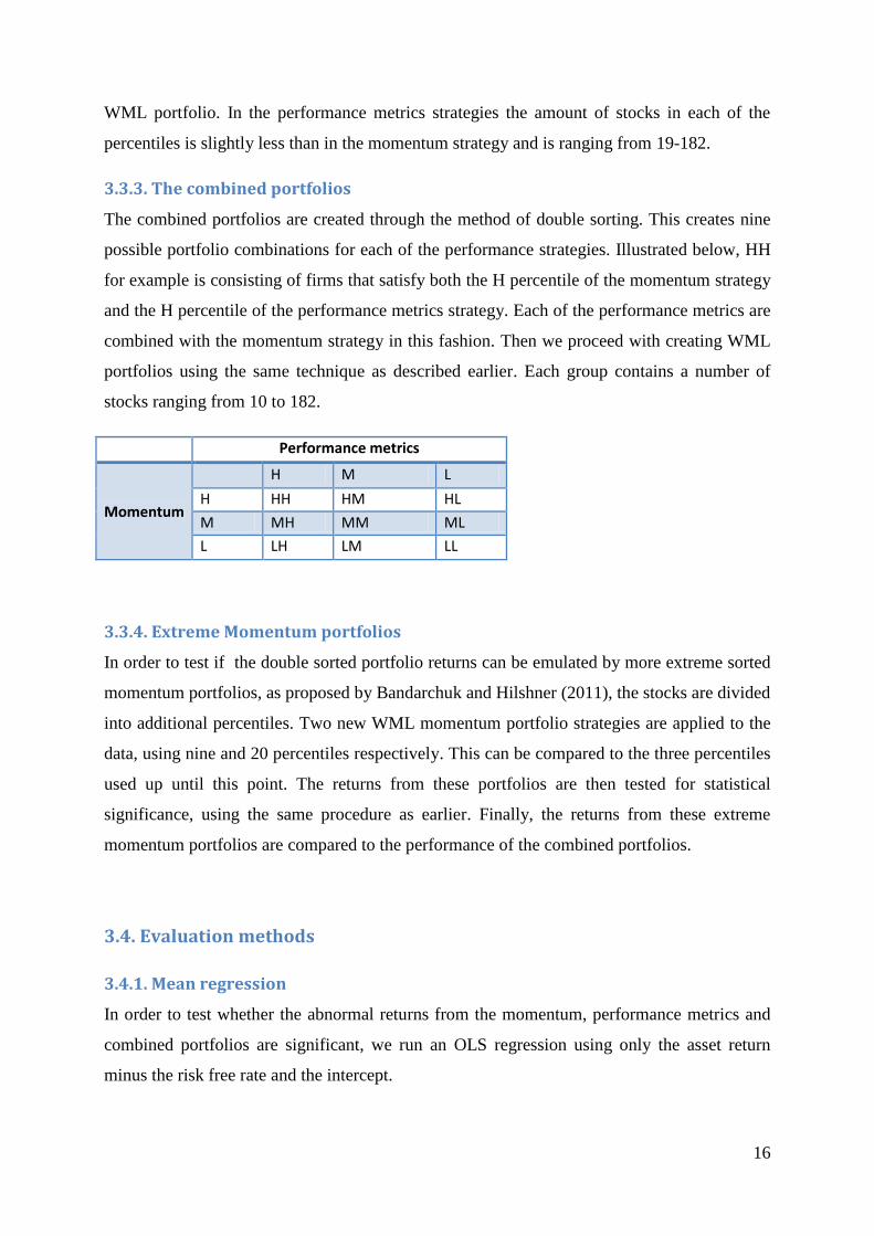
3.3.3. The combined portfolios

The combined portfolios are created through the method of double sorting. This creates nine

possible portfolio combinations for each of the performance strategies. Illustrated below, HH

for example is consisting of firms that satisfy both the H percentile of the momentum strategy

and the H percentile of the performance metrics strategy. Each of the performance metrics are

combined with the momentum strategy in this fashion. Then we proceed with creating WML

portfolios using the same technique as described earlier. Each group contains a number of

stocks ranging from 10 to 182.

Performance metrics

Momentum

H M L

H HH HM HL

M MH MM ML

L LH LM LL

3.3.4. Extreme Momentum portfolios

In order to test if the double sorted portfolio returns can be emulated by more extreme sorted

momentum portfolios, as proposed by Bandarchuk and Hilshner (2011), the stocks are divided

into additional percentiles. Two new WML momentum portfolio strategies are applied to the

data, using nine and 20 percentiles respectively. This can be compared to the three percentiles

used up until this point. The returns from these portfolios are then tested for statistical

significance, using the same procedure as earlier. Finally, the returns from these extreme

momentum portfolios are compared to the performance of the combined portfolios.

3.4. Evaluation methods

3.4.1. Mean regression

In order to test whether the abnormal returns from the momentum, performance metrics and

combined portfolios are significant, we run an OLS regression using only the asset return

minus the risk free rate and the intercept.

17

where is the return of the portfolios and is the intercept which represents the mean

value of the returns. We run this regression on all portfolio combinations that are analyzed

and evaluated in this paper.

3.4.2. Controlling for market risk

To control for market risk we apply the capital asset pricing model, CAPM, developed by

Sharpe (1964), Lintner (1965) and Black (1972), to analyze the theoretical market returns. We

then use Jensen’s alpha to derive the abnormal return above the theoretical market return as

defined by CAPM. By using this theoretical approach on the portfolios, returns originated

from market movements are absorbed by the beta variable, leaving the alpha as the indicator

of abnormal returns. The formula looks as following:

Where = excess return of asset i, = abnormal return of asset i, = excess

return of the market.

3.4.3. Controlling for value and size in addition to market risk

In 1992 Fama and French proposed an alternative approach to measuring return performance

of assets. By adding two additional variables to the commonly used CAPM, it is possible to

account for the value and size characteristics which both have been proven to be relevant

when explaining stock returns. These two variables are created by forming portfolios based on

their book-to-market ratio and size respectively. Stocks with a large (small) book-to-market

ratio are value (growth) stocks. After sorting stocks based on these criteria the loser portfolios’

returns are subtracted from the winner portfolios’ returns. The long short position for size

based stocks is labeled small minus big (SMB) while high minus low (HML) is the acronym

for value sorted portfolios. The formula looks as following:

Where = excess return of asset i, = abnormal return of asset i, = excess

return of the market, = small minus big portfolio and = high minus low portfolio.

18

4. Results/Analysis

In this chapter we present and analyze our results. The portfolio returns mentioned in this

section are all derived on a six month basis.

4.1. Mean regression

4.1.1. Single sorted portfolios

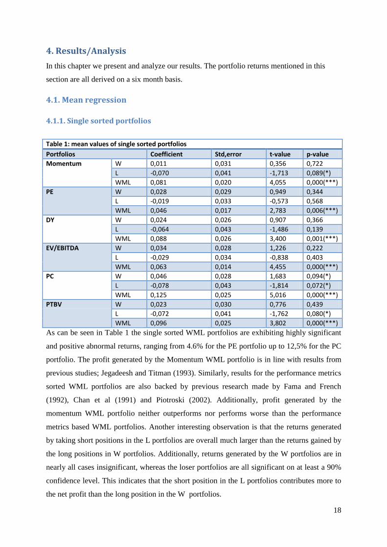
As can be seen in Table 1 the single sorted WML portfolios are exhibiting highly significant

and positive abnormal returns, ranging from 4.6% for the PE portfolio up to 12,5% for the PC

portfolio. The profit generated by the Momentum WML portfolio is in line with results from

previous studies; Jegadeesh and Titman (1993). Similarly, results for the performance metrics

sorted WML portfolios are also backed by previous research made by Fama and French

(1992), Chan et al (1991) and Piotroski (2002). Additionally, profit generated by the

momentum WML portfolio neither outperforms nor performs worse than the performance

metrics based WML portfolios. Another interesting observation is that the returns generated

by taking short positions in the L portfolios are overall much larger than the returns gained by

the long positions in W portfolios. Additionally, returns generated by the W portfolios are in

nearly all cases insignificant, whereas the loser portfolios are all significant on at least a 90%

confidence level. This indicates that the short position in the L portfolios contributes more to

the net profit than the long position in the W portfolios.

Table 1: mean values of single sorted portfolios

Portfolios Coefficient Std,error t-value p-value

Momentum W 0,011 0,031 0,356 0,722

L -0,070 0,041 -1,713 0,089(*)

WML 0,081 0,020 4,055 0,000(***)

PE W 0,028 0,029 0,949 0,344

L -0,019 0,033 -0,573 0,568

WML 0,046 0,017 2,783 0,006(***)

DY W 0,024 0,026 0,907 0,366

L -0,064 0,043 -1,486 0,139

WML 0,088 0,026 3,400 0,001(***)

EV/EBITDA W 0,034 0,028 1,226 0,222

L -0,029 0,034 -0,838 0,403

WML 0,063 0,014 4,455 0,000(***)

PC W 0,046 0,028 1,683 0,094(*)

L -0,078 0,043 -1,814 0,072(*)

WML 0,125 0,025 5,016 0,000(***)

PTBV W 0,023 0,030 0,776 0,439

L -0,072 0,041 -1,762 0,080(*)

WML 0,096 0,025 3,802 0,000(***)

19

4.1.2. Double sorted portfolios

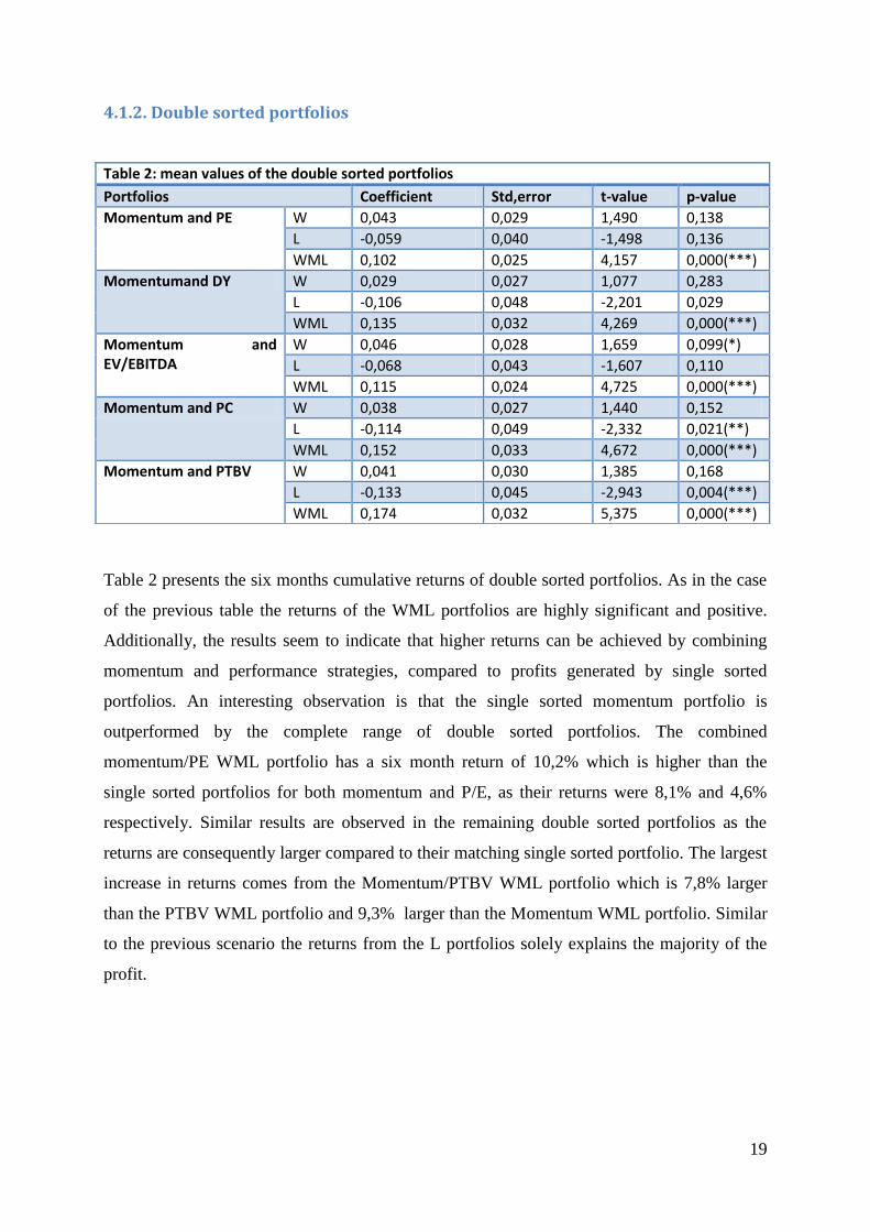
Table 2 presents the six months cumulative returns of double sorted portfolios. As in the case

of the previous table the returns of the WML portfolios are highly significant and positive.

Additionally, the results seem to indicate that higher returns can be achieved by combining

momentum and performance strategies, compared to profits generated by single sorted

portfolios. An interesting observation is that the single sorted momentum portfolio is

outperformed by the complete range of double sorted portfolios. The combined

momentum/PE WML portfolio has a six month return of 10,2% which is higher than the

single sorted portfolios for both momentum and P/E, as their returns were 8,1% and 4,6%

respectively. Similar results are observed in the remaining double sorted portfolios as the

returns are consequently larger compared to their matching single sorted portfolio. The largest

increase in returns comes from the Momentum/PTBV WML portfolio which is 7,8% larger

than the PTBV WML portfolio and 9,3% larger than the Momentum WML portfolio. Similar

to the previous scenario the returns from the L portfolios solely explains the majority of the

profit.

Table 2: mean values of the double sorted portfolios

Portfolios Coefficient Std,error t-value p-value

Momentum and PE W 0,043 0,029 1,490 0,138

L -0,059 0,040 -1,498 0,136

WML 0,102 0,025 4,157 0,000(***)

Momentumand DY W 0,029 0,027 1,077 0,283

L -0,106 0,048 -2,201 0,029

WML 0,135 0,032 4,269 0,000(***)

Momentum and EV/EBITDA

W 0,046 0,028 1,659 0,099(*)

L -0,068 0,043 -1,607 0,110

WML 0,115 0,024 4,725 0,000(***)

Momentum and PC W 0,038 0,027 1,440 0,152

L -0,114 0,049 -2,332 0,021(**)

WML 0,152 0,033 4,672 0,000(***)

Momentum and PTBV W 0,041 0,030 1,385 0,168

L -0,133 0,045 -2,943 0,004(***)

WML 0,174 0,032 5,375 0,000(***)

20

4.2. Controlling for market risk


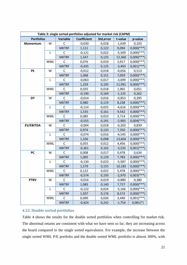
When controlling for market risk results are quite similar to the ones above, illustrated in

Table 3. The WML portfolios are all showing highly significant values on the intercept,

implying that abnormal returns can be achieved with strategies using a single sorting method

based on either momentum or performance metrics. The momentum WML portfolio generates

an abnormal semi annual return of 7.6% while the best performing performance metrics

WML portfolio, PC, has a six month abnormal return of 12,2%. Analyzing the winners and

losers portfolios in Table 3 there is, again, the short positions in the L portfolios that carry the

majority of the profit. The L portfolios are showing large and significant negative returns,

down to as much as minus 13% for the PC losers portfolio.

The observed coefficients for the MKTRF variable indicate that the L portfolios consistently

display a larger exposure toward market movements. Additionally they are all, apart from the

P/E based portfolio, highly significant. Due to the fact that the L portfolios also have higher

market coefficients than their W portfolio counterparts the same coefficient for the WML

portfolios turn slightly negative, around -0,4 on average. Despite coefficients for the market

index being large and significant for the W and L portfolios, the abnormal returns generated

by the WML portfolios are still prevalent but slightly lower across the board compared to the

mean regression analyze of the single sorted portfolios.

21

Table 3: single sorted portfolios adjusted for market risk (CAPM)

Portfolios Variable Coefficient Std,error t-value p-value

Momentum W C -0,030 0,018 -1,639 0,103

MKTRF 1,111 0,122 9,094 0,000(***)

L C -0,121 0,022 -5,509 0,000(***)

MKTRF 1,547 0,125 12,360 0,000(***)

WML C 0,076 0,019 3,917 0,000(***)

MKTRF -0,435 0,125 -3,493 0,001(***)

PE W C -0,012 0,018 -0,656 0,513

MKTRF 1,068 0,151 7,059 0,000(***)

L C -0,063 0,017 -3,699 0,000(***)

MKTRF 1,259 0,105 11,991 0,000(***)

WML C 0,035 0,018 1,965 0,051

MKTRF -0,190 0,169 -1,125 0,262

DY W C -0,014 0,016 -0,853 0,395

MKTRF 0,980 0,119 8,238 0,000(***)

L C -0,114 0,025 -4,616 0,000(***)

MKTRF 1,535 0,161 9,542 0,000(***)

WML C 0,085 0,023 3,714 0,000(***)

MKTRF -0,555 0,191 -2,905 0,004(***)

EV/EBITDA W C -0,004 0,018 -0,203 0,839

MKTRF 0,974 0,133 7,350 0,000(***)

L C -0,074 0,016 -4,545 0,000(***)

MKTRF 1,336 0,098 13,604 0,000(***)

WML C 0,055 0,012 4,456 0,000(***)

MKTRF -0,361 0,102 -3,535 0,001(***)

PC W C 0,008 0,017 0,478 0,634

MKTRF 1,005 0,129 7,783 0,000(***)

L C -0,130 0,023 -5,587 0,000(***)

MKTRF 1,579 0,155 10,185 0,000(***)

WML C 0,122 0,022 5,478 0,000(***)

MKTRF -0,574 0,193 -2,970 0,003(***)

PTBV W C -0,016 0,019 -0,880 0,380

MKTRF 1,083 0,140 7,727 0,000(***)

L C -0,122 0,024 -5,166 0,000(***)

MKTRF 1,507 0,176 8,572 0,000(***)

WML C 0,090 0,026 3,440 0,001(***)

MKTRF -0,424 0,242 -1,754 0,081(*)

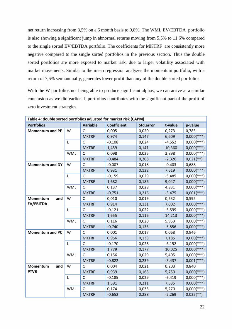
4.22. Double sorted portfolios

Table 4 shows the results for the double sorted portfolios when controlling for market risk.

The abnormal returns are consistent with what we have seen so far, they are increasing across

the board compared to the single sorted equivalence. For example, the increase between the

single sorted WML P/E portfolio and the double sorted WML portfolio is almost 300%, with

22

net return increasing from 3,5% on a 6 month basis to 9,8%. The WML EV/EBTDA portfolio

is also showing a significant jump in abnormal returns moving from 5,5% to 11,6% compared

to the single sorted EV/EBTDA portfolio. The coefficients for MKTRF are consistently more

negative compared to the single sorted portfolios in the previous section. Thus the double

sorted portfolios are more exposed to market risk, due to larger volatility associated with

market movements. Similar to the mean regression analyzes the momentum portfolio, with a

return of 7,6% semiannually, generates lower profit than any of the double sorted portfolios.

With the W portfolios not being able to produce significant alphas, we can arrive at a similar

conclusion as we did earlier. L portfolios contributes with the significant part of the profit of

zero investment strategies.

Table 4: double sorted portfolios adjusted for market risk (CAPM)

Portfolios Variable Coefficient Std,error t-value p-value

Momentum and PE W C 0,005 0,020 0,273 0,785

MKTRF 0,974 0,147 6,609 0,000(***)

L C -0,108 0,024 -4,552 0,000(***)

MKTRF 1,459 0,141 10,360 0,000(***)

WML C 0,098 0,025 3,898 0,000(***)

MKTRF -0,484 0,208 -2,326 0,021(**)

Momentum and DY W C -0,007 0,018 -0,403 0,688

MKTRF 0,931 0,122 7,619 0,000(***)

L C -0,159 0,029 -5,485 0,000(***)

MKTRF 1,682 0,186 9,047 0,000(***)

WML C 0,137 0,028 4,831 0,000(***)

MKTRF -0,751 0,216 -3,475 0,001(***)

Momentum and EV/EBITDA

W C 0,010 0,019 0,532 0,595

MKTRF 0,914 0,131 7,002 0,000(***)

L C -0,121 0,022 -5,599 0,000(***)

MKTRF 1,655 0,116 14,213 0,000(***)

WML C 0,116 0,020 5,953 0,000(***)

MKTRF -0,740 0,133 -5,556 0,000(***)

Momentum and PC W C 0,001 0,017 0,068 0,946

MKTRF 0,956 0,133 7,185 0,000(***)

L C -0,170 0,028 -6,152 0,000(***)

MKTRF 1,779 0,177 10,025 0,000(***)

WML C 0,156 0,029 5,405 0,000(***)

MKTRF -0,822 0,239 -3,437 0,001(***)

Momentum and PTVB

W C 0,004 0,021 0,203 0,840

MKTRF 0,939 0,163 5,750 0,000(***)

L C -0,185 0,029 -6,419 0,000(***)

MKTRF 1,591 0,211 7,535 0,000(***)

WML C 0,174 0,033 5,270 0,000(***)

MKTRF -0,652 0,288 -2,269 0,025(**)

23

4.3. Controlling for market risk, size and value


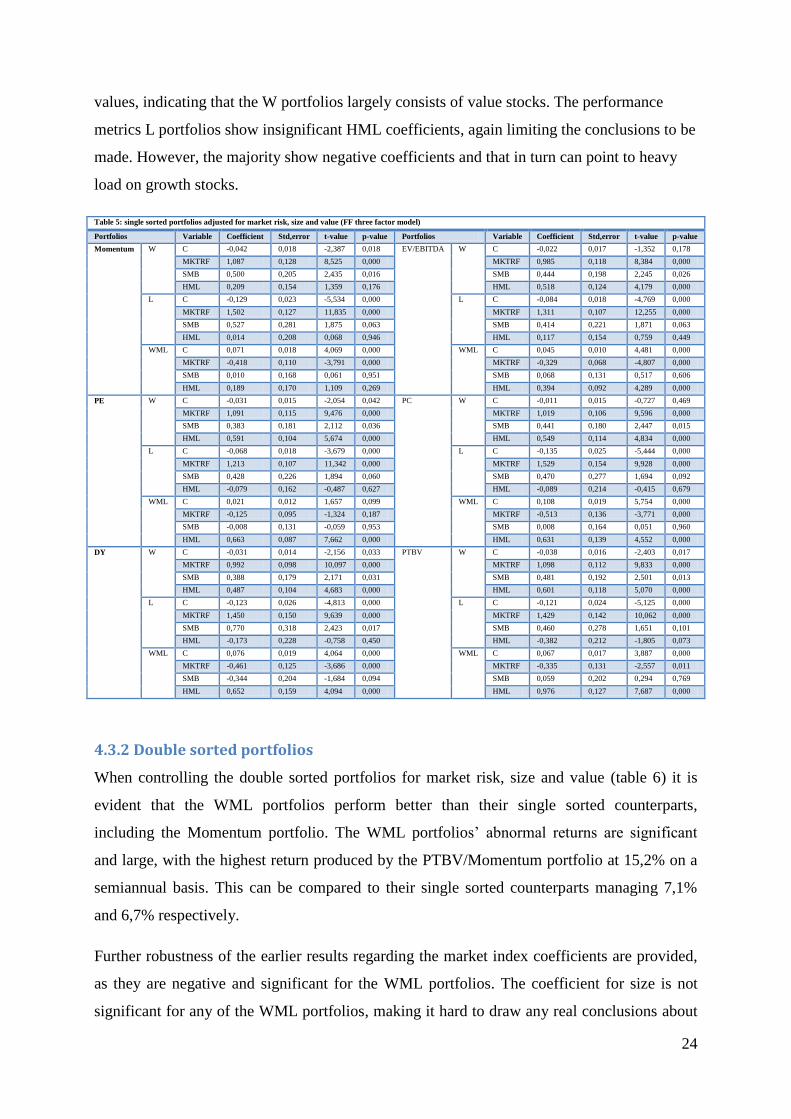
In this part we examine the results from the FF three factor model where returns are

controlled for market risk, size and value. Starting with the abnormal returns for the WML

portfolios, they are highly significant and positive and this is a result consistent with our

previous findings. However, each of these values are notably lower than their equivalence

found in the CAPM regression analyzes. This indicates that size and value play a role when

determining the profits from momentum and performance metrics strategies.

The MKTRF coefficients for the WML portfolios are significant in all cases with negative

values. This is similar to our findings in the CAPM regressions.

When controlling for size using the SMB variable, all but one WML portfolio coefficients are

insignificant, therefore size cannot explain profit generated by the single sorted WML

portfolios. A possible reason for why the D/Y sorted WML portfolios have a significant and

positive loading on the size variable is that, intuitionally, dividends are positively correlated

with the company size.

The entire range of W and L portfolios in table 4 have significant and positive size

coefficients, indicating that there is an overrepresentation of small firms in these portfolios.

This implies that small firms have both the possibility to generate high abnormal returns while

simultaneously carrying the risk of large declines. This is in line with previous research, as

small firms in general have larger volatility than large firms. From the results from table 4 it

also seems like the portfolios with the highest positive loadings to small firms seems to show

the highest volatility in their abnormal returns. This is all supported by studies like Hong, Lim

and Stein (2000) and Zhang (2006), where the former concludes that momentum profits

decline with increasing firm size and the latter proposes that it is volatility that amplifies

momentum profits.

The value variable HML shows significant and positive coefficients for the performance

metrics WML portfolios, implying that they can explain parts of the abnormal returns they are

showing and that they are consisting more heavily of value stocks. The HML beta for the

momentum portfolio is insignificant and hence nothing can be said about whether HML

accounts for parts of the abnormal returns derived from the momentum WML portfolio. All

the HML coefficients for the W performance metrics portfolios show positive and significant

24

values, indicating that the W portfolios largely consists of value stocks. The performance

metrics L portfolios show insignificant HML coefficients, again limiting the conclusions to be

made. However, the majority show negative coefficients and that in turn can point to heavy

load on growth stocks.

Table 5: single sorted portfolios adjusted for market risk, size and value (FF three factor model)

Portfolios Variable Coefficient Std,error t-value p-value Portfolios Variable Coefficient Std,error t-value p-value

Momentum W C -0,042 0,018 -2,387 0,018 EV/EBITDA W C -0,022 0,017 -1,352 0,178

MKTRF 1,087 0,128 8,525 0,000 MKTRF 0,985 0,118 8,384 0,000

SMB 0,500 0,205 2,435 0,016 SMB 0,444 0,198 2,245 0,026

HML 0,209 0,154 1,359 0,176 HML 0,518 0,124 4,179 0,000

L C -0,129 0,023 -5,534 0,000 L C -0,084 0,018 -4,769 0,000

MKTRF 1,502 0,127 11,835 0,000 MKTRF 1,311 0,107 12,255 0,000

SMB 0,527 0,281 1,875 0,063 SMB 0,414 0,221 1,871 0,063

HML 0,014 0,208 0,068 0,946 HML 0,117 0,154 0,759 0,449

WML C 0,071 0,018 4,069 0,000 WML C 0,045 0,010 4,481 0,000

MKTRF -0,418 0,110 -3,791 0,000 MKTRF -0,329 0,068 -4,807 0,000

SMB 0,010 0,168 0,061 0,951 SMB 0,068 0,131 0,517 0,606

HML 0,189 0,170 1,109 0,269 HML 0,394 0,092 4,289 0,000

PE W C -0,031 0,015 -2,054 0,042 PC W C -0,011 0,015 -0,727 0,469

MKTRF 1,091 0,115 9,476 0,000 MKTRF 1,019 0,106 9,596 0,000

SMB 0,383 0,181 2,112 0,036 SMB 0,441 0,180 2,447 0,015

HML 0,591 0,104 5,674 0,000 HML 0,549 0,114 4,834 0,000

L C -0,068 0,018 -3,679 0,000 L C -0,135 0,025 -5,444 0,000

MKTRF 1,213 0,107 11,342 0,000 MKTRF 1,529 0,154 9,928 0,000

SMB 0,428 0,226 1,894 0,060 SMB 0,470 0,277 1,694 0,092

HML -0,079 0,162 -0,487 0,627 HML -0,089 0,214 -0,415 0,679

WML C 0,021 0,012 1,657 0,099 WML C 0,108 0,019 5,754 0,000

MKTRF -0,125 0,095 -1,324 0,187 MKTRF -0,513 0,136 -3,771 0,000

SMB -0,008 0,131 -0,059 0,953 SMB 0,008 0,164 0,051 0,960

HML 0,663 0,087 7,662 0,000 HML 0,631 0,139 4,552 0,000

DY W C -0,031 0,014 -2,156 0,033 PTBV W C -0,038 0,016 -2,403 0,017

MKTRF 0,992 0,098 10,097 0,000 MKTRF 1,098 0,112 9,833 0,000

SMB 0,388 0,179 2,171 0,031 SMB 0,481 0,192 2,501 0,013

HML 0,487 0,104 4,683 0,000 HML 0,601 0,118 5,070 0,000

L C -0,123 0,026 -4,813 0,000 L C -0,121 0,024 -5,125 0,000

MKTRF 1,450 0,150 9,639 0,000 MKTRF 1,429 0,142 10,062 0,000

SMB 0,770 0,318 2,423 0,017 SMB 0,460 0,278 1,651 0,101

HML -0,173 0,228 -0,758 0,450 HML -0,382 0,212 -1,805 0,073

WML C 0,076 0,019 4,064 0,000 WML C 0,067 0,017 3,887 0,000

MKTRF -0,461 0,125 -3,686 0,000 MKTRF -0,335 0,131 -2,557 0,011

SMB -0,344 0,204 -1,684 0,094 SMB 0,059 0,202 0,294 0,769

HML 0,652 0,159 4,094 0,000 HML 0,976 0,127 7,687 0,000

4.3.2 Double sorted portfolios

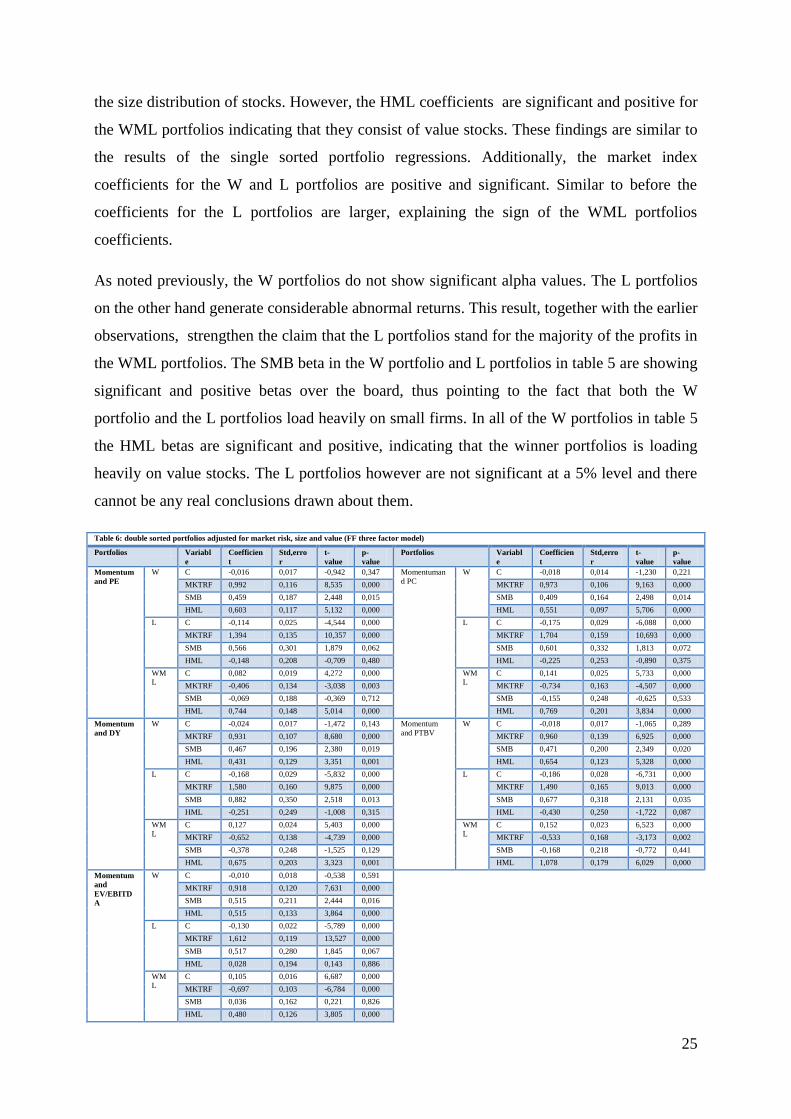
When controlling the double sorted portfolios for market risk, size and value (table 6) it is

evident that the WML portfolios perform better than their single sorted counterparts,

including the Momentum portfolio. The WML portfolios’ abnormal returns are significant

and large, with the highest return produced by the PTBV/Momentum portfolio at 15,2% on a

semiannual basis. This can be compared to their single sorted counterparts managing 7,1%

and 6,7% respectively.

Further robustness of the earlier results regarding the market index coefficients are provided,

as they are negative and significant for the WML portfolios. The coefficient for size is not

significant for any of the WML portfolios, making it hard to draw any real conclusions about

25

the size distribution of stocks. However, the HML coefficients are significant and positive for

the WML portfolios indicating that they consist of value stocks. These findings are similar to

the results of the single sorted portfolio regressions. Additionally, the market index

coefficients for the W and L portfolios are positive and significant. Similar to before the

coefficients for the L portfolios are larger, explaining the sign of the WML portfolios

coefficients.

As noted previously, the W portfolios do not show significant alpha values. The L portfolios

on the other hand generate considerable abnormal returns. This result, together with the earlier

observations, strengthen the claim that the L portfolios stand for the majority of the profits in

the WML portfolios. The SMB beta in the W portfolio and L portfolios in table 5 are showing

significant and positive betas over the board, thus pointing to the fact that both the W

portfolio and the L portfolios load heavily on small firms. In all of the W portfolios in table 5

the HML betas are significant and positive, indicating that the winner portfolios is loading

heavily on value stocks. The L portfolios however are not significant at a 5% level and there

cannot be any real conclusions drawn about them.

Table 6: double sorted portfolios adjusted for market risk, size and value (FF three factor model)

Portfolios Variabl

e

Coefficien

t

Std,erro

r

t-

value

p-

value

Portfolios Variabl

e

Coefficien

t

Std,erro

r

t-

value

p-

value

Momentum

and PE

W C -0,016 0,017 -0,942 0,347 Momentuman

d PC

W C -0,018 0,014 -1,230 0,221

MKTRF 0,992 0,116 8,535 0,000 MKTRF 0,973 0,106 9,163 0,000

SMB 0,459 0,187 2,448 0,015 SMB 0,409 0,164 2,498 0,014

HML 0,603 0,117 5,132 0,000 HML 0,551 0,097 5,706 0,000

L C -0,114 0,025 -4,544 0,000 L C -0,175 0,029 -6,088 0,000

MKTRF 1,394 0,135 10,357 0,000 MKTRF 1,704 0,159 10,693 0,000

SMB 0,566 0,301 1,879 0,062 SMB 0,601 0,332 1,813 0,072

HML -0,148 0,208 -0,709 0,480 HML -0,225 0,253 -0,890 0,375

WM

L

C 0,082 0,019 4,272 0,000 WM

L

C 0,141 0,025 5,733 0,000

MKTRF -0,406 0,134 -3,038 0,003 MKTRF -0,734 0,163 -4,507 0,000

SMB -0,069 0,188 -0,369 0,712 SMB -0,155 0,248 -0,625 0,533

HML 0,744 0,148 5,014 0,000 HML 0,769 0,201 3,834 0,000

Momentum

and DY

W C -0,024 0,017 -1,472 0,143 Momentum

and PTBV

W C -0,018 0,017 -1,065 0,289

MKTRF 0,931 0,107 8,680 0,000 MKTRF 0,960 0,139 6,925 0,000

SMB 0,467 0,196 2,380 0,019 SMB 0,471 0,200 2,349 0,020

HML 0,431 0,129 3,351 0,001 HML 0,654 0,123 5,328 0,000

L C -0,168 0,029 -5,832 0,000 L C -0,186 0,028 -6,731 0,000

MKTRF 1,580 0,160 9,875 0,000 MKTRF 1,490 0,165 9,013 0,000

SMB 0,882 0,350 2,518 0,013 SMB 0,677 0,318 2,131 0,035

HML -0,251 0,249 -1,008 0,315 HML -0,430 0,250 -1,722 0,087

WM

L

C 0,127 0,024 5,403 0,000 WM

L

C 0,152 0,023 6,523 0,000

MKTRF -0,652 0,138 -4,739 0,000 MKTRF -0,533 0,168 -3,173 0,002

SMB -0,378 0,248 -1,525 0,129 SMB -0,168 0,218 -0,772 0,441

HML 0,675 0,203 3,323 0,001 HML 1,078 0,179 6,029 0,000

Momentum

and

EV/EBITD

A

W C -0,010 0,018 -0,538 0,591

MKTRF 0,918 0,120 7,631 0,000

SMB 0,515 0,211 2,444 0,016

HML 0,515 0,133 3,864 0,000

L C -0,130 0,022 -5,789 0,000

MKTRF 1,612 0,119 13,527 0,000

SMB 0,517 0,280 1,845 0,067

HML 0,028 0,194 0,143 0,886

WM

L

C 0,105 0,016 6,687 0,000

MKTRF -0,697 0,103 -6,784 0,000

SMB 0,036 0,162 0,221 0,826

HML 0,480 0,126 3,805 0,000

26

4.4. Extreme momentum portfolios

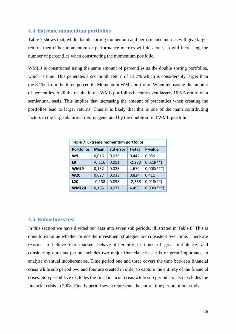
Table 7 shows that, while double sorting momentum and performance metrics will give larger

returns then either momentum or performance metrics will do alone, so will increasing the

number of percentiles when constructing the momentum portfolio.

WML9 is constructed using the same amount of percentiles as the double sorting portfolios,

which is nine. This generates a six month return of 13.2% which is considerably larger than

the 8.1% from the three percentile Momentum WML portfolio. When increasing the amount

of percentiles to 20 the results in the WML portfolios become even larger, 16.5% return on a

semiannual basis. This implies that increasing the amount of percentiles when creating the

portfolios lead to larger returns. Thus it is likely that this is one of the main contributing

factors to the large abnormal returns generated by the double sorted WML portfolios.

Table 7: Extreme momentum portfolios

Portfolios Mean std error T-stat P-value

W9 0,016 0,035 0,442 0,659

L9 -0,116 0,051 -2,290 0,023(**)

WML9 0,132 0,028 4,679 0,000(***)

W20 0,027 0,033 0,824 0,411

L20 -0,138 0,058 -2,388 0,018(**)

WML20 0,165 0,037 4,493 0,000(***)

4.5. Robustness test

In this section we have divided our data into seven sub periods, illustrated in Table 8. This is

done to examine whether or not the investment strategies are consistent over time. There are

reasons to believe that markets behave differently in times of great turbulence, and

considering our data period includes two major financial crisis it is of great importance to

analyze eventual incoherencies. Time period one and three covers the time between financial

crisis while sub period two and four are created in order to capture the entirety of the financial

crises. Sub period five excludes the first financial crisis while sub period six also excludes the

financial crisis in 2008. Finally period seven represents the entire time period of our study.

27

Table 8: Time periods

1 1996m12-1999m12

2 2000m01-2002m12

3 2003m01-2008m08

4 2008m09 2010m12

5 1996m12-1999m12, 2003m01-2010m12

6 1996m12-1999m12, 2003m01-2008m08

7 1996m12-2010m12

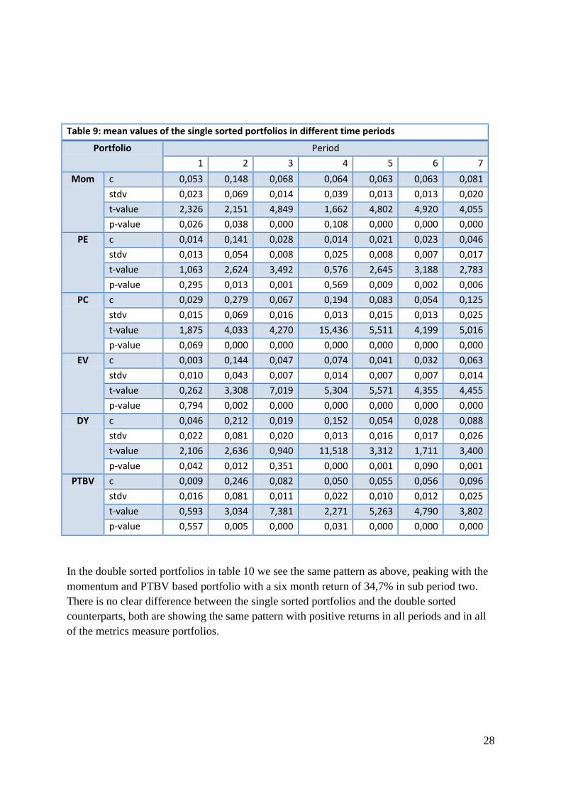
Table 8 provides the results for the single sorted portfolios. The table reveals that the largest

returns from all portfolios can be found in sub period two. During the first financial crisis, the

returns for both the momentum based portfolios and the value based portfolios are two to

three times larger than the returns throughout the entire period. In sub period four, illustrating

the second financial crisis, only the D/Y and EV/EBITDA sorted portfolios achieve similar

returns. The loser portfolios display significant negative returns during the financial crisis.

This adds to the intuition, given the above results, that the short positions in the loser

portfolios constitutes the lion’s share of the large abnormal returns.

The general conclusion , from the table below, is that the WML portfolios generate positive

abnormal returns throughout all the sub periods.

28

Table 9: mean values of the single sorted portfolios in different time periods

Portfolio Period

1 2 3 4 5 6 7

Mom c 0,053 0,148 0,068 0,064 0,063 0,063 0,081

stdv 0,023 0,069 0,014 0,039 0,013 0,013 0,020

t-value 2,326 2,151 4,849 1,662 4,802 4,920 4,055

p-value 0,026 0,038 0,000 0,108 0,000 0,000 0,000

PE c 0,014 0,141 0,028 0,014 0,021 0,023 0,046

stdv 0,013 0,054 0,008 0,025 0,008 0,007 0,017

t-value 1,063 2,624 3,492 0,576 2,645 3,188 2,783

p-value 0,295 0,013 0,001 0,569 0,009 0,002 0,006

PC c 0,029 0,279 0,067 0,194 0,083 0,054 0,125

stdv 0,015 0,069 0,016 0,013 0,015 0,013 0,025

t-value 1,875 4,033 4,270 15,436 5,511 4,199 5,016

p-value 0,069 0,000 0,000 0,000 0,000 0,000 0,000

EV c 0,003 0,144 0,047 0,074 0,041 0,032 0,063

stdv 0,010 0,043 0,007 0,014 0,007 0,007 0,014

t-value 0,262 3,308 7,019 5,304 5,571 4,355 4,455

p-value 0,794 0,002 0,000 0,000 0,000 0,000 0,000

DY c 0,046 0,212 0,019 0,152 0,054 0,028 0,088

stdv 0,022 0,081 0,020 0,013 0,016 0,017 0,026

t-value 2,106 2,636 0,940 11,518 3,312 1,711 3,400

p-value 0,042 0,012 0,351 0,000 0,001 0,090 0,001

PTBV c 0,009 0,246 0,082 0,050 0,055 0,056 0,096

stdv 0,016 0,081 0,011 0,022 0,010 0,012 0,025

t-value 0,593 3,034 7,381 2,271 5,263 4,790 3,802

p-value 0,557 0,005 0,000 0,031 0,000 0,000 0,000

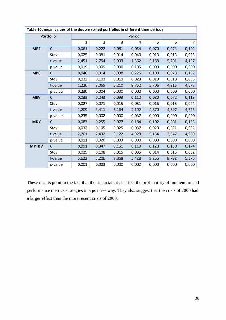
In the double sorted portfolios in table 10 we see the same pattern as above, peaking with the

momentum and PTBV based portfolio with a six month return of 34,7% in sub period two.

There is no clear difference between the single sorted portfolios and the double sorted

counterparts, both are showing the same pattern with positive returns in all periods and in all

of the metrics measure portfolios.

29

Table 10: mean values of the double sorted portfolios in different time periods

Portfolio Period

1 2 3 4 5 6 7

MPE C 0,061 0,222 0,081 0,054 0,070 0,074 0,102

Stdv 0,025 0,081 0,014 0,040 0,013 0,013 0,025

t-value 2,451 2,754 5,903 1,362 5,188 5,701 4,157

p-value 0,019 0,009 0,000 0,185 0,000 0,000 0,000

MPC C 0,040 0,314 0,098 0,225 0,109 0,078 0,152

Stdv 0,032 0,103 0,019 0,023 0,019 0,018 0,033

t-value 1,220 3,065 5,210 9,752 5,706 4,215 4,672

p-value 0,230 0,004 0,000 0,000 0,000 0,000 0,000

MEV C 0,033 0,243 0,093 0,112 0,080 0,072 0,115

Stdv 0,027 0,071 0,015 0,051 0,016 0,015 0,024

t-value 1,209 3,411 6,164 2,192 4,870 4,697 4,725

p-value 0,235 0,002 0,000 0,037 0,000 0,000 0,000

MDY C 0,087 0,255 0,077 0,184 0,102 0,081 0,135

Stdv 0,032 0,105 0,025 0,037 0,020 0,021 0,032

t-value 2,701 2,432 3,122 4,928 5,154 3,847 4,269

p-value 0,011 0,020 0,003 0,000 0,000 0,000 0,000

MPTBV C 0,091 0,347 0,151 0,119 0,128 0,130 0,174

Stdv 0,025 0,108 0,015 0,035 0,014 0,015 0,032

t-value 3,622 3,206 9,868 3,428 9,255 8,792 5,375

p-value 0,001 0,003 0,000 0,002 0,000 0,000 0,000

These results point to the fact that the financial crisis affect the profitability of momentum and

performance metrics strategies in a positive way. They also suggest that the crisis of 2000 had

a larger effect than the more recent crisis of 2008.

30

5. Conclusion

The final chapter of this essay contains a brief summary and some concluding remarks around

our empirical results. This essay has evaluated the efficiency of the Nordic stock markets by

using investment strategies based on selected market variables. The individual stocks are

ranked according to their past six month relative performance, and sorted by the use of

overlapping six month periods. Based on the stocks relative ranking, they have then been

placed in three different portfolios for each of the selected variables. The worst performing

portfolio has been subtracted from the best performing portfolio, creating the winner minus

loser portfolio (WML) investment strategy. Using these constructed portfolios, this study

examines the possibility of reaching elevated levels of profitability by using both single sorted

portfolios and double sorted portfolios based on the momentum effect and one additional

performance metrics. Finally the performance of the portfolios are compared to a single

sorted momentum strategy which employs a more extreme sorting process, using more and

smaller percentile groups in the evaluation of the stocks.

From section 4.1, using the mean regression analysis, we can see that the entire range of

evaluated single sorted WML portfolios generate abnormal returns. The return based

momentum portfolios, compared to all portfolios, is in the medium range with regards to

profitability. It has a semiannual return of 8,1 percent which can be compared to the value

based portfolios P/C that attained the highest abnormal return, 12,5 percent. The P/E portfolio

proved to be the least profitable with a return of 4,6 percent. So we cannot say that the classic

momentum strategy in general is outperformed by all of the other measures used in the study,

but the mean regression analysis indicates that strategies based on the performance metrics

D/Y,P/C and PTBV arguably perform better than the strategies based on stock returns.

The mean regression analysis of the double sorted portfolios also came out all positive and

significant. They all beat their counterparts in the single sorted portfolios, and even more

interesting, all of them also showed higher returns compared to the momentum strategy. Thus

the mean regression analysis indicates that by using any one of the five measures presented in

the paper, combined with stock returns for the basis of the creation of the WML portfolios,

higher profitability can be achieved compared to the single sorted momentum strategy based

solely on stock returns.

After controlling for market risk by using the CAPM model, the abnormal returns observed

earlier are persistent, while the abnormal returns were in general lower compared to the

31

results from the mean regression analysis, they were still present and rather large. This

indicates that even if market risk can explain parts of the abnormal returns, it is not capable of

fully encapsulating stock returns based on these strategies.

In the Fama and French three factor model analysis the abnormal returns persist, albeit on a

smaller scale compared to the results from the CAPM analysis. This indicates that size and

value can partly explain the large abnormal profits. But considering the abnormal profits are

still significant it is not fully capable of explaining this profitability. Further, it seems like the

winner and loser portfolios load heavy on size, which point to the fact that the profits is

somewhat correlated to the size of the firms. However the size coefficients for the WML

portfolios are insignificant so it is hard to say anything definite. It also seems like the

portfolios with the largest concentration of small firms are also the ones with the highest

volatility, indicating that volatility affects the final return. It seems that value firms can

explain a small part of the return of the performance metrics strategies, which does not come

as a surprise considering these strategies are created based on value based variables.

We also arrived at the conclusion that it is the short position in the loser portfolio that has the

largest contribution to the abnormal returns based on our portfolio strategies. Our numbers

showed large negative and significant returns on the loser portfolios. This conclusion is also

strengthened by the fact that periods of financial crisis increase the profits from momentum

and performance metric strategies.

The fact that the double sorted portfolios seem to outperform their counter parts in the single

sorted strategies, it is not necessarily due to being a dominant investment strategy. A possible

explanation is that there are less firms in the double sorted portfolios and these firms are more

extreme within the various characteristics presented in this paper. Our extreme momentum

test display that larger profits can be achieved solely by elevating the ranking process.

As neither market-risk, size nor value are able to explain the difference in returns between

performance metrics or the large abnormal returns achieved, it is highly probable that the

answers are found in the field of behavioral finance. Our conclusion is that the efficient

market hypothesis does not hold, and that the large abnormal returns can possibly be

explained by the actions of irrational agents, where attributes such as overconfidence and

self-attribution combined with ambiguous interpretation of news and information is causing

investors to react differently. Experimental evidence has been found in the study by Daniel,

K., D. et.al (1998), where over and under reaction of both private and public information is

32

the underlying reason for the profitability of momentum and value based investment strategies.

However, the possibility that investors in fact are rational cannot be ruled out. Crombez (1998)

proposes that the source for these market anomalies can be explained by noise in expert

information. Either way, our study indicates that conventional economic theory fails to

explain the large abnormal returns derived from persistent stock price continuations and value

based investment strategies.

33

6. References

Alicke Mark D., Vredenburg Debbie S., Hiatt Matthew, and Govorun Olesya,

(2001). ”The ”Better Than Myself Effect.” Motivation and Emotion, 25(1).

Asness, C., Moskowitz, T, J., and Pedersen, L, J. (2009). “Value and Momentum Everywhere.”

working paper, National Bureau of Economic Research.

Barberis, N., Shleifer, A., and R. Vishny. (1998). “A Model of Investor Sentiment.” Journal

of Financial Economics, 49.

Bem, D.J. (1965). “An experimental analysis of self-persuasion.” Journal of Experimental

Social Psychology, 1(3), 199–218.

Chan, L, K. C., Hamao, Y.,and Lakonishok, J. (1991). “Fundamentals and stock returns in

Japan.” Journal of Finance 46, 1739–1764.

Chan, L., Jegadeesh, N., and Lakonishok, J. (1996) “Momentum Strategies.” Journal of

Finance 51, 1681-1713.

Cowles III, A., and Jones, H, E. (1937). “Some A Posteriori Probabilities in Stock Market

Action.” Econometrica 5(3), 280-294.

Crombez, J. (2001). “Momentum, Rational Agents and Efficient Markets.” Journal of

Psychology and Financial Markets, 2(4), 190-200.

Daniel, K., Hirschleifer, D., and A. Subrahmanyam. (1998). “A Theory of Overconfidence,

Self-Attribution, and Security Market Under and Over-reactions.” Journal of Finance, 53.

DeBondt, W., and Thaler, R., (1985) “Does the Stock Market Overreact?” The Journal of

Finance, 40, 793-805.

Erb, C., and Harvey, C. (2006). “The Strategic and Tactical Value of Commodity Futures.”

Financial Analysts Journal, 62(2), 69-97.

Evidence and Implications.” Journal of Financial Economics, 22, 27–59.

Fama, E. F., and K.R. French (1992). “The Cross Section of Expected Stock Returns.”

Journal of Finance 47, 427-465.

34

Fama, E. F., and K.R. French (1998) “Value versus growth: the international evidence.”

Journal of Finance 53, 1975-1979.

Hon, Mark T., and Tonks, I. (2003). "Momentum in the UK stock market." Journal of

Multinational Financial Management Elsevier, 13(1), 43-70.

Hong, H., Lim, T., and Stein, J. (2000). “Bad News Travels Slowly: Size, Analyst Coverage,

and the Profitability of Momentum Strategies.” Journal of Finance, 55, 265-295.

Jegadeesh, N., and Titman, S. (1993). “Returns to Buying Winners and Selling Losers:

Implications for Stock Market Efficiency.”Journal of Finance 48(1), 65-91.

Lee, C, M, C., and Swaminathan, B. (2000). "Price Momentum and Trading Volume."

Journal of Finance American Finance Association, 55(5), 2017-2069.

Levy, Robert A. (1967). “Relative Strength as a Criterion for Investment Selection.” Journal

of Finance 22(4), 595-610.

Miffre, J., and Rallis, G. (2007). “Momentum Strategies in Commodity Futures Markets.”

Journal of Banking and Finance, 31 ( 6).

Odean, T. (1998). "Are Investors Reluctant to Realize Their Losses?" Journal of Finance,

53(5), 1775-1798.

Piotroski, J, D. (2002), “Value Investing: The Use of Historical Financial Statement

Information to Separate Winners from Losers.” The University of Chicago School of Business

Poterba, J., and Summers, L. (1988). “Mean Reversion in Stock Prices:

Ronald J. Balvers, R, J., Wu, Y. (2002). "Stock Market Integration, Return Forecastability and

Implications for Market Efficiency: A Panel Study." Working Paper 112002, Hong Kong

Institute for Monetary Research.

Rouwenhorst, K.G. “International Momentum Strategies.” (1998). Journal of Finance, 53,

267-284.

Svenson, O. (1981) "Are we all less risky and more skillful than our fellow drivers?". Acta

Psychologica 47 (2), 143–148.

35

Zhang, X. F, (2006). “Information uncertainty and stock returns,” Journal of Finance 61,

105–137.

36

Appendix 1: Stationarity

In order to test our data for Stationarity we employ the Phillips-Perron test, which tests for a

unit root in the data. All the regressions has P-values that show significance at a 10% level

and all except one shows significance at a 5% level. This means that the null of a unit root in

the data is rejected and we conclude that the data is stationary.

Phillips-Perron test for stationarity

T-statistic P-value T-statistic P-value

Momentum W -3.601945 0.0067 MPE W -3.354546 0.0140

L -3.424896 0.0114 L -3.556793 0.0077

WML -3.962314 0.0021 W-L -3.737395 0.0043

PE W -3.403272 0.0122 MPC W -3.415064 0.0118

L -3.446125 0.0107 L -3.362726 0.0137

WML -3.367052 0.0135 W-L -3.208815 0.0212

DY W -3.470577 0.0100 MDY W -3.520619 0.0086

L -3.446958 0.0107 L -3.462822 0.0102

WML -3.192927 0.0221 W-L -3.435793 0.0111

EV/EBITDA W -3.498692 0.0092 MEV W -3.423104 0.0115

L -3.428213 0.0113 L -3.570109 0.0074

WML -3.388749 0.0127 W-L -4.009017 0.0018

PC W -3.436370 0.0110 MPTBV W -3.338866 0.0147

L -3.272120 0.0178 L -3.427512 0.0113

WML -2.825090 0.0569 W-L -3.388821 0.0127

PTBV W -3.369469 0.0134 HML -3.753731 0.0041

L -3.379105 0.0131 SMB -4.644009 0.0002

WML -3.186843 0.0225 MKRF -3.905930 0.0025

37

2: OLS assumptions

In order to use OLS for statistical testing we need to make sure that:

1. The expected value of the error terms are always zero. This is fulfilled as we have a

constant included in all the equations we are using in the regressions.

2. That the errors are normally distributed. To test for normality, the Jarque-Bera test is used.

If the P-values in the Jarque-Berra test is smaller than 0,05, it means that the null of normality

at a 5% level is rejected. We can however still use this data in our analysis and get unbiased

results due to the large data samples we employ.

Jarque-bera normality test

Constant CAPM FF

Jarque-bera P-value Jarque-bera P-value Jarque-bera P-value

Momentum W 23.25 0 5.28 0.7 1,96 0,38

L 11.33 0 10.89 0 6,97 0,03

W-L 24.65 0 27,83 0 49,46 0

PE W 147,06 0 45,42 0 27,51 0

L 13,86 0 1,58 0,45 0,37 0,83

W-L 38,79 0 14,08 0 5,2 0,07

DY W 83,64 0 51,38 0 20,1 0

L 2,71 0,26 1,86 0,4 0,03 0,98

W-L 13,83 0 10,49 0 2,31 0,32

EV/EBITDA W 74,3 0 49,71 0 11,39 0

L 22,94 0 9,15 0,01 1,74 0,42

W-L 40,69 0 13,01 0 1,37 0,5

PC W 73,26 0 48,41 0 12 0

L 10,31 0,01 2,15 0,34 1,73 0,42

W-L 18,6 0 4,9 0,09 8,92 0,01

PTBV W 63,03 0 31,05 0 8,72 0,01

L 8,47 0,01 0,29 0,86 0,8 0,67

W-L 61,52 0 10,2 0,01 0,64 0,73

MPE W 65,87 0 12,61 0 4,96 0,08

L 13,97 0 13,6 0 14,59 0

W-L 57,69 0 17,11 0 23,36 0

MPC W 97,87 0 22,72 0 9,6 0,01

L 8,03 0,02 0,89 0,64 2,2 0,33

W-L 16,17 0 0,96 0,62 3,04 0,22

MDY W 36,6 0 16,26 0 8,31 0,02

L 2,86 0,24 0,33 0,84 0,7 0,7

W-L 6,9 0,032 4,23 0,12 3,57 0,17

MEV W 29,85 0 16,98 0 2,44 0,3

L 21,22 0 17,56 0 15,68 0

W-L 31,79 0 18,21 0 16,68 0

MPTBV W 42,83 0 4,09 0,13 4,34 0,11

L 7,89 0,02 1,74 0,41 4,78 0,09

W-L 41,55 0 5,09 0,08 1,96 0,38

38

3. The variance of the error terms should be constant, that is an assumption of

homoscedasticity. To test for this we use White´s test, one advantage with this test is that it do

not require normality in the error terms.

White´s test for homoscedasticity

CAPM FF

Obs*R-squared Prob. Chi-Square(2) Obs*R-squared Prob. Chi-Square(2)

Momentum W 9.564454 0.0084 29.86734 0.0005

L 2.702320 0.2589 25.87159 0.0021

WML 10.85005 0.0044 17.33116 0.0438

PE W 5.807327 0.0548 41.06725 0.0000

L 8.919031 0.0116 30.42099 0.0004

WML 30.28153 0.0000 22.28182 0.0080

DY W 1.754526 0.4159 38.11954 0.0000

L 15.27945 0.0005 29.58222 0.0005

WML 10.17549 0.0062 10.50073 0.3115

EV/EBITDA W 2.042814 0.3601 44.10119 0.0000

L 9.912847 0.0070 31.79219 0.0002

WML 7.329331 0.0256 43.44720 0.0000

PC W 2.139842 0.3430 42.63383 0.0000

L 19.85871 0.0000 32.44860 0.0002

WML 21.50421 0.0000 14.34115 0.1107

PTBV W 4.350319 0.1136 38.67346 0.0000

L 9.084159 0.0107 22.21455 0.0082

WML 31.06216 0.0000 29.25290 0.0006

MPE W 2.852203 0.2402 22.38219 0.0077

L 0.132511 0.9359 21.12357 0.0121

W-L 21.43556 0.0000 11.92570 0.2175

MPC W 3.365906 0.1858 38.55022 0.0000

L 7.980646 0.0185 24.84292 0.0031

W-L 11.98469 0.0025 11.97293 0.2148

MDY W 0.796189 0.6716 21.12061 0.0121

L 7.817862 0.0201 21.70411 0.0099

W-L 4.778290 0.0917 7.315357 0.6043

MEV W 3.590483 0.1661 34.16853 0.0001

L 1.065248 0.5871 18.79733 0.0270

W-L 6.024148 0.0492 8.556468 0.4792

MPTBV W 7.967236 0.0186 38.81175 0.0000

L 4.436411 0.1088 21.65515 0.0100

W-L 30.43931 0.0000 20.43704 0.0154

39

4. That there is no presence of autocorrelation. That is that the error terms are uncorrelated

over time. To test for this we use the Durbin-Watson test, which test for first order

autocorrelation. The lower and upper bounds are for CAPM 1,664-1,684 and for FF 1,643-

1,704. If the DW statistical value is less than the lower bound there is a problem with

autocorrelation.

Durbin-Watson, test for first order autocorrelation

CAPM FF

Momentum W 0.315497 0.388558

L 0.339023 0.368829

WML 0.341567 0.347731

PE W 0.241965 0.410312

L 0.316604 0.344792

WML 0.185464 0.259402

DY W 0.247904 0.401526

L 0.280007 0.344155

WML 0.201003 0.254769

EV/EBITDA W 0.224706 0.367443

L 0.346102 0.387225

WML 0.254143 0.311146

PC W 0.228612 0.386581

L 0.309234 0.327903

WML 0.212293 0.234872

PTBV

W 0.230035 0.410886

L 0.295186 0.323187

WML 0.167313 0.266971

MPE

W 0.281035 0.429689

L 0.352112 0.371128

W-L 0.338503 0.409488

MPC

W 0.262837 0.447728

L 0.360292 0.379290

W-L 0.302991 0.324362

MDY

W 0.252814 0.371686

L 0.319163 0.382092

W-L 0.310677 0.354042

MEV

W 0.239473 0.370723

L 0.441395 0.465858

W-L 0.481881 0.539019

MPTBV

W 0.215483 0.366804

L 0.318078 0.342847

W-L 0.261119 0.387878

5. That the data is non-stochastic, this however is not a problem in our analysis since the

regression estimators are consistent and unbiased even in the presence of stochastic regressors.

To correct the effects of hetroskedasticity and autocorrelation in the error terms we use the

Newey-West estimator to get HAC consistent covariances for all our regressions.

Documents

ALPHA ANALYSIS METRICS STUDY OF THE EFFICIENT MARKET