Modelling Valve Stiction 1 - University of Alberta

Accepted for Publication in Control Engineering Practice, 2004

Modelling Valve Stiction 1

M. A. A. Shoukat Choudhury a

N. F. Thornhill b and S.L. Shah a,2

aDepartment of Chemical and Materials Engineering,University of Alberta, Edmonton, Canada, AB T6G 2G6

bDepartment of Electronic and Electrical EngineeringUniversity College London, London, UK WC1E 7JE

Abstract

The presence of nonlinearities, e.g., stiction, and deadband in a control valve limitsthe control loop performance. Stiction is the most commonly found valve problem inthe process industry. In spite of many attempts to understand and model the stictionphenomena, there is a lack of a proper model, which can be understood and relateddirectly to the practical situation as observed in real valves in the process industry.This study focuses on the understanding, from real life data, of the mechanismthat causes stiction and proposes a new data-driven model of stiction, which can bedirectly related to real valves. It also validates the simulation results generated usingthe proposed model with that from a physical model of the valve. Finally, valuableinsights on stiction have been obtained from the describing function analysis of thenewly proposed stiction model.

Key words: stiction, stickband, deadband, hysteresis, backlash, deadzone, viscousfriction, Coulomb friction, process control, slip jump

1 A preliminary version of this paper was presented at ADCHEM 2003, Hong Kong, Jan. 11-14, 20042 Author to whom all correspondence should be addressed, Email: [email protected]; Fax: +1-780-492-2881

Preprint submitted to Elsevier Preprint

1 Introduction

A typical chemical plant has hundreds or thousands of control loops. Controlperformance is very important to ensure tight product quality and low cost ofthe product in such plants. The economic benefits resulting from performanceassessment are difficult to quantify on a loop-by-loop basis because each prob-lem loop contributes in a complicated way to the overall process performance.Finding and fixing problem loops throughout a plant shows reduced off-gradeproduction, reduced product property variability, and occasionally lower op-erating costs and improved production rate (Paulonis and Cox, 2003). Even a1% improvement either in energy efficiency or improved controller maintenancedirection represents hundreds of millions of dollars in savings to the processindustries (Desborough and Miller, 2002). Oscillatory variables are one of themain causes for poor performance of control loops and a key challenge is to findthe root cause of distributed oscillations in chemical plants (Qin, 1998; Thorn-hill et al., 2003a; Thornhill et al., 2003b). The presence of oscillations in a con-trol loop increases the variability of the process variables thus causing inferiorquality products, larger rejection rates, increased energy consumption, reducedaverage throughput and profitability. Oscillations can cause a valve to wear outmuch earlier than its life period it was originally designed for. Oscillations in-creases operating costs roughly in proportion to the deviation (Shinskey, 1990).Detection and diagnosis of the causes of oscillations in process operation areimportant because a plant operating close to product quality limit is moreprofitable than a plant that has to back away because of variations in theproduct (Martin et al., 1991). Oscillatory feedback control loops are a commonoccurrence due to poor controller tuning, control valve stiction, poor processand control system design, and oscillatory disturbances (Bialkowski, 1992; En-der, 1993; Miao and Seborg, 1999). Bialkowski (1992) reported that about 30%of the loops are oscillatory due to control valve problems. The only movingpart in a control loop is the control valve. If the control valve contains non-linearities, e.g., stiction, backlash, and deadband, the valve output may beoscillatory which in turn can cause oscillations in the process output. Amongthe many types of nonlinearities in control valves, stiction is the most commonand one of the long-standing problems in the process industry. It hinders theachievement of good performance of control valves as well as control loops.Many studies (Armstrong-Helouvry et al., 1994; Aubrun et al., 1995; McMil-lan, 1995; Taha et al., 1996; Wallen, 1997; Horch and Isaksson, 1998; Sharifand Grosvenor, 1998; Horch et al., 2000; Horch, 2000; Ruel, 2000; Gerry andRuel, 2001) have been carried out to define and detect static friction or stiction.However, there is lack of a unique definition and description of the mechanismof stiction. This work addresses this issue and modelling of valve friction. Theparameters of a physical model, e.g., mass of the moving parts of the valve,spring constants, and forces, are not explicitly known. These parameters needto be tuned properly to produce the desired response of a valve. The effect of

2

changes in these parameters are also not known. Working with such a phys-ical model is therefore often time consuming and cumbersome for simulationpurposes. Also, in industrial practice stiction and other related problems areidentified in terms of the % of the valve travel or span of the valve input sig-nal. The relationship between the magnitudes of the parameters of a physicalmodel and deadband, backlash or stiction (expressed as a % of the span of theinput signal) is not simple. The purpose of this paper is to develop an empir-ical data-driven model of stiction that is useful for simulation and diagnosisof oscillation in chemical processes. The main contributions of this paper are:

• Clarification of the confusion prevailed in the control literature and in thecontrol community regarding the misunderstanding of stiction and the termsclosely related to it.

• A new formal definition of stiction has been proposed using parameters sim-ilar to those used in the American National Standard Institution’s (ANSI)formal definition of backlash, hysteresis, and deadband. The key feature ofthese definitions is that they focus on the input-output behaviour of suchelements. The proposed definition is also cast in terms of the input-outputbehaviour.

• A new two parameter data driven model of stiction has been developed andvalidated with a mechanistic model of stiction and also with data obtainedfrom industrial control valves suffering from stiction. The data driven modelis capable of handling stochastic inputs and can be be used to performsimulation of stiction in Matlab’s Simulink environment in the studies ofstiction relevant control loop problems.

• A describing function analysis of the newly proposed stiction model revealsvaluable insights on stiction behaviour. For example, pure deadband or back-lash can not produce limit cycles in the presence of a PI controller unlessthere is an integrator in the plant under closed loop feedback configuration.

The paper has been organized as follows: First, a thorough discussion of theterms related to valve nonlinearity has been presented, followed by the pro-posal of a new formal definition of stiction. Some practical examples of valvestiction are provided to gain true insights of stiction from real life data. Thenthe results of a mechanistic model of stiction was used to validate the cor-responding subsequent results of the data driven stiction model. Finally, adescribing function analysis of the newly proposed stiction model has beenpresented.

2 What is Stiction?

There are some terms such as deadband, backlash and hysteresis which areoften misused and wrongly used in describing valve problems. For example,

3

quite commonly a deadband in a valve is referred to backlash or hysteresis.Therefore, before proceeding to the definition of stiction, these terms are firstdefined for a better understanding of the stiction mechanism and a more formaldefinition of stiction.

2.1 Definition of terms relating to valve nonlinearity

This section reviews the American National Standard Institution’s (ANSI)formal definition of terms related to stiction. The aim is to differentiate clearlybetween the key concepts that underlie the ensuing discussion of friction incontrol valves. These definition can also be found in (EnTech, 1998; Fisher-Rosemount, 1999), which also make reference to ANSI. ANSI (ISA-S51.1-1979,Process instrumentation Terminology) defines the above terms as follows:

• Backlash: “In process instrumentation, it is a relative movement betweeninteracting mechanical parts, resulting from looseness, when the motion isreversed”.

• Hysteresis: “Hysteresis is that property of the element evidenced by the de-pendence of the value of the output, for a given excursion of the input, uponthe history of prior excursions and the direction of the current traverse”.· “It is usually determined by subtracting the value of deadband from the

maximum measured separation between upscale going and downscale goingindications of the measured variable (during a full range traverse, unlessotherwise specified) after transients have decayed”. Figure 1(a) and (c)illustrates the concept.

· “Some reversal of output may be expected for any small reversal of input.This distinguishes hysteresis from deadband”.

• Dead band: “In process instrumentation, it is the range through which aninput signal may be varied, upon reversal of direction, without initiating anobservable change in output signal”.· “There are separate and distinct input-output relationships for increasing

and decreasing signals (See figure 1) (b)”.· “Deadband produces phase lag between input and output”.· “Deadband is usually expressed in percent of span”.Deadband and hysteresis may be present together. In that case, the char-acteristics in the lower left panel of figure 1 would be observed.

• Dead Zone: “It is a predetermined range of input through which the out-put remains unchanged, irrespective of the direction of change of the inputsignal”.· “There is but one input-output relationship (See figure 1(d))”.· “Dead zone produces no phase lag between input and output”.

4

The above definitions show that the term “backlash” specifically applies tothe slack or looseness of the mechanical part when the motion changes itsdirection. Therefore, in control valves it may only add deadband effects if thereis some slack in rack-and-pinion type actuators (Fisher-Rosemount, 1999) orloose connections in rotary valve shaft. ANSI (ISA-S51.1-1979) definitions andfigure 1 show that hysteresis and deadband are distinct effects. Deadband isquantified in terms of input signal span (i.e., on the x-axis) while hysteresisrefers to a separation in the measured (output) response (i.e., on the y-axis).

2.2 Discussion of the term “Stiction”

Different people or organizations have defined stiction in different ways. A fewof the definitions are reproduced below:

• According to the Instrument Society of America (ISA) (ISA SubcommitteeSP75.05, 1979), “stiction is the resistance to the start of motion, usuallymeasured as the difference between the driving values required to overcomestatic friction upscale and downscale”. The definition was first proposedin 1963 in American National Standard C85.1-1963,“Terminology for Au-tomatic Control” and has not been updated. This definition was adoptedin ISA 1979 Handbook (ISA Subcommittee SP75.05, 1979) and remainedexactly the same in the revised 1993 edition.

• According to Entech (1998), “stiction is a tendency to stick-slip due to highstatic friction. The phenomenon causes a limited resolution of the resultingcontrol valve motion. ISA terminology has not settled on a suitable termyet. Stick-slip is the tendency of a control valve to stick while at rest, andto suddenly slip after force has been applied”.

• According to (Horch, 2000), “The control valve is stuck in a certain positiondue to high static friction. The (integrating) controller then increases the setpoint to the valve until the static friction can be overcome. Then the valvebreaks off and moves to a new position (slip phase) where it sticks again.The new position is usually on the other side of the desired set point suchthat the process starts in the opposite direction again”. This is the extremecase of stiction. On the contrary, once the valve overcomes stiction it mighttravel smoothly for some time and then stick again when the velocity of thevalve is close to zero.

• In a recent paper (Ruel, 2000) reported “stiction as a combination of thewords stick and friction, created to emphasize the difference between staticand dynamic friction. Stiction exists when the static (starting) friction ex-ceeds the dynamic (moving) friction inside the valve. Stiction describes thevalve’s stem (or shaft) sticking when small changes are attempted. Frictionof a moving object is less than when it is stationary. Stiction can keep thestem from moving for small control input changes, and then the stem moves

5

when there is enough force to free it. The result of stiction is that the forcerequired to get the stem to move is more than is required to go to the desiredstem position. In presence of stiction, the movement is jumpy”.

This definition is close to the stiction as measured online by the people inprocess industries putting the control loop in manual and then increasingthe valve input in little increments until there is a noticeable change in theprocess variable.

• In (Olsson, 1996), stiction is defined as short for static friction as opposedto dynamic friction. It describes the friction force at rest. Static frictioncounteracts external forces below a certain level and thus keeps an objectfrom moving.

The above discussion reveals the lack of a formal and general definition ofstiction and the mechanism(s) that causes it. All of the above definitionsagree that stiction is the static friction that keeps an object from moving andwhen the external force overcomes the static friction the object starts moving.But they disagree in the way it is measured and how it can be modelled. Also,there is a lack of clear description of what happens at the moment when thevalve just overcomes the static friction. Some modelling approaches describedthis phenomena using a Stribeck effect model (Olsson, 1996). These issues canbe resolved by a careful observation and a proper definition of stiction.

2.3 A proposal for a definition of stiction

The motivation for a new definition of stiction is to capture the descriptionscited earlier within a definition that explains the behaviour of an element withstiction in terms of its input-output behaviours, as is done in the ANSI defini-tions for backlash, hysteresis, and deadband. The new definition of stiction isproposed by the authors based on careful investigation of real process data. Itis observed that the phase plot of the input-output behavior of a valve “suf-fering from stiction” can be described as shown in figure 2. It consists of fourcomponents: deadband, stickband, slip jump and the moving phase. Whenthe valve comes to a rest or changes the direction at point A in figure 2, thevalve sticks. After the controller output overcomes the deadband (AB) and thestickband (BC) of the valve, the valve jumps to a new position (point D) andcontinues to move. Due to very low or zero velocity, the valve may stick againin between points D and E in figure 2 while travelling in the same direction(EnTech, 1998). In such a case the magnitude of deadband is zero and onlystickband is present. This can be overcome if the controller output signal islarger than the stickband only. It is usually uncommon in industrial practice.The deadband and stickband represent the behavior of the valve when it is notmoving though the input to the valve keeps changing. Slip jump representsthe abrupt release of potential energy stored in the actuator chambers due to

6

high static friction in the form of kinetic energy as the valve starts to move.The magnitude of the slip jump is very crucial in determining the limit cyclicbehavior introduced by stiction (McMillan, 1995; Piipponen, 1996). Once thevalve slips, it continues to move until it sticks again (point E in figure 2). Inthis moving phase dynamic friction is present which may be much lower thanthe static friction. As depicted in figure 2, this section has proposed a rigorousdescription of the effects of friction in a control valve. Therefore, “stiction isa property of a element such that its smooth movement in response to a vary-ing input is preceded by a sudden abrupt jump called the slip-jump. Slip-jumpis expressed as a percentage of the output span. Its origin in a mechanicalsystem is static friction which exceeds the friction during smooth movement”.This definition has been exploited in the next and subsequent sections for theevaluation of practical examples and for modelling of a control valve sufferingfrom stiction in a feedback control configuration.

3 Practical Examples of Valve Stiction

The objective of this section is to observe effects of stiction from the inves-tigation of data from industrial control loops. The observations reinforce theneed for a rigorous definition of the effects of stiction. This section analyzesfour data sets. The first data set is from a power plant, the second and thirdare from a petroleum refinery and the other is from a furnace. To preserve theconfidentiality of the plants, all data are scaled and reported as mean-centeredwith unit variance. In order to facilitate the readability of the paper by prac-ticing industrial people, the notations followed by the industrial people havebeen used. For example, pv is used to denote the process variable or controlledvariable. Similarly, op is used to denote the controller output, mv is used todenote valve output or valve position, and sp is used to denote set point.

• Loop 1 is a level control loop which controls the level of condensate in theoutlet of a turbine by manipulating the flow rate of the liquid condensate.In total 8640 samples for each tag were collected at a sampling rate of5 s. Figure 3 shows a portion of the time domain data. The left panelshows time trends for level (pv), the controller output (op) which is alsothe valve demand, and valve position (mv) which can be taken to be thesame as the condensate flow rate. The plots in the right panel show thecharacteristics pv-op and mv-op plots. The bottom figure clearly indicatesboth the stickband plus deadband and the slip jump effects. The slip jump islarge and visible from the bottom figure especially when the valve is movingin a downward direction. It is marked as ‘A’ in the figure. It is evident fromthis figure that the valve output (mv) can never reach the valve demand(op). This kind of stiction is termed as undershoot case of valve stictionin this paper. The pv-op plot does not show the jump behavior clearly.

7

The slip jump is very difficult to observe in the pv − op plot because theprocess dynamics (i.e., the transfer function between mv and pv) destroysthe pattern. This loop shows one of the possible types of stiction phenomenaclearly. The stiction model developed later in the paper based on the controlsignal (op) is able to imitate this kind of behavior.

• Loop 2 is a liquid flow slave loop of a cascade control loop. The data wascollected at a sampling rate of 10 s and the data length for each tag was1000 samples. The left plot of figure 4 shows the time trend of pv and op. Acloser look of this figure shows that the pv (flow rate) is constant for someperiod of time though the op changes over that period. This is the periodduring which the valve was stuck. Once the valve overcomes deadband plusstickband, the pv changes very quickly (denoted as ‘A’ in the figure) andmoves to a new position where the valve sticks again. It is also evident thatsometimes the pv overshoots the op and sometime it undershoots. The pv-opplot has two distinct parts - the lower part and the upper part extended tothe right. The lower part corresponds to the overshoot case of stiction, i.e,it represents an extremely sticky valve. The upper part corresponds to theundershoot case of stiction. These two cases have been separately modelledin the data driven stiction model. This example represents a mixture ofundershoot and overshoot cases of stiction. The terminologies regardingdifferent cases of stiction have been made clearer in section 5.

• Loop 3 is a slave flow loop cascaded with a master level control loop. Asampling rate of 6 s was used for the collection of the data and a total of1000 samples for each tag were collected. The top panel of figure 5 showsthe presence of stiction with a clear indication of stickband plus deadbandand the slip jump phase. The slip jump appears as the control valve justovercomes stiction (denoted as point ‘A’ in figure 5). This slip jump isnot very clear in the pv-op plot of the closed loop data (top right plot)because both pv and op jump together due to the probable presence of aproportional only controller. But it shows the presence of deadband plusstickband clearly. Sometimes it is best to look at the pv-sp plot if it is acascaded loop and the slave loop is operating under proportional controlonly. The bottom panel of figure 5 shows the time trend and phase plotof sp and pv where the slip jump behavior is clearly visible. This examplerepresents a case of pure stick-slip or stiction with no offset.

• Loop 4 is a temperature control loop on a furnace feed dryer system at theTech-Cominco mine in Trail, British Columbia, Canada. The temperatureof the dryer combustion chamber is controlled by manipulating the flowrate of natural gas to the combustion chamber. A total 1440 samples foreach tag were collected at a sampling rate of 1 min. The top plot of the leftpanel of the figure 6 shows time trends of temperature (pv) and controlleroutput (op). It shows clear oscillations both in the controlled variable (pv)and the controller output. The presence of distinct loops is observed in thecharacteristic pv-op plot (see figure 6 top right). For this loop, there is aflow indicator close to this valve and this indicator data was available. In the

8

bottom figure this flow rate is plotted versus op. The flow rate data looksquantized but the presence of stiction in this control valve was confirmedby the plant engineer. The bottom plots clearly show the stickband and theslip jump of the valve. Note that the moving phase of the valve is almostabsent in this example. Once the valve overcomes stiction, it jumps to thenew position and sticks again.

4 A Physical Model of Valve Friction

4.1 Model formulation

The purpose of this section is to understand the physics of valve friction andreproduce the behavior seen in real plant data. For a pneumatic sliding stemvalve, the force balance equation based on Newton’s second law can be writtenas:

Md2x

dt2=

∑Forces = Fa + Fr + Ff + Fp + Fi (1)

where M is the mass of the moving parts, x is the relative stem position,Fa = Au is the force applied by pneumatic actuator where A is the area ofthe diaphragm and u is the actuator air pressure or the valve input signal,Fr = −kx is the spring force where k is the spring constant, Fp = −α∆P isthe force due to fluid pressure drop where α is the plug unbalance area and∆P is the fluid pressure drop across the valve, Fi is the extra force requiredto force the valve to be into the seat and Ff is the friction force (Whalen,1983; Fitzgerald, 1995; Kayihan and Doyle III, 2000). Following Kayihan andDoyel III, Fi and Fp will be assumed to be zero because of their negligiblecontribution in the model.

The friction model is from (Karnopp, 1985; Olsson, 1996) and was used alsoby (Horch and Isaksson, 1998). It includes static and moving friction. Theexpression for the moving friction is in the first line of equation 2 and comprisesa velocity independent term Fc known as Coulomb friction and a viscousfriction term vFv that depends linearly upon velocity. Both act in oppositionto the velocity, as shown by the negative signs.

Ff =

−Fc sgn(v)− v Fv if v 6= 0

−(Fa + Fr) if v = 0 and |Fa + Fr| ≤ Fs

−Fs sgn(Fa + Fr) if v = 0 and |Fa + Fr| > Fs

(2)

The second line in equation 2 is the case when the valve is stuck. Fs is the max-imum static friction. The velocity of the stuck valve is zero and not changing,

9

therefore the acceleration is zero also. Thus the right hand side of Newton’slaw is zero, so Ff = −(Fa + Fr). The third line of the model represents thesituation at the instant of breakaway. At that instant the sum of forces is(Fa + Fr) − Fs sgn(Fa + Fr), which is not zero if |Fa + Fr| > Fs . Thereforethe acceleration becomes non-zero and the valve starts to move.

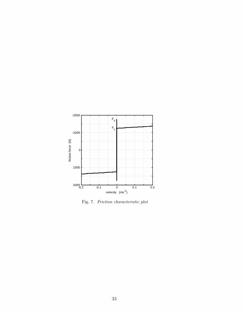
A disadvantage of a physical model of a control valve is that it requires severalparameters to be known. The mass M and typical friction forces depend uponthe design of the valve. Kayihan and Doyle III (2000) used manufacturer’svalues suggested by Fitzgerald (1995) and similar values have been chosenhere apart from a slightly increased value of Fs and a smaller value for Fc inorder to make the demonstration of the slip-jump more obvious (see Table 1).Figure 7 shows the friction force characteristic in which the magnitude of themoving friction is smaller than that of the static friction. The friction forceopposes velocity (see equation 2) thus the force is negative when the velocityis positive.

The calibration factor of Table 1 is introduced because the required stemposition xr is the input to the simulation. In the absence of stiction effectsthe valve moving parts come to rest when the force due to air pressure onthe diaphragm is balanced by the spring force. Thus Au = kx and so thecalibration factor relating air pressure u to xr is k/A. The consequences ofmiscalibration are discussed below.

4.2 Valve simulation

The purpose of simulation of the valve was to determine the influence of thethree friction terms in the model. The non-linearity in the model is able toinduce limit cycle oscillations in a feedback control loop, and the aim is tounderstand the contribution of each friction term to the character and shapeof the limit cycles.

Open Loop response:Figure 8 shows the valve position when the valve model is driven by a si-nusoidal variation in op in open loop in the absence of the controller. Theleft hand column shows the time trends and the right hand panels are plotsof valve demand (op) versus valve position (mv). Several cases are simulatedusing the parameters shown in Table 2. The “linear” values are those sug-gested by Kayihan and Doyle III for the best case of a smart valve with Teflonpacking requiring air pressure of about 0.1 psi (689 Pa) to start it moving.

In the first row of figure 8, the Coulomb friction Fc and static friction Fs aresmall and linear viscous friction dominates. The input and output are almostin phase in the first row of figure 8 because the sinusoidal input is of low

10

frequency compared to the bandwidth of the valve model and is on the partof the frequency response function where input and output are in phase.

Valve deadband is due to the presence of Coulomb friction Fc, a constantfriction which acts in the opposite direction to the velocity. In the deadbandsimulation case the static friction is the same as the Coulomb friction, Fs =Fc. The deadband arises because, on changing direction, the valve remainsstationary until the net applied force is large enough to overcome Fc. Thedeadband becomes larger if Fc is larger.

A valve with high initial static friction such that Fs > Fc exhibits a jumpingbehavior that is different from a deadband, although both behaviors may bepresent simultaneously. When the valve starts to move, the friction force re-duces abruptly from Fs to Fc. There is therefore a discontinuity in the modelon the right hand side of Newton’s second law and a large increase in accel-eration of the valve moving parts. The initial velocity is therefore faster thanin the Fs = Fc case leading to the jump behavior observed in the third rowof figure 8. If the Coulomb friction Fc is absent then the deadband is absentand the slip-jump allows the mv to catch up with the op (fourth row). If thevalve is miscalibrated then swings in the valve position (mv) are larger thanswings in the demanded position (op). In that case the gradient of the op-mvplot is greater than unity during the moving phase. The bottom row of figure8 shows the case when the calibration factor is too large by 25%. A slip-jumpwas also used in this simulation.

Closed loop dynamics:For assessment of closed loop behavior, the valve output drives a first orderplus dead time process G(s) and receives its op reference input from a PIcontroller C(s) where:

G(s) =3e−10s

10s + 1C(s) = 0.2

(10s + 1

10s

)(3)

Figure 9 shows the limit cycles induced in this control loop by the valvetogether with the plots of valve position (mv) versus valve demand (op). Thelimit cycles were present even though the set point to the loop was zero. Thatis, they were internally generated and sustained by the loop in the absence ofany external setpoint excitation.

There was no limit cycle in the linear case dominated by viscous friction or inthe case with deadband only when Fs = Fc. It is known that deadband alonecannot induce a limit cycle unless the process G(s) has integrating dynamics,as will be discussed further in section 5.3.1.

The presence of stiction (Fs > Fc) induces a limit cycle with a characteristictriangular shape in the controller output. Cycling occurs because an offset

11

exists between the set point and the output of the control loop while the valveis stuck which is integrated by the PI controller to form a ramp. By the timethe valve finally moves in response to the controller op signal the actuatorforce has grown quite large and the valve moves quickly to a new positionwhere it then sticks again. Thus a self limiting cycle is set up in the controlloop.

If stiction and deadband are both present then the period of the limit cycleoscillation can become very long. The combination Fs = 1750 N and Fc =1250 N gave a period of 300s while the combination Fs = 1000 N and Fc =400N had a period of about 140s (top row, figure 9), in both cases much longerthan the time constant of the controlled process or its cross-over frequency.The period of oscillation can also be influenced by altering the controller gain.If the gain is increased the linear ramps of the controller output signal aresteeper, the actuator force moves through the deadband more quickly and theperiod of the limit cycle becomes shorter (second row, figure 9). The techniqueof changing the controller gain is used by industrial control engineers to testthe hypothesis of a limit cycle induced by valve non-linearity while the plantis still running in closed loop.

In the pure stick-slip or stiction with no offset case shown in the third rowof figure 9 the Coulomb friction is negligible and the oscillation period isshorter because there is no deadband. The bottom row in figure 9 shows thatmiscalibration causes an overshoot in closed loop.

5 Data driven Model of Valve Stiction

The proposed data driven model has parameters that can be directly related toplant data and it produces the same behavior as the physical model. The modelneeds only an input signal and the specification of deadband plus stickbandand slip jump. It overcomes the main disadvantages of physical modelling of acontrol valve, namely that it requires the knowledge of the mass of the movingparts of the actuator, spring constant, and the friction forces. The effect of thechange of these parameters can not easily be determined analytically becausethe relationship between the values of the parameters and the observation ofthe deadband/stickband as a percentage of valve travel is not straightforward.In a data driven model, the parameters are easy to choose and the effects ofthese parameter change are simple to realize.

12

5.1 Model Formulation

The valve sticks only when it is at rest or it is changing its direction. Whenthe valve changes its direction it comes to a rest momentarily. Once the valveovercomes stiction, it starts moving and may keep on moving for sometimedepending on how much stiction is present in the valve. In this moving phase,it suffers only dynamic friction which may be smaller than the static friction.It continues to do so until its velocity is again very close to zero or it changesits direction.

In the process industry, stiction is generally measured as a % of the valvetravel or the span of the control signal (Gerry and Ruel, 2001). For example,a 2 % stiction means that when the valve gets stuck it will start moving onlyafter the cumulative change of its control signal is greater than or equal to2%. If the range of the control signal is 4 to 20 mA then a 2% stiction meansthat a change of the control signal less than 0.32 mA in magnitude will notbe able to move the valve.

In our modelling approach the control signal has been translated to the per-centage of valve travel with the help of a linear look-up table. In order to handlestochastic inputs, the model requires the implementation of a PI(D) controllerincluding its filter under a full industrial specification environment. Alterna-tively, an EWMA filter (Exponentially Weighted Moving Average) placed rightin front of the stiction model can be used to reduce the effect of noise. Thispractice is very much consistent with industrial practices. The model consistsof two parameters -namely the size of deadband plus stickband S (specified inthe input axis) and slip jump J (specified on the output axis). Note that theterm ‘S’ contains both the deadband and stickband. Figure 10 summarizesthe model algorithm, which can be described as:

• First, the controller output (mA) is provided to the look-up table where itis converted to valve travel %.

• If this is less then 0 or more than 100, the valve is saturated (i.e., fully closeor fully open).

• If the signal is within 0 to 100% range, the algorithm calculates the slopeof the controller output signal.

• Then the change of the direction of the slope of the input signal is takeninto consideration. If the ‘sign’ of the slope changes or remains zero for twoconsecutive instants, the valve is assumed to be stuck and does not move.The ‘sign’ function of the slope gives the following· If the slope of input signal is positive, the sign(slope) returns ‘+1’.· If the slope of input signal is negative, the sign(slope) returns ‘-1’.· If the slope of input signal is zero, the sign(slope) returns ‘0’.

Therefore, when sign(slope) changes from ‘+1’ to ‘-1’ or vice-versa it

13

means the direction of the input signal has been changed and the valve is inthe beginning of its stick position (points A and E in figure 2). The algorithmdetects stick position of the valve at this point. Now, the valve may stickagain while travelling in the same direction (opening or closing direction)only if the input signal to the valve does not change or remains constant fortwo consecutive instants, which is usually uncommon in practice. For thissituation, the sign(slope) changes to ‘0’ from ‘+1’ or ‘-1’ and vice versa. Thealgorithm again detects here the stick position of the valve in the movingphase and this stuck condition is denoted with the indicator variable ‘I ′ = 1.The value of the input signal when the valve gets stuck is denoted as xss.This value of xss is kept in memory and does not change until valve getsstuck again. The cumulative change of input signal to the model is calculatedfrom the deviation of the input signal from xss.

• For the case when the input signal changes its direction (i.e., the sign(slope)changes from ‘+1’ to ‘-1’ or vice versa), if the cumulative change of the inputsignal is more than the amount of the deadband plus stickband (S), the valveslips and starts moving.

• For the case when the input signal does not change the direction (i.e., thesign(slope) changes from ‘+1’ or ‘-1’ to zero, or vice versa), if the cumulativechanges of the input signal is more than the amount of the stickband (J),the valve slips and starts moving. Note that this takes care of the case whenvalve sticks again while travelling in the same direction (EnTech, 1998; Kanoet al., 2004).

• The output is calculated using the equation:

output = input− sign(slope) ∗ (S − J)/2 (4)

and depends on the type of stiction present in the valve. It can be describedas follows:· Deadband: If J = 0, it represents pure deadband case without any slip

jump.· Stiction (undershoot): If J < S, the valve output can never reach the

valve input. There is always some offset. This represents the undershootcase of stiction.

· Stiction (no offset): If J = S, the algorithm produces pure stick-slip be-havior. There is no offset between the input and output. Once the valveovercomes stiction, valve output tracks the valve input exactly. This is thewell-known “stick-slip case”.

· Stiction (overshoot): If J > S, the valve output overshoots the valve inputdue to excessive stiction. This is termed as overshoot case of stiction.

Recall that J is an output (y-axis) quantity. Also, the magnitude of theslope between input and output is 1.

• The parameter, J signifies the slip jump start of the control valve imme-diately after it overcomes the deadband plus stickband. It accounts for theoffset between the valve input and output signals.

14

• Finally, the output is again converted back to a mA signal using a look-uptable based on the valve characteristics such as linear, equal percentage orsquare root, and the new valve position is reported.

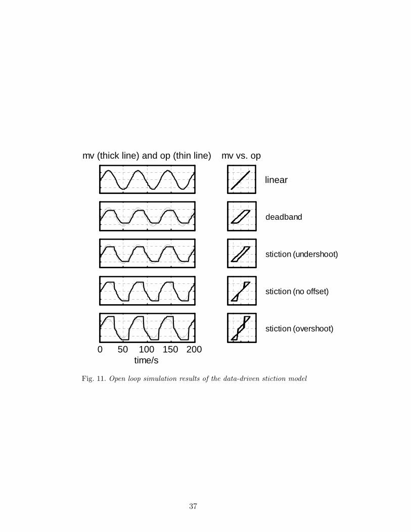
5.2 Open loop response of the model under a sinusoidal input

Figure 11 shows the open loop behavior of the new data-driven stiction modelin presence of various types of stiction. Plots in the left panel show the timetrend of the valve input op (thin solid line) and the output mv (thick solidline). The right panel shows the input-output behavior of the valve on a X-Yplot.

• The first row shows the case of a linear valve without stiction.• The second row corresponds to pure deadband without any slip jump, i.e.,

J = 0. Note that for this case, the magnitude of stickband is zero anddeadband itself equals to ‘S’.

• The third row shows the undershoot case of a sticky valve where J < S.This case is illustrated in the first and second examples of industrial controlloops. In this case the valve output can never reach the valve input. Thereis always some offset.

• The fourth row represents pure stick-slip behavior. There is no offset be-tween the input and output. Once the valve overcomes stiction, valve outputtracks the valve input accurately.

• In the fifth row, the valve output overshoots the desired set position or thevalve input due to excessive stiction. This is termed as overshoot case ofstiction.

In reality a composite of these stiction phenomena may be observed. Althoughthis model is not directly based on the dynamics of the valve, the strength ofthe model is that it is very simple to use for the purpose of simulation and canquantify stiction as a percentage of valve travel or span of input signal. Also,the parameters used in this model are easy to understand, realize and relateto real stiction behavior. Though this is an empirical model and not based onphysics, it is observed that this model can correctly reproduce the behavior ofthe physics-based stiction model. This can be observed by comparing figure12 with 9. The data for these figures are obtained from the simulation of thesame process and controller but with different stiction models. The notablefeatures are:

• For a first order plus time delay model, both stiction model show no limitcycle for the case of pure deadband. Both model show that for limit cyclesa certain amount of slip jump is required.

• Both models show limit cycle even in the presence of pure deadband if the

15

process contains an integrator in closed loop.• Both model produce identical results for other case of stiction.

The open loop simulation results for both models look very similar in figures11 and 8. Note that a one to one comparison of these figures can not be madebecause there is no direct one to one relation among the parameters of theempirical data driven model and that of the physics based model.

5.3 Closed loop behavior of the model

Closed loop behavior of the stiction model has been studied for two differentcases, namely, a concentration loop and a level loop. The concentration loophas slow dynamics with a large dead time. The level loop has only an integra-tor. The transfer functions, controllers and parameters used in simulation areshown in Table 3. The magnitudes of S and J are specified as a percentage(%) of valve input span and output span, respectively. Results are discussedin a separate section for each of the loops.

Concentration loop:The transfer function model for this loop was obtained from (Horch and Isaks-son, 1998). This transfer function with a PI controller in a feedback closed loopconfiguration was used for the simulation. Steady state results of the simu-lation for different stiction cases are presented in figures 12 and 13. In bothfigures thin lines are the controller output. The triangular shape of the timetrend of controller output is one of the characteristics of stiction (Horch, 2000).Note that figure 12 looks really similar to figure 9, for the same process andcontroller but with the physics-based valve model. In all cases, the presence ofstiction causes limit cycling of the process output. In absence of stiction thereare no limit cycles, which is shown in the first row of figure 12. The presenceof pure deadband also does not produce a limit cycle. It only adds dead timeto the process. This conforms with the findings of (McMillan, 1995; Piippo-nen, 1996), where they clearly stated that the presence of pure deadband onlyadds dead time to the process and the presence of deadband together withan integrator produces a limit cycle (discussed further in level control loopcase). Figure 12 shows the controller output (op) and valve position (mv).Mapping of mv vs. op clearly shows the stiction phenomena in the valve. Itis common practice to use a mapping of pv vs. op for valve diagnosis (seefigure 13). However in this case such a mapping only shows elliptical loopswith sharp turn around points. The reason is that the pv-op map captures notonly the nonlinear valve characteristic but also the dynamics of the process,G(s), which in this case is a first order lag plus deadtime. Therefore, if thevalve position data is available one should plot valve position (mv) against thecontroller output (op). The pv-op maps should be used with caution except

16

for in liquid flow low loops where the flow through the valve (pv) can be takento be proportional to valve opening (mv).

A level control loop:The closed loop simulation of the stiction model using only an integrator asthe process was performed to investigate the behavior of a typical level loopin presence of valve stiction. Results are shown in figure 15. The second rowof the figure shows that the deadband can produce oscillations. Again, it isobserved that if there is an integrator in the process dynamics, then even apure deadband can produce limit cycles, otherwise the cycle decays to zero.The mv-op mappings clearly show the various cases of valve stiction. The pv-op plots show elliptical loops with sharp turn around. Therefore, as was notedalso in an earlier example, the pv-op map is not a very reliable diagnostic forvalve faults in a level loop. A diagnostic technique, developed by the authors(Choudhury et al., 2003), based on higher order statistical analysis of data isable to detect and diagnose the presence of stiction in control loops.

6 Describing Function Analysis

6.1 Introduction

A non-linear actuator with a stiction characteristic may cause limit cyclingin a control loop. Further insights into the behaviour of such systems maybe achieved through a describing function analysis (Cook, 1986). The non-linearity is modelled by a non-linear gain N . The assumptions inherent inthe approximation are that there are periodic signals present in the systemand that the controlled system is low pass and responds principally to thefundamental Fourier component. The conditions for oscillation in a negativefeedback loop arise when the loop gain is −1:

Go (iω) = − 1

N (Xm)(5)

where Go (iω) is the open loop frequency response which includes the con-trolled system and the proportional plus integral controller, and N (Xm) isthe describing function which depends on the magnitude of the controlleroutput Xm. When the condition Go(iω) = −1 /N(Xm) is met the systemwill spontaneously oscillate with a limit cycle. The variation of the quantity−1 /N(Xm) with signal amplitude means that signals initially present in theloop as noise can grow until they are big enough to satisfy the equality andhence provide a self-starting oscillation. The solution to the complex equationGo(iω) = −1 /N(Xm), if one exists, may be found graphically by superposingplots of Go (iω) and −1/N on the same set of axes.

17

The aims of describing function analysis are to gain insights into the simulationresults and industrial observations presented in the paper.

6.2 An expression for the describing function

The describing function of a non-linearity is:

N =Yf

X(6)

where X is a harmonic input to the non-linearity of angular frequency ωo andYf is the fundamental Fourier component angular frequency ωo of the outputfrom the non-linearity. Thus a Fourier analysis is needed on the output signalsshown as bold lines in Figure 11. The quantity N depends upon the magnitudeof the input Xm. N is complex for the stiction non-linearity because the outputwaveform has a phase lag compared to the input. The describing function isderived in the appendix where it is shown that:

N = − 1

πXm

(A− iB) (7)

where

A =Xm

2sin 2φ− 2Xm cos φ−Xm

(π

2+ φ

)+ 2 (S − J) cos φ, (8)

B = − 3Xm

2+

Xm

2cos 2φ + 2Xm sin φ− 2 (S − J) sin φ (9)

φ = sin−1(

Xm − S

Xm

)(10)

6.3 Asymptotes of the describing function

Figure 10 indicates that there is no output from the non-linearity if Xm < S/2.Therefore the two extreme cases are when Xm = S/2 and Xm À S.

When Xm À S, then the effects of the deadband and slip-jump are negligibleand the non-linearity in Figure 10 becomes a straight line at 45o. The outputis in phase with the input and N = 1. Thus −1 /N(Xm) = −1 when Xm À S.

In the limit when Xm → S/2 then the output is as shown in Figure 16. The lefthand plot shows the output for a slip-jump with no deadband (S = J, d = 0)while the right hand plot shows a magnified plot of a dead-band with no slip

18

jump (S = d, J = 0). In both cases the output lags the input by one quarterof a cycle. The output is a square wave of magnitude Xm in the S = J, d = 0case and the describing function is N = 4

πe−iπ/2. For the dead-band with no

slip jump (S = d, J = 0) case, the output magnitude becomes very small.The describing function is N = ε e−iπ/2 where ε → 0 as Xm → S/2. Theappendix provides detailed calculations of these results and also shows for thegeneral case that the describing function limit when Xm = S/2 is:

N =4

π× J

2e−iπ/2 (11)

6.4 Insights gained from the describing function

Figure 17 shows graphical solutions to the limit cycle equation Go(iω) =−1 /N(Xm) for the composition control loop (left panel) and level controlloop (right panel) presented earlier. The describing function is parameterizedby Xm and the open loop frequency response function of the controller andcontrolled system is parameterized by ω. Both systems are closed loop stableand thus intersect the negative real axis between 0 and −1. The plots explainthe behavior observed in simulation.

It is clear from the left hand panel of Figure 17 that there will be a limitcycle for the composition control loop if a slip-jump is present. The slip-jumpforces the −1/N curve onto the negative imaginary axis in the Xm = S/2limit. Thus the frequency response curve of the FOPTD composition loopand its proportional plus integral controller, is guaranteed to intersect withthe describing function because the integral action means open loop phase isalways below −π/2 (i.e. it is in the third quadrant of the complex plane atlow frequency).

The figure also shows the −1/N curve for the deadband limit cycle. In theXm = S/2 limit the curve becomes large, negative and imaginary. The compo-sition loop does not have a limit cycle if the non-linearity is a pure deadband,because the frequency response curve does not intersect the −1/N curve. Thelack of a limit cycle in this case has been noted by other authors (McMillan,1995; Piipponen, 1996).

The level loop with proportional plus integral control has a frequency responsefor which the phase becomes −π at low frequency. The right hand panel ofFigure 17 shows that it will intersect the −1/N curves for the slip-jump casesand also for the pure deadband case. Therefore a valve with a deadband andno slip-jump can cause a limit cycle oscillation for an integrating processwith a P+I controller. The frequency of oscillation is higher and the periodof oscillation shorter when the slip-jump is present because the −1/N curves

19

with the slip-jump intersect the frequency response curve at higher frequenciesthan the −1/N curve for the deadband.

The above insights from describing function analysis indicate that for onlinecompensation of stiction it can be beneficial to use a PI controller where theintegral action has a variable strength (Gerry and Ruel, 2001). If absolute error(sp-pv) is smaller than some value then take out the integral action, otherwiseuse it. For example, if error is less than some value (say, x), then ki = 0, if not,ki = normalvalue, where ki is the integral constant of the controller. Usingthis method, when the valve is within the stiction band, the integral is missingfrom the controller. The controller output will not integrate having the endof removing the stiction cycle from the loop. Alternatives are special controlalgorithms that identify and compensate for the friction characteristics of thevalve for instance as described in (Armstrong-Helouvry et al., 1994; Hatipogluand Ozguner, 1998; Kayihan and Doyle III, 2000; Hagglund, 2002; Tao etal., 2002).

7 Conclusion

A generalized definition of valve stiction based on the investigation of the realplant data has been proposed. Since the physics-based model of stiction isdifficult to use because of the requirement of knowledge of mass and forces, asimple yet powerful data-driven empirical stiction model has been developed.Both closed and open loop results have been presented and validated to showthe capability of the model. It is recommended that when using a X-Y plot toanalyze valve problems one should use mv-op plot instead of pv-op.

8 Acknowledgements

Financial support to the first author in the form of a Canadian Interna-tional Development Agency (CIDA) scholarship is gratefully acknowledged.The project has also been supported by the Natural Sciences and Engineer-ing Research Council of Canada (NSERC), Matrikon Consulting Inc., and theAlberta Science and Research Authority (ASRA) in the form of an NSERC-Matrikon-ASRA Industrial Research Chair Program at the University of Al-berta. The authors are also grateful to BP Amoco Oil Ltd. and Tech-ComincoInc. in Trail, B.C., Canada for permitting us to use their data.

20

A APPENDIX – OUTLINE DERIVATION OF DESCRIBINGFUNCTION

A.1 Expression for the output of the non-linearity

The output from the stiction non-linearity (e.g. the bold trend in the thirdpanel of Figure 11) is not analytic. It is convenient to consider a sine waveinput with angular frequency of 1 rad · s−1 and period 2π. The output then is:

y (t) =

k(Xm sin (t)− S−J

2

)0 6 t 6 π

2

k(Xm − S−J

2

)π2

6 t 6 π − φ

k(Xm sin (t) + S−J

2

)π − φ 6 t 6 3π

2

k(−Xm + S−J

2

)3π2

6 t 6 2π − φ

k(Xm sin (t)− S−J

2

)2π − φ 6 t 6 2π

where Xm is the amplitude of the input sine wave, S is the deadband plusstickband, J is the slip-jump, φ = sin−1

(Xm−S

Xm

)and k is the slope of the

input-output characteristic in the moving phase (k = 1 is assumed for a valve).

A.2 Evaluation of the fundamental Fourier component

The fundamental component of the complex Fourier series is:

1

2π

2π∫

t=0

y (t) e−itdt

where, after substitution of sin (t) = 12i

(e it − e−it):

2π∫

t=0

y (t) e−itdt =

π/2∫

t=0

k(

Xm

2i

(e it − e−it

)− S − J

2

)e−itdt +

π−φ∫

t=π/2

k(Xm − S − J

2

)e−itdt

+

3π/2∫

t=π−φ

k(

Xm

2i

(e it − e−it

)+

S − J

2

)e−itdt +

2π−φ∫

t=3π/2

k(−Xm +

S − J

2

)e−itdt

+

2π∫

t=2π−φ

k(

Xm

2i

(e it − e−it

)− S − J

2

)e−itdt (A-1)

21

Writing it compactly:

2π∫

t=0

y (t) e−itdt = T1 + T2 + T3 + T4 + T5

where T1 =π/2∫t=0

k(

Xm

2i(e it − e−it)− S−J

2

)e−itdt , and so on.

Evaluation term by term gives:

T1 =k

2(Xm − S + J) + ik

(S − J

2− aπ

4

)

T2 =−k(Xm − S − J

2

)(1− sin φ)− ik

(Xm − S − J

2

)cos φ

T3 = k(

Xm

4(1 + cos 2φ)− S − J

2(1 + sin φ)

)+ ik

(Xm

4sin 2φ− Xm

2

(π

2+ φ

)+

S − J

2cos φ

)

T4 =−k(Xm − S − J

2

)(1− sin φ)− ik

(Xm − S − J

2

)cos φ

T5 =−k(

Xm

4(1− cos 2φ) +

S − J

2sin φ

)− ik

(Xmφ

2+

d

2− Xma

4sin 2φ− S − J

2cos φ

)(A-2)

Collecting terms gives the wanted fundamental Fourier component of the out-put:

12π

2π∫t=0

y (t) e−itdt = 12π

(B + iA)

where A =(kXm

2sin 2φ− 2kXm cos φ− kXm

(π2

+ φ)

+ 2k (S − J) cos φ)

and B = −3kXm

2+ kXm

2cos 2φ + 2kXm sin φ− 2k (S − J) sin φ

The fundamental component of the complex Fourier series of the input sinewave is Xm/2i. Therefore the describing function is:

N =B + iA

2π× 2i

Xm

= − 1

πXm

(A− iB)

A.3 Evaluation of limiting cases

There is no output from the non-linearity when Xm < S/2. The limiting casesconsidered are therefore Xm = S/2 and Xm À S.

When Xm À S then φ = sin−1(

Xm−SXm

)= π

2, A = −kπXm, B = 0 and thus

N = k. This result is to be expected because the influence of the stickband

22

and jump are negligible when the input has a large amplitude and the outputapproximates a sinewave of magnitude kXm. The slope of the moving phasefor a valve with a deadband is k = 1 when the input and output to the non-linearity are expressed as a percentage of full range. Therefore for a valve withstiction, N = 1, when Xm À S.

When Xm = S/2 the result depends upon the magnitude of the slip-jump,J . For the case with no deadband (S = J), φ = −π

2, A = 0, B = −4kXm

and N = −ik 4π

= k 4πe−iπ/2. For a valve with k = 1, N = 4

πe−iπ/2. This result

describes the situation where the output is a square wave of amplitude Xm

lagging the input sine wave by one quarter of a cycle, as shown in Figure 16.

For intermediate cases where both deadband and slip jump are present suchthat |S − J | > 0, then the Xm = S/2 limit gives φ = −π

2, A = 0, B = −2kJ

and N = −ik 2JπXm

= k 2JπXm

e−iπ/2. For instance, if J = S/2 and k = 1 then

the Xm = S/2 limit gives N = 2πe−iπ/2 and the output is a square wave of

amplitude Xm/2 lagging the input sine wave by one quarter of a cycle.

When the non-linearity has a deadband only and no slip-jump (J = 0) thedescribing function has a limit given by N = εe−iπ/2 where ε → 0 as Xm →S/2.

23

References

Armstrong-Helouvry, Brian, Pierre Dupont and Carlos C. De Wit (1994). A surveyof models, analysis tools and compensation methods for the control of machineswith friction. Automatica 30(7), 1083–1138.

Aubrun, C., M. Robert and T. Cecchin (1995). Fault detection in control loops.Control Engineering Practice 3, 1441–1446.

Bialkowski, W. L. (1992). Dreams vs. reality: A view from both sides of the gap.In: Control Systems. Whistler, BC, Canada. pp. 283–294.

Choudhury, M. A. A. S., Sirish L. Shah and Nina F. Thornhill (2003). Diagnosisof poor control loop performance using higher order statistics. accepted forpublication in Automatica, June 2003.

Cook, P. A. (1986). Nonlinear Dynamical Systems. Prentice-Hall International.London.

Desborough, L. and R. Miller (2002). Increasing customer value of industrial controlperformance monitoring - honeywell’s experience. In: AIChE Symposium Series2001. number 326. pp. 172–192.

Ender, D. (1993). Process control performance: Not as good as you think. ControlEngineering 40, 180–190.

EnTech (1998). EnTech Control Valve Dynamic Specification (version 3.0).

Fisher-Rosemount (1999). Control Valve Handbook. Fisher Controls International,Inc. Marshalltown, Iowa, USA.

Fitzgerald, Bill (1995). Control Valve for the Chemical Process Industries. McGraw-Hill, Inc. New York.

Gerry, John and Michel Ruel (2001). How to measure and combat valve stictiononline. Instrumetnation, Systems and Automated Society. Houston, Texas,USA. http://www.expertune.com/articles/isa2001/StictionMR.htm.

Hagglund, T. (2002). A friction compensator for pneumatic control valves. Journalof Process Control 12(8), 897–904.

Hatipoglu, C. and U. Ozguner (1998). Robust control of systems involving non-smooth nonlinearities using modifed sliding manifolds. Philadelphia, PA.pp. 2133–2137. American control conference.

Horch, A. and A. J. Isaksson (1998). A method for detection of stiction in controlvalves. In: Proceedings of the IFAC workshop on On line Fault Detection andSupervision in the Chemical Process Industry. Session 4B. Lyon, France.

Horch, A., A. J. Isaksson and K. Forsman (2000). Diagnosis and characterizationof oscillations in process control loops. In: Proceedings of the Control Systems2000. Victoria, Canada. pp. 161–165.

24

Horch, Alexander (2000). Condition Monitoring of Control Loops. PhD thesis. RoyalInstitute of Technology. Stockholm, Sweden.

ISA Subcommittee SP75.05 (1979). Process instrumentation terminology. TechnicalReport ANSI/ISA-S51.1-1979. Instrument Society of America.

Kano, Manabu, Hiroshi Maruta, Hidekazu Kugemoto and Keiko Shimizu (2004).Practical model and detection algorithm for valve stiction. In: to appear in theProceedings of the 7th DYCOPS. Boston, USA.

Karnopp, Dean (1985). Computer simulation of stic-slip friction in mechanicaldynamical systems. Journal of Dynamic Systems, Measurement, and Control107, 420–436.

Kayihan, Arkan and Francis J. Doyle III (2000). Friction compensation for a processcontrol valve. Control Engineering Practice 8, 799–812.

Martin, G. D., L.E. Turpin and R. P. Cline (1991). Estimating control functionbenefits. Hydrocarbon Processing pp. 68–73.

McMillan, G. K. (1995). Improve control valve response. Chemical EngineeringProgress: Measurement and Control pp. 77–84.

Miao, Tina and Dale E. Seborg (1999). Automatic detection of excessively oscillatorycontrol loops. In: Proceedings of the 1999 IEEE International Conference onControl Applications. Kohala Coast-Island of Hawai’i, Hawai’i, USA.

Olsson, H. (1996). Control Systems with Friction. PhD thesis. Lund Institute ofTechnology. Sweden.

Paulonis, Michael A. and John W. Cox (2003). A practical approach for large-scale controller performance assessment, diagnosis, and improvement. Journalof Process Control 13(2), 155–168.

Piipponen, Juha (1996). Controlling processes with nonideal valves: Tuning of loopsand selection of valves. In: Control Systems. Chateau, Halifax, Nova Scotia,Canada. pp. 179–186.

Qin, S. J. (1998). Control performance monitoring - a review and assessment.comput. chem. eng. 23, 173–186.

Ruel, Michel (2000). Stiction: The hidden menace. Control Magazine.http://www.expertune.com/articles/RuelNov2000/stiction.html.

Sharif, M. A. and R. I. Grosvenor (1998). Process plant condition monitoring andfault diagnosis. Proc Instn Mec Engrs 212(Part E), 13–30.

Shinskey, F. G. (1990). How good are our controllers in absolute performance androbustness. Measurement and Control 23, 114–120.

Taha, Othman, Guy A. Dumont and Michael S. Davies (1996). Detection anddiagnosis of oscillations in control loops. In: Proceedings of the 35th conferenceon Decision and Control. Kobe, Japan.

25

Tao, Gang, Shuhao Chen and Suresh m. Joshi (2002). An adaptive control schemefor systems with unknown actuator failures. Automatica 38, 1027–1034.

Thornhill, N. F., B. Huang and H. Zhang (2003a). Detection of multiple oscillationsin control loops. Journal of Process Control 13, 91–100.

Thornhill, N. F., F. Cox and M. Paulonis (2003b). Diagnosis of plant-wide oscillationthrough data-driven analysis and process understanding. Control Engng. Prac.11(12), 1481–1490.

Wallen, Anders (1997). Valve diagnostics and automatic tuning. In: Proceedings ofthe American Control Conference. Albuquerque, New Mexico. pp. 2930–2934.

Whalen, Bruce R. (1983). Basic Instrumentation. 3 ed.. Petroleum ExtensionService (PETEX). Austin, TX.

26

input

outp

ut

hysteresis

a

(a) hysteresisinput

outp

ut

deadbandb

(b) deadband

input

outp

ut

hysteresis + deadband

(c) hysteresis + deadbandinput

outp

ut

d

(d) deadzone

deadzone

deadbandb

input

outp

ut

hysteresis

a

(a) hysteresisinput

outp

ut

hysteresis

a

(a) hysteresisinput

outp

ut

deadbandb

deadbandb

(b) deadband

input

outp

ut

hysteresis + deadband

(c) hysteresis + deadbandinput

outp

ut

d

(d) deadzone

deadzone

input

outp

ut

d

(d) deadzone

deadzone

deadbandb

Fig. 1. Hysteresis, Deadband, and Deadzone (redrawn from ANSI/ISA-S51.1-1979)

27

valv

e o

utp

ut (

man

ipul

ated

var

iab

le)

valve input (controller output)

deadband stickband

slip jump, J

stickband + deadband = S

mov

ing

phas

e

A BC

D

EF

G

valv

e o

utp

ut (

man

ipul

ated

var

iab

le)

valve input (controller output)

deadband stickband

slip jump, J

stickband + deadband = S

mov

ing

phas

e

A BC

D

EF

G

Fig. 2. Typical input-output behavior of a sticky valve

28

0 100 200

-1.5

-1

-0.5

0

0.5

1

1.5

sampling instants

pv a

nd o

p

-1 0 1

-1

0

1

controller output, op

proc

ess o

utpu

t, pv

0 100 200

-1.5

-1

-0.5

0

0.5

1

1.5

sampling instants

mv a

nd o

p

-1 0 1

-1

0

1


valve

pos

ition,

mv

A A A A

A A A A

Fig. 3. Flow control cascaded to level control in an industrial setting, the line withcircles is pv and mv, the thin line is op

29

0 200 400

-1

0

1

sampling instants

pv a

nd o

p

-1 0 1

-1

0

1


proc

ess

outp

ut, p

v

A

A

A A

A A A

A

Fig. 4. Data from a flow loop in a refinery, time trend of pv and op (left) - the linewith circles is pv and the thin line is op, and the pv-op plot (right)

30

0 100 200 300 400

-1

0

1

sampling instants

pv a

nd o

p

-1 0 1

-1

0

1

controller output, oppr

oces

s ou

tput

, pv

0 100 200 300 400

-1

0

1

sampling instants

pv a

nd s

p

-1 0 1

-1

0

1

set point, sp

proc

ess

outp

ut, p

v

A

A

A

A

A

A

A

A

A

A

A

Fig. 5. Data from a flow loop in a refinery, time trend of pv and op (top left) - theline with circles is pv and the thin line is op, the pv-op plot(top right), time trendof pv and sp (bottom left), line with circles is pv and thin line is sp, and the pv-spplot(bottom right)

31

0 200 400

-2

-1

0

1

2

pv a

nd o

p

-2 -1 0 1 2

-2

-1

0

1

2

op

pv

0 200 400

-2

-1

0

1

2

sampling instants

flow

rate

and

op

-2 -1 0 1 2

-2

-1

0

1

2


flow

rate

Fig. 6. Industrial dryer temperature control loop data, lines with circles are pv andflowrate, the thin line is op (the bottom left panel)

32

-0.2 -0.1 0 0.1 0.22000

1000

0

-1000

-2000

velocity (ms-1)

fric

tion

forc

e (

N)

Fs

Fc

-

-

Fig. 7. Friction characteristic plot

33

mv (thick line) and op (thin line)

0 50 100 150 200time/s

mv vs. op

linear

pure deadband

stiction (undershoot)

stiction (no offset)

stiction (overshoot)

Fig. 8. Open loop response of mechanistic model. The amplitude of the sinusoidalinput is 10 cm in each case.

34


0 100 200 300time/s


mv vs. op


PI gain doubled



Fig. 9. Closed loop response of mechanistic model

35

y(k)=y(k-1)

v_new=[x(k)-x(k-1)]/∆∆∆∆t

x(k)<100

x(k)>0

no

xss=x(k-1)y(k)=y(k-1)

no

Valve sticks

Valve characteristics (e.g., linear, square root, etc.)(Converts valve % to mA)

x(k)

xss=xssy(k)=0

xss=xssy(k)=100

yes

Look up table(Converts mA to valve %)

no

mv(k)

y(k)

|x(k)-xss|>S

yes

sign (v_new)=sign(v_old)

yes

yes

y(k)=x(k) - sign(v_new)*(S-J)/2

Valve slips and moves

op(k)

no

remain stuck

sign(v_new)=0

I = 1 ?

no

no

|x(k)-xss|>JI = 1

I = 0

no

yesyes

yes

y(k)=y(k-1)

v_new=[x(k)-x(k-1)]/∆∆∆∆t

x(k)<100

x(k)>0 x(k)>0

no

xss=x(k-1)y(k)=y(k-1)xss=x(k-1)y(k)=y(k-1)

no

Valve sticks

Valve characteristics (e.g., linear, square root, etc.)(Converts valve % to mA)

x(k)

xss=xssy(k)=0xss=xssy(k)=0

xss=xssy(k)=100xss=xssy(k)=100

yes

Look up table(Converts mA to valve %)

no

mv(k)mv(k)

y(k)

|x(k)-xss|>S

yes

sign (v_new)=sign(v_old)sign (v_new)=sign(v_old)

yes

yes

y(k)=x(k) - sign(v_new)*(S-J)/2

Valve slips and moves

op(k)op(k)

no

remain stuck

sign(v_new)=0

I = 1 ?

no

no

|x(k)-xss|>JI = 1

I = 0

no

yesyes

yes

Fig. 10. Signal and logic flow chart for the data-driven stiction model

36


0 50 100 150 200time/s

mv vs. op

linear

deadband




Fig. 11. Open loop simulation results of the data-driven stiction model

37


0 100 200 300time/s

mv vs. op

linear

pure deadband




Fig. 12. Closed loop simulation results of a concentration loop in presence of thedata-driven stiction model

38

pv (thick line) and op (thin line)

0 100 200 300time/s

pv vs. op

linear

pure deadband




Fig. 13. Closed loop simulation results of a concentration loop in presence of thedata-driven stiction model

39


0 100 300 500time/s

mv vs. op

linear

pure deadband




Fig. 14. Closed loop simulation results of a level loop in presence of the data-drivenstiction model

40

pv (thick line) and op (thin line)

0 100 300 500time/s

pv vs. op

linear

pure deadband




Fig. 15. Closed loop simulation results of a level loop in presence of the data-drivenmodel

41

0 ππππ /2 ππππ 3ππππ /2 2ππππtime/sin

put (

thin

line

) and

out

put (

heav

y lin

e)


put (

thin

line

) and

out

put (

heav

y lin

e)


put (

thin

line

) and

out

put (

heav

y lin

e)


put (

thin

line

) and

out

put (

heav

y lin

e)

Fig. 16. Input (thin line) and output (heavy line) time trends for the limiting case asXm = S/2. Left panel: Slip-jump only with S = J . Right panel: Deadband only withJ = 0. The output in the left plot has been magnified for visualization; its amplitudebecomes zero as Xm approaches S/2.

42

−3 −2 −1 0 1−5

−4

−3

−2

−1

0

1im

agin

ary

axis

real axis

J = S

J = S/3J = S/5

J = 0

G(iω)−3 −2 −1 0 1

−5

−4

−3

−2

−1

0

1

real axis

J = S

J = S/3

J = S/5

J = 0

G(iω)

Fig. 17. Graphical solutions for limit cycle oscillations. Left panel: Compositioncontrol loop. Right panel: level control loop. Dotted lines are the −1/N curves andthe solid line is the frequency response function.

43

Table 1Nominal values used for physical valve simulation

Parameters Kayihan and Doyle III, 2000 Nominal case

M 3 lb (1.36 kg) 1.36 kg

Fs 384 lbf (1708 N) 1750 N

Fc 320 lbf (1423 N) 1250 N

Fv 3.5 lbf.s.in−1 (612 N.s.m−1) 612 N.s.m−1

spring constant, k 300 lbf.in−1 (52500 N.m−1) 52500 N.m−1

diaphragm area, A 100 in2 (0.0645 m2) 0.0645 m2

calibration factor, k/A - 807692 Pa.m−1

air pressure 10 psi (68950 Pa) 68950 Pa

44

Table 2Friction values used in simulation of physical valve model

stiction

Parameters linear deadband undershoot no offset

open loop closed loop

Fs (N) 45 1250 2250 1000 1750

Fc (N) 45 1250 1250 400 0

Fv (N.s.m−1) 612 612 612 612 612

45

Table 3Process Model and Controller Transfer, and parameter values used for closed loopsimulation of the data-driven model.

stiction

Loop Type Process Controller deadband undershoot no offset overshoot

S J S J S J S J

concentration 3e−10s

10s+1 0.2(10s+110s ) 5 0 5 2 5 5 5 7

Level 1s 0.4(2s+1

2s ) 3 0 3 3.5 3 3 3 4.5

46

Documents

Modelling Valve Stiction 1 - University of Alberta