Actuator Stiction Compensation via Model Predictive

Actuator Stiction Compensation via Model Predictive Controlfor Nonlinear Processes

Helen DurandDept. of Chemical and Biomolecular Engineering, University of California, Los Angeles, CA 90095-1592

Panagiotis D. ChristofidesDept. of Chemical and Biomolecular Engineering, University of California, Los Angeles, CA 90095-1592

Dept. of Electrical Engineering, University of California, Los Angeles, CA 90095-1592

DOI 10.1002/aic.15171Published online February 13, 2016 in Wiley Online Library (wileyonlinelibrary.com)

The problem of valve stiction is addressed, which is a nonlinear friction phenomenon that causes poor performance ofcontrol loops in the process industries. A model predictive control (MPC) stiction compensation formulation is devel-oped including detailed dynamics for a sticky valve and additional constraints on the input rate of change and actuationmagnitude to reduce control loop performance degradation and to prevent the MPC from requesting physically unrealis-tic control actions due to stiction. Although developed with a focus on stiction, the MPC-based compensation methodpresented is general and has potential to compensate for other nonlinear valve dynamics which have some similaritiesto those caused by stiction. Feasibility and closed-loop stability of the proposed MPC formulation are proven for a suffi-ciently small sampling period when Lyapunov-based constraints are incorporated. Using a chemical process examplewith an economic model predictive controller (EMPC), the selection of appropriate constraints for the proposed methodis demonstrated. The example verified the incorporation of the stiction dynamics and actuation magnitude constraints inthe EMPC causes it to select set-points that the valve output can reach and causes the operating constraints to be met.VC 2016 American Institute of Chemical Engineers AIChE J, 62: 2004–2023, 2016

Keywords: model predictive control, valve dynamics, chemical processes, process control, economic model predictivecontrol, stiction

Introduction

Model predictive control (MPC) is a popular optimization-based control method in the chemical process industries and asa result, has received extensive academic research attention,with many variants developed to address the range of goalsthat industry may have. A commonality between all of theMPC strategies is that they require a sufficiently accurate pro-cess model for good performance. This process model shouldinclude significant dynamics of the process, including those ofthe valves if they cannot be assumed to be instantaneous.However, although valve dynamics, particularly nonlinearvalve dynamics such as stiction and backlash, often causepoor performance of control loops in industry,1,2 valve dynam-ics are seldom incorporated in developments in MPC.

Valve stiction is a phenomenon caused by friction betweenvalve components and refers to the tendency of a valve not tomove upon the change of the control signal sent to the valveuntil the control signal exceeds a certain threshold, at whichtime there may be a sudden movement of the valve compo-nents causing the valve output (i.e., process manipulatedinput) to change quickly. The percentage of the available

range of valve outputs traversed when the valve output

changes quickly quantifies the phenomenon of slip-jump.

When the valve is moving (in the moving phase), the valve

output typically is linearly related to the valve input until the

changes in the valve input change sign (i.e., the valve input

begins to decrease when it was previously increasing, or vice

versa), at which point the valve begins to stick again. Because

stiction has been characterized in various ways by different

authors, the authors of Ref. 3 compile some of the stiction def-

initions, ending with the definition determined by the authors

based on observations of plant data, which classifies stiction as

a friction effect that manifests itself through a sudden change

in the valve output in response to a changing input signal. Spe-

cifically, the authors of Ref. 3 define four major regimes in the

dynamic response of the control valve output to changes in the

input to the valve determined by the controller: deadband,

stickband, slip-jump, and the moving phase. In the absence of

slip-jump, only deadband (i.e., the percentage of the available

range of the input signals to the valve throughout which the

valve output does not change in the absence of slip-jump) and

the moving phase exist. When a valve experiences slip-jump,

the valve remains stuck throughout the deadband and also

throughout a percentage of the available range of inputs

beyond the deadband (called the stickband) until it slips from

the value at which it was stuck to a value in the moving phase.

Correspondence concerning this article should be addressed to P. D. Christofidesat [email protected].

VC 2016 American Institute of Chemical Engineers

2004 AIChE JournalJune 2016 Vol. 62, No. 6

Stiction has posed a significant issue in chemical processcontrol throughout the last several decades. Reports from the

1990s indicated that stiction negatively affected control loopperformance at the time,4,5 and a report from Honeywell indi-cated that when studying 26,000 proportional-integral-

derivative (PID) controllers, the performance of about one-thirdwas classified in the lowest of the classification categories(“poor” and “fair”), with valve issues, including stiction, caus-

ing about one-third of these low classifications.1 More recently,Ref. 6 cited stiction as a contributor to plantwide oscillationsand included plant data from the Mitsubishi Chemical Corpora-

tion for a plant where stiction contributed to plantwide oscilla-tions. In addition, in Ref. 7, the proposed stiction detection andquantification method is performed on industrial data for plants

with sticky valves, demonstrating that the problem of valve stic-tion remains a challenging one. As a result, a significant levelof research has been performed throughout the years in an

attempt to more accurately model, detect, quantify, and combatstiction (see the review paper Ref. 8 for a general overview of

stiction modeling, detection, quantification, and compensation).The physical cause of stiction in control valves is best

explained using a specific valve type for clarity of presentation,but the same basic principles will hold for other valve types as

well. For example, a pneumatic spring-diaphragm sliding-stemglobe valve has a valve stem that, in response to a pressureapplied to a diaphragm, moves to adjust the valve output. In a

valve with stiction, the valve output may not approach the valuerequested due to friction forces between the valve stem and thepacking that can prevent the valve stem from moving to the

required position until the pressure applied to the valve dia-phragm is large enough to overcome the breakaway force forthe packing-stem contact. The cause of friction between the

valve stem and the packing is that the materials from which thestem and packing are made are rough at a microscopic level,

with protrusions called asperities. The interactions of the asper-ities on the two surfaces result in friction forces.9 The frictionphenomenon is often described using static, Coulomb, and

viscous friction, as well as the Stribeck effect. However, thereare a number of other phenomena that result from friction,including rising static friction, presliding displacement (micro-

slip), frictional memory in sliding, stick-slip,9 hysteresis withnonlocal memory during presliding,10 velocity weakening, thelift-up effect,11 and asymmetric stiction.12

Friction models have been developed throughout the years

that model these friction effects to varying degrees. For exam-ple, the Classical4,13 model only accounts for the Coulomband viscous forces and the Stribeck effect in the sliding

regime, representing any presliding dynamics with a staticfriction force. As models were developed throughout time,

such as the Dahl,14,15 LuGre,16 Leuven,10,17 Elasto-Plastic,18

and generalized Maxwell-Slip19 models, they began to incor-porate some of the more subtle friction effects in both the pre-

sliding and sliding regimes. A generic model that attempted torepresent the known friction dynamics by modeling variousinteractions between asperities was also developed.11 A num-

ber of researchers have also developed algorithm-based empir-ical friction models, known as data-driven models, thatattempt to represent friction dynamics using decision tree

structures. This class of models includes the Stenman,20

Choudhury,3 Kano,21 and He22 models.A number of works utilizing friction models in control strat-

egies to counter friction have examined adapting friction

model parameters.23–25 In addition, the parameters of the fric-

tion model change with time for a valve as stiction worsensover time, which may occur for reasons such as tightening of

the valve packing or degradation or depletion of materials thatcomprise or lubricate the valve.26,27 For example, in Refs. 4and 5, it is seen that as stiction worsens in a pneumatic

sliding-stem globe valve, the range of stem positions that canbe reached with a given range of pressures applied to the valveis reduced. This is significant because the pressure available to

be applied to a valve is limited,28 with the result that as stic-tion worsens, the given range of pressures cannot move thevalve stem as significantly as when stiction was minimal. This

shows that a negative effect of stiction is that it changes thevalve dynamics and in effect constrains the range of valve out-puts available for a given range of actuation magnitudes.

Other negative effects of stiction include set-point tracking

issues and oscillations in control loops that result from dead-band/stickband and slip-jump. For example, when a valve has

deadband/stickband, the valve output does not change inresponse to changes in the control signal to the valve until thecontrol signal overcomes the deadband/stickband, which pre-

vents the valve output from tracking its set-point. Oscillationscan occur in a control loop with integral action and a valvewith deadband/stickband and slip-jump due to effects similar

to those caused by wind-up in an integrating controller. Ifthere is significant deadband/stickband before the valve slipsand the valve controller is aggressive, the integral action

becomes large, and although it may be desirable to stop thevalve from moving or to move it in the opposite direction soonafter it slips, the integral action of the controller causes it to

continue moving in the original direction for some time,resulting in overshoot of the set-point and possibly oscillationsas occurs in the case of controller wind-up.29 In addition, slip-

jump is known to contribute to oscillatory behavior.7

A good deal of work has been performed to reduce the nega-tive effects of stiction on engineering processes. As mentioned

above with respect to adapting friction model parameters, anumber of methods have been developed to reduce the trackingoffset that can result from friction (many appear in the literature

for high-precision mechanical applications such as machining)using control laws based on a friction model (see, e.g., Refs. 5and 30). Much of the stiction compensation literature for sticky

valves in chemical plant control loops has focused on reducingoscillations. Methods for oscillation reduction include theknocker and variations upon it26,27,31,32 and the constant rein-

forcement method of Ref. 29, which add signals to the control-ler output to reduce the amplitude of oscillations in the processvariable that is controlled by manipulating the valve output.

Other methods include the two moves method and its exten-sions,33–35 which attempt to drive the valve stem to a specific

position, an optimization method33 which can compute com-pensating signals to add to controller outputs to minimize unde-sirable effects of stiction compensation such as excessive stem

movement, and retuning methods.36–38

An observation is that the stiction compensation literaturefor oscillating control loops often refers to processes in whichthe process variable controlled by the valve output is measured

and fed back to a controller. Because the deadband/stickbandmay cause the valve dynamics to act like a time delay in thecontrol loop in such a case, and time delays in a control loop

are known to cause oscillations, this effect may contribute tothe oscillations observed in some cases; however, although thecontrol architecture used to control a sticky valve may have an

impact in some cases on the poor performance of a control

AIChE Journal June 2016 Vol. 62, No. 6 Published on behalf of the AIChE DOI 10.1002/aic 2005

loop, it can often be the deadband/stickband combined withslip-jump, rather than the control architecture, that causes thelimit cycle behavior observed in numerous control loops con-taining sticky valves.

In addition to the stiction compensation methods men-tioned above, predictive control methods have also beenlooked at for stiction compensation. In Ref. 39, a predictivecontroller for applications requiring high precision ofmechanical movement was augmented by time delay con-trol and zero phase error tracking control to improve itstracking performance in the presence of nonlinear frictioneffects. Nonlinear MPC is used in Ref. 40 to control ahydraulic actuator subject to constraints. In Ref. 41, MPCand a deadzone compensator are used to control a gantrycrane subject to deadzone and saturation. In Ref. 42, aninverse backlash model and valve saturation are incorpo-rated in an MPC for linear systems to overcome the dead-band associated with backlash, and this controller isapplied to a system with stiction in Ref. 43. In Ref. 44, thebounds on the optimization variables computed by an MPCare adjusted based on the knowledge that the MPC is inseries with a unit that applies the inverse model for dead-zone, stiction, or backlash to the output from the MPC andsends this signal to a valve with nonlinear dynamics thatcan saturate.

In this work, we propose MPC incorporating stictiondynamics, actuation magnitude constraints, and input rate ofchange constraints as a stiction compensation strategy for non-linear process systems. We use a control architecture thatavoids potential oscillation issues caused by delays in controlloops and develop a process-valve dynamic model to be incor-porated in MPC that includes detailed dynamics for a valvewith stiction. We suggest a number of variations to the costfunction and constraints of the proposed MPC such that it canbe formulated to alleviate set-point tracking errors and oscilla-tions due to stiction for a variety of cases. We further elucidatethe need for actuation magnitude constraints in the proposedMPC to ensure that the set-points calculated by the controllerremain physically reachable as stiction worsens. With theaddition of Lyapunov-based stability constraints and a suffi-ciently small sampling period, the proposed controller is pro-ven to be recursively feasible and to ensure closed-loopstability of the nonlinear process-valve system. Through achemical process example, we motivate the addition of actua-tion magnitude constraints to MPC for stiction compensationand demonstrate the improvement in the set-point trackingability of valves when the actuator dynamics and actuationmagnitude constraints are incorporated in MPC compared tothe case when they are not. The focus of the discussion is oncompensating for stiction in control loops; however, the pro-posed method is flexible and could be examined as a compen-sating strategy for other valve nonlinearities as well. Althoughthe technique of incorporating valve dynamics in MPC toimprove control performance is similar to the approach in Ref.45, which demonstrated that for a linear actuator layer, theincorporation of actuator dynamics in economic model predic-tive control (EMPC) can be important for ensuring that pro-cess constraints are satisfied, this work significantly extendsthe concepts of that work to compensate directly for the non-linear dynamics of stiction. Specifically, it develops additionalconstraints that should be considered for use in MPC whenvalves are known to have stiction in order to compensate forits effects, and the results impact all variants of MPC, ratherthan EMPC only.

Preliminaries

Notation

In this work, tk5kD; k50; 1; 2; . . . refers to synchronoustime instants separated by a sampling period D. The Euclideannorm of a vector is denoted by j � j. A function a : ½0; aÞ ! ½0;1Þ with að0Þ50 belongs to class K if it is continuous andstrictly increasing. A level set of a scalar-valued positivedefinite function V(x) is defined to be the setXq : 5fx 2 Rn jVðxÞ � qg. Set subtraction is denoted using“/” (i.e., x 2 A=B : 5fx 2 Rn j x 2 A; x 62 Bg).

Class of systems

In this work, we develop a process-valve model for use inMPC that incorporates the dynamics of the process as well asthe dynamics of the valves. This model includes dynamicequations for the process, the valve position, the valve output,and a linear controller for the valve. We introduce these equa-tions separately, and then present the integrated model thatcombines them.

Class of nonlinear processes. We consider nonlinearprocesses of the form

_x5f ðxðtÞ; uaðtÞ;wðtÞÞ (1)

where x 2 Rn; ua 2 Rm, and w 2 Rw are vectors of the processstates, process inputs, and process disturbances, respectively.The inputs ua to the process are the outputs from the valves,which will be further detailed below. Due to the physical limi-tations on the valve opening, we assume that each inputua;i; i51; . . . ;m, to the process is bounded within Ui

(Ui : 5fua;ijua;i;min � ua;i � ua;i;maxgÞ. We also assume thatthe disturbance is bounded (w 2 W : 5fwj jwj � h; h > 0g).We note that the model of Eq. 1 can be constructed eitherthrough first-principles or system identification techniques.

Nonlinear valve dynamics. Using a force balance on thevalve moving parts, we describe the valve dynamics by xv,i

and vv,i, which are variables representative of the position andvelocity of the moving parts of the ith valve relative to thevalve surfaces causing friction. The differential equations forthese two variables are

dxv;i

dt5vv;i (2)

dvv;i

dt5

1

mv;i½cT

i FO;i2Ff ;i2bTi FI;i� (3)

where mv,i is the mass of the moving parts that experience fric-tion for the ith valve, FO;i 2 Rpi is a vector of forces acting onthe valve in the direction opposite friction, Ff,i is the frictionforce on the ith valve, and FI;i 2 Rsi is a vector of nonfrictionforces acting on the valve in the same direction as the frictionforce. The vectors ci 2 Rpi and bi 2 Rsi are vectors of coeffi-cients of the forces that are components of FO,i and FI,i. Thefriction force Ff,i experienced by the valve moving partscauses the effects referred to as stiction, and can be describedby a general nonlinear model that is a function of xv;i; vv;i, andinternal state variables zf ;i 2 Rzi of the friction model asfollows

Ff ;i5Ff ;iðxv;i; vv;i; zf ;iÞ (4)

_zf ;i5zf ;iðxv;i; vv;i; zf ;iÞ (5)

where Ff ;i and zf ;i are nonlinear functions describing the fric-tion force and the dynamics of the friction model states.

2006 DOI 10.1002/aic Published on behalf of the AIChE June 2016 Vol. 62, No. 6 AIChE Journal

Assuming that each valve controls one process input, we definethe three state vectors xv5½xv;1 . . . xv;m�T ; vv5½vv;1 . . . vv;m�T ,and zf 5½zT

f ;1 . . . zTf ;m�

T, as well as the vectors related to nonfric-

tion forces acting on the valve, c5½cT1 . . . cT

m�T ;

FO5½FTO;1 . . . FT

O;m�T ; b5½bT

1 . . . bTm�

T, and FI5½FT

I;1 . . . FTI;m�

T.

For simplicity of notation, we define vv5½vv;1 . . . vv;m�T , wherevv;i5vv;iðci;FO;i; bi;FI;i; xv;i; vv;i; zf ;iÞ is defined to be the right-hand side of Eq. 3, and zf 5½zf ;1 . . . zf ;m�T . In addition, wedefine

z5Xm

i51

zi (6)

To clarify the valve model dynamics presented in this sec-tion, Figure 1 depicts a sliding-stem globe valve with a frictionforce and a force from the actuator acting upon it. This valvefigure does not provide a detailed schematic of the inside ofthe valve, but helps to clarify how some of the forcesdescribed above may act on an example valve. It should alsobe noted that the discussion above is not limited to thissliding-stem globe valve type.

Remark 1. We note that the form of Eqs. 2 and 3, whichdefine the position and velocity of the valve using a forcebalance, implies that the moving parts of the valve underconsideration move linearly, as would be the case with, forexample, a sliding-stem globe valve. A variety of othervalve types exist, however, and the moving parts of many ofthese do not move linearly, but rather rotate (this is thecase with, e.g., a ball or butterfly valve).46–48 Appropriateequations for the dynamics and friction for a valve thatdoes not have linear movement could be substituted forEqs. 2–5.

Remark 2. The data-driven friction models use decision-tree structures traversed based on the evaluation of Booleanexpressions, and thus are not immediately in the first-orderordinary differential equation form of Eqs. 4 and 5. How-ever, such models can be used to simulate a system and thenperform a model identification procedure on the results toobtain a model in the form of Eqs. 4 and 5.

Relating valve position and valve output. We relate ua,i

to xv,i through the following nonlinear relationship

ua;i5gV;iðxv;iÞ (7)

where gV,i is a one-to-one continuous nonlinear function. We

define ua5½ua;1 . . . ua;m�T and gVðxvÞ5½gV;1ðxv;1Þ . . .gV;mðxv;mÞ�T . As an example of possible relationships between

ua,i and xv,i, Figure 2 presents a plot of two types of relation-

ships (linear and equal percentage) between ua,i and xv,i that

are described in the literature for sliding-stem globe valves,

and depicts the case that the zero of the valve position corre-

sponds to zero flow.28,46

Remark 3. As noted in Ref. 28, ua,i depends not only onxv,i, but also on the fluid pressures upstream and down-stream of the valve. In Eq. 7, we assume that the upstreamand downstream pressures are fixed for a given value ofxv,i such that we are able to write ua,i as a function of xv,i

only by writing the pressure differential as a function ofxv,i as well. However, for the case that this is not possibleand the pressures are varying, it is possible to insteadwrite Eq. 7 as a function of xv,i as well as of the upstreamand downstream pressures and to still apply the methodproposed in this article to the resulting system if thedynamics of the pressure variations are added to theprocess-valve model.

Linear controller dynamics. It is customary in industry to

implement a regulatory layer where classical linear controllers

are used to influence the valve dynamics and force the valve

output to be closer to the valve output set-point computed by

the model predictive controller.49 Thus, for consistency with

industrial practice, we assume that a linear controller (e.g., a

proportional (P) controller, a proportional-integral (PI), or a

PID controller) is used, as opposed to a nonlinear controller, to

regulate the valve stem position to its set-point. Because xv,i

and ua,i are related through a one-to-one nonlinear algebraic

equation, this is equivalent to assuming that the linear control-

ler regulates the flow rate from the valve to its set-point. The

dynamics of this linear controller are described by

Figure 1. Schematic of forces on an example valve.

Figure 2. Examples of relationships between ua,i andxv,i for a valve.

xv,i,max is the maximum stem position of the valve. In

this figure, xv,i,max corresponds to the stem position

when the valve is fully open.


_fi5Ai

xv;i

fi

" #1Big

21V;i ðum;iÞ (8)

where fi 2 Rri is the vector of controller states for the linear

controller of the ith valve output (this is the zero vector if a

static controller is used), um,i is the set-point for the valve out-

put of the ith valve, which is set by the MPC, and Ai

2 Rri3ð11riÞ and Bi 2 Rri31 are a matrix and a vector. In addi-

tion, we define g21V ðumÞ5½g21

V;1ðum;1Þ . . . g21V;mðum;mÞ�T and

r5Xm

i51

ri (9)

Combined process-valve model. Given the differential

and algebraic equations describing the dynamics of the

process-valve system in Eqs. 1–9 to be controlled by MPC, we

now combine these equations into one process-valve dynamic

model with state vector q5½xT xTv vT

v zTf fT �T

_q5

_x

_xv

_vv

_zf

_f

2666666666666664

3777777777777775

5fqðqðtÞ; cðtÞ;FOðtÞ; bðtÞ;FIðtÞ; umðtÞ;wðtÞÞ

5fqðqðtÞ; umðtÞ;wðtÞÞ5

f ðxðtÞ; gVðxvðtÞÞ;wðtÞÞ

vvðtÞ

vvðcðtÞ;FOðtÞ; bðtÞ;FIðtÞ; xvðtÞ; vvðtÞ; zf ðtÞÞ

zf ðxvðtÞ; vvðtÞ; zf ðtÞÞ

A

xvðtÞ

fðtÞ

264

3751Bg21

V ðumðtÞÞ

266666666666666666664

377777777777777777775

(10)

where A and B are matrices containing the entries of every Ai

and Bi, respectively, in appropriate orders. The statement that

fqðqðtÞ; cðtÞ;FOðtÞ; bðtÞ;FIðtÞ; umðtÞ;wðtÞÞ5 fqðqðtÞ; umðtÞ;wðtÞÞfollows because the vectors c, FO, b, and FI will be functions

of the states q and/or the inputs um when they are defined for a

system.Defining qv 5 n 1 2m 1 z 1 r, we assume that fq : Rqv 3Rm

3Rw ! Rqv is a locally Lipschitz function of its arguments

with the origin of the unforced nominal system (the system

of Eq. 10 with umðtÞ � 0 and wðtÞ � 0) at the origin

(i.e., fqð0; 0; 0Þ50). We further assume that the inputs

um;i; i51; . . . ;m, are restricted as follows: um;i 2 Um;i : 5

fum;i j um;i;min � um;i � um;i;maxg. It is noted that a valve set-

point um,i from the MPC need not be restricted to the same set

Ui that the actual valve output is restricted within (e.g., it may

be restricted to a smaller set Um,i if it is known that the linear

controller controlling the valve output overshoots the set-

point). In addition to the restriction that each um;i 2 Um;i, we

consider that there may be additional input constraints that

depend on the current states, inputs, or both (as opposed to

constraints that may depend on past and future values of the

inputs or states). Thus, we consider that each um;i 2 UT;iðqÞ,where UT;iðqÞ represents the set of allowable values of the

input um,i given all constraints involving this input, and it is

defined separately at each state-space point q since the input

constraints may depend on the current state.We further assume that a Lyapunov-based controller hvðqÞ

5½hv;1ðqÞ . . . hv;mðqÞ�T with hv(0) 5 0 exists for the nominal

system of Eq. 10 that can render the origin locally asymptoti-

cally stable while meeting the input constraints in the sense

that50,51 a sufficiently smooth, positive definite Lyapunov

function V(q) and class K functions a1ð�Þ; a2ð�Þ; a3ð�Þ, and

a4ð�Þ exist that satisfy the following inequalities:

a1ðjqjÞ � VðqÞ � a2ðjqjÞ (11a)

@VðqÞ@q

fqðq; hvðqÞ; 0Þ � 2a3ðjqjÞ (11b)

�� @VðqÞ@q

�� a4ðjqjÞ (11c)

hv;iðqÞ 2 UT;iðqÞ; i51; . . . ;m (11d)

for all q 2 D � Rqv , where D is an open neighborhood of the

origin. A number of works address the development of

Lyapunov-based control laws (see, e.g., Refs. 52–54).There may be constraints on the states of the system of Eq.

10 (e.g., the constraint that each ua;i 2 Ui), which will restrict

the allowable states within the set Q. The stability region of

the process-valve system of Eq. 10 under the controller hv(q)

is defined as the level set Xq � Q � D of the Lyapunov func-

tion. In addition to the requirements on hv,i in Eq. 11d, we

require that each hv;i; i51; . . . ;m, be locally Lipschitz as

follows

jhv;iðq1Þ2hv;iðq2Þj � Lvjq12q2j; i51; . . . ;m (12)

for all q1; q2 2 Xq where Lv> 0 can satisfy the Lipschitz con-

dition for every hv,i (i.e., Lv is greater than or equal to the mini-

mum Lipschitz constant that can satisfy the Lipschitz

condition for the control law hv,i that has the largest minimum

Lipschitz constant from all i51; . . . ;m). We note that when

hv(q) is applied to the system of Eq. 10 in sample-and-hold, it

can render the origin practically stable for sampling periods

D � D�.55

From Lipschitz continuity of fq, from the bounds on um,i

and w, and from the fact that V(q) is sufficiently smooth,

there exist positive constants M, Lq, Lw, L0q, and L0w such that

jfqðq; um;1; . . . ; um;m;wÞj � M (13)

jfqðq1; um;1; . . . ; um;m;wÞ2fqðq2; um;1; . . . ; um;m; 0Þj� Lqjq12q2j1Lwjwj (14)�� @Vðq1Þ

@qfqðq1; um;1; . . . ; um;m;wÞ2

@Vðq2Þ@q

fqðq2; um;1; . . . ; um;m; 0Þ��

� L0qjq12q2j1L0wjwj(15)

for all q; q1; q2 2 Xq; um;i 2 UT;iðqÞ; i51; . . . ;m, and jwj � h.

A consequence of Eq. 13 and the continuity of q is that the fol-

lowing inequality holds


jqðtÞ2qðtk21Þj � MD (16)

for all qðtÞ; qðtk21Þ 2 Xq when t 2 ½tk21; tk�, and a D suffi-

ciently small (i.e., D < D1, where D1 is the largest value of Dfor which Eq. 16 holds).

Remark 4. In Eq. 10, disturbance is only considered inthe process states. It is noted that disturbance could also beadded to the states xv, vv, and zf if desired, and all results inthis article would continue to hold if the resulting noise vec-tor was bounded as w is assumed to be.

Model predictive control

MPC is a control strategy characterized by the use of an

optimization problem incorporating a process model to com-

pute control actions throughout a prediction horizon subject to

process constraints. Tracking MPC, generally formulated with

a quadratic objective and designed to regulate a process to a

steady-state, is popular in the chemical processing industry,56

but other formulations of MPC, such as economic model pre-

dictive control,57–59 incorporate a nonlinear objective function

that does not have its minimum at a steady-state. In this work,

we develop a stiction compensation methodology using stic-

tion dynamics incorporated in the MPC process model, and

the strategy developed is suitable for any MPC formulation. A

general formulation of MPC has the form

minum;1ðtÞ; ...; um;mðtÞ2SðDÞ

ðtk1N

tk

LMPCð~xðsÞ; um;1ðsÞ; . . . ; um;mðsÞÞ ds (17a)

s:t: _~xðtÞ5f ð~xðtÞ; um;1ðtÞ; . . . ; um;mðtÞ; 0Þ (17b)

~xðtkÞ5xðtkÞ (17c)

~xðtÞ 2 X; 8 t 2 ½tk; tk1NÞ (17d)

um;iðtÞ 2 Um;i; i51; . . . ;m; 8 t 2 ½tk; tk1NÞ (17e)

gMPC;1ð~xðtÞ; um;1ðtÞ; . . . ; um;mðtÞÞ50 (17f)

gMPC;2ð~xðtÞ; um;1ðtÞ; . . . ; um;mðtÞÞ � 0 (17g)

where the optimal control trajectories are chosen among all

functions in the set S(D) of piecewise-constant functions with

period D. A general stage cost LMPCðxðtÞ; um;1ðtÞ; . . . ; um;mðtÞÞis optimized (Eq. 17a) subject to constraints on the predicted

state ~xðtÞ that limit it to the state-space region X (Eq. 17d),

bounds on the allowable control actions (Eq. 17e), and general

equality (Eq. 17f) and inequality (Eq. 17g) constraints

described by functions gMPC;1ðxðtÞ; um;1ðtÞ; . . . ; um;mðtÞÞ and

gMPC;2ðxðtÞ; um;1ðtÞ; . . . ; um;mðtÞÞ, respectively. Predictions of

the process state are obtained from the differential equation

for the process in Eq. 17b and the initial condition in Eq. 17c

obtained from a state measurement of the process at time tk.MPC is implemented in a receding horizon fashion by solving

the MPC optimization problem in Eq. 17 to determine N vec-

tors um of sample-and-hold input trajectories corresponding to

the N sampling periods in the prediction horizon. Only the

vector of control actions corresponding to the first sampling

period of the prediction horizon is implemented on the pro-

cess, and at the next sampling time, the MPC is resolved.

MPC for Stiction Compensation

A stiction compensation strategy should address the nega-

tive effects of stiction on control loop performance, including

that it can prevent a valve from effectively tracking the set-

points it receives or can result in oscillations in a control loop.

Another negative effect of stiction can be changes in the valve

dynamics as stiction worsens that affect the range of values

that the valve output can take with the available actuation

energy. The proposed MPC can alleviate these negative

impacts of valve stiction. We first discuss the proposed control

loop architecture, and then proceed to develop the model pre-

dictive controller formulation incorporating the process and

valve dynamics, actuation magnitude constraints, and input

rate of change constraints. We also include Lyapunov-based

stability constraints that will be used to prove feasibility of the

proposed MPC optimization problem and stability of the

closed-loop system under the MPC. We discuss how the pro-

posed formulation addresses the various issues associated with

stiction and provide the proofs of feasibility and closed-loop

stability for a sufficiently small sampling period.

MPC architecture and formulation for stiction

compensation

The proposed control architecture, shown in Figure 3, incor-

porates an MPC controlling a process by providing set-points

for the valve outputs (process manipulated inputs) to a linear

controller that drives the valve output quickly to its set-point.

It is noted that the control of the valve output set-point, rather

than the stem position itself, is a feature of the methodology

and is chosen for consistency with the current control architec-

tures incorporating MPC and a lower layer with linear control-

lers in industry. The proposed MPC computes control actions

by solving the following optimization problem

minum;1ðtÞ;...;um;mðtÞ2SðDÞ

ðtk1N

tk

LMPCð~qðsÞ; um;1ðsÞ; . . . ; um;mðsÞÞ ds (18a)

s:t: _~qðtÞ5fqð~qðtÞ; um;1ðtÞ; . . . ; um;mðtÞ; 0Þ (18b)

~qðtkÞ5qðtkÞ (18c)

~qðtÞ 2 Q; 8 t 2 ½tk; tk1NÞ (18d)

um;iðtÞ 2 Um;i; 8 i51; . . . ;m; t 2 ½tk; tk1NÞ (18e)

gact;1ð~qðtÞ; um;1ðtÞ; . . . ; um;mðtÞÞ50; 8 t 2 ½tk; tk1NÞ (18f)

gact;2ð~qðtÞ; um;1ðtÞ; . . . ; um;mðtÞÞ � 0; 8 t 2 ½tk; tk1NÞ (18g)

jum;iðtkÞ2hv;iðqðtkÞÞj � �; i51; . . . ;m (18h)

jum;iðtjÞ2hv;ið~qðtjÞÞj � �; i51; . . . ;m; j5k11; . . . ; k1N21

(18i)

gMPC;1ð~qðtÞ; um;1ðtÞ; . . . ; um;mðtÞÞ50; 8 t 2 ½tk; tk1NÞ (18j)

gMPC;2ð~qðtÞ; um;1ðtÞ; . . . ; um;mðtÞÞ � 0; 8 t 2 ½tk; tk1NÞ (18k)

Vð~qðtÞÞ � qe; 8 t 2 ½tk; tk1NÞ if tk < t0 and VðqðtkÞÞ � qe

(18l)

@VðqðtkÞÞ@q

fqðqðtkÞ; um;1ðtkÞ; . . . ; um;mðtkÞ; 0Þ �

@VðqðtkÞÞ@q

fqðqðtkÞ; hv;1ðqðtkÞÞ; . . . ; hv;mðqðtkÞÞ; 0Þ

if tk � t0 or VðqðtkÞÞ > qe

(18m)

This MPC is implemented in the same manner as Eq. 17;

however, here the general stage cost LMPC (Eq. 18a) is a func-

tion of the predicted state ~q from the full process-valve model


(Eq. 18b, with initial condition in Eq. 18c) and the vector ofvalve set-points um, which is the decision variable of the opti-mization problem. The solution to the optimization problem ofEq. 18 at time tk is denoted by u�m;iðtjtkÞ; i51;. . . ;m; t5tk; tk11; . . . ; tk1N21. In Eq. 18, the predicted state ~qis restricted to the set Q (Eq. 18d), and each manipulated inputum,i is restricted to the set Um;i; i51; . . . ;m (Eq. 18e) (notethat the predicted values of ua,i are restricted by Eqs. 18d and 7).In addition to such constraints on the actuation of each valve,the use of the detailed stiction model within the MPC allowsadditional restrictions to be placed on the actuation magnitude,including the equality and inequality constraints in Eqs. 18f and18g, to prevent the MPC from calculating undesirable or non-physical set-points um,i (these constraints were written with thestates and inputs as arguments, although they are functions ofb(t), FO(t), c(t), and FI(t), using the simplification noted in Sec-tion “Combined Process-Valve Model” that b(t), FO(t), c(t), andFI(t) will be functions of the states and inputs when they areexplicitly defined for the given valve). Input rate of change con-straints can also be added, as in Eqs. 18h and 18i. The input rateof change constraints are written with respect to the controllerhv,i, but it can be proven (see Proposition 3 below) that for agiven �desired the constraints, when written in this manner, con-strain the rates of change jum;iðtkÞ2u�m;iðtk21jtk21Þj � �desired

and jum;iðtjÞ2um;iðtj21Þj � �desired; j5k11; . . . ; k1N21, whena sufficiently small sampling period D and an appropriate valueof � are chosen. Eqs. 18j and 18k are general nonlinear equalityand inequality constraints that can be added to the optimizationproblem to achieve desired performance goals. As stated in Sec-tion “Combined Process-Valve Model,” we require that the con-straints in Eqs. 18f, 18g and 18j, 18k be constraints definedpoint-wise in space (they only depend on the current states andinputs, and not on past values of these variables).

In addition to the constraints designed to improve processperformance in the presence of stiction, the Lyapunov-basedconstraints in Eqs. 18l and 18m have been added to prove fea-sibility and closed-loop stability of the proposed MPC formu-lation. These constraints define two modes of operation of theMPC. When the constraint of Eq. 18l is active, Mode 1 of theMPC is active and the process performance is optimized to themaximum extent possible within a subset of the stabilityregion, Xqe

Xq, which is defined such that if the MPC is ini-tialized at time tk from any state within Xqe

, the state at timetk11 is still within Xq. This Mode 1 constraint is specific toLyapunov-based economic model predictive control,57 thegoal of which is to maximize the process profit to the maxi-mum extent possible using dynamic operation in Mode 1. InMode 2, the contractive constraint in Eq. 18m drives the stateto a neighborhood of the origin. Mode 1 and Mode 2 are acti-vated by either the location of the measured state in state-space, or by the current time (t0 denotes the time at which pro-cess operation switches from Mode 1 to Mode 2). For trackingMPC, the Mode 2 constraint would be active for all times (i.e.,

t050 and the MPC formulation in Eq. 18 is like that proposedas Lyapunov-based model predictive control in Ref. 60).

Remark 5. Due to the generality of the proposed MPCformulation, it is possible for a different stabilizing formula-tion, such as a terminal cost with a terminal region con-straint,61,62 a terminal state constraint,63,64 or an infinitehorizon,65 to be used in place of Eqs. 18l and 18m (see alsoRefs. 66 and 67 and the references therein for more infor-mation on various types of constraints that can be used inMPC and EMPC). However, due to the ease of establishingthe state-space points from which feasibility and closed-loopstability are guaranteed using Eqs. 18l and 18m and the factthat these properties can be proven for the process underthe MPC with those constraints without any assumptions onthe cost function structure, we choose to establish feasibilityand stability of the proposed method in this work using thestability constraints in Eqs. 18l and 18m.

Remark 6. In a practical setting, the parameters of thestiction model may change with time as stiction worsens. Thus,it may be desirable to reidentify the parameters of the stictionmodel at various points in time. In addition, it may be neces-sary to retune the linear controller of the valve as its dynamicschange due to stiction. Thus, an assumption of the proposeddesign is that one can successfully detect and identify stictionand retune the controller as desired. Although stiction detec-tion and quantification are outside the scope of this work, anumber of results have appeared in these research fields,including methods based on trends in controller output andcontrolled variable data (e.g., Refs. 68 and 69) or those basedon model identification (e.g., Refs. 2, 7, and 12); see also thereview paper Ref. 8 and the references therein. With regard tothe retuning of the linear controller, controller tuning methodsare discussed in works such as Refs. 70–72.

Remark 7. As commonly noted in the literature, the nega-tive impact of valve stiction cannot be fully remedied unlessvalve maintenance is performed.36 However, there are cir-cumstances in which maintenance is not performed on stickyvalves until a planned process shutdown, which is ofteninfrequent (every 6 months to 3 years).33 The growing bodyof developments in stiction assessment and the use of MPCto prevent process shut-down during actuator maintenancemake the proposed stiction compensation architecture idealfor integration with these other developments to allow one todetect growing valve stiction but then to perform the mainte-nance without waiting for a process shut-down. As suggestedin the literature (e.g., Refs. 34 and 35), methods for onlinestiction detection and quantification29,73,74 could be used bya scheduler or decision-maker to develop a valve mainte-nance schedule. Actuator preventive maintenance strategiesthat use MPC to allow for the maintenance of a valve whilemaintaining process operation and closed-loop stability canthen be applied.75

Figure 3. Proposed architecture for MPC incorporating valve dynamics and actuation magnitude constraints forstiction compensation.

For simplicity of presentation, the only force on the valve presented is one which is calculated by the linear controller.


Analysis of MPC formulation

The power of the proposed stiction compensation strategylies in its flexibility. Because of the incorporation of the stictiondynamics in the MPC, a control engineer can adjust the costfunction and the constraints to minimize the negative impactsof stiction, including the delay in a valve’s response to a controlsignal change, control loop oscillations, and changes in therelationship between the valve output and actuation magnitudeas stiction worsens. To clarify this point, we present a numberof remarks that exemplify how the proposed MPC could bemodified to counter various control loop issues due to stiction.

Remark 8. The linear controller for the valve can be usedto speed the response of the valve to a set-point change, evena set-point change in the direction opposite to previous set-point changes (i.e., a set-point change that causes the valve tostick). If the controller is aggressive, it can cause the controlinput to the valve to quickly overcome the deadband, reducingset-point tracking issues arising from stiction (if the aggres-siveness does not cause oscillations).

Remark 9. The MPC cost function could include a penaltyon deviations of the valve output from its set-point throughouttime. Because the MPC incorporates a model of the stictiondynamics and thus is aware that the valve will slip and byhow much, this penalty would encourage the MPC to choose,as often as possible, set-points that are not within the rangeof valve outputs where slip-jump occurs, or which are at val-ues at which the valve output can be stabilized even if theintegral term of the linear controller becomes large duringthe direction change of the valve velocity.

Remark 10. If stiction is affecting a valve significantly suchthat the control loop is oscillating and the proposed method isimplemented with an economics-based objective, the proposedmethod could be used to choose set-points that are more eco-nomically optimal than if the MPC was unaware of the processdynamics. For example, even if a set-point was chosen aboutwhich the valve output (and consequently the process variablescontrolled by this valve output) oscillated, this would still bethe most economically optimal method for operating the systembecause the MPC included the oscillatory effect of the valvedynamics in its determination of the optimal valve set-points.

Remark 11. If the linear controller is appropriatelydesigned, the input rate of change constraints in Eqs. 18hand 18i can be added to prevent the integral term of the lin-ear controller from growing large for any given set-pointchange, reducing the likelihood that there will be a wind-up-like effect caused by the deadband/stickband of the valve.For example, if the linear controller is designed such that itsoutput is the force that the valve actuator must apply to thevalve, the integral term of the linear controller could bereset to 0 at the beginning of each sampling period, and thesteady-state value of the linear controller output could beset to the last applied value of the controller output. Thus,the force on the valve from the valve actuator could beincreased gradually throughout a number of sampling peri-ods where small changes of the valve set-point occur ineach, such that it is less likely that the integral term will belarge when the linear controller output becomes largeenough to initiate slip-jump of the valve. This is consistentwith the concept used in stiction compensation strategiessuch as the knocker and constant reinforcement of addingcompensating pulses to the control signal in an attempt tomake the valve slip with a lower value of the integral actionthan if compensation were not used.26,29

Remark 12. A major contribution of the proposed methodis that it accounts for changes in the range of valve outputsthat can be achieved with the given actuation energy as stictionworsens. This has not been addressed by prior stiction compen-sation methods. It is less of a concern for stiction compensationmethods that only adjust the control signal to the valve (ratherthan the valve set-point) because the valve actuation magnitudecan saturate if the control signal exceeds its limits, and whenthe set-point remains constant, it is less likely that the extremesof the valve actuation magnitude will be approached. The pre-vious MPC strategies for stiction compensation have also notexplicitly addressed the change in constraints that results asthe valve output-actuation magnitude dynamics change,although Refs. 42–44 address valve output saturation. The pro-posed method of this work, however, introduces actuation mag-nitude constraints in Eqs. 18f and 18g to constrain the valveactuation magnitude and prevent the process-valve model frompredicting nonphysical values for such forces. This will be fur-ther clarified in Section “Application to a Chemical ProcessExample” in this work.

Remark 13. Some stiction compensation methods such asconstant reinforcement and the knocker that add signals tothe output of the controller being sent to the valve are citedas sources of valve wear and tear, which makes these meth-ods short-term solutions.29,31 Several stiction compensationstrategies have been developed to address this, including anoptimization-based stiction compensation method that mini-mizes a cost function including a term representing the degreeof movement of the valve to seek compensating signals to addto the valve controller output that will minimize the valvemovement.33 The MPC stiction compensation methodproposed in this article is flexible and could include similarpenalties in the objective if valve wear and tear is a concern.

Feasibility and stability

In this section, we prove that the optimization problem ofEq. 18 is feasible for all times and that the closed-loop systemof Eq. 10 is stable under the MPC of Eq. 18 when a sufficientlysmall sampling period is used. We first restate two propositionsfrom Ref. 57 used to define parameters and equations that willbe used in the feasibility and stability proof. We then motivatethe introduction of a constraint that we will impose on D in theproof by a proposition that shows that the input rate of changeconstraints as formulated with respect to the Lyapunov-basedcontroller hv(q) in Eqs. 18h and 18i constrain the differencebetween consecutively applied solutions of the MPC optimiza-tion problem to be less than a desired value (these input rate ofchange constraints for MPC are different than those in previousworks on input rate of change constraints in MPC such as, e.g.,Ref. 76). Finally, we combine the results of the propositions toprove feasibility and stability of the proposed MPC.

Proposition 1. (c.f. Refs. 57 and 77). Consider thesystems

_qaðtÞ5fqðqaðtÞ; um;1ðtÞ; . . . ; um;mðtÞ;wðtÞÞ (19a)

_qbðtÞ5fqðqbðtÞ; um;1ðtÞ; . . . ; um;mðtÞ; 0Þ (19b)

with initial states qaðt0Þ5qbðt0Þ 2 Xq. There exists a K func-tion fWð�Þ such that

jqaðtÞ2qbðtÞj � fWðt2t0Þ (20)

for all qaðtÞ; qbðtÞ 2 Xq and all wðtÞ 2 W with


fWðsÞ5LwhLqðeLqs21Þ (21)

Proposition 2. (c.f. Refs. 57 and 77). Consider the Lyapu-nov function Vð�Þ of the nominal system of Eq. 10 under thecontroller hv(q). There exists a quadratic function fVð�Þ suchthat

VðqÞ � VðqÞ1fVðjq2qjÞ (22)

for all q; q 2 Xq with

fVðsÞ5a4ða211 ðqÞÞs1Mvs2 (23)

where Mv is a positive constant.

Proposition 3. Consider the system of Eq. 10 in closed-loop with the MPC of Eq. 18. If a Lyapunov-based controllerhv(q) that meets the assumptions of Eqs. 11 and 12 exists,then the constraints of Eqs. 18h and 18i ensure that for agiven �desired

jum;iðtkÞ2u�m;iðtk21jtk21Þj � �desired (24)

and

jum;iðtjÞ2um;iðtj21Þj � �desired; j5k11; . . . ; k1N21 (25)

when D � min ðD1;D�Þ and � in Eqs. 18h and 18i are cho-

sen such that

2�1LvMD � �desired (26)

Proof. From the bound in Eq. 16 and the Lipschitz conti-nuity of hv;iðqÞ in Eq. 12, for every �continuous > 0, there existsdð�continuousÞ > 0 such that if

jqðtkÞ2qðtk21Þj � MD < d (27)

and

j~qðtjÞ2~qðtj21Þj � MD < d (28)

for all j5k11; . . . ; k1N21, then

jhv;iðqðtkÞÞ2hv;iðqðtk21ÞÞj � LvjqðtkÞ2qðtk21Þj � LvMD< �continuous

(29)

and

jhv;ið~qðtjÞÞ2hv;ið~qðtj21ÞÞj � Lvj~qðtjÞ2~qðtj21Þj � LvMD< �continuous (30)

for a sufficiently small D � min ðD1;D�Þ and qðtkÞ; ~qðtjÞ;

~qðtj21Þ 2 Xq for j5k11; . . . ; k1N21. Combining this withEqs. 18h and 18i, it is shown that

jum;iðtkÞ2 u�m;iðtk21jtk21Þj5 jum;iðtkÞ2 u�m;iðtk21jtk21Þ

2 hv;iðqðtkÞÞ1 hv;iðqðtkÞÞ2 hv;iðqðtk21ÞÞ

1hv;iðqðtk21ÞÞj � jum;iðtkÞ2 hv;iðqðtkÞÞj1 ju�m;iðtk21jtk21Þ

2 hv;iðqðtk21ÞÞj1jhv;iðqðtkÞÞ2 hv;iðqðtk21ÞÞj � 2�1 LvMD

and

jum;iðtjÞ2 um;iðtj21Þj5 jum;iðtjÞ2 um;iðtj21Þ2 hv;ið~qðtjÞÞ

1 hv;ið~qðtjÞÞ2 hv;ið~qðtj21ÞÞ1 hv;ið~qðtj21ÞÞj � jum;iðtjÞ

2 hv;ið~qðtjÞÞj1 jum;iðtj21Þ2 hv;ið~qðtj21ÞÞj1 jhv;ið~qðtjÞÞ

2 hv;ið~qðtj21ÞÞj � 2�1 LvMD

for j5k11; . . . ; k1N21. Thus, the desired constraints in

Eqs. 24 and 25 are satisfied when 2�1LvMD � �desired. �

Theorem 1. Consider the system of Eq. 10 in closed-loopunder the MPC design of Eq. 18 based on a controller hv(q)that satisfies the conditions of Eqs. 11 and 12 and assumethat u�i ðt0jt0Þ5hiðxðt0ÞÞ; i51; . . . ;m. Let �w > 0; 0 < D� min ðD1;D

�Þ; h > 0; q > qe � qs > 0 satisfy

qe � q2fVðfWðDÞÞ (31)

2a3ða212 ðqsÞÞ1L0qMD1L0wh � 2�w

D(32)

and

2�1LvMD � �desired (33)

If qðt0Þ 2 Xq; qs � qmin, and N � 1 where

qmin5maxfVðqðt1DÞÞ : VðqðtÞÞ � qsg (34)

then the state q(t) of the closed-loop system is alwaysbounded in Xq and is ultimately bounded in Xqmin

.Proof. Feasibility of the proposed formulation will be pro-

ven by showing that when the Lyapunov-based controller

hv(q) exists that satisfies the constraints in Eqs. 11 and 12, it

is a feasible solution for the MPC optimization problem at

all times if qðtÞ 2 Xq for all times. The proof of the closed-

loop stability of the proposed method follows that in Ref. 57

and will not be repeated here, but it shows that the proposed

MPC of Eq. 18 can maintain the states within the region Xq

for all times if a small enough sampling period is used.

Closed-loop stability of a process under the proposed MPC

follows from Ref. 57 with the only bounds on D being those

in Eqs. 31 and 32. In this theorem, to obtain the desired

rates of change in Eqs. 24 and 25, we also add the require-

ment from Proposition 3 that Eq. 33 must be satisfied as

well; however, this is not required for closed-loop stability

to be proven.The feasibility of the state, input, Lyapunov-based,

and input rate of change constraints will be addressed when

um;iðtkÞ5hv;iðqðtkÞÞ and um;iðtjÞ5hv;ið~qðtjÞÞ; j5k11; . . . ;k1N21, and qðtkÞ; ~qðtÞ 2 Xq. Due to the definition of the

stability region Xq, which included the requirement that it be

a region within which all state constraints are satisfied, the

state constraint in Eq. 18d is satisfied for all states within

Xq. Also, by Eq. 11d, hv;iðqðtkÞÞ and hv;ið~qðtjÞÞ; j5k11;. . . ; k1N21, satisfy the input constraints in Eqs. 18e–18g

and 18j, 18k. Furthermore, by design of the Lyapunov-based

constraints and when D � D�; hv;iðqðtkÞÞ and hv;ið~qðtjÞÞ; j5k11; . . . ; k1N21, satisfy the Lyapunov-based constraints in

Eqs. 18l and 18m. Finally, by design of the input rate of

change constraints in Eqs. 18h and 18i with respect to the

Lyapunov-based control law, hv;iðqðtkÞÞ and hv;ið~qðtjÞÞ; j5k11; . . . ; k1N21, also satisfy those equations. Thus, feasi-

bility of the proposed MPC at each sampling time is

ensured. �


Application to a Chemical Process Example

In this section, we present a case study that shows how an

MPC incorporating stiction dynamics may be designed for a

specific chemical process example. For this study, we focus on

EMPC because EMPC can dictate a dynamic operating policy,

which has interesting implications for the constraints that need

to be added to the EMPC for effective stiction compensation

in this example, and thus helps to illustrate the considerations

that may go into the design of the MPC in Eq. 18 to ensure

that it adequately prevents the negative effects of stiction.

Dynamic model development

We first define the detailed valve and process models that

will be used in this example.Nonlinear Process Model. We consider control of the cat-

alytic oxidation of ethylene in a continuously stirred tank reac-

tor for which the following reactions occur

C2H4 11

2O2 ! C2H4O (35a)

C2H413O2 ! 2CO212H2O (35b)

C2H4O15

2O2 ! 2CO212H2O (35c)

The dimensionless material and energy balances for this

process from Ref. 78, which use reaction rate equations from

Ref. 79, form the following nonlinear process model of the

system

dx1

dt5uað12x1x4Þ (36a)

dx2

dt5 uaðCe 2 x2x4Þ2A1exp

� c1

x4

�ðx2x4Þ0:5 2 A2exp

� c2

x4

�ðx2x4Þ0:25

(36b)

dx3

dt5 2uax3x41A1exp

� c1

x4

�ðx2x4Þ0:52A3exp

� c3

x4

�ðx3x4Þ0:5

(36c)

dx4

dt5

1

x1

ðuað12x4Þ1 B1exp� c1

x4

�ðx2x4Þ0:5

1 B2exp� c2

x4

�ðx2x4Þ0:25

1 B3exp� c3

x4

�ðx3x4Þ0:5

2 B4ðx42TcÞÞ(36d)

where x1, x2, x3, and x4 are the dimensionless quantities cor-

responding to the gas density in the reactor, the reactor ethyl-

ene and ethylene oxide concentrations, and the reactor

temperature, respectively. The process input (valve output)

ua is the dimensionless volumetric flow rate of the feed. The

dimensionless concentration of ethylene in the feed (Ce) and

the dimensionless coolant temperature Tc are set to their

values corresponding to an open-loop asymptotically stable

steady-state of the reactor (the asymptotically stable steady-

state occurs at ½x1s x2s x3s x4s�5½0:998 0:424 0:032 1:002�when uas 5 0.35, Ce 5 0.5, and Tc 5 1.0). The other

parameters in Eq. 36 are taken from Ref. 78 and are noted in

Table 1.Nonlinear Valve Model. In this section, we describe the

model of the valve dynamics for the valve that adjusts ua. Due

to their prevalence in industry, we model a pneumatic spring-

diaphragm sliding-stem globe valve using the values for the

valve parameters from Ref. 4, with the exception that the timeunits of all parameters are changed to the dimensionless timeunit td for consistency with the time units in the process modelof Eq. 36, and are given in Table 1. The valve is modeled as apressure-to-close valve with no pressure applied by the pneu-matic actuation at the fully open valve position. The valvestem can travel a maximum of 0.1016 m from the fully openvalve position (which corresponds to the flow rateua 5 0.7042) to the fully closed position (with correspondingflow rate ua 5 0). Figures 4 and 5 depict the fully open andfully closed valve positions; however, these are not detaileddrawings of the valve interior and are meant only for clarifica-tion of how the stem’s location is related to the valve opening.In accordance with Refs. 3–5, we assume that the followingdifferential equations are sufficient for describing the stemposition and velocity for the valve adjusting ua (i.e., asin Refs. 3–5, we neglect additional forces known to be presentin sliding-stem globe valves, such as the additional forcerequired to move the valve plug into the seat and the forcedue to the pressure drop of the fluid as it moves through thevalve)

dxv

dt5vv (37)

dvv

dt5

1

mv½AvP2kxv2Ff � (38)

where the notation follows that in Eqs. 2 and 3, with Av beingthe area of the valve diaphragm to which the actuator applies apressure P determined from the linear controller for the valve,and k is the spring constant of the spring that opposes themovement of the diaphragm when pressure is applied. Weassociate the fully open position of the valve with the equilib-rium spring position xv 5 0 m, and we associate the fullyclosed valve position with the maximum stem positionxv5xv;max50:1016 m.

To determine the value of Ff in Eq. 38 at each time instant,we use the LuGre16 friction model due to its relative simplicity(it is a dynamic model with only one differential equation) andability to qualitatively describe many of the effects of friction(e.g., presliding displacement, hysteresis in the friction forcewith velocity changes in the sliding regime, and a lowering ofthe force required for breakaway as the applied force increasesmore quickly16; also see Ref. 4 for information on the abilityof a valve simulated using the LuGre model and the valveparameters in this article to qualitatively exhibit the behaviorexpected when subjected to valve tests developed by theInstrumentation, Systems, and Automation Society). TheLuGre model describes friction using the following differen-tial and algebraic equations16

Table 1. Process and Valve Parameters4,78

Parameter Value Parameter Value

c1 28.13 mv 1.361 kgc2 27.12 Av 0.06452 m2

c3 211.07 k 52; 538 kg=t2dA1 92.80 r0 108 kg=t2

d

A2 12.66 vs 0:000254 m=td

A3 2412.71 r1 9000 kg=tdB1 7.32 r2 612.9 kg/tdB2 10.39 FC 1423 kg�m=t2dB3 2170.57 FS 1707:7 kg�m=t2

d

B4 7.02


Ff 5r0zf 1r1

dzf

dt1r2vv (39)

dzf

dt5vv2

jvvjgðvvÞ

zf (40)

where r0, r1, and r2 are model parameters, zf is an internal

state variable of the friction model, and g(vv) is a nonlinearfunction of the valve stem velocity. Although the LuGre

model is fundamentally a set of equations that can dynami-

cally capture the effects of friction through the introduction of

an appropriately formulated state variable zf, a somewhat

physical interpretation of zf arises if one imagines asperityjunctions to behave like contacting bristles that bend against

one another until they slip, with stiffness r0 and damping coef-

ficient r1, and zf representing the average deflection of the

bristles. The last term of the friction force is for the viscous

friction, with viscous friction coefficient r2. The function g(vv)aids in defining the Stribeck effect and the friction-velocity

characteristics at constant velocity, and for consistency with

Refs. 4 and 16, will be taken to be

gðvvÞ51

r0

FC1ðFS2FCÞe2ðvv=vsÞ2h i

(41)

where FC is the Coulomb friction coefficient, FS is the static

friction coefficient, and vs is the Stribeck velocity. The

parameters of the friction model in Eqs. 39–41 are defined in

Table 1. The notation in these equations follows that in

Eqs. 4 and 5.

Remark 14. The LuGre model is used in this examplebecause its simplicity makes it more suitable for use inMPC than some of the more complex stiction models.Despite its relative simplicity and ability to qualitativelyrepresent a number of friction effects, the LuGre model isneither the most accurate nor the most current frictionmodel available (see, e.g., Ref. 18 for a criticism of itsability to model stiction when an oscillating force with

magnitude less than the Coulomb friction level is appliedafter breakaway, and Ref. 10 for a criticism of some ofits hysteresis features in presliding, as well as Refs. 11,

17, and 19 for more detailed friction models). For thepurposes of the example in this article, which demon-strates the general effects that stiction may have on achemical process and how the incorporation of thedynamics in a model predictive controller can reduce theundesirable effects of stiction, a stiction model that showsqualitatively correct behavior for many scenarios issufficient.

Relating valve position and valve output. We assume that

the valve has a linear installed characteristic28 so that the valve

output is linearly related to the stem position in the following

sense

ua5xv;max2xv

xv;max

ua;max (42)

Remark 15. The assumption of a linear installed charac-teristic was made for simplicity of presentation for thisexample. A variety of other valve characteristics are possible(e.g., an equal percentage or quick opening inherent valvecharacteristic, or an installed valve characteristic affectedby the pressure drop across the valve)28,46,48,80; however, thefocus of this example is the valve behavior in the presenceof stiction, rather than the relationship between the flow andthe stem position, so the assumption of a linear installedvalve characteristic is considered sufficient. For moreinformation on inherent valve characteristics and how valveinstallation may affect these characteristics, see Refs. 28,46,

and 80.

Linear controller model. In this example, we use a PI

controller to regulate the valve output ua to the set-point um set

by the EMPC. The PI controller determines the pressure that

the valve pneumatic actuation element should apply according

to the following equations, which have the form given in Eq. 8

Figure 4. Schematic depicting a pressure-to-closepneumatic sliding-stem globe valve in theopen position.

In this work, it is considered that no pressure is being

applied to the valve when it is in this position, and the

stem position is considered to be at xv 5 0 m from the

valve’s equilibrium, fully open position.

Figure 5. Schematic depicting a pressure-to-closepneumatic sliding-stem globe valve in theclosed position.

In this work, the stem position for the closed valve is

xv;max50:1016 m from the valve’s equilibrium, fully

open position, and is maintained in this position by the

application of pressure to the valve diaphragm.


P5Ps16894:76 Kcum2ua

ua;max

� �1

Kc

sIf

� �(43)

dfdt

5um2ua

ua;max

� �(44)

where Kc 5 212 and sI 5 0.01 are the controller gain and inte-

gral time, chosen for a fast valve response to a set-point

change even with the deadband of the stiction model used in

this example. Ps is the steady-state value of the control signal.

To ensure that P changes in the correct direction and to pre-

vent the integral error from the previous set-point from

impacting the approach to a new set-point once the set-point is

changed, we set Ps to the last applied value of P and the value

of f to 0 at a set-point change. Combining Eqs. 36–44, we

obtain a combined process-valve dynamic model as in Eq. 10,

with state q5½x1 x2 x3 x4 xv vv zf f�T and input um, which we

define as _q5fqðx1; x2; x3; x4; xv; vv; zf ; f; umÞ.

Motivation for Actuation Magnitude Constraints

When the process of Eqs. 36–44 is controlled using EMPC,

the EMPC will output a set-point um for the valve that controls

ua for each sampling period. The set-point um will be used in

Eqs. 43 and 44 to determine the pressure that should be

applied to the valve to bring it to the requested set-point.

Because the dynamics between ua, um, and P are critical to the

EMPC’s choice of the value of its optimization variable um, it

is necessary that the dynamics be understood and appropri-

ately constrained to avoid nonphysical situations. This concept

will be made clear in this section, which will show that the

effect of stiction on the valve dynamics requires the introduc-

tion of additional constraints to the EMPC with the form of

Eqs. 18f and 18g.To demonstrate the manner in which stiction changes the

dynamics, we first examine the relationship between um and Pfor the open-loop valve in the presence of low stiction and in

the presence of significant stiction (the open-loop valve is con-

sidered because the parameters Kc and sI in Eqs. 43 and 44 for

the closed-loop valve can be adjusted for both the low stiction

and significant stiction cases to cause the closed-loop response

of the valve output to a set-point change to be rapid). A valve

with low stiction can be modeled using the parameters listedin Table 1, with the exception that the values of FC and FS in

the table are both replaced by 44:48 kg�m=t2d. This low stiction

valve will be referred to as having “vendor” parameters, inkeeping with the terminology used in Ref. 4. The valve param-

eters listed in Table 1 are those for a valve with stiction thatresults in deadband at a change of the direction of the velocity

of the valve stem (typically, stiction results in slip-jump, butthis effect is not apparent for the given model parameters, so

in this example, we will assume that the slip-jump is minimal

and that the parameters in Table 1 are sufficient to describestiction in this valve). These are referred to as “nominal” valve

parameters.4

To determine a relationship between um and P that can beused to determine the pressure to apply to the open-loop valve

to bring ua to um, we start by determining the steady-state rela-

tionship between the valve output and the applied pressure forthe vendor valve. This relationship is determined by ramping

the pressure applied to the valve up and down between 0 kg=m � t2d and 82; 737 kg=m � t2d in increments of 69 kg=m � t2devery 0.5 td and recording the value of ua at the end of every0.5 td, using the Explicit Euler numerical integration method

with an integration time step of 1026 td. The resulting plot of

the steady-state value of ua vs. input pressure is almost linear,as shown in Figure 6. If we assume that um ua for the valve

because stiction is low so the valve output should track its set-point well, we obtain the following relationship between um

and P for the vendor valve using a least-squares optimization

on the vendor valve data (neglecting the initial transient)shown in Figure 6

um520:05864

6894:76� P10:70391 (45)

We now assume that we have a series of desired set-pointsum that we would like to achieve for the open-loop valve with

significant stiction (nominal valve). We investigate whetherthe um 2 P relationship developed for the vendor valve is

applicable for the nominal valve by developing the ua 2 Prelationship when the pressure value calculated from Eq. 45 is

applied to the nominal valve to attempt to achieve the desired

value of um. Accordingly, we ramp the set-point um up anddown between 0.1042 and 0.7042 in increments of 0.01 every

Figure 6. Comparison of steady-state relationshipbetween ua and P for the vendor and nomi-nal valve parameters.

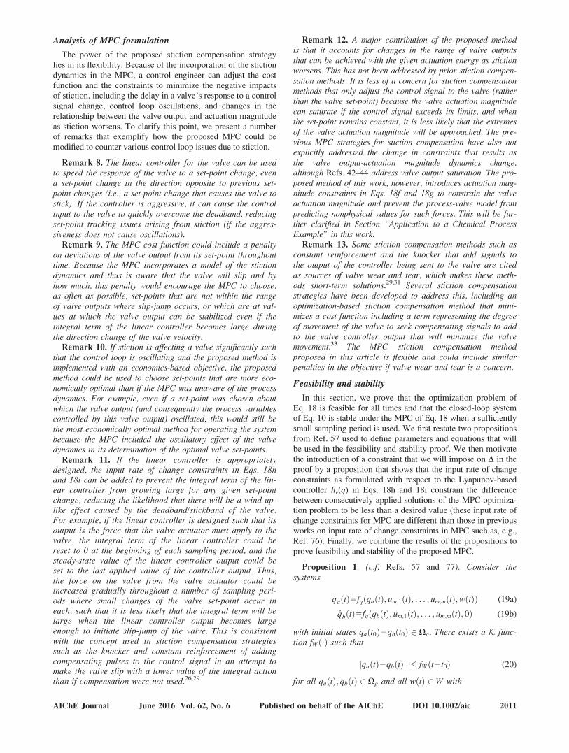
Figure 7. Open-loop values of ua and um for the nomi-nal valve.


0.5 td and record the value of ua at the end of every 0.5 td,

again using the Explicit Euler numerical integration method

with an integration time step of 1026 td (the Explicit Euler

numerical integration method with an integration time step of

1026 td was used for all simulations of the nominal valve in

this “Motivation for Actuation Magnitude Constraints” Sec-

tion). The resulting ua 2 P relationship can no longer be

described as one linear relation, but two that depend on

whether the pressure is being increased or decreased, and the

deadband at a velocity change is visible in Figure 6. In addi-

tion, it can be observed from the figure that because of the

effect of stiction on the ua 2 P relationship, there are certain

flow rates that can be achieved with a positive pressure for the

vendor valve that would require a negative pressure for the

nominal valve, which is physically not possible to achieve.

This is the first hint that to compensate for stiction, additional

constraints of the form of Eqs. 18f and 18g will need to be

added to the EMPC to prevent physically unrealizable set-

points from being requested.As shown in Figure 6, the linear relationship between um

and P developed in Eq. 45 is not sufficient to control a valve

subject to stiction. Further evidence of this comes from ramp-

ing the set-point um of the nominal open-loop valve up and

down between 0.1042 and 0.7042 in increments of 0.01 everysampling period of length D 5 0.2 td and determining the pres-

sure to apply to the valve from Eq. 45. The dynamic response

(i.e., not steady-state; this is the reason for the step-like quality

of the trajectories) of the valve output to these set-point

changes is shown in Figures 7 and 8. Figure 7 shows the insuf-

ficiency of Eq. 45 to determine the pressure value that should

be applied to the valve for a desired um because it shows that

for this sticky valve, ua does not effectively track um (the

ua 2 um plot in Figure 7 is not linear). This is further empha-

sized in Figure 8, which also shows the deadband when um

begins to change in the opposite direction to that in which it

was changing previously. This demonstrates that a different

relationship between um and P is needed to control the nomi-

nal valve than that provided by Eq. 45 to ensure good set-point

tracking.In the proposed method, the linear controller of Eqs. 43 and

44 is used to improve the set-point tracking performance of ua.

To demonstrate that this does indeed improve the set-point

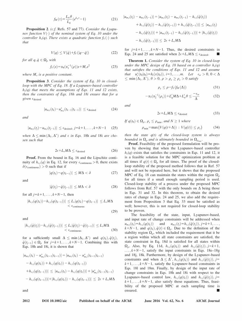
tracking, we ramp the set-point um to the nominal valve inclosed-loop with the linear controller in Eqs. 43 and 44, againramping it up and down between 0.1042 and 0.7042 in incre-ments of 0.01 every D 5 0.2 td. The dynamic response of thevalve is shown in Figures 9 and 10 which show that theua 2 um relationship is close to linear under the linear control-ler, and that ua is able to closely track um in time and is quicklyable to overcome the deadband caused by stiction. However,despite its benefit in providing good set-point tracking per-formance, the use of Eqs. 43 and 44 does not ensure that thevalue of P requested will not become negative. This is demon-strated in Figures 11 and 12, which plot the dynamic responseof the closed-loop valve to eight set-point changes(um50:35; 0:2; 0:35; 0:2; 0:3; 0:4; 0:5, and 0.6) each heldfor D 5 0.2 td when initialized from the fully open position(i.e., ua50:7042; Ps50 kg=m � t2d; xv50 m; vv50 m=td; zf 5

0 m initially). The results in Figure 11 again show that the PIcontrol law developed in Eqs. 43 and 44 helps the valve toeffectively track its set-points even when there is deadbandbecause the direction of the valve stem movement changes.However, the results of Figure 12 show that the good set-pointtracking can only be achieved when the pressure is able toadjust as necessary, including becoming negative, which isphysically impossible. From Figures 11 and 12, it can bededuced that if the pressure is saturated at 0 kg=m � t2d when alower pressure is requested, the valve output would not beable to reach all of the set-points in this simulation. This indi-cates that when the control law of Eqs. 43 and 44 is used, theconstraints of the EMPC need to ensure that the pressure doesnot become negative at the set-points it requests, because thecontrol law itself does not ensure this.

Remark 16. In this section, ramping of set-point changeswas used to demonstrate the good set-point trackingperformance of the PI controller in Eqs. 43 and 44. If theramping of the set-point changes is too rapid, however, the

Figure 8. Open-loop values of ua and um with time forthe nominal valve.

Figure 9. Closed-loop values of ua and um for the nom-inal valve under PI control.

The plot depicts that ua increases with increasing um and

decreases with decreasing um when the value of um is

changed by 0.01 every D. The arrow in the lower left

corner of the plot shows the direction in which the

increasing and decreasing steps in the plot are traversed.


closed-loop control valve under PI control may bedestabilized.

Remark 17. The constraint P � 0 kg=m � t2d was devel-oped for the EMPC in this section to ensure that the set-points calculated by the EMPC are physically realizable(i.e., that they do not require the pressure to become nega-tive for ua to meet um). Based on the plots presented in thissection, other methods for handling this scenario could beconsidered as well. For example, based on Figure 6,another method for preventing negative pressures for thisexample may be to decrease the range of allowable valuesof um as stiction worsens such that the allowable values ofum always correspond to positive pressures. However, itmay be difficult to determine what the new bound on um

should be without doing an offline test to generate data likethat in Figure 6, and the valve stiction may continue toworsen with time, meaning that new ranges for um mayneed to be determined throughout time. In addition,because the profit from EMPC may be improved by allow-ing operation over a larger region of state-space, it is notdesirable to choose extremely conservative bounds on um toavoid the calculation of set-points that would require nega-tive pressures because that may lower profit below thatwhich could be realized. Motivated by these considerations,for the EMPC in this example, we set the constraint of Eq.18g in our proposed MPC compensation strategy to be aconstraint that the actuator pressure must never becomenegative.

Remark 18. We note that the basic relationshipsbetween um, ua, and P presented in this section are well-known; for example, one can find plots similar to those inFigures 6–8 in Refs. 3–5. In addition, it is well-knownthat control of the valve position may help to improve theresponse of a valve in the presence of valve nonlinearities(e.g., Ref. 5 suggests a control law to bring the valveposition to its set-point in the presence of stiction, andRef. 33 states that valve positioners are often able toimprove a valve’s response if it exhibits deadband). Theresults in this section are novel, however, because theypresent the dynamic plots of the open and closed-loopvalve responses as an analysis tool useful for the designof an MPC with appropriate constraints for stiction com-

pensation and show how this analysis can be carried outusing plots of this type. Furthermore, this discussion isnot meant to be applicable only to this example, but tosuggest the type of thinking and analysis that may need togo into the design of the proposed MPC for otherprocesses.

Proposed MPC Formulation

In this section, we describe the performance of an EMPC

formulation meeting the form of our proposed MPC stiction

compensation strategy in Eq. 18 with the process-valve model

of Eqs. 36–44 and the constraint that P � 0 kg=m � t2d at all

times.The control objective is to maximize the yield of the prod-

uct ethylene oxide. The yield of ethylene oxide between the

initial and final times of the plant operation (t0 and tf) is

defined as

Figure 10. Closed-loop values of ua and um with timefor the nominal valve under PI control.

Figure 11. Closed-loop values of ua and um with timefor the nominal valve under PI control forseveral set-point changes.

Figure 12. Closed-loop values of the pressure withtime for the nominal valve under PI controlfor several set-point changes.


Yðtf Þ5

ðtf

t0

uaðsÞx3ðsÞx4ðsÞdsðtf

t0

uaðsÞCeds(46)

However, we assume that the volumetric flow rate of theinlet stream is bounded such that between t0 and tf, the follow-

ing integral holds

Ce

tf 2t0

ðtf

t0

uaðsÞds50:175 (47)

Combining Eqs. 46 and 47, the objective of the EMPC

becomes the maximization of the time integral of the stagecost LMPC, where LMPC is defined as follows

LMPC5uaðsÞx3ðsÞx4ðsÞ (48)

The input ua is physically bounded between the flow rates at

the maximum and minimum valve openings as follows

ua;min � ua � ua;max (49)

with ua,min 5 0 (valve fully closed) and ua,max 5 0.7042 (valve

fully open). The value of ua is computed using the actuatorlayer equations in Eqs. 37–44.

We assume that the only data available to aid in choosing

the allowable range of valve set-points um that the EMPC cal-culates is the vendor data in Figure 6. Thus, we assume that

the bounds developed for the EMPC include set-points that

can only be met with negative pressures by the nominalvalve, although they can be met with positive pressures by

the vendor valve. The set-points um are thus restricted as

follows

um;min � um � um;max (50)

with um,min 5 0.0704 and um,max 5 0.7042 (the minimum value

of um is greater than 0 because we assume that we want toavoid fully closing the valve for this process). Physically, the

pressure applied to the valve diaphragm cannot drop below0 kg=m � t2d .

For this example, the optimization variable ua does not havea large effect on the process economics, with the result that

the process yields under steady-state operation and underEMPC operation are approximately equal in the long term

when the valve has no stiction. Thus, we emphasize that the

choice to use EMPC for this example is primarily driven, aspreviously noted, by the ability of EMPC to promote time-

varying operation such that it computes set-points at the

bounds of what is physically possible to maximize the processprofit and thus effectively illustrates the advantages of includ-

ing the constraint on the actuation magnitude (pressure). Fur-thermore, the profitability of EMPC over steady-state

operation for a variety of processes has been well-documented

in the literature (see, e.g., Refs. 57 and 81), including for thepresent example when two actuators are used as in Ref. 45,

and is not the focus of this work. However, it is noted that the

process in the absence of stiction or valve dynamics has asteady-state yield of 6.63% over 468 td and a yield of 32.22%

over 2 td when initiated from ½x1I x2I x3I x4I�T5

½0:997 1:264 0:209 1:004�T . This shows that for the two oper-

ating periods considered in this study, the effect of the tran-

sient is very strong because the average steady-state yield ismuch larger over the 2 td considered in this study than it is

after a longer time period.

To achieve the above objectives while countering stiction,

we develop an EMPC, termed EMPC 2 A, that incorporates

actuator dynamics to aid in stiction compensation and maxi-

mizes the yield of ethylene oxide subject to the integral mate-

rial constraint and constraints on the allowable values of the

valve output, valve set-point, and actuator output to prevent

nonphysical situations. This EMPC solves the following opti-

mization problem

minumðtÞ2SðDÞ

2

ðtk1Nk

tk

~uaðsÞ~x3ðsÞ~x4ðsÞ ds (51a)

s:t: _~qðtÞ5fqð~qðtÞ; umðtÞÞ (51b)

~qðtkÞ5qðtkÞ (51c)

0 � ~uaðtÞ � 0:7042; 8 t 2 ½tk; tk1N � (51d)

0:0704 � umðtÞ � 0:7042; 8 t 2 ½tk; tk1NÞ (51e)

~PðtÞ � 0; 8 t 2 ½tk; tk1N � (51f)ðtk1Nk

tk

~uaðsÞds1

ðtk

ðj21Þtpu�aðsÞds5

0:175tpCe

(51g)

where the cost function in Eq. 51a represents the total yield of

ethylene oxide throughout the prediction horizon when the

material constraint is met, and Eq. 51g is the method for imple-

menting the integral material constraint by constraining the

value of ua to meet the material constraint in each operating

period. Equation 51g states that the time-average value of the

sum of the predicted valve outputs ~ua plus the previously

applied valve outputs u�a must be no greater than 0:175Ce

over the

jth operating period (j51; 2; . . .). A shrinking prediction hori-

zon is used, such that the prediction horizon Nk 5 5 at the

beginning of an operating period of length tp 5 1 td (D 5 0.2 td)

but is decremented by 1 at each subsequent sampling time in

the operating period. The use of this shrinking horizon allows

the integral material constraint of Eq. 47 to be implemented in

Eq. 51g. The state constraints in Eqs. 51d and 51f were

enforced every two integration steps. Because this process has

an asymptotically stable steady-state, the Lyapunov-based con-

straints of Eqs. 18l and 18m were not considered. The dynamic

equation in Eq. 51b was integrated within the EMPC using the

Explicit Euler numerical integration method with an integra-

tion step of hA51026 td. Centered finite difference approxima-

tions of derivatives required for the solution of the

optimization problem were obtained by perturbing the optimi-

zation variables by 1026.For comparison with EMPC 2 A, we also introduce an

EMPC that does not include the valve dynamics, which will

be referred to as EMPC 2 B, formulated as follows

minumðtÞ2SðDÞ

2

ðtk1Nk

tk

umðsÞ~x3ðsÞ~x4ðsÞ ds (52a)

s:t: _~xðtÞ5f ð~xðtÞ; umðtÞÞ (52b)


0:0704 � umðtÞ � 0:7042; 8 t 2 ½tk; tk1NÞ (52d)ðtk1Nk

tk

umðsÞds1

ðtk

ðj21Þtpu�mðsÞds5

0:175tpCe

(52e)

where the notation in Eq. 52b signifies that ua in Eqs. 36a–36d

is replaced by um in the model used to predict the process

states within EMPC 2 B. Numerical integration of the

dynamic equation in Eq. 52b was performed using the Explicit


Euler method with an integration time step of hB51024 td. Cen-tered finite difference approximations of derivatives required forthe solution of the optimization problem were obtained by per-turbing the optimization variables by 1024.

A third EMPC, EMPC 2 C, was also developed with theform of EMPC 2 B but with rate of change constraints added,for reasons that will be clarified below. EMPC 2 C solves thefollowing optimization problem

minumðtÞ2SðDÞ

2

ðtk1Nk

tk

umðsÞ~x3ðsÞ~x4ðsÞ ds (53a)

s:t: _~xðtÞ5f ð~xðtÞ; umðtÞÞ (53b)


0:0704 � umðtÞ � 0:7042; 8 t 2 ½tk; tk1NÞ (53d)ðtk1Nk

tk

umðsÞds1

ðtk

ðj21Þtpu�mðsÞds5

0:175tp

Ce(53e)

jumðtkÞ2u�mðtk21jtk21Þj � c (53f)

jumðtjÞ2umðtj21Þj � c; j5k11; . . . ; k1Nk21 (53g)

where c in Eqs. 53f and 53g is a constant that defines thechange in um that will be accepted between sampling periods.In the following simulations, c 5 0.1. Equation 53b wasnumerically integrated using the Explicit Euler numerical inte-gration method with an integration step size of hC51024 td.Centered finite difference approximations of derivativesrequired for the solution of the optimization problem wereobtained by perturbing the optimization variables by 1024.

Outside of EMPC 2 A, EMPC 2 B, and EMPC 2 C, theactual process was simulated using Eqs. 36–44 with anExplicit Euler integration step size of h51026 td, with thepressure saturated at 0 kg=m � t2d if a lower pressure wasrequested (ua would have been saturated at ua,min or ua,max ifthose values were exceeded, but neither of these extremeswere violated in these simulations). All three EMPC’s usedtp51 td; D50:2 td, and simulated the results for two operat-ing periods. They were initiated from the point qI5½0:9971:264 0:209 1:004 0:051 2:00031026 1:42631025 0�T , wh-ere the process states are dimensionless and the states of theactuator layer have SI units except for a dimensionless time

unit as in Table 1, and the initial value of the steady-statepressure is Ps;I563; 713 kg=m � t2d. All optimizations wereperformed using the open-source nonlinear interior pointoptimization solver Ipopt82 and were coded in the C11 pro-gramming language. The Ipopt convergence tolerance foroptimization termination was set to 10210 for EMPC 2 A,and to 1028 for EMPC 2 B and EMPC 2 C. Simulationswere carried out on a 2.40 GHz Intel Core 2 Quad CPUQ6600 on a 64-bit Windows 7 Professional operating systemwith 4.00 GB of RAM.

Figures 13 and 14 show the values of ua, um, and P for thevalve with time when the system of Eqs. 36–44 is controlledby EMPC 2 A and EMPC 2 B. These figures show that theinclusion of valve dynamics and actuation magnitude con-straints in EMPC causes EMPC 2 A to calculate lower set-points than EMPC 2 B, which allows the valve output to trackthe EMPC-requested set-points throughout the two operatingperiods, even when the pressure drops, because EMPC 2 A isaware of the limitations of the pneumatic actuation and thuscalculates set-points that the valve output can reach (it is notedthat there are two small set-point changes in Figure 13 that ua

for EMPC 2 A does not track; the reason for this will beexplained further below, but the overall trend that ua tracks um

well under EMPC 2 A can be deduced from Figure 13). Fig-ures 13 and 14 show that when the actuator dynamics are notincluded in EMPC and stiction develops with time such thatthe pressure-flow rate relationship is altered, the valve outputis not able to track the EMPC 2 B set-points becauseEMPC 2 B calculates set-points for which the pressure wouldneed to drop to negative values to allow the valve to moveenough to reach them (because this is physically impossible,the pressure under EMPC 2 B saturates at its minimum valueof 0 kg=m � t2d for four sampling periods, although the pressureunder EMPC 2 A does not because the set-points calculatedby EMPC 2 A are reachable). The inability of the valve toreach the set-points calculated by EMPC 2 B causes theEMPC 2 B optimization problem to become infeasible in thelast two sampling periods of each operating period and causesEMPC 2 B to be unable to meet the integral constraint (it can-not use all available material; the value of the integral con-straint in Eq. 47 calculated for each operating period (i.e.,

Figure 13. Valve output set-points um (solid trajectories) and actual valve outputs ua (dashed trajectories) through-out two operating periods for EMPC 2 A, EMPC 2 B, and EMPC 2 C.


between ðj21Þtp and jtp, j 5 1, 2, instead of between t0 and tf) is

approximately 0.133, which is 24% less than the required value

of 0.175). The yield of EMPC 2 A throughout two operatingperiods according to Eq. 46 is 32.4%, while that of EMPC 2 Baccording to Eq. 46 is 35.1%. This at first appears to suggest

that EMPC 2 B out-performs EMPC 2 A economically; how-

ever, because EMPC 2 B did not meet a hard constraint of the

process, the yield that it achieved without meeting this con-

straint cannot be compared with the yield of a process that did

meet the constraint. Thus, no further discussion of yields underthe various EMPC’s will be pursued, and the discussion will

focus on the degree to which the various formulations ensure

that the process constraints are satisfied. In contrast to

EMPC 2 B, EMPC 2 A is feasible in both operating periods.Despite the advantages of using EMPC 2 A rather than

EMPC 2 B to ensure that all process constraints are met, the

computational burden of EMPC 2 A due to the enforcement ofthe constraints on the pressure and on ua at every other inte-

gration step hA51026 td within the EMPC is much larger than

that for EMPC 2 B. In an actual plant, this computation time

increase could prohibit the use of EMPC 2 A if the process

has fast dynamics such that a short sampling time is required

for effective control. However, the input rate of change con-

straints discussed in this article for the design of an MPCincorporating nonlinear valve dynamics may be considered for

use in EMPC 2 B to minimize the large jumps in um that cause

EMPC 2 B to be unable to meet the material constraint at the

end of the operating periods but without adding much compu-

tation time. Thus, we demonstrate the use of input rate of

change constraints and how they affect the trajectories of um,ua, and P using EMPC 2 C. Figures 13 and 14 show these tra-

jectories and show that the addition of the input rate of change

constraints to EMPC 2 B to form EMPC 2 C significantly

improves the set-point tracking performance compared to

EMPC 2 B. In contrast to EMPC 2 B, for which four of the

set-points were not reachable and caused significant offset,

there is only one set-point calculated by EMPC 2 C in Figure13 for which offset is observed, and the offset is much smaller

than those for EMPC 2 B. In addition, the pressure in Figure

14 only saturates at its minimum value for one sampling

period under EMPC 2 C, instead of the four during which it

saturates under EMPC 2 B. Although EMPC 2 C is infeasible

for three sampling periods (the last two sampling periods of

the first operating period and the last sampling period of the

second operating period) and the integral constraint is not met

at the end of either operating period, the degree to which the

integral constraint is violated is significantly less than under

EMPC 2 B (the integral constraint is 0.171 at the end of the

first operating period and 0.172 at the end of the second under

EMPC 2 C, such that in each operating period, it is only about

2% less than the required value of 0.175). In addition, the

computation time of EMPC 2 C is, as for EMPC 2 B, much

lower than that for EMPC 2 A owing to the use of a lower-

order model than EMPC 2 A. The rate of change constraints

were added to EMPC 2 C in an ad hoc fashion and are not

guaranteed to reduce the negative effects of stiction on the

controller performance, but the positive impact that they had

on the process performance does indicate the breadth of con-

straints that could be considered to combat the effects of stic-

tion with both the proposed MPC and also with MPC’s for

processes that cannot fully incorporate the proposed method

due to computation time constraints.Figures 15 and 16 show the closed-loop process and actua-

tor layer states under EMPC 2 A, EMPC 2 B, and EMPC 2 C.

Figure 15 shows that the process state trajectories are not dras-

tically affected by the differences between the trajectories of

ua under the three EMPC’s, which contributes to the fact that

the focus of this example is not on the profitability of the pro-

posed EMPC compared to the other methods, but rather on its

ability to meet the constraints of the process when the valve is

affected by stiction. The plot of the controller state f in Figure

16 shows the manner in which the integral term of the control-

ler is affected by the different EMPC formulations. In

EMPC 2 B, the integral term becomes large in the sampling

periods in which the EMPC cannot reach its set-points. This

plot also shows the benefits of resetting the value of f to zero

at each set-point change so that, for example, the value of ffor EMPC 2 B at the beginning of the second operating period

is not wound up from the integration of this state at the end of

Figure 14. Actuator pressure applied to valve stemthroughout two operating periods forEMPC 2 A (solid trajectory), EMPC 2 B(dashed trajectory), and EMPC 2 C (dottedtrajectory).

Figure 15. Closed-loop process states x1, x2, x3, and x4

throughout two operating periods underEMPC 2 A (solid trajectories), EMPC 2 B(dashed trajectories), and EMPC 2 C (dottedtrajectories).


the first operating period. In addition, the plot shows that theinclusion of the actuator dynamics and constraints on the pres-sure in EMPC 2 A and rate of change constraints inEMPC 2 C prevent the integral term from becoming largebecause they ensure that the set-points can be met or (in thecase of EMPC 2 C) reached closely enough so that the integralterm does not reach large values. In addition, the increase in fat a direction change of the velocity to allow the pressure toovercome the deadband is visible in this plot as well.

The trajectories in Figures 13, 14, and 16 show the relation-ships between the physical states xv and vv of the valve and thevalve output and pressure applied to the valve for the processunder EMPC 2 A, EMPC 2 B, and EMPC 2 C. Because thevalue of ua is an explicit function of xv, changes in ua occurwhen xv changes. A comparison of the trajectories of xv and ua

with the values of P for EMPC 2 A shows the deadband wherethe pressure is increasing but the values of xv and ua do notchange much because the error (and thus f) is not large enoughto cause much stem movement for the small set-point changestoward the end of the first and second operating periods of theEMPC. The set-point changes in EMPC 2 B and EMPC 2 Care all significant enough that the deadband is overcomewithin a sampling period. The velocity vv for all three EMPC’sis nonzero when xv and thus ua are changing, but is zero whenua reaches um and the friction force balances the pressure andspring forces on the valve.

The trajectories of zf in Figure 16 show that when deadbandis encountered, the state zf is driven through zero. This is con-sistent with the physical visualization of zf suggested by theauthors of the LuGre model,16 which related it to the averagedeflection of theoretical bristles on two contacting surfaces,whose bending caused friction. It would be expected that bris-tles would be deflected from an equilibrium (zero) locationcorresponding to the starting position of the valve when thestem position first begins to move in a given direction. In addi-tion, it is necessary for continuity of the friction force inEq. 39 that the value of zf approach this zero value in adynamic fashion, rather than abruptly. The passing of zf

through zero at a change in the direction of set-point changes

allows the friction force of Eq. 39 to change direction so that it

continues to be in the direction opposite the applied force.We now address the fact that EMPC 2 A calculated set-

points that are not reachable (see Figure 13) although it could

predict the dynamics of the valve with respect to the set-point

changes. Stiction is often noticeable when pressure is applied

to a valve, but the valve stem does not move because the

opposing friction force is significant. This phenomenon is

exhibited during the two set-point changes for EMPC 2 A that

the valve output does not track. Due to the small set-point

reversals in um requested by EMPC 2 A at the end of the first

and second operating periods, the value of the pressure applied

to the valve according to Eqs. 43 and 44 does not change

quickly as the error between um and ua (and thus f) is low.

However, although the valve is considered to be stuck at this

time, as the pressure changes, the dynamics in Eqs. 37–41

cause the stem position and velocity (in addition to zf) to con-

tinue to change, although slowly. It is because of this effect

that EMPC 2 A calculates set-points that it cannot reach; it

does so to manipulate the numerical results such that the valve

stem and thus output would move just enough in the sampling

periods in which unreachable set-points are calculated to allow

all constraints to be met, including the integral constraint.

While this suggests that the results are dependent on the fric-

tion model used, it also shows that including the friction model

within the EMPC allows the EMPC to make smart set-point

choices that are not necessarily intuitive.To demonstrate the robustness of the proposed approach to

disturbances and plant-model mismatch, the process of Eqs.

36–44 was controlled by EMPC 2 A and was simulated with

different levels of bounded Gaussian white noise in the pro-

cess and actuator states, and the closed-loop stability of the

process under EMPC 2 A was found to be robust with respect

to the different noise levels. In addition, when the process was

simulated with noise in the process states with standard

deviation rw5½0:1 300 60 0:4 0 0 0 0�T and bound h5

½0:3 900 180 1:2 0 0 0 0�T (this standard deviation and bound on

the noise were chosen because they provided a meaningful

perturbation to the process states when added to the right-hand

side of Eqs. 36a–36d), the integral material constraint was met

in both operating periods.

Conclusions

In this work, we showed that MPC can be used to compen-

sate for the effects of stiction by including detailed valve

dynamics for sticky valves in addition to constraints on the

rate of change of inputs and the actuation magnitude.

Although the focus of the proposed method was on stiction

compensation, it could be considered for ameliorating the neg-

ative effects of other nonlinear valve behavior, such as back-

lash resulting in deadband. We defined the process-valve

model in general terms so that the proposed approach could be

adapted to a variety of valve types. The flexibility of the

MPC-based stiction compensation strategy, which allows it to

incorporate a variety of cost functions or constraints to reduce

tracking offset or oscillations in control loops, was discussed.

In addition, closed-loop stability and feasibility of the MPC

optimization problem including Lyapunov-based stability con-

straints were proven for a sufficiently small sampling period.

Using a chemical process example, we showed how con-

straints can be developed for the MPC for stiction compensa-

tion and demonstrated that this MPC can result in better valve

Figure 16. Closed-loop actuator layer states xv, vv, z,and f throughout two operating periodsunder EMPC 2 A (solid trajectories),EMPC 2 B (dashed trajectories), andEMPC 2 C (dotted trajectories).


layer set-point tracking and constraint satisfaction than an

MPC that does not account for stiction.

Acknowledgment

Financial support from the National Science Foundation

and the Department of Energy is gratefully acknowledged.

Literature Cited

1. Desborough L, Miller R. Increasing customer value of industrialcontrol performance monitoring-Honeywell’s experience. In AIChESymposium Series. New York: American Institute of Chemical Engi-neers, 2002:172–192.

2. Nallasivam U, Babji S, Rengaswamy R. Stiction identification innonlinear process control loops. Comput Chem Eng 2010;34:1890–1898.

3. Choudhury MAAS, Thornhill NF, Shah SL. Modelling valve stiction.Control Eng Pract 2005;13:641–658.

4. Garcia C. Comparison of friction models applied to a control valve.Control Eng Pract. 2008;16:1231–1243.

5. Kayihan A, Doyle FJ III. Friction compensation for a process controlvalve. Control Eng Pract. 2000;8:799–812.

6. Choudhury MAAS. Plantwide oscillations diagnosis-current state andfuture directions. Asia-Pac J Chem Eng. 2011;6:484–496.

7. Choudhury MAAS, Jain M, Shah SL. Stiction-definition, modelling,detection and quantification. J Process Control. 2008;18:232–243.

8. Br�asio ASR, Romanenko A, Fernandes NCP. Modeling, detectionand quantification, and compensation of stiction in control loops:The state of the art. Ind Eng Chem Res. 2014;53:15020–15040.

9. Armstrong-H�elouvry B, Dupont P, Canudas de Wit C. A survey ofmodels, analysis tools and compensation methods for the control ofmachines with friction. Automatica. 1994;30:1083–1138.

10. Swevers J, Al-Bender F, Ganseman CG, Prajogo T. An integratedfriction model structure with improved presliding behavior for accu-rate friction compensation. IEEE Trans Autom Control. 2000;45:675–686.

11. Al-Bender F, Lampaert V, Swevers J. A novel generic model atasperity level for dry friction force dynamics. Tribol Lett. 2004;16:81–93.

12. Wang J, Zhang Q. Detection of asymmetric control valve stictionfrom oscillatory data using an extended Hammerstein system identi-fication method. J Process Control. 2014;24:1–12.

13. Olsson H, Astr€om KJ, Canudas de Wit C, G€afvert M, Lischinsky P.Friction models and friction compensation. Eur J Control. 1998;4:176–195.

14. Dahl PR. A Solid Friction Model. Technical Report TOR-0158(3107-18)21. El Segundo, CA: Aerospace Corporation, 1968.

15. Olsson H. Control Systems with Friction. PhD Thesis. Lund Instituteof Technology, 1996.

16. Canudas de Wit C, Olsson H, Astr€om KJ, Lischinsky P. A newmodel for control of systems with friction. IEEE Trans Autom Con-trol. 1995;40:419–425.

17. Lampaert V, Swevers J, Al-Bender F. Modification of the Leuvenintegrated friction model structure. IEEE Trans Autom Control.2002;47:683–687.

18. Dupont P, Armstrong B, Hayward V. Elasto-plastic friction model:contact compliance and stiction. In Proceedings of the AmericanControl Conference. Chicago, IL, 2000:1072–1077.

19. Lampaert V, Al-Bender F, Swevers J. A generalized Maxwell-Slipfriction model appropriate for control purposes. In Proceedings ofthe International Conference on Physics and Control. St. Petersburg,Russia, 2003:1170–1177.

20. Stenman A, Gustafsson F, Forsman K. A segmentation-based methodfor detection of stiction in control valves. Int J Adapt Control SignalProcess. 2003;17:625–634.

21. Kano M, Maruta H, Kugemoto H, Shimizu K. Practical model anddetection algorithm for valve stiction. In Proceedings of the IFACSymposium on Dynamics and Control of Process Systems. Cam-bridge, MA, 2004:859–864.

22. He QP, Wang J, Pottmann M, Qin SJ. A curve fitting method fordetecting valve stiction in oscillating control loops. Ind Eng ChemRes. 2007;46:4549–4560.

23. Feemster M, Vedagarbha P, Dawson DM, Haste D. Adaptive controltechniques for friction compensation. In Proceedings of the Ameri-can Control Conference. Philadelphia, PA, 1998:1488–1492.

24. Friedland B, Park Y-J. On adaptive friction compensation. IEEETrans Autom Control. 1992;37:1609–1612.

25. Huang SN, Tan KK, Lee TH. Adaptive friction compensation usingneural network approximations. IEEE Trans Syst Man Cybern CAppl Rev. 2000;30:551–557.

26. H€agglund T. A friction compensator for pneumatic control valves.J Process Control. 2002;12:897–904.

27. Sivagamasundari S, Sivakumar D. A new methodology to compen-sate stiction in pneumatic control valves. Int J Soft Comput Eng.2013;2:480–484.

28. Coughanowr DR, LeBlanc SE. Process Systems Analysis and Con-trol, 3rd ed. Boston, MA: McGraw-Hill, 2009.

29. Ivan LZX, Lakshminarayanan S. A new unified approach to valvestiction quantification and compensation. Ind Eng Chem Res. 2009;48:3474–3483.

30. Jamaludin Z, Van Brussel H, Swevers J. Design of a disturbanceobserver and model-based friction feedforward to compensate quad-rant glitches. In: Ulbrich H, Ginzinger L, editors. Motion and Vibra-tion Control. The Netherlands: Springer, 2009:143–153.

31. Cuadros MAdSL, Munaro CJ, Munareto S. Novel model-freeapproach for stiction compensation in control valves. Ind Eng ChemRes. 2012;51:8465–8476.

32. Srinivasan R, Rengaswamy R. Stiction compensation in process con-trol loops: a framework for integrating stiction measure and compen-sation. Ind Eng Chem Res. 2005;44:9164–9174.

33. Srinivasan R, Rengaswamy R. Approaches for efficient stiction com-pensation in process control valves. Comput Chem Eng. 2008;32:218–229.

34. Cuadros MAdSL, Munaro CJ, Munareto S. Improved stiction com-pensation in pneumatic control valves. Comput Chem Eng. 2012;38:106–114.

35. Wang J. Closed-loop compensation method for oscillations causedby control valve stiction. Ind Eng Chem Res. 2013;52:13006–13019.

36. Gerry J, Ruel M. How to measure and combat valve stiction online.In Proceedings of the ISA International Fall Conference. Houston,TX, 2001.

37. Li C, Choudhury MAAS, Huang B, Qian F. Frequency analysis andcompensation of valve stiction in cascade control loops. J ProcessControl. 2014;24:1747–1760.

38. Ale Mohammad M, Huang B. Compensation of control valve stictionthrough controller tuning. J Process Control. 2012;22:1800–1819.

39. Cheng C-C, Chen C-Y, Chiu G T-C. Predictive control withenhanced robustness for precision positioning in frictional environ-ment. IEEE/ASME Trans Mechatronics. 2002;7:385–392.

40. Hampson SP. Nonlinear Model Predictive Control of a HydraulicActuator: Theory and Implementation. PhD Thesis. University ofCanterbury, 1995.

41. Su SW, Nguyen H, Jarman R, Zhu J, Lowe D, McLean P, Huang S,Nguyen NT, Nicholson R, Weng K. Model predictive control of agantry crane with input nonlinearity compensation. In Proceedingsof the World Academy of Science, Engineering and Technology.Penang, Malaysia, 2009: 312–316.

42. Zabiri H, Samyudia Y. A hybrid formulation and design of modelpredictive control for systems under actuator saturation and backlash.J Process Control. 2006;16:693–709.

43. Zabiri H, Samyudia Y. MIQP-based MPC in the presence of controlvalve stiction. Chem Prod Process Model. 2009;4:85–97.

44. del Carmen Rodr�ıguez Li~n�an M, Heath WP. MPC for plants subjectto saturation and deadzone, backlash or stiction. In Proceedings ofthe 4th IFAC Nonlinear Model Predictive Control Conference. Noor-wijkerhout, The Netherlands, 2012:418–423.

45. Durand H, Ellis M, Christofides PD. Integrated design of controlactuator layer and economic model predictive control for nonlinearprocesses. Ind Eng Chem Res. 2014;53:20000–20012.

46. Belimo AirControls (USA), Inc. Electronic Valve ApplicationsGuide. DOC.V4.2-03.99-7.5M. Available at: http://www.belimo.us/americas/resources.html. Accessed on October 20, 2015.

47. Bishop T, Chapeaux M, Jaffer L, Nair K, Patel S. Ease control valveselection. Chem Eng Prog. 2002:52–56.

48. Liptak BG, Boyes WH. Applying control valves. In: Boyes W, edi-tor. Instrumentation Reference Book, 4th ed. Boston, MA: Butter-worth-Heinemann, 2010:631–636.

49. Darby ML, Nikolaou M, Jones J, Nicholson D. RTO: an overview andassessment of current practice. J Process Control. 2011;21:874–884.

50. Christofides PD, El-Farra NH. Control of Nonlinear and Hybrid Pro-cess Systems: Designs for Uncertainty, Constraints and Time-Delays.Berlin, Germany: Springer-Verlag, 2005.


51. Khalil HK. Nonlinear Systems, 3rd ed. Upper Saddle River, NJ:Prentice Hall, 2002.

52. El-Farra NH, Christofides PD. Bounded robust control of constrainedmultivariable nonlinear processes. Chem Eng Sci. 2003;58:3025–3047.

53. Lin Y, Sontag ED. A universal formula for stabilization withbounded controls. Syst Control Lett. 1991;16:393–397.

54. Mhaskar P, El-Farra NH, Christofides PD. Stabilization of nonlinearsystems with state and control constraints using Lyapunov-based pre-dictive control. Syst Control Lett. 2006;55:650–659.

55. Mu~noz de la Pe~na D, Christofides PD. Lyapunov-based model pre-dictive control of nonlinear systems subject to data losses. IEEETrans Autom Control. 2008;53:2076–2089.

56. Qin SJ, Badgwell TA. A survey of industrial model predictive con-trol technology. Control Eng Pract. 2003;11:733–764.

57. Heidarinejad M, Liu J, Christofides PD. Economic model predictivecontrol of nonlinear process systems using Lyapunov techniques.AIChE J. 2012;58:855–870.

58. Ellis M, Durand H, Christofides PD. A tutorial review of economic modelpredictive control methods. J Process Control. 2014;24:1156–1178.

59. Rawlings JB, Angeli D, Bates CN. Fundamentals of economic modelpredictive control. In Proceedings of the 51st IEEE Conference onDecision and Control. Maui, HI, 2012:3851–3861.

60. Christofides PD, Liu J, Mu~noz de la Pe~na D. Networked and Distrib-uted Predictive Control: Methods and Nonlinear Process NetworkApplications. Advances in Industrial Control Series. London, Eng-land: Springer-Verlag, 2011.

61. Amrit R, Rawlings JB, Angeli D. Economic optimization usingmodel predictive control with a terminal cost. Annu Rev Control.2011;35:178–186.

62. Mayne DQ. Control of constrained dynamic systems. Eur J Control.2001;7:87–99.

63. Diehl M, Amrit R, Rawlings JB. A Lyapunov function for economicoptimizing model predictive control. IEEE Trans Autom Control.2011;56:703–707.

64. Fagiano L, Teel AR. Generalized terminal state constraint for modelpredictive control. Automatica. 2013;49:2622–2631.

65. Huang R, Biegler LT, Harinath E. Robust stability of economicallyoriented infinite horizon NMPC that include cyclic processes.J Process Control. 2012;22:51–59.

66. Mayne DQ, Rawlings JB, Rao CV, Scokaert POM. Constrainedmodel predictive control: stability and optimality. Automatica. 2000;36:789–814.

67. Ellis M, Durand H, Christofides PD. Elucidation of the role of con-straints in economic model predictive control. Annu Rev Control. Inpress.

68. Srinivasan R, Rengaswamy R, Miller R. Control loop performanceassessment. 1. A qualitative approach for stiction diagnosis. Ind EngChem Res. 2005;44:6708–6718.

69. Horch A. Condition Monitoring of Control Loops. PhD Thesis.Royal Institute of Technology, 2000.

70. Anderson KL, Blankenship GL, Lebow LG. A rule-based adaptivePID controller. In Proceedings of the 27th IEEE Conference onDecision and Control. Austin, TX, 1988:564–569.

71. Leosirikul A, Chilin D, Liu J, Davis JF, Christofides PD. Monitoringand retuning of low-level PID control loops. Chem Eng Sci. 2012;69:287–295.

72. Veronesi M, Visioli A. Performance assessment and retuning ofPID controllers for integral processes. J Process Control. 2010;20:261–269.

73. Choudhury MAAS, Shah SL, Thornhill NF, Shook DS. Automaticdetection and quantification of stiction in control valves. ControlEng Pract. 2006;14:1395–1412.

74. Lee KH, Ren Z, Huang B. Novel closed-loop stiction detection andquantification method via system identification. In Proceedings ofthe International Symposium on Advanced Control of IndustrialProcesses. Jasper, Canada, 2008.

75. Lao L, Ellis M, Christofides PD. Smart manufacturing: handling pre-ventive actuator maintenance and economics using model predictivecontrol. AIChE J. 2014;60:2179–2196.

76. Mhaskar P, Kennedy AB. Robust model predictive control of nonlin-ear process systems: handling rate constraints. Chem Eng Sci. 2008;63:366–375.

77. Mhaskar P, Liu J, Christofides PD. Fault-Tolerant Process Control:Methods and Applications. London, England: Springer-Verlag, 2013.

78. €Ozg€ulsen F, Adomaitis RA, Cinar A. A numerical method for deter-mining optimal parameter values in forced periodic operation. ChemEng Sci. 1992;47:605–613.

79. Alfani F, Carberry JJ. An exploratory kinetic study of ethylene oxi-dation over an unmoderated supported silver catalyst. Chim Ind.1970;52:1192–1196.

80. Romanenko A, Santos LO, Afonso PAFNA. Application of agenttechnology concepts to the design of a fault-tolerant control system.Control Eng Pract. 2007;15:459–469.

81. Ellis M, Christofides PD. Real-time economic model predictive con-trol of nonlinear process systems. AIChE J. 2015;61:555–571.

82. W€achter A, Biegler LT. On the implementation of an interior-pointfilter line-search algorithm for large-scale nonlinear programming.Math Program. 2006;106:25–57.

Manuscript received Oct. 27, 2015, and revision received Jan. 8, 2016.


Documents

Actuator Stiction Compensation via Model Predictive