Journal of Power and Energy Engineering, 2016, 4, 9-25 Published Online August 2016 in SciRes. http://www.scirp.org/journal/jpee http://dx.doi.org/10.4236/jpee.2016.48002

How to cite this paper: Bhutka, J., Gajjar, J. and Harinarayana, T. (2016) Modelling of Solar Thermal Power Plant Using Parabolic Trough Collector. Journal of Power and Energy Engineering, 4, 9-25. http://dx.doi.org/10.4236/jpee.2016.48002

Modelling of Solar Thermal Power Plant Using Parabolic Trough Collector Jignasha Bhutka*, Jaymin Gajjar, T. Harinarayana Gujarat Energy Research & Management Institute (GERMI), Gandhinagar, India

Received 17 June 2016; accepted 30 July 2016; published 2 August 2016

Copyright © 2016 by authors and Scientific Research Publishing Inc. This work is licensed under the Creative Commons Attribution International License (CC BY). http://creativecommons.org/licenses/by/4.0/

Abstract The target of the National Solar Mission is to build up India as a worldwide pioneer in solar energy generation. Solar power can be transmitted through grid either from solar photovoltaic or solar thermal technology. As compared to solar photovoltaic, solar thermal installations are less studied, especially regarding energy estimation and performance analysis. For estimating the potential of CSP plants, it is planned to simulate a power plant. We have marginally modified the design of 1 MW operational power plant installed at Gurgaon using Parabolic Trough Collector (PTC) tech-nology. The results are compared with the expected output of Gurgaon power plant and also 50 MW power plant at Rajasthan. Our results have closely matched with a small deviation of 3.1% and 3.6% for Gurgaon and Rajasthan plants, respectively. Our developed model is also validated with 18 different solar power plants in different parts of the world by slightly modifying the pa-rameters according to the plant capacity without changing major changes to the plant design. Dif-ference between our results and the expected energy generation varied from 0.4% to 13.7% with an average deviation of 6.8%. As our results show less than 10% deviation as compared to the ac-tual generation, an attempt has been made here to estimate the potential for the entire nation. For this modelling has been carried out for every grid station of 0.25˚ × 0.25˚ interval in India. Our re-sults show that annual solar thermal power plant of 1 MWe capacity potential varies from 900 to 2700 MWh. We have also compared our results with previous studies and discussed.

Keywords Parabolic Trough, Solar Thermal Power, TRNSYS, Simulation, India

1. Introduction It is well known that Government of India has put up a major target of 100 GW of electric power from solar in-

*Corresponding author.

J. Bhutka et al.

10

stallations by the near 2022. As of now we have 7.57 GW as installed capacity [1] [2]. It is well known that, so-lar energy is of two types-solar photovoltaic and solar thermal. For generating power from solar thermal power system, the following four technologies are presently being used: 1. Parabolic Trough collector (PTC); 2. Linear Fresnel Reflector (LFR); 3. Dish Sterling; 4. Solar Power Tower [3]. Among these technologies, parabolic trough collector is more popular and being used at many locations worldwide. Accordingly, large Concentrated Solar Power (CSP) plants are of PTC technology [4]. Global installed CSP had hiked from 355 MW in 2005 to more than 4700 MW in 2015 and it was predicted that the market would increase further in the years to come [5].

Lippke [6] has compared the results of his model with the results of real plant conditions for winter and sum-mer seasons to test the accuracy. It is concluded that the model is inadequate to fully match with actual solar field conditions. Valan and Sornakumar [7] have used a computer simulation program to model the parabolic trough collector with hot water generation system with a well-mixed type storage tank. From the verification of the model with actual generation 6% deviation is obtained. Yadav et al. [8] have examined, analysed and tested the parabolic trough collector with different type of reflectors. They identified aluminium sheet as cost effective material to use as reflector. In Spain, there are three power plants namely Andasol 1, Andasol 2 and Andasol 3 that are being operated using parabolic trough collector technology with a capacity of 50 MW each. The annual peak efficiency of each plant is 28% and average efficiency is 15%. The plants are operating with thermal stor-age of 7.5 hours using molten salt [9]. Price et al. [10] have validated their FLAGSOL model based on Parabolic Trough Collector. The projected performance and actual performance of a 30 MW Solar Energy Generation System (SEGS) plant over a full year of operation is 6%. This is developed by KJC Operating Company at Kramer Junction, California. Purohit [11] et al. evaluate the CSP potential of 2000 GW in north-western India in the available waste land and solar radiation assessment with viability of different technologies with 50 MW ca-pacity of PTC based plant. Similar to our simulation study, earlier workers have also computed for different plants. However, our study is more general and broad based.

Jones et al. [12] created a 30 MWe SEGS VI parabolic trough collector base power plant model in TRNSYS to evaluate the behaviour of solar field and power cycle with 10% difference between model and plant data. The thermodynamic properties data of HTF and steam have reasonably good accuracy. Kolb [13] evaluates the per-formance of 1 MWe Sugurao solar trough power plant with and without thermal storage using TRNSYS soft-ware. He obtaines plant efficiency of 7.8% with 23% capacity factor. It closely matches the actual data of the plant. He observed a peak operating temperature of HTF in Organic Rankine Cycle as 300˚C. Abdelkader et al. [14] have studied technical performance of 30 MWe PTC base power plant in Algerian weather conditions. Us-ing TRNSYS software they got annual average efficiency of solar field and power plant is 40.9% and 12%, re-spectively with highest power generation of 32 MWe. Abdel et al. [15] developed a model of 30-MW SEGS-VI solar power plant in TRNSYS 17 to measure electric power generation potential of Makkah. The maximum power of 34 MWe is generated with maximum temperature of 375˚C. Reddy and Harinarayana [16] have esti-mated the solar thermal energy potential in Indiawith1˚ interval in a grid manner. The energy generation ranges from 600 MWh to 2600 MWh annually for parabolic trough technology of 1 MWe capacity plant. The following are the input parameters in their TRNSYS model (Table 1).

The research work on CSP design, installation and monitoring would definitely enhance the growth of solar thermal sector. Because of technical, market and environmental challenges, CSP has not taken off in India

Table 1. Input Parameters used in simulation [16].

No Equipment Input and initial parameters

1. PTC field For example, length of Solar Collector Assembly (SCA): 120 m, row spacing = 12.5 m, inlet temperature = 227˚C, DNI = 2160 KJ/hr∙m2, Ambient Temperature = 23˚C, loss coefficient parameter: A = 73.6, B = 0.0042, C = 7.40

2. Turbine Mechanical efficiency = 0.99

3. High temperature tank Volume = 20 m3, maximum level = 18 m3, minimum level = 5 m3, dry loss co-efficient: 4 KJ/hr∙m2∙K

4. Low temperature tank Volume = 20 m3, maximum level = 18 m3, minimum level = 5 m3, dry loss co-efficient: 4 KJ/hr∙m2∙K

5. Super heater Heat exchanger type: rankine cycle, input temperature = 390˚C

6. Steam generator Heat exchanger type: rankine cycle, input temperature = 260˚C

7. Preheater Heat exchanger type: rankine cycle, input temperature = 105˚C

J. Bhutka et al.

11

although there is good solar thermal potential. There is no software based model validated with multiple operat-ing parabolic trough power plants that can be useful to estimate the solar thermal potential for different locations.

In view of above, our study is planned to construct and develop a standard model using TRNSYS software for forecasting the energy generation of CSP plants. For this purpose, 1 MW Solar Thermal Power Plant near Gur-gaon, New Delhi is considered and the plant is modelled with slight modification in the plant design. The simu-lated model is compared with the existing plants around the world.

TRNSYS is an extremely adaptable graphical software, based on programming environment used to simulate the behaviour of transient systems [17]. The main purpose of this software is to assess the performance of ther-mal and electrical energy system and to model the dynamic system such as traffic flow or biological processes. The main programming window is called simulation studio, where the components from the library are placed and connected with each other by matching the input and output parameters. There is one important tool in the software called control card. Here the simulation time can be customized in terms of days and hours. From this data energy generation for each month can be obtained at a given location. The values for each month for dif-ferent locations have been gridded, contoured to generate maps using surfer software. After construction of power plant, the results are obtained by running simulation. The results are displayed in graphical or tabular form according to the selection of output.

Surfer is a grid-based graphics program [18]. Surfer interpolates irregularly spaced XYZ data into a regularly spaced grid. The Grid command uses an XYZ data file to produce a grid file. The Data command requires data in three columns, one column containing X data, one column containing Y data, and one column containing Z data. The grid is then used to produce different types of maps including contour, vector, wireframe, image, shaded relief, and surface maps. Many gridding and mapping options are available allowing to produce the map that best representation of data. Maps can be displayed and enhanced in Surfer by the addition of boundary in-formation, posting data points, combining several maps, adding drawings, and annotating with text. Post maps and base maps do not use grid files

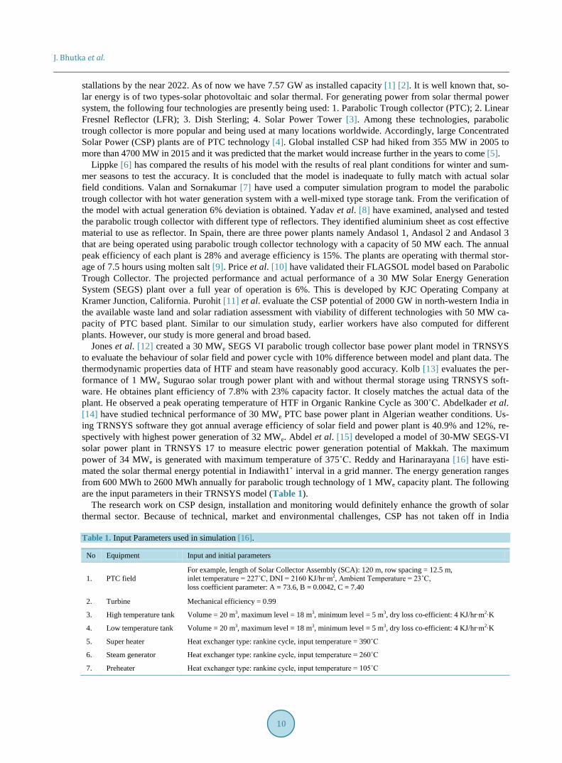
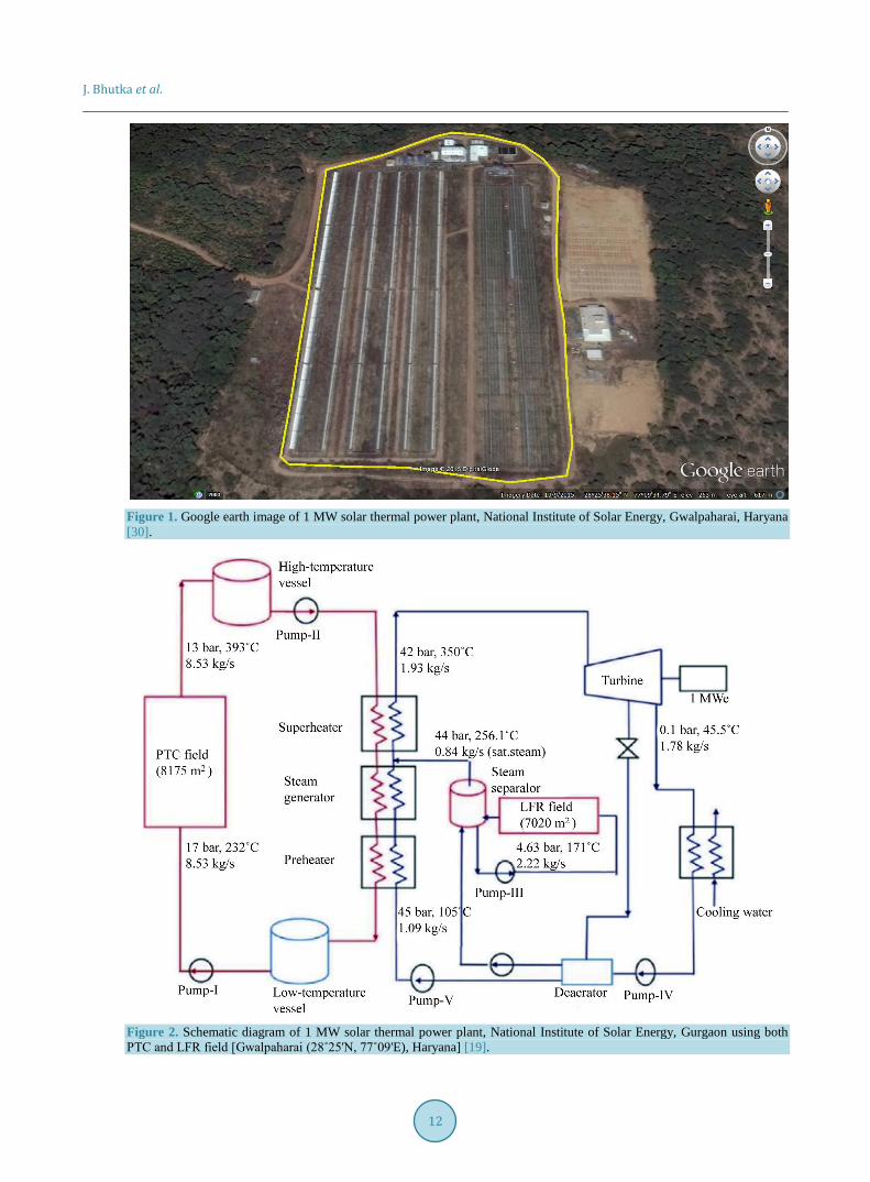
2. Methodology 2.1. 1 MW Solar Thermal Power Plant Details It is known that1 MWe solar thermal power plant is installed in the campus of National Institute of Solar Energy (NISE), Ministry of New and Renewable Energy (MNRE), Government of India (GoI) in Gurgaon at Gwalpa-harai (28˚25'N, 77˚09'E), Haryana, India with full support of Indian Institute of Technology (IIT), Bombay. It is a research cum demonstration plant. The google earth image of plant is shown in Figure 1.

It is using two technologies, Parabolic Trough Collector (PTC) technology and the Linear Fresnel Reflector (LFR) technology. The installed capacity of PTC field is 3 MWth and LFR field is 2 MWth, for a 1 MWe electric output. The Therminol VP 1 is used as Heat Transfer Fluid (HTF) in PTC field and direct saturated steam is used in LFR field. The buffer thermal storage is used for 30 minutes in the form of pressure vessel (High Tem-perature vessel). The PTC field provides 393˚C outlet temperature and 13 bar pressure. The block diagram of the power plant is shown in Figure 2. Here, the fluid heated by the PTC field is stored in high temperature tank. By using HTF pump it is pumped to heat exchanger, where it exchanges heat with the water to generate high tem-perature steam. Later, it is collected in low temperature vessel to store HTF and circulates in solar field. The high temperature steam is directed in the steam turbine to generate the mechanical power and by AC generator it converts into electric power. The exhausted steam from turbine is condensed through condenser and recirculate to generate steam. The LFR field is used to generate saturated steam, which is extracted from the deaerator. The efficiency of PTC field is 43.2% and LFR field is 25.8% with 12% of power unit. The overall plant efficiency is 4.5% [19].

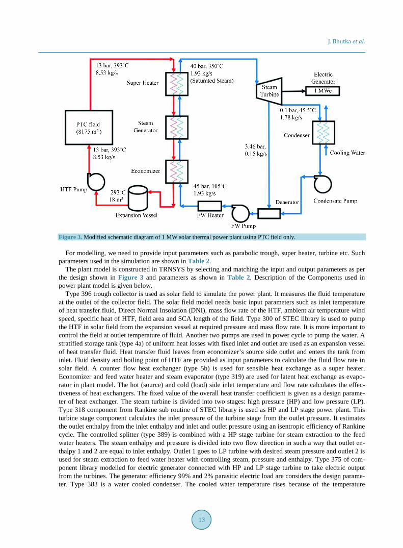
2.2. Simulation of the Plant Model in TRNSYS In our modelling study, the1 MW solar thermal power plant design is changed. This is due to non-availability of LFR field in the user library software. Low temperature and high temperature tanks are used in the plant for buffer storage. We used expansion vessel as a low temperature tank to store and control the HTF flow rate in the solar field. It is worthwhile to simulate the power plant using single technology rather than two technologies for better control. The plant design used in our study is shown in Figure 3 as a simplified line diagram.

J. Bhutka et al.

12

Figure 1. Google earth image of 1 MW solar thermal power plant, National Institute of Solar Energy, Gwalpaharai, Haryana [30].

Figure 2. Schematic diagram of 1 MW solar thermal power plant, National Institute of Solar Energy, Gurgaon using both PTC and LFR field [Gwalpaharai (28˚25'N, 77˚09'E), Haryana] [19].

J. Bhutka et al.

13

Figure 3. Modified schematic diagram of 1 MW solar thermal power plant using PTC field only.

For modelling, we need to provide input parameters such as parabolic trough, super heater, turbine etc. Such

parameters used in the simulation are shown in Table 2. The plant model is constructed in TRNSYS by selecting and matching the input and output parameters as per

the design shown in Figure 3 and parameters as shown in Table 2. Description of the Components used in power plant model is given below.

Type 396 trough collector is used as solar field to simulate the power plant. It measures the fluid temperature at the outlet of the collector field. The solar field model needs basic input parameters such as inlet temperature of heat transfer fluid, Direct Normal Insolation (DNI), mass flow rate of the HTF, ambient air temperature wind speed, specific heat of HTF, field area and SCA length of the field. Type 300 of STEC library is used to pump the HTF in solar field from the expansion vessel at required pressure and mass flow rate. It is more important to control the field at outlet temperature of fluid. Another two pumps are used in power cycle to pump the water. A stratified storage tank (type 4a) of uniform heat losses with fixed inlet and outlet are used as an expansion vessel of heat transfer fluid. Heat transfer fluid leaves from economizer’s source side outlet and enters the tank from inlet. Fluid density and boiling point of HTF are provided as input parameters to calculate the fluid flow rate in solar field. A counter flow heat exchanger (type 5b) is used for sensible heat exchange as a super heater. Economizer and feed water heater and steam evaporator (type 319) are used for latent heat exchange as evapo-rator in plant model. The hot (source) and cold (load) side inlet temperature and flow rate calculates the effec-tiveness of heat exchangers. The fixed value of the overall heat transfer coefficient is given as a design parame-ter of heat exchanger. The steam turbine is divided into two stages: high pressure (HP) and low pressure (LP). Type 318 component from Rankine sub routine of STEC library is used as HP and LP stage power plant. This turbine stage component calculates the inlet pressure of the turbine stage from the outlet pressure. It estimates the outlet enthalpy from the inlet enthalpy and inlet and outlet pressure using an isentropic efficiency of Rankine cycle. The controlled splitter (type 389) is combined with a HP stage turbine for steam extraction to the feed water heaters. The steam enthalpy and pressure is divided into two flow direction in such a way that outlet en-thalpy 1 and 2 are equal to inlet enthalpy. Outlet 1 goes to LP turbine with desired steam pressure and outlet 2 is used for steam extraction to feed water heater with controlling steam, pressure and enthalpy. Type 375 of com-ponent library modelled for electric generator connected with HP and LP stage turbine to take electric output from the turbines. The generator efficiency 99% and 2% parasitic electric load are considers the design parame-ter. Type 383 is a water cooled condenser. The cooled water temperature rises because of the temperature

J. Bhutka et al.

14

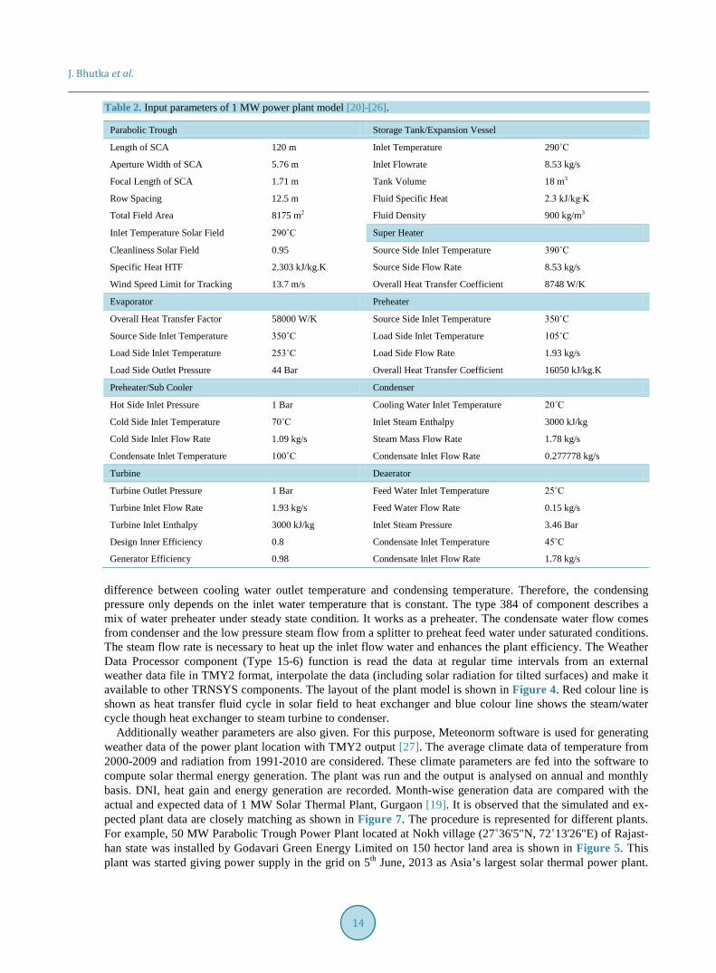
Table 2. Input parameters of 1 MW power plant model [20]-[26].

Parabolic Trough Storage Tank/Expansion Vessel

Length of SCA 120 m Inlet Temperature 290˚C

Aperture Width of SCA 5.76 m Inlet Flowrate 8.53 kg/s

Focal Length of SCA 1.71 m Tank Volume 18 m3

Row Spacing 12.5 m Fluid Specific Heat 2.3 kJ/kg∙K

Total Field Area 8175 m2 Fluid Density 900 kg/m3

Inlet Temperature Solar Field 290˚C Super Heater

Cleanliness Solar Field 0.95 Source Side Inlet Temperature 390˚C

Specific Heat HTF 2.303 kJ/kg.K Source Side Flow Rate 8.53 kg/s

Wind Speed Limit for Tracking 13.7 m/s Overall Heat Transfer Coefficient 8748 W/K

Evaporator Preheater

Overall Heat Transfer Factor 58000 W/K Source Side Inlet Temperature 350˚C

Source Side Inlet Temperature 350˚C Load Side Inlet Temperature 105˚C

Load Side Inlet Temperature 253˚C Load Side Flow Rate 1.93 kg/s

Load Side Outlet Pressure 44 Bar Overall Heat Transfer Coefficient 16050 kJ/kg.K

Preheater/Sub Cooler Condenser

Hot Side Inlet Pressure 1 Bar Cooling Water Inlet Temperature 20˚C

Cold Side Inlet Temperature 70˚C Inlet Steam Enthalpy 3000 kJ/kg

Cold Side Inlet Flow Rate 1.09 kg/s Steam Mass Flow Rate 1.78 kg/s

Condensate Inlet Temperature 100˚C Condensate Inlet Flow Rate 0.277778 kg/s

Turbine Deaerator

Turbine Outlet Pressure 1 Bar Feed Water Inlet Temperature 25˚C

Turbine Inlet Flow Rate 1.93 kg/s Feed Water Flow Rate 0.15 kg/s

Turbine Inlet Enthalpy 3000 kJ/kg Inlet Steam Pressure 3.46 Bar

Design Inner Efficiency 0.8 Condensate Inlet Temperature 45˚C

Generator Efficiency 0.98 Condensate Inlet Flow Rate 1.78 kg/s

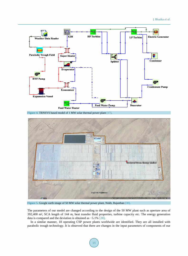
difference between cooling water outlet temperature and condensing temperature. Therefore, the condensing pressure only depends on the inlet water temperature that is constant. The type 384 of component describes a mix of water preheater under steady state condition. It works as a preheater. The condensate water flow comes from condenser and the low pressure steam flow from a splitter to preheat feed water under saturated conditions. The steam flow rate is necessary to heat up the inlet flow water and enhances the plant efficiency. The Weather Data Processor component (Type 15-6) function is read the data at regular time intervals from an external weather data file in TMY2 format, interpolate the data (including solar radiation for tilted surfaces) and make it available to other TRNSYS components. The layout of the plant model is shown in Figure 4. Red colour line is shown as heat transfer fluid cycle in solar field to heat exchanger and blue colour line shows the steam/water cycle though heat exchanger to steam turbine to condenser.

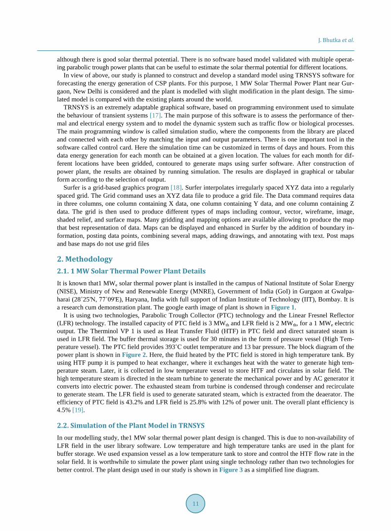
Additionally weather parameters are also given. For this purpose, Meteonorm software is used for generating weather data of the power plant location with TMY2 output [27]. The average climate data of temperature from 2000-2009 and radiation from 1991-2010 are considered. These climate parameters are fed into the software to compute solar thermal energy generation. The plant was run and the output is analysed on annual and monthly basis. DNI, heat gain and energy generation are recorded. Month-wise generation data are compared with the actual and expected data of 1 MW Solar Thermal Plant, Gurgaon [19]. It is observed that the simulated and ex-pected plant data are closely matching as shown in Figure 7. The procedure is represented for different plants. For example, 50 MW Parabolic Trough Power Plant located at Nokh village (27˚36'5"N, 72˚13'26"E) of Rajast-han state was installed by Godavari Green Energy Limited on 150 hector land area is shown in Figure 5. This plant was started giving power supply in the grid on 5th June, 2013 as Asia’s largest solar thermal power plant.

J. Bhutka et al.

15

Figure 4. TRNSYS based model of 1 MW solar thermal power plant [17].

Figure 5. Google earth image of 50 MW solar thermal power plant, Nokh, Rajasthan [30].

The parameters of our model are changed according to the design of the 50 MW plant such as aperture area of 392,400 m², SCA length of 144 m, heat transfer fluid properties, turbine capacity etc. The energy generation data is compared and the deviation is obtained as −5.1% [28].

In a similar manner, 18 operating CSP power plants worldwide are identified. They are all installed with parabolic trough technology. It is observed that there are changes in the input parameters of components of our

J. Bhutka et al.

16

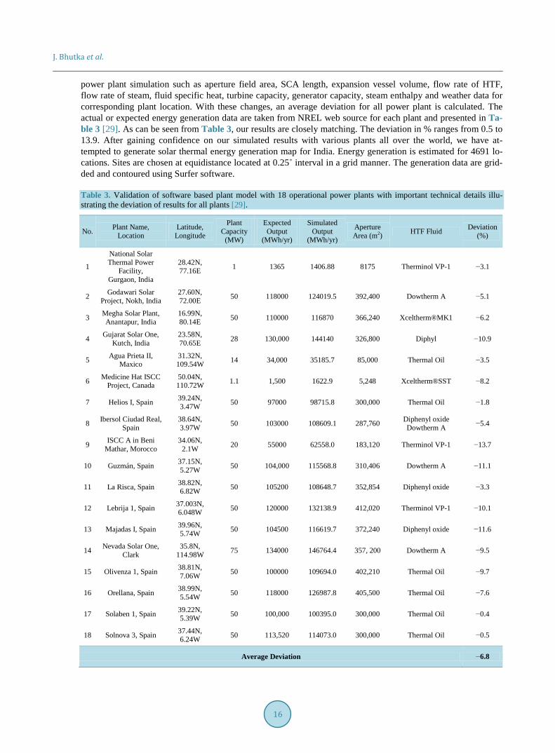
power plant simulation such as aperture field area, SCA length, expansion vessel volume, flow rate of HTF, flow rate of steam, fluid specific heat, turbine capacity, generator capacity, steam enthalpy and weather data for corresponding plant location. With these changes, an average deviation for all power plant is calculated. The actual or expected energy generation data are taken from NREL web source for each plant and presented in Ta-ble 3 [29]. As can be seen from Table 3, our results are closely matching. The deviation in % ranges from 0.5 to 13.9. After gaining confidence on our simulated results with various plants all over the world, we have at-tempted to generate solar thermal energy generation map for India. Energy generation is estimated for 4691 lo-cations. Sites are chosen at equidistance located at 0.25˚ interval in a grid manner. The generation data are grid-ded and contoured using Surfer software.

Table 3. Validation of software based plant model with 18 operational power plants with important technical details illu-strating the deviation of results for all plants [29].

No. Plant Name, Location

Latitude, Longitude

Plant Capacity

(MW)

Expected Output

(MWh/yr)

Simulated Output

(MWh/yr)

Aperture Area (m2) HTF Fluid Deviation

(%)

1

National Solar Thermal Power

Facility, Gurgaon, India

28.42N, 77.16E 1 1365 1406.88 8175 Therminol VP-1 −3.1

2 Godawari Solar Project, Nokh, India

27.60N, 72.00E 50 118000 124019.5 392,400 Dowtherm A −5.1

3 Megha Solar Plant, Anantapur, India

16.99N, 80.14E 50 110000 116870 366,240 Xceltherm®MK1 −6.2

4 Gujarat Solar One, Kutch, India

23.58N, 70.65E 28 130,000 144140 326,800 Diphyl −10.9

5 Agua Prieta II, Maxico

31.32N, 109.54W 14 34,000 35185.7 85,000 Thermal Oil −3.5

6 Medicine Hat ISCC Project, Canada

50.04N, 110.72W 1.1 1,500 1622.9 5,248 Xceltherm®SST −8.2

7 Helios I, Spain 39.24N, 3.47W 50 97000 98715.8 300,000 Thermal Oil −1.8

8 Ibersol Ciudad Real, Spain

38.64N, 3.97W 50 103000 108609.1 287,760 Diphenyl oxide

Dowtherm A −5.4

9 ISCC A in Beni Mathar, Morocco

34.06N, 2.1W 20 55000 62558.0 183,120 Therminol VP-1 −13.7

10 Guzmán, Spain 37.15N, 5.27W 50 104,000 115568.8 310,406 Dowtherm A −11.1

11 La Risca, Spain 38.82N, 6.82W 50 105200 108648.7 352,854 Diphenyl oxide −3.3

12 Lebrija 1, Spain 37.003N, 6.048W 50 120000 132138.9 412,020 Therminol VP-1 −10.1

13 Majadas I, Spain 39.96N, 5.74W 50 104500 116619.7 372,240 Diphenyl oxide −11.6

14 Nevada Solar One, Clark

35.8N, 114.98W 75 134000 146764.4 357, 200 Dowtherm A −9.5

15 Olivenza 1, Spain 38.81N, 7.06W 50 100000 109694.0 402,210 Thermal Oil −9.7

16 Orellana, Spain 38.99N, 5.54W 50 118000 126987.8 405,500 Thermal Oil −7.6

17 Solaben 1, Spain 39.22N, 5.39W 50 100,000 100395.0 300,000 Thermal Oil −0.4

18 Solnova 3, Spain 37.44N, 6.24W 50 113,520 114073.0 300,000 Thermal Oil −0.5

Average Deviation −6.8

J. Bhutka et al.

17

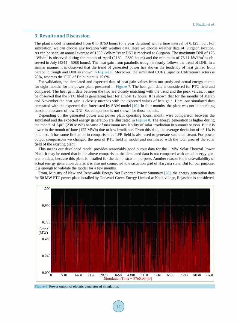
3. Results and Discussion The plant model is simulated from 0 to 8760 hours (one year duration) with a time interval of 0.125 hour. For simulation, we can choose any location with weather data. Here we choose weather data of Gurgaon location. As can be seen, an annual average of 1550 kWh/m2/year DNI is received at Gurgaon. The maximum DNI of 175 kWh/m2 is observed during the month of April (2160 - 2880 hours) and the minimum of 73.11 kWh/m2 is ob-served in July (4344 - 5088 hours). The heat gain from parabolic trough is nearly follows the trend of DNI. In a similar manner it is observed that the trend of generated power has shown the tendency of heat gained from parabolic trough and DNI as shown in Figure 6. Moreover, the simulated CUF (Capacity Utilization Factor) is 20%, whereas the CUF of Delhi plant is 15.6%.

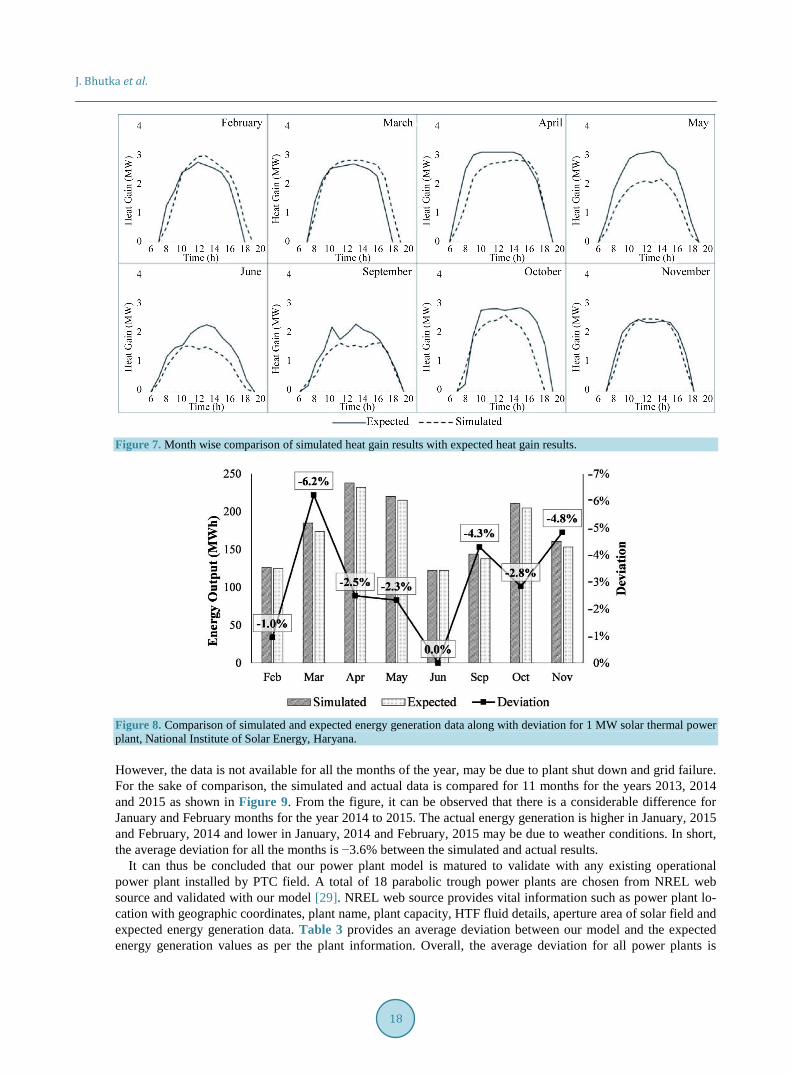
For validation, the simulated and expected data of heat gain values from our study and actual energy output for eight months for the power plant presented in Figure 7. The heat gain data is considered for PTC field and compared. The heat gain data between the two are closely matching with the trend and the peak values. It may be observed that the PTC filed is generating heat for almost 12 hours. It is shown that for the months of March and November the heat gain is closely matches with the expected values of heat gain. Here, our simulated data compared with the expected data forecasted by SAM model [19]. In four months, the plant was not in operating condition because of low DNI. So, comparison is not shown for those months.

Depending on the generated power and power plant operating hours, month wise comparison between the simulated and the expected energy generation are illustrated in Figure 8. The energy generation is higher during the month of April (238 MWh) because of maximum availability of solar irradiation in summer season. But it is lower in the month of June (122 MWh) due to low irradiance. From this data, the average deviation of −3.1% is obtained. It has some limitation in comparison as LFR field is also used to generate saturated steam. For power output comparisom we changed the area of PTC field in model and normlized with the total area of the solar field of the existing plant.

This means our developed model provides reasonably good output data for the 1 MW Solar Thermal Power Plant. It may be noted that in the above comparison, the simulated data is not compared with actual energy gen-eration data, because this plant is installed for the demonstration purpose. Another reason is the unavailability of actual energy generation data as it is also not connected to evacuation grid of Haryana state. But for our purpose, it is enough to validate the model for a few months.

From, Ministry of New and Renewable Energy Net Exported Power Summary [28], the energy generation data for 50 MW PTC power plant installed by Godavari Green Energy Limited at Nokh village, Rajasthan is considered.

Figure 6. Power output of electric generator of simulation.

J. Bhutka et al.

18

Figure 7. Month wise comparison of simulated heat gain results with expected heat gain results.

Figure 8. Comparison of simulated and expected energy generation data along with deviation for 1 MW solar thermal power plant, National Institute of Solar Energy, Haryana.

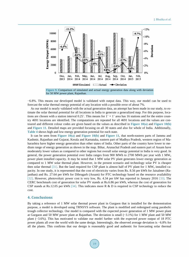
However, the data is not available for all the months of the year, may be due to plant shut down and grid failure. For the sake of comparison, the simulated and actual data is compared for 11 months for the years 2013, 2014 and 2015 as shown in Figure 9. From the figure, it can be observed that there is a considerable difference for January and February months for the year 2014 to 2015. The actual energy generation is higher in January, 2015 and February, 2014 and lower in January, 2014 and February, 2015 may be due to weather conditions. In short, the average deviation for all the months is −3.6% between the simulated and actual results.

It can thus be concluded that our power plant model is matured to validate with any existing operational power plant installed by PTC field. A total of 18 parabolic trough power plants are chosen from NREL web source and validated with our model [29]. NREL web source provides vital information such as power plant lo-cation with geographic coordinates, plant name, plant capacity, HTF fluid details, aperture area of solar field and expected energy generation data. Table 3 provides an average deviation between our model and the expected energy generation values as per the plant information. Overall, the average deviation for all power plants is

J. Bhutka et al.

19

Figure 9. Comparison of simulated and actual energy generation data along with deviation for 50 MW power plant, Rajasthan.

−6.8%. This means our developed model is validated with output data. This way, our model can be used to forecast the solar thermal energy potential of any location with a possible error of about 7%.

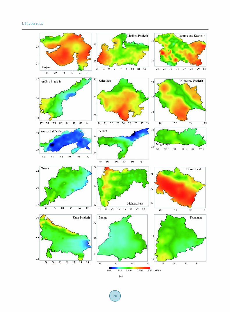
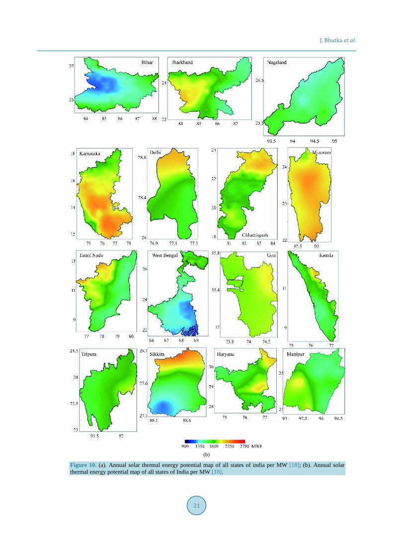
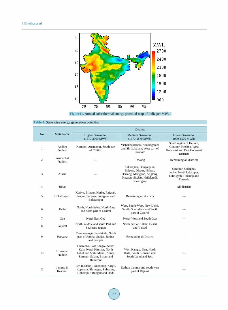
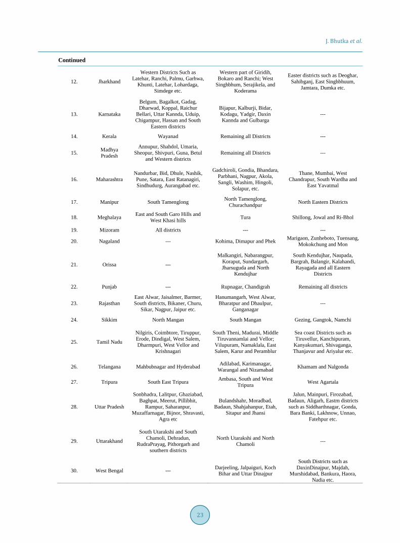
As our model is nearly validated with the actual generation data, an attempt has been made in our study, to es-timate the solar thermal potential for all locations in India to generate a generalized map. For this purpose, loca-tions are chosen with a station interval 0.25˚. This means for 1˚ × 1˚ area has 16 stations and for the entire coun-try 4691 locations are identified. The computations are repeated for all 4691 locations and the values are con-toured and different colour codes are given based on the values as described in Figure 10(a) and Figure 10(b) and Figure 11. Detailed maps are provided focusing on all 30 states and also for whole of India. Additionally, Table 4 shows high and low energy generation potential for each state.

It can be seen from Figure 10(a) and Figure 10(b) and Figure 11, that north-eastern parts of Jammu and Kashmir, Rajasthan and Gujarat, Kerala and Karnataka, eastern part of Madhya Pradesh, western region of Ma-harashtra have higher energy generation than other states of India. Other parts of the country have lower to me-dium range of energy generation as shown in the map. Bihar, Arunachal Pradesh and eastern part of Assam have moderately lower values as compared to other regions but overall solar energy potential in India is very good. In general, the power generation potential over India ranges from 900 MWh to 2700 MWh per year with 1 MWe power plant installed capacity. It may be noted that 1 MW solar PV plant generates lower energy generation as compared to 1 MW solar thermal plant. However, in the present scenario and technology solar PV is cheaper then solar thermal [31]. But the land required for CSP plant is almost half of PV plant for 1 MWe installed ca-pacity. In one study, it is represented that the cost of electricity varies from Rs. 8.56 per kWh for Jaisalmer (Ra-jasthan) and Rs. 27.64 per kWh for Dibrugarh (Assam) for PTC technology based on the resource availability [32]. However, photovoltaic power cost is very low, Rs. 4.34 per kW has reported in January 2016 [33]. The CERC benchmark cost of generation for solar PV stands at Rs.6.86 per kWh, whereas the cost of generation for CSP stands at Rs.12.05 per kWh [34]. This indicates more R & D is required in CSP technology to reduce the cost.

4. Conclusions By taking a reference of 1 MW solar thermal power plant in Gurgaon that is installed for the demonstration purpose, a model is developed using TRNSYS software. The plant is modified and redesigned using parabolic trough collector technology. Our model is compared with the expected power generation of 1 MW power plant at Gurgaon and 50 MW power plant at Rajasthan. The deviation is small (−3.1%) for 1 MW plant and 50 MW plant (−3.6%). This has motivated to validate our model further with the expected power output of 18 PTC power plants all over the world with the same design. Interestingly, the observed average deviation is −6.8% for all the plants. This confirms that our design is reasonably good and authentic for forecasting solar thermal

J. Bhutka et al.

20

(a)

J. Bhutka et al.

21

(b)

Figure 10. (a). Annual solar thermal energy potential map of all states of india per MW [18]; (b). Annual solar thermal energy potential map of all states of India per MW [18].

J. Bhutka et al.

22

Figure11. Annual solar thermal energy potential map of India per MW.

Table 4. State wise energy generation potential.

No. State Name District

Higher Generation (1870-2700 MWh)

Medium Generation (1570-1870 MWh)

Lower Generation (900-1570 MWh)

1. Andhra Pradesh

Kurnool, Anantapur, South part of Chittor,

Vishakhapatnam, Vizinagaram and Shrikakulam, West part of

Praksam

South region of Hellore, Guntour, Krishna, West

Godawari and East Godawari Districts

2. Arunachal Pradesh --- Tawang Remaining all districts

3. Assam ---

Kakarajhar, Bongaigaon, Balpeta, Dispur, Nilbari,

Darrang, Merigaon, Anglong, Nagaon, Silchar, Hailakandi,

Karimganj

Sonitpur, Golaghat, Jorhat, North Lakimpur, Dibrugrah, Dhemaji and

Tinsukia

4. Bihar --- --- All districts

5. Chhattisgarh Koriya, Bilapur, Korba, Raigrah, Jaspur, Surguja, Surajpurs and

Balarampur Remaining all districts ---

6. Delhi North, North-West, North-East and north part of Central

West, South-West, New Delhi, South, South-East and South

part of Central ---

7. Goa North East Goa North-West and South Goa ---

8. Gujarat North, middle and south Part and Saurastra region

North part of Katchh Desert and Valsad ---

9. Haryana Yamunanagar, Panchkula, North

part of Ambla, Jhajjar, Rothar and Sonipat

Remaining all District ---

10. Himachal Pradesh

Chambha, East Kangra, South Kula, North Kinnaur, North

Lahul and Spiti, Mandi, Simla, Sirmaur, Solam, Bispur and

Hamirpur

West Kangra, Una, North Kula, South Kinnaur, and

South Lahul and Spiti ---

11. Jammu & Kashmir

Leh (Ladakh), Anantnag, Kargil, Kupwara, Shrinagar, Pulwama, Udhampur, Budgamand Doda

Kathua, Jammu and south west part of Rajauri ---

J. Bhutka et al.

23

Continued

12. Jharkhand

Western Districts Such as Latehar, Ranchi, Palmu, Garhwa,

Khunti, Latehar, Lohardaga, Simdege etc.

Western part of Giridih, Bokaro and Ranchi; West

Singhbhum, Serajikela, and Koderama

Easter districts such as Deoghar, Sahibganj, East Singhbhuum,

Jamtara, Dumka etc.

13. Karnataka

Belgum, Bagalkot, Gadag, Dharwad, Koppal, Raichur

Bellari, Uttar Kannda, Uduip, Chigampur, Hassan and South

Eastern districts

Bijapur, Kalburji, Bidar, Kodagu, Yadgir, Daxin Kannda and Gulbarga

---

14. Kerala Wayanad Remaining all Districts ---

15. Madhya Pradesh

Annupur, Shahdol, Umaria, Sheopur, Shivpuri, Guna, Betul

and Western districts Remaining all Districts ---

16. Maharashtra Nandurbar, Bid, Dhule, Nashik, Pune, Satara, East Ratanagiri, Sindhudurg, Aurangabad etc.

Gadchiroli, Gondia, Bhandara, Parbhani, Nagpur, Akola, Sangli, Washim, Hingoli,

Solapur, etc.

Thane, Mumbai, West Chandrapur, South Wardha and

East Yavatmal

17. Manipur South Tamenglong North Tamenglong, Churachandpur North Eastern Districts

18. Meghalaya East and South Garo Hills and West Khasi hills Tura Shillong, Jowal and Ri-Bhol

19. Mizoram All districts --- ---

20. Nagaland --- Kohima, Dimapur and Phek Marigaon, Zunheboto, Tuensang, Mokokchung and Mon

21. Orissa ---

Malkangiri, Nabarangpur, Koraput, Sundargarh, Jharsuguda and North

Kendujhar

South Kendujhar, Naupada, Bargrah, Balangir, Kalahandi,

Rayagada and all Eastern Districts

22. Punjab --- Rupnagar, Chandigrah Remaining all districts

23. Rajasthan East Alwar, Jaisalmer, Barmer, South districts, Bikaner, Churu,

Sikar, Nagpur, Jaipur etc.

Hanumangarh, West Alwar, Bharatpur and Dhaulpur,

Ganganagar ---

24. Sikkim North Mangan South Mangan Gezing, Gangtok, Namchi

25. Tamil Nadu

Nilgiris, Coimbtore, Tiruppur, Erode, Dindigal, West Salem, Dharmpuri, West Vellor and

Krishnagari

South Theni, Madurai, Middle Tiruvannamlai and Vellor;

Vilupuram, Namaklala, East Salem, Karur and Peramblur

Sea coast Districts such as Tiruvellur, Kanchipuram,

Kanyakumari, Shivaganga, Thanjavur and Ariyalur etc.

26. Telangana Mahbubnagar and Hyderabad Adilabad, Karimanagar, Warangal and Nizamabad Khamam and Nalgonda

27. Tripura South East Tripura Ambasa, South and West Tripura West Agartala

28. Uttar Pradesh

Sonbhadra, Lalitpur, Ghaziabad, Baghpat, Meerut, Pillibhit,

Rampur, Saharanpur, Muzaffarnagar, Bijnor, Shravasti,

Agra etc

Bulandshahr, Moradbad, Badaun, Shahjahanpur, Etah,

Sitapur and Jhansi

Jalun, Mainpuri, Firozabad, Badaun, Aligarh, Eastrn districts such as Siddharthnagar, Gonda, Bara Banki, Lakhnow, Unnao,

Fatehpur etc.

29. Uttarakhand

South Utarakshi and South Chamoli, Dehradun,

RudraPrayag, Pithorgarh and southern districts

North Utarakshi and North Chamoli ---

30. West Bengal --- Darjeeling, Jalpaiguri, Koch Bihar and Uttar Dinajpur

South Districts such as DaxinDinajpur, Majdah,

Murshidabad, Bankura, Haora, Nadia etc.

J. Bhutka et al.

24

potential of any location. The reason for deviation may be due to Meteonorm based weather data which may be different from the actual weather data and also due to minor differences in the plant design from the exact design of a particular plant.

After getting confidence on our computation and model validity with actual generation, we have also ex-tended our study at 4691 stations at different locations of India with a station interval of 0.25˚ × 0.25˚ spacing in a grid manner. This has facilitated to prepare maps of monthly and annual energy generation for all the 30 states of India and thus for the whole country. Based on these maps, high and low energy potential districts of each state are tabulated. Our results in the form of maps will form as a basis and served as solar thermal atlas, which is first of its kind in India. However, no claim is made that our maps are final. Further improvement of these maps can be made with new information and new data.

Acknowledgements Authors would like to thank Sri J. N. Singh, VCMT of Gujarat Energy Research & Management Institute (GERMI), Gandhinagar, for being constant source of inspiration and encouraging us to share our knowledge and experience in the form of publication for greater benefit of the solar industry in India and abroad. We also ap-preciate GERMI management for providing necessary software for conducting this study. Special thanks goes to SriPrashant Gopiyani, the project intern coordinator during execution of the project.

References [1] Ministry of New and Renewable Energy, Government of India (2014) Jawaharlal Nehru National Solar Mission.

http://www.mnre.gov.in/solar-mission/jnnsm/introduction-2 [2] http://www.mnre.gov.in/mission-and-vision-2/achievements/ [3] Sukhatme, S. and Nayak, J. (2009) Solar Energy: Principles of Thermal Collection and Storage. 3rd Edition, Tata

McGraw Hill, New York. [4] https://en.wikipedia.org/wiki/List_of_solar_thermal_power_station [5] http://social.csptoday.com/markets/global-csp-capacity-forecast-hit-22-gw-2025 [6] Lippke, F. (1995) Simulation of the Part-Load Behaviour of a 30 MWe SEGS Plant, SAND95-1293, Sandia National

Laboratories, Albuquerque, NM. http://dx.doi.org/10.2172/95571 [7] Valan, A. and Sornakumar, S. (2007) Theoretical Analysis and Experimental Verification of Parabolic Trough Solar

Collector with Hot Water Generation System. THERMAL SCIENCE, 11, 119-126. http://dx.doi.org/10.2298/TSCI0701119V

[8] Yadav, A., Kumar, M. and Balram (2003) Experimental Study and Analysis of Parabolic Trough Collector with Vari-ous Reflectors. International Journal of Mathematical, Computational, Physical, Electrical and Computer Engineering, 7, 1663-1667.

[9] Solar Millennium, A.G. (2008) The Parabolic Trough Power Plants Andasol 1-3. The Largest Solar Power Plant in the World-Technology Premiere in Europe. https://www.rwe.com/web/cms/mediablob/en/1115150/data/0/1/Further-information-about-Andasol.pdf

[10] Price, H., Svoboda, P. and Kearney, D. (1995) Validation of the FLAGSSOL Parabolic Trough Solar Power Plant Per-formance Model. International Solar Energy Conference, Maui, 19-24 March 1995, HI. http://www.osti.gov/scitech/servlets/purl/36778

[11] Purohit, I., Purohit, P. and Shekhar, S. (2013) Evaluating the Potential of Concentrating Solar Power Generation in North-Western India. Energy Policy, 62, 157-175. http://dx.doi.org/10.1016/j.enpol.2013.06.069

[12] Jones, S., Pitz-Paal, R., Schwarzboezl, P., Blair, N. and Cable, R. (2001) TRNSYS Modelling of the SEGS VI Para-bolic Trough Solar Electric Generating System. ASME International Solar Energy Conference Solar Forum, Washing-ton DC. http://catalog.asme.org/ConferencePublications/PrintBook/2001_Solar_Proceedings_Intl.cfm

[13] Kolb, G. and Hassani, V. (2006) Performance Analysis of Thermocline Energy Storage Proposed for the 1 MW Sa-guaro Solar Trough Plant. ASME International Solar Energy Conference, Denver, 8-13 July 2006, 1-5. http://dx.doi.org/10.1115/isec2006-99005

[14] Abdelkader, Z., Mohamed, Y. and Noureddine, S. (2012) Technical and Economical Performance of Parabolic Trough Collector Power Plant under Algerian Climate. Procedia Engineering, 33, 78-91. http://dx.doi.org/10.1016/j.proeng.2012.01.1179

[15] Abdel, D., Nabil, M., Alghamdi, S. and Marzouk, E. (2013) Potential of Solar Thermal Energy Utilization in Electrical

J. Bhutka et al.

25

Generation.2nd International Conference on Energy Systems and Technologies, Cairo, 18-21 February 2013, 177-188. [16] Nagarjuna Reddy, C. and Harinarayana, T. (2015) Solar Thermal Energy Generation Potential in Gujarat and Tamil

Nadu States, India. Energy and Power Engineering, 7, 591-603. http://dx.doi.org/10.4236/epe.2015.713056 [17] TRNSYS 17. http://www.trnsys.com/ [18] Surfer 13. www.goldensoftware.com/products/surfer [19] Nayak, J., Kedare, S., Banerjee, R., Bandyopadhyay, S., Desai, N., Paul, S. and Kapila, A. (2015) A 1MW National

Solar Thermal Research Cum Demonstration Facility at Gwalpahari, Haryana, India. Current Science, 109, 1445-1457. http://www.currentscience.ac.in/Volumes/109/08/1445.pdf http://dx.doi.org/10.18520/cs/v109/i8/1445-1457

[20] Xu, E., Zhao, D., Xu, H., Li, S., Zhang, Z., Wang, Z. and Wang, Z. (2015) The Badaling 1MW Parabolic Trough Solar Thermal Power Pilot Plant. International Conference on Concentrating Solar Power and Chemical Energy Systems, 69, 1471-1478. http://www.sciencedirect.com/science/article/pii/S1876610215004026 http://dx.doi.org/10.1016/j.egypro.2015.03.096

[21] Geyer, M., Lüpfert, E., Osuna, R., Esteban, A., Schiel, W., Schweitzer, A., Zarza, E., Nava, P., Langenkamp, J. and Mandelberg, E. (2002) EUROTROUGH—Parabolic Trough Collector Developed for Cost Efficient Solar Power Gen-eration.11th SolarPACES International Symposium on Concentrated Solar Power and Chemical Energy Technologies, Zurich, 4-6 September 2002, 1-7. http://www.fika.org/jb/resources/EuroTrough.pdf

[22] Solutia Inc (2001) A Selection Guide THERMINOL VP-1 12˚C to 400 ˚C Heat Transfer Fluids. http://twt.mpei.ac.ru/tthb/hedh/htf-vp1.pdf

[23] http://www.turbinesinfo.com/types-of-steam-turbines/ [24] http://www.nise.res.in/PDF_NISE/EOI-of-1MW-Power-Plant-at-NISE.pdf [25] Kumar, A., Chand, S. and Umrao, O. (2001) Design and Analysis for 1MWe Parabolic Trough Solar Collector Plant

Based on DSG Method. Solar Energy Forum: The Power to Choose, Washington DC. http://sel.me.wisc.edu/trnsys/trnlib/stec/jones_et_al.pdf

[26] Jones, S., Pitz-Paal, R., Schwarzboezl, P., Blair, N. and Cable, R. (2001) TRNSYS Modelling of the SEGS VI Para-bolic Trough Solar Electric Generating System. ASME International Solar Energy Conference Solar Forum, Washing-ton DC, 21-25 April 2001. http://sel.me.wisc.edu/trnsys/trnlib/stec/jones_et_al.pdf

[27] METEONORM 7(2015) http://meteonorm.com [28] http://mnre.gov.in/file-manager/UserFiles/net-exported-solar-power-summary.htm (2015) [29] http://www.nrel.gov/csp/solarpaces/parabolic_trough.cfm [30] Google Earth (2016) https://www.google.com/earth/ [31] Harinarayana, T. and Jaya Kashyap, K. (2014) Solar Energy Generation Potential Estimation in India and Gujarat,

Andhra, Telangana States. Smart Grid and Renewable Energy, 5, 275-289. http://dx.doi.org/10.4236/sgre.2014.511025 [32] Purohit, I. and Purohit, P. (2010) Techno-Economic Evaluation of Concentrating Solar Power Generation in India. En-

ergy Policy, 38, 3015-3029. http://dx.doi.org/10.1016/j.enpol.2010.01.041 http://www.sciencedirect.com/science/article/pii/S0301421510000698

[33] http://timesofindia.indiatimes.com/india/Rs-4-34-a-unit-Solar-power-tariff-drops-to-record-low/articleshow/50643394.cms

[34] Central Electricity Regulatory Commission (2014) Determination of Generic Levellised Generation Tariff for the FY 2014-15 under Regulation 8 of the Central Electricity Regulatory Commission. Central Electricity Regulatory Com-mission, New Delhi.

Submit or recommend next manuscript to SCIRP and we will provide best service for you: Accepting pre-submission inquiries through Email, Facebook, LinkedIn, Twitter, etc. A wide selection of journals (inclusive of 9 subjects, more than 200 journals) Providing 24-hour high-quality service User-friendly online submission system Fair and swift peer-review system Efficient typesetting and proofreading procedure Display of the result of downloads and visits, as well as the number of cited articles Maximum dissemination of your research work

Submit your manuscript at: http://papersubmission.scirp.org/