Bachelor Thesis Chemistry

Modeling oil paint network formationfor characterization of the molecular

topology

Jorien Duivenvoorden1

Supervisors: dr. I. Kryven1, prof. dr. P.D. Iedema1 and dr. C. Fonseca Guerra2

1 Paint Alterations in Time,Van ’t Hoff Institute for Molecular Sciences, University of Amsterdam

and The Rijksmuseum, Amsterdam2 Computational Biochemistry and Molecular Recognition

Division of Theoretical ChemistryFree University Amsterdam

!

!

Bachelor Thesis Scheikunde

Modeling oil paint network formation and the

characterization of the molecular topology

door

Jorien Duivenvoorden  

2 juli 2015  

Studentnummer 10431810

Onderzoeksinstituut HIMS Onderzoeksgroep PAinT

Verantwoordelijk docent Prof. dr. P.D. Iedema Begeleider Dr. I. Kryven

Abstract

Oil paintings and their degradation is a popular topic of research. However,cured, or polymerized, oil paint is a strongly cross-linked polymer and analysisof the structure of the network is practically impossible because of this. Insightin the structure is necessary to explain several degradation processes, such as themigration of metal ions, that are not fully understood thus far. In this study theonly option to obtain structural information about the molecular topology of an oilpaint network after polymerization is employed; an advanced model is developed thatsimulates the formation of an oil paint network. Because this challenge has not beenaddressed until now, we looked for the methodology to other fields of research. Weemployed a kind of Gillespie Monte Carlo method in combination with graph theory,a mathematical approach to describe the connectivity of a network. The monomersof an oil paint polymer are triacylglycerides (TAG-units), which contain doublebonds that are responsible for the formation of the cross-links. The starting point ofthe model is the assumption that the reactivity of these monomers only depends ontheir number of double bonds, or their functionality. This is the main assumptionfrom polymer reaction engineering and the application to oil paint is already anovelty. Oil paint monomers can have a functionality up to 9, which is considerablymore than most industrial monomers. Because of this and when no other effectsthat influence the reactivity of the monomers are taken into account, the networkbecomes too dense. Therefore, we added three novel advanced routines to approacha realistic chemical system more accurately. Preferential coupling, the first effect,ensures that monomers that are close together will connect with a high probability.Secondly, intramolecular bonds within a TAG-unit are allowed. The third effectis steric hindrance and implies that shielded monomers have a low probability ofconnecting. The final part of this research is about the validation of the model.An experiment is designed within the research group and we wrote an algorithm tosimulate this experiment. The goal of the experiment is to break the network intopieces by hydrolyzing the TAG-units. The original cross-links are retained in thesefragments that can be analyzed. The experimental results can be coupled to themodel to find the original network and all its structural information.

3

Dutch summary

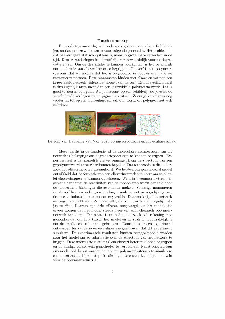
Er wordt tegenwoordig veel onderzoek gedaan naar olieverfschilderi-jen, omdat men ze wil bewaren voor volgende generaties. Het probleem isdat olieverf geen statisch systeem is, maar in grote mate verandert in detijd. Deze veranderingen in olieverf zijn verantwoordelijk voor de degra-datie ervan. Om de degradatie te kunnen voorkomen, is het belangrijkom de chemie van olieverf beter te begrijpen. Olieverf is een polymeer-systeem, dat wil zeggen dat het is opgebouwd uit bouwstenen, die wemonomeren noemen. Deze monomeren binden met elkaar en vormen eeningewikkeld netwerk tijdens het drogen van de verf. Een olieverfschilderijis dus eigenlijk niets meer dan een ingewikkeld polymeernetwerk. Dit isgoed te zien in de figuur. Als je inzoomt op een schilderij, zie je eerst deverschillende verflagen en de pigmenten zitten. Zoom je vervolgens nogverder in, tot op een moleculaire schaal, dan wordt dit polymeer netwerkzichtbaar.

De tuin van Daubigny van Van Gogh op microscopische en moleculaire schaal.

Meer inzicht in de topologie, of de moleculaire architectuur, van ditnetwerk is belangrijk om degradatieprocessen te kunnen begrijpen. Ex-perimenteel is het namelijk vrijwel onmogelijk om de structuur van eengepolymerizeerd netwerk te kunnen bepalen. Daarom wordt in dit onder-zoek het olieverfnetwerk gesimuleerd. We hebben een geavanceerd modelontwikkeld dat de formatie van een olieverfnetwerk simuleert om zo aller-lei eigenschappen te kunnen ophelderen. We zijn begonnen met een al-gemene aanname: de reactiviteit van de monomeren wordt bepaald doorde hoeveelheid bindingen die ze kunnen maken. Sommige monomerenin olieverf kunnen wel negen bindingen maken, wat in vergelijking metde meeste industrile monomeren erg veel is. Daarom krijgt het netwerkeen erg hoge dichtheid. Zo hoog zelfs, dat dit fysisch niet mogelijk bli-jkt te zijn. Daarom zijn drie effecten toegevoegd aan het model, dieervoor zorgen dat het model steeds meer een echt chemisch polymeer-netwerk benaderd. Ten slotte is er in dit onderzoek ook rekening meegehouden dat een link tussen het model en de realiteit noodzakelijk isom de resultaten te kunnen gebruiken. Daarom is er een experimentontworpen ter validatie en een algoritme geschreven dat dit experimentsimuleert. De experimentele resultaten kunnen teruggekoppeld wordennaar het model om zo informatie over de structuur van het netwerk tekrijgen. Deze informatie is cruciaal om olieverf beter te kunnen begrijpenen de huidige conserveringsmethodes te verbeteren. Naast olieverf, kanons model ook benut worden om andere polymeersystemen te simuleren;een onverwachte bijkomstigheid die erg interessant kan blijken te zijnvoor de polymeerindustrie.

4

Contents

1 Introduction 51.1 Oil paint network and its characterization . . . . . . . . . 51.2 Research context . . . . . . . . . . . . . . . . . . . . . . . 61.3 Introduction to graph theory . . . . . . . . . . . . . . . . 7

2 Standard model 102.1 Simulation details . . . . . . . . . . . . . . . . . . . . . . 102.2 Gillespie Monte Carlo . . . . . . . . . . . . . . . . . . . . 112.3 Post-processing . . . . . . . . . . . . . . . . . . . . . . . . 13

2.3.1 Component size distribution . . . . . . . . . . . . . 132.3.2 Gel fraction . . . . . . . . . . . . . . . . . . . . . . 132.3.3 Gel point . . . . . . . . . . . . . . . . . . . . . . . 132.3.4 Degree distribution . . . . . . . . . . . . . . . . . . 142.3.5 Cyclomatic number . . . . . . . . . . . . . . . . . 142.3.6 Average shortest path . . . . . . . . . . . . . . . . 142.3.7 Clustering coefficient . . . . . . . . . . . . . . . . . 142.3.8 Number of triangles . . . . . . . . . . . . . . . . . 152.3.9 Linear size distribution . . . . . . . . . . . . . . . 152.3.10 Community distribution . . . . . . . . . . . . . . . 162.3.11 Dispersity . . . . . . . . . . . . . . . . . . . . . . . 16

2.4 Discussion of the results . . . . . . . . . . . . . . . . . . . 17

3 Advanced network formation 223.1 Preferential coupling . . . . . . . . . . . . . . . . . . . . . 22

3.1.1 Discussion of the results . . . . . . . . . . . . . . . 233.2 Intramolecular bonds . . . . . . . . . . . . . . . . . . . . . 30

3.2.1 Discussion of the results . . . . . . . . . . . . . . . 303.3 Shielding . . . . . . . . . . . . . . . . . . . . . . . . . . . 32

4 Validation of the model 33

5 Conclusion 37

6 Prospects 39

7 Acknowledgments 39

Appendices 40

References 44

4

1 Introduction

1.1 Oil paint network and its characterization

Since oil paint has first been discovered by Van Eyck in the early fif-teenth century, it is has been a widely used paint medium for many yearsto come. Whether Van Eyck really was the first to use oil paint is dis-putable, but art historians do agree on the boost that the use of oil paintexperienced from this moment onwards.1 Historically, oil paintings arepainted with drying oils such as linseed, walnut and poppy seed oils.2 Inthe drying process of these oils no solvent evaporates, but the chemicalstructure of the oil changes.3 Would Van Eyck have known that oil paintis actually a dense, entangled network made from cross-linked buildingblocks that we call monomers? Probably not.

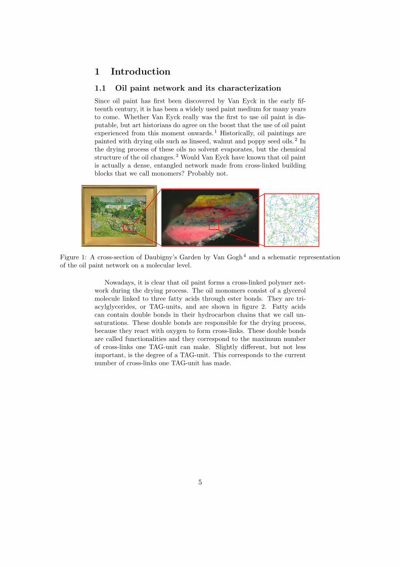
Figure 1: A cross-section of Daubigny’s Garden by Van Gogh4 and a schematic representationof the oil paint network on a molecular level.

Nowadays, it is clear that oil paint forms a cross-linked polymer net-work during the drying process. The oil monomers consist of a glycerolmolecule linked to three fatty acids through ester bonds. They are tri-acylglycerides, or TAG-units, and are shown in figure 2. Fatty acidscan contain double bonds in their hydrocarbon chains that we call un-saturations. These double bonds are responsible for the drying process,because they react with oxygen to form cross-links. These double bondsare called functionalities and they correspond to the maximum numberof cross-links one TAG-unit can make. Slightly different, but not lessimportant, is the degree of a TAG-unit. This corresponds to the currentnumber of cross-links one TAG-unit has made.

5

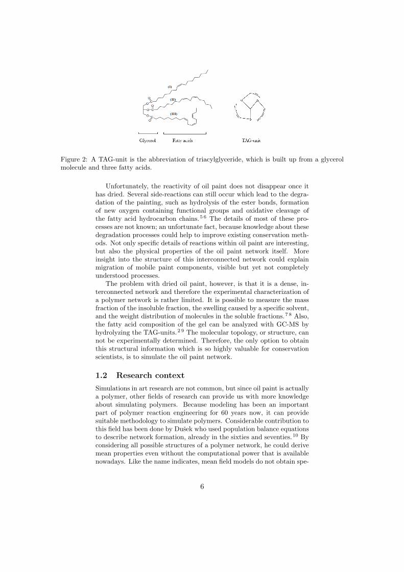
Figure 2: A TAG-unit is the abbreviation of triacylglyceride, which is built up from a glycerolmolecule and three fatty acids.

Unfortunately, the reactivity of oil paint does not disappear once ithas dried. Several side-reactions can still occur which lead to the degra-dation of the painting, such as hydrolysis of the ester bonds, formationof new oxygen containing functional groups and oxidative cleavage ofthe fatty acid hydrocarbon chains.5 6 The details of most of these pro-cesses are not known; an unfortunate fact, because knowledge about thesedegradation processes could help to improve existing conservation meth-ods. Not only specific details of reactions within oil paint are interesting,but also the physical properties of the oil paint network itself. Moreinsight into the structure of this interconnected network could explainmigration of mobile paint components, visible but yet not completelyunderstood processes.

The problem with dried oil paint, however, is that it is a dense, in-terconnected network and therefore the experimental characterization ofa polymer network is rather limited. It is possible to measure the massfraction of the insoluble fraction, the swelling caused by a specific solvent,and the weight distribution of molecules in the soluble fractions.7 8 Also,the fatty acid composition of the gel can be analyzed with GC-MS byhydrolyzing the TAG-units.2 9 The molecular topology, or structure, cannot be experimentally determined. Therefore, the only option to obtainthis structural information which is so highly valuable for conservationscientists, is to simulate the oil paint network.

1.2 Research context

Simulations in art research are not common, but since oil paint is actuallya polymer, other fields of research can provide us with more knowledgeabout simulating polymers. Because modeling has been an importantpart of polymer reaction engineering for 60 years now, it can providesuitable methodology to simulate polymers. Considerable contribution tothis field has been done by Dusek who used population balance equationsto describe network formation, already in the sixties and seventies.10 Byconsidering all possible structures of a polymer network, he could derivemean properties even without the computational power that is availablenowadays. Like the name indicates, mean field models do not obtain spe-

6

cific topologies, but only mean properties, because no distinction is madebetween different monomers.11 12 13 Importantly, Dusek did adjust theprobability of connecting monomers in such a way that not all monomershave the same chance of connecting.14 A mean field model is one wayto describe a network, but there are several alternatives. They can besubdivided in in three groups: mean field models, percolation models andkinetic Monte Carlo models. Compared to mean field, percolation mod-els make more use of topologies, although constrained on a grid. Thisdoes mean that percolation models have three dimensions and thereforeprovide spatial information.

The third group is the kinetic Monte Carlo method, which is a prob-abilistic method that allows the following of the growth of individualchains as a function of time and/or conversion by jumping from onestate to another according to a certain probability. A drawback of thismethod is its high computational requirements. The definition of such astate can be a property, such as a size distribution of polymer units.15

Recently, Hamzehlou et al. have made a contribution to this field bytaking a topology as the state on which the simulation is based. Usingtheir model the conversion evolution of the entire molecular weight distri-bution, the cross-linking density distribution and available double bonddensity distribution before and after gel point can be determined in con-trast to earlier models that could only give detailed information beforethe gel point. Surprisingly, the only structural information this modeloffers is the chain length between two branching points, the distributionof chains with a given chain length and cross-linking density.7 Particu-larly, this structural information that can be extracted from topologies ishighly interesting for conservation scientists, since it cannot be extractedfrom actual oil paint and, more importantly, it explains several processesin the oil paint that lead to degradation such as the formation of metalsoaps.

The hiatus in the field of theoretical descriptions of polymer networkslies in the combination of the work of Dusek and Hamzehlou et al. andthis is exactly where this study is focused on. The topologies obtainedby a kinetic Monte Carlo model employed by Hamzehlou et al. providestructural information that can be used to adjust the probability of cer-tain monomers to connect, just as Dusek did. Only now, the monomerscan be treated separately, because all the information needed for this isprovided by the topologies. A start has been made by Meimaroglou andKiparissides who take steric hindrance into account with their combinedstochastic kinetic/topology algorithm.16 This study will advance furtherinto the field of kinetic Monte Carlo topology models with the use ofgraph theory, which proves to be very suitable for this.17

1.3 Introduction to graph theory

In this study the oil paint network is described using graph theory. Graphtheory employs mathematical structures to describe connections in a net-work. These networks can range from your friends on Facebook, to theWorld Wide Web and to neurological networks in your brain.18 In the

7

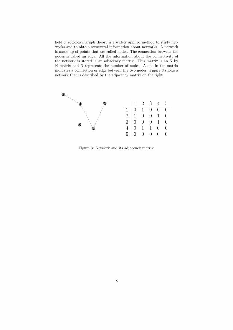
field of sociology, graph theory is a widely applied method to study net-works and to obtain structural information about networks. A networkis made up of points that are called nodes. The connection between thenodes is called an edge. All the information about the connectivity ofthe network is stored in an adjacency matrix. This matrix is an N byN matrix and N represents the number of nodes. A one in the matrixindicates a connection or edge between the two nodes. Figure 3 shows anetwork that is described by the adjacency matrix on the right.

Figure 3: Network and its adjacency matrix.

8

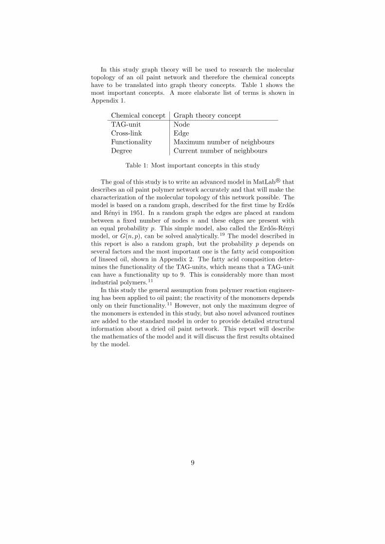
In this study graph theory will be used to research the moleculartopology of an oil paint network and therefore the chemical conceptshave to be translated into graph theory concepts. Table 1 shows themost important concepts. A more elaborate list of terms is shown inAppendix 1.

Chemical concept Graph theory concept

TAG-unit NodeCross-link EdgeFunctionality Maximum number of neighboursDegree Current number of neighbours

Table 1: Most important concepts in this study

The goal of this study is to write an advanced model in MatLab R© thatdescribes an oil paint polymer network accurately and that will make thecharacterization of the molecular topology of this network possible. Themodel is based on a random graph, described for the first time by Erdosand Renyi in 1951. In a random graph the edges are placed at randombetween a fixed number of nodes n and these edges are present withan equal probability p. This simple model, also called the Erdos-Renyimodel, or G(n, p), can be solved analytically.19 The model described inthis report is also a random graph, but the probability p depends onseveral factors and the most important one is the fatty acid compositionof linseed oil, shown in Appendix 2. The fatty acid composition deter-mines the functionality of the TAG-units, which means that a TAG-unitcan have a functionality up to 9. This is considerably more than mostindustrial polymers.11

In this study the general assumption from polymer reaction engineer-ing has been applied to oil paint; the reactivity of the monomers dependsonly on their functionality.11 However, not only the maximum degree ofthe monomers is extended in this study, but also novel advanced routinesare added to the standard model in order to provide detailed structuralinformation about a dried oil paint network. This report will describethe mathematics of the model and it will discuss the first results obtainedby the model.

9

2 Standard model

2.1 Simulation details

We developed a model, in which we applied the main assumption frompolymer reaction engineering to oil paint and we call it the standardmodel. The information about the simulated network is stored in adja-cency matrix A. Matrix A describes the connectivity of the network andit is important to realize that matrix A and the topology of the networkcontain exactly the same information.

A = ai,j =

{1 if nodes i and j are connected

0 if nodes i and j are not connected(1)

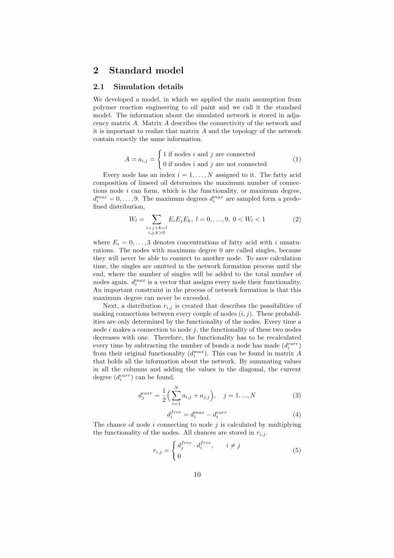
Every node has an index i = 1, . . . , N assigned to it. The fatty acidcomposition of linseed oil determines the maximum number of connec-tions node i can form, which is the functionality, or maximum degree,dmaxi = 0, . . . , 9. The maximum degrees dmaxi are sampled form a prede-fined distribution,

Wl =∑

i+j+k=li,j,k>0

EiEjEk, l = 0, . . . , 9, 0 < Wl < 1 (2)

where Ei = 0, . . . , 3 denotes concentrations of fatty acid with i unsatu-rations. The nodes with maximum degree 0 are called singles, becausethey will never be able to connect to another node. To save calculationtime, the singles are omitted in the network formation process until theend, where the number of singles will be added to the total number ofnodes again. dmaxi is a vector that assigns every node their functionality.An important constraint in the process of network formation is that thismaximum degree can never be exceeded.

Next, a distribution ri,j is created that describes the possibilities ofmaking connections between every couple of nodes (i, j). These probabil-ities are only determined by the functionality of the nodes. Every time anode i makes a connection to node j, the functionality of these two nodesdecreases with one. Therefore, the functionality has to be recalculatedevery time by subtracting the number of bonds a node has made (dcurri )from their original functionality (dmaxi ). This can be found in matrix Athat holds all the information about the network. By summating valuesin all the columns and adding the values in the diagonal, the currentdegree (dcurri ) can be found.

dcurrj =1

2

( N∑i=1

ai,j + aj,j

), j = 1, ..., N (3)

dfreei = dmaxi − dcurri (4)

The chance of node i connecting to node j is calculated by multiplyingthe functionality of the nodes. All chances are stored in ri,j .

ri,j =

{dfreej · dfreei , i 6= j

0(5)

10

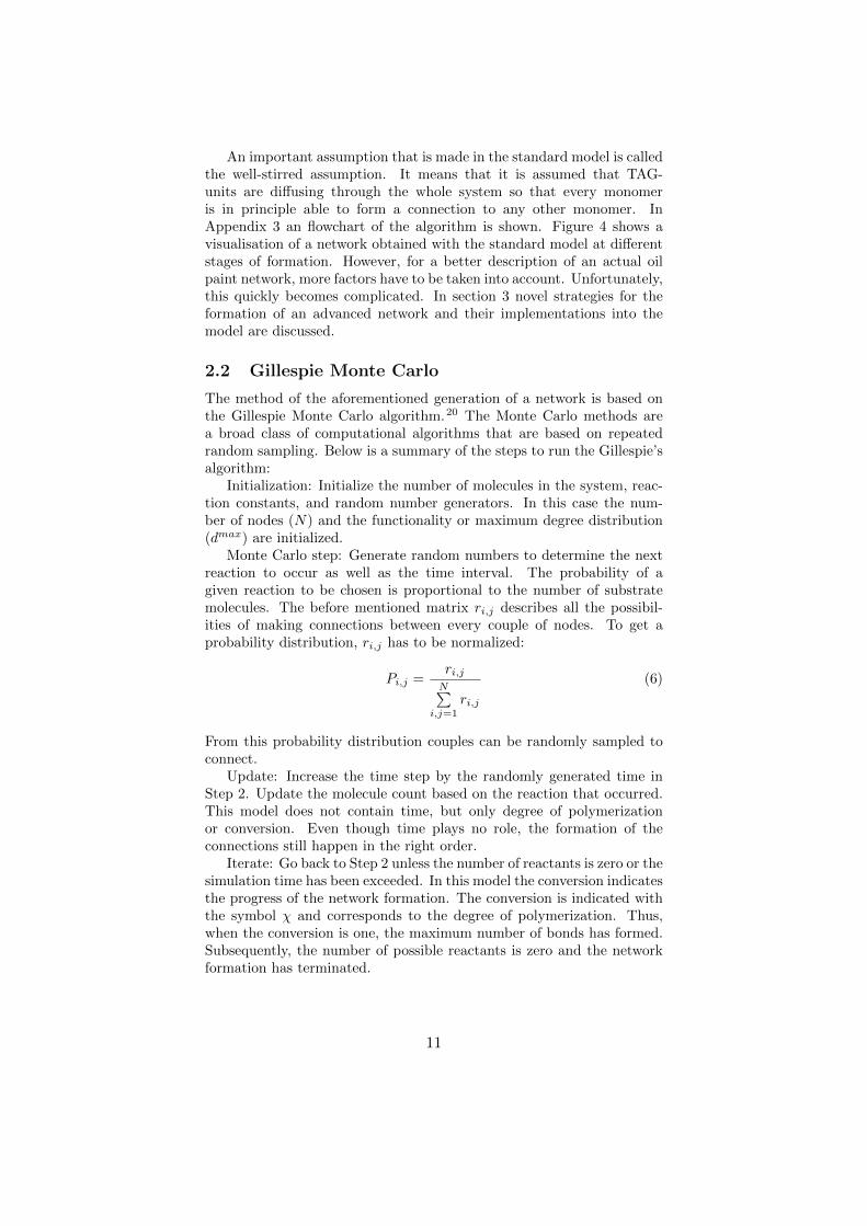
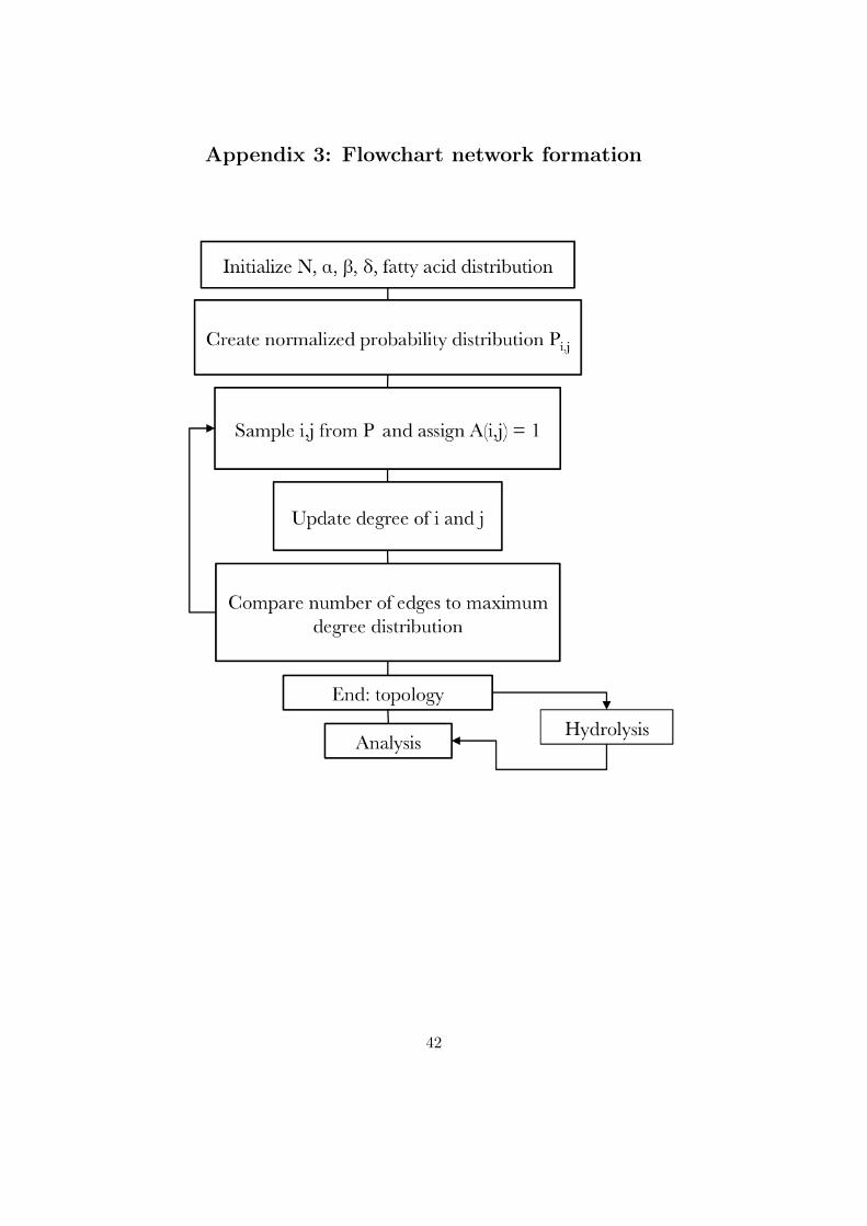
An important assumption that is made in the standard model is calledthe well-stirred assumption. It means that it is assumed that TAG-units are diffusing through the whole system so that every monomeris in principle able to form a connection to any other monomer. InAppendix 3 an flowchart of the algorithm is shown. Figure 4 shows avisualisation of a network obtained with the standard model at differentstages of formation. However, for a better description of an actual oilpaint network, more factors have to be taken into account. Unfortunately,this quickly becomes complicated. In section 3 novel strategies for theformation of an advanced network and their implementations into themodel are discussed.

2.2 Gillespie Monte Carlo

The method of the aforementioned generation of a network is based onthe Gillespie Monte Carlo algorithm.20 The Monte Carlo methods area broad class of computational algorithms that are based on repeatedrandom sampling. Below is a summary of the steps to run the Gillespie’salgorithm:

Initialization: Initialize the number of molecules in the system, reac-tion constants, and random number generators. In this case the num-ber of nodes (N) and the functionality or maximum degree distribution(dmax) are initialized.

Monte Carlo step: Generate random numbers to determine the nextreaction to occur as well as the time interval. The probability of agiven reaction to be chosen is proportional to the number of substratemolecules. The before mentioned matrix ri,j describes all the possibil-ities of making connections between every couple of nodes. To get aprobability distribution, ri,j has to be normalized:

Pi,j =ri,jN∑

i,j=1

ri,j

(6)

From this probability distribution couples can be randomly sampled toconnect.

Update: Increase the time step by the randomly generated time inStep 2. Update the molecule count based on the reaction that occurred.This model does not contain time, but only degree of polymerizationor conversion. Even though time plays no role, the formation of theconnections still happen in the right order.

Iterate: Go back to Step 2 unless the number of reactants is zero or thesimulation time has been exceeded. In this model the conversion indicatesthe progress of the network formation. The conversion is indicated withthe symbol χ and corresponds to the degree of polymerization. Thus,when the conversion is one, the maximum number of bonds has formed.Subsequently, the number of possible reactants is zero and the networkformation has terminated.

11

(a) χ = 0.16 (b) χ = 0.18

(c) χ = 0.23 (d) χ = 0.36

Figure 4: Visualisation of networks at different values of conversions (χ). The colors indicateindividual molecules, also called components, but have no further meaning.

12

2.3 Post-processing

The next step in this research is to analyze the generated network. Thereare several methods to post-process the data and they result in differentinteresting properties. In order to have as little fluctuations as possible,we generate a large number of networks with the same settings and av-erage these networks. This number varies from around 10 to a couplethousands. It depends on the property, because some are more sensitiveto fluctuations than others.

2.3.1 Component size distribution

The network consists of independent groups of connected nodes, calledcomponents (c). From a chemical point of view, these components aremolecules. Single nodes are components with size 1. The largest compo-nent is also called the giant component (cmax). To find the componentsof a network, a breadth-first search is executed.21 This is a standard al-gorithm that goes over all undiscovered nodes and finds their neighbours.With this information, the distribution of the nodes over the componentscan be found.

2.3.2 Gel fraction

Before the gel fraction can be discussed, first two very important concepts(sol and gel) have to be explained. During the drying process of oil paint,or the network formation, monomers start to connect and they form smallmolecules. While this happens, the system is still in the liquid phase,or the so-called sol regime. At some point, the giant molecule reachesa critical size and it becomes likely that it will consume all the othermolecules until all monomers are connected to each other. This point iscalled the gel point and the system after this point is in the solid phase,or gel regime. The gel fraction is the fraction of nodes involved in thegel.

2.3.3 Gel point

The gel point marks the transition from sol to gel. Experimentally, thegel point is visible as a jump in viscosity.22 To find the gel point inthis model, two networks are generated for two values of N and thesize of the giant component and of the second largest component arecalculated. When N is increased before gel point, the ratio between thegiant component and the second largest component stays the same orgoes down. This is because both these components are not part of thegel and grow independently from each other with a increasing number ofnodes. However, once the giant component starts to grow faster than thesecond largest component when N is increased, a gel is formed and thegel point is reached. Therefore, by looking at the ratio between the sizeof the giant component and the second largest component, the gel pointcan be identified.

13

2.3.4 Degree distribution

The degree distribution shows the degree of the nodes, which correspondsto their number of neighbours. This value can be calculated by summat-ing the ones in each column of matrix A as is shown in equation 3.

2.3.5 Cyclomatic number

The cyclomatic number G corresponds to the number of independentloops in the network. It is calculated by looking at the number of edges(m), number of nodes (N), and the number of disconnected components(molecules) M.

G = m−N +M (7)

Another way to interpret this number is as the maximum numberof edges that can be removed before the network does not contain anycycles, or in other words, before it becomes a tree network. If one edge ina tree network is removed, the network falls apart and is not connectedanymore. Therefore, the cyclomatic number can be used as a measurefor the resilience or strength of the network.

2.3.6 Average shortest path

The minimum number of edges between all the combinations of nodes iscalled the average shortest path and it is calculated using the Dijkstraalgorithm,23 which finds the shortest path between an initial node to acertain node Y . The average value of the shortest paths between all thenodes is a measure of the connectivity of the network. If the networkis heavily connected, by all sorts of cycles, the average shortest pathincreases, since it is not possible anymore to get from one side of thenetwork to the other in a few steps. The average shortest path can alsobe seen as a measure for the radius of a network.

2.3.7 Clustering coefficient

The clustering coefficient is the number of triangles connected to one nodedivided by the maximum number of possible triangles in the network. Anexample is shown in figure 5.

14

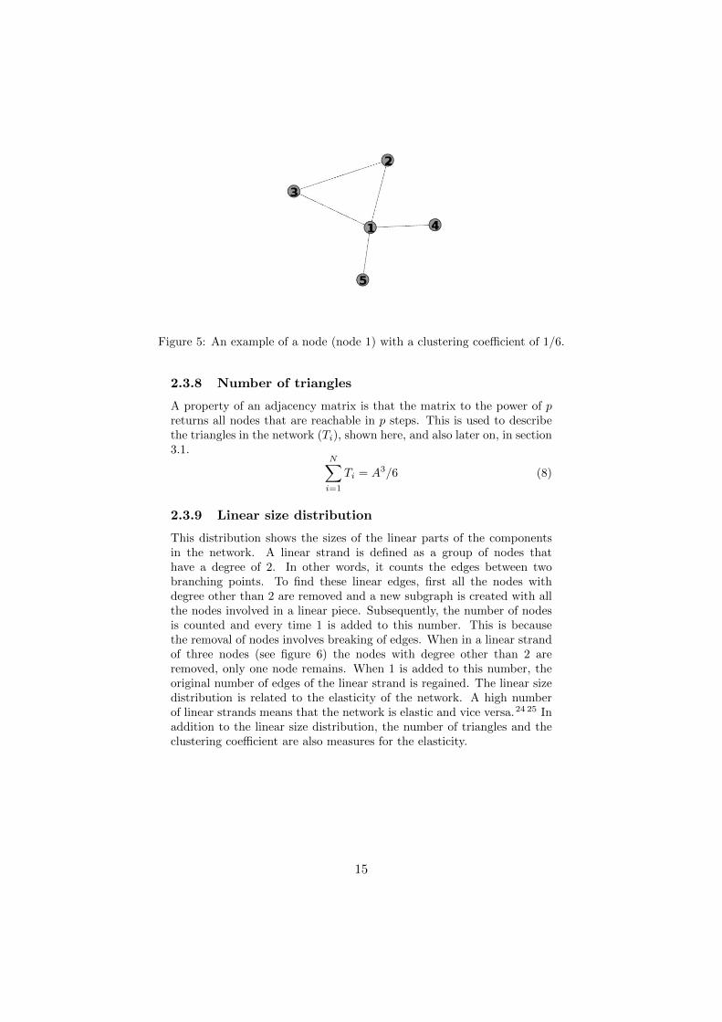
Figure 5: An example of a node (node 1) with a clustering coefficient of 1/6.

2.3.8 Number of triangles

A property of an adjacency matrix is that the matrix to the power of preturns all nodes that are reachable in p steps. This is used to describethe triangles in the network (Ti), shown here, and also later on, in section3.1.

N∑i=1

Ti = A3/6 (8)

2.3.9 Linear size distribution

This distribution shows the sizes of the linear parts of the componentsin the network. A linear strand is defined as a group of nodes thathave a degree of 2. In other words, it counts the edges between twobranching points. To find these linear edges, first all the nodes withdegree other than 2 are removed and a new subgraph is created with allthe nodes involved in a linear piece. Subsequently, the number of nodesis counted and every time 1 is added to this number. This is becausethe removal of nodes involves breaking of edges. When in a linear strandof three nodes (see figure 6) the nodes with degree other than 2 areremoved, only one node remains. When 1 is added to this number, theoriginal number of edges of the linear strand is regained. The linear sizedistribution is related to the elasticity of the network. A high numberof linear strands means that the network is elastic and vice versa.24 25 Inaddition to the linear size distribution, the number of triangles and theclustering coefficient are also measures for the elasticity.

15

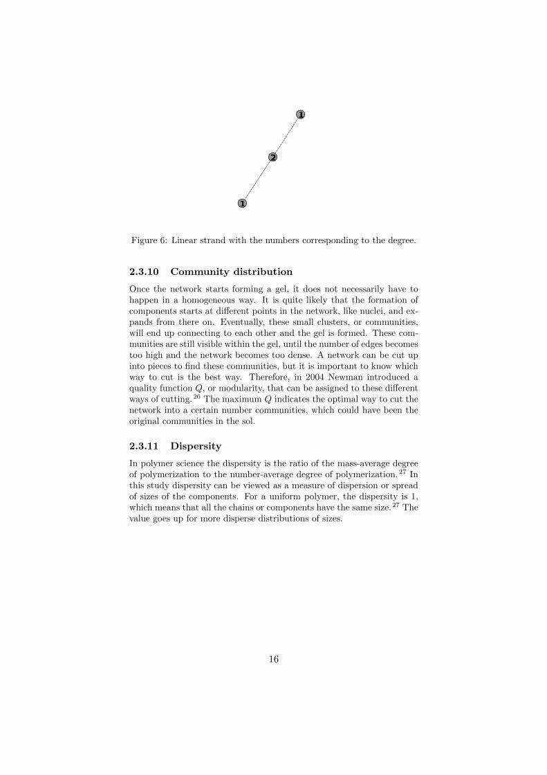
Figure 6: Linear strand with the numbers corresponding to the degree.

2.3.10 Community distribution

Once the network starts forming a gel, it does not necessarily have tohappen in a homogeneous way. It is quite likely that the formation ofcomponents starts at different points in the network, like nuclei, and ex-pands from there on. Eventually, these small clusters, or communities,will end up connecting to each other and the gel is formed. These com-munities are still visible within the gel, until the number of edges becomestoo high and the network becomes too dense. A network can be cut upinto pieces to find these communities, but it is important to know whichway to cut is the best way. Therefore, in 2004 Newman introduced aquality function Q, or modularity, that can be assigned to these differentways of cutting.26 The maximum Q indicates the optimal way to cut thenetwork into a certain number communities, which could have been theoriginal communities in the sol.

2.3.11 Dispersity

In polymer science the dispersity is the ratio of the mass-average degreeof polymerization to the number-average degree of polymerization.27 Inthis study dispersity can be viewed as a measure of dispersion or spreadof sizes of the components. For a uniform polymer, the dispersity is 1,which means that all the chains or components have the same size.27 Thevalue goes up for more disperse distributions of sizes.

16

2.4 Discussion of the results

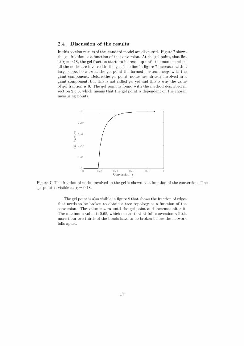
In this section results of the standard model are discussed. Figure 7 showsthe gel fraction as a function of the conversion. At the gel point, that liesat χ = 0.18, the gel fraction starts to increase up until the moment whenall the nodes are involved in the gel. The line in figure 7 increases with alarge slope, because at the gel point the formed clusters merge with thegiant component. Before the gel point, nodes are already involved in agiant component, but this is not called gel yet and this is why the valueof gel fraction is 0. The gel point is found with the method described insection 2.3.3, which means that the gel point is dependent on the chosenmeasuring points.

Conversion, χ0 0.2 0.4 0.6 0.8 1

Gel

fraction

0

0.2

0.4

0.6

0.8

1

Figure 7: The fraction of nodes involved in the gel is shown as a function of the conversion. Thegel point is visible at χ = 0.18.

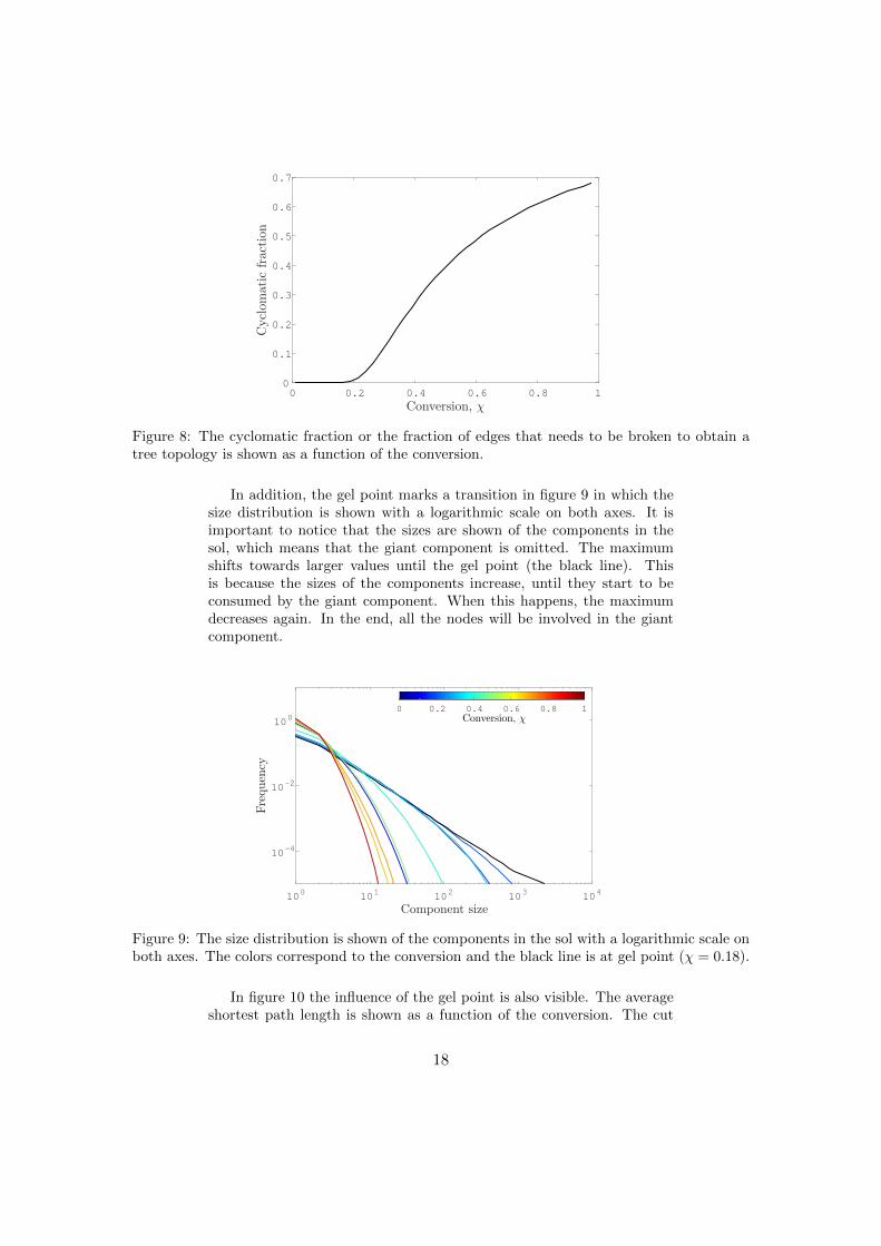
The gel point is also visible in figure 8 that shows the fraction of edgesthat needs to be broken to obtain a tree topology as a function of theconversion. The value is zero until the gel point and increases after it.The maximum value is 0.68, which means that at full conversion a littlemore than two thirds of the bonds have to be broken before the networkfalls apart.

17

Conversion, χ0 0.2 0.4 0.6 0.8 1

Cyclomaticfraction

0

0.1

0.2

0.3

0.4

0.5

0.6

0.7

Figure 8: The cyclomatic fraction or the fraction of edges that needs to be broken to obtain atree topology is shown as a function of the conversion.

In addition, the gel point marks a transition in figure 9 in which thesize distribution is shown with a logarithmic scale on both axes. It isimportant to notice that the sizes are shown of the components in thesol, which means that the giant component is omitted. The maximumshifts towards larger values until the gel point (the black line). Thisis because the sizes of the components increase, until they start to beconsumed by the giant component. When this happens, the maximumdecreases again. In the end, all the nodes will be involved in the giantcomponent.

Component size10

010

110

210

310

4

Frequen

cy

10-4

10-2

100

0 0.2 0.4 0.6 0.8 1

Conversion, χ

Figure 9: The size distribution is shown of the components in the sol with a logarithmic scale onboth axes. The colors correspond to the conversion and the black line is at gel point (χ = 0.18).

In figure 10 the influence of the gel point is also visible. The averageshortest path length is shown as a function of the conversion. The cut

18

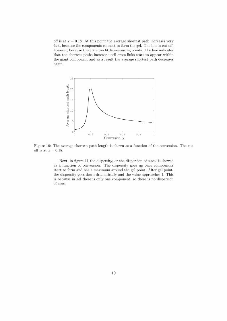
off is at χ = 0.18. At this point the average shortest path increases veryfast, because the components connect to form the gel. The line is cut off,however, because there are too little measuring points. The line indicatesthat the shortest paths increase until cross-links start to appear withinthe giant component and as a result the average shortest path decreasesagain.

Conversion, χ0 0.2 0.4 0.6 0.8 1

Averageshortestpath

length

0

5

10

15

20

25

Figure 10: The average shortest path length is shown as a function of the conversion. The cutoff is at χ = 0.18.

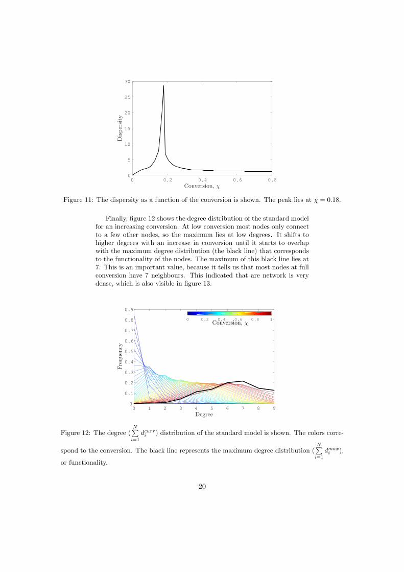
Next, in figure 11 the dispersity, or the dispersion of sizes, is showedas a function of conversion. The dispersity goes up once componentsstart to form and has a maximum around the gel point. After gel point,the dispersity goes down dramatically and the value approaches 1. Thisis because in gel there is only one component, so there is no dispersionof sizes.

19

Conversion, χ0 0.2 0.4 0.6 0.8

Dispersity

0

5

10

15

20

25

30

Figure 11: The dispersity as a function of the conversion is shown. The peak lies at χ = 0.18.

Finally, figure 12 shows the degree distribution of the standard modelfor an increasing conversion. At low conversion most nodes only connectto a few other nodes, so the maximum lies at low degrees. It shifts tohigher degrees with an increase in conversion until it starts to overlapwith the maximum degree distribution (the black line) that correspondsto the functionality of the nodes. The maximum of this black line lies at7. This is an important value, because it tells us that most nodes at fullconversion have 7 neighbours. This indicated that are network is verydense, which is also visible in figure 13.

Degree0 1 2 3 4 5 6 7 8 9

Frequency

0

0.1

0.2

0.3

0.4

0.5

0.6

0.7

0.8

0.9

0 0.2 0.4 0.6 0.8 1

Conversion, χ

Figure 12: The degree (N∑i=1

dcurri ) distribution of the standard model is shown. The colors corre-

spond to the conversion. The black line represents the maximum degree distribution (N∑i=1

dmaxi ),

or functionality.

20

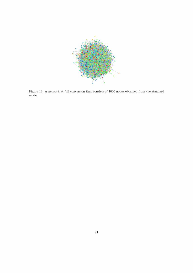
Figure 13: A network at full conversion that consists of 1000 nodes obtained from the standardmodel.

21

3 Advanced network formation

The standard model is based on a simple principle and it results in a verydense network. Whether this network is too dense and therefore unphysi-cal, will be discussed later on in this section. First, the implementation ofthree factors, intramolecular bonds, preferential coupling and shielding,are discussed. We modified the standard model and included these threefactor so that will make the model approach a realistic chemical systemmore accurately and we call this modified model the advanced model.

3.1 Preferential coupling

An important factor in the formation of the network is called preferentialcoupling. In a real chemical network nodes are not randomly connected,but certain couples are preferred. Preferential coupling indicates theinfluence of the topology of the network. The definition is simple: whentwo nodes are close to each other, they are more likely to connect. Theimplementation, however, is not as simple. This is because position is notspecified in this model. Therefore, we have to look at the connections thatthe nodes have already formed. The probability of two nodes that arelinked through a common neighbour is increased and this effect decreaseswhen the path between the two nodes becomes longer. To find the nodesthat are connected by a path of length p, it is enough to consider thepth power of the adjacency matrix. Indeed, an i, j-element of matrix Ap

equals to 0 unless there exists a link between nodes i, j of length p. Inthis operation, however, the edges can be counted more than one timeand this is not desired. Here we will define a matrix Ap. An i, j-elementof this matrix is equal to 0 if the nodes are connected by a link of lengthp but are not connected with a shorter link:

Ap = (Ap > 0) · (1−Ap−1) (9)

Here (Ap > 0)i,j is 1 if i, j-element of Ap is greater than 0, and operation”·” should be understood as the element-wise multiplication.

The distribution ri,j , obtained from the standard model, is modifiedby multiplying it with a certain factor. In this factor, matrix Ap is mul-tiplied with path length p with a certain exponent. This exponent p−3/2

indicates that probability for connecting two nodes decays algebraicallyas topological distance p increases.14 The parameter α determines thestrength of the influence of the preferential coupling. Equation 11 showsthe normalization step.

r′i,j = ri,j · (1 + α

pmax∑p=1

App−3/2) (10)

Pi,j =r′i,jN∑

i,j=1

r′i,j

(11)

Also, more than one bond between the nodes is allowed. The function-ality of the nodes is updated every time a connection is formed. When

22

a couple is sampled that already made a connection, the 1 in matrix Astays unchanged, but the functionality of these nodes decreases. There-fore, matrix A is still only filled with zeroes and ones.

3.1.1 Discussion of the results

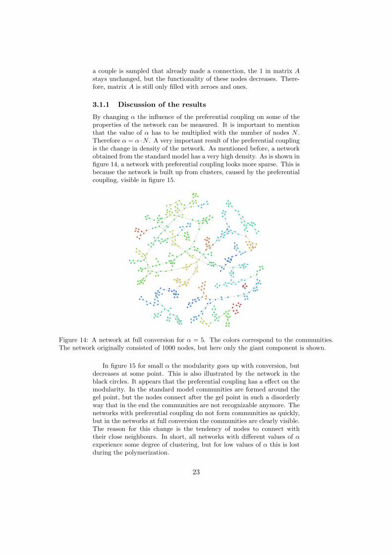
By changing α the influence of the preferential coupling on some of theproperties of the network can be measured. It is important to mentionthat the value of α has to be multiplied with the number of nodes N .Therefore α = α ·N . A very important result of the preferential couplingis the change in density of the network. As mentioned before, a networkobtained from the standard model has a very high density. As is shown infigure 14, a network with preferential coupling looks more sparse. This isbecause the network is built up from clusters, caused by the preferentialcoupling, visible in figure 15.

Figure 14: A network at full conversion for α = 5. The colors correspond to the communities.The network originally consisted of 1000 nodes, but here only the giant component is shown.

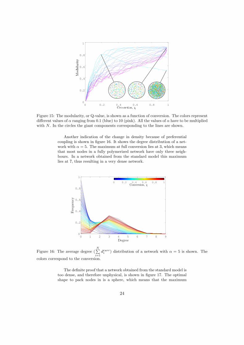
In figure 15 for small α the modularity goes up with conversion, butdecreases at some point. This is also illustrated by the network in theblack circles. It appears that the preferential coupling has a effect on themodularity. In the standard model communities are formed around thegel point, but the nodes connect after the gel point in such a disorderlyway that in the end the communities are not recognizable anymore. Thenetworks with preferential coupling do not form communities as quickly,but in the networks at full conversion the communities are clearly visible.The reason for this change is the tendency of nodes to connect withtheir close neighbours. In short, all networks with different values of αexperience some degree of clustering, but for low values of α this is lostduring the polymerization.

23

0 0.2 0.4 0.6 0.8 10

0.2

0.4

0.6

0.8

1

Figure 15: The modularity, or Q-value, is shown as a function of conversion. The colors representdifferent values of α ranging from 0.1 (blue) to 10 (pink). All the values of α have to be multipliedwith N . In the circles the giant components corresponding to the lines are shown.

Another indication of the change in density because of preferentialcoupling is shown in figure 16. It shows the degree distribution of a net-work with α = 5. The maximum at full conversion lies at 3, which meansthat most nodes in a fully polymerized network have only three neigh-bours. In a network obtained from the standard model this maximumlies at 7, thus resulting in a very dense network.

Degree0 1 2 3 4 5 6 7 8 9

Frequency

0

0.2

0.4

0.6

0.8

1

0 0.2 0.4 0.6 0.8 1

Conversion, χ

Figure 16: The average degree (N∑i=1

dcurri ) distribution of a network with α = 5 is shown. The

colors correspond to the conversion.

The definite proof that a network obtained from the standard model istoo dense, and therefore unphysical, is shown in figure 17. The optimalshape to pack nodes in is a sphere, which means that the maximum

24

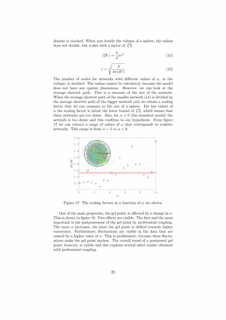
density is reached. When you double the volume of a sphere, the radiusdoes not double, but scales with a factor of 3

√2:

(2V ) =4

3πr3 (12)

r = 3

√3

4π(2V )(13)

The number of nodes for networks with different values of α, or thevolume, is doubled. The radius cannot be calculated, because the modeldoes not have any spatial dimensions. However, we can look at theaverage shortest path. This is a measure of the size of the network.When the average shortest path of the smaller network (a1) is divided bythe average shortest path of the bigger network (a2) we obtain a scalingfactor that we can compare to the one of a sphere. For low values ofα the scaling factor is below the lower bound of 3

√2, which means that

these networks are too dense. Also, for α = 0 (the standard model) thenetwork is too dense and this confirms to our hypothesis. From figure17 we can extract a range of values of α that corresponds to realisticnetworks. This range is from α = 5 to α = 8.

Figure 17: The scaling factors as a function of α are shown.

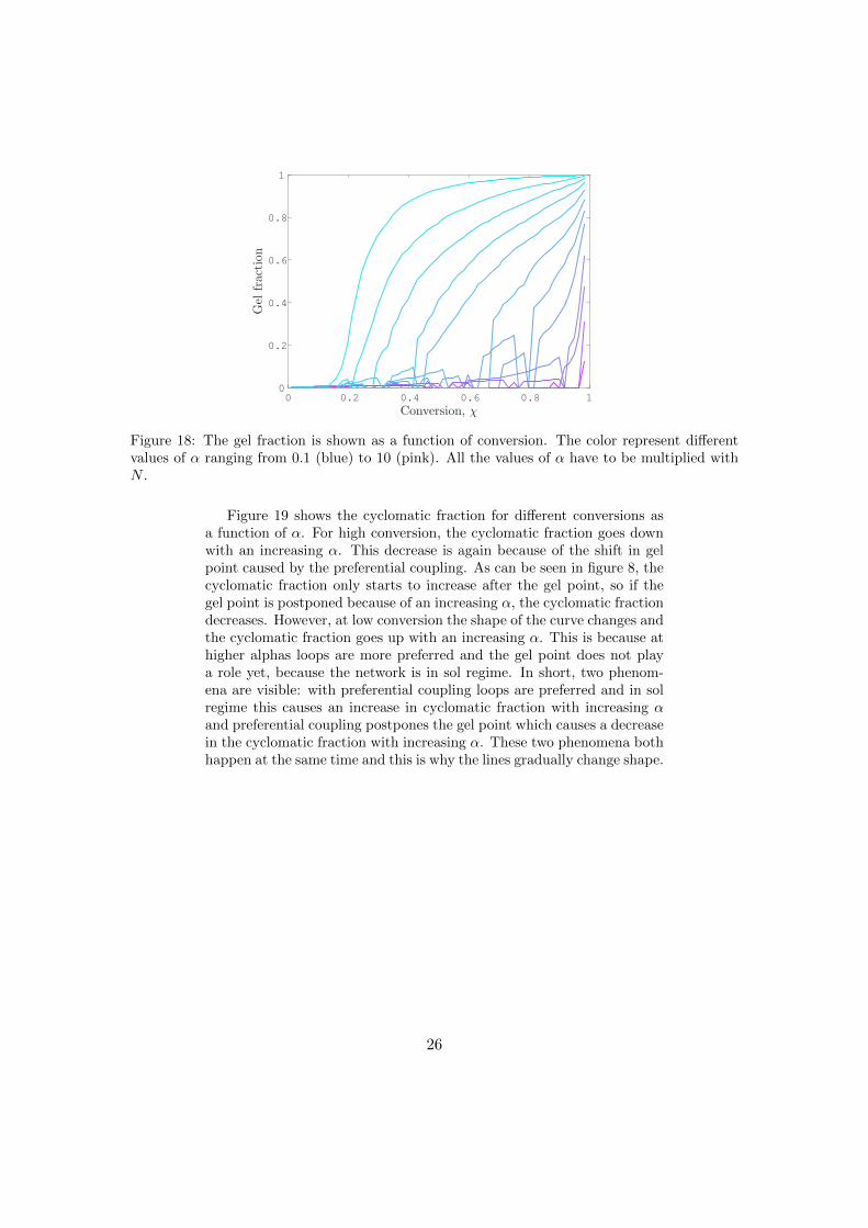
One of the main properties, the gel point, is affected by a change in α.This is shown in figure 18. Two effects are visible. The first and the mostimportant is the postponement of the gel point by preferential coupling.The more α increases, the more the gel point is shifted towards higherconversion. Furthermore, fluctuations are visible in the data that arecaused by a higher value of α. This is problematic, because these fluctu-ations make the gel point unclear. The overall trend of a postponed gelpoint, however, is visible and this explains several other results obtainedwith preferential coupling.

25

Conversion, χ0 0.2 0.4 0.6 0.8 1

Gel

fraction

0

0.2

0.4

0.6

0.8

1

Figure 18: The gel fraction is shown as a function of conversion. The color represent differentvalues of α ranging from 0.1 (blue) to 10 (pink). All the values of α have to be multiplied withN .

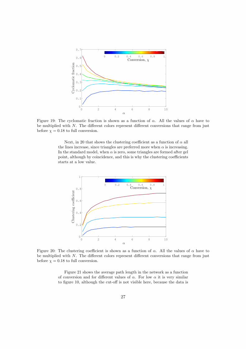
Figure 19 shows the cyclomatic fraction for different conversions asa function of α. For high conversion, the cyclomatic fraction goes downwith an increasing α. This decrease is again because of the shift in gelpoint caused by the preferential coupling. As can be seen in figure 8, thecyclomatic fraction only starts to increase after the gel point, so if thegel point is postponed because of an increasing α, the cyclomatic fractiondecreases. However, at low conversion the shape of the curve changes andthe cyclomatic fraction goes up with an increasing α. This is because athigher alphas loops are more preferred and the gel point does not playa role yet, because the network is in sol regime. In short, two phenom-ena are visible: with preferential coupling loops are preferred and in solregime this causes an increase in cyclomatic fraction with increasing αand preferential coupling postpones the gel point which causes a decreasein the cyclomatic fraction with increasing α. These two phenomena bothhappen at the same time and this is why the lines gradually change shape.

26

α

0 2 4 6 8 10

Cyclomaticfraction

0

0.1

0.2

0.3

0.4

0.5

0.6

0.7

0 0.2 0.4 0.6 0.8 1

Conversion, χ

Figure 19: The cyclomatic fraction is shown as a function of α. All the values of α have tobe multiplied with N . The different colors represent different conversions that range from justbefore χ = 0.18 to full conversion.

Next, in 20 that shows the clustering coefficient as a function of α allthe lines increase, since triangles are preferred more when α is increasing.In the standard model, when α is zero, some triangles are formed after gelpoint, although by coincidence, and this is why the clustering coefficientsstarts at a low value.

α

0 2 4 6 8 10

Clusteringcoeffi

cient

0

0.2

0.4

0.6

0.8

1

0 0.2 0.4 0.6 0.8 1

Conversion, χ

Figure 20: The clustering coefficient is shown as a function of α. All the values of α have tobe multiplied with N . The different colors represent different conversions that range from justbefore χ = 0.18 to full conversion.

Figure 21 shows the average path length in the network as a functionof conversion and for different values of α. For low α it is very similarto figure 10, although the cut-off is not visible here, because the data is

27

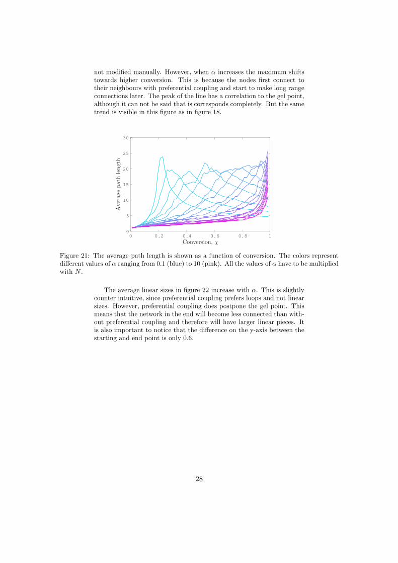
not modified manually. However, when α increases the maximum shiftstowards higher conversion. This is because the nodes first connect totheir neighbours with preferential coupling and start to make long rangeconnections later. The peak of the line has a correlation to the gel point,although it can not be said that is corresponds completely. But the sametrend is visible in this figure as in figure 18.

Conversion, χ0 0.2 0.4 0.6 0.8 1

Averagepath

length

0

5

10

15

20

25

30

Figure 21: The average path length is shown as a function of conversion. The colors representdifferent values of α ranging from 0.1 (blue) to 10 (pink). All the values of α have to be multipliedwith N .

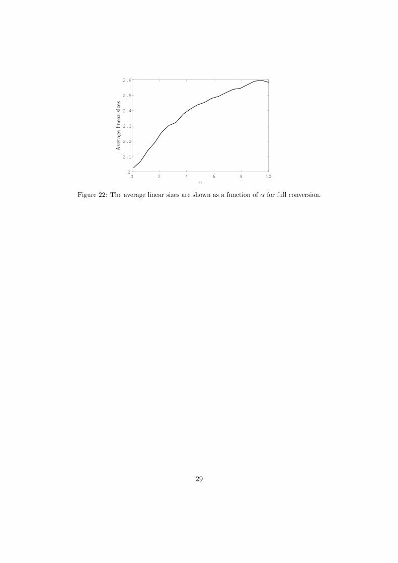
The average linear sizes in figure 22 increase with α. This is slightlycounter intuitive, since preferential coupling prefers loops and not linearsizes. However, preferential coupling does postpone the gel point. Thismeans that the network in the end will become less connected than with-out preferential coupling and therefore will have larger linear pieces. Itis also important to notice that the difference on the y-axis between thestarting and end point is only 0.6.

28

α

0 2 4 6 8 10

Averagelinearsizes

2

2.1

2.2

2.3

2.4

2.5

2.6

Figure 22: The average linear sizes are shown as a function of α for full conversion.

29

3.2 Intramolecular bonds

Another factor that influences the distribution ri,j is the formation of in-tramolecular bonds. Intramolecular bonds are cross-links formed betweenfatty acids within the same TAG-unit. In matrix A this is represented bya one on the diagonal. The chance of a node forming a connection withitself is a certain constant β times a binomial coefficient that indicates allthe possible intramolecular bonds. The binomial coefficient

(nk

)tells you

how many groups of size k can be formed from n things. To make surethat the intramolecular bonds are only made between the different fattyacids in a TAG-unit, and not within the same fatty acid, the binomialcoefficient is not based on the functionality of the node. The trick is tolook at the individual fatty acids in the TAG-units (dfai ) and take for then of the binomial coefficient the functionality of each fatty acid in oneTAG-unit and for k 2. This is added on the diagonal of matrix ri,j . Toget probability distribution Pi,j , ri,j has be normalized.

ri,j =

(dfreej ) · (dfreei ), i 6= j

β

(dfai2

), i = j

(14)

An important step in the intramolecular bonds is the update step.Once an intramolecular bonds has formed, the functionality of the fattyacids within the TAG-unit has to be updated. This is executed as follows.An array is made that contains the functionality of the three fatty acidsper node. If a one is placed in the matrix at the diagonal at node i, thefunctionality of the fatty acids of this node will be updated. Two of thefatty acids from node i are sampled and the functionality of these fattyacids will be lowered with 1. Because normal connections also change thefunctionality of the fatty acids, this updating procedure is also appliedon normal bond formation between two nodes. In that case one of thefatty acids of node i is sampled and one of the fatty acids of node j and1 is subtracted from their functionality.

3.2.1 Discussion of the results

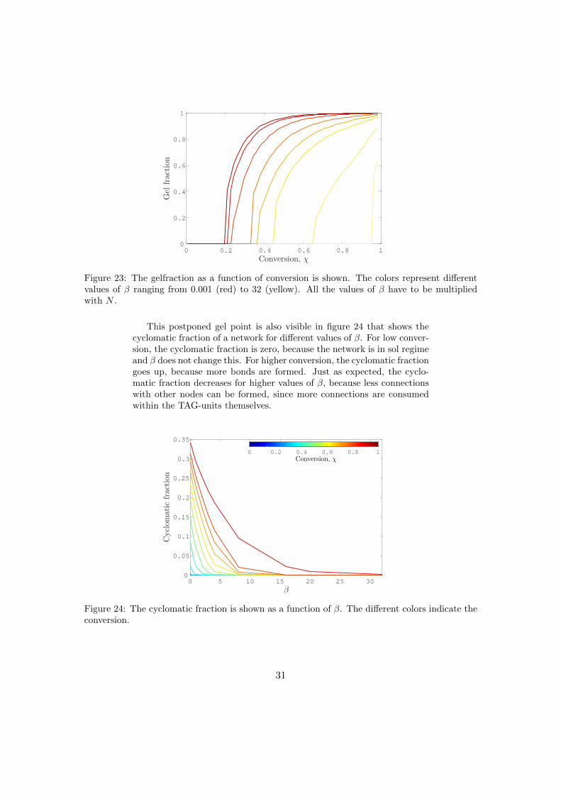
The influence of β on the gel point, shown in figure 23 is clear: it shiftsthe gel point towards higher conversion as expected. Thus, the formationof intramolecular bonds postpones the formation of a gel.

30

Conversion, χ0 0.2 0.4 0.6 0.8 1

Gel

fraction

0

0.2

0.4

0.6

0.8

1

Figure 23: The gelfraction as a function of conversion is shown. The colors represent differentvalues of β ranging from 0.001 (red) to 32 (yellow). All the values of β have to be multipliedwith N .

This postponed gel point is also visible in figure 24 that shows thecyclomatic fraction of a network for different values of β. For low conver-sion, the cyclomatic fraction is zero, because the network is in sol regimeand β does not change this. For higher conversion, the cyclomatic fractiongoes up, because more bonds are formed. Just as expected, the cyclo-matic fraction decreases for higher values of β, because less connectionswith other nodes can be formed, since more connections are consumedwithin the TAG-units themselves.

β0 5 10 15 20 25 30

Cyclomaticfraction

0

0.05

0.1

0.15

0.2

0.25

0.3

0.35

0 0.2 0.4 0.6 0.8 1

Conversion, χ

Figure 24: The cyclomatic fraction is shown as a function of β. The different colors indicate theconversion.

31

3.3 Shielding

Shielding or steric hindrance implies that if the surroundings of a nodeare too crowded, the probability of making a connection to another nodeis very low. At first, we developed a simple method to describe the shield-ing. Nodes that are involved in one or more triangles are defined as beingshielded and experience a negative effect on the probability of making anew connection. To calculate this effect, first the local triangles (Ti), orthe triangles each node is involved in, are calculated by multiplying theclustering coefficient by the number of possible triangles around everynode, which can be calculated by a binomial coefficient. In this case,n represents the number of edges connected to this node, or dcurr, andk is 2. The local clustering coefficient (Ci) is the number of trianglesaround a certain node divided by the possible triangles around this node(see section 2.3.7). Now, the effect (S) can be calculated and it shouldbe negative. This is why Ti is in the denominator multiplied by a cer-tain constant δ that determines the strength of the shielding effect. Theshielding effect Si is multiplied with ri,j .

Ti = Ci ·(dcurri

2

)(15)

Si =1

(Ti + 1)δ(16)

ri,j = Si · ri,j , i 6= j (17)

However, this description is too simple, because only triangles aretaken into account. A more elegant way to describe the shielding effectis with the use of an eigenvector. This method is based on the pageranking method that Google R© uses.28 The idea is that the shielding ofnode i depends on the number of neighbours j and on their shielding.But their shielding again depends on the number of neighbours and theirshielding, which includes the shielding of node i. This is comparable tothe eigenvalue problem of the ranking of page i, which is based on theranking of all the pages that link to page i. Also, this effect is tunedby parameter δ. In this report, no results of the influence of δ will bediscussed, because of time reasons.

32

4 Validation of the model

In order to use the results obtained from the model, some kind of vali-dation is necessary. Within the PAinT group an experiment is designedthat will form the link between the model and reality. The experimentis based on the hydrolysis of the TAG-units. As mentioned before, theproblem with obtaining structural information about the molecular topol-ogy of oil paint, is the high connectivity and complexity of the network.Only before the gel point, the structure of the loose components can beanalyzed. Therefore, the solution would be to do an experiment thatpostpones the gel point. This is exactly what happens when the networkis hydrolyzed. The ester bonds between the glycerol molecule and thefatty acids in the TAG-units are broken. However, the cross-links areretained and therefore, we obtain fragments that still have the originalcross-links. The fragments can be analyzed with GC-MS and a size dis-tribution can be measured. When this is compared to the simulated sizedistribution, the original network can be found through the model. Inthis section the algorithm that we developed to simulate this experimentis discussed.

1. Creating distribution array: for nodes i to N three degrees aresampled from the fatty acid distribution and these values are stored inan array, while it is made sure that the three values, a, b, and c, togetherdo not exceed the maximum degree, or functionality, of every node. Thisis done because the nodes will be split up into three pieces, a, b and c.

2. Sampling: for every node i its neighbours are found. For neighbourj piece a, b or c is sampled. If a is sampled, it means that neighbour jis connected to piece a of node i and nothing will change in matrix A.This is because after hydrolysis piece a will be seen as a new node.

3. Edge removal and creation of new node: When piece b or c issampled, it means that neighbour j is connected to piece b or c. Nowthis edge between node i and j is removed and a new node is created. Inother words, node i is divided into three parts and the degrees of thesethree parts together will be equal to the degree of the original node. It isimportant to take into account that matrix A has to stay symmetrical.Therefore, the actions described in equation 18 have to be executed aswell for A(i, j) as for laA(j, i), but when i = j only one edge has to beremoved.

if piece b is sampled A(i, j) = A(i, j)− 1, A(j, (n+ 1)) = 1if piece c is sampled A(i, j) = A(i, j)− 1, A(j, (n+ 2)) = 1

(18)

4. Iterate: this procedure is executed for nodes i, ..., N .In case of intramolecular bonds, the hydrolysis algorithm has to be

modified, because the TAG-unit will not be split up completely, whentwo fatty acids are connected via an intramolecular bond. This problemis solved by making a distribution of the probabilities of the possible

33

intramolecular bonds between the three fatty acids:

p1 = dcurrfa1 · dcurrfa2

p2 = dcurrfa2 · dcurrfa3

p3 = dcurrfa3 · dcurrfa1

(19)

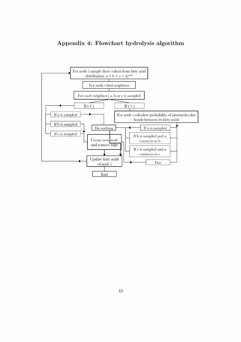
In step 2 not only a value from the first distribution array is sampled, butalso a value from the second distribution array (equation 19). Now forevery neighbour j of every node i it is known to which part of node i it isconnected and it is known which two fatty acids are connected inside nodei. If neighbour j connects to piece a or if it connects to piece b and thispiece is connected via intramolecular bonding to piece a or if it connectsto piece c and this piece is connected to piece a nothing will happen. Forthe other possibilities, a new node is created. This modified algorithmwill only hold as long as only one intramolecular bond is formed, whichis fixed in the network formation algorithm. To improve the model, morethan one intramolecular bond has to be allowed. However, the modeldescribed in this report does not allow more than one intramolecularbond.

if

a is sampled

b is sampled, b connects to a

c is sampled, c connects to a

continue

if else A(i, j) = A(i, j)− 1, A(j, (n+ 1)) = 1(20)

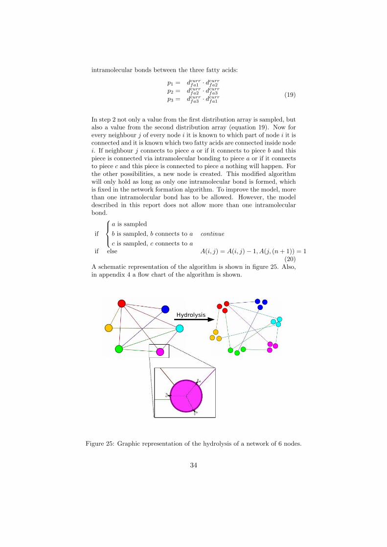
A schematic representation of the algorithm is shown in figure 25. Also,in appendix 4 a flow chart of the algorithm is shown.

Figure 25: Graphic representation of the hydrolysis of a network of 6 nodes.

34

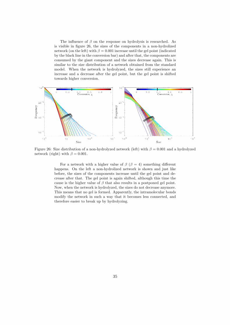
The influence of β on the response on hydrolysis is researched. Asis visible in figure 26, the sizes of the components in a non-hydrolizednetwork (on the left) with β = 0.001 increase until the gel point (indicatedby the black line in the conversion bar) and after that, the components areconsumed by the giant component and the sizes decrease again. This issimilar to the size distribution of a network obtained from the standardmodel. When the network is hydrolyzed, the sizes still experience anincrease and a decrease after the gel point, but the gel point is shiftedtowards higher conversion.

Figure 26: Size distribution of a non-hydrolyzed network (left) with β = 0.001 and a hydrolyzednetwork (right) with β = 0.001.

For a network with a higher value of β (β = 4) something differenthappens. On the left a non-hydrolized network is shown and just likebefore, the sizes of the components increase until the gel point and de-crease after that. The gel point is again shifted, although this time thecause is the higher value of β that also results in a postponed gel point.Now, when the network is hydrolyzed, the sizes do not decrease anymore.This means that no gel is formed. Apparently, the intramolecular bondsmodify the network in such a way that it becomes less connected, andtherefore easier to break up by hydrolyzing.

35

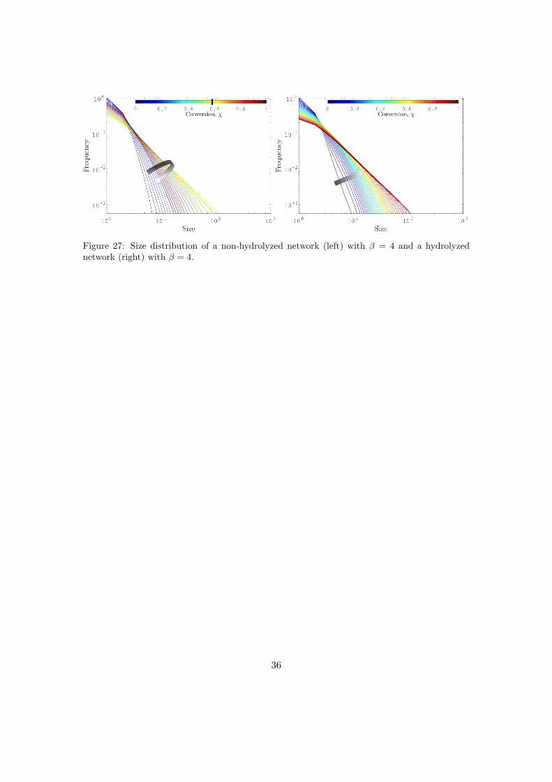
Figure 27: Size distribution of a non-hydrolyzed network (left) with β = 4 and a hydrolyzednetwork (right) with β = 4.

36

5 Conclusion

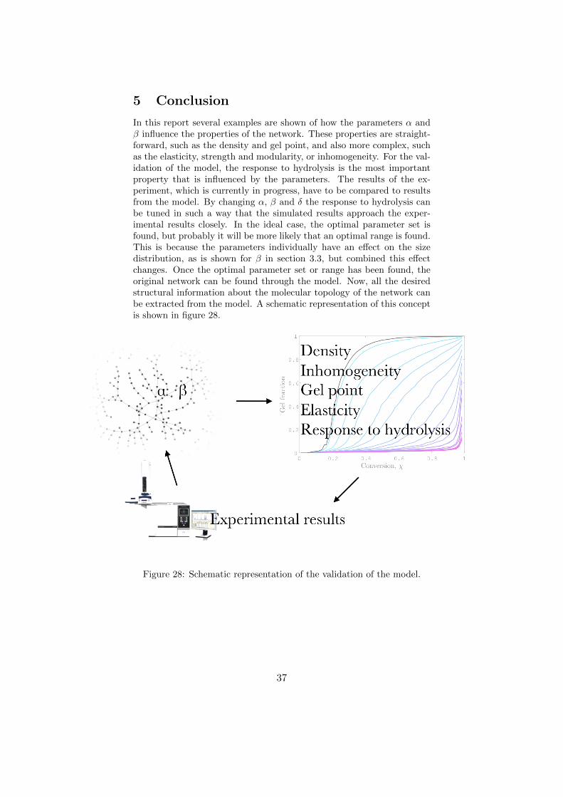
In this report several examples are shown of how the parameters α andβ influence the properties of the network. These properties are straight-forward, such as the density and gel point, and also more complex, suchas the elasticity, strength and modularity, or inhomogeneity. For the val-idation of the model, the response to hydrolysis is the most importantproperty that is influenced by the parameters. The results of the ex-periment, which is currently in progress, have to be compared to resultsfrom the model. By changing α, β and δ the response to hydrolysis canbe tuned in such a way that the simulated results approach the exper-imental results closely. In the ideal case, the optimal parameter set isfound, but probably it will be more likely that an optimal range is found.This is because the parameters individually have an effect on the sizedistribution, as is shown for β in section 3.3, but combined this effectchanges. Once the optimal parameter set or range has been found, theoriginal network can be found through the model. Now, all the desiredstructural information about the molecular topology of the network canbe extracted from the model. A schematic representation of this conceptis shown in figure 28.

Figure 28: Schematic representation of the validation of the model.

37

The model that we developed and that is discussed in this report is anew model that incorporates novel advanced routines. In the advancedmodel, the system is completely represented by the topology and it isalso the topology that defines the reactivity of the monomers, in stead ofonly the functionality. Because the system is represented by the topology,there is no space involved. But it is like a trade-off; because there are nospatial dimensions, it makes the model time and space scalable. Spacescalable means that it is applicable to other systems. The size of themonomers of other systems is not of importance, because they can stillbe represented as nodes. Time scalable means that paint alterations canbe studies with our model either in microseconds or in centuries.

Our model provides an important step towards understanding thephysical properties of oil paint and these insights will help to explain theinteraction of pigments with the network and the degradation processesin oil paintings; highly valuable knowledge for conservations scientists.Furthermore, not only oil paint, but also industrial polymer networkscan be studied using our model.

38

6 Prospects

In this report the development of a novel model and its first results arediscussed. Also, a start is made for the validation of the model. Inthe PAinT group, progress is being made in the design of the hydrolysisexperiment. It turns out that the full hydrolysis of the network is quitedifficult and also the solving of this hydrolyzed network. There are exper-iments running with loose fatty acids that are cured and analyzed. Thesehydrolysis experiments are promising and important for the validation ofthe model. It will be important to design the optimal experiment to findthe optimal range of parameters.

Also, more routines can be added to the advanced model, to simulate areal chemical system even more accurately. The problem is, however, thatmore unknown parameters need to be added. Therefore, it is importantconsider the necessity of these routines.

Finally, it will be interesting to investigate certain processes on asmaller scale with for example DFT calculations. Density FunctionalTheory (DFT) is a very accurate method to simulate chemical reactionson an atomic scale.29 To see whether for example pigments affect thepolymerization of the oil paint, DFT can be employed. The majorityof pigments are metal salts and their reactivity is an intensely studiedsubject within art research and the PAinT group.30 31 Results of thesecalculations could predict the value of parameters that can be added toour model.

7 Acknowledgments

I would like to thank my daily supervisor dr. Ivan Kryven (HIMS, UvA)for his help and support. I would also like to thank Prof. dr. PietIedema (HIMS, UvA) and dr. Celia Fonseca Guerra (Division of Theo-retical Chemistry, VU) for their supervision. Furthermore, I would liketo thank the Computational Chemistry Group at the UvA and the PaintAlterations in Time Group, a collaboration between the HIMS Instituteof the UvA and the Rijksmuseum. Lastly, I would like to acknowledgethe MIT Strategic Engineering Research Group for their on line databaseof Matlab R© tools for network analysis.

39

Appendix 1: Terminology

Community Group of nodes that is strongly connected to eachother and weakly connected to the rest of the gel

Component Independent group of connected nodesConnectivity Whether and how nodes are connected to one another

in the network18

Conversion Degree of polymerizationEdge Connection between two nodesDegree Current number of neighbours of a nodeFunctionality Maximum number of neighbours of a node, also called

maximum degreeGel Highly interconnected polymer network that is in solid

phaseGel point Transition point from sol to gel, also called percolation

thresholdGiant component The largest component in the networkGraph / Network Collection of nodes that is connected by edgesGraph theory The use of mathematical structures to describe con-

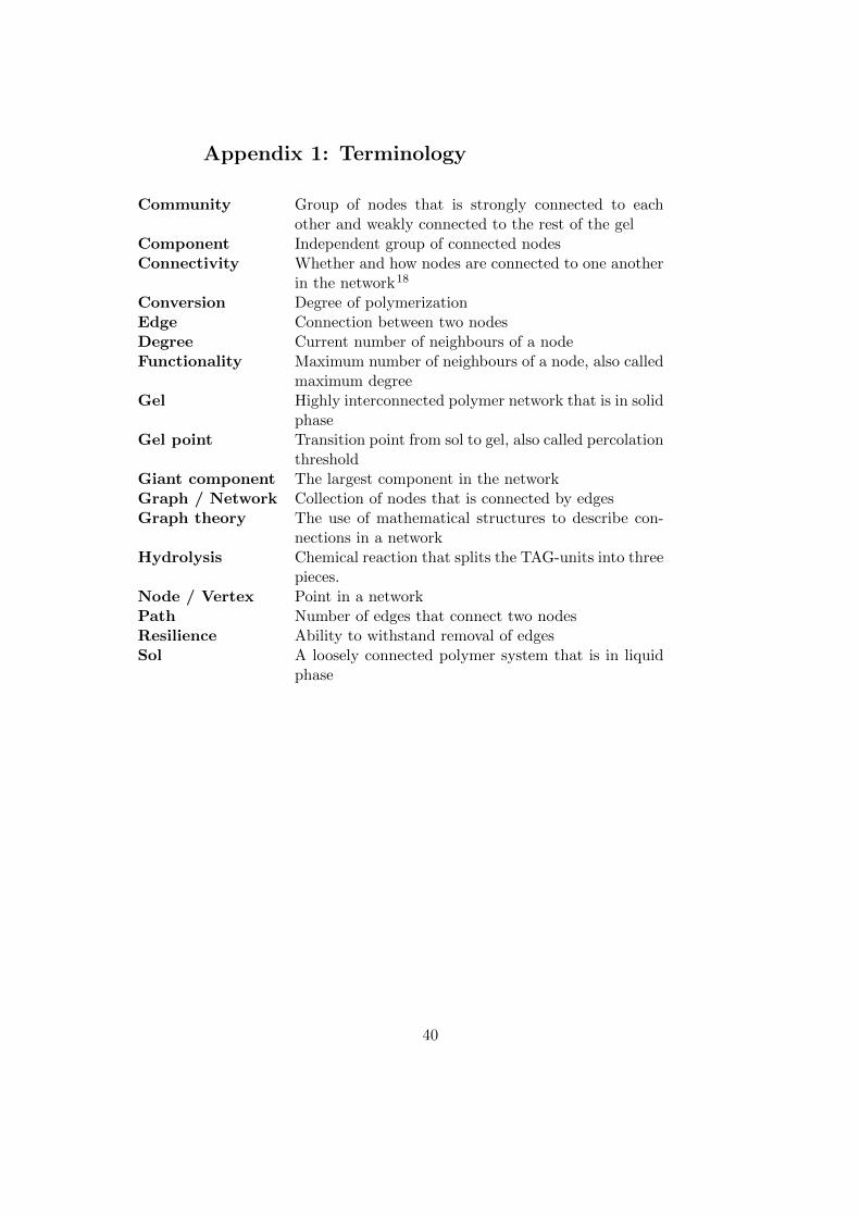
nections in a networkHydrolysis Chemical reaction that splits the TAG-units into three

pieces.Node / Vertex Point in a networkPath Number of edges that connect two nodesResilience Ability to withstand removal of edgesSol A loosely connected polymer system that is in liquid

phase

40

Appendix 2: Fatty acid composition

Fatty acid Chemical composition % in linseed oil

Palmitic acid C16:0 6,58%Stearic acid C18:0 4,43%Oleic acid C18:1 18,51%

Lineoleic acid C18:2 17,25%Linolenic aicd C18:3 53,21%

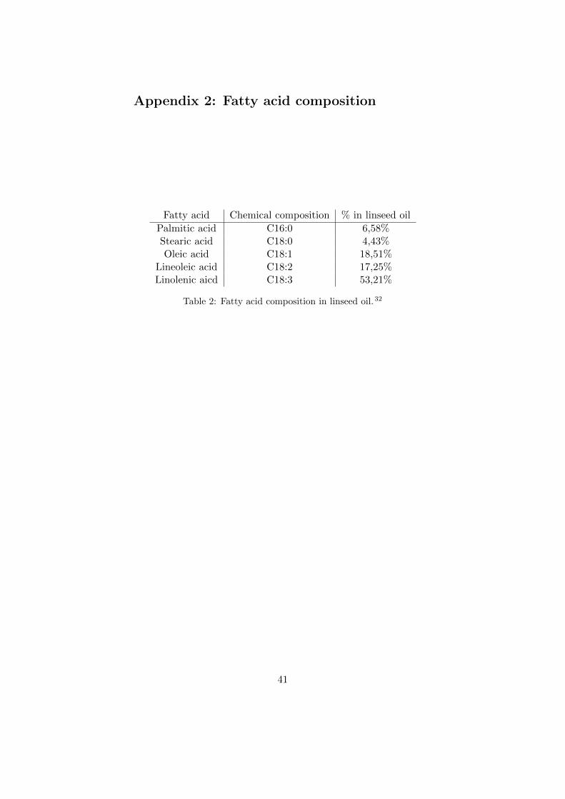
Table 2: Fatty acid composition in linseed oil.32

41

Appendix 3: Flowchart network formation

42

Appendix 4: Flowchart hydrolysis algorithm

43

References

[1] Janson, H. W.; Janson, A. F. History of art ; Harry N. Abrams NewYork, 2001.

[2] Van den Berg, J.; Van den Berg, K.; Boon, J. Determination of thedegree of hydrolysis of oil paint samples using a two-step derivatisa-tion method and on-column GC/MS. Progress in Organic Coatings2001, 41, 143–155.

[3] Soucek, M.; Khattab, T.; Wu, J. Review of autoxidation and driers.Progress in Organic Coatings 2012, 73, 435–454.

[4] Geldof, M. Finding the suspect of the discolouration of the floor,http://slaapkamergeheimen.vangoghmuseum.nl/category/collaboration/?lang=en(accessed June 20, 2015).

[5] Bonaduce, I.; Carlyle, L.; Colombini, M. P.; Duce, C.; Ferrari, C.;Ribechini, E.; Selleri, P.; Tine, M. R. New insights into the ageingof linseed oil paint binder: a qualitative and quantitative analyticalstudy. 2012,

[6] Van Gorkum, R.; Bouwman, E. The oxidative drying of alkydpaint catalysed by metal complexes. Coordination Chemistry Re-views 2005, 249, 1709–1728.

[7] Hamzehlou, S.; Reyes, Y.; Leiza, J. R. A new insight into the for-mation of polymer networks: a kinetic monte carlo simulation ofthe cross-linking polymerization of s/dvb. Macromolecules 2013,46, 9064–9073.

[8] Zhao, Y.; Eichinger, B. Theoretical interpretation of the swelling ofelastomers. Macromolecules 1992, 25, 6996–7002.

[9] Cappitelli, F.; Learner, T.; Chiantore, O. An initial assessmentof thermally assisted hydrolysis and methylation-gas chromatogra-phy/mass spectrometry for the identification of oils from dried paintfilms. Journal of analytical and applied pyrolysis 2002, 63, 339–348.

[10] Dusek, K. My fifty years with polymer gels and networks and be-yond. Polymer Bulletin 2007, 58, 321–338.

[11] Mastan, E.; Zhu, S. Method of moments: A versatile tool for de-terministic modeling of polymerization kinetics. European PolymerJournal 2015, 68, 139–160.

[12] Kryven, I.; Iedema, P. Transition into the gel regime for free radicalcrosslinking polymerisation in a batch reactor. Polymer 2014, 55,3475–3489.

[13] Kryven, I.; Iedema, P. D. Topology evolution in polymer modifica-tion. Macromolecular Theory and Simulations 2014, 23, 7–14.

44

[14] Dusek, K.; Gordon, M.; Ross-Murphy, S. B. Graphlike state of mat-ter. 10. Cyclization and concentration of elastically active networkchains in polymer networks. Macromolecules 1978, 11, 236–245.

[15] Van Steenberge, P.; Dhooge, D.; Reyniers, M.-F.; Marin, G. Im-proved kinetic Monte Carlo simulation of chemical composition-chain length distributions in polymerization processes. Chemical En-gineering Science 2014, 110, 185–199.

[16] Meimaroglou, D.; Kiparissides, C. A novel stochastic approach forthe prediction of the exact topological characteristics and rheolog-ical properties of highly-branched polymer chains. Macromolecules2010, 43, 5820–5832.

[17] Iedema, P. D.; Hoefsloot, H. C. Synthesis of Branched Polymer Ar-chitectures from Molecular Weight and Branching Distributions forRadical Polymerisation with Long-Chain Branching, Accounting forTopology-Controlled Random Scission. Macromolecular Theory andSimulations 2001, 10, 855–869.

[18] Newman, M. E. The structure and function of complex networks.SIAM review 2003, 45, 167–256.

[19] Erdos, P.; Renyi, A. On the evolution of random graphs. Publ. Math.Inst. Hung. Acad. Sci 1960, 5, 17–61.

[20] Gillespie, D. T. A general method for numerically simulating thestochastic time evolution of coupled chemical reactions. Journal ofcomputational physics 1976, 22, 403–434.

[21] Tarjan, R. Depth-first search and linear graph algorithms. SIAMjournal on computing 1972, 1, 146–160.

[22] Winter, H. H.; Chambon, F. Analysis of linear viscoelasticity of acrosslinking polymer at the gel point. Journal of Rheology (1978-present) 1986, 30, 367–382.

[23] Skiena, S. Dijkstra’s Algorithm. Implementing Discrete Mathemat-ics: Combinatorics and Graph Theory with Mathematica, Reading,MA: Addison-Wesley 1990, 225–227.

[24] Eichinger, B. Rubber elasticity: Solution of the James-Guth model.Physical Review E 2015, 91, 052601.

[25] Eichinger, B. Elasticity theory. 6. Molecular theory of the Mooney-Rivlin equation and beyond. Macromolecules 1990, 23, 4270–4281.

[26] Newman, M. E. Fast algorithm for detecting community structurein networks. Physical review E 2004, 69, 066133.

[27] Stepto, R. F. Dispersity in polymer science (IUPAC recommenda-tions 2009). Pure and Applied Chemistry 2009, 81, 351–353.

45

[28] White, B. Math 51 lecture notes: How Google ranks web pages,http://math.stanford.edu/ brumfiel/math 51-06/PageRank.pdf(accessed June 1, 2015).

[29] Te Velde, G.; Bickelhaupt, F. M.; Baerends, E. J.; Fon-seca Guerra, C.; van Gisbergen, S. J.; Snijders, J. G.; Ziegler, T.Chemistry with ADF. Journal of Computational Chemistry 2001,22, 931–967.

[30] Keune, K.; Mass, J.; Meirer, F.; Pottasch, C.; van Loon, A.;Hull, A.; Church, J.; Pouyet, E.; Cotte, M.; Mehta, A. Track-ing the transformation and transport of arsenic sulfide pigments inpaints: synchrotron-based X-ray micro-analyses. Journal of Analyt-ical Atomic Spectrometry 2015, 30, 813–827.

[31] Hermans, J. J.; Keune, K.; van Loon, A.; Corkery, R. W.;Iedema, P. D. The molecular structure of three types of long-chainzinc (II) alkanoates for the study of oil paint degradation. Polyhe-dron 2014, 81, 335–340.

[32] Popa, V.-M.; Gruia, A.; Raba, D.; Dumbrava, D.; Moldovan, C.;Bordean, D.; Mateescu, C. Fatty acids composition and oil char-acteristics of linseed (Linum Usitatissimum L.) from Romania. J.Agroal. Proc. Technol 2012, 18, 136–140.

46