Reservoir Characterization of McMurry Formation by 2-D

1

WEISHAN REN, JASON A. MCLENNAN, OY LEUANGTHONG and CLAYTON V. DEUTSCH, University of Alberta, Edmonton, AB Reservoir Characterization of McMurray Formation by 2-D Geostatistical Modeling There is a need to estimate reserves uncertainty over large lease areas. Detailed 3-D models of heterogeneity are not necessarily required, but there is a need to integrate all available data into an in-situ reserve estimate with uncertainty. A 2-D mapping approach is presented to appraise reserves that accounts for multiple variables, multiple data sources, and uncertainty. The methodology is applied to the McMurray Formation, Alberta, Canada. Introduction The oil sands in northeastern Alberta contain a vast bitumen reserve. Surface mining or unconventional insitu recovery methods are required to recover the bitumen. Multiple reservoir parameters must be mapped to assess the economic viability of a particular site. These parameters include structure, gross and net thickness, amount of contained bitumen, the presence of shale and the presence of water and gas zones. In most cases, these geological variables are 2-D summaries over particular productive horizons. A complete study often requires the mapping of 20 to 30 variables. Hydrocarbon resources are calculated as a combination of these variables. Each project and company will have a different set of critical parameters. These parameters need to be mapped using all available information including delineation drillholes or wells, seismic data and geological interpretations. The maps must be combined to calculate economic indicators, resources and reserves. The uncertainty in these calculated parameters is required to assess the need for additional data collection and to support classification and disclosure requirements. The objective is to obtain a reliable assessment of the resources/reserves and to quantify the uncertainty in such an estimate. Methodology Conventional geostatistical 2-D mapping is done by kriging the well data to interpolate between the well locations. Local uncertainty in the estimates is given by the kriging variance, which accounts for the closeness and redundancy of the well data. In the context of Bayesian statistical analysis, the results of kriging are considered as a prior distribution of uncertainty. Trends and other structural information, geological interpretations, and seismic data can be mathematically combined to provide an estimate of the reservoir parameters. This consists of an estimate and a measure of the secondary variable information content, forming a distribution of uncertainty that, under this same Bayesian context, is referred to as the likelihood. There is a need to merge the prior information and the likelihood information to yield the best estimate (with respect to

2005 Annual Convention; June 19-22, 2005; Calgary, Alberta, Canada

Copyright © 2005, AAPG

2

uncertainty). The result is an updated distribution called the posterior distribution. The mathematics of merging prior and likelihood distributions is well established in statistics. The example developed here demonstrates the application of 2-D geostatistical modeling to characterize the bitumen resource in a portion of the McMurray formation. Example Consider a model area of 10,000m by 15,000m, for which four secondary variables are available (Figure 1). The secondary variables are primarily structural variables that are mapped from well data and seismic data. The structure of McMurray formation can be inferred from well logs, sequence stratigraphy and seismic data. Three structural surfaces used in this example are: (1) the bottom surface of the McMurray formation (BS), (2) the top surface of the McMurray formation (TS), and (3) the upper boundary surface (UB), which is a maximum flooding surface above the McMurray formation. The gross thickness (GT) of the McMurray is also treated as independent secondary variables for the 2-D modeling. A resolution of 100m by 100m is used for all the maps. The net pay thickness (NP) and reservoir quality (RQ) variables are selected for modeling. Trend Maps The trend map is used to determine if there is an overall trend in NP or RQ over the study area (see Figure 2). This map is created by simple kriging with a continuous variogram and a large amount of conditioning data. From Figure 2, no clear trend in either NP or RQ is evident.

Figure 1 Maps of four secondary variables (left) and the correlation matrix between the primary and secondary variables (right).



3

Figure 2 Trend maps of net pay (left) and reservoir quality (right).

Prior Maps The prior maps are the kriged maps of NP and RQ (Figure 3). Well data are first transformed into standard Gaussian units. For each variable, the normal scores variogram is calculated and modeled. Using the normal scores and the corresponding variogram, simple kriging is performed and the result is a prior model that yields an uncertainty distribution at each location. The local uncertainty is a nonstandard normal distribution defined by the kriged mean and variance. The values on these maps are only conditional to surrounding data of the same type; we still must consider the secondary data. Correlation Matrix and Likelihood Maps The cross plot of each pair of the variables should be plotted to check the data and determine the correlation between the pair of variables. Problem data should be reviewed and perhaps eliminated to obtain a more representative correlation between the variables. The final correlation coefficients are summarized and shown in a correlation matrix (Figure 1). With the correlations between a reservoir parameter and secondary variables, we can use the secondary data to calculate the likelihood maps for each reservoir parameter. The likelihood maps provide an uncertainty distribution at each location conditional to collocated data of multiple types, and illustrate the information from the secondary variables (Figure 3). Updated Maps and Final Maps Bayesian updating is used to merge the prior models and likelihood models. The resulting model is the updated model that accounts for primary and secondary information. The distribution of uncertainty is defined at each location in the form of a nonstandard normal distribution given by the updated mean and variance. The updated maps of NP and RQ are shown in Figure 3, given by the updated mean in Gaussian units.



4

Figure 3 Prior (left), likelihood (center) and updated (right) maps for net pay (top) and reservoir quality (bottom).

The updated distributions must be back transformed to real units to show the best estimate and the uncertainty at each location. It is common to summarize this uncertainty via a set of final maps that show the P10, P50 and P90 values (Figure 4). The P10 values provide a conservative estimate since there is a 90% probability of being larger than this value; regions with high P10 values reflect areas that are surely high. The P50 values correspond to the median estimate of the reservoir parameter at each location, and provide a measure of central tendency. The P90 values provide an optimistic estimate as there is a 90% probability of being less than this value. The P90 map can be used to identify the low valued areas; when the P90 value is low then the value is surely low. Joint Uncertainty A major contribution of geostatistics is the construction of 2-D maps with an associated measure of uncertainty. As described above, local uncertainty is assessed by the 2-D models; however, to assess the joint uncertainty in a derived variable or to assess global uncertainty, we must account for the joint multivariate and spatial correlation. Joint Uncertainty in Derived Variables The uncertainty in derived variables such as the OOIP (simple equation below) requires a combination of the uncertainty in the multiple variables:

OOIP = 6.29 x 104 • NP • φ • So

where NP is the net pay (as estimated above), porosity (φ) and oil saturation (So) as similarly modeled.



5

Figure 4 Maps of uncertainty for Net Pay (top row) and Reservoir Quality (bottom row): P10 (left), P50 (middle) and P90 (right).

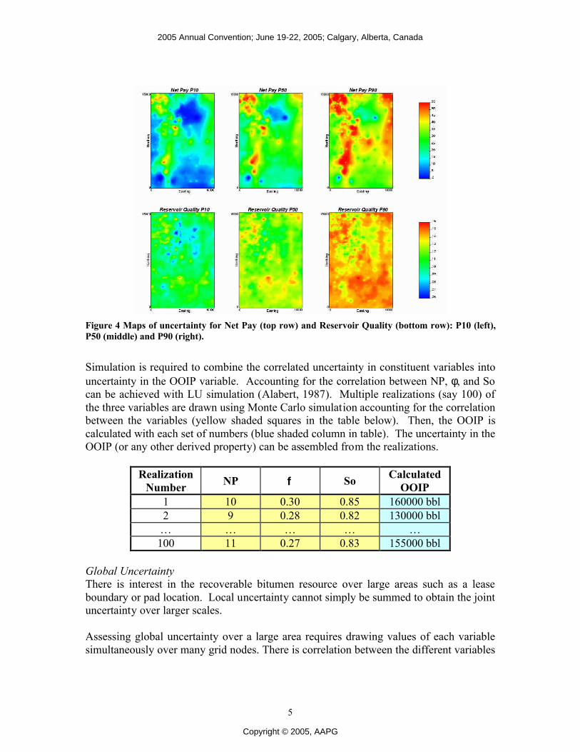
Simulation is required to combine the correlated uncertainty in constituent variables into uncertainty in the OOIP variable. Accounting for the correlation between NP, φ, and So can be achieved with LU simulation (Alabert, 1987). Multiple realizations (say 100) of the three variables are drawn using Monte Carlo simulation accounting for the correlation between the variables (yellow shaded squares in the table below). Then, the OOIP is calculated with each set of numbers (blue shaded column in table). The uncertainty in the OOIP (or any other derived property) can be assembled from the realizations.

Realization Number NP φ So Calculated

OOIP 1 10 0.30 0.85 160000 bbl 2 9 0.28 0.82 130000 bbl

… … … … … 100 11 0.27 0.83 155000 bbl

Global Uncertainty There is interest in the recoverable bitumen resource over large areas such as a lease boundary or pad location. Local uncertainty cannot simply be summed to obtain the joint uncertainty over larger scales. Assessing global uncertainty over a large area requires drawing values of each variable simultaneously over many grid nodes. There is correlation between the different variables



6

(as described above) and spatial correlation between the locations of interest. The LU simulation method could also be used to model this joint multivariate and spatial correlation; however, the number of variables and locations quickly becomes large and computationally expensive. For this reason, a P-field simulation (Srivastava, 1992) technique is combined with LU simulation to perform the spatial/multivariate simulation. The key idea is to simulate a set of spatially correlated probability values (a “p-field”) and then simultaneously drawing the variable of interest at multiple locations. The LU decomposition is used to account for the multivariate correlations. The resulting sets of multiple variables can be used to assess uncertainty over arbitrarily large volumes. Conclusion A 2-D geostatistical modeling process within a Bayesian updating workflow is developed and used to characterize reservoir potential of a McMurray formation lease area. Different maps were created to reveal different aspects of the reservoir properties and their uncertainty. Trend maps and prior maps can be used to understand the variability of the reservoir parameter independent of any secondary information. The likelihood maps can be used to show the information from the secondary data. The updated maps contain the information from the well data as well as from the secondary data. The local uncertainty is accessed by the 2-D models, and P10, P50, and P90 maps provide heterogeneity and uncertainty information on the reservoir properties. The joint uncertainty can be assessed by a combination of the LU and p-field simulation methods. Acknowledgements The authors thank NSERC and the industry sponsors of the Centre for Computational Geostatistics for supporting this research. References F.G. Alabert, The practice of fast conditional simulations through the LU decomposition of the covariance matrix, Mathematical Geology, 19(5), p. 369-386, 1987 C.V. Deutsch and A.G. Journel, GSLIB: Geostatistical Software Library and User’s Guide, Oxford University Press, New York, 1998 J. McLennan and C.V. Deutsch, Guide to SAGD Reservoir Characterization Using Geostatistics, Center for Computational Geostatistics, University of Alberta, Edmonton, Alberta, April 2003 C.V. Deutsch and S. Zanon, Direct Predication of Reservoir Performance with Bayesian Updating Under a Multivariate Gaussian Model. Paper presented at the Petroleum Society’s 5th Canadian International Petroleum Conference (55th Annual Technical Meeting), Calgary, Alberta, Canada, June 8 – 10, 2004. Srivastava, R. M., Reservoir characterization with probability field simulation: SPE Formation Evaluation, 7(4), p. 927–937, 1992.



Documents

Reservoir Characterization of McMurry Formation by 2-D