Embed Size (px)
Citation preview
HAL Id: tel-01284476https://tel.archives-ouvertes.fr/tel-01284476
Submitted on 7 Mar 2016
HAL is a multi-disciplinary open accessarchive for the deposit and dissemination of sci-entific research documents, whether they are pub-lished or not. The documents may come fromteaching and research institutions in France orabroad, or from public or private research centers.
L’archive ouverte pluridisciplinaire HAL, estdestinée au dépôt et à la diffusion de documentsscientifiques de niveau recherche, publiés ou non,émanant des établissements d’enseignement et derecherche français ou étrangers, des laboratoirespublics ou privés.
Modeling and experimental validation of hightemperature steam and carbon dioxide co-electrolysis
Jerôme Aicart
To cite this version:Jerôme Aicart. Modeling and experimental validation of high temperature steam and carbon dioxideco-electrolysis. Other. Université de Grenoble, 2014. English. NNT : 2014GRENI095. tel-01284476

THÈSE
Pour obtenir le grade de
DOCTEUR DE L’UNIVERSITÉ DE GRENOBLE
Spécialité : Ingénierie – Matériaux Mécanique Énergétique Environnement Procédés Production
Arrêté ministériel : 7 août 2006
Présentée par
Jérôme AICART Thèse dirigée par Laurent DESSEMOND et codirigée par Jérôme LAURENCIN et Marie PETITJEAN préparée au sein du CEA LITEN et du LEPMI dans l'École Doctorale IMEP2
Modélisation et Validation Expérimentale de la Co-Électrolyse de la Vapeur d’Eau et du Dioxyde de Carbone à Haute Température
Thèse soutenue publiquement le 03 Juin 2014, devant le jury composé de :
M. Gilles CABOCHE Professeur, Université de Bourgogne, Président du Jury
M. Olivier LOTTIN Professeur, Université de Lorraine LEMTA, Rapporteur
Mme. Armelle RINGUEDE Docteur, Chimie ParisTech, Rapporteur
M. Jan VAN HERLE Docteur, EPFL Lausanne, Examinateur
M. Yann BULTEL Professeur, Grenoble-INP LEPMI, Examinateur
Mme. Sandra CAPELA Docteur, GDF SUEZ, Membre invité
M. Laurent DESSEMOND Professeur Grenoble-INP LEPMI, Directeur de thèse M. Jérôme LAURENCIN Docteur, CEA LITEN, Co-encadrant de thèse
Mme. Marie PETITJEAN Docteur, CEA LITEN, Co-encadrant de thèse

i
ii
Abstract
This work investigates the high temperature co-electrolysis of H2O and CO2 in Solid Oxide
Cells. A detailed model was developed, encompassing electrochemical, chemical, thermal and
mass transfer phenomena, and introducing a macroscopic representation of the co-electrolysis
mechanism. This model allows predicting the performances and outlet compositions in single
cell and stack environments. An experimental validation protocol was implemented on two
types of commercial Cathode Supported Cells, ranging from polarization curves, obtained in
single and co-electrolysis modes, to micro gas analyses. These tests aimed both at determining
the different exchange current densities, representative of the kinetics of electrochemical
reactions, and validating the simulated cell global behavior and mechanism proposed.
Comprehensive analysis of the simulations led to the identification of limiting processes and
paths for optimization, as well as to the establishment of co-electrolysis operating maps.
Résumé
Cette étude porte sur la co-électrolyse de H2O et CO2 à 800°C dans une cellule à oxydes
solides. Un modèle détaillé a été développé afin de rendre compte des phénomènes
électrochimiques, chimiques, thermiques et de transferts de matière, et introduisant une
représentation macroscopique du mécanisme de co-électrolyse. Il permet d’estimer les
performances et les compositions en sortie de cellule. Un protocole expérimental, visant à
valider les principales hypothèses de ce modèle, a été appliqué à deux types de cellule
commerciale à cathode support. À partir de courbes de polarisations, obtenues en électrolyse
et en co-électrolyse, ainsi que d’analyses gaz, les densités de courant d’échange, illustrant les
cinétiques électrochimiques, ont pu être estimées, et le mécanisme proposé a pu être validé.
L’analyse des simulations a permis l’identification des processus limitant la co-électrolyse, la
proposition de voies d’optimisation et l’établissement des cartographies de fonctionnement.
iii
« Le monde est composé de flèches et de molécules, et d'électricité,
comme le Big-Bang tu vois, et tout ça ensemble, ça forme l'Univers. »
Jean-Claude Van Damme
« Trèfle à Quatre Feuilles »
Grille de nickel assurant le contact électrique avec la cellule électrochimique.
Marque laissée par la combustion de l’hydrogène dans l’air passant par une fissure en forme d’étoile.
« Four-Leaf Clover »
Nickel grid providing electrical contact with the electrochemical cell.
Mark left by the combustion of hydrogen in air flowing through a star shaped crack.
The journey is the reward.
Chinese Proverb

iv
Acknowledgements
-
Remerciements

v
Ces travaux s’étant déroulés principalement au CEA de Grenoble, je tiens au préalable à
remercier Mme Julie MOUGIN, pour son accueil au sein du laboratoire LTH.
Mes plus vifs remerciements vont également à Mme Armelle RINGUEDE et
M. Olivier LOTTIN pour avoir accepté de rapporter ce travail, à M. Jan VAN HERLE,
M. Yann BULTEL et Mme Sandra CAPELA pour leur participation au jury de soutenance,
ainsi qu’à M. Gilles CABOCHE pour l’avoir présidé.
Je voudrais remercier « du fond du cœur » Marie PETITJEAN, Jérôme LAURENCIN,
ainsi que mon directeur de thèse Laurent DESSEMOND, pour l’encadrement exceptionnel
dont j’ai bénéficié durant ces trois années. Vous avez su me faire confiance en me laissant la
liberté et l’autonomie que je cherchais, tout en restant présents, actifs et réactifs.
Votre bonne humeur, entente et investissement sous-tendent ce travail, votre plus grande
qualité ayant sans doute été de m’avoir supporté tout au long de ce périple. Dans les moments
de joie comme dans ceux de doutes et de galères, bien nombreux, vous avez été d’un soutien
inébranlable. Et bien que vos travaux individuels s’inscrivent dans des contextes différents,
vous êtes parvenus à être continuellement d’accord, ce qui n’était parfois pas une mince
affaire.
Ces travaux n’auraient jamais pu être ce qu’ils sont sans le dévouement infaillible d’une bien
belle équipe de techniciens. Je cite Benoit SOMMACAL pour son aide précieuse dans la
mise en place du banc, Michel PLANQUE pour ses talents de dessinateur,
André CHATROUX pour son habileté à murmurer à l’oreille des automates, ou encore
Lionel TALLOBRE pour sa contribution soutenue qui nous a permis d’obtenir des mesures
chromatographiques de grande qualité. Et bien sûr Pascal GIROUD ! Un simple signe de
ponctuation ne suffit pas, bien sûr, à exprimer toute ma gratitude. Tes petits doigts de fée
m’ont sorti de nombreuses situations délicates, dont la liste justifierait un second manuscrit.
Après tout, « il n’y a pas de problème, il n’y a que des solutions ».
Je n’oublie pas Bertrand MOREL, pour ses conseils éclairés lors de nos nombreuses
discussions autour des bancs. J’ai beaucoup appris de toi et de ton souci constant d’une
expérience bien maîtrisée. Ma sympathie va également à Stéphane DI IORIO et à
Karine COUTURIER, pour leurs remarques pertinentes et avisées, leur jovialité et leur
expertise, tant sur les oxydes solides que sur la trompette ou le violon.
Ma plus grande gratitude va également à Magali REYTIER, pour son implication, son
investissement, et sa fantastique force de proposition. A chaque obstacle, tu avais plus de
solutions que je ne pouvais explorer. Je te souhaite plein de belles réussites et beaucoup de
courage pour avoir pris la tête de la joyeuse bande du LPH.
vi
Ma chaleureuse reconnaissance va également à Sarah LORAUX, pour sa rigueur et son
soutien, qui débordent largement ses missions de secrétariat. Nous avons parfois bravé les
intempéries, et ces moments partagés étaient pour moi une vraie bouffée d’oxygène.
Je ne peux citer individuellement tous ceux qui, lors de discussions de couloirs, de
collaborations ponctuelles ou informelles, ou simplement grâce à la cohésion qui existe dans
ce laboratoire, m’ont apporté réflexions et bénéfices constructifs. Je vous remercie donc tous
infiniment, membres du LTH, du D2 et d’ailleurs ! Je garderai en mémoire, preuve de
l’ambiance générale, les « tourments » de trouver une table de 20 le midi.
Comment continuer ces remerciements sans parler du bureau des thésards. En partageant le
fameux bureau D2-214 avec toi, Myriam DE SAINT JEAN, et toi, François USSEGLIO-
VERETTA, la pièce semblait bien plus grande. Je vous souhaite réussite et succès pour votre
soutenance prochaine.
Ensuite, je souhaiterais exprimer ma reconnaissance à Élisabeth DJURADO ainsi qu’à
l’ensemble du personnel de l’équipe IES du LEPMI. En m’accueillant parmi vous durant
quelques mois, j’ai beaucoup appris à vos côtés, notamment la facette académique de la
recherche, inconnue pour moi jusqu’alors.
Je voudrais également faire part de ma gratitude à Romain SOULAS. Tu as transformé une
conversation autour d’un verre en clichés MEB et analyses chimiques de mes cellules, tout en
m’expliquant ce que tu faisais. Que ne l’ai-je su avant !
Et parce que le CEA finissait par fermer le soir, merci à Bob, Clairette, Coco, Elise, Ju,
Junior, Mathilde, Rem, Seb, Serguei et tous les autres, pour votre soutien et votre amitié. Sans
vous, j’aurais probablement été plus reposé certains matins…
Enfin, j’adresse toute mon affection à ma famille, Lucile, Pauline, Patrick et Christine, pour
leur confiance, leur tendresse et leur soutien sans faille durant ces 3 années, ainsi que les 25
qui les ont précédées. Pour ne citer que quelques détails parmi l’immensité du tout, Lucile,
ton expertise a métamorphosé la présentation, la faisant passer de « oh mais quelle horreur ! »
à ce qu’elle est devenue, et Maman, ce pot était magnifique.
Enfin, à tous ceux que j’ai pu oublier, et à vous tous déjà évoqués, un grand merci pour votre
contribution, quelle qu’elle ait pu être, dans ce qui s’est avéré être une grande et très belle
aventure.

vii

viii
Table of Contents
ix
Chapter 1 - Introduction…………………………...p.1
1.1. From Fossil Carbonated Energies to Environmental Pressures ............................................... 3
1.2. Integration of Carbon-Free Energies ....................................................................................... 8
1.3. Electrolysis Technologies ...................................................................................................... 11
1.3.1. High Temperature Steam Electrolysis ........................................................................... 14
1.3.2. High Temperature Carbone Dioxide Electrolysis ......................................................... 17
1.3.3. High Temperature H2O and CO2 Co-Electrolysis ......................................................... 18
1.4. Overview of a Solid Oxide Electrolysis Cell ........................................................................ 21
1.4.1. Steady State ................................................................................................................... 21
1.4.2. Overpotentials and Polarization Curves Decomposition ............................................... 22
1.4.3. Electrochemical Reactions ............................................................................................ 24
1.4.4. Mass Transport .............................................................................................................. 25
1.5. Objectives of the Study ......................................................................................................... 27
1.6. Methodology ......................................................................................................................... 28
1.7. References ............................................................................................................................. 29
Chapter 2 - State of the Art………………………p.33
2.1. SOC Materials ....................................................................................................................... 36
2.1.1. Electrolyte ..................................................................................................................... 37
2.1.2. Fuel Electrode ................................................................................................................ 38
2.1.3. Oxygen Electrode .......................................................................................................... 39
2.2. Recent Experimental Developments ..................................................................................... 40
2.2.1. Performances ................................................................................................................. 40
2.2.2. Durability and Degradation ........................................................................................... 43
2.2.2.1. Experimental Reports ............................................................................................ 43
2.2.2.2. Carbon Deposition ................................................................................................. 44
2.3. Modeling Studies ................................................................................................................... 45
2.4. References ............................................................................................................................. 47

x
Chapter 3 - Tools………………………………….p.52
3.1. Experimental Setup for Cell Testing ..................................................................................... 55
3.1.1. Test Bench ..................................................................................................................... 55
3.1.2. Gas Lines, Steam Generation and Gases Purity ............................................................ 56
3.1.3. Safety Concerns Related to Gases ................................................................................. 57
3.1.4. Measuring Equipment ................................................................................................... 58
3.1.4.1. Polarization Curves ............................................................................................... 59
3.1.4.2. Gas Analyses ......................................................................................................... 59
3.1.4.3. Electrochemical Impedance Spectroscopy (EIS)................................................... 60
3.1.5. Cell Startup Procedures ................................................................................................. 60
3.1.5.1. Test Bench Tightness Evaluation .......................................................................... 60
3.1.5.2. Temperature Changes and Glass Ceramic Sealing Procedure ............................... 61
3.1.5.3. Cermet Reduction .................................................................................................. 61
3.1.5.4. Mechanical Load Optimization ............................................................................. 62
3.2. Modeling Approach ............................................................................................................... 63
3.2.1. Geometry and Materials ................................................................................................ 63
3.2.2. Mass Transfer Description ............................................................................................ 65
3.2.3. Electrochemical Description ......................................................................................... 68
3.2.4. Thermal Description ...................................................................................................... 72
3.2.5. Numerical Architecture ................................................................................................. 76
3.2.6. Numerical Reliability .................................................................................................... 77
3.2.6.1. Loops on Each Current Density............................................................................. 77
3.2.6.2. Loop on Global Current Density Stability ............................................................. 78
3.2.6.3. Loop on Counter Flow ........................................................................................... 78
3.3. Conclusion ............................................................................................................................. 78
xi
Chapter 4 - Model Validation…………………….p.82
4.1. Model Version ....................................................................................................................... 86
4.2. Investigations of a CSC with a Known Microstructure (FZJ) ............................................... 86
4.2.1. Cell ................................................................................................................................ 87
4.2.2. Experiments ................................................................................................................... 88
4.2.3. Cell Stability .................................................................................................................. 89
4.2.4. Polarization curves for H2O and CO2 single electrolyses .............................................. 90
4.2.5. Determination of Cathodic ‘Apparent’ Exchange Current Densities ............................ 91
4.2.5.1. Steam Electrolysis ................................................................................................. 92
4.2.5.2. Carbon Dioxide Electrolysis .................................................................................. 94
4.2.6. Prediction of Cell Behavior in Co-Electrolysis Mode ................................................... 95
4.2.7. Steam Outlet Mass Balance in Co-Electrolysis Operation ............................................ 96
4.2.8. Intermediate Conclusions .............................................................................................. 97
4.3. Investigations of a CSC with Unknown Microstructure (Optimized Cell) ........................... 98
4.3.1. Methodology ................................................................................................................. 98
4.3.2. Cell ................................................................................................................................ 98
4.3.3. Experiments ................................................................................................................... 99
4.3.4. Cell Stability ................................................................................................................ 100
4.3.5. Experimental and Simulated single electrolyses polarization curves .......................... 101
4.3.5.1. Determination of Cathode Tortuosity Factor and .................................. 102
4.3.5.2. Determination of .................................................................................... 104
4.3.6. Comparison of experimental and simulated co-electrolysis i-V curves ....................... 105
4.3.7. Gas analysis – WGSR kinetics validation ................................................................... 106
4.3.8. Gas analysis – Galvanostatic Operation ...................................................................... 109
4.3.9. Gas analysis – Effect of the Current Density .............................................................. 111
4.3.10. Sensitivity Analysis ..................................................................................................... 114
4.4. Conclusion ........................................................................................................................... 117
4.5. References ........................................................................................................................... 118
2
0,
CO CO
cathodei
2 2
0,
H H O
cathodei

xii
Chapter 5 - Simulation Results & Discussion….p.120
5.1. Investigation of Co-Electrolysis Mechanism ...................................................................... 123
5.1.1. High Faradic Conversion ............................................................................................. 123
5.1.1.1. Evolutions Along the Cell Radius ....................................................................... 124
5.1.1.2. Evolutions Along the Cathode Thickness ........................................................... 127
5.1.2. Effect of Polarization ................................................................................................... 128
5.1.3. Co-electrolysis Simulated Performances at 800°C ...................................................... 131
5.2. Intermediate Conclusion ...................................................................................................... 133
5.3. SRU Operation .................................................................................................................... 134
5.3.1. Simulation Parameters ................................................................................................. 135
5.3.2. Polarization Curve at 20 NmL.min-1
.cm-2
.................................................................... 137
5.3.3. Overpotentials Decomposition .................................................................................... 139
5.3.4. Longitudinal Evolutions of Cell Temperature ............................................................. 140
5.3.5. Longitudinal Evolutions of Molar Fractions and β ..................................................... 141
5.3.6. Co-electrolysis Operating Maps .................................................................................. 143
5.3.7. Influence of Inlet Ratio CO2/H2O ................................................................................ 147
5.4. Conclusion ........................................................................................................................... 148
5.5. References ........................................................................................................................... 150
xiii
Chapter 6 - Conclusion………………………….p.152
Chapter 7 - Appendix……………………………p.158
7.1. Hysteresis on Optimized Cell .............................................................................................. 161
7.1.1. Influence of Composition and Time ............................................................................ 161
7.1.2. Influence of Limiting Current ..................................................................................... 163
7.1.3. Conclusion ................................................................................................................... 164
7.2. Cell Degradation in Co-Electrolysis .................................................................................... 165
7.2.1. Durability Experiment : 900 h at -1 A.cm-2
.................................................................. 165
7.2.2. SEM Analysis .............................................................................................................. 167
7.3. Steam Electrolysis Operating Maps .................................................................................... 171
7.4. References ........................................................................................................................... 174

xiv
Table of Figures
xv
Chapter 1 - Introduction
Figure 1-1: Correlation between atmospheric CO2 concentration and global temperature changes ....... 4
Figure 1-2: Atmospheric concentrations of CO2, CH4 and N2O.............................................................. 5
Figure 1-3: Distribution of the world energy consumption ..................................................................... 6
Figure 1-4: Oil prices fluctuations over the past 150 years and reserve to production ratios ................. 7
Figure 1-5: Current technologies for electricity storage .......................................................................... 9
Figure 1-6: “Power to gas” ecosystem (European project Sophia) ......................................................... 9
Figure 1-7: Components of a typical SOEC .......................................................................................... 12
Figure 1-8: Evolution of the total energy demand, electrical energy demand and heat demand with
temperature for steam electrolysis ......................................................................................................... 15
Figure 1-9: Temperature of an operating SRU - thermal operating modes for steam electrolysis ........ 16
Figure 1-10: Principles of H2O electrolysis, CO2 electrolysis and co-electrolysis. ............................... 19
Figure 1-11: Typical decomposition of polarization curves in both SOFC and SOEC ......................... 23
Figure 1-12: Triple Phase Boudary lengths (TPBl). .............................................................................. 24
Figure 1-13: Illustration of the geometrical tortuosity factor. ............................................................... 26
Figure 1-14: H2O and H2 paths along the cell and trough the cathode in steam electrolysis ................ 26
Figure 1-15: Summary of the methodology implemented. .................................................................... 28

xvi
Chapter 2 - State of the Art
Figure 2-1: Ternary C-O-H diagram at 1 atm with typical co-electrolysis inlet compositions ............. 44
Chapter 3 - Tools
Figure 3-1: Description of the experimental setup in the vicinity of the cell. ....................................... 56
Figure 3-2: Schematic of the complete test bench. ................................................................................ 56
Figure 3-3: Health risks of carbon monoxide ........................................................................................ 58
Figure 3-4: OCV evolution during cermet reduction at 800°C ............................................................. 62
Figure 3-5: Schematic representation of the simulated SRU considering a planar electrolyte-supported
cell in a counter-flow configuration ...................................................................................................... 64
Figure 3-6: Schematic representation of the simulated SRU considering a radial cathode-supported cell
in a co-flow configuration ..................................................................................................................... 64
Figure 3-7: Equivalent electrical circuit for cell operation in co-electrolysis mode. ............................ 68
Figure 3-8: Boundary conditions assumed for the thermal simulations ................................................ 73
Figure 3-9: Isothermal model summary and architecture ...................................................................... 77
Figure 3-10: Complete model summary and architecture ..................................................................... 77
xvii
Chapter 4 - Model Validation
Figure 4-1: Representation of the three-dimensional reconstructed microstructure of the studied Ni-
8YSZ support ........................................................................................................................................ 87
Figure 4-2: Evolution of the polarization curve A1 throughout the electrochemical protocol.............. 89
Figure 4-3: Experimental polarization curves for H2O electrolysis A1-A4. ......................................... 91
Figure 4-4: Experimental polarization curves for CO2 electrolysis A5-A8........................................... 91
Figure 4-5: Simulations A1 to A4 with all model inputs set ( 2 2
0,
H H O
cathodei
= 530 mA.cm-²). ........................ 93
Figure 4-6: Experimental and simulated polarization curves for experiment A4. ................................ 93
Figure 4-7: Simulations A5 to A8 with computed
2
0,
CO CO
cathodei . .................................................................. 94
Figure 4-8: Experimental and simulated polarization curves for experiment A8. ................................ 94
Figure 4-9: Experimental and simulated polarization curves for experiment A9. ................................ 96
Figure 4-10: Experimental and simulated polarization curves for experiment A10.............................. 96
Figure 4-11: SEM examination of the optimized cell cermet ............................................................... 99
Figure 4-12: Evolution of the polarization curve B1 throughout the electrochemical protocol .......... 101
Figure 4-13: Experimental and simulated polarization curves B5, B6 and B6* for CO2 electrolysis . 103
Figure 4-14: Experimental and simulated polarization curves B1, B2 and B2* for H2O electrolysis . 105
Figure 4-15: Experimental and simulated polarization curves B3*. .................................................. 106
Figure 4-16: Experimental and simulated polarization curves B4*. .................................................. 106
Figure 4-17: Diagram of the test bench in the cell vicinity ................................................................. 107
Figure 4-18: Experimental and simulated µGC composition corresponding to experiment SExp.4 .. 108
Figure 4-19: Experimental and simulated µGC compositions for experiments SExp.1-3. ................. 109
Figure 4-20: Gas chromatography results in stationary conditions over 288 h with B3* composition
and flow (48/16/16/20 vol.% H2O/CO2/H2/N2, -0.67 A.cm-2
– 24.3% faradic conversion) ................. 110
Figure 4-21: Evolution of the cell voltage during the 288 h steady state experiment at -0.67 A.cm-2
. 111
Figure 4-22: Gas chromatography analyses and simulated outlet compositions ................................. 112
Figure 4-23: Evolution of steam molar fraction at the cell outlet with polarization. .......................... 113
Figure 4-24: Simulated polarization curves at 800°C for all study cases A, C, D and E .................... 115
Figure 4-25: Sensitivity analysis results at -1 A.cm-2
. ......................................................................... 115
Figure 4-26: Sensitivity analysis results at -1.5 A.cm-2
. ...................................................................... 115
xviii
Chapter 5 - Simulation Results & Discussion
Figure 5-1: Molar fractions along the cathode/electrolyte interface for simulated experiment A10 (co-
electrolysis) at 1300 mV. ..................................................................................................................... 124
Figure 5-2: Current densities along the cell radius for simulated experiment A10 (co-electrolysis) at
1300 mV. .............................................................................................................................................. 124
Figure 5-3: Overpotentials related to H2O electrolysis along the cell radius for simulated experiment
A10 (co-electrolysis) at 1300 mV. ....................................................................................................... 126
Figure 5-4: Resulting local rate of the WGS reaction along the cell radius for simulated Experiment
A10 (co-electrolysis) at 1300 mV. ....................................................................................................... 127
Figure 5-5: Molar fractions in the cathode thickness, at 8.5 mm (middle) of cell radius, for simulated
Experiment A10 (co-electrolysis) at 1300 mV. ................................................................................... 128
Figure 5-6: WGS reaction production rate in the cathode thickness, at 8.5 mm (middle) of cell radius,
for simulated Experiment A10 (co-electrolysis) at 1300 mV .............................................................. 128
Figure 5-7: CO relative production by R-WGS reaction for simulated experiment A10 as a function of
polarization .......................................................................................................................................... 129
Figure 5-8: Overpotentials related to H2O electrolysis for simulated Experiment A10. .................... 130
Figure 5-9: Simulated performances for all electrolysis modes at 800°C (6 NmL.min-1
.cm-2
). .......... 131
Figure 5-10: Simulated performances for all electrolysis modes at 800°C (12 NmL.min-1
.cm-2
). ...... 131
Figure 5-11: CO relative production by R-WGS for simulated composition 65/25/10 vol.% of
H2O/CO2/H2 ......................................................................................................................................... 132
Figure 5-12: Geometry of the simulated SRU – CSC in counter-flow configuration. ........................ 134
Figure 5-13: Influence of the operating temperature on the SRU performances ................................ 138
Figure 5-14: Decomposition of C2 polarization curve ........................................................................ 139
Figure 5-15: Longitudinal evolutions of cell temperature as a function of the cell voltage ................ 140
Figure 5-16: Molar fractions along the cathode/electrolyte interface and β longitudinal evolutions at
1.4 V when the cell is fed with 20 NmL.min-1
.cm-2
of 65/25/10 vol.% H2O/CO2/H2 .......................... 142
Figure 5-17: Co-electrolysis operating maps (1/4): Current densities and corresponding Faradic
conversion rates ................................................................................................................................... 145
Figure 5-18: Co-electrolysis operating maps (2/4): Production of H2 and CO and Efficiency ........... 145
Figure 5-19: Co-electrolysis maps (3/4): Heat source terms and Middle cell Temperature ................ 146
Figure 5-20: Co-electrolysis operating maps (4/4): CO produced by the reverse WGS reaction
compared to CO2 electrolysis and H2/CO ratio at the cell outlet ......................................................... 146
Figure 5-21: Outlet compositions simulated at 1.3 V with the isothermal model, as a function of the
inlet ratio CO2/H2O. ............................................................................................................................. 147
xix
Chapter 7 - Appendix
Figure 7-1: Effect of inlet composition of hysteresis in all electrolysis modes at 800°C ................... 161
Figure 7-2: Hysteresis resulting from CO2 electrolysis obtained at 800°C on 2 cells. ........................ 162
Figure 7-3: Influence of reaching the limiting current density on i-V hysteresis. ............................... 163
Figure 7-4: Durability experiment in H2O and co-electrolysis modes over nearly 1000 h in
galvanostatic operation (-1 A.cm-2
, 24 NmL.min-1
.cm-2
, 90/10 vol.% H2O/H2 (+20% N2) and
65/25/10 vol.% H2O/CO2/H2) .............................................................................................................. 166
Figure 7-5: MEB examinations of the reference reduced cermet. ....................................................... 168
Figure 7-6: MEB examinations of the cathode/electrolyte interface vicinity of a used cell ............... 169
Figure 7-7: MEB examination of the cell used in the durability experiment, ................................... 170
Figure 7-8: Steam electrolysis operating maps (1/3): Current density and H2 production ................. 171
Figure 7-9: Steam electrolysis operating maps (2/3): Conversion rate and Efficiency ...................... 172
Figure 7-10: Steam electrolysis operating maps (3/3): Longitudinal and Middle cell temperatures .. 173

xx
Table of Tables

xxi
Chapter 1 - Introduction
Table 1-1: Electricity production in Europe and evolution of Renewable Energy Sources .................... 8
Table 1-2: Energy content of different vectors ...................................................................................... 11
Table 1-3: Overview of some hydrogen production technologies......................................................... 13
Table 1-4: Overview of some CO production technologies from CO2. ................................................ 18
Table 1-5: Synthetic fuels produced via co-electrolysis of H2O+CO2 or steam electrolysis................. 19
Chapter 2 - State of the Art
Table 2-1: Overview of some performances and degradations reports in recent literature ................... 42
Chapter 3 - Tools
Table 3-1: Available characteristics of gases used in electrolysis investigations. ................................ 57
Table 3-2: Characteristics of carrier gas used in micro gas chromatography analyses ......................... 60
Table 3-3: Classical conditions for EIS scan recording ........................................................................ 60
Table 3-4 : Kinetic values for WGS reaction kinetics ........................................................................... 67
Chapter 4 - Model Validation
Table 4-1: Actual cermet microstructure obtained by X-ray nanotomography. .................................... 87
Table 4-2: Gas feeding conditions tested on the commercial FZJ CSC at T = 800°C. ......................... 88
Table 4-3: Values for adjusted on experimental data. ............................................................. 93
Table 4-4: Values of apparent exchange current density fitted on CO2/CO experimental data. ........... 94
Table 4-5: Summary of steam outlet mass balance experiment. ........................................................... 97
Table 4-6: Electrochemical experimental protocol.. ........................................................................... 100
Table 4-7: Microstructure parameters and ‘apparent’ exchange current densities .............................. 103
Table 4-8: Micro gas chromatography experimental protocol, results and simulations.. .................... 108
Table 4-9: Study cases for the sensitivity analysis. ............................................................................. 114
2 2
0,
H H O
cathodei

xxii
Chapter 5 - Simulation Results & Discussion
Table 5-1: Maximum simulated influence of the WGS reaction over CO or H2 production .............. 133
Table 5-2: Thermal simulations inputs ................................................................................................ 136
Table 5-3: Optimum inlet compositions for specific syngas production at 1300 mV. ........................ 148
Chapter 7 - Appendix
Table 7-1: Steam outlet mass balance experiment and µGC measurements in co-electrolysis operation
during the durability test. Comparison simulated and experimental data. .......................................... 166

xxiii

xxiv
Table of Symbols
xxv
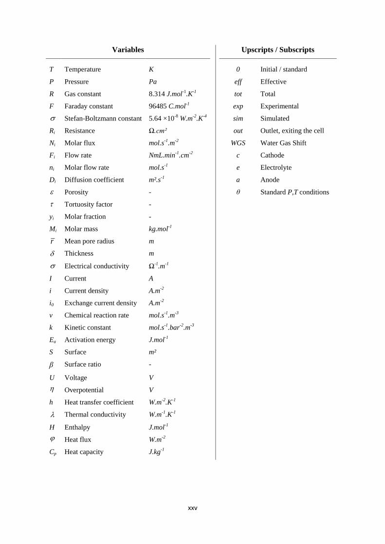
Variables
T Temperature K
P Pressure Pa
R Gas constant 8.314 J.mol-1
.K-1
F Faraday constant 96485 C.mol-1
Stefan-Boltzmann constant 5.64 ×10⁻⁸
W.m-2
.K-4
Ri Resistance Ω.cm²
Ni Molar flux mol.s-1
.m-2
Fi Flow rate NmL.min-1
.cm-2
ni Molar flow rate mol.s-1
Di Diffusion coefficient m².s-1
Porosity -
Tortuosity factor -
yi Molar fraction -
Mi Molar mass kg.mol-1
r Mean pore radius m
Thickness m
Electrical conductivity Ω-1
.m-1
I Current A
i Current density A.m-2
i0 Exchange current density A.m-2
v Chemical reaction rate mol.s-1
.m-3
k Kinetic constant mol.s-1
.bar-2
.m-3
Ea Activation energy J.mol-1
S Surface m²
β Surface ratio -
U Voltage V
Overpotential V
h Heat transfer coefficient W.m-2
.K-1
Thermal conductivity W.m-1
.K-1
H Enthalpy J.mol-1
Heat flux W.m-2
Cp Heat capacity J.kg-1
Upscripts / Subscripts
0 Initial / standard
eff Effective
tot Total
exp Experimental
sim Simulated
out Outlet, exiting the cell
WGS Water Gas Shift
c Cathode
e Electrolyte
a Anode
θ Standard P,T conditions

Chapter 1 – Introduction
1
Chapter 1
Introduction

Chapter 1 – Introduction
2
Chapter 1 – Introduction
3
Chapter 1
Introduction
1.1. From Fossil Carbonated Energies to Environmental Pressures .................................... 3
1.2. Integration of Carbon-Free Energies ............................................................................ 8
1.3. Electrolysis Technologies ............................................................................................ 11
1.3.1. High Temperature Steam Electrolysis ................................................................. 14
1.3.2. High Temperature Carbone Dioxide Electrolysis ................................................ 17
1.3.3. High Temperature H2O and CO2 Co-Electrolysis................................................ 18
1.4. Overview of a Solid Oxide Electrolysis Cell ................................................................ 21
1.4.1. Steady State ........................................................................................................ 21
1.4.2. Overpotentials and Polarization Curves Decomposition...................................... 22
1.4.3. Electrochemical Reactions .................................................................................. 24
1.4.4. Mass Transport ................................................................................................... 25
1.5. Objectives of the Study ............................................................................................... 27
1.6. Methodology ............................................................................................................... 28
1.7. References .................................................................................................................. 29
Chapter 1 – Introduction
4
1.1. From Fossil Carbonated Energies to
Environmental Pressures
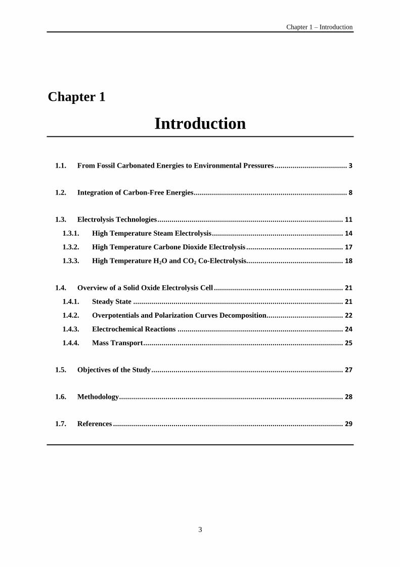
Icecap analyses over the past several hundreds of thousands of years have shown that there is
a strong correlation between the amount of CO2 in the atmosphere and average temperature
changes around the globe. As shown in Figure 1-1, the overall climate alternates from hot to
cold eras, and the temperature evolution follows remarkably the same pattern as the CO2 and
CH4 contents, which fluctuate from 180 to 300 ppmv and from 300 to 750 ppbv respectively
[1].
Figure 1-1: Correlation between atmospheric CO2 concentration and global temperature
changes [1].
Since the industrial revolution of the 19th
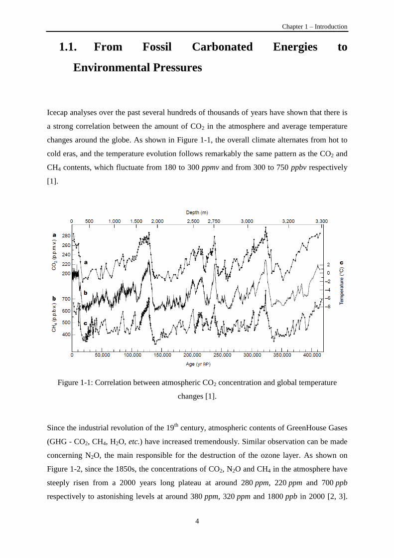
century, atmospheric contents of GreenHouse Gases
(GHG - CO2, CH4, H2O, etc.) have increased tremendously. Similar observation can be made
concerning N2O, the main responsible for the destruction of the ozone layer. As shown on
Figure 1-2, since the 1850s, the concentrations of CO2, N2O and CH4 in the atmosphere have
steeply risen from a 2000 years long plateau at around 280 ppm, 220 ppm and 700 ppb
respectively to astonishing levels at around 380 ppm, 320 ppm and 1800 ppb in 2000 [2, 3].
Chapter 1 – Introduction
5
The CO2 atmospheric content was 27% higher in 2000 than it has ever been over the past
400.000 years.
Figure 1-2:
Atmospheric concentrations of
CO2, CH4 and N2O [2, 3].
On the basis of this astounding increase of greenhouse gases concentration in the atmosphere,
climate models predict a global warming that could spread from 1.1°C to 6.4°C before the end
of the current century, depending on different scenario and CO2 emissions predictions [4].
Such an increase of the average global temperature could have unpredictable consequences:
mass extinction of species, rise of see level, mass migrations of populations, natural disaster
occurring more frequently, etc. Therefore, governments are trying to limit this temperature
increase, for instance by reducing GHG emissions. However, due to a lack of global
consensus and multi-country agreement, it seems that, within the 21st century, the world is
heading toward a 4°C temperature increase [5].
Most of mankind CO2 emissions are due to the massive use of fossil hydrocarbons to meet the
global energy bill. Indeed, as shown in Figure 1-3, more than 85% of the ever increasing
worldwide energy demand is provided by coal, oil and natural gas. Thus, these energy sources
remain vital for the economic development and social stability of most countries.

Chapter 1 – Introduction
6
Figure 1-3: Distribution of the world energy consumption [6].
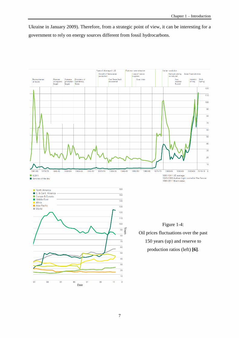
The price of oil (and therefore natural gas) has widely fluctuated throughout the past 150
years (Figure 1-4). It is currently sold for more than 100 $/barrel while the exchange rate was
as low as 10 current$/barrel in 1970. Any price peak can often be related to social or military
crises in the Middle East, such as the Iranian revolution in 1979, or more recently the invasion
of Afghanistan or the Arab Spring. The correlation between crises and oil prices stem from
the uneven worldwide distribution of the global oil reserves (Figure 1-4). Indeed, the Middle
East and South and Central America own the large majority of the world currently known oil
reserves, whereas Europe and Pacific Asia each have less than 30 years of estimated reserves.
Nowadays, the impact of uneven oil reserves distribution is reinforced by a global depletion
of resources, driven by a steadily increasing demand. Indeed, the known global oil stockpile is
estimated to last roughly 60 years (Figure 1-4). As oil is depleted, the exploitation of the
remaining wells will become more technical (deep under see level, underneath the polar ice
cap, etc.). Unless massive new reserves are discovered, the oil prices are likely to keep
increasing in the upcoming decades.
The oil cost and varying prices, along with the non-proportional distribution of the depleting
oil reserves can induce stress on the energy supply of most countries. In turn, this can lead to
diplomatic strains and eventually conflicts (e.g. Russia closing NG pipelines passing through
Chapter 1 – Introduction
7
Ukraine in January 2009). Therefore, from a strategic point of view, it can be interesting for a
government to rely on energy sources different from fossil hydrocarbons.
Figure 1-4:
Oil prices fluctuations over the past
150 years (up) and reserve to
production ratios (left) [6].
Years
Date
Chapter 1 – Introduction
8
1.2. Integration of Carbon-Free Energies
To decrease their carbonated fuel dependence, governments consider massive integration of
renewable energies in their global energy mix (Table 1-1).
Year 2010 2020 2030
Total (TWh) 3 335 3 540 3 706
RES (TWh) 715 1 217 1 689
RES/Total 21% 34% 46%
Table 1-1: Electricity production in Europe and evolution of Renewable Energy Sources
(RES)
(Source: IEA and Minerve Project).
Because most of renewable energy sources are constituted by small production units which
energy outputs fluctuate during the day/year, their integration on the global energy market
remains a major technological issue. Therefore, the portion of these small varying electricity
sources that cannot be directly injected in the global network (electrical grid) has to be stored
(using batteries or hydro pumps) to avoid wastage. Similar observations can be made
concerning nuclear energy. A nuclear reactor has a roughly constant energy output that cannot
be easily modulated to match the electricity network demand. Thus, the overproduction is
generally dumped or stored by pumping water. Without reliable and cost effective
technologies for energy storage, fluctuations of electricity demand on the grid can only be
managed using electrical sources generated from coal, natural gas or oil power plants, that
offer a larger flexibility compared to renewable or nuclear technologies.
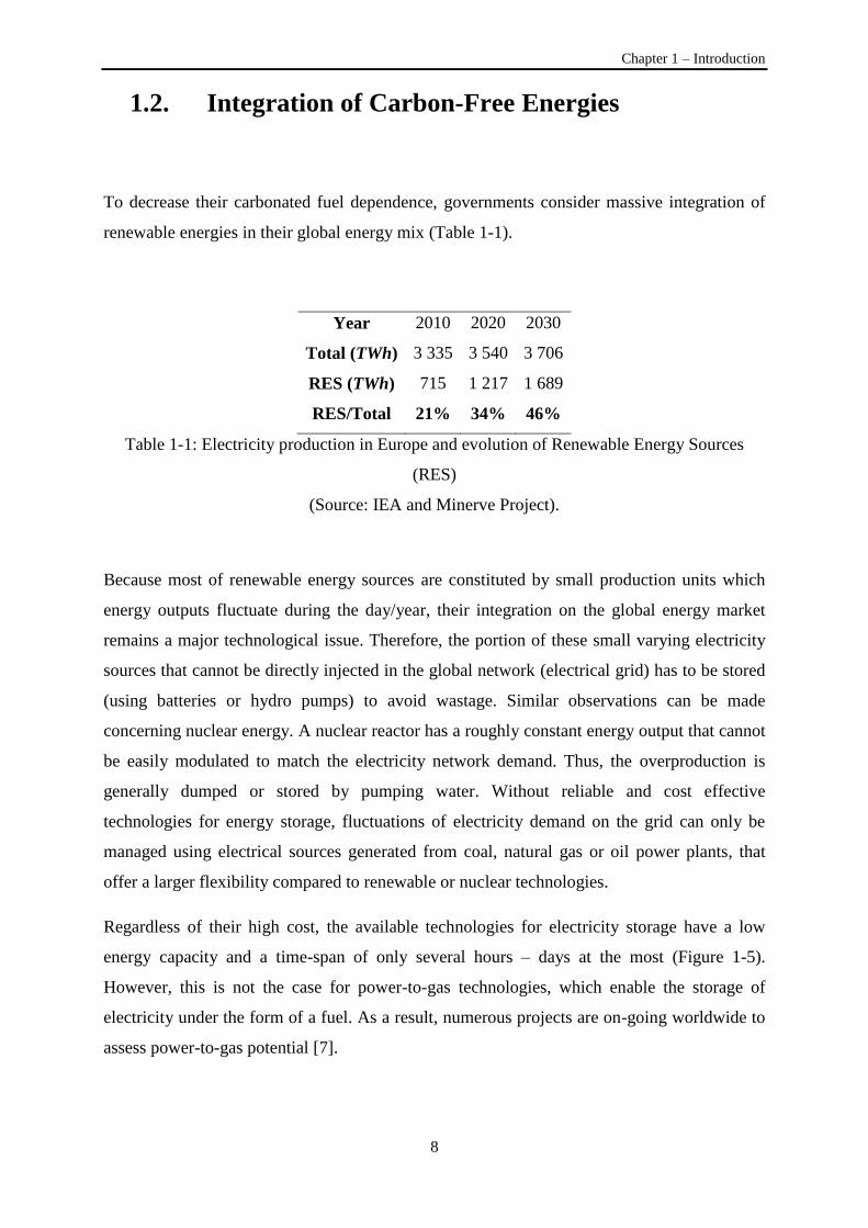
Regardless of their high cost, the available technologies for electricity storage have a low
energy capacity and a time-span of only several hours – days at the most (Figure 1-5).
However, this is not the case for power-to-gas technologies, which enable the storage of
electricity under the form of a fuel. As a result, numerous projects are on-going worldwide to
assess power-to-gas potential [7].
Chapter 1 – Introduction
9
Figure 1-5: Current technologies for electricity storage [8].
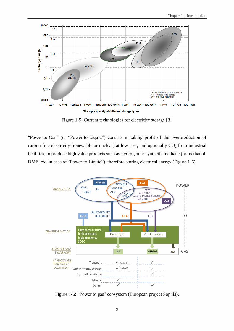
“Power-to-Gas” (or “Power-to-Liquid”) consists in taking profit of the overproduction of
carbon-free electricity (renewable or nuclear) at low cost, and optionally CO2 from industrial
facilities, to produce high value products such as hydrogen or synthetic methane (or methanol,
DME, etc. in case of “Power-to-Liquid”), therefore storing electrical energy (Figure 1-6).
Figure 1-6: “Power to gas” ecosystem (European project Sophia).
Chapter 1 – Introduction
10
There are a large number of applications and advantages in a “Power-to-Gas” vision, among
which are the following examples:
Hydrogen technologies and fuel cells are part of the European Strategic Energy
Technology Plan (Europe 2020 and Europe 2050). Hydrogen produced by electrolysis
and used for transport applications contributes to lowering GHG emissions and the
dependence of Europe on fossil mobility fuel. Several car manufacturers have
announced the commercialization of H2 vehicles embracing Europe’s vision.
Hythane makes storage and transport of hydrogen easy: in the near future, up to
20 vol.% hydrogen could be introduced in the existing natural gas network (making
Hythane) for domestic applications. This would thus participate to the lowering of
GHG emissions.
The development of energy storage technologies favors the deployment of renewable
energy by introducing flexibility to the electrical network, and helping offer to meet
demand. Storage also allows for high electrical network efficiency by ensuring that all
of the produced energy is consumed.
Synthetic gas, also called syngas (i.e. H2+CO), can be produced by electrolysis of H2O
and CO2 and further transformed into many end-products such as synthetic methane,
methanol or dimethyl ether (DME). These products can be used as fuels or by
industries (e.g. chemical industry). Co-electrolysis coupled with renewable or nuclear
power is not only a way to produce syngas; it can also valorize CO2 emitted by
industries such as steel, cement, and domestic waste incineration, which are numerous
and spread over Europe. Finally, oxygen by-product can further increase the added
value of the co-electrolysis process, if used for oxy-combustion purposes for example.
Hydrogen produced via water electrolysis opens up excellent perspectives for both storing
renewable/nuclear electricity and transport applications. Indeed, H2 has an extremely high
energy content per mass unit (although low energy content per volume unit), about three
times as high as gasoline (Table 1-2). Such energy feature makes it a serious option to be used
as a replacement fuel in “power to gas” scenarios.
Chapter 1 – Introduction
11
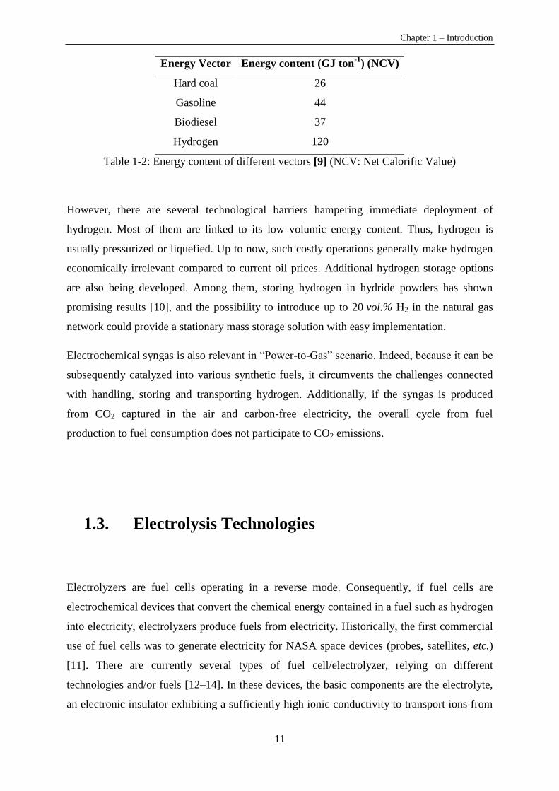
Energy Vector Energy content (GJ ton-1
) (NCV)
Hard coal 26
Gasoline 44
Biodiesel 37
Hydrogen 120
Table 1-2: Energy content of different vectors [9] (NCV: Net Calorific Value)
However, there are several technological barriers hampering immediate deployment of
hydrogen. Most of them are linked to its low volumic energy content. Thus, hydrogen is
usually pressurized or liquefied. Up to now, such costly operations generally make hydrogen
economically irrelevant compared to current oil prices. Additional hydrogen storage options
are also being developed. Among them, storing hydrogen in hydride powders has shown
promising results [10], and the possibility to introduce up to 20 vol.% H2 in the natural gas
network could provide a stationary mass storage solution with easy implementation.
Electrochemical syngas is also relevant in “Power-to-Gas” scenario. Indeed, because it can be
subsequently catalyzed into various synthetic fuels, it circumvents the challenges connected
with handling, storing and transporting hydrogen. Additionally, if the syngas is produced
from CO2 captured in the air and carbon-free electricity, the overall cycle from fuel
production to fuel consumption does not participate to CO2 emissions.
1.3. Electrolysis Technologies
Electrolyzers are fuel cells operating in a reverse mode. Consequently, if fuel cells are
electrochemical devices that convert the chemical energy contained in a fuel such as hydrogen
into electricity, electrolyzers produce fuels from electricity. Historically, the first commercial
use of fuel cells was to generate electricity for NASA space devices (probes, satellites, etc.)
[11]. There are currently several types of fuel cell/electrolyzer, relying on different
technologies and/or fuels [12–14]. In these devices, the basic components are the electrolyte,
an electronic insulator exhibiting a sufficiently high ionic conductivity to transport ions from
Chapter 1 – Introduction
12
one electrode to the other, and the electronic conductive electrodes, where electrochemical
reactions occur.
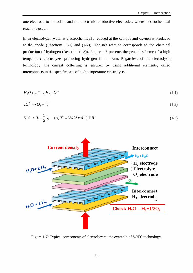
In an electrolyzer, water is electrochemically reduced at the cathode and oxygen is produced
at the anode (Reactions (1-1) and (1-2)). The net reaction corresponds to the chemical
production of hydrogen (Reaction (1-3)). Figure 1-7 presents the general scheme of a high
temperature electrolyzer producing hydrogen from steam. Regardless of the electrolysis
technology, the current collecting is ensured by using additional elements, called
interconnects in the specific case of high temperature electrolysis.
2
2 22H O e H O (1-1)
2
22 4O O e (1-2)
1
2 2 2
1 286 .
2rH O H O H kJ mol [15] (1-3)
Figure 1-7: Typical components of electrolyzers: the example of SOEC technology.
H2O+ H2
H2ou H2
O
Courant Interconnecteur
Interconnecteur
Electrode H2
Electrode H2
Electrolyte
Electrode O2
H2O + H2
Bilan : H2O →H2+1/2O2
H2O+ H2
H2ou H2
O
Courant Interconnecteur
Interconnecteur
Electrode H2
Electrode H2
Electrolyte
Electrode O2
H2O + H2
Bilan : H2O →H2+1/2O2
Current density Interconnect
H2 electrode
Electrolyte
O2 electrode
Interconnect
H2 electrode
Global:
Chapter 1 – Introduction
13
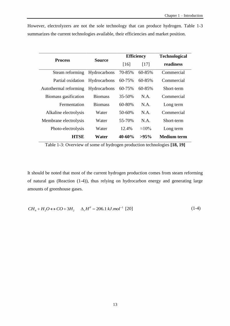
However, electrolyzers are not the sole technology that can produce hydrogen. Table 1-3
summarizes the current technologies available, their efficiencies and market position.
Process Source Efficiency Technological
readiness [16] [17]
Steam reforming Hydrocarbons 70-85% 60-85% Commercial
Partial oxidation Hydrocarbons 60-75% 60-85% Commercial
Autothermal reforming Hydrocarbons 60-75% 60-85% Short-term
Biomass gasification Biomass 35-50% N.A. Commercial
Fermentation Biomass 60-80% N.A. Long term
Alkaline electrolysis Water 50-60% N.A. Commercial
Membrane electrolysis Water 55-70% N.A. Short-term
Photo-electrolysis Water 12.4% ≈10% Long term
HTSE Water 40-60% >95% Medium term
Table 1-3: Overview of some of hydrogen production technologies [18, 19]
It should be noted that most of the current hydrogen production comes from steam reforming
of natural gas (Reaction (1-4)), thus relying on hydrocarbon energy and generating large
amounts of greenhouse gases.
1
4 2 23 206.1 .rCH H O CO H H kJ mol [20] (1-4)
Chapter 1 – Introduction
14
1.3.1. High Temperature Steam Electrolysis
Solid oxide materials used in SOECs (commonly Yttria Stabilized Zirconia - YSZ) become
sufficiently conducting for ions at high temperatures (between 500-1000°C, usually 800°C).
These operating temperatures allow to operate without expensive catalyzers: nickel is mostly
used as high temperature (193 $.kg-1
) compared to, for instance, platinum (44.000 $.kg-1
) [21].
Moreover, like in Solid Oxide Fuel Cell (SOFC) mode, high temperatures promote the
efficiency of electrochemical reactions by increasing kinetic rates, resulting in higher
performances.
The High Temperature Steam Electrolysis (HTSE) consumes less electrical energy than
electrolysis at room temperature because of favorable thermodynamic conditions. Indeed,
energy demand is significantly lowered by the vaporization of water into steam. Moreover,
steam electrolysis is increasingly endothermic with temperature, i.e. the required electrical
power is reduced at high temperatures [22].
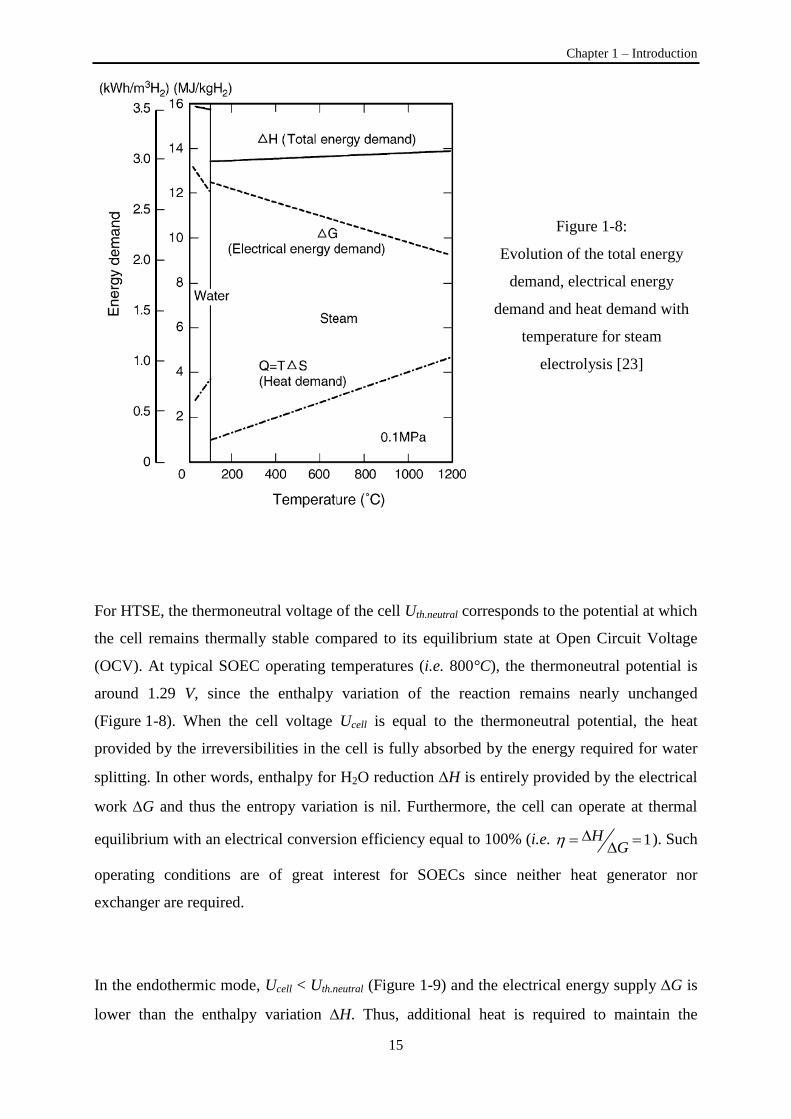
The electric energy required for the electrolysis process is equal to the variation of the Gibbs
free energy ΔG:
H T G T T S T (1-5)
where ΔH is the enthalpy variation of the water splitting reaction (1-3), T the absolute
temperature and ΔS the entropy variation.
A shown in Figure 1-8, the decrease in electrical energy ΔG is steeper than the increase in
total energy ΔH. Therefore, since heat is cheaper than electricity, electrolysis at high
temperatures reduces the cost of hydrogen production (3.1 kWh.Nm-3
H2 for HTSE compared
to 4.1 kWh.Nm-3
H2 at low temperatures [19]). This is especially the case if the heat energy
(TΔS) is supplied by an external heat source, such as nuclear power or renewable energy.
Chapter 1 – Introduction
15
Figure 1-8:
Evolution of the total energy
demand, electrical energy
demand and heat demand with
temperature for steam
electrolysis [23]
For HTSE, the thermoneutral voltage of the cell Uth.neutral corresponds to the potential at which
the cell remains thermally stable compared to its equilibrium state at Open Circuit Voltage
(OCV). At typical SOEC operating temperatures (i.e. 800°C), the thermoneutral potential is
around 1.29 V, since the enthalpy variation of the reaction remains nearly unchanged
(Figure 1-8). When the cell voltage Ucell is equal to the thermoneutral potential, the heat
provided by the irreversibilities in the cell is fully absorbed by the energy required for water
splitting. In other words, enthalpy for H2O reduction H is entirely provided by the electrical
work G and thus the entropy variation is nil. Furthermore, the cell can operate at thermal
equilibrium with an electrical conversion efficiency equal to 100% (i.e. 1HG
). Such
operating conditions are of great interest for SOECs since neither heat generator nor
exchanger are required.
In the endothermic mode, Ucell < Uth.neutral (Figure 1-9) and the electrical energy supply G is
lower than the enthalpy variation H. Thus, additional heat is required to maintain the

Chapter 1 – Introduction
16
operating temperature. In this mode, electrical conversion efficiency is higher than 100% [24]
(i.e. 1HG
). If heat is provided at a temperature higher than the cell temperature, the
mode is called allothermic.
When Ucell > Uth.neutral, the cell operates in the exothermic mode. It corresponds to an increase
of the cell temperature because the electric energy supply G exceeds the enthalpy variation
H. In this mode, the electrical conversion efficiency is lower than 100% ( 1HG
).
Figure 1-9:
Temperature of an
operating SRU -
thermal operating
modes for steam
electrolysis [25].
Regardless of the operating mode, performances of a solid oxide cell (SOC) in specific
conditions (composition of the gaseous inlet, temperature, etc.) are usually measured through
polarization curves, corresponding to the evolution of the cell voltage as a function of the cell
current density. By convention, and contrary to the SOFC mode where electricity is produced,
the current density supplied to a SOEC is negative. Typical polarization curves in both
operating modes are displayed in upcoming Figure 1-11.
The highest efficiencies displayed by SOCs are not their only advantage compared to other
electrolysis technologies. Due to a wide fuel flexibility with their ability to operate with
carbonated fuel such as natural gas, these systems have received a lot of attention these last
decades. Indeed, SOCs are able to oxidize or produce CO [26, 27], whereas CO is usually
considered as a poison for fuel cells operating at low temperature [28–30].
Tem
per
ature
(°C
)
Ucell=1500mV
Ucell=1300mV
Ucell=1100mV
Exothermic zoneEndothermic zone
Ucell=1400mV
Ucell=1200mV
Absolute current density (A cm-2)
Thermoneutral voltage
Chapter 1 – Introduction
17
1.3.2. High Temperature Carbone Dioxide Electrolysis
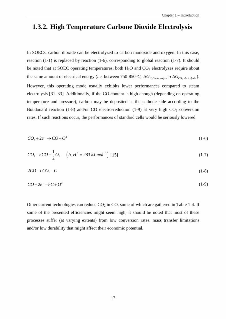
In SOECs, carbon dioxide can be electrolyzed to carbon monoxide and oxygen. In this case,
reaction (1-1) is replaced by reaction (1-6), corresponding to global reaction (1-7). It should
be noted that at SOEC operating temperatures, both H2O and CO2 electrolyzes require about
the same amount of electrical energy (i.e. between 750-850°C, 2 2 H O electrolysis CO electrolysisG G ).
However, this operating mode usually exhibits lower performances compared to steam
electrolysis [31–33]. Additionally, if the CO content is high enough (depending on operating
temperature and pressure), carbon may be deposited at the cathode side according to the
Boudouard reaction (1-8) and/or CO electro-reduction (1-9) at very high CO2 conversion
rates. If such reactions occur, the performances of standard cells would be seriously lowered.
2
2 2CO e CO O (1-6)
1
2 2
1 283 .
2rCO CO O H kJ mol
[15] (1-7)
22CO CO C (1-8)
22CO e C O (1-9)
Other current technologies can reduce CO2 in CO, some of which are gathered in Table 1-4. If
some of the presented efficiencies might seem high, it should be noted that most of these
processes suffer (at varying extents) from low conversion rates, mass transfer limitations
and/or low durability that might affect their economic potential.
Chapter 1 – Introduction
18
In addition and contrary to H2, CO is rarely if ever the desired end product. Consequently,
many processes, which are out of the scope of this work, have been developed to convert CO2
directly into a variety of fuels (e.g. methanol, methane, etc.). Therefore, Table 1-4 is not
intended to reflect the current state of the art in CO2 utilization.
Process Efficiency Ref.
Thermolysis 5-50% [34]
Thermochemical cycle 16-25% [35]
Alkaline Electrolysis 80% [36]
Molten carbonate electrolysis 80-90% [37]
HT electrolysis >100% *
Table 1-4: Overview of some of the technologies of production of CO from CO2 [38].
* if the required additional heat is supplied by an external cheap source. Electrolysis efficiency
is usually defined as the ratio of thermoneutral voltage to the operating voltage.
1.3.3. High Temperature H2O and CO2 Co-Electrolysis
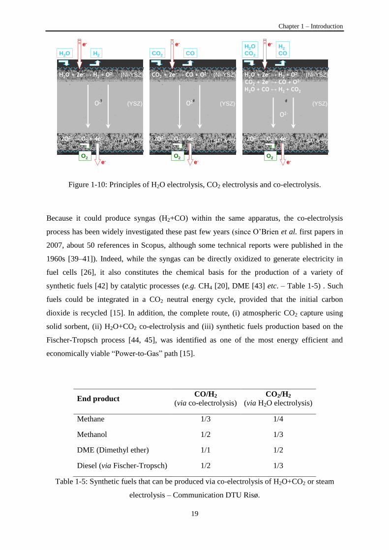
Weissbart et al. [39] first showed in 1967 that by adding CO2 to steam at the cell inlet, both
H2 and CO can be produced within a SOEC. In this co-electrolysis mode, both reactions (1-1)
and (1-7) could occur simultaneously. Furthermore, the Water Gas Shift (WGS) reaction (1-
10) may also take place at the cathode side. The elementary chemical reactions and transport
processes for single electrolyses and co-electrolysis of steam and carbon dioxide are shown in
Figure 1-10.
1
2 2 2 800 ,1 41 .rCO H O CO H H C atm kJ mol [20] (1-10)
Chapter 1 – Introduction
19
Figure 1-10: Principles of H2O electrolysis, CO2 electrolysis and co-electrolysis.
Because it could produce syngas (H2+CO) within the same apparatus, the co-electrolysis
process has been widely investigated these past few years (since O’Brien et al. first papers in
2007, about 50 references in Scopus, although some technical reports were published in the
1960s [39–41]). Indeed, while the syngas can be directly oxidized to generate electricity in
fuel cells [26], it also constitutes the chemical basis for the production of a variety of
synthetic fuels [42] by catalytic processes (e.g. CH4 [20], DME [43] etc. – Table 1-5) . Such
fuels could be integrated in a CO2 neutral energy cycle, provided that the initial carbon
dioxide is recycled [15]. In addition, the complete route, (i) atmospheric CO2 capture using
solid sorbent, (ii) H2O+CO2 co-electrolysis and (iii) synthetic fuels production based on the
Fischer-Tropsch process [44, 45], was identified as one of the most energy efficient and
economically viable “Power-to-Gas” path [15].
End product CO/H2
(via co-electrolysis)
CO2/H2
(via H2O electrolysis)
Methane 1/3 1/4
Methanol 1/2 1/3
DME (Dimethyl ether) 1/1 1/2
Diesel (via Fischer-Tropsch) 1/2 1/3
Table 1-5: Synthetic fuels that can be produced via co-electrolysis of H2O+CO2 or steam
electrolysis – Communication DTU Risø.
O2-
2O2- → O2 + 4e-
H2O + 2e-→ H2 + O2- (Ni-YSZ)
(YSZ)
(LSM-YSZ)
H2O H2
O2
e-
e-
O2-
2O2- → O2 + 4e-
CO2 + 2e- → CO + O2- (Ni-YSZ)
(YSZ)
(LSM-YSZ)
CO2 CO
O2
e-
e-
O2-
2O2- → O2 + 4e-
H2O + 2e-→ H2 + O2- (Ni-YSZ)
(YSZ)
(LSM-YSZ)
H2O
CO2
H2
CO
O2
e-
e-
CO2 + 2e- → CO + O2-
H2O + CO ↔ H2 + CO2
Chapter 1 – Introduction
20
By ultimately producing substitute natural gas, co-electrolysis could also provide an
environmentally friendly electricity storage option on a large scale (cf. Figure 1-5), that could
be implemented without adapting the current natural gas distribution network. Although
methane, the main component of natural gas, is usually produced through CO2 methanation
reaction (1-11), it can be alternately synthetized through CO methanation reaction (1-12).
This last chemical reaction makes a more efficient use of H2 in yielding CH4 compared to
CO2 methanation. Furthermore, CO hydrogenates more easily than CO2 [46]. Therefore, in
methane production scenario, syngas produced by co-electrolysis appears advantageous.
Nevertheless, it is worth noting that the thermal management of the highly exothermic CO
methanation reaction is hardened compared to its counterpart, and the methanator is more
likely to suffer from carbon deposition due to a lower oxygen content in the gas stream
(Figure 2-1).
1
2 2 4 24 2 165.0 .rCO H CH H O H kJ mol [46] (1-11)
1
2 4 23 206.1 .rCO H CH H O H kJ mol [46] (1-12)
However, since the regain of interest in H2O and CO2 high temperature co-electrolysis is as
recent as 2005, there is still much to be learned and understood. Indeed, the co-electrolysis
process is much more complicated than single electrolysis mechanisms. In addition, there is
currently no consensus concerning the electrochemical mechanism, and it is not clear whether
the reverse WGS reaction contributes to CO production [47, 48].
Chapter 1 – Introduction
21
1.4. Overview of a Solid Oxide Electrolysis Cell
There are many different physical phenomena occurring in a high temperature (co-)
electrolyzer. This section strives to explicit each one of them. The complete associated
mathematic equations will be detailed in Chapter 3.
1.4.1. Steady State
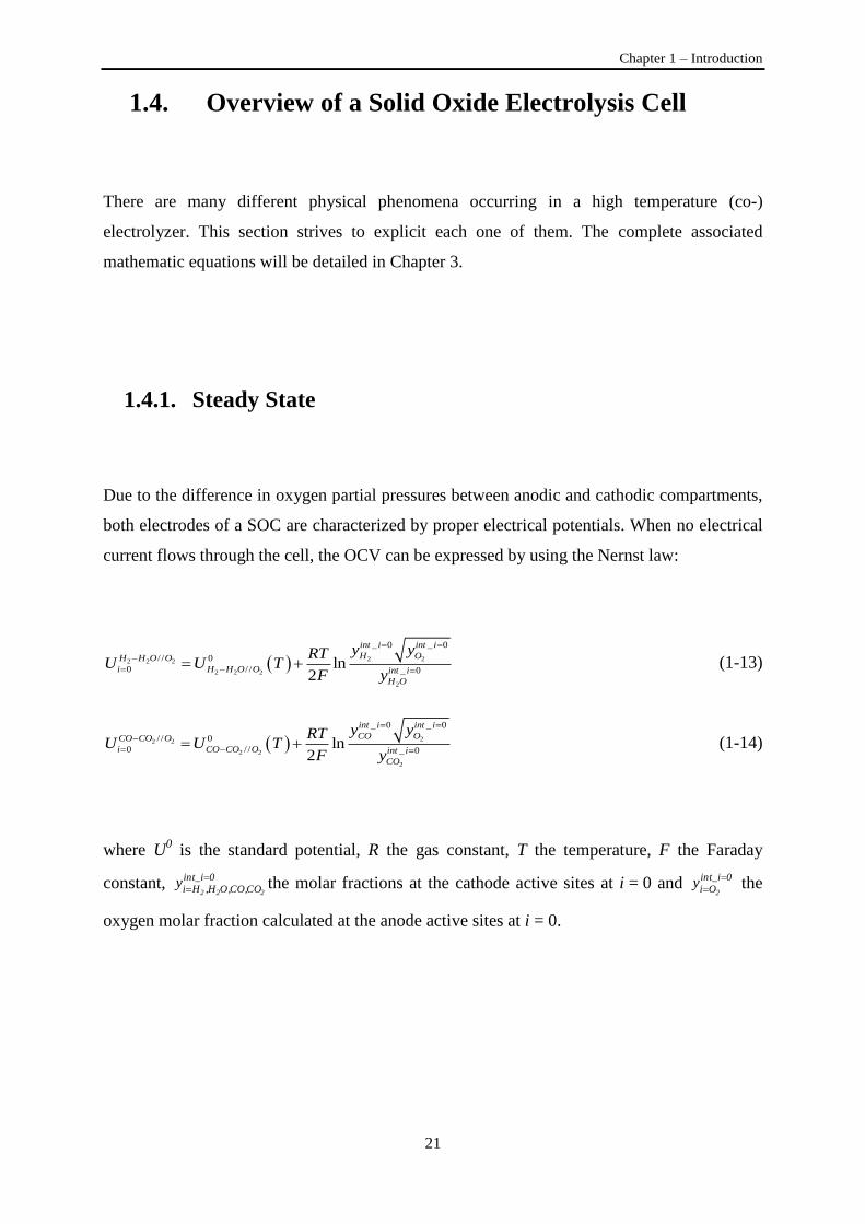
Due to the difference in oxygen partial pressures between anodic and cathodic compartments,
both electrodes of a SOC are characterized by proper electrical potentials. When no electrical
current flows through the cell, the OCV can be expressed by using the Nernst law:
2 22 2 2
2 2 2
2
_ 0 _ 0
/ / 0
0 / / _ 0ln
2
int i int i
H OH H O O
i H H O O int i
H O
y yRTU U T
F y
(1-13)
22 2
2 2
2
_ 0 _ 0
/ / 0
0 / / _ 0ln
2
int i int i
CO OCO CO O
i CO CO O int i
CO
y yRTU U T
F y
(1-14)
where U0 is the standard potential, R the gas constant, T the temperature, F the Faraday
constant, the molar fractions at the cathode active sites at i = 0 and the
oxygen molar fraction calculated at the anode active sites at i = 0.
0iint_
CO,CO,OH,Hi 222y
0iint_
Oi 2y
Chapter 1 – Introduction
22
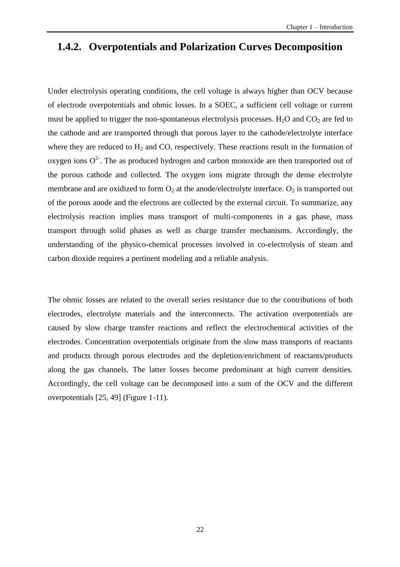
1.4.2. Overpotentials and Polarization Curves Decomposition
Under electrolysis operating conditions, the cell voltage is always higher than OCV because
of electrode overpotentials and ohmic losses. In a SOEC, a sufficient cell voltage or current
must be applied to trigger the non-spontaneous electrolysis processes. H2O and CO2 are fed to
the cathode and are transported through that porous layer to the cathode/electrolyte interface
where they are reduced to H2 and CO, respectively. These reactions result in the formation of
oxygen ions O2-
. The as produced hydrogen and carbon monoxide are then transported out of
the porous cathode and collected. The oxygen ions migrate through the dense electrolyte
membrane and are oxidized to form O2 at the anode/electrolyte interface. O2 is transported out
of the porous anode and the electrons are collected by the external circuit. To summarize, any
electrolysis reaction implies mass transport of multi-components in a gas phase, mass
transport through solid phases as well as charge transfer mechanisms. Accordingly, the
understanding of the physico-chemical processes involved in co-electrolysis of steam and
carbon dioxide requires a pertinent modeling and a reliable analysis.
The ohmic losses are related to the overall series resistance due to the contributions of both
electrodes, electrolyte materials and the interconnects. The activation overpotentials are
caused by slow charge transfer reactions and reflect the electrochemical activities of the
electrodes. Concentration overpotentials originate from the slow mass transports of reactants
and products through porous electrodes and the depletion/enrichment of reactants/products
along the gas channels. The latter losses become predominant at high current densities.
Accordingly, the cell voltage can be decomposed into a sum of the OCV and the different
overpotentials [25, 49] (Figure 1-11).
Chapter 1 – Introduction
23
For steam electrolysis, the cell voltage can be written:
2 2 2
2 2 2 2 2 2 2 2 2 2 2 2
/ /
0, , / / , / / , / / , / /
H H O O anode cathode anode cathode
cell i OCV ohm cell act H H O O act H H O O conc H H O O conc H H O OU U R i
(1-15)
where Rohm is the cell ohmic Area Specific Resistance (ASR), i the current density, ηact the
activation overpotentials and ηconc the concentration overpotentials.
The same type of expression prevails for carbon dioxide electrolysis:
2 2
2 2 2 2 2 2 2 2
/ /
0, , / / , / / , / / , / /
CO CO O anode cathode anode cathode
cell i OCV ohm cell act CO CO O act CO CO O conc CO CO O conc CO CO OU U R i
(1-16)
Figure 1-11: Typical decomposition of polarization curves in both SOFC and SOEC [19].
i-V curves can usually be decomposed into 3 zones: zone 1 is mainly governed by activation,
zone 2 by ohmic losses and zone 3 by mass transfer.
Due to mass transfer limitations, usually i lim HTE < i lim SOFC
i lim SOFC- i lim HTE
Chapter 1 – Introduction
24
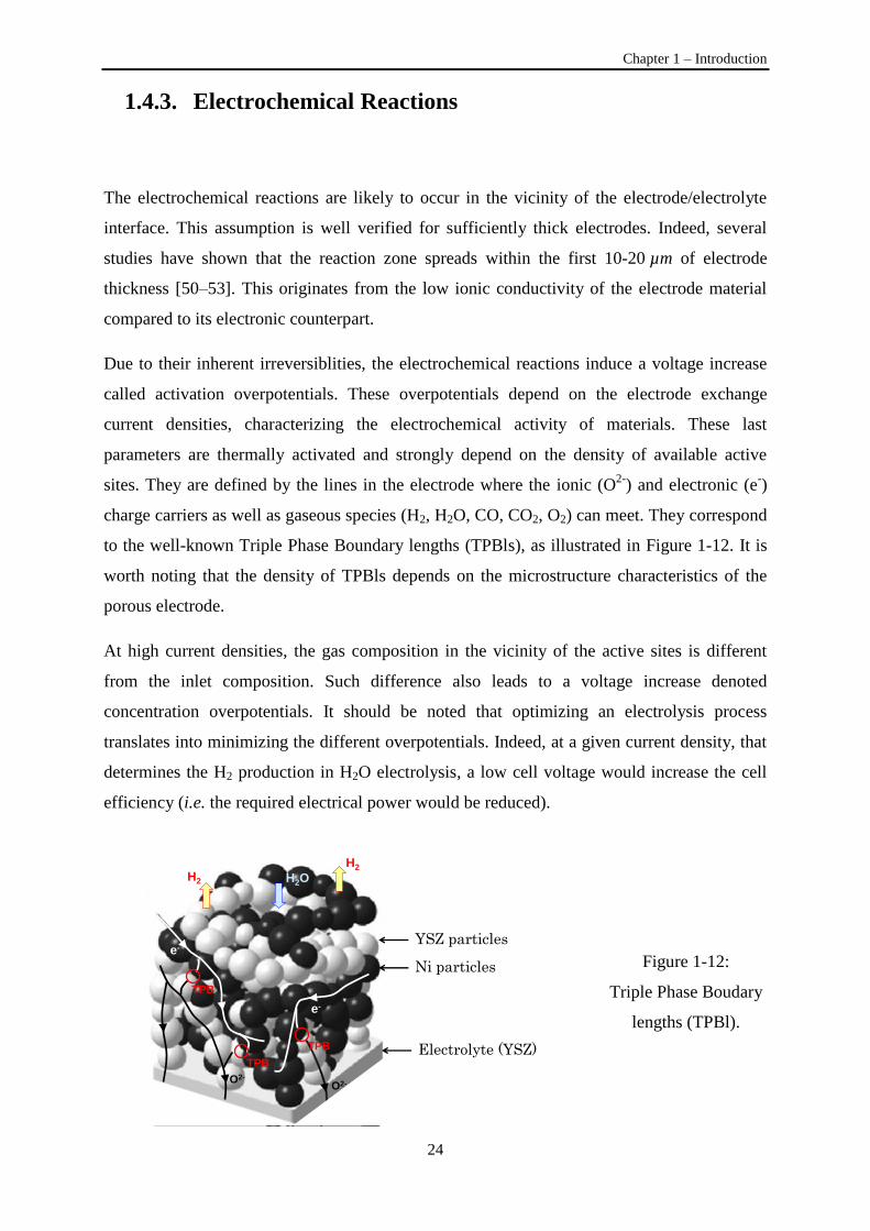
1.4.3. Electrochemical Reactions
The electrochemical reactions are likely to occur in the vicinity of the electrode/electrolyte
interface. This assumption is well verified for sufficiently thick electrodes. Indeed, several
studies have shown that the reaction zone spreads within the first 10-20 µm of electrode
thickness [50–53]. This originates from the low ionic conductivity of the electrode material
compared to its electronic counterpart.
Due to their inherent irreversiblities, the electrochemical reactions induce a voltage increase
called activation overpotentials. These overpotentials depend on the electrode exchange
current densities, characterizing the electrochemical activity of materials. These last
parameters are thermally activated and strongly depend on the density of available active
sites. They are defined by the lines in the electrode where the ionic (O2-
) and electronic (e-)
charge carriers as well as gaseous species (H2, H2O, CO, CO2, O2) can meet. They correspond
to the well-known Triple Phase Boundary lengths (TPBls), as illustrated in Figure 1-12. It is
worth noting that the density of TPBls depends on the microstructure characteristics of the
porous electrode.
At high current densities, the gas composition in the vicinity of the active sites is different
from the inlet composition. Such difference also leads to a voltage increase denoted
concentration overpotentials. It should be noted that optimizing an electrolysis process
translates into minimizing the different overpotentials. Indeed, at a given current density, that
determines the H2 production in H2O electrolysis, a low cell voltage would increase the cell
efficiency (i.e. the required electrical power would be reduced).
Figure 1-12:
Triple Phase Boudary
lengths (TPBl).
Electrolyte (YSZ)
Ni particles
YSZ particles
O2-O2-
e-
H2 H2O
H2
TPB
TPB
TPB
e-
Chapter 1 – Introduction
25
1.4.4. Mass Transport
For the sake of clarity, this section presents the mass transport phenomena in the specific case
of SOEC cathode (fuel electrode). Similar observations can be made at the anode side.
To reach the electroactive area in the vicinity of the cathode/electrolyte interface, gases of the
cathodic inlet stream first flow along the gas channel supplying reactants and collecting
products of the electrochemical reaction(s). Then, gases are transported through the porous
cathode to the electrolyte interface. The mass transfer is strongly dependent on the
microstructure properties. Diffusion of gases can be described by using three parameters: the
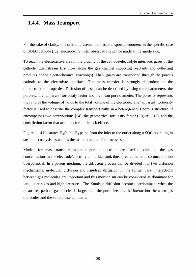
porosity, the ‘apparent’ tortuosity factor and the mean pore diameter. The porosity represents
the ratio of the volume of voids to the total volume of the electrode. The ‘apparent’ tortuosity
factor is used to describe the complex transport paths in a heterogeneous porous structure. It
encompasses two contributions [54]: the geometrical tortuosity factor (Figure 1-13), and the
constriction factor that accounts for bottleneck effects.
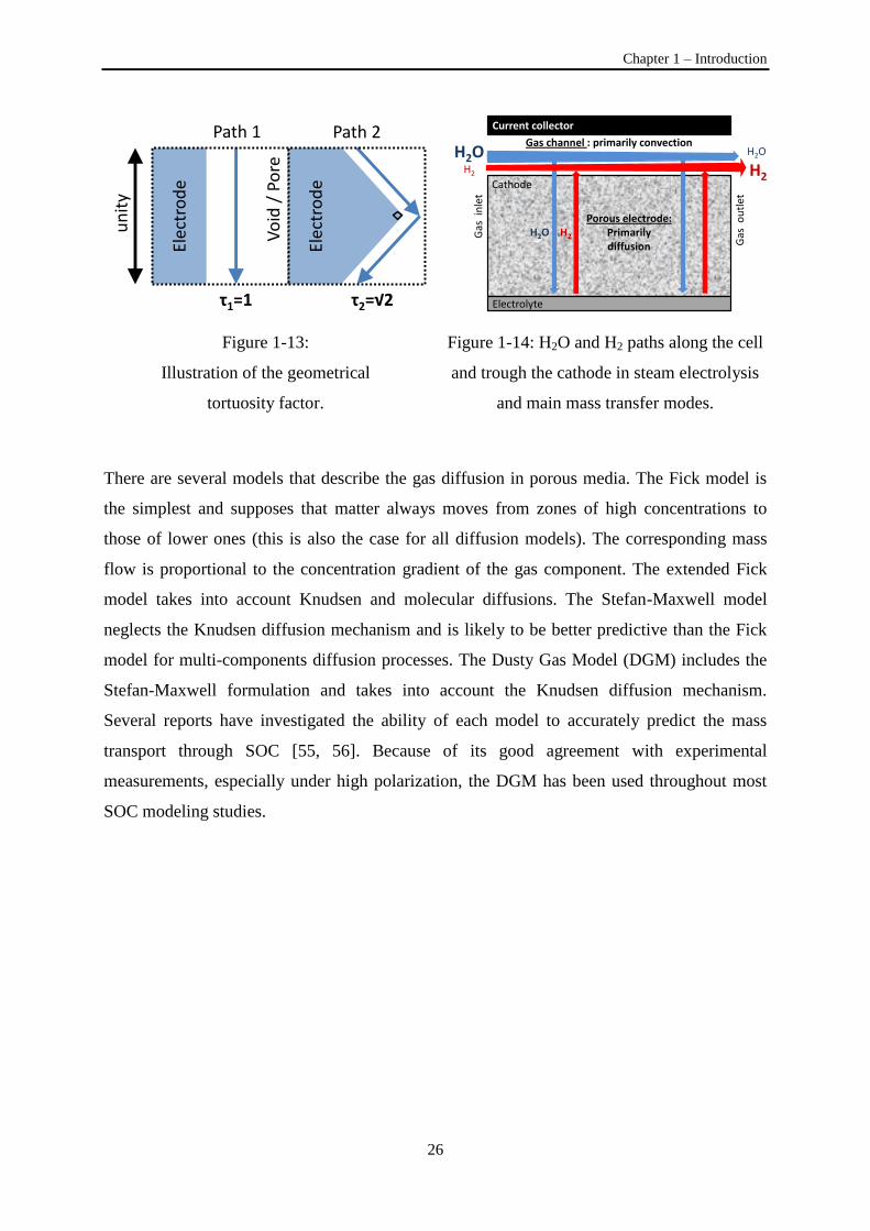
Figure 1-14 illustrates H2O and H2 paths from the inlet to the outlet along a SOC operating in
steam electrolysis, as well as the main mass transfer processes.
Models for mass transport inside a porous electrode are used to calculate the gas
concentrations at the electrode/electrolyte interface and, thus, predict the related concentration
overpotential. In a porous medium, the diffusion process can be divided into two diffusion
mechanisms: molecular diffusion and Knudsen diffusion. In the former case, interactions
between gas molecules are important and this mechanism can be considered as dominant for
large pore sizes and high pressures. The Knudsen diffusion becomes predominant when the
mean free path of gas species is larger than the pore size, i.e. the interactions between gas
molecules and the solid phase dominate.
Chapter 1 – Introduction
26
There are several models that describe the gas diffusion in porous media. The Fick model is
the simplest and supposes that matter always moves from zones of high concentrations to
those of lower ones (this is also the case for all diffusion models). The corresponding mass
flow is proportional to the concentration gradient of the gas component. The extended Fick
model takes into account Knudsen and molecular diffusions. The Stefan-Maxwell model
neglects the Knudsen diffusion mechanism and is likely to be better predictive than the Fick
model for multi-components diffusion processes. The Dusty Gas Model (DGM) includes the
Stefan-Maxwell formulation and takes into account the Knudsen diffusion mechanism.
Several reports have investigated the ability of each model to accurately predict the mass
transport through SOC [55, 56]. Because of its good agreement with experimental
measurements, especially under high polarization, the DGM has been used throughout most
SOC modeling studies.
Figure 1-13:
Illustration of the geometrical
tortuosity factor.
Figure 1-14: H2O and H2 paths along the cell
and trough the cathode in steam electrolysis
and main mass transfer modes.
Elec
tro
de
Path 1
Vo
id /
Po
re
un
ity
τ1=1El
ectr
od
eτ2=√2
Path 2 Current collector
Electrolyte
Cathode
H2O H2
Porous electrode: Primarilydiffusion
Gas channel : primarily convectionH2O
H2
H2O
H2
Gas
in
let
Gas
ou
tlet
Chapter 1 – Introduction
27
1.5. Objectives of the Study
This work aims at investigating the simultaneous co-electrolysis of H2O and CO2 at high
temperature, typically 800°C. Tackling this fairly new field of SOC application that was co-
electrolysis 3 years ago, this investigation should lead to the assessment of key outputs,
relevant for system design and technology evaluation. To do so, one must thus predict,
depending on operating conditions and cell materials and microstructure:
- cell performances (i.e. polarization curves),
- outlet composition,
- electrochemical and thermal behaviors in stack environments,
- operating maps.
Furthermore, as will be developed in the following chapter, a current lack of consensus exists
on co-electrolysis mechanism and on the relative influence of the WGS reaction over global
CO production. Thus, this work also aims at addressing these issues, through the
determination of respective influences of chemistry over electrochemistry, and the
formulation of a possible mechanism.
Finally, this study has provided scientific analysis of high temperature co-electrolysis in
French Research National Agency (ANR) project DEMETER (ANR-1-SEED-0005-01) and
European project MINERVE (KIC InnoEnergy, grant agreement 76_2012_IP35_MINERVE).
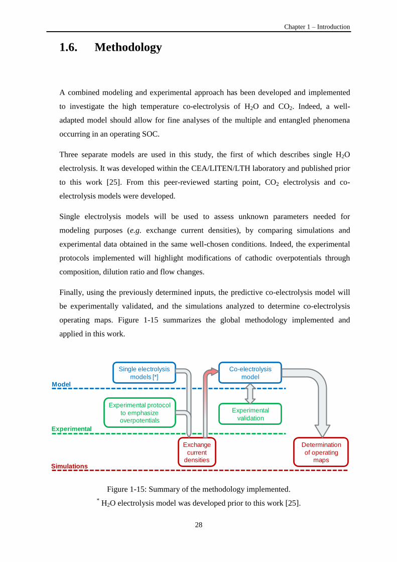
Chapter 1 – Introduction
28
1.6. Methodology
A combined modeling and experimental approach has been developed and implemented
to investigate the high temperature co-electrolysis of H2O and CO2. Indeed, a well-
adapted model should allow for fine analyses of the multiple and entangled phenomena
occurring in an operating SOC.
Three separate models are used in this study, the first of which describes single H2O
electrolysis. It was developed within the CEA/LITEN/LTH laboratory and published prior
to this work [25]. From this peer-reviewed starting point, CO2 electrolysis and co-
electrolysis models were developed.
Single electrolysis models will be used to assess unknown parameters needed for
modeling purposes (e.g. exchange current densities), by comparing simulations and
experimental data obtained in the same well-chosen conditions. Indeed, the experimental
protocols implemented will highlight modifications of cathodic overpotentials through
composition, dilution ratio and flow changes.
Finally, using the previously determined inputs, the predictive co-electrolysis model will
be experimentally validated, and the simulations analyzed to determine co-electrolysis
operating maps. Figure 1-15 summarizes the global methodology implemented and
applied in this work.
Figure 1-15: Summary of the methodology implemented.
* H2O electrolysis model was developed prior to this work [25].
Single electrolysis
models [*]
Experimental protocol
to emphasizeoverpotentials
Exchange
currentdensities
Co-electrolysis
model
Experimental
validation
Determination
of operating maps
Model
Experimental
Simulations
Chapter 1 – Introduction
29
1.7. References
1. J.-R. Petit, J. Jouzel, D. Raynaud, N. I. Barkov, J.-M. Barnola, I. Basile, M. Bender, J. Chappellaz,
M. Davis, and G. Delaygue, Climate and atmospheric history of the past 420,000 years from the
Vostok ice core, Antarctica, Nature 399, 429 (1999).
2. IPCC Fourth Assessment Report, Chapter 2, (2007).
3. http://www.acs.org/content/acs/en/climatescience/greenhousegases/industrialrevolution.html.
4. N. R. C. (US) C. on A. C. Choices, Advancing the Science of Climate Change: America’s Climate
Choices, National Academies Press (2010).
5. “World Bank. 2012. Turn Down the Heat: Why a 4°C Warmer World Must Be Avoided. ©
Washington, DC., (2012)
6. BP Statistical Review of World Energy, bp.com/statisticalreview (2012).
7. H. Iskov and N. B. Rasmussen, Global screening of projects and technologies for Power-to-Gas
and Bio-SNG,
http://www.dgc.dk/sites/default/files/filer/publikationer/R1307_screening_projects.pdf (2013)
8. M. Specht, U. Zuberbühler, F. Baumgart, B. Feigl, V. Frick, B. Stürmer, M. Sterner, and G.
Waldstein, Storing Renewable Energy in the Natural Gas Grid Methane via Power-to-Gas (P2G):
A Renewable Fuel for Mobility, (2011)
9. CEA, Energy Handbook, (2012).
10. G. Sandrock, A panoramic overview of hydrogen storage alloys from a gas reaction point of view,
J. Alloys Compd. 293, 877 (1999).
11. http://www.fuelcelltoday.com/about-fuel-cells/history.
12. A. Kirubakaran, S. Jain, and R. K. Nema, A review on fuel cell technologies and power electronic
interface, Renew. Sustain. Energy Rev. 13, 2430 (2009).
13. J. M. Andújar and F. Segura, Fuel cells: History and updating. A walk along two centuries,
Renew. Sustain. Energy Rev. 13, 2309 (2009).
14. A. B. Stambouli, Fuel cells: The expectations for an environmental-friendly and sustainable
source of energy, Renew. Sustain. Energy Rev. 15, 4507 (2011).
15. C. Graves, S. D. Ebbesen, M. Mogensen, and K. S. Lackner, Sustainable hydrocarbon fuels by
recycling CO2 and H2O with renewable or nuclear energy, Renew. Sustain. Energy Rev. 15, 1
(2011).
16. J. D. Holladay, J. Hu, D. L. King, and Y. Wang, An overview of hydrogen production
technologies, Catal. Today 139, 244 (2009).
17. A. Hauch, S. D. Ebbesen, S. H. Jensen, and M. Mogensen, Highly efficient high temperature
electrolysis, J. Mater. Chem. 18, 2331 (2008).
18. F. Chauveau, Synthèse et caractérisations électrochimiques de nouveaux matériaux pour anodes
d’électrolyseurs à haute température, (2009).
19. A. Mansuy, Etude de la durabilité de cellules d’électrolyse de la vapeur d’eau à haute
température: influence des paramètres de fonctionnement, (2012)
Chapter 1 – Introduction
30
20. J. Xu and G. F. Froment, Methane steam reforming, methanation and water-gas shift: I. Intrinsic
kinetics, AIChE J. 35, 88 (1989).
21. www.kitco.com (2013).
22. S. Dutta, Technology assessment of advanced electrolytic hydrogen production, Int. J. Hydrog.
Energy 15, 379 (1990).
23. R. Hino, K. Haga, H. Aita, and K. Sekita, 38. R&D on hydrogen production by high-
temperature electrolysis of steam, Nucl. Eng. Des. 233, 363 (2004).
24. J. E. O’Brien, Considerations for Thermal Water Splitting Processes and High Temperature
Electrolysis, Proc. 2008 Int. Mech. Eng. Congr. Expo. (2008)
25. J. Laurencin, D. Kane, G. Delette, J. Deseure, and F. Lefebvre-Joud, Modelling of solid oxide
steam electrolyser: Impact of the operating conditions on hydrogen production, J. Power Sources
196, 2080 (2011).
26. A. Weber, B. Sauer, A. C. Müller, D. Herbstritt, and E. Ivers-Tiffée, Oxidation of H2, CO and
methane in SOFCs with Ni/YSZ-cermet anodes, Solid State Ion. 152–153, 543 (2002).
27. W. Oser, Electrochemical method for conversion of carbon dioxide, Google Patents (1967).
28. J. J. Baschuk and X. Li, Carbon monoxide poisoning of proton exchange membrane fuel cells, Int.
J. Energy Res. 25, 695 (2001).
29. Q. Li, R. He, J.-A. Gao, J. O. Jensen, and N. J. Bjerrum, The CO Poisoning Effect in PEMFCs
Operational at Temperatures up to 200°C, J. Electrochem. Soc. 150, A1599 (2003).
30. J.-M. Le Canut, R. M. Abouatallah, and D. A. Harrington, Detection of Membrane Drying, Fuel
Cell Flooding, and Anode Catalyst Poisoning on PEMFC Stacks by Electrochemical Impedance
Spectroscopy, J. Electrochem. Soc. 153, A857 (2006).
31. P. Kim-Lohsoontorn, N. Laosiripojana, and J. Bae, Performance of solid oxide electrolysis cell
having bi-layered electrolyte during steam electrolysis and carbon dioxide electrolysis, Curr.
Appl. Phys. 11, S223 (2011).
32. J. E. O’Brien, M. G. McKellar, C. M. Stoots, J. S. Herring, and G. L. Hawkes, Parametric study of
large-scale production of syngas via high-temperature co-electrolysis, Int. J. Hydrog. Energy 34,
4216 (2009).
33. C. Graves, S. D. Ebbesen, and M. Mogensen, Co-electrolysis of CO2 and H2O in solid oxide
cells: Performance and durability, Solid State Ion. 192, 398 (2011).
34. A. J. Traynor and R. J. Jensen, Direct Solar Reduction of CO 2 to Fuel: First Prototype Results,
Ind. Eng. Chem. Res. 41, 1935 (2002).
35. A. Kogan, Direct solar thermal splitting of water and on-site separation of the products. III.
Improvement of reactor efficiency by steam entrainment, Int. J. Hydrog. Energy 25, 739 (2000).
36. H. Noda, S. Ikeda, Y. Oda, K. Imai, M. Maeda, and K. Ito, Electrochemical reduction of carbon
dioxide at various metal electrodes in aqueous potassium hydrogen carbonate solution., Bull.
Chem. Soc. Jpn. 63, 2459 (1990).
37. V. Kaplan, E. Wachtel, K. Gartsman, Y. Feldman, and I. Lubomirsky, Conversion of CO[sub 2] to
CO by Electrolysis of Molten Lithium Carbonate, J. Electrochem. Soc. 157, B552 (2010).
38. C. Graves, S. D. Ebbesen, M. Mogensen, and K. S. Lackner, Sustainable hydrocarbon fuels by
recycling CO2 and H2O with renewable or nuclear energy, Renew. Sustain. Energy Rev. 15, 1
(2011).
Chapter 1 – Introduction
31
39. J. Weissbart and W. Smart, Study of electrolytic dissociation of CO2-H2O using a solid oxide
electrolyte. NASA CR-680., NASA Contract. Rep. NASA CR U. S. Natl. Aeronaut. Space Adm. 1
(1967).
40. W. Smart and J. Weissbart, Development of a CO2-H2O Solid Oxide Electrolysis System : First
annual report, 29 March 1968–29 May 1969, Moffett Field, CA: National Aeronautics and Space
Administration, Ames Research Center (1969).
41. L. Elikan, J. Morris, and C. Wu, Development of a solid electrolyte carbon dioxide and water
reduction system for oxygen recovery, (1972).
42. I. Chorkendorff and J. W. Niemantsverdriet, Concepts of modern catalysis and kinetics, Wiley
(2003)
43. T. Ogawa, N. Inoue, T. Shikada, O. Inokoshi, and Y. Ohno, Direct Dimethyl Ether (DME)
synthesis from natural gas, J. Nat. Gas Chem. 22, 219 (2003).
44. M. E. Dry, The Fischer–Tropsch process: 1950–2000, Fisch.-Tropsch Synth. Eve XXI Century 71,
227 (2002).
45. W. L. Becker, R. J. Braun, M. Penev, and M. Melaina, Production of Fischer–Tropsch liquid fuels
from high temperature solid oxide co-electrolysis units, Energy 47, 99 (2012).
46. J. Gao, Y. Wang, Y. Ping, D. Hu, G. Xu, F. Gu, and F. Su, A thermodynamic analysis of
methanation reactions of carbon oxides for the production of synthetic natural gas, RSC Adv. 2,
2358 (2012).
47. C. Stoots, J. O’Brien, and J. Hartvigsen, Results of recent high temperature coelectrolysis studies
at the Idaho National Laboratory, Int. J. Hydrog. Energy 34, 4208 (2009).
48. M. Ni, An electrochemical model for syngas production by co-electrolysis of H2O and CO2, J.
Power Sources 202, 209 (2012).
49. J. Laurencin, F. Lefebvre-Joud, and G. Delette, Impact of cell design and operating conditions on
the performances of SOFC fuelled with methane, J. Power Sources 177, 355 (2008).
50. J.-W. Kim, Polarization Effects in Intermediate Temperature, Anode-Supported Solid Oxide Fuel
Cells, J. Electrochem. Soc. 146, 69 (1999).
51. S. B. Adler, Mechanism and kinetics of oxygen reduction on porous La1−xSrxCoO3−δ electrodes,
Solid State Ion. 111, 125 (1998).
52. S. Primdahl and M. Mogensen, Oxidation of hydrogen on Ni/yttria-stabilized zirconia cermet
anodes, J. Electrochem. Soc. 144, 3409 (1997).
53. E. Lay-Grindler, J. Laurencin, G. Delette, J. Aicart, M. Petitjean, and L. Dessemond, Micro
modelling of solid oxide electrolysis cell: From performance to durability, Int. J. Hydrog. Energy
38, 6917 (2013).
54. F. Usseglio-Viretta, J. Laurencin, G. Delette, J. Villanova, P. Cloetens, and D. Leguillon,
Quantitative microstructure characterization of a Ni–YSZ bi-layer coupled with simulated
electrode polarisation, J. Power Sources 256, 394 (2014).
55. R. Suwanwarangkul, E. Croiset, M. W. Fowler, P. L. Douglas, E. Entchev, and M. A. Douglas,
Performance comparison of Fick’s, dusty-gas and Stefan–Maxwell models to predict the
concentration overpotential of a SOFC anode, J. Power Sources 122, 9 (2003).
56. M. Andersson, J. Yuan, and B. Sundén, Review on modeling development for multiscale chemical
reactions coupled transport phenomena in solid oxide fuel cells, Appl. Energy 87, 1461 (2010).

Chapter 1 – Introduction
32

Chapter 2 – State of the Art
33
Chapter 2
State of the Art

Chapter 2 – State of the Art
34
Chapter 2 – State of the Art
35
Chapter 2
State of the Art
2.1. SOC Materials ..................................................................................................................... 36
2.1.1. Electrolyte .................................................................................................................... 37
2.1.2. Fuel Electrode .............................................................................................................. 38
2.1.3. Oxygen Electrode ........................................................................................................ 39
2.2. Recent Experimental Developments .................................................................................. 40
2.2.1. Performances ............................................................................................................... 40
2.2.2. Durability and Degradation........................................................................................ 43
2.2.2.1. Experimental Reports ......................................................................................... 43
2.2.2.2. Carbon Deposition ............................................................................................... 44
2.3. Modeling Studies ................................................................................................................. 45
2.4. References ............................................................................................................................ 47
Co-electrolysis studies are relying on decades of experimental developments of materials and
design optimization. Indeed, the high operating temperature yields rigorous and specific
constraints concerning the different components of an electrolyzer. It is worth mentioning that
specific materials have yet to be developed for the (co-)electrolysis mode. Indeed, the
materials currently used have been developed for high temperature fuel cell applications.
Regardless of the wealth of information that actual cell testing has represented throughout
several decades, the high temperature makes experimental works expensive and time
consuming. Indeed, because the cell housing, Single Repeating Units (SRU) or stacks have to
be maintained at around 800°C, it is quite more technical to equip the test bench with the
different sensors required for fine investigations than it would be for low temperature
Chapter 2 – State of the Art
36
systems. Additionally, SOC are complex devices to analyze due to the numerous physical
phenomena involved. Therefore, modeling approaches have been widely adopted to
investigate the multiphysics phenomena occurring inside a SOC. Experimental validation is
required to strengthen a model ability to predict the SOC behavior. It is worth noting that
most of these validations are performed by comparing experimental and simulated
polarization curves.
This chapter will first detail the most common materials utilized in a SRU operating in high
temperature electrolysis: electrolyte and electrodes materials. Then, experimental
developments in steam electrolysis, CO2 electrolysis and co-electrolysis will be overviewed.
A section focused on degradation mechanisms will also be presented. Finally, relevant
modeling studies of a SOEC operating in all electrolysis modes will be specified.
2.1. SOC Materials
The operating conditions for steam electrolysis or co-electrolysis induce high strains on the
materials constituting the SOEC, the SRU (cell coupled with two half interconnects) or the
stack (pileup of several SRUs). To be compatible with electrochemical processes, electrode
materials must foremost present sufficiently high electrical conductivities. For oxygen ion
conducting oxides, high ionic conductivities are reached above 600°C. Thus, the different
materials must exhibit compatible thermal expansion coefficients (TEC) along with good
thermal cyclability to withstand start and stop cycles [1–3]. Indeed, different TEC values
between adjacent cell layers induce mechanical stresses that can lead to cell failures.
Additionally, since both electrodes are in contact with highly oxidant/reducing atmospheres at
high temperature, electrodes and electrolyte should be chemically stable.
The main roles of the dense electrolyte membrane are to ensure the gas tightness between
both electrode compartments, to avoid any recombination of hydrogen and oxygen, and to
force the electrons in the outer circuit. Moreover, this membrane should be as thin as possible
to minimize the ohmic losses. Both electrodes should exhibit high electrocatalytic activity,
high ionic and electronic conductivities to promote the geometrical extent of the electrode
reactions from the electrolyte interface and to improve the current collection, respectively.
Chapter 2 – State of the Art
37
These electrodes should have suitable porosity to promote the matter transport in the gas
phase and provide sufficient reaction sites.
2.1.1. Electrolyte
The electrolyte is a key component in a SOC. Indeed, it must be an electronic insulator in a
wide range of oxygen partial pressure to avoid any short circuit reducing the current
efficiency. The most common electrolyte material is based on yttria doped zirconia. Since the
ohmic loss should be as low as possible for a given electrolyte thickness, the chosen ionic
conductor should exhibit the highest conductivity in the operating conditions. Accordingly,
scandia-doped zirconia (ScSZ) can be regarded as an interesting material, especially if one
refers to the results reported by the Idaho National Laboratory [4]. Indeed, this oxide exhibits
a higher ionic conductivity than yttria stabilized zirconia (YSZ), but its manufacturability
should be more expensive [5]. The stability of ScSZ remains also to be established since
thermal cycling of a cell results in an Area Specific Resistance (ASR) degradation [4].
Moreover, the ionic conductivity of ScSZ can hugely degrade during isothermal ageing in
SOFC mode at high temperatures [6]. If one refers strictly to the ionic conductivity value,
ceria-based oxides, doped either by Gd2O3 (GDC) or Sm2O3 (SDC), can be regarded as
promising electrolytes for electrolysis operation, at least for temperatures up to 700°C. The
use of SDC as an electrolyte was found effective in lowering both cathode and anode
overpotentials in an electrolysis mode [7]. But, the main problem is that cerium cations can be
partly reduced in a reducing atmosphere or fully reduced under high applied voltages. Despite
deteriorating the ionic transfer number, this reduction process could also lead to a mechanical
failure of a cell [8]. Recently, the use of a bi-layered GDC/YSZ electrolyte was proposed to
increase the performances compared to cells only involving YSZ or GDC [9]. But, as for
ScSZ, the stability of such an assembly in operating conditions must be investigated. LaGaO3
doped with strontium and magnesium (LSGM) could be used as an electrolyte for steam
electrolysis [10] because the ionic conductivity of LSGM is higher than that of YSZ.
However, the electronic conductivity of LSGM depends on its microstructure and thus on the
sintering conditions [11]. Moreover, LSGM is likely to react with a nickel containing
electrode to form additional phases [12], resulting in a loss of conductivity [13].
Chapter 2 – State of the Art
38
At this stage, taking into account the level of ionic conductivity, the chemical stability as well
as economic reasons, the most common electrolyte material for SOECs remains YSZ with
dopant contents between 3 and 10 mol.% [14]. Within a wide range of oxygen partial
pressure, the purely ionic conductivity of YSZ is of the order of 0.03 S.cm-1
at 700°C [15] and
0.2 S.cm-1
at 1000°C [5]. As can be seen in Table 2-1 which gathers performances and
degradation reports, high performances as well as low degradation rates can be obtained using
cells based on YSZ. This observation is probably related to the fact that YSZ is the most
commonly optimized (in terms of elaboration, microstructure, etc.) and tested material.
2.1.2. Fuel Electrode
The oxygen partial pressure at the cathode side of a SOEC is expected to vary between 10-12
and 10-16
atm. Therefore, materials like nickel and cobalt can be used [16]. Although Ni
exhibits a high electrochemical activity for the oxidations of hydrogen and carbon monoxide,
it is only an electronic conductor. Thus, the nickel particles must be mixed with an ion
conducting material, the same material than the electrolyte such as YSZ, in order to increase
the number of active sites. The addition of a ceramic material also allows to limit the
coarsening of nickel particles and to adapt the TEC of the electrode to that of the electrolyte.
Nevertheless, the electrode must be porous (porosity varying between 30 and 50 vol.%) to
support the diffusion of steam (and/or carbon dioxide) and hydrogen (and/or carbon
monoxide) during high temperature electrolysis. Depending on the elaboration conditions of
the cermet Ni-YSZ, effective electronic conductivities as high as 800-1200 S.cm-1
can be
reached at 800°C [17], allowing an efficient collection of electrons in operating conditions.
Accordingly, the cermet Ni-YSZ is presently the cathode material widely used in SOECs [10,
14], as shown in Table 2-1. In order to avoid the reoxidation of Ni to NiO, which can result in
a mechanical failure of the cermet layer [18–20], small amounts of hydrogen are required at
the cathode side (during operating steps without polarization, i.e. without H2 production).
Furthermore, some studies have reported on the degradation of the Ni-YSZ cermet during
long-term wet conditions [21–23] . This is accompanied by a coarsening of the Ni particles in
the cermet yielding a decrease in density of active sites (TPBls) [24].
Chapter 2 – State of the Art
39
It is worth mentioning that only few studies have been devoted to the use of new cathode
materials in H2O (and/or CO2) electrolysis applications. The electrochemical behavior of
mixed conducting Ni-SDC was evaluated [25]. The results of Marina et al. [26] suggest that
strontium-doped lanthanum titanate-ceria composites seem to be more active than Ni-YSZ.
Recently, La0.75Sr0.25Cr0.5Mn0.5O3 (LSCM) has been proposed as an alternative cathode
material for steam electrolysis [27]. However, the current collection must be improved since
the effective conductivity is low in reducing environments.
2.1.3. Oxygen Electrode
In SOEC mode, the oxygen electrode operates in a highly oxidizing atmosphere. Accordingly,
only conducting oxides are suitable materials for such an electrode. Strontium-doped
lanthanum manganite La1-xSrxMnO3 (LSM) is the oldest electrode material commercially used
for SOFCs. In order to increase the number of active sites for the oxidation of oxygen ions,
LSM is mixed with the electrolyte material and the most common material for an oxygen
electrode is the composite LSM-YSZ [28–30]. Note that the TEC of LSM is close to that of
YSZ, thus ensuring the integrity of the cell. Moreover, the chemical reactivity between LSM
and YSZ is rather low especially at high O2 partial pressure and this should extend the
lifetime during operation.
Despite a good stability, LSM-based anodes may not appear optimal for high temperature
electrolysis [31]. Thus, alternative materials for oxygen electrodes have been proposed over
the past few years, including mixed ionic and electronic conductors (MIECs), like strontium-
doped lanthanum ferrite (LSF) [32], strontium-doped lanthanum copper-ferrite (LSCuF) [10],
strontium-doped lanthanum cobalt-ferrite (LSCoF) [33], strontium-doped lanthanum cobaltite
(LSC) [34] and more recently strontium-doped barium cobalt-ferrite (BSCF) [35]. Among
these materials, strontium-doped lanthanum cobaltite (LSC) and strontium-doped lanthanum
cobalt-ferrite (LSCF) present lower polarization losses than LSM by operating as an SOEC
anode [32, 36–38]. The performances of BSCF decrease during high temperature electrolysis
because of a change in microstructure. The chemical stability of BSCF must be improved and
durability studies must be performed prior to any application as a SOEC anode. Solid state
reactions have been evidenced between LSC (LSCF) and YSZ, resulting in lower cell
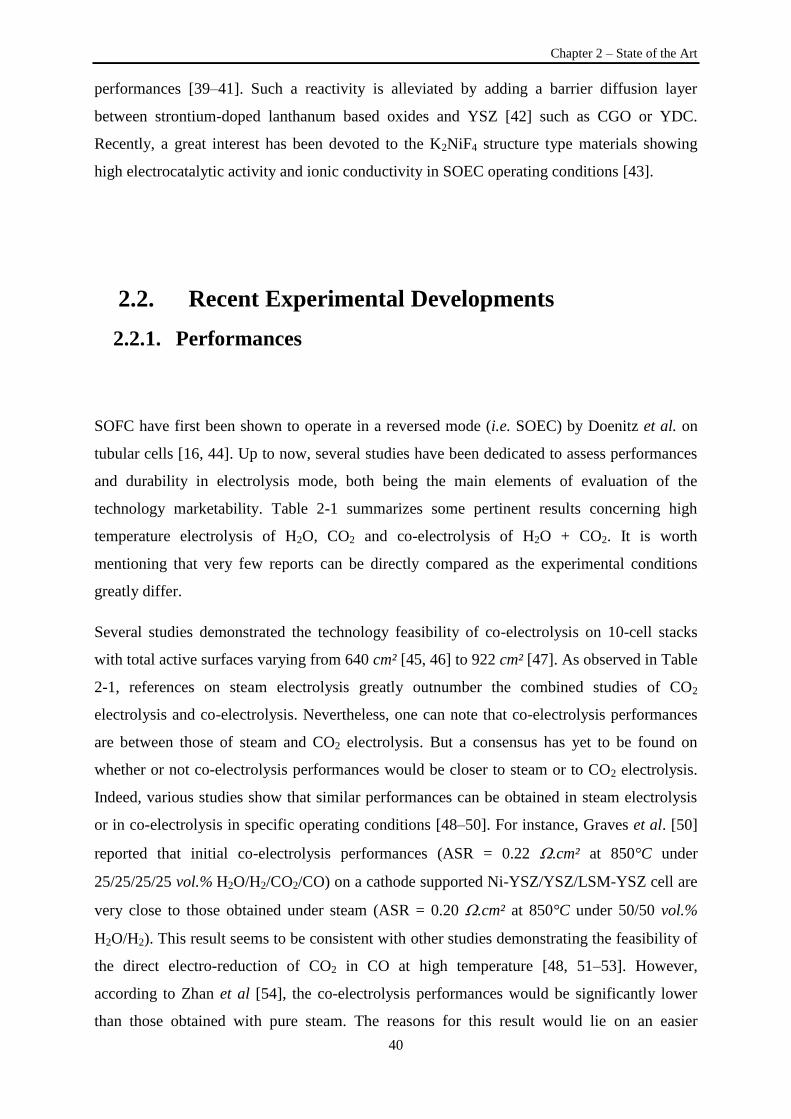
Chapter 2 – State of the Art
40
performances [39–41]. Such a reactivity is alleviated by adding a barrier diffusion layer
between strontium-doped lanthanum based oxides and YSZ [42] such as CGO or YDC.
Recently, a great interest has been devoted to the K2NiF4 structure type materials showing
high electrocatalytic activity and ionic conductivity in SOEC operating conditions [43].
2.2. Recent Experimental Developments
2.2.1. Performances
SOFC have first been shown to operate in a reversed mode (i.e. SOEC) by Doenitz et al. on
tubular cells [16, 44]. Up to now, several studies have been dedicated to assess performances
and durability in electrolysis mode, both being the main elements of evaluation of the
technology marketability. Table 2-1 summarizes some pertinent results concerning high
temperature electrolysis of H2O, CO2 and co-electrolysis of H2O + CO2. It is worth
mentioning that very few reports can be directly compared as the experimental conditions
greatly differ.
Several studies demonstrated the technology feasibility of co-electrolysis on 10-cell stacks
with total active surfaces varying from 640 cm² [45, 46] to 922 cm² [47]. As observed in Table
2-1, references on steam electrolysis greatly outnumber the combined studies of CO2
electrolysis and co-electrolysis. Nevertheless, one can note that co-electrolysis performances
are between those of steam and CO2 electrolysis. But a consensus has yet to be found on
whether or not co-electrolysis performances would be closer to steam or to CO2 electrolysis.
Indeed, various studies show that similar performances can be obtained in steam electrolysis
or in co-electrolysis in specific operating conditions [48–50]. For instance, Graves et al. [50]
reported that initial co-electrolysis performances (ASR = 0.22 .cm² at 850°C under
25/25/25/25 vol.% H2O/H2/CO2/CO) on a cathode supported Ni-YSZ/YSZ/LSM-YSZ cell are
very close to those obtained under steam (ASR = 0.20 .cm² at 850°C under 50/50 vol.%
H2O/H2). This result seems to be consistent with other studies demonstrating the feasibility of
the direct electro-reduction of CO2 in CO at high temperature [48, 51–53]. However,
according to Zhan et al [54], the co-electrolysis performances would be significantly lower
than those obtained with pure steam. The reasons for this result would lie on an easier

Chapter 2 – State of the Art
41
diffusion process of H2/H2O compared to CO/CO2 in a porous electrode and on a faster
charge transfer for the steam reduction.
Nevertheless, only limited understanding and knowledge are available on the co-electrolysis
elementary mechanisms. For instance, the amounts of CO produced by co-electrolysis and by
the reverse WGS reaction would strongly depend on operating conditions (temperature,
operating voltage, H2O/CO2 inlet ratio, etc.) [55].
Chapter 2 – State of the Art
42
Cell electrodes and thicknesses Active area
Mode
T Composition Flow Performances* Degradation
Ref. Fuel electrode Electrolyte O2 electrode Cells Sone cell Stot NmL.
min-1cm-²
i(0) U(1) i SC(2) time deg.
Material µm Material µm Material µm Nb. cm² cm² °C %volume A/cm² V A/cm² % h %U.kh-1
Ni-YSZ 400+10(3) 8YSZ 10 LSM-YSZ 30-40 30 10×10 3.000 H2O elec. 800 80/20 H2O/H2 -0.3 1.58 -0.15 62 1100 11.7 [56]
Ni-YSZ 1500 8YSZ 10 CGO/LSCF 5+40 1 Ø7.6 45 H2O elec. 772 80/9.2/10.8 H2O/H2/N2 24.2 -1.5 1.2 -1 36 9300 3.8 [57]
Ni-YSZ 1500(4) YSZ LSCF 2 80 160
SOFC 750 18/82 H2O/H2 10.6 +0.5 40 3820 -0.6
[58] H2O elec. 810 50/50 H2O/H2 27.5 -0.8 1.2 -0.3 15 2034 -0.2
Co-elec. 760 25/25/50 H2O/CO2/H2 27.5 -0.3 15 174 1.0
Ni-YSZ/ScSZ 680+15(3) ScSZ 20 LSM-ScSZ 15 1 Ø1.3 1.33 CO2 elec. 750 50/50 CO2/CO 226 -0.3 1.4 [59]
Ni-YSZ/ScSZ 680+15(3) ScSZ 20 LSM-ScSZ 15 1 Ø1.3 1.33 Co-elec. 750 29/29/14/29 H2O/CO2/H2/Ar 263 -0.43 1.35 [60]
Ni-YSZ 300+15(3) YSZ 15 LSM-YSZ 20 1 4×4 16
H2O elec.
850
50/50 H2O/H2
26
-1.15 1.25
[50]
Co-elec. 25/25/25/25 H2O/CO2/H2/CO -1 1.25
CO2 elec. 50/50 CO2/CO -0.85 1.25
Co-elec. 45/45/10 H2O/CO2/H2 -0.5 15 200 0.1mV.h-1
-1 30 200 1mV.h-1
Ni-YSZ 300+15(3) YSZ 15 LSM-YSZ 20 1 4×4 16
H2O elec.
850
50/25/25 H2O/H2/Ar -1.05 1.3
[61] Co-elec. 25/25/25/25 H2O/CO2/CO/Ar -0.90 1.3
CO2 elec. 50/25/25 CO2/CO/Ar -0.84 1.3
Ni-YSZ YSZ 150(5) LSM 10 8×8 640
H2O elec. 800 55/22.5/22.5 H2O/H2/N2 3.13
-0.35 1.35
[45] Co-elec. 800 55/22.5/22.5 H2O/CO2/N2 -0.35 1.35
CO2 elec. 800 100 CO2 2.34 -0.12 1.3
Ni-YSZ YSZ LSM-YSZ 10 9.6×9.6 922
H2O elec. 850 50/50 H2O/H2 20 -0.25 1.05 -0.25 17 900 250mV.kh-1
[47] Co-elec. 850 45/45/10 H2O/CO2/H2 6.5 -0.65 1.2
-0.5 60 800 190mV.kh-1
-0.75 60 350 100mV.kh-1
Table 2-1: Overview of some performances and degradations reports in recent literature
*: Performances taken at the maximum of a typical polarization curve
(0): In case of a stack, the indicated current density corresponds to the stack current divided by the active area of one cell
(1): In case of a stack, the indicated voltage corresponds to the stack voltage divided by the number of cell
(2): Steam conversion for steam electrolysis, CO2 conversion in CO2 electrolysis, H2 conversion in SOFC, global conversion (H2O+CO2) for co-electrolysis
(3): Functional layer (4): Total average cell thickness (5): Electrolyte supported cell
Chapter 2 – State of the Art
43
2.2.2. Durability and Degradation
2.2.2.1. Experimental Reports
There are large discrepancies in experimental conditions and degradation reports, regardless
of the operating mode (Table 2-1). Still, degradation rates experienced by cells operating in
co-electrolysis seem to be more severe than for steam electrolysis, as investigated by Nguyen
et al. [58]. These authors compared the voltage evolution of a two Ni-YSZ/YSZ/CGO/LSCF
cells stack operating in H2O electrolysis, CO2 electrolysis and co-electrolysis, and showed
that the voltage degradation is a bit higher in co-electrolysis compared to steam electrolysis.
At 760°C and 15% reactant utilization, degradations rates comprised between 0.5 and
1.5%.kh-1
for 50/50 vol.% H2/H2O steam electrolysis and between 1.0 and 6.1%.kh-1
(ΔU/U)
for 25/25/50 vol.% H2O/CO2/H2 co-electrolysis were recorded. Furthermore, whatever the
operating mode, degradation rates have been reported to level off after a few hundred hours of
operation [62, 47, 58].
It should be noted that some research groups have investigated performances and
degradations of cells fed with CO2+H2 inlet mixture [58]. However, it is unclear if such inlet
mixtures would lead to CO2 electrolysis or H2O electrolysis subsequent to the WGS reaction.
Most probably, the reality would lie somewhere between these two extremes. For that reason,
these reports are not included in Table 2-1 and this section.
Over long term measurements, cells operating in co-electrolysis should degrade following
some of the same mechanisms, if not all, than in steam electrolysis. Since the present work is
not focused on durability, the degradation mechanisms are not detailed here. The reader can
refer to references [10, 14, 63–65] for an overview on the most liable phenomena that could
drive the degradation in electrolysis performances.
Only a short report is presented in the next section on the risk of carbon deposition that arises
in the specific cases of CO2 or co-electrolysis operations.
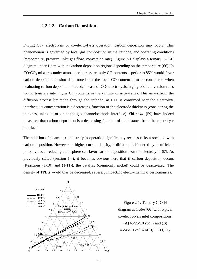
Chapter 2 – State of the Art
44
2.2.2.2. Carbon Deposition
During CO2 electrolysis or co-electrolysis operation, carbon deposition may occur. This
phenomenon is governed by local gas composition in the cathode, and operating conditions
(temperature, pressure, inlet gas flow, conversion rate). Figure 2-1 displays a ternary C-O-H
diagram under 1 atm with the carbon deposition regions depending on the temperature [66]. In
CO/CO2 mixtures under atmospheric pressure, only CO contents superior to 85% would favor
carbon deposition. It should be noted that the local CO content is to be considered when
evaluating carbon deposition. Indeed, in case of CO2 electrolysis, high global conversion rates
would translate into higher CO contents in the vicinity of active sites. This arises from the
diffusion process limitation through the cathode: as CO2 is consumed near the electrolyte
interface, its concentration is a decreasing function of the electrode thickness (considering the
thickness takes its origin at the gas channel/cathode interface). Shi et al. [59] have indeed
measured that carbon deposition is a decreasing function of the distance from the electrolyte
interface.
The addition of steam in co-electrolysis operation significantly reduces risks associated with
carbon deposition. However, at higher current density, if diffusion is hindered by insufficient
porosity, local reducing atmosphere can favor carbon deposition near the electrolyte [67]. As
previously stated (section 1.4), it becomes obvious here that if carbon deposition occurs
(Reactions (1-10) and (1-11)), the catalyst (commonly nickel) could be deactivated. The
density of TPBls would thus be decreased, severely impacting electrochemical performances.
Figure 2-1: Ternary C-O-H
diagram at 1 atm [66] with typical
co-electrolysis inlet compositions:
(A) 65/25/10 vol.% and (B)
45/45/10 vol.% of H2O/CO2/H2.
Carbon deposition
region
(%C(s) > 10-6
%C)
CH4
H2O
CO2
P = 1 atm
1000 °C
800 °C
750 °C
600 °C
400 °C
(%C(s) < 10-6
%C)
(A)
(B)
CO
Chapter 2 – State of the Art
45
2.3. Modeling Studies
Computational simulation appears to be one efficient approach to analyze the coupled
mechanisms of HTSE. Indeed, the cell response depends on entangled multi-physics
phenomena such as electrochemical reactions, as well as mass and energy transport in the
electrolyzer. Furthermore, all chemical and electrochemical source terms are linked to the
local temperature field throughout the SOEC. Steam electrolysis has been widely modeled
because this approach allows the identification of governing factors within the deeply
interconnected phenomena occurring inside a SOC. Conversely, very few studies have been
dedicated to the modeling of CO2 electrolysis and/or co-electrolysis of H2O and CO2. This
section aims at giving an overview of the published models. It should be noted that the
approach followed to simulate SOEC is usually very similar to the one used to investigate the
SOFC response.
Some models were recently developed to describe the HTSE. Ni et al. [55, 68] proposed
isothermal models taking into account the coupled mass transport and electrochemical
reactions. A 2D multi-physics in-house-model has been developed by Laurencin et al. [69] to
analyze the performances of a SRU or a stack. This model encompasses a combined
electrochemical and thermal description of the electrolyzer, where the mass transport through
the porous electrodes has been computed in the frame of the dusty-gas-model (DGM). More
recently, Udagawa et al. [70, 71] developed a one dimensional dynamic model including a
thermal analysis. A 2D in-house Computational Fluid Dynamic (CFD) model has been
proposed by Ni [72] for a better understanding of HTSE operation. This approach can serve
for design optimization and was extended to a 3D model [73, 74] by using a commercial CFD
software. Grondin et al. [75] developed a “local” model focused on the cathode response and
identified an electrochemical process that should be limited by the adsorption of water
molecules. Lay et al. [24] also developed a “local” anode model and the authors shown that
the kinetic response of a LSM-YSZ oxygen electrode could be controlled by a charge transfer
followed by an O2 desorption step.
In co-electrolysis mode, thermodynamic investigations have also been carried out on the
effect of temperature, pressure and inlet composition on the outlet gas and performances [58,
Chapter 2 – State of the Art
46
76]. Stoots et al. [45] have developed a chemical equilibrium co-electrolysis model to
determine the co-electrolyzer outlet composition. The simulations show remarkable
agreement with experimental CO, CO2 and H2 contents measured by gas analyses, up to the
maximum cell current density investigated of 0.24 A.cm-2
. After investigating CO2 electrolysis
[77], Ni et al. [55, 78] have recently developed a kinetic model taking into account the CO2
electro-reduction and the reverse water gas shift reaction. These authors have shown that the
WGS reaction can either produce or consume CO depending on the cell inlet gas stream
composition, cell temperature and operating voltage.
Furthermore, based on the initial work of Hecht et al. [79] in a SOFC mode, some recent
studies were focused on finding limiting elementary steps among extensive electrochemical
pathways concerning the co-electrolysis [80, 81] or CO2 electrolysis process [59]. It is worth
mentioning that all these studies assume that the reaction pathway in electrolysis anodic
polarization is the same than the one proposed in fuel cell cathodic polarization. The authors
proposed pathways respectively divided in 10 [59], 18 [80] and 21 [81] elementary reactions.
They calibrated their models on experimental polarization curves. Furthermore, Yurkiv et al.
[82] highlighted that CO oxidation on Ni-YSZ electrodes may be subjected to a change in
rate-determining step depending on CO partial pressure. Despite these findings, no clear
consensus seems to emerge concerning the co-electrolysis mechanisms.
Additionally, no consensus arises from the literature concerning the influence of the WGS
reaction on CO production in a co-electrolyzer. Indeed, several models are based on the
hypothesis that all CO is chemically produced through the reverse WGS reaction [45, 58, 83].
Conversely, Ni et al. [55] shown that the WGS reaction accounts for large shifts in CO
production, but that the electrochemical production remains preponderant. This lack of
agreement has led Sun et al. [76] to combine a fast and dominant WGS kinetics along with a
fixed electrochemical utilization for both H2O and CO2 when simulating a co-electrolyzer.
Chapter 2 – State of the Art
47
2.4. References
1. M. Mori, Thermal Expansion of Nickel-Zirconia Anodes in Solid Oxide Fuel Cells during Fabrication
and Operation, J. Electrochem. Soc. 145, 1374 (1998).
2. N. H. Menzler, F. Tietz, S. Uhlenbruck, H. P. Buchkremer, and D. Stöver, Materials and
manufacturing technologies for solid oxide fuel cells, J. Mater. Sci. 45, 3109 (2010).
3. C.-K. Lin, T.-T. Chen, Y.-P. Chyou, and L.-K. Chiang, Thermal stress analysis of a planar SOFC
stack, J. Power Sources 164, 238 (2007).
4. J. E. O’Brien, C. M. Stoots, J. S. Herring, and J. J. Hartvigsen, Performance of Planar High-
Temperature Electrolysis Stacks for Hydrogen Production from Nuclear Energy, Nucl. Technol. 158,
118 (2007).
5. M. Ni, M. K. H. Leung, and D. Y. C. Leung, Technological development of hydrogen production by
solid oxide electrolyzer cell (SOEC), Int. J. Hydrog. Energy 33, 2337 (2008).
6. C. Haering, A. Roosen, H. Schichl, and M. Schnoller, Degradation of the electrical conductivity in
stabilised zirconia systemPart II: Scandia-stabilised zirconia, Solid State Ion. 176, 261 (2005).
7. K. Eguchi, Power generation and steam electrolysis characteristics of an electrochemical cell with a
zirconia- or ceria-based electrolyte, Solid State Ion. 86-88, 1245 (1996).
8. V. Kharton, F. Marques, and A. Atkinson, Transport properties of solid oxide electrolyte ceramics: a
brief review, Solid State Ion. 174, 135 (2004).
9. P. Kim-Lohsoontorn, N. Laosiripojana, and J. Bae, Performance of solid oxide electrolysis cell having
bi-layered electrolyte during steam electrolysis and carbon dioxide electrolysis, Curr. Appl. Phys. 11,
S223 (2011).
10. M. A. Laguna-Bercero, Recent advances in high temperature electrolysis using solid oxide fuel cells:
A review, J. Power Sources 203, 4 (2012).
11. V. V. Kharton, A. L. Shaula, N. P. Vyshatko, and F. M. B. Marques, Electron-hole transport in
(La0.9Sr0.1)0.98Ga0.8Mg0.2O3−δ electrolyte: effects of ceramic microstructure, Electrochimica Acta
48, 1817 (2003).
12. K. Huang and J. B. Goodenough, A solid oxide fuel cell based on Sr- and Mg-doped LaGaO3
electrolyte: the role of a rare-earth oxide buffer, J. Alloys Compd. 303-304, 454 (2000).
13. X. Zhang, Interface reactions in the NiO–SDC–LSGM system, Solid State Ion. 133, 153 (2000).
14. P. Moçoteguy and A. Brisse, A review and comprehensive analysis of degradation mechanisms of
solid oxide electrolysis cells, Int. J. Hydrog. Energy 38, 15887 (2013)
15. O. Yamamoto, Solid oxide fuel cells: fundamental aspects and prospects, Electrochimica Acta 45,
2423 (2000).
16. W. Doenitz, R. Schmidberger, E. Steinheil, and R. Streicher, Hydrogen production by high
temperature electrolysis of water vapour, Int. J. Hydrog. Energy 5, 55 (1980).
17. D. Simwonis, Nickel coarsening in annealed Ni/8YSZ anode substrates for solid oxide fuel cells, Solid
State Ion. 132, 241 (2000).
Chapter 2 – State of the Art
48
18. J. Laurencin, G. Delette, B. Morel, F. Lefebvre-Joud, and M. Dupeux, Solid Oxide Fuel Cells damage
mechanisms due to Ni-YSZ re-oxidation: Case of the Anode Supported Cell, J. Power Sources 192,
344 (2009).
19. J. Laurencin, G. Delette, O. Sicardy, S. Rosini, and F. Lefebvre-Joud, Impact of “redox” cycles on
performances of solid oxide fuel cells: Case of the electrolyte supported cells, J. Power Sources 195,
2747 (2010).
20. F. Abdeljawad and M. Haataja, Microstructural coarsening effects on redox instability and mechanical
damage in solid oxide fuel cell anodes, J. Appl. Phys. 114, 183519 (2013).
21. H. Yokokawa, H. Tu, B. Iwanschitz, and A. Mai, Fundamental mechanisms limiting solid oxide fuel
cell durability, J. Power Sources 182, 400 (2008).
22. A. Hauch, M. Mogensen, and A. Hagen, Ni/YSZ electrode degradation studied by impedance
spectroscopy: Effect of p(H2O), Solid State Ion. In Press, Corrected Proof (2011).
23. T. Matsui, R. Kishida, H. Muroyama, and K. Eguchi, Comparative Study on Performance Stability of
Ni-Oxide Cermet Anodes under Humidified Atmospheres in Solid Oxide Fuel Cells, J. Electrochem.
Soc. 159, F456 (2012).
24. E. Lay-Grindler, J. Laurencin, G. Delette, J. Aicart, M. Petitjean, and L. Dessemond, Micro modelling
of solid oxide electrolysis cell: From performance to durability, Int. J. Hydrog. Energy 38, 6917
(2013).
25. N. Osada, H. Uchida, and M. Watanabe, Polarization Behavior of SDC Cathode with Highly Dispersed
Ni Catalysts for Solid Oxide Electrolysis Cells, J. Electrochem. Soc. 153, A816 (2006).
26. O. A. Marina, L. R. Pederson, M. C. Williams, G. W. Coffey, K. D. Meinhardt, C. D. Nguyen, and E.
C. Thomsen, Electrode Performance in Reversible Solid Oxide Fuel Cells, J. Electrochem. Soc. 154,
B452 (2007).
27. X. Yang and J. T. S. Irvine, (La0.75Sr0.25)0.95Mn0.5Cr0.5O3 as the cathode of solid oxide
electrolysis cells for high temperature hydrogen production from steam, J. Mater. Chem. 18, 2349
(2008).
28. M. Liang, B. Yu, M. Wen, J. Chen, J. Xu, and Y. Zhai, Preparation of LSM–YSZ composite powder
for anode of solid oxide electrolysis cell and its activation mechanism, J. Power Sources 190, 341
(2009).
29. A. Hauch, S. D. Ebbesen, S. H. Jensen, and M. Mogensen, Highly efficient high temperature
electrolysis, J. Mater. Chem. 18, 2331 (2008).
30. W. Wang and S. Jiang, A mechanistic study on the activation process of (La, Sr)MnO3 electrodes of
solid oxide fuel cells, Solid State Ion. 177, 1361 (2006).
31. X. J. Chen, S. H. Chan, and K. A. Khor, Defect Chemistry of La[sub 1−x]Sr[sub x]MnO[sub 3±δ]
under Cathodic Polarization, Electrochem. Solid-State Lett. 7, A144 (2004).
32. W. Wang, Y. Huang, S. Jung, J. M. Vohs, and R. J. Gorte, A Comparison of LSM, LSF, and LSCo for
Solid Oxide Electrolyzer Anodes, J. Electrochem. Soc. 153, A2066 (2006).
33. M. A. Laguna-Bercero, J. A. Kilner, and S. J. Skinner, Performance and Characterization of (La,
Sr)MnO 3 /YSZ and La 0.6 Sr 0.4 Co 0.2 Fe 0.8 O 3 Electrodes for Solid Oxide Electrolysis Cells †, Chem.
Mater. 22, 1134 (2010).
34. V. I. Sharma and B. Yildiz, Degradation Mechanism in La 0.8Sr0.2CoO3 as Contact Layer on the
Solid Oxide Electrolysis Cell Anode, J. Electrochem. Soc. 157, B441 (2010).
Chapter 2 – State of the Art
49
35. Y.-M. Kim, P. Kim-Lohsoontorn, S.-W. Baek, and J. Bae, Electrochemical performance of unsintered
Ba0.5Sr0.5Co0.8Fe0.2O3−δ, La0.6Sr0.4Co0.8Fe0.2O3−δ, and La0.8Sr0.2MnO3−δ cathodes for
metal-supported solid oxide fuel cells, Int. J. Hydrog. Energy 36, 3138 (2011).
36. S. Simner, J. Bonnett, N. Canfield, K. Meinhardt, J. Shelton, V. Sprenkle, and J. Stevenson,
Development of lanthanum ferrite SOFC cathodes, J. Power Sources 113, 1 (2003).
37. R. Chiba, Properties of La1−ySryNi1−xFexO3 as a cathode material for a low-temperature operating
SOFC, Solid State Ion. 152-153, 575 (2002).
38. S. P. Simner, J. F. Bonnett, N. L. Canfield, K. D. Meinhardt, V. L. Sprenkle, and J. W. Stevenson,
Optimized Lanthanum Ferrite-Based Cathodes for Anode-Supported SOFCs, Electrochem. Solid-State
Lett. 5, A173 (2002).
39. P. Hjalmarsson, M. Søgaard, and M. Mogensen, Electrochemical performance and degradation of
(La0.6Sr0.4)0.99CoO3−δ as porous SOFC-cathode, Solid State Ion. 179, 1422 (2008).
40. P. Hjalmarsson, M. Søgaard, and M. Mogensen, Electrochemical behaviour of
(La1−xSrx)sCo1−yNiyO3−δ as porous SOFC cathodes, Solid State Ion. 180, 1395 (2009).
41. Y. Huang, K. Ahn, J. M. Vohs, and R. J. Gorte, Characterization of Sr-Doped LaCoO[sub 3]-YSZ
Composites Prepared by Impregnation Methods, J. Electrochem. Soc. 151, A1592 (2004).
42. L. Adijanto, R. Küngas, F. Bidrawn, R. J. Gorte, and J. M. Vohs, Stability and performance of
infiltrated La0.8Sr0.2CoxFe1−xO3 electrodes with and without Sm0.2Ce0.8O1.9 interlayers, J. Power
Sources 196, 5797 (2011).
43. F. Chauveau, J. Mougin, J. M. Bassat, F. Mauvy, and J. C. Grenier, A new anode material for solid
oxide electrolyser: The neodymium nickelate Nd2NiO4+δ, J. Power Sources 195, 744 (2010).
44. W. Doenitz and R. Schmidberger, Concepts and design for scaling up high temperature water vapour
electrolysis, Int. J. Hydrog. Energy 7, 321 (1982).
45. C. Stoots, J. O’Brien, and J. Hartvigsen, Results of recent high temperature coelectrolysis studies at the
Idaho National Laboratory, Int. J. Hydrog. Energy 34, 4208 (2009).
46. C. M. Stoots, J. E. O’Brien, K. G. Condie, L. Moore-McAteer, J. J. Hartvigsen, and D. Larsen, 2500-
Hour High Temperature Solid-Oxide Electrolyzer Long Duration Test, Idaho National Laboratory
(INL) (2009)
47. S. D. Ebbesen, J. Hogh, K. A. Nielsen, J. U. Nielsen, and M. Mogensen, Durable SOC stacks for
production of hydrogen and synthesis gas by high temperature electrolysis, Int. J. Hydrog. Energy 36,
7363 (2011).
48. P. Kim-Lohsoontorn, N. Laosiripojana, and J. Bae, Performance of solid oxide electrolysis cell having
bi-layered electrolyte during steam electrolysis and carbon dioxide electrolysis, Curr. Appl. Phys. 11,
S223 (2011).
49. P. Kim-Lohsoontorn and J. Bae, Electrochemical performance of solid oxide electrolysis cell
electrodes under high-temperature coelectrolysis of steam and carbon dioxide, J. Power Sources 196,
7161 (2011).
50. C. Graves, S. D. Ebbesen, and M. Mogensen, Co-electrolysis of CO2 and H2O in solid oxide cells:
Performance and durability, Solid State Ion. 192, 398 (2011).
51. G. Tao, K. R. Sridhar, and C. L. Chan, Study of carbon dioxide electrolysis at electrode/electrolyte
interface: Part I. Pt/YSZ interface, Solid State Ion. 175, 615 (2004).
52. Z. Zhan and L. Zhao, Electrochemical reduction of CO2 in solid oxide electrolysis cells, J. Power
Sources 195, 7250 (2010).
Chapter 2 – State of the Art
50
53. S. D. Ebbesen and M. Mogensen, Electrolysis of carbon dioxide in Solid Oxide Electrolysis Cells, J.
Power Sources 193, 349 (2009).
54. Z. Zhan, W. Kobsiriphat, J. R. Wilson, M. Pillai, I. Kim, and S. A. Barnett, Syngas Production By
Coelectrolysis of CO2/H2O: The Basis for a Renewable Energy Cycle, Energy Fuels 23, 3089 (2009).
55. M. Ni, An electrochemical model for syngas production by co-electrolysis of H2O and CO2, J. Power
Sources 202, 209 (2012).
56. Y. Zheng, Q. Li, W. Guan, C. Xu, W. Wu, and W. G. Wang, Investigation of 30-cell solid oxide
electrolyzer stack modules for hydrogen production, Ceram. Int. (2013)
57. J. Schefold, A. Brisse, and F. Tietz, Nine thousand hours of operation of a solid oxide cell in steam
electrolysis mode, J. Electrochem. Soc. 159, A137 (2011).
58. V. N. Nguyen, Q. Fang, U. Packbier, and L. Blum, Long-term tests of a Jülich planar short stack with
reversible solid oxide cells in both fuel cell and electrolysis modes, Int. J. Hydrog. Energy 38, 4281
(2013).
59. Y. Shi, Y. Luo, N. Cai, J. Qian, S. Wang, W. Li, and H. Wang, Experimental characterization and
modeling of the electrochemical reduction of CO2 in solid oxide electrolysis cells, Electrochimica
Acta 88, 644 (2013).
60. W. Li, H. Wang, Y. Shi, and N. Cai, Performance and methane production characteristics of H2O–
CO2 co-electrolysis in solid oxide electrolysis cells, Int. J. Hydrog. Energy 38, 11104 (2013).
61. S. D. Ebbesen, C. Graves, and M. Mogensen, Production of Synthetic Fuels by Co-Electrolysis of
Steam and Carbon Dioxide, Int. J. Green Energy 6, 646 (2009).
62. A. Hauch, S. D. Ebbesen, S. H. Jensen, and M. Mogensen, Solid Oxide Electrolysis Cells:
Microstructure and Degradation of the Ni/Yttria-Stabilized Zirconia Electrode, J. Electrochem. Soc.
155, B1184 (2008).
63. F. Tietz, D. Sebold, A. Brisse, and J. Schefold, Degradation phenomena in a solid oxide electrolysis
cell after 9000 h of operation, J. Power Sources 223, 129 (2013).
64. K. Chen and S. P. Jiang, Failure mechanism of (La,Sr)MnO3 oxygen electrodes of solid oxide
electrolysis cells, Int. J. Hydrog. Energy 36, 10541 (2011).
65. A. V. Virkar, Mechanism of oxygen electrode delamination in solid oxide electrolyzer cells, Int. J.
Hydrog. Energy 35, 9527 (2010).
66. K. Girona, Modélisation et Validation Expérimentale du Comportement Electrochimique d’une Pile à
Combustible SOFC en Reformage Interne de Biocombustible, (2009).
67. Y. Tao, S. D. Ebbesen, and M. B. Mogensen, Carbon Deposition in Solid Oxide Cells during Co-
Electrolysis of H2O and CO2, J. Electrochem. Soc. 161, F337 (2014).
68. M. Ni, M. K. H. Leung, and D. Y. C. Leung, Mathematical modeling of the coupled transport and
electrochemical reactions in solid oxide steam electrolyzer for hydrogen production, Electrochimica
Acta 52, 6707 (2007).
69. J. Laurencin, D. Kane, G. Delette, J. Deseure, and F. Lefebvre-Joud, Modelling of solid oxide steam
electrolyser: Impact of the operating conditions on hydrogen production, J. Power Sources 196, 2080
(2011).
70. J. Udagawa, P. Aguiar, and N. P. Brandon, Hydrogen production through steam electrolysis: Model-
based steady state performance of a cathode-supported intermediate temperature solid oxide
electrolysis cell, J. Power Sources 166, 127 (2007).

Chapter 2 – State of the Art
51
71. J. Udagawa, P. Aguiar, and N. P. Brandon, Hydrogen production through steam electrolysis: Model-
based dynamic behaviour of a cathode-supported intermediate temperature solid oxide electrolysis cell,
J. Power Sources 180, 46 (2008).
72. M. Ni, Computational fluid dynamics modeling of a solid oxide electrolyzer cell for hydrogen
production, Int. J. Hydrog. Energy 34, 7795 (2009).
73. J. E. O’Brien, M. G. McKellar, C. M. Stoots, J. S. Herring, and G. L. Hawkes, Parametric study of
large-scale production of syngas via high-temperature co-electrolysis, Int. J. Hydrog. Energy 34, 4216
(2009).
74. T. Boëdec, M. Reytier, D. Lhachemi, D. Tschumperlé, P. Louat, S. Di Iorio, P. Baurens, and G.
Delette, A New Stack to Validate Technical Solutions and Numerical Simulations, Fuel Cells 12, 239
(2012).
75. D. Grondin, J. Deseure, P. Ozil, J.-P. Chabriat, B. Grondin-Perez, and A. Brisse, Computing approach
of cathodic process within solid oxide electrolysis cell: Experiments and continuum model validation,
J. Power Sources 196, 9561 (2011).
76. X. Sun, M. Chen, S. H. Jensen, S. D. Ebbesen, C. Graves, and M. Mogensen, Thermodynamic analysis
of synthetic hydrocarbon fuel production in pressurized solid oxide electrolysis cells, Int. J. Hydrog.
Energy 37, 17101 (2012).
77. M. Ni, Modeling of a solid oxide electrolysis cell for carbon dioxide electrolysis, Chem. Eng. J. 164,
246 (2010).
78. M. Ni, 2D thermal modeling of a solid oxide electrolyzer cell (SOEC) for syngas production by
H2O/CO2 co-electrolysis, Int. J. Hydrog. Energy 37, 6389 (2012).
79. E. S. Hecht, G. K. Gupta, H. Zhu, A. M. Dean, R. J. Kee, L. Maier, and O. Deutschmann, Methane
reforming kinetics within a Ni–YSZ SOFC anode support, Appl. Catal. Gen. 295, 40 (2005).
80. W. Li, Y. Shi, Y. Luo, and N. Cai, Elementary reaction modeling of CO2/H2O co-electrolysis cell
considering effects of cathode thickness, J. Power Sources 243, 118 (2013).
81. Y. Xie and X. Xue, Modeling of solid oxide electrolysis cell for syngas generation with detailed
surface chemistry, Solid State Ion. 224, 64 (2012).
82. V. Yurkiv, A. Utz, A. Weber, E. Ivers-Tiffée, H.-R. Volpp, and W. G. Bessler, Elementary kinetic
modeling and experimental validation of electrochemical CO oxidation on Ni/YSZ pattern anodes,
Electrochimica Acta 59, 573 (2012).
83. C. M. Stoots, J. E. O’Brien, K. G. Condie, and J. J. Hartvigsen, High-temperature electrolysis for
large-scale hydrogen production from nuclear energy - Experimental investigations, Int. J. Hydrog.
Energy 35, 4861 (2010).

Chapter 2 – State of the Art
52

Chapter 3 – Investigation Tools
52
Chapter 3
Investigation Tools

Chapter 3 – Investigation Tools
53

Chapter 3 – Investigation Tools
54
Chapter 3
Investigation Tools
3.1. Experimental Setup for Cell Testing ................................................................................. 55
3.1.1. Test Bench .................................................................................................................... 55
3.1.2. Gas Lines, Steam Generation and Gases Purity ....................................................... 56
3.1.3. Safety Concerns Related to Gases .............................................................................. 57
3.1.4. Measuring Equipment ................................................................................................ 58
3.1.4.1. Polarization curves .............................................................................................. 59
3.1.4.2. Gas analyses ......................................................................................................... 59
3.1.4.3. Electrochemical Impedance Spectroscopy (EIS) .............................................. 60
3.1.5. Cell Startup Procedures .............................................................................................. 60
3.1.5.1. Test bench tightness evaluation .......................................................................... 60
3.1.5.2. Temperature changes and glass ceramic sealing procedure............................ 61
3.1.5.3. Cermet reduction ................................................................................................. 61
3.1.5.4. Mechanical load optimization ............................................................................ 62
3.2. Modeling Approach ............................................................................................................. 63
3.2.1. Geometry and Materials ............................................................................................. 63
3.2.2. Mass Transfer Description ......................................................................................... 65
3.2.3. Electrochemical Description ....................................................................................... 68
3.2.4. Thermal Description ................................................................................................... 72
3.2.5. Numerical Architecture .............................................................................................. 76
3.2.6. Numerical Reliability .................................................................................................. 77
3.2.6.1. Loops on each current density ............................................................................ 77
3.2.6.2. Loop on global current density stability ............................................................ 78
3.2.6.3. Loop on counter flow........................................................................................... 78
3.2.7. Model Positioning in International Literature ......................................................... 78
3.3. Conclusion ............................................................................................................................ 79
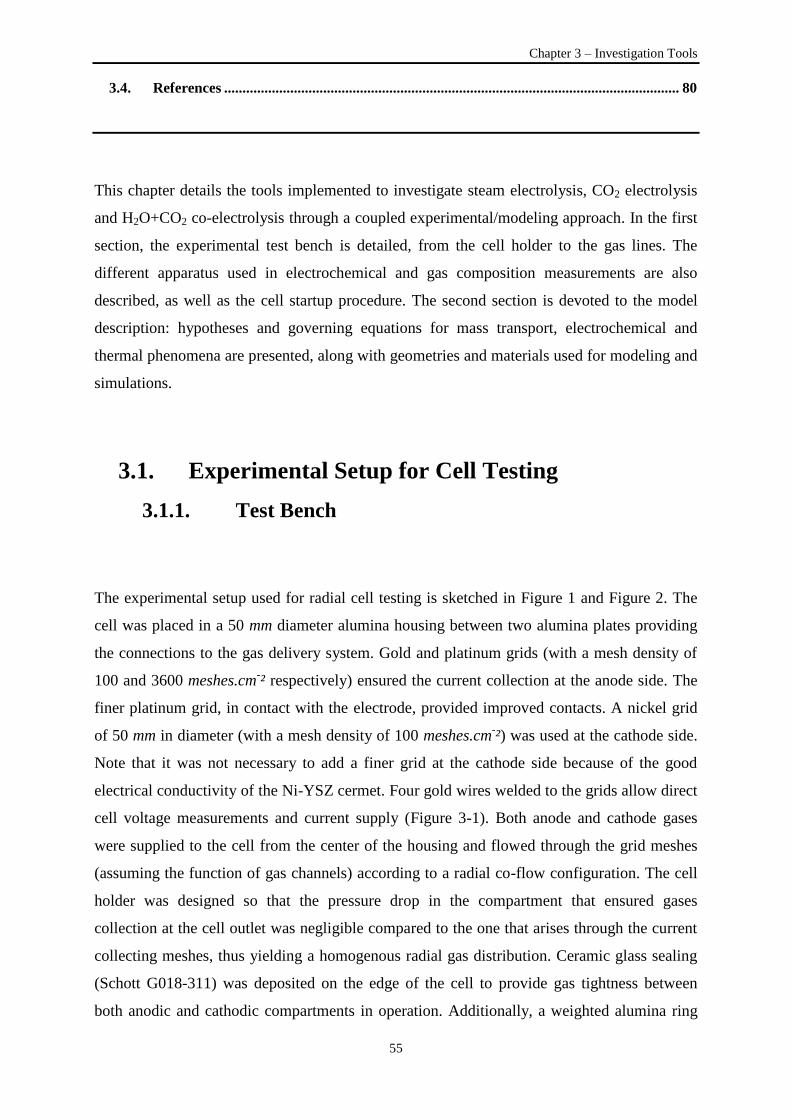
Chapter 3 – Investigation Tools
55
3.4. References ............................................................................................................................ 80
This chapter details the tools implemented to investigate steam electrolysis, CO2 electrolysis
and H2O+CO2 co-electrolysis through a coupled experimental/modeling approach. In the first
section, the experimental test bench is detailed, from the cell holder to the gas lines. The
different apparatus used in electrochemical and gas composition measurements are also
described, as well as the cell startup procedure. The second section is devoted to the model
description: hypotheses and governing equations for mass transport, electrochemical and
thermal phenomena are presented, along with geometries and materials used for modeling and
simulations.
3.1. Experimental Setup for Cell Testing
3.1.1. Test Bench
The experimental setup used for radial cell testing is sketched in Figure 1 and Figure 2. The
cell was placed in a 50 mm diameter alumina housing between two alumina plates providing
the connections to the gas delivery system. Gold and platinum grids (with a mesh density of
100 and 3600 meshes.cm-² respectively) ensured the current collection at the anode side. The
finer platinum grid, in contact with the electrode, provided improved contacts. A nickel grid
of 50 mm in diameter (with a mesh density of 100 meshes.cm-²) was used at the cathode side.
Note that it was not necessary to add a finer grid at the cathode side because of the good
electrical conductivity of the Ni-YSZ cermet. Four gold wires welded to the grids allow direct
cell voltage measurements and current supply (Figure 3-1). Both anode and cathode gases
were supplied to the cell from the center of the housing and flowed through the grid meshes
(assuming the function of gas channels) according to a radial co-flow configuration. The cell
holder was designed so that the pressure drop in the compartment that ensured gases
collection at the cell outlet was negligible compared to the one that arises through the current
collecting meshes, thus yielding a homogenous radial gas distribution. Ceramic glass sealing
(Schott G018-311) was deposited on the edge of the cell to provide gas tightness between
both anodic and cathodic compartments in operation. Additionally, a weighted alumina ring
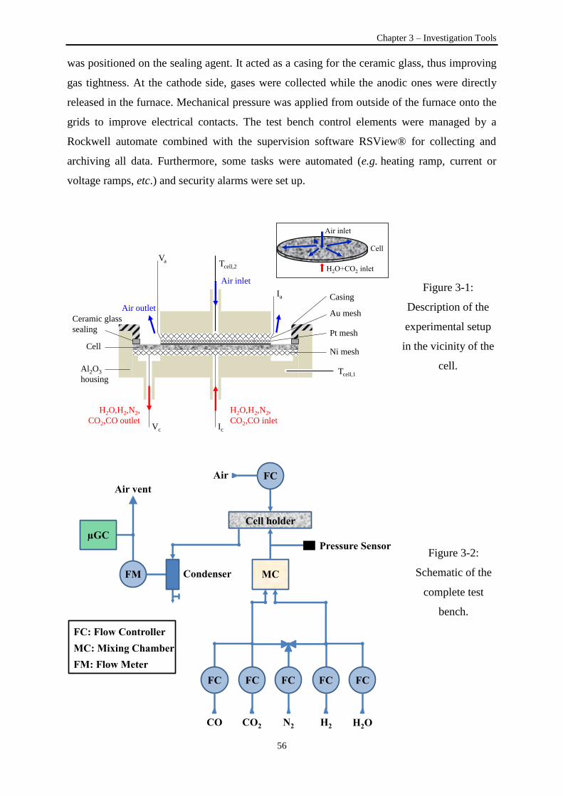
Chapter 3 – Investigation Tools
56
was positioned on the sealing agent. It acted as a casing for the ceramic glass, thus improving
gas tightness. At the cathode side, gases were collected while the anodic ones were directly
released in the furnace. Mechanical pressure was applied from outside of the furnace onto the
grids to improve electrical contacts. The test bench control elements were managed by a
Rockwell automate combined with the supervision software RSView® for collecting and
archiving all data. Furthermore, some tasks were automated (e.g. heating ramp, current or
voltage ramps, etc.) and security alarms were set up.
Figure 3-1:
Description of the
experimental setup
in the vicinity of the
cell.
Figure 3-2:
Schematic of the
complete test
bench.
Au mesh
Air inlet
H2O,H2,N2,
CO2,CO inlet
H2O,H2,N2,
CO2,CO outletVc Ic
Va
Ia
Tcell,1
Air outlet
Cell
Ceramic glass
sealing
Ni mesh
Al2O3
housing
Pt mesh
Fuel inlet
Air inlet
Cell
Casing
Tcell,2 H2O+CO2 inlet
Air inlet
Cell
Cell holder
CO CO2 N2 H2 H2O
MC: Mixing Chamber
Air
Condenser
µGC
Air vent
MC
FC FC FC FC FC
FC
FM
FC: Flow Controller
FM: Flow Meter
Pressure Sensor

Chapter 3 – Investigation Tools
57
3.1.2. Gas Lines, Steam Generation and Gases Purity
The test bench was designed to investigate SOFC, H2O electrolysis, CO2 electrolysis and co-
electrolysis operating modes. Thus, there were 6 gas lines corresponding to:
- Anode side: Air as sweeping gas
- Cathode side: H2, H2O, CO2, CO, N2
All gas lines were equipped with electrovalves and check valves and flows were controlled
with mass flow controllers (Brooks Instrument 5850S).
All gases converged toward a mixing chamber, allowing for homogeneous mixing before
reaching the cell. Due to some dead space in the test bench when operating in single H2O
electrolysis mode, nitrogen was systematically added to the inlets.
Several studies [1, 2] have shown that impurities contained in the inlet gas can cause severe
cell degradation. Thus, gas purity could be a significant factor, especially when studying cell
behavior over long periods. The following Table 3-1 summarizes the characteristics of the
different gases used. For all experiments carried out in this work, class 1 ISO 8573-
1 pressurized air was used at the anode side.
Gas Purity Supplier Impurities (vol-ppm)
Ar CO2 O2 N2 H2O H2 HC (C1-C4) CO NOx H2S
H2 3.5 Air Products <10 <10
N2 4.8 Air Products <5 <3
CO 4.5 Air Liquide <7 <1 <5 <10 <3 <1 <2
CO2 4.5 Air Products <3 <5 <5 <2 <1
Table 3-1: Available characteristics of gases used in electrolysis investigations.
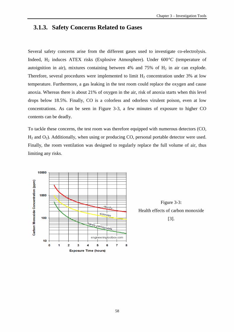
Chapter 3 – Investigation Tools
58
3.1.3. Safety Concerns Related to Gases
Several safety concerns arise from the different gases used to investigate co-electrolysis.
Indeed, H2 induces ATEX risks (Explosive Atmosphere). Under 600°C (temperature of
autoignition in air), mixtures containing between 4% and 75% of H2 in air can explode.
Therefore, several procedures were implemented to limit H2 concentration under 3% at low
temperature. Furthermore, a gas leaking in the test room could replace the oxygen and cause
anoxia. Whereas there is about 21% of oxygen in the air, risk of anoxia starts when this level
drops below 18.5%. Finally, CO is a colorless and odorless virulent poison, even at low
concentrations. As can be seen in Figure 3-3, a few minutes of exposure to higher CO
contents can be deadly.
To tackle these concerns, the test room was therefore equipped with numerous detectors (CO,
H2 and O2). Additionally, when using or producing CO, personal portable detector were used.
Finally, the room ventilation was designed to regularly replace the full volume of air, thus
limiting any risks.
Figure 3-3:
Health effects of carbon monoxide
[3].
Chapter 3 – Investigation Tools
59
3.1.4. Measuring Equipment
Most of the experimental data presented in this work are polarization curves (i-V), gas
analyses and electrochemical impedance spectroscopy measurements. This section details the
different apparatus used in this work.
3.1.4.1. Polarization curves
Electrochemical performances were studied in a galvanostatic mode using a
potentiostat/galvanostat (PGSTAT-302N Autolab), equipped with a FRA2 module and a 10 A
booster. However, when testing cells of large active areas (e.g. 9.08 cm² for a radial cell of 34
mm diameter), the current was supplied using a Xantrex XPD 33-16 DC power supply. Most
of i-V curves were recorded at a sweep rate of 10 mA.s-1
. However, in order to save time, a
sweep rate of 25 mA.s-1
was set to obtain polarization curves under high cathodic flows. Initial
experiments confirmed that increasing the sweep rate from 10 to 25 mA.s-1
had no impact in
the chosen conditions.
3.1.4.2. Gas analyses
Cell outlet compositions were determined by micro gas chromatography (µGC) using an SRA
R-3000 apparatus, equipped with a thermal conductivity detector and two separating columns.
The first column was equipped with a molecular sieve 10 m-MS5A with backflush injection
and Ar as carrier gas. It allowed the identification of H2, O2, N2, CH4 and CO. The second
column was a 8 m-Paraplot U with variable injection. Feeded with He, it detected CO2,
ethane, propane and other heavier hydrocarbons. Characteristics of carrier gases are given in
Table 3-2. It is worth noting that exhaust gas compositions were analyzed by µGC after
steam/water removal, to avoid condensation in the columns. Thus, a condenser was placed at
the cathode outlet (Figure 3-2), and the chromatograph was equipped with a water filter.
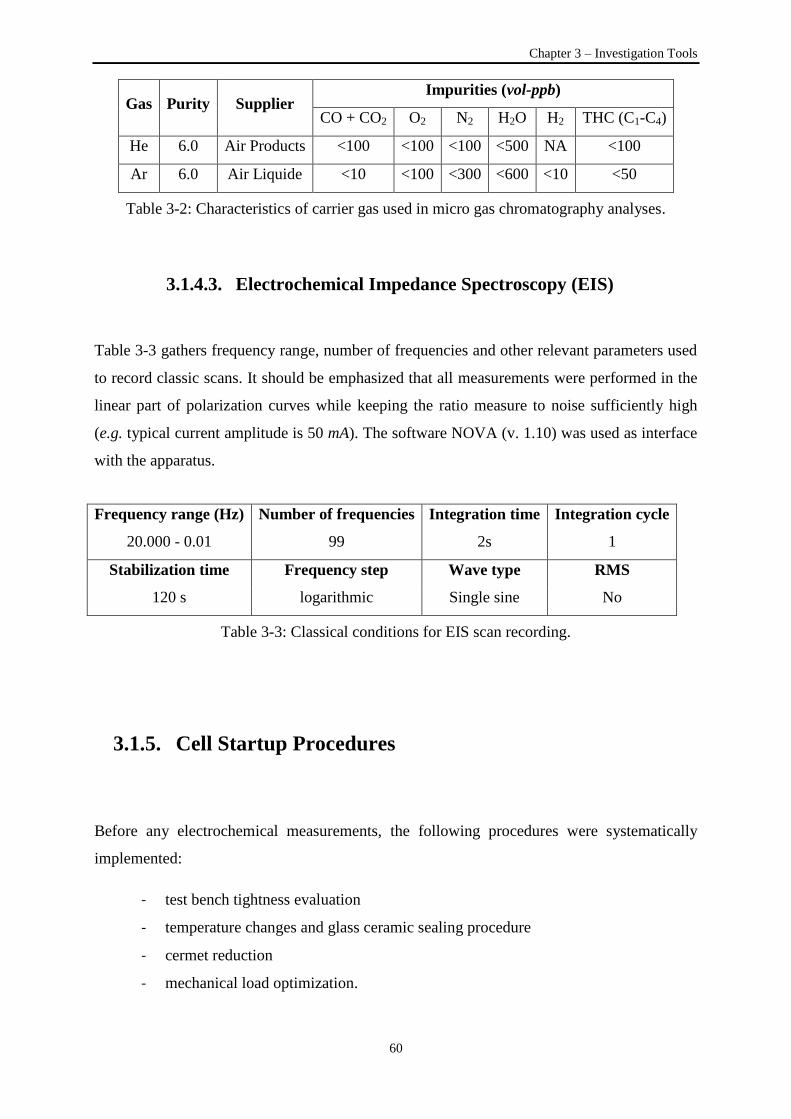
Chapter 3 – Investigation Tools
60
Gas Purity Supplier Impurities (vol-ppb)
CO + CO2 O2 N2 H2O H2 THC (C1-C4)
He 6.0 Air Products <100 <100 <100 <500 NA <100
Ar 6.0 Air Liquide <10 <100 <300 <600 <10 <50
Table 3-2: Characteristics of carrier gas used in micro gas chromatography analyses.
3.1.4.3. Electrochemical Impedance Spectroscopy (EIS)
Table 3-3 gathers frequency range, number of frequencies and other relevant parameters used
to record classic scans. It should be emphasized that all measurements were performed in the
linear part of polarization curves while keeping the ratio measure to noise sufficiently high
(e.g. typical current amplitude is 50 mA). The software NOVA (v. 1.10) was used as interface
with the apparatus.
Frequency range (Hz) Number of frequencies Integration time Integration cycle
20.000 - 0.01 99 2s 1
Stabilization time Frequency step Wave type RMS
120 s logarithmic Single sine No
Table 3-3: Classical conditions for EIS scan recording.
3.1.5. Cell Startup Procedures
Before any electrochemical measurements, the following procedures were systematically
implemented:
- test bench tightness evaluation
- temperature changes and glass ceramic sealing procedure
- cermet reduction
- mechanical load optimization.
Chapter 3 – Investigation Tools
61
3.1.5.1. Test bench tightness evaluation
The total test bench volume was initially determined using the ideal gas law, a pressure sensor
and a chronometer: by closing the outlet gas pipe just before the air vent (Figure 3-2) and
measuring the time ∆t corresponding to a pressure increase ∆P induced by a known N2 flow,
the bench volume could be assessed. Consequently, prior to each cell testing, the leakage rate
(function of the volume) was consistently measured to evaluate the tightness of the setup. The
maximum acceptable leakage was set to 1 mbar.L.min-1
at ∆P = 30 mbars, which corresponds
roughly to 1% of total flows fed to the cathode during electrochemical measurements at
∆Poperation ≈ 2 mbars.
3.1.5.2. Temperature changes and glass ceramic sealing
procedure
Once the cell was placed in the cell holder, it was heated up above 800°C, while the cathode
was fed with pure nitrogen and the anode with air. All heating and cooling rates were equal to
1°C.min-1
. After a step above 800°C, the temperature was decreased down to 800°C. This
procedure allowed the ceramic glass to act as a seal by providing gas tightness between
anodic and cathodic compartments.
3.1.5.3. Cermet reduction
Once the cell temperature was stabilized at 800°C, the nickel oxide in the cermet cathode was
reduced to metallic nickel Ni by feeding the electrode with a mixture of nitrogen and
hydrogen. Step by step (10 min long), the amount of H2 was gradually increased while
reducing the N2 flow, so that the total flow remained constant at 12 NmL.min-1
.cm-2
from pure
nitrogen to pure hydrogen. Figure 3-4 displays an example of cermet reduction by plotting the
cell OCV versus the time. Changes in inlet composition can be noticed by the sudden drops
(i.e. when the nitrogen flow is lowered) and increases in cell voltage.
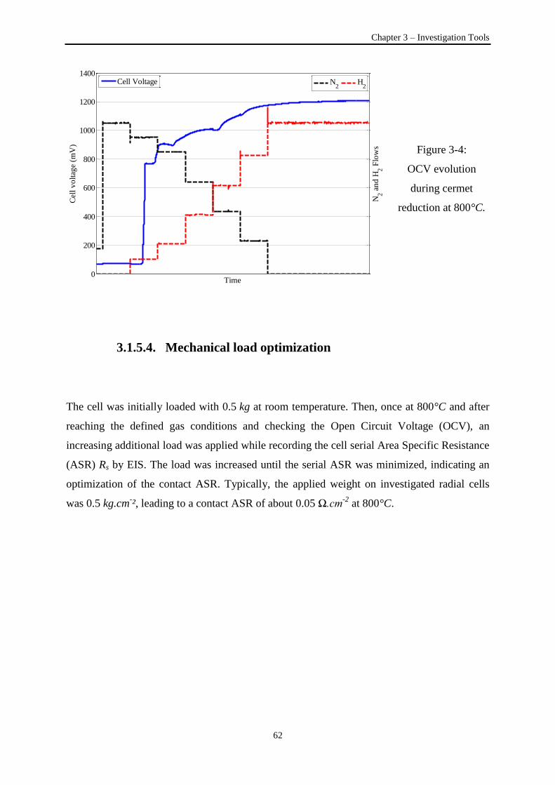
Chapter 3 – Investigation Tools
62
Figure 3-4:
OCV evolution
during cermet
reduction at 800°C.
3.1.5.4. Mechanical load optimization
The cell was initially loaded with 0.5 kg at room temperature. Then, once at 800°C and after
reaching the defined gas conditions and checking the Open Circuit Voltage (OCV), an
increasing additional load was applied while recording the cell serial Area Specific Resistance
(ASR) Rs by EIS. The load was increased until the serial ASR was minimized, indicating an
optimization of the contact ASR. Typically, the applied weight on investigated radial cells
was 0.5 kg.cm-², leading to a contact ASR of about 0.05 Ω.cm
-2 at 800°C.
0
200
400
600
800
1000
1200
1400
Time
Cel
l v
olt
age
(mV
)
Cell Voltage
N2 a
nd
H2 F
low
s
N2
H2
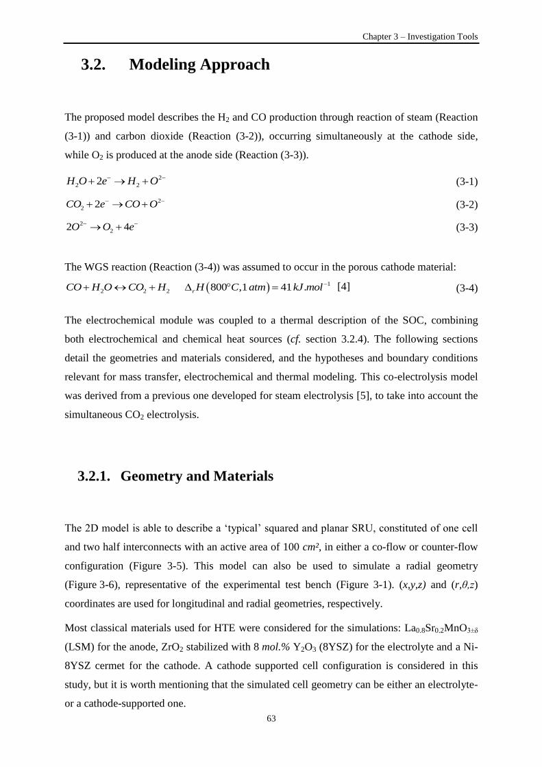
Chapter 3 – Investigation Tools
63
3.2. Modeling Approach
The proposed model describes the H2 and CO production through reaction of steam (Reaction
(3-1)) and carbon dioxide (Reaction (3-2)), occurring simultaneously at the cathode side,
while O2 is produced at the anode side (Reaction (3-3)).
2
2 22H O e H O (3-1)
2
2 2CO e CO O (3-2)
2
22 4O O e (3-3)
The WGS reaction (Reaction (3-4)) was assumed to occur in the porous cathode material:
1
2 2 2 800 ,1 41 .rCO H O CO H H C atm kJ mol [4] (3-4)
The electrochemical module was coupled to a thermal description of the SOC, combining
both electrochemical and chemical heat sources (cf. section 3.2.4). The following sections
detail the geometries and materials considered, and the hypotheses and boundary conditions
relevant for mass transfer, electrochemical and thermal modeling. This co-electrolysis model
was derived from a previous one developed for steam electrolysis [5], to take into account the
simultaneous CO2 electrolysis.
3.2.1. Geometry and Materials
The 2D model is able to describe a ‘typical’ squared and planar SRU, constituted of one cell
and two half interconnects with an active area of 100 cm², in either a co-flow or counter-flow
configuration (Figure 3-5). This model can also be used to simulate a radial geometry
(Figure 3-6), representative of the experimental test bench (Figure 3-1). (x,y,z) and (r,θ,z)
coordinates are used for longitudinal and radial geometries, respectively.
Most classical materials used for HTE were considered for the simulations: La0.8Sr0.2MnO3±δ
(LSM) for the anode, ZrO2 stabilized with 8 mol.% Y2O3 (8YSZ) for the electrolyte and a Ni-
8YSZ cermet for the cathode. A cathode supported cell configuration is considered in this
study, but it is worth mentioning that the simulated cell geometry can be either an electrolyte-
or a cathode-supported one.
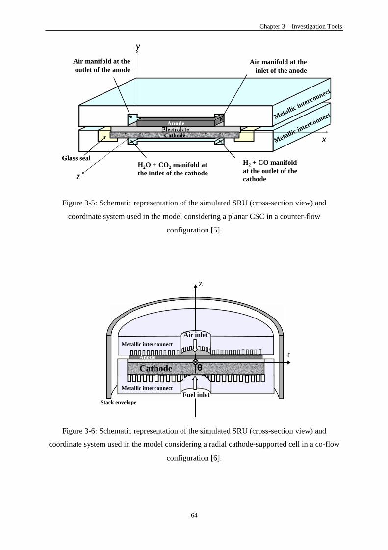
Chapter 3 – Investigation Tools
64
Figure 3-5: Schematic representation of the simulated SRU (cross-section view) and
coordinate system used in the model considering a planar CSC in a counter-flow
configuration [5].
Figure 3-6: Schematic representation of the simulated SRU (cross-section view) and
coordinate system used in the model considering a radial cathode-supported cell in a co-flow
configuration [6].
Air manifold at the
outlet of anode
Air manifold at the
inlet of anode
H2 manifold at the
outlet of cathodeSteam manifold at
the inlet of cathode
Metallic in
terconnect
Metallic in
terconnect
x
y
z
Glass seal
Air manifold at the
outlet of anode
Air manifold at the
inlet of anode
H2 manifold at the
outlet of cathodeSteam manifold at
the inlet of cathode
Metallic in
terconnect
Metallic in
terconnect
x
y
z
Glass sealH2O + CO2 manifold at
the intlet of the cathode
H2 + CO manifold
at the outlet of the
cathode
Air manifold at the
outlet of the anodeAir manifold at the
inlet of the anode
Cathode
Fuel inlet
Air inlet
Cathode
Anode
Metallic interconnect
Metallic interconnect
Stack envelope
z
r
Chapter 3 – Investigation Tools
65
3.2.2. Mass Transfer Description
The pressure drop along the gas channels was supposed to be negligible. Therefore,
atmospheric conditions were assumed for the gas-phase pressure in the SRU (PT = 1 atm).
The variation of molar fractions along the gas channels (i.e. in the x or r directions in Figure
3-5 and Figure 3-6, respectively) originates from molar fluxes through the porous electrodes
(i.e. in the y or z direction, respectively). This variation was calculated by using local mass
balances performed for each species along the channels:
(3-5)
where denotes the molar flow rate in the channels for specie i, the molar flux through
the electrode, the width of the gas channel and , a stoichiometric coefficient (equal to -1
for reactants and +1 for products).
In porous electrodes, the viscous flow, which is driven by a pressure gradient, is generally
considered negligible compared to the diffusive flow [7, 8]. Such a hypothesis is especially
accurate at the cathode side since reactions (3-1)-(3-4) are equimolar. Therefore, the mass
transport through the porous electrodes (i.e. in the direction perpendicular to the gas channel
axis) was described in the frame of the Dusty Gas Model (DGM), combining the Stephan-
Maxwell and Knudsen diffusions [9]:
(3-6)
where yi is the molar fraction of specie i and PT the total pressure (= 1 atm).
The effective Knudsen and binary diffusion coefficients, and , were determined as a
function of the electrode microstructure parameters (i.e. the mean pore radius , the tortuosity
factor and the porosity ) [10–12]. In porous media such as electrodes, the following
expressions are usually employed [13]:
and (3-7)
iii eNγ
dx
dn
in iN
eiγ
dy
dy
RT
P
D
NyNy
D
N iT
n
ij,1j
effj,i
jiij
effk,i
i ∑≠
effk,iD
effj,iD
r
j,ieff
j,i Dτ
εD k,i
effk,i D
τ
εD
Chapter 3 – Investigation Tools
66
The Knudsen diffusion coefficient can be assessed according to the kinetic theory of gases:
(3-8)
where denotes the molecular weight for the gas i.
The binary diffusion coefficients have been expressed as follows [12]:
with (3-9)
where corresponds to the Füller diffusion volume of specie i.
At the anode side, a binary mixture of oxygen and nitrogen was considered as the electrode
inlet. Using the method presented in [5], an analytical solution of the DGM (Equation (3-6))
can be found, provided that the N2 flux is nil inside the electrode, and that the O2 flux is
imposed by the local current density i(x) according the Faraday law:
2 4O
iN
F (3-10)
The oxygen molar fraction at the anode/electrolyte interface can be then expressed as a
function of the electrode thickness a, the molar fraction into the anodic gas channel and
the gas constant R:
2 2 2 2 2 2 2
2 2
2 2 2 2 2
, , , , ,
, , , ,
exp4
eff eff eff eff eff
O k O N O k O N O kint canal
O O aeff eff eff eff
O k O k T O k O N
D D D D DiRTy y
D D P F D D
(3-11)
At the cathode side, the total current is generated by electrochemical reduction of H2O and
CO2 (Reactions (3-1) and (3-2)). Therefore, the local current can be split into two
contributions and related to H2O and CO2 reduction reactions. At the
electrode/electrolyte interface, the molar fluxes can be then expressed as a function of these
two components:
with and (y=0) (3-12)
Moreover, the occurrence of the WGS reaction (Reaction (4)) within the cathode can produce
or consume species involved in electrochemical reactions. These source terms modify the
fluxes according to the following mass balances:
ik,i
Mπ
RT8
3
2rD
iM
23/1j
3/1i
2/1j,iT
75.1
j,i)VV(MP
T00143,0D
jij,i
M
1
M
1/2M
iV
intO2
y
canalO2
y
2HI COI
2HCO III dSF2
INN CO
COCO2
dSF2
INN 2
22
H
HOH
Chapter 3 – Investigation Tools
67
, ,i idN x y r x y dy with i = H2, H2O, CO et CO2. (3-13)
where ri is the molar rate of formation per unit volume of the porous medium written for each
gas species i.
This term is linked to the WGS reaction rate vWGS which is assumed to occur in the void
fraction of the cermet:
and (3-14)
where is the cermet porosity.
The WGS reaction kinetic rate can be expressed as follows:
(3-15)
where k+ and k- are the kinetic constants of forward and backward reactions.
The kinetic constants are calculated as a function of the WGS reaction activation energy
WGS
aE :
0 0exp expWGS WGS
a aE EkTk f k
RT RT
and ek k K (3-16)
where Ke is the thermodynamic equilibrium constant for the WGS reaction.
Numerical values used to assess the WGS kinetic can be found in Table 3-4.
eK
978 K 1018 K 1078 K 1118 K 1178 K
1.58 1.34 1.07 0.93 0.78
WGS
aE = 103800 J.mol-1
0k = 1.88 ×10⁸ mol.s
-1.bar
-2.m
-3
Table 3-4 : Kinetic values for WGS reaction kinetics [14, 15].
In this model, the reactions of carbon deposition and methane production were not
considered. Indeed, thermodynamic predictions [16] and experimental reports [17]
demonstrated that methane production is negligible at atmospheric pressure and high
temperature. Similarly, in a high temperature co-electrolyzer operating at atmospheric
pressure, thermodynamic calculations [18] have shown that carbon deposition is not favored
in presence of H2O and/or CO2. However, if CO becomes largely preponderant at high CO2
and H2O conversion rates, carbon formation becomes likely. In such peculiar operating
conditions, the carbon deposit could yield deactivation of active sites and could be a limiting
factor and a source of degradation.
WGSCOH vεrr22
WGSCOOH vεrr22
222 HCOOHCOWGS yykyykv
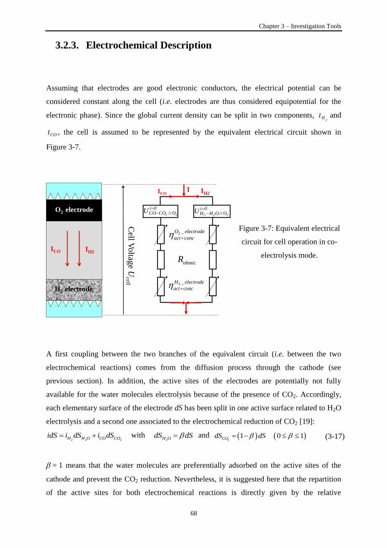
Chapter 3 – Investigation Tools
68
3.2.3. Electrochemical Description
Assuming that electrodes are good electronic conductors, the electrical potential can be
considered constant along the cell (i.e. electrodes are thus considered equipotential for the
electronic phase). Since the global current density can be split in two components, and
, the cell is assumed to be represented by the equivalent electrical circuit shown in
Figure 3-7.
Figure 3-7: Equivalent electrical
circuit for cell operation in co-
electrolysis mode.
A first coupling between the two branches of the equivalent circuit (i.e. between the two
electrochemical reactions) comes from the diffusion process through the cathode (see
previous section). In addition, the active sites of the electrodes are potentially not fully
available for the water molecules electrolysis because of the presence of CO2. Accordingly,
each elementary surface of the electrode dS has been split in one active surface related to H2O
electrolysis and a second one associated to the electrochemical reduction of CO2 [19]:
2 2 2H H O CO COidS i dS i dS with 2H OdS dS and
21COdS dS 0 1 (3-17)
= 1 means that the water molecules are preferentially adsorbed on the active sites of the
cathode and prevent the CO2 reduction. Nevertheless, it is suggested here that the repartition
of the active sites for both electrochemical reactions is directly given by the relative
2HI
COI
IH2
I
Cell
Vo
ltage U
cell
IH2
O2 electrode
H2 electrode
ICO
0iO//OHH 222
U
2 _O electrode
act conc
ohmicR
2 _H electrode
act conc
0iO//COCO 22
U
ICO
Chapter 3 – Investigation Tools
69
percentage of H2O and CO2 at the cathode/electrolyte interface. In this view, the surface ratio
β can be expressed as follows [19]:
(3-18)
β represents, at the macroscopic scale, the competition between H2O and CO2 electrolyses
over the same active sites. In other words, it translates adsorption/desorption and charge
transfer phenomena competition, and more specifically, the readiness of steam electrolysis
compared to CO2 electrolysis.
Considering the equivalent electrical circuit in Figure 3-7, both current densities must be
determined from Equations (3-19) and (3-20), obtained from a decomposition of the general
Butler-Volmer expression. These equations are written assuming that the local current
densities are negative in the electrolysis mode. For each slice of cell laying between x and
x+dx (Figure 3-5), the cell voltage is expressed as functions of the equilibrium potential, the
ohmic losses and the different overpotentials related to the H2-H2O//O2 and CO-CO2//O2
electrochemical systems:
2 2 2
2 2 2 2 2 2 2 2 2 2 2 2 2
/ /
0 , / / , / / , / / , / /
H H O O anode cathode anode cathode
cell i ohm H act H H O O act H H O O conc H H O O conc H H O OU U R i
(for ) (3-19)
2 2
2 2 2 2 2 2 2 2
/ /
0 , / / , / / , / / , / /
CO CO O anode cathode anode cathode
cell i ohm CO act CO CO O act CO CO O conc CO CO O conc CO CO OU U R i
(for ) (3-20)
where Ui=0 is the Open Circuit Voltage (OCV) computed from the Nernst equation:
(3-21)
(3-22)
where are the molar fractions taken at the cathode/electrolyte interface and
denotes the oxygen molar fraction calculated at the anode/electrolyte interface at i=0.
It is worth emphasizing that the OCV evolves along the cell length because of the WGS
reaction which modifies the partial pressures even at i=0. For both electrochemical systems,
intOH
intCO
intOH 222
yyyβ
OH2dS
2COdS
0iint_
OH
0iint_
O
0iint_
H0O//OHH
O//OHH0i
2
22
222
222
y
yyln
F2
RT)T(U)x(U
0iint_
CO
0iint_
O
0iint_CO0
O//COCOO//COCO
0i
2
2
22
22
y
yyln
F2
RT)T(U)x(U
0iint_
CO,CO,OH,Hi 222y
0iint_
Oi 2y
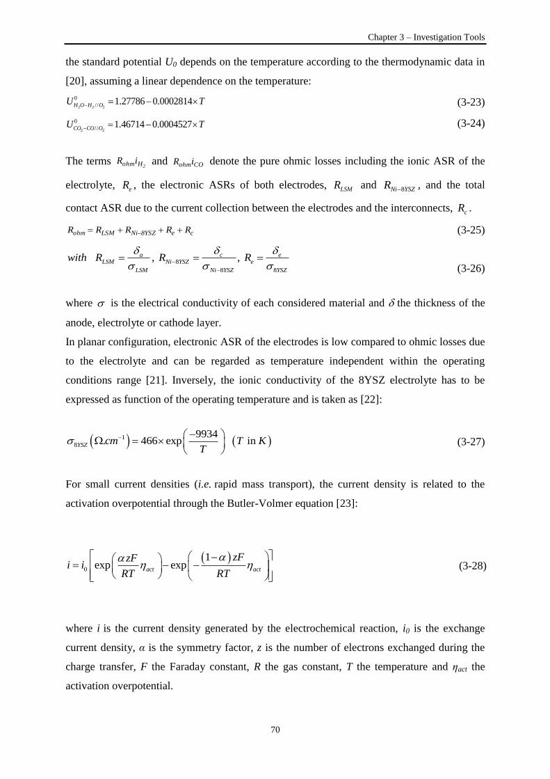
Chapter 3 – Investigation Tools
70
the standard potential U0 depends on the temperature according to the thermodynamic data in
[20], assuming a linear dependence on the temperature:
2 2 2
0
// 1.27786 0.0002814H O H OU T (3-23)
2 2
0
// 1.46714 0.0004527CO CO OU T (3-24)
The terms and denote the pure ohmic losses including the ionic ASR of the
electrolyte, eR , the electronic ASRs of both electrodes, LSMR and 8Ni YSZR , and the total
contact ASR due to the current collection between the electrodes and the interconnects, cR .
8
8 8
, , a c eLSM Ni YSZ e
LSM Ni YSZ YSZ
with R R R
(3-25)
(3-26)
where is the electrical conductivity of each considered material and the thickness of the
anode, electrolyte or cathode layer.
In planar configuration, electronic ASR of the electrodes is low compared to ohmic losses due
to the electrolyte and can be regarded as temperature independent within the operating
conditions range [21]. Inversely, the ionic conductivity of the 8YSZ electrolyte has to be
expressed as function of the operating temperature and is taken as [22]:
1
8
9934. 466 exp in YSZ cm T K
T
(3-27)
For small current densities (i.e. rapid mass transport), the current density is related to the
activation overpotential through the Butler-Volmer equation [23]:
0
1exp expact act
zFzFi i
RT RT
(3-28)
where i is the current density generated by the electrochemical reaction, i0 is the exchange
current density, α is the symmetry factor, z is the number of electrons exchanged during the
charge transfer, F the Faraday constant, R the gas constant, T the temperature and ηact the
activation overpotential.
2HohmiRCOohmiR
ceYSZ8NiLSMohm RRRRR
Chapter 3 – Investigation Tools
71
For a co-electrolysis mode, assuming that the symmetry factor α is equal to 0.5, the activation
overpotentials are expressed as follows:
2 2
2 2 2 2 2 2 2 2
1 1
, / / , / /
0, 0,
sinh sinh2 2
H Hanode cathode
act H H O O act H H O O H H O
anode cathode
i iRT
F i i
(3-29)
2 2 2 2 2
1 1
, / / , / /
0, 0,
sinh sinh2 2
CO COanode cathode
act CO CO O act CO CO O CO CO
anode cathode
i iRT
F i i
(3-30)
The exchange current density i0 represents the capacity of the electrode to proceed with the
electrochemical reaction. It is a measure of the forward and backward rate constants at the
equilibrium. The higher the exchange current density, the higher is the electrochemical
reaction rate for a given electrode overpotential. The activation overpotential thus represents
the voltage loss induced by the electrochemical reactions.
It should be noted here that without introducing the phenomenological ‘surface ratio’
parameter β (Equation (3-18)), the specific calculation of both activation overpotentials would
lead to an overestimation of the available electroactive area by a factor 2. Indeed, solving
Equations (3-29) and (3-30) would be equivalent to assuming that all active sites are
simultaneously available for the reduction of both steam and CO2.
The concentration overpotentials can arise because the gas composition in the vicinity of the
active sites is different from the initial composition at OCV. This can be related to insufficient
gas diffusion through the electrodes or insufficient gas flow rate introduced at the anode or
cathode inlet. The concentration overpotentials can be expressed from the Nernst equation
according to:
(3-31)
(3-32)
(3-33)
0iint_
OH
0iint_
H
0iint_
OH
0iint_
HcathodeO//OHH,conc
22
22
222yy
yyln
F2
RTη
0iint_
CO
0iint_CO
0iint_
CO
0iint_COcathode
O//2COCO,conc
2
2
2yy
yyln
F2
RTη
0iint_
O
0iint_
OanodeO//COCO,conc
anodeO//OHH,conc
2
2
22222y
yln
F4
RTηη
Chapter 3 – Investigation Tools
72
In the proposed model, the molar fractions are taken at the anode or cathode active sites
(i.e. the Triple Phase Boundary lengths), which were reduced to the anode/electrolyte or
cathode/electrolyte interfaces. It is worth noting that this assumption is well verified for
sufficiently thick electrodes. Indeed, numerous studies [7, 24, 25] showed that the reaction
zone spreads on a limited region from the electrolyte/electrode interface within the electrode
(~10-20 µm). In this work, the improvement of the electrode efficiency due to the extent of
the electrochemical reactions is taken into account in the ‘apparent’ exchange current
densities including the ‘global’ electrochemical process into the active layers [26].
3.2.4. Thermal Description
The thermal model used for co-electrolysis simulations has been adapted from a previous one
developed for steam electrolysis and SOFC modes detailed in [5, 6]. The main assumptions
are summarized in this section. It is worth noting that the evolutions of all variables with the
geometry are taken into account (e.g. temperatures, partial pressures, heat transfer
coefficients, surface element variation in the specific case of radial cell geometries… as
functions of (x,y) or (z,θ)). However, for the sake of clarity, some of the dependences are not
expressed in following equations. Additional details and numerical input data concerning this
thermal description can be found in Chapter 5 and in references [5, 6].
Adiabatic conditions were assumed for the surfaces connecting two adjacent SRUs (i.e. the
bottom and top free surfaces of SRU as shown on Figure 3-8). This assumption is well
verified only for the SRUs located in the central region of the stack where heat flux in the
stacking direction can be neglected. The temperatures of gases introduced into the SRU were
chosen equal to Tinsulating. The temperature of the insulating envelope surrounding the stack
was supposed to be controlled by Tinsulating.
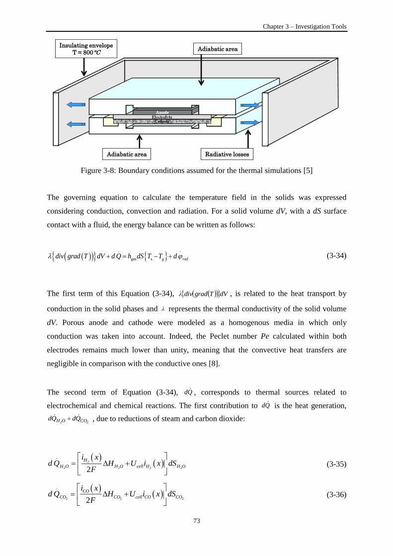
Chapter 3 – Investigation Tools
73
Figure 3-8: Boundary conditions assumed for the thermal simulations [5]
The governing equation to calculate the temperature field in the solids was expressed
considering conduction, convection and radiation. For a solid volume dV, with a dS surface
contact with a fluid, the energy balance can be written as follows:
. .
radgas s gdiv grad T dV d Q h dS T T d (3-34)
The first term of this Equation (3-34), , is related to the heat transport by
conduction in the solid phases and represents the thermal conductivity of the solid volume
dV. Porous anode and cathode were modeled as a homogenous media in which only
conduction was taken into account. Indeed, the Peclet number Pe calculated within both
electrodes remains much lower than unity, meaning that the convective heat transfers are
negligible in comparison with the conductive ones [8].
The second term of Equation (3-34), , corresponds to thermal sources related to
electrochemical and chemical reactions. The first contribution to is the heat generation,
, due to reductions of steam and carbon dioxide:
2
2 2 22
.
2
H
H O cell H H OH O
i xd Q H U i x dS
F
(3-35)
2 22
.
2
CO
CO cell CO COCO
i xd Q H U i x dS
F
(3-36)
Radiative losses
Adiabatic areaInsulating envelope
T = 800°C
Adiabatic area
dVTgraddivλ
λ
Qd
Qd
22 COOH QdQd
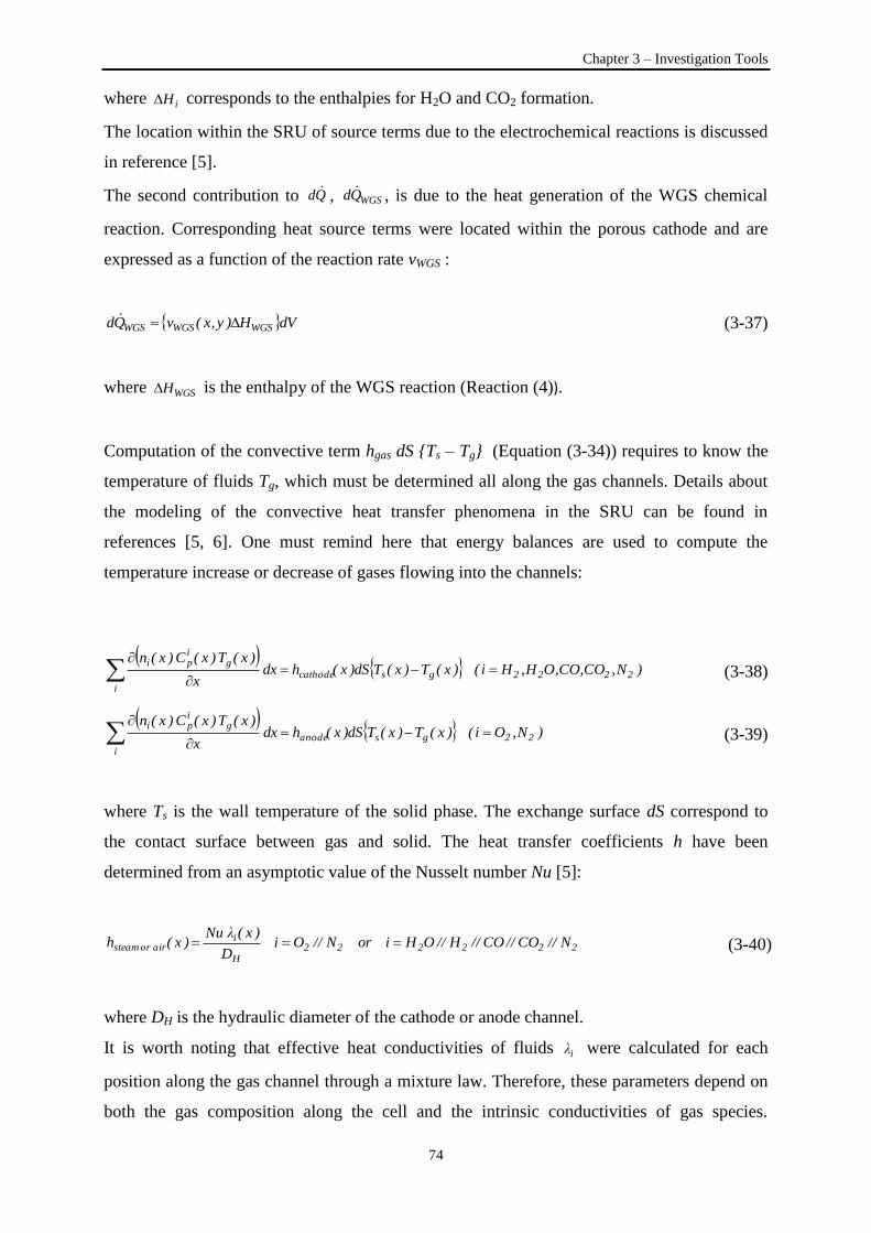
Chapter 3 – Investigation Tools
74
where corresponds to the enthalpies for H2O and CO2 formation.
The location within the SRU of source terms due to the electrochemical reactions is discussed
in reference [5].
The second contribution to , , is due to the heat generation of the WGS chemical
reaction. Corresponding heat source terms were located within the porous cathode and are
expressed as a function of the reaction rate vWGS :
(3-37)
where is the enthalpy of the WGS reaction (Reaction (4)).
Computation of the convective term hgas dS Ts – Tg (Equation (3-34)) requires to know the
temperature of fluids Tg, which must be determined all along the gas channels. Details about
the modeling of the convective heat transfer phenomena in the SRU can be found in
references [5, 6]. One must remind here that energy balances are used to compute the
temperature increase or decrease of gases flowing into the channels:
(3-38)
(3-39)
where Ts is the wall temperature of the solid phase. The exchange surface dS correspond to
the contact surface between gas and solid. The heat transfer coefficients h have been
determined from an asymptotic value of the Nusselt number Nu [5]:
(3-40)
where DH is the hydraulic diameter of the cathode or anode channel.
It is worth noting that effective heat conductivities of fluids were calculated for each
position along the gas channel through a mixture law. Therefore, these parameters depend on
both the gas composition along the cell and the intrinsic conductivities of gas species.
iH
Qd WGSQd
dVH)y,x(vQd WGSWGSWGS
WGSH
)N,CO,CO,OH,Hi()x(T)x(TdS)x(hdx
x
)x(T)x(C)x(n2222gscathode
i
gipi
)N,Oi()x(T)x(TdS)x(hdx
x
)x(T)x(C)x(n22gsanode
i
gipi
222222H
iairorsteam N//CO//CO//H//OHiorN//Oi
D
)x(λNu)x(h
iλ
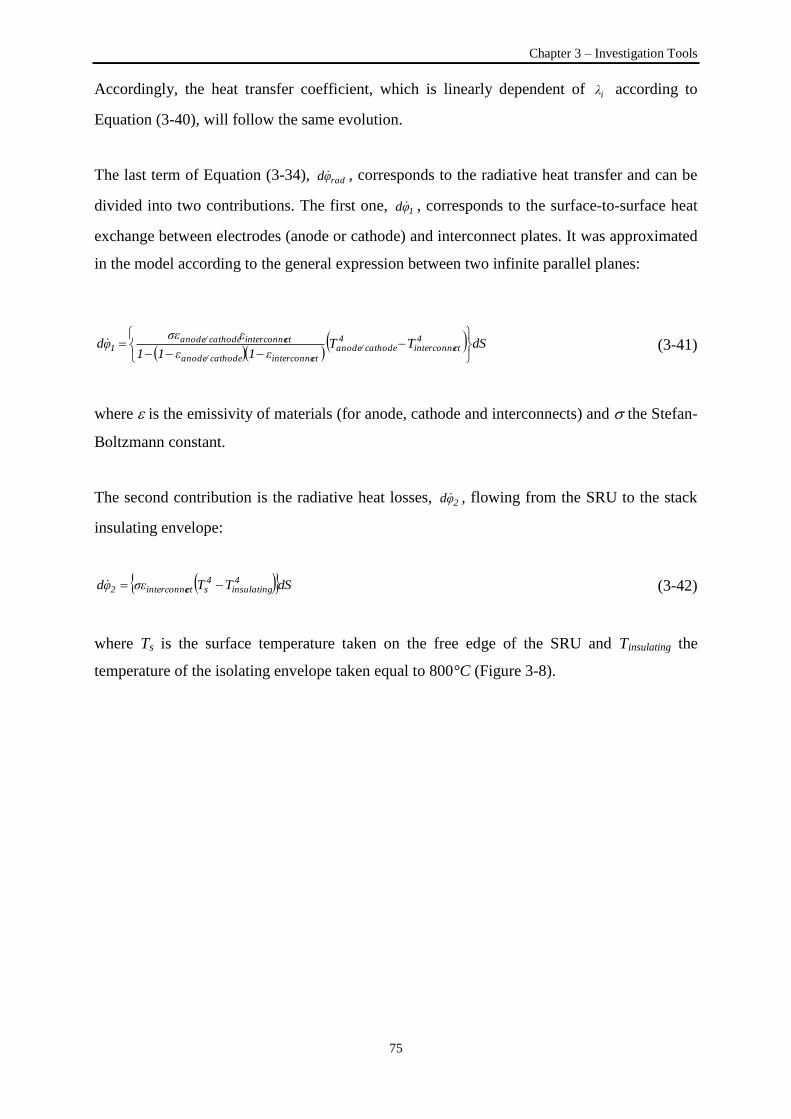
Chapter 3 – Investigation Tools
75
Accordingly, the heat transfer coefficient, which is linearly dependent of according to
Equation (3-40), will follow the same evolution.
The last term of Equation (3-34), , corresponds to the radiative heat transfer and can be
divided into two contributions. The first one, , corresponds to the surface-to-surface heat
exchange between electrodes (anode or cathode) and interconnect plates. It was approximated
in the model according to the general expression between two infinite parallel planes:
(3-41)
where is the emissivity of materials (for anode, cathode and interconnects) and the Stefan-
Boltzmann constant.
The second contribution is the radiative heat losses, , flowing from the SRU to the stack
insulating envelope:
(3-42)
where Ts is the surface temperature taken on the free edge of the SRU and Tinsulating the
temperature of the isolating envelope taken equal to 800°C (Figure 3-8).
iλ
radφd
1φd
dSTT
ε1ε11
εσεφd 4
ctinterconne4
cathode/anodectinterconnecathode/anode
ctinterconnecathode/anode1
2φd
dSTTσεφd 4insulating
4sctinterconne2

Chapter 3 – Investigation Tools
76
3.2.5. Numerical Architecture
Mass transfer and electrochemical descriptions were implemented using the commercial
software Matlab®. Thermal calculations were solved within the frame of the finite elements
code Cast3M. The computational procedures are summarized in the flowcharts given in
Figures 3-9 and 3-10.
Within the electrochemical module, the cell is divided into a mesh of elementary slices. Local
mass balances (Equation (3-5)) allow calculating gas flow in the channels from one
elementary slice to the next one. For each slice of cell, both local electrochemical currents are
determined into an iterative scheme so that Equations (3-19) and (3-20) are simultaneously
verified. These calculations, along with β (Equations (3-17) and (3-18)), encompass the
determinations of local overpotentials associated to mass transfer through the porous
electrodes. It can be mentioned that the set of equations describing diffusion and WGS
reaction within the cathode are numerically solved by a Runge-Kutta method associated with
a shooting method. For each slice of cell, the numerical solution is obtained through two main
loops running until both H2O and CO2 electrochemical currents (and the resulting diffusion
process, molar fractions distribution and β) are stable. An external loop is added all along the
cell length to ensure the convergence of the output data in a counter-flow configuration.
Once the electrochemical calculations are completed, the repartition of gas composition,
fluxes and thermal sources are used as input data for the thermal module. Heat transfer by
conduction and radiation are calculated according to a finite element analysis which has been
coupled with a finite difference method to solve the thermal convection along the gas channel.
The new temperature field throughout the SRU 2D geometry is subsequently introduced in
the electrochemical module. A global iterative loop between both modules is run until the
stability of model outputs is reached.
Chapter 3 – Investigation Tools
77
Figure 3-9:
Isothermal model summary and architecture.
Figure 3-10:
Complete model summary and architecture.
3.2.6. Numerical Reliability
As detailed in previous sections, the model is constituted by several entangled loops. They run
until a preset condition is satisfied (i.e. the computed error is smaller than the maximum
acceptable error). These acceptable errors are detailed in this section in order to explicit the
numerical accuracy.
3.2.6.1. Loops on each current density
Both current densities were determined so that the computed cell voltage equals the set
voltage (Equations (3-19) and (3-20)) within a margin of relative error of 5×10⁻⁵
V.V-1
. This
amounts to a maximum error of 0.1 mV at 1.5 V.
Iterative
calculation
...
Start of calculation: T = 800 C
Mesh element
k-1
Mesh element
k+1
Element k
Electrochemical module in Matlab®
Solution : T = 800 C
Mass balance
Mass balance
2 H COi and i
2 2 2
6
/ / / 10H O H O cell cellU U U
2 2
6
/ / / 10CO CO O cell cellU U U
diffusion
overpotentials
...until
Ω
Iterative
calculation
...
Initial field of temperature
Mesh element
k-1
Mesh element
k+1
Element k
Electrochemical module in Matlab®
Distribution of thermal sources
and evolutions of gas compositions
Calculation of a new 2D field of temperatureConvective, diffusive and radiative fluxes computed by
finite elements method coupled with finite difference method
Thermal module in Cast3M
Comparison with previous range of temperature
Stable solution Unstable solution
Mass balance
Mass balance
2 H COi and i
2 2 2
6
/ / / 10H O H O cell cellU U U
2 2
6
/ / / 10CO CO O cell cellU U U
diffusion
overpotentials
...until
Chapter 3 – Investigation Tools
78
3.2.6.2. Loop on global current density stability
Once both current densities were determined, a new value for the surface ratio β was
computed from the resulting molar fractions. Even small variations of β can lead to significant
changes for 2Hi and
COi . Hence, before performing calculations on the adjacent mesh, the
relative change between two consecutive global current densities determined iteratively has to
be lower than 1% (i.e. <0.02 A.cm-2
if the absolute local current density is 2 A.cm-2
).
3.2.6.3. Loop on counter flow
When simulating a counter-flow configuration, the outlet air flow is assumed. Calculations
follow the cathodic flow, thus the computed oxygen content in the anodic flow decreases
element after element through local mass balances resulting from local electrochemical
production. When reaching the last element of the cell length (i.e. cathodic outlet and anodic
inlet), the resulting oxygen flow is compared to the known inlet one. The loop is exited when
this relative error is lower than 2%.
The maximum acceptable error was adjusted from calculations done with the analytical steam
reduction model. Indeed, most of the calculation time can be linked to the numerical solving
of the DGM, which is only done in co-electrolysis simulations. A 2% relative error results in
an acceptable number of iterations and has a limited influence on the resulting global current
(i.e. the difference between the global current densities obtained within a 10-6
and a 2%
relative error is lower than 0.01 A.cm-2
).
3.2.7. Model Positioning in International Literature
Recent efforts in co-electrolysis investigations have led to the development of multiple
electrochemical models (cf. 2.3) aiming at predicting both the performances and the outlet gas
compositions of an operating cell. Due to the fast WGS reaction kinetics, the vast majority of
these models assume that steam is the sole electrochemically active specie, whereas CO is
produced through the reverse WGS reaction. Conversely, M. Ni et al. [20] have proposed a
Chapter 3 – Investigation Tools
79
model taking into the CO2 reduction as well as the chemical reaction. However, to the best of
my knowledge, no models prior to this work have described the macroscopic co-electrolysis
mechanism through a splitting approach (cf. Equation (3-17)).
As already mentioned, the model described in this chapter is based on previous ones
developed to simulate SRUs or stacks operated first in SOFC mode [6], then in HTE mode
[5]. Nevertheless, the proposed model differs from these predecessors mainly by the
description of the diffusion, which now considers up to 5 species, and by two hereby
introduced and strong hypotheses that are an approach based on a parallel equivalent electrical
circuit and a coupling of the two branches through a surface ratio parameter.
3.3. Conclusion
The experimental and modeling tools detailed in this chapter have been used to investigate the
cell responses in steam electrolysis, carbon dioxide electrolysis and co-electrolysis modes.
Single electrolysis measurements were devoted to determining the unknown parameters
before simulating co-electrolysis operations. Throughout this work, no parameters have been
adjusted using co-electrolysis data. Experimental results and corresponding simulations are
presented in the following chapters, intended for model validation and simulations results.
Chapter 3 – Investigation Tools
80
3.4. References
1. S. D. Ebbesen, C. Graves, and M. Mogensen, Production of Synthetic Fuels by Co-Electrolysis of
Steam and Carbon Dioxide, Int. J. Green Energy 6, 646 (2009).
2. S. D. Ebbesen, C. Graves, A. Hauch, S. H. Jensen, and M. Mogensen, Poisoning of Solid Oxide
Electrolysis Cells by Impurities, J. Electrochem. Soc. 157, B1419 (2010).
3. http://www.engineeringtoolbox.com/carbon-monoxide-d_893.html
4. J. Xu and G. F. Froment, Methane steam reforming, methanation and water-gas shift: I. Intrinsic
kinetics, AIChE J. 35, 88 (1989).
5. J. Laurencin, D. Kane, G. Delette, J. Deseure, and F. Lefebvre-Joud, Modelling of solid oxide
steam electrolyser: Impact of the operating conditions on hydrogen production, J. Power Sources
196, 2080 (2011).
6. J. Laurencin, F. Lefebvre-Joud, and G. Delette, Impact of cell design and operating conditions on
the performances of SOFC fuelled with methane, J. Power Sources 177, 355 (2008).
7. J.-W. Kim, Polarization Effects in Intermediate Temperature, Anode-Supported Solid Oxide Fuel
Cells, J. Electrochem. Soc. 146, 69 (1999).
8. T. Ackmann, L. G. J. de Haart, W. Lehnert, and D. Stolten, Modeling of Mass and Heat Transport
in Planar Substrate Type SOFCs, J. Electrochem. Soc. 150, A783 (2003).
9. R. Suwanwarangkul, E. Croiset, M. W. Fowler, P. L. Douglas, E. Entchev, and M. A. Douglas,
Performance comparison of Fick’s, dusty-gas and Stefan–Maxwell models to predict the
concentration overpotential of a SOFC anode, J. Power Sources 122, 9 (2003).
10. Y. Shi, N. Cai, and C. Li, Numerical modeling of an anode-supported SOFC button cell
considering anodic surface diffusion, J. Power Sources 164, 639 (2007).
11. L. Andreassi, G. Rubeo, S. Ubertini, P. Lunghi, and R. Bove, Experimental and numerical
analysis of a radial flow solid oxide fuel cell, Int. J. Hydrog. Energy 32, 4559 (2007).
12. B. Todd and J. B. Young, Thermodynamic and transport properties of gases for use in solid oxide
fuel cell modelling, J. Power Sources 110, 186 (2002).
13. T. Boëdec, M. Reytier, D. Lhachemi, D. Tschumperlé, P. Louat, S. Di Iorio, P. Baurens, and G.
Delette, A New Stack to Validate Technical Solutions and Numerical Simulations, Fuel Cells 12,
239 (2012).
14. W. Lehnert, J. Meusinger, and F. Thom, Modelling of gas transport phenomena in SOFC anodes,
J. Power Sources 87, 57 (2000).
15. B. Morel, J. Laurencin, Y. Bultel, and F. Lefebvre-Joud, Anode-Supported SOFC Model Centered
on the Direct Internal Reforming, J. Electrochem. Soc. 152, A1382 (2005).
16. X. Sun, M. Chen, S. H. Jensen, S. D. Ebbesen, C. Graves, and M. Mogensen, Thermodynamic
analysis of synthetic hydrocarbon fuel production in pressurized solid oxide electrolysis cells, Int.
J. Hydrog. Energy 37, 17101 (2012).
17. W. Li, H. Wang, Y. Shi, and N. Cai, Performance and methane production characteristics of
H2O–CO2 co-electrolysis in solid oxide electrolysis cells, Int. J. Hydrog. Energy 38, 11104
(2013).
Chapter 3 – Investigation Tools
81
18. W. Y. Lee, J. Hanna, and A. F. Ghoniem, On the Predictions of Carbon Deposition on the Nickel
Anode of a SOFC and Its Impact on Open-Circuit Conditions, J. Electrochem. Soc. 160, F94
(2012).
19. J. Aicart, J. Laurencin, M. Petitjean, and L. Dessemond, Experimental Validation of Co-
Electrolysis Modeling, Proc. 2013 FDFC Congr. (2013).
20. M. Ni, An electrochemical model for syngas production by co-electrolysis of H2O and CO2, J.
Power Sources 202, 209 (2012).
21. C. Stiller, B. Thorud, S. Seljebø, Ø. Mathisen, H. Karoliussen, and O. Bolland, Finite-volume
modeling and hybrid-cycle performance of planar and tubular solid oxide fuel cells, J. Power
Sources 141, 227 (2005).
22. A. Weber and E. Ivers-Tiffée, Materials and concepts for solid oxide fuel cells (SOFCs) in
stationary and mobile applications, Eighth Ulm. Electrochem. Tage 127, 273 (2004).
23. W. G. Bessler, J. Warnatz, and D. G. Goodwin, The influence of equilibrium potential on the
hydrogen oxidation kinetics of SOFC anodes, Solid State Ion. 177, 3371 (2007).
24. S. B. Adler, Mechanism and kinetics of oxygen reduction on porous La1−xSrxCoO3−δ electrodes,
Solid State Ion. 111, 125 (1998).
25. S. Primdahl and M. Mogensen, Oxidation of hydrogen on Ni/yttria-stabilized zirconia cermet
anodes, J. Electrochem. Soc. 144, 3409 (1997).
26. F. Usseglio-Viretta, J. Laurencin, G. Delette, J. Villanova, P. Cloetens, and D. Leguillon,
Quantitative microstructure characterization of a Ni–YSZ bi-layer coupled with simulated
electrode polarisation, J. Power Sources 256, 394 (2014).

Chapter 4 – Model Validation
82
Chapter 4
Model Validation

Chapter 4 – Model Validation
83
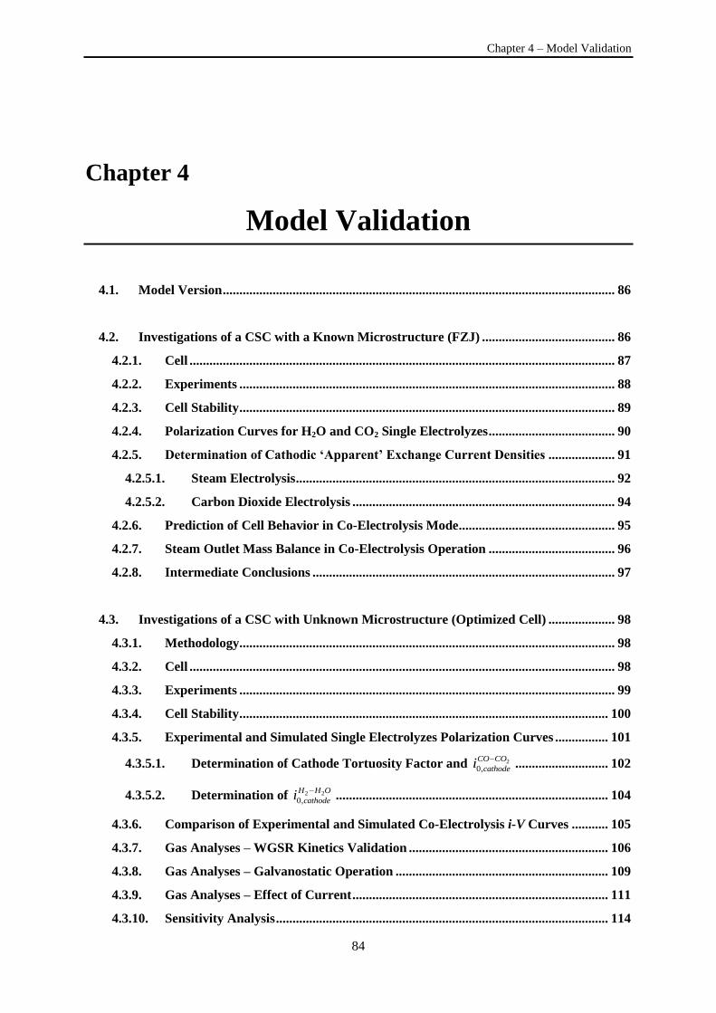
Chapter 4 – Model Validation
84
Chapter 4
Model Validation
4.1. Model Version ...................................................................................................................... 86
4.2. Investigations of a CSC with a Known Microstructure (FZJ) ........................................ 86
4.2.1. Cell ................................................................................................................................ 87
4.2.2. Experiments ................................................................................................................. 88
4.2.3. Cell Stability ................................................................................................................. 89
4.2.4. Polarization Curves for H2O and CO2 Single Electrolyzes ...................................... 90
4.2.5. Determination of Cathodic ‘Apparent’ Exchange Current Densities .................... 91
4.2.5.1. Steam Electrolysis ................................................................................................ 92
4.2.5.2. Carbon Dioxide Electrolysis ............................................................................... 94
4.2.6. Prediction of Cell Behavior in Co-Electrolysis Mode ............................................... 95
4.2.7. Steam Outlet Mass Balance in Co-Electrolysis Operation ...................................... 96
4.2.8. Intermediate Conclusions ........................................................................................... 97
4.3. Investigations of a CSC with Unknown Microstructure (Optimized Cell) .................... 98
4.3.1. Methodology ................................................................................................................. 98
4.3.2. Cell ................................................................................................................................ 98
4.3.3. Experiments ................................................................................................................. 99
4.3.4. Cell Stability ............................................................................................................... 100
4.3.5. Experimental and Simulated Single Electrolyzes Polarization Curves ................ 101
4.3.5.1. Determination of Cathode Tortuosity Factor and 2
0,
CO CO
cathodei ............................ 102
4.3.5.2. Determination of 2 2
0,
H H O
cathodei
.................................................................................. 104
4.3.6. Comparison of Experimental and Simulated Co-Electrolysis i-V Curves ........... 105
4.3.7. Gas Analyses – WGSR Kinetics Validation ............................................................ 106
4.3.8. Gas Analyses – Galvanostatic Operation ................................................................ 109
4.3.9. Gas Analyses – Effect of Current ............................................................................. 111
4.3.10. Sensitivity Analysis .................................................................................................... 114
Chapter 4 – Model Validation
85
4.4. Conclusion .......................................................................................................................... 117
4.5. References .......................................................................................................................... 118
The aim of this chapter is to present experimental validation of the model developed and
previously detailed. The overall methodology (Chapter 1) was applied on two commercial
cathode supported cells (i.e. adjustment of ‘apparent’ exchange current densities for steam
and CO2 electrolysis on single electrolysis experimental polarization curves, before
simulating co-electrolysis operation). The electrochemical protocols implemented highlight
the different overpotentials through composition and flow changes, allowing for exchange
current densities numerical evaluation. Using these values, the global validity of the co-
electrolysis model was then assessed by comparing experimental polarization curves to
simulated ones obtained in the same conditions. In addition, gas analyses were carried out to
validate the expression of the ‘surface ratio’ parameter β. Finally, a sensitivity analysis was
also performed to better understand co-electrolysis mechanisms.
The first cell was supplied by the Jülich research center (FZJ - Forschungszentrum Jülich,
Germany). The cell microstructure was investigated prior to this work by Usseglio-Viretta
and Laurencin (cf. [1, 2] and F. Usseglio-Viretta PhD thesis, 2014), so that the actual
microstructure parameters could be inputted in the model.
The second tested cell was a commercial high performances CSC, enabling to achieve higher
current densities than the FZJ cell. However, the cell microstructure was relatively unknown.
Therefore, the corresponding microstructure parameters were numerically adjusted along with
exchange current densities using single electrolyzes polarization curves.
Chapter 4 – Model Validation
86
4.1. Model Version
As stated in Chapter 3, the model can simulate a planar SRU integrated in a stack
environment. However, it is also well adapted to describe a single radial cell operating in
isothermal mode. Radial cells of 50 mm diameter and up to 34 mm active surface diameter
could be characterized in the test bench used (Chapter 3), where the cell temperature is mostly
controlled by the large oven in which it is placed. Such statement is corroborated by the
maximum temperature variations, experimentally measured by thermocouples placed near the
cell, which did not exceed ±2°C. Accordingly, simulations presented in this chapter were
performed considering the isothermal radial co-flow version of the model. It implies that a
uniform temperature equal to 800°C was assumed.
The thermal module (cf. Figure 3-9 and 3-10) was therefore not used to obtain the simulations
presented in this chapter. The influence of temperature on the cells performances and SRU
operation will be described in Chapter 5.
4.2. Investigations of a CSC with a Known
Microstructure (FZJ)
Single electrolysis experiments and models served to assess the ‘apparent’ exchange current
densities for both H2O and CO2 single electrolyzes. Then, the co-electrolysis model was used
to simulate the cell operating in this mode, and the simulations were compared to
experimental data as means of model validation.
Chapter 4 – Model Validation
87
4.2.1. Cell
Initial performances were recorded at 800°C in single electrolysis and co-electrolysis modes.
The investigated radial cell was composed of a 1 mm thick Ni-8YSZ cathodic substrate
supporting a 10 µm thick electrolyte and a 50 µm thick anode. The oxygen electrode was
constituted by a functional layer of LSM-YSZ on which pure LSM was deposited to ensure
current collection. The cell active area was equal to 9.1 cm². The actual microstructural
parameters of the cathode support were determined by Laurencin et al. [1, 2], using X-ray
nanotomography and 3D reconstructions (Figure 4-1), and are reported in Table 4-1. The
anode microstructure was modeled using the same values for the porosity and mean pore
radius while the anodic tortuosity factor that was set equal to 4 [3, 4].
Electrode Porosity (ε) Tortuosity factor (τ) Mean pore radius ( r )
Cermet - Cathode 0.43 2.8 1.2 µm
Table 4-1: Actual cermet microstructure obtained by X-ray nanotomography [1, 2].
Figure 4-1:
Representation of the three-
dimensional reconstructed
microstructure of the studied
Ni-8YSZ support [1, 2].
10
0 µ
m
~1
mm
Cell
sup
po
rt
(Ni-8
YS
Z)
CFL
(Ni-8YSZ)
Electrolyte
(8YSZ)
z
x y
Pores
Nickel
8YSZ
36 µm
27.5 µm
(a)
(b)
10
0 µ
m
~1
mm
Cell
sup
po
rt
(Ni-8
YS
Z)
CFL
(Ni-8YSZ)
Electrolyte
(8YSZ)
z
x y
Pores
Nickel
8YSZ
36 µm
27.5 µm
(a)
(b)
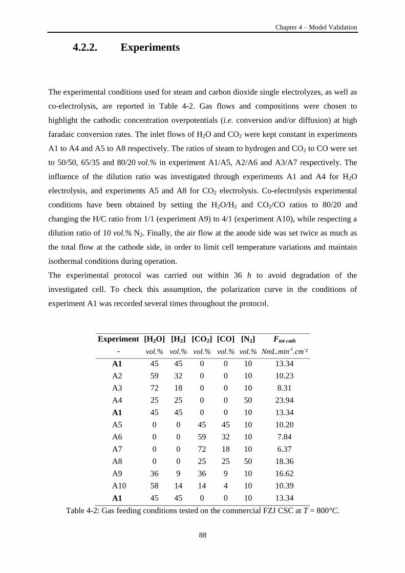
Chapter 4 – Model Validation
88
4.2.2. Experiments
The experimental conditions used for steam and carbon dioxide single electrolyzes, as well as
co-electrolysis, are reported in Table 4-2. Gas flows and compositions were chosen to
highlight the cathodic concentration overpotentials (i.e. conversion and/or diffusion) at high
faradaic conversion rates. The inlet flows of H2O and CO2 were kept constant in experiments
A1 to A4 and A5 to A8 respectively. The ratios of steam to hydrogen and CO2 to CO were set
to 50/50, 65/35 and 80/20 vol.% in experiment A1/A5, A2/A6 and A3/A7 respectively. The
influence of the dilution ratio was investigated through experiments A1 and A4 for H2O
electrolysis, and experiments A5 and A8 for CO2 electrolysis. Co-electrolysis experimental
conditions have been obtained by setting the H2O/H2 and CO2/CO ratios to 80/20 and
changing the H/C ratio from 1/1 (experiment A9) to 4/1 (experiment A10), while respecting a
dilution ratio of 10 vol.% N2. Finally, the air flow at the anode side was set twice as much as
the total flow at the cathode side, in order to limit cell temperature variations and maintain
isothermal conditions during operation.
The experimental protocol was carried out within 36 h to avoid degradation of the
investigated cell. To check this assumption, the polarization curve in the conditions of
experiment A1 was recorded several times throughout the protocol.
Experiment [H2O] [H2] [CO2] [CO] [N2] Ftot cath
- vol.% vol.% vol.% vol.% vol.% NmL.min-1
.cm-²
A1 45 45 0 0 10 13.34
A2 59 32 0 0 10 10.23
A3 72 18 0 0 10 8.31
A4 25 25 0 0 50 23.94
A1 45 45 0 0 10 13.34
A5 0 0 45 45 10 10.20
A6 0 0 59 32 10 7.84
A7 0 0 72 18 10 6.37
A8 0 0 25 25 50 18.36
A9 36 9 36 9 10 16.62
A10 58 14 14 4 10 10.39
A1 45 45 0 0 10 13.34
Table 4-2: Gas feeding conditions tested on the commercial FZJ CSC at T = 800°C.
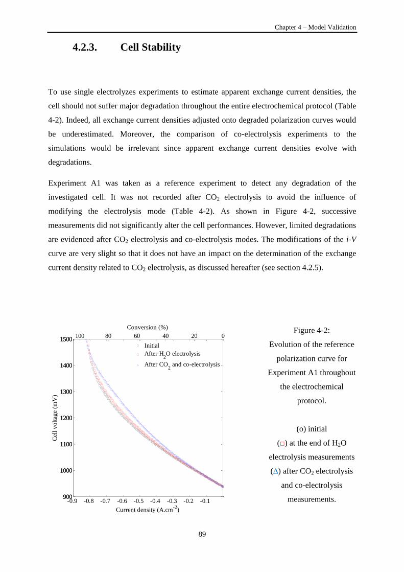
Chapter 4 – Model Validation
89
4.2.3. Cell Stability
To use single electrolyzes experiments to estimate apparent exchange current densities, the
cell should not suffer major degradation throughout the entire electrochemical protocol (Table
4-2). Indeed, all exchange current densities adjusted onto degraded polarization curves would
be underestimated. Moreover, the comparison of co-electrolysis experiments to the
simulations would be irrelevant since apparent exchange current densities evolve with
degradations.
Experiment A1 was taken as a reference experiment to detect any degradation of the
investigated cell. It was not recorded after CO2 electrolysis to avoid the influence of
modifying the electrolysis mode (Table 4-2). As shown in Figure 4-2, successive
measurements did not significantly alter the cell performances. However, limited degradations
are evidenced after CO2 electrolysis and co-electrolysis modes. The modifications of the i-V
curve are very slight so that it does not have an impact on the determination of the exchange
current density related to CO2 electrolysis, as discussed hereafter (see section 4.2.5).
Figure 4-2:
Evolution of the reference
polarization curve for
Experiment A1 throughout
the electrochemical
protocol.
(o) initial
() at the end of H2O
electrolysis measurements
(∆) after CO2 electrolysis
and co-electrolysis
measurements.
-0.9 -0.8 -0.7 -0.6 -0.5 -0.4 -0.3 -0.2 -0.1900
1000
1100
1200
1300
1400
1500
Current density (A.cm-2
)
Cel
l v
olt
age
(mV
)
Initial
After H2O electrolysis
After CO2 and co-electrolysis
020406080100
900
1000
1100
1200
1300
1400
1500
Conversion (%)
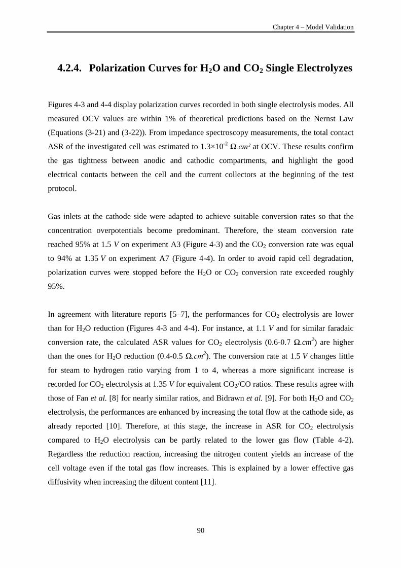
Chapter 4 – Model Validation
90
4.2.4. Polarization Curves for H2O and CO2 Single Electrolyzes
Figures 4-3 and 4-4 display polarization curves recorded in both single electrolysis modes. All
measured OCV values are within 1% of theoretical predictions based on the Nernst Law
(Equations (3-21) and (3-22)). From impedance spectroscopy measurements, the total contact
ASR of the investigated cell was estimated to 1.3×10⁻²
Ω.cm² at OCV. These results confirm
the gas tightness between anodic and cathodic compartments, and highlight the good
electrical contacts between the cell and the current collectors at the beginning of the test
protocol.
Gas inlets at the cathode side were adapted to achieve suitable conversion rates so that the
concentration overpotentials become predominant. Therefore, the steam conversion rate
reached 95% at 1.5 V on experiment A3 (Figure 4-3) and the CO2 conversion rate was equal
to 94% at 1.35 V on experiment A7 (Figure 4-4). In order to avoid rapid cell degradation,
polarization curves were stopped before the H2O or CO2 conversion rate exceeded roughly
95%.
In agreement with literature reports [5–7], the performances for CO2 electrolysis are lower
than for H2O reduction (Figures 4-3 and 4-4). For instance, at 1.1 V and for similar faradaic
conversion rate, the calculated ASR values for CO2 electrolysis (0.6-0.7 Ω.cm2) are higher
than the ones for H2O reduction (0.4-0.5 Ω.cm2). The conversion rate at 1.5 V changes little
for steam to hydrogen ratio varying from 1 to 4, whereas a more significant increase is
recorded for CO2 electrolysis at 1.35 V for equivalent CO2/CO ratios. These results agree with
those of Fan et al. [8] for nearly similar ratios, and Bidrawn et al. [9]. For both H2O and CO2
electrolysis, the performances are enhanced by increasing the total flow at the cathode side, as
already reported [10]. Therefore, at this stage, the increase in ASR for CO2 electrolysis
compared to H2O electrolysis can be partly related to the lower gas flow (Table 4-2).
Regardless the reduction reaction, increasing the nitrogen content yields an increase of the
cell voltage even if the total gas flow increases. This is explained by a lower effective gas
diffusivity when increasing the diluent content [11].
Chapter 4 – Model Validation
91
Figure 4-3: Experimental polarization curves
for experiments A1 to A4 (H2O electrolysis).
Figure 4-4: Experimental polarization curves
for experiments A5 to A8 (CO2 electrolysis).
4.2.5. Determination of Cathodic ‘Apparent’ Exchange
Current Densities 2 2
0,
H H O
cathodei and 2
0,
CO CO
cathodei
Single electrolysis models were used to determine the ‘apparent’ cathodic exchange current
density for both H2O and CO2 electrolysis. For this purpose, the actual microstructural
parameters of the tested cell were used in the simulations (Table 4-1) and the ‘apparent’
anodic exchange current density was set to 200 mA.cm-². This value has been widely used in
SOFC and SOEC studies [12–14] for typical electrodes operated with air at 800°C. In these
conditions, the apparent cathode exchange current densities (related to steam and carbon
dioxide single electrolyzes) remain the only free variables.
-0.8 -0.7 -0.6 -0.5 -0.4 -0.3 -0.2 -0.1 0800
900
1000
1100
1200
1300
1400
1500
Current density (A.cm-2
)
Cel
l v
olt
age
(mV
)
Experiment A1
Experiment A2
Experiment A3
Experiment A4
020406080100
800
900
1000
1100
1200
1300
1400
1500
Conversion (%)
-0.6 -0.5 -0.4 -0.3 -0.2 -0.1 0850
900
950
1000
1050
1100
1150
1200
1250
1300
1350
Current density (A.cm-2
)
Cel
l v
olt
age
(mV
)
Experiment A5
Experiment A6
Experiment A7
Experiment A8
020406080100
850
900
950
1000
1050
1100
1150
1200
1250
1300
1350
Conversion (%)
Chapter 4 – Model Validation
92
4.2.5.1. Steam Electrolysis
Several studies have assessed or used a value in the order of 530 mA.cm-² [3, 15–17] for the
cathodic exchange current density in case of a typical Ni-YSZ electrode operated in steam
electrolysis conditions at 800°C. Using this input value, the steam electrolysis model becomes
entirely predictive. Figure 4-5 displays all simulated polarization curves related to the H2O
electrolysis experimental protocol (experiments A1 to A4) and Figure 4-6 compares
experimental data and simulations for experiment A4. A fair global agreement is found: the
model successfully anticipates OCV, ASR and limiting current densities as well as variations
between the different experimental conditions. As a consequence, the global behavior of the
simulated cell response tends to validate the electrolysis model.
However, a slight difference can be noticed between experimental curves and simulated data
for high current densities (|i| > 0.5 A.cm²), corresponding to high conversion rates (> 60%).
This discrepancy could be due to inaccuracies on the amount of steam effectively reaching the
cell for these experiments. Indeed, uncertainties of 5% have been estimated on steam flow
rates introduced at the cell inlet. That could explain a main part of the difference between
simulated and experimental limiting current densities. Moreover, the mass transfer calculation
across the thick cathode depends on its microstructural properties and gas diffusion
coefficients. A slight error on these parameters could also introduce a bias in the simulations.
The single steam electrolysis model can also be used to adjust any parameter on experimental
data. In order to study the cell response sensitivity on the cathode exchange current density, a
modeling-based approach was developed to fit this parameter on the experimental
polarization curves. It was computed by coupling the single electrolysis model with an error
minimization algorithm focusing solely on the low current density sections of the
experimental data. In this condition, the cell response is mainly governed by activation
overpotentials and not by concentration overpotentials. For each suggested value of 2 2
0,
H H O
cathodei
,
the complete electrochemical module was run iteratively and the corresponding least squares
error was computed and minimized.
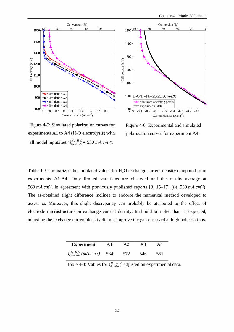
Chapter 4 – Model Validation
93
Figure 4-5: Simulated polarization curves for
experiments A1 to A4 (H2O electrolysis) with
all model inputs set ( 2 2
0,
H H O
cathodei
= 530 mA.cm-²).
Figure 4-6: Experimental and simulated
polarization curves for experiment A4.
Table 4-3 summarizes the simulated values for H2O exchange current density computed from
experiments A1-A4. Only limited variations are observed and the results average at
560 mA.cm-², in agreement with previously published reports [3, 15–17] (i.e. 530 mA.cm
-²).
The as-obtained slight difference inclines to endorse the numerical method developed to
assess i0. Moreover, this slight discrepancy can probably be attributed to the effect of
electrode microstructure on exchange current density. It should be noted that, as expected,
adjusting the exchange current density did not improve the gap observed at high polarizations.
Experiment A1 A2 A3 A4
2 2
0,
H H O
cathodei
(mA.cm-²) 584 572 546 551
Table 4-3: Values for 2 2
0,
H H O
cathodei
adjusted on experimental data.
-0.9 -0.8 -0.7 -0.6 -0.5 -0.4 -0.3 -0.2 -0.1800
900
1000
1100
1200
1300
1400
1500
Current density (A.cm-2
)
Cel
l v
olt
age
(mV
)
Simulation A1
Simulation A2
Simulation A3
Simulation A4
020406080100
800
900
1000
1100
1200
1300
1400
1500
Conversion (%)
-0.9 -0.8 -0.7 -0.6 -0.5 -0.4 -0.3 -0.2 -0.1900
1000
1100
1200
1300
1400
1500
Current density (A.cm-2
)
Cel
l v
olt
age
(mV
)
Simulated operating points
Experimental data
020406080100
900
1000
1100
1200
1300
1400
1500
Conversion (%)
H2O/H2/N2=25/25/50 vol.%
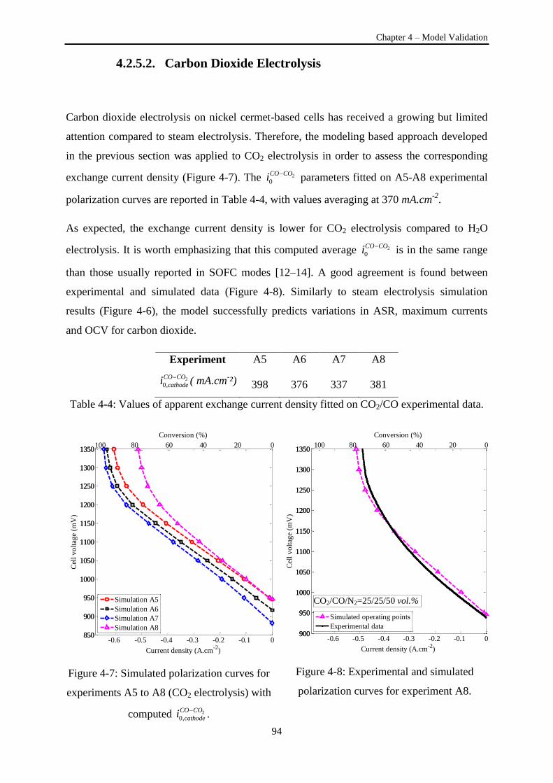
Chapter 4 – Model Validation
94
4.2.5.2. Carbon Dioxide Electrolysis
Carbon dioxide electrolysis on nickel cermet-based cells has received a growing but limited
attention compared to steam electrolysis. Therefore, the modeling based approach developed
in the previous section was applied to CO2 electrolysis in order to assess the corresponding
exchange current density (Figure 4-7). The 2
0
CO COi parameters fitted on A5-A8 experimental
polarization curves are reported in Table 4-4, with values averaging at 370 mA.cm-2
.
As expected, the exchange current density is lower for CO2 electrolysis compared to H2O
electrolysis. It is worth emphasizing that this computed average 2
0
CO COi is in the same range
than those usually reported in SOFC modes [12–14]. A good agreement is found between
experimental and simulated data (Figure 4-8). Similarly to steam electrolysis simulation
results (Figure 4-6), the model successfully predicts variations in ASR, maximum currents
and OCV for carbon dioxide.
Experiment A5 A6 A7 A8
2
0,
CO CO
cathodei ( mA.cm
-²) 398 376 337 381
Table 4-4: Values of apparent exchange current density fitted on CO2/CO experimental data.
Figure 4-7: Simulated polarization curves for
experiments A5 to A8 (CO2 electrolysis) with
computed
2
0,
CO CO
cathodei .
Figure 4-8: Experimental and simulated
polarization curves for experiment A8.
-0.6 -0.5 -0.4 -0.3 -0.2 -0.1 0850
900
950
1000
1050
1100
1150
1200
1250
1300
1350
Current density (A.cm-2
)
Cel
l v
olt
age
(mV
)
Simulation A5
Simulation A6
Simulation A7
Simulation A8
020406080100
850
900
950
1000
1050
1100
1150
1200
1250
1300
1350
Conversion (%)
-0.6 -0.5 -0.4 -0.3 -0.2 -0.1 0900
950
1000
1050
1100
1150
1200
1250
1300
1350
Current density (A.cm-2
)
Cel
l v
olt
age
(mV
)
Simulated operating points
Experimental data
020406080100
900
950
1000
1050
1100
1150
1200
1250
1300
1350
Conversion (%)
CO2/CO/N2=25/25/50 vol.%
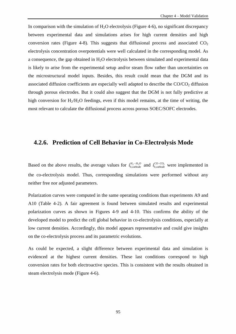
Chapter 4 – Model Validation
95
In comparison with the simulation of H2O electrolysis (Figure 4-6), no significant discrepancy
between experimental data and simulations arises for high current densities and high
conversion rates (Figure 4-8). This suggests that diffusional process and associated CO2
electrolysis concentration overpotentials were well calculated in the corresponding model. As
a consequence, the gap obtained in H2O electrolysis between simulated and experimental data
is likely to arise from the experimental setup and/or steam flow rather than uncertainties on
the microstructural model inputs. Besides, this result could mean that the DGM and its
associated diffusion coefficients are especially well adapted to describe the CO/CO2 diffusion
through porous electrodes. But it could also suggest that the DGM is not fully predictive at
high conversion for H2/H2O feedings, even if this model remains, at the time of writing, the
most relevant to calculate the diffusional process across porous SOEC/SOFC electrodes.
4.2.6. Prediction of Cell Behavior in Co-Electrolysis Mode
Based on the above results, the average values for 2 2
0,
H H O
cathodei and 2
0,
CO CO
cathodei
were implemented in
the co-electrolysis model. Thus, corresponding simulations were performed without any
neither free nor adjusted parameters.
Polarization curves were computed in the same operating conditions than experiments A9 and
A10 (Table 4-2). A fair agreement is found between simulated results and experimental
polarization curves as shown in Figures 4-9 and 4-10. This confirms the ability of the
developed model to predict the cell global behavior in co-electrolysis conditions, especially at
low current densities. Accordingly, this model appears representative and could give insights
on the co-electrolysis process and its parametric evolutions.
As could be expected, a slight difference between experimental data and simulation is
evidenced at the highest current densities. These last conditions correspond to high
conversion rates for both electroactive species. This is consistent with the results obtained in
steam electrolysis mode (Figure 4-6).
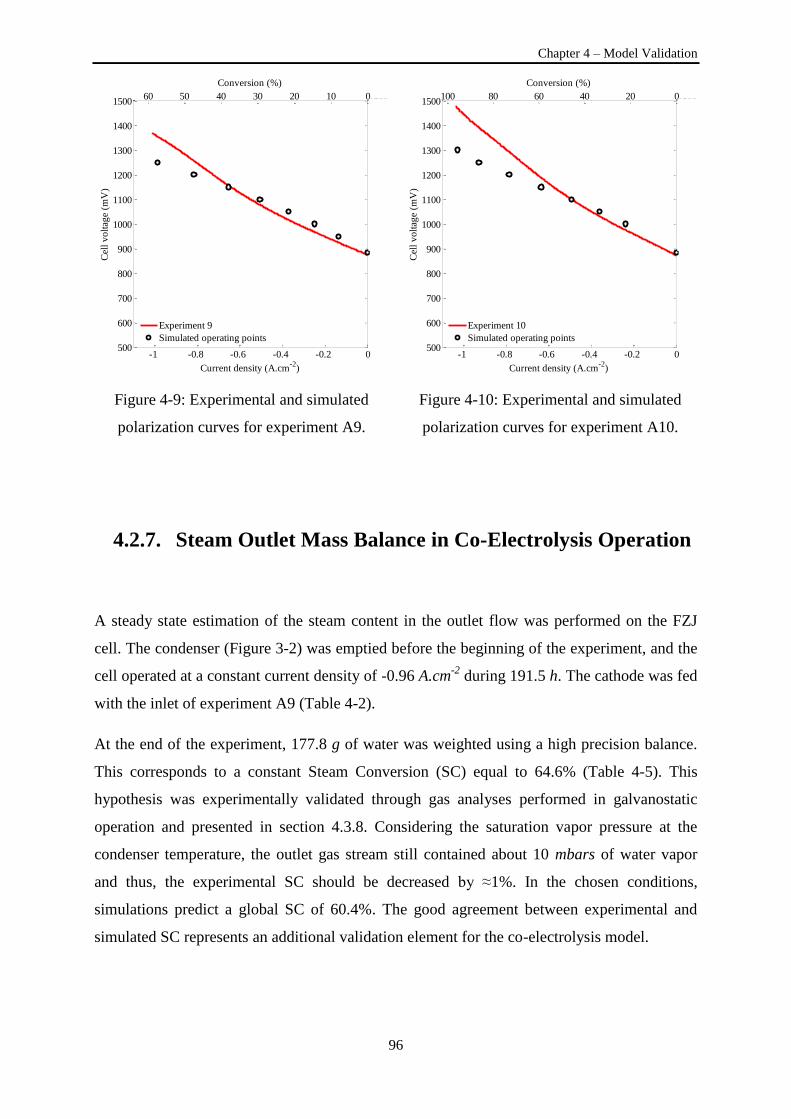
Chapter 4 – Model Validation
96
Figure 4-9: Experimental and simulated
polarization curves for experiment A9.
Figure 4-10: Experimental and simulated
polarization curves for experiment A10.
4.2.7. Steam Outlet Mass Balance in Co-Electrolysis Operation
A steady state estimation of the steam content in the outlet flow was performed on the FZJ
cell. The condenser (Figure 3-2) was emptied before the beginning of the experiment, and the
cell operated at a constant current density of -0.96 A.cm-2
during 191.5 h. The cathode was fed
with the inlet of experiment A9 (Table 4-2).
At the end of the experiment, 177.8 g of water was weighted using a high precision balance.
This corresponds to a constant Steam Conversion (SC) equal to 64.6% (Table 4-5). This
hypothesis was experimentally validated through gas analyses performed in galvanostatic
operation and presented in section 4.3.8. Considering the saturation vapor pressure at the
condenser temperature, the outlet gas stream still contained about 10 mbars of water vapor
and thus, the experimental SC should be decreased by ≈1%. In the chosen conditions,
simulations predict a global SC of 60.4%. The good agreement between experimental and
simulated SC represents an additional validation element for the co-electrolysis model.
-1 -0.8 -0.6 -0.4 -0.2 0500
600
700
800
900
1000
1100
1200
1300
1400
1500
Current density (A.cm-2
)
Cel
l v
olt
age
(mV
)
Experiment 9
Simulated operating points
0102030405060
500
600
700
800
900
1000
1100
1200
1300
1400
1500
Conversion (%)
-1 -0.8 -0.6 -0.4 -0.2 0500
600
700
800
900
1000
1100
1200
1300
1400
1500
Current density (A.cm-2
)
Cel
l v
olt
age
(mV
)
Experiment 10
Simulated operating points
020406080100
500
600
700
800
900
1000
1100
1200
1300
1400
1500
Conversion (%)
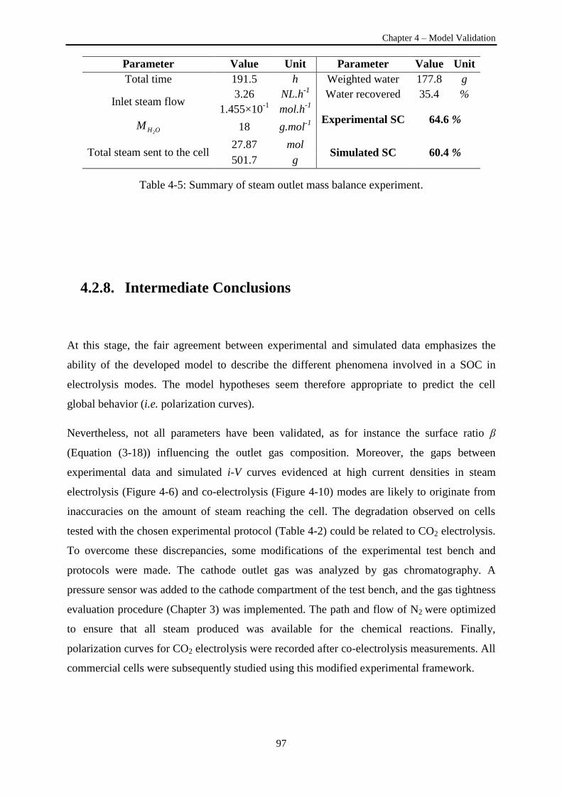
Chapter 4 – Model Validation
97
Parameter Value Unit Parameter Value Unit
Total time 191.5 h Weighted water 177.8 g
Inlet steam flow 3.26 NL.h
-1 Water recovered 35.4 %
1.455×10⁻¹
mol.h-1
Experimental SC 64.6 %
2H OM 18 g.mol-1
Total steam sent to the cell 27.87 mol
Simulated SC 60.4 % 501.7 g
Table 4-5: Summary of steam outlet mass balance experiment.
4.2.8. Intermediate Conclusions
At this stage, the fair agreement between experimental and simulated data emphasizes the
ability of the developed model to describe the different phenomena involved in a SOC in
electrolysis modes. The model hypotheses seem therefore appropriate to predict the cell
global behavior (i.e. polarization curves).
Nevertheless, not all parameters have been validated, as for instance the surface ratio β
(Equation (3-18)) influencing the outlet gas composition. Moreover, the gaps between
experimental data and simulated i-V curves evidenced at high current densities in steam
electrolysis (Figure 4-6) and co-electrolysis (Figure 4-10) modes are likely to originate from
inaccuracies on the amount of steam reaching the cell. The degradation observed on cells
tested with the chosen experimental protocol (Table 4-2) could be related to CO2 electrolysis.
To overcome these discrepancies, some modifications of the experimental test bench and
protocols were made. The cathode outlet gas was analyzed by gas chromatography. A
pressure sensor was added to the cathode compartment of the test bench, and the gas tightness
evaluation procedure (Chapter 3) was implemented. The path and flow of N2 were optimized
to ensure that all steam produced was available for the chemical reactions. Finally,
polarization curves for CO2 electrolysis were recorded after co-electrolysis measurements. All
commercial cells were subsequently studied using this modified experimental framework.
Chapter 4 – Model Validation
98
4.3. Investigations of a CSC with Unknown
Microstructure (Optimized Cell)
4.3.1. Methodology
A second commercial CSC was tested to further validate the co-electrolysis model. However,
contrary to the previous FZJ cell, the electrodes microstructure was unknown. Therefore,
Scanning Electron Microscopy (SEM) examinations were performed and polarization curves
were recorded in single electrolysis modes to assess the cathode support layer microstructure
parameters (porosity, tortuosity factor and mean pore diameter) and ‘apparent’ exchange
current densities ( 2
0,
CO CO
cathodei , 2 2
0,
H O H
cathodei and
0,anodei ).
4.3.2. Cell
The cell consisted of a thick Ni-8YSZ cathode (thickness 500 µm, diameter 50 mm), a thin
8YSZ electrolyte (5 µm), an intermediate layer of CGO (2 µm), and a LSC anode (20 µm).
The anode was 20 mm in diameter so that the electroactive cell area was 3.14 cm².
The cermet porosity was evaluated to 0.46 by manual segmentation (with ImageJ software) of
a polished cross section image (Figure 4-11). It was obtained with a Scanning Electron
Microscopy in Back Scattering Electron mode using a Philips XL30 scanning electron
microscope complemented by a Si-Li Oxford Instruments Detector. Additionally, the mean
pore radius was estimated to about 1.2 µm.
Chapter 4 – Model Validation
99
Figure 4-11:
SEM cross-section examination of
the commercial cermet.
A thin Ni layer, probably used to
improve electrical contact, is
observed on this micrograph.
4.3.3. Experiments
Initial performances of the investigated CSC were recorded at 800°C in steam electrolysis, co-
electrolysis and CO2 electrolysis modes. Experimental conditions of the chosen protocol are
given in Table 4-6. For each experiment, the corresponding polarization curve was recorded.
All low and high flow rates experiments display respectively the same initial amount of
oxidized species (i.e. H2O and/or CO2). Thus, performances in the different modes can be
directly compared since gas conversions will be equal at a given current density. The overall
protocol was carried out in 12 h to limit cell degradation. To check the cell performance
stability, the polarization curve corresponding to Experiment B1 was recorded after each
mode change. It should be emphasized that the maximum variation recorded between
experimental OCV and Nernst law predictions was merely 0.4%.
The cathode outlet gas composition corresponding to Experiment B3* was investigated by
µGC as a function of the current density. Therefore, the molar fractions of H2, N2, O2, CH4,
CO and CO2 were measured at OCV, -0.48, -0.96, -1.43 and -1.75 A.cm-2
, respectively.
Additionally, the WGS reaction kinetics implemented in the model was validated through gas
analyses at OCV. Finally, the evolution of the outlet composition in steady state operation
was investigated over 288 h.
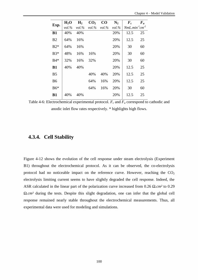
Chapter 4 – Model Validation
100
Exp. H2O H2 CO2 CO N2 Fc Fa
vol.% vol.% vol.% vol.% vol.% NmL.min-1
cm-2
B1 40% 40%
20% 12.5 25
B2 64% 16%
20% 12.5 25
B2* 64% 16%
20% 30 60
B3* 48% 16% 16%
20% 30 60
B4* 32% 16% 32%
20% 30 60
B1 40% 40%
20% 12.5 25
B5
40% 40% 20% 12.5 25
B6
64% 16% 20% 12.5 25
B6*
64% 16% 20% 30 60
B1 40% 40%
20% 12.5 25
Table 4-6: Electrochemical experimental protocol. Fc and Fa correspond to cathodic and
anodic inlet flow rates respectively. * highlights high flows.
4.3.4. Cell Stability
Figure 4-12 shows the evolution of the cell response under steam electrolysis (Experiment
B1) throughout the electrochemical protocol. As it can be observed, the co-electrolysis
protocol had no noticeable impact on the reference curve. However, reaching the CO2
electrolysis limiting current seems to have slightly degraded the cell response. Indeed, the
ASR calculated in the linear part of the polarization curve increased from 0.26 Ω.cm² to 0.29
Ω.cm² during the tests. Despite this slight degradation, one can infer that the global cell
response remained nearly stable throughout the electrochemical measurements. Thus, all
experimental data were used for modeling and simulations.
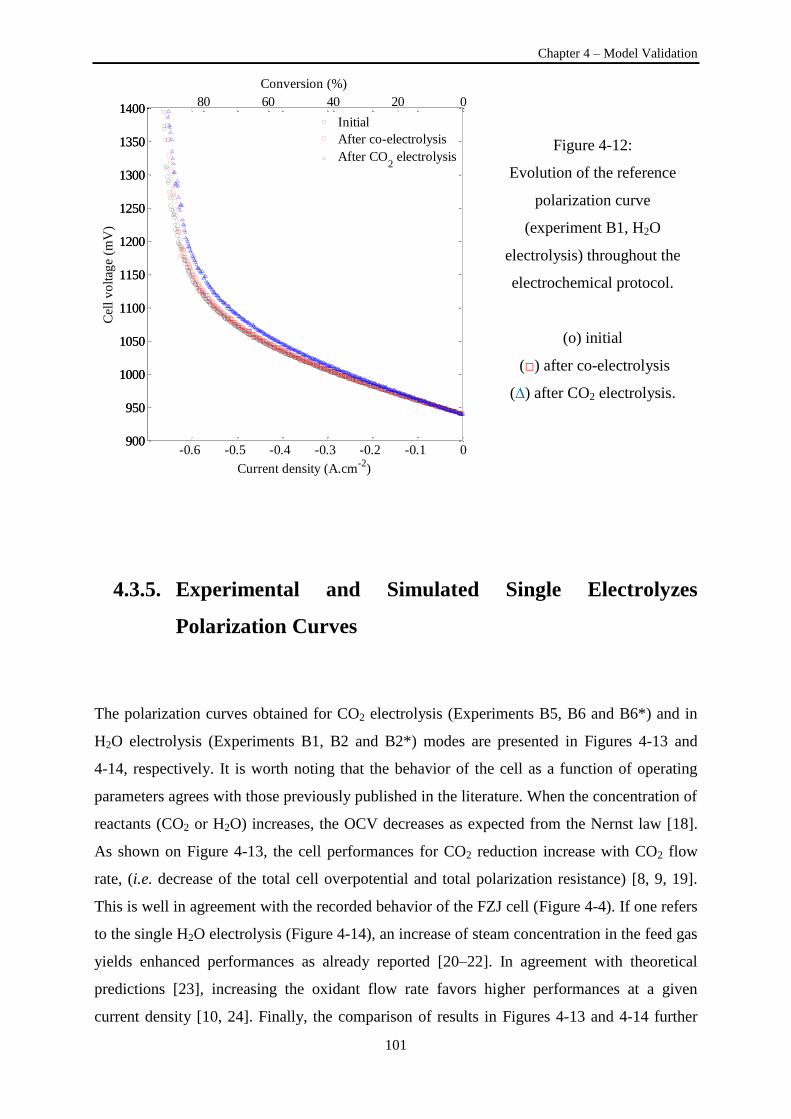
Chapter 4 – Model Validation
101
Figure 4-12:
Evolution of the reference
polarization curve
(experiment B1, H2O
electrolysis) throughout the
electrochemical protocol.
(o) initial
() after co-electrolysis
(∆) after CO2 electrolysis.
4.3.5. Experimental and Simulated Single Electrolyzes
Polarization Curves
The polarization curves obtained for CO2 electrolysis (Experiments B5, B6 and B6*) and in
H2O electrolysis (Experiments B1, B2 and B2*) modes are presented in Figures 4-13 and
4-14, respectively. It is worth noting that the behavior of the cell as a function of operating
parameters agrees with those previously published in the literature. When the concentration of
reactants (CO2 or H2O) increases, the OCV decreases as expected from the Nernst law [18].
As shown on Figure 4-13, the cell performances for CO2 reduction increase with CO2 flow
rate, (i.e. decrease of the total cell overpotential and total polarization resistance) [8, 9, 19].
This is well in agreement with the recorded behavior of the FZJ cell (Figure 4-4). If one refers
to the single H2O electrolysis (Figure 4-14), an increase of steam concentration in the feed gas
yields enhanced performances as already reported [20–22]. In agreement with theoretical
predictions [23], increasing the oxidant flow rate favors higher performances at a given
current density [10, 24]. Finally, the comparison of results in Figures 4-13 and 4-14 further
-0.6 -0.5 -0.4 -0.3 -0.2 -0.1 0900
950
1000
1050
1100
1150
1200
1250
1300
1350
1400
Current density (A.cm-2
)
Cel
l v
olt
age
(mV
)
Initial
After co-electrolysis
After CO2 electrolysis
020406080
900
950
1000
1050
1100
1150
1200
1250
1300
1350
1400
Conversion (%)

Chapter 4 – Model Validation
102
confirms that lower current densities are recorded for CO2 electrolysis compared to H2O
electrolysis, which agrees with literature reports [5–7], and previous results obtained with the
FZJ cell (cf. section 4.2).
The following aims at assessing the electrokinetic parameters of all three electrochemical
reactions (Equations (3-1) to (3-3)) related to the cell considered, as well as the unknown
microstructure parameters.
The anode was modeled using usual values of microstructural parameters, as reported in the
literature [3] and already implemented in section 4.2. It should be noted that these parameters
have a limited influence on the cell global response. Indeed, under air sweeping (i.e. 2
0int_i
Oy ),
if the produced oxygen transport through the electrode were to be extremely hindered by the
microstructure so that 2
_ 0 1int i
Oy , the corresponding concentration overpotential should be
limited to 36 mV (cf. Equation (3-32)).
4.3.5.1. Determination of Cathode Tortuosity Factor and 2
0,
CO CO
cathodei
Since the cathode porosity and mean pore radius were assessed (cf. section 4.3.2), only the
cathodic tortuosity factor, which largely controls the limiting currents, remains to be adjusted
on experimental data at high cell polarization. Since the model can accurately predict the CO2
electrolysis response (Figure 4-8), c was firstly determined by fitting simulations on
polarization curves of experiments B5 and B6 to grasp limiting currents.
The ‘apparent’ exchange current densities 2
0,
CO CO
cathodei and 0,anodei were then tuned to be
representative of the cell ASR (Table 4-7). It is worth mentioning that the as-obtained values
are higher by a factor 4 than literature reports [15, 25, 26]. However, one must keep in mind
that these values are ‘apparent’ macroscopic descriptions of microscopic mechanisms which
strongly depend on microstructure. Consequently, a higher exchange current density can be
expected for an optimized functional layer exhibiting a higher density of TPBl. For the
investigated cell, a sensitivity analysis was performed to quantify the influence of i0 on the
simulated response (cf. section 4.3.10).
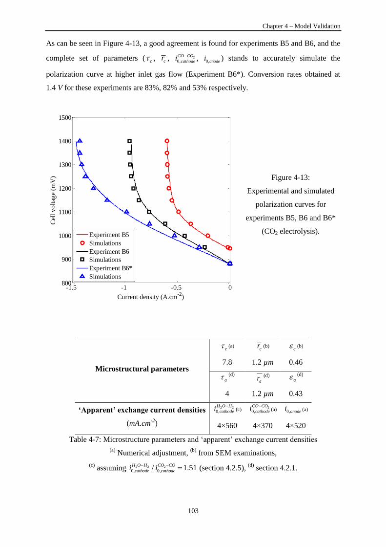
Chapter 4 – Model Validation
103
As can be seen in Figure 4-13, a good agreement is found for experiments B5 and B6, and the
complete set of parameters ( c , cr , 2
0,
CO CO
cathodei , 0,anodei ) stands to accurately simulate the
polarization curve at higher inlet gas flow (Experiment B6*). Conversion rates obtained at
1.4 V for these experiments are 83%, 82% and 53% respectively.
Figure 4-13:
Experimental and simulated
polarization curves for
experiments B5, B6 and B6*
(CO2 electrolysis).
Microstructural parameters
c (a) cr (b)
c (b)
7.8 1.2 µm 0.46
a(d)
ar
(d) a
(d)
4 1.2 µm 0.43
‘Apparent’ exchange current densities
(mA.cm-2
)
2 2
0,
H O H
cathodei
(c) 2
0,
CO CO
cathodei (a) 0,anodei (a)
4×560 4×370 4×520
Table 4-7: Microstructure parameters and ‘apparent’ exchange current densities
(a) Numerical adjustment,
(b) from SEM examinations,
(c) assuming 2 2 2
0, 0,/ 1.51H O H CO CO
cathode cathodei i (section 4.2.5),
(d) section 4.2.1.
-1.5 -1 -0.5 0800
900
1000
1100
1200
1300
1400
1500
Current density (A.cm-2
)
Cel
l v
olt
age
(mV
)
Experiment B5
Simulations
Experiment B6
Simulations
Experiment B6*
Simulations

Chapter 4 – Model Validation
104
4.3.5.2. Determination of 2 2
0,
H H O
cathodei
The ratio of electrochemical oxidation rates of H2 to that of CO was reported to be in the
range of 2-2.5 at 800°C [27]. It was then suggested to use such values to express
2 2 2 2
0 0, 0,
H O H CO CO
cathode cathodeR i i [25]. As done for the FZJ cell (section 4.2),
0R was evaluated to 1.51
from experimental polarization curves. This value was thus kept constant in this section,
leading to 2 2 2
0 4 560 .H H Oi mAcm . Therefore, no further adjustments were made to simulate
steam electrolysis.
As for carbon dioxide electrolysis (Figure 4-13), a global agreement is evidenced between
experimental and simulated results (Figure 4-14). Modeling predicts both OCV and ASR
variations when the inlet composition and/or flow are modified. However, the simulations
seem to overestimate limiting current densities for H2O electrolysis, as previously observed
for the FZJ cell (Figure 4-6). The gap is evidenced at high conversion rates when hydrogen
becomes predominant in the gas phase. This could be partly related to uncertainties
concerning the amount of steam effectively reaching the cell. But on may also evoke the
ability of the DGM relevance to model H2/H2O transport in SOEC at high polarizations, when
H2 is preponderant. Indeed, the effective Knudsen diffusion of hydrogen is 3-5 times larger
than for the other components, and the effective binary diffusion coefficient of steam in
hydrogen is 5.5 times higher than that of CO2 in CO [28, 29]. In other words, in the as-
modeled H2O electrolysis (i.e. constant 2 2
0
H H Oi ), diffusion of H2 (i.e. through DGM, diffusion
coefficients, etc.) is largely enhanced compared to the other gaseous components.
Nevertheless, it can be concluded that both single electrolysis models can simulate the global
cell response with the set of microstructure parameters and ‘apparent’ exchange current
densities implemented.
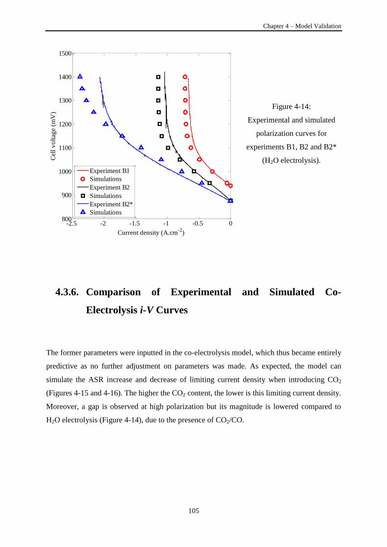
Chapter 4 – Model Validation
105
Figure 4-14:
Experimental and simulated
polarization curves for
experiments B1, B2 and B2*
(H2O electrolysis).
4.3.6. Comparison of Experimental and Simulated Co-
Electrolysis i-V Curves
The former parameters were inputted in the co-electrolysis model, which thus became entirely
predictive as no further adjustment on parameters was made. As expected, the model can
simulate the ASR increase and decrease of limiting current density when introducing CO2
(Figures 4-15 and 4-16). The higher the CO2 content, the lower is this limiting current density.
Moreover, a gap is observed at high polarization but its magnitude is lowered compared to
H2O electrolysis (Figure 4-14), due to the presence of CO2/CO.
-2.5 -2 -1.5 -1 -0.5 0800
900
1000
1100
1200
1300
1400
1500
Current density (A.cm-2
)
Cel
l v
olt
age
(mV
)
Experiment B1
Simulations
Experiment B2
Simulations
Experiment B2*
Simulations

Chapter 4 – Model Validation
106
Figure 4-15: Experimental and simulated
polarization curves for experiment B3*.
Figure 4-16: Experimental and simulated
polarization curves for experiment B4*.
This first step of model validation is based on comparisons between experimental and
simulated polarization curves. Therefore, only the global cell response is compared to the
simulations. Additional experiments are thus required to further extend the range of use of the
co-electrolysis model. Consequently, the following sections aim at validating, on one hand,
the WGS reaction kinetics implemented in the model and, on the other hand, the model ability
to predict co-electrolysis outlet compositions under operation.
4.3.7. Gas Analyses – WGSR Kinetics Validation
Four water gas Shift reaction Experiments (SExp., Table 4-8) were performed to validate the
kinetics of the WGS reaction implemented in the model (cf. Table 3-4). In order to increase
the experimental accuracy, the inlet gas flows were significantly higher than those used in the
previous protocols (Tables 4-2 and 4-6). Gas analyses were carried out on the gaseous outlets
at OCV and 800°C. Compositions for SExp.1 to 3 were compatible with a co-electrolysis
-2.5 -2 -1.5 -1 -0.5 0800
900
1000
1100
1200
1300
1400
1500
Current density (A.cm-2
)
Cel
l v
olt
age
(mV
)
Experiment B3*
Simulated operating points
020406080
800
900
1000
1100
1200
1300
1400
1500
Conversion (%)
-2.5 -2 -1.5 -1 -0.5 0800
900
1000
1100
1200
1300
1400
1500
Current density (A.cm-2
)
Cel
l v
olt
age
(mV
)
Experiment B4*
Simulated operating points
020406080
800
900
1000
1100
1200
1300
1400
1500
Conversion (%)
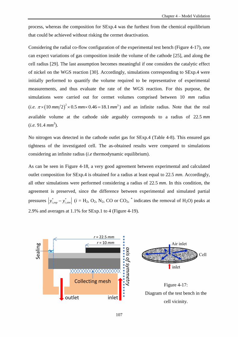
Chapter 4 – Model Validation
107
process, whereas the composition for SExp.4 was the furthest from the chemical equilibrium
that could be achieved without risking the cermet deactivation.
Considering the radial co-flow configuration of the experimental test bench (Figure 4-17), one
can expect variations of gas composition inside the volume of the cathode [25], and along the
cell radius [29]. The last assumption becomes meaningful if one considers the catalytic effect
of nickel on the WGS reaction [30]. Accordingly, simulations corresponding to SExp.4 were
initially performed to quantify the volume required to be representative of experimental
measurements, and thus evaluate the rate of the WGS reaction. For this purpose, the
simulations were carried out for cermet volumes comprised between 10 mm radius
(i.e. 2 310 2 0.5 0.46 18.1mm mm mm ) and an infinite radius. Note that the real
available volume at the cathode side arguably corresponds to a radius of 22.5 mm
(i.e. 91.4 mm3).
No nitrogen was detected in the cathode outlet gas for SExp.4 (Table 4-8). This ensured gas
tightness of the investigated cell. The as-obtained results were compared to simulations
considering an infinite radius (i.e thermodynamic equilibrium).
As can be seen in Figure 4-18, a very good agreement between experimental and calculated
outlet composition for SExp.4 is obtained for a radius at least equal to 22.5 mm. Accordingly,
all other simulations were performed considering a radius of 22.5 mm. In this condition, the
agreement is preserved, since the difference between experimental and simulated partial
pressures * *
, ,i exp i simy y (i = H2, O2, N2, CO or CO2, * indicates the removal of H2O) peaks at
2.9% and averages at 1.1% for SExp.1 to 4 (Figure 4-19).
Figure 4-17:
Diagram of the test bench in the
cell vicinity.
axis o
f symm
etry
r = 10 mm
r = 22.5 mm
inletoutlet
Seal
ing
Collecting mesh
inlet
Air inlet
Cell
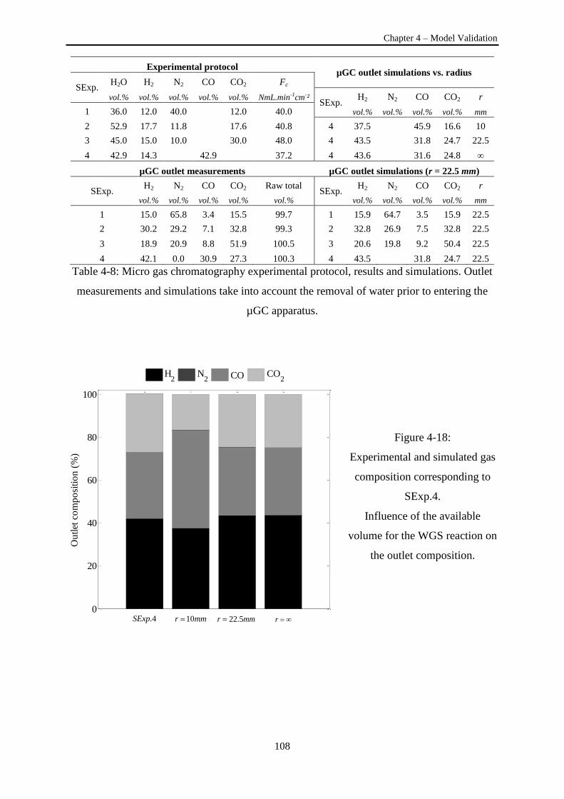
Chapter 4 – Model Validation
108
Experimental protocol µGC outlet simulations vs. radius
SExp. H2O H2 N2 CO CO2 Fc
vol.% vol.% vol.% vol.% vol.% NmL.min-1cm-² SExp.
H2 N2 CO CO2 r
1 36.0 12.0 40.0
12.0 40.0 vol.% vol.% vol.% vol.% mm
2 52.9 17.7 11.8
17.6 40.8 4 37.5 45.9 16.6 10
3 45.0 15.0 10.0
30.0 48.0 4 43.5 31.8 24.7 22.5
4 42.9 14.3
42.9
37.2 4 43.6 31.6 24.8 ∞
µGC outlet measurements µGC outlet simulations (r = 22.5 mm)
SExp. H2 N2 CO CO2 Raw total
SExp. H2 N2 CO CO2 r
vol.% vol.% vol.% vol.% vol.% vol.% vol.% vol.% vol.% mm
1 15.0 65.8 3.4 15.5 99.7 1 15.9 64.7 3.5 15.9 22.5
2 30.2 29.2 7.1 32.8 99.3 2 32.8 26.9 7.5 32.8 22.5
3 18.9 20.9 8.8 51.9 100.5 3 20.6 19.8 9.2 50.4 22.5
4 42.1 0.0 30.9 27.3 100.3 4 43.5 31.8 24.7 22.5
Table 4-8: Micro gas chromatography experimental protocol, results and simulations. Outlet
measurements and simulations take into account the removal of water prior to entering the
µGC apparatus.
Figure 4-18:
Experimental and simulated gas
composition corresponding to
SExp.4.
Influence of the available
volume for the WGS reaction on
the outlet composition.
0
20
40
60
80
100
SExp.4 r=10mm r=22.5mm r=
Ou
tlet
co
mp
osi
tio
n (
%)
H2
N2 CO CO
2
.4SExp 10r mm 22.5r mm r
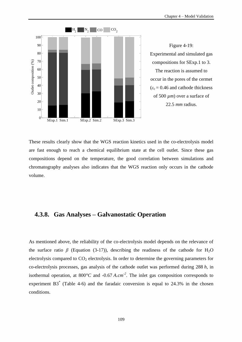
Chapter 4 – Model Validation
109
Figure 4-19:
Experimental and simulated gas
compositions for SExp.1 to 3.
The reaction is assumed to
occur in the pores of the cermet
(εc = 0.46 and cathode thickness
of 500 µm) over a surface of
22.5 mm radius.
These results clearly show that the WGS reaction kinetics used in the co-electrolysis model
are fast enough to reach a chemical equilibrium state at the cell outlet. Since these gas
compositions depend on the temperature, the good correlation between simulations and
chromatography analyses also indicates that the WGS reaction only occurs in the cathode
volume.
4.3.8. Gas Analyses – Galvanostatic Operation
As mentioned above, the reliability of the co-electrolysis model depends on the relevance of
the surface ratio β (Equation (3-17)), describing the readiness of the cathode for H2O
electrolysis compared to CO2 electrolysis. In order to determine the governing parameters for
co-electrolysis processes, gas analysis of the cathode outlet was performed during 288 h, in
isothermal operation, at 800°C and -0.67 A.cm-2
. The inlet gas composition corresponds to
experiment B3* (Table 4-6) and the faradaic conversion is equal to 24.3% in the chosen
conditions.
SExp.1 Sim.1 SExp.2 Sim.2 SExp.3 Sim.3 0
10
20
30
40
50
60
70
80
90
100
Ou
tlet
co
mp
osi
tio
n (
%)
H2
N2 CO CO
2
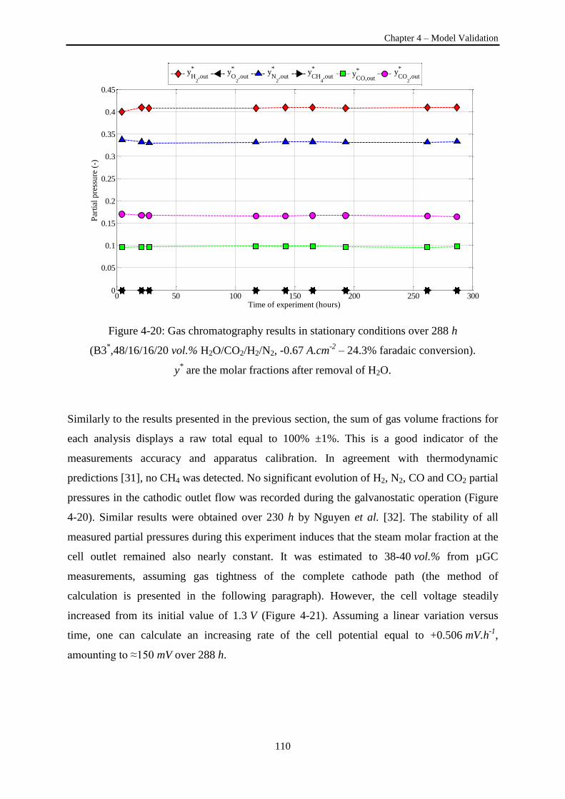
Chapter 4 – Model Validation
110
Figure 4-20: Gas chromatography results in stationary conditions over 288 h
(B3*,48/16/16/20 vol.% H2O/CO2/H2/N2, -0.67 A.cm
-2 – 24.3% faradaic conversion).
y* are the molar fractions after removal of H2O.
Similarly to the results presented in the previous section, the sum of gas volume fractions for
each analysis displays a raw total equal to 100% ±1%. This is a good indicator of the
measurements accuracy and apparatus calibration. In agreement with thermodynamic
predictions [31], no CH4 was detected. No significant evolution of H2, N2, CO and CO2 partial
pressures in the cathodic outlet flow was recorded during the galvanostatic operation (Figure
4-20). Similar results were obtained over 230 h by Nguyen et al. [32]. The stability of all
measured partial pressures during this experiment induces that the steam molar fraction at the
cell outlet remained also nearly constant. It was estimated to 38-40 vol.% from µGC
measurements, assuming gas tightness of the complete cathode path (the method of
calculation is presented in the following paragraph). However, the cell voltage steadily
increased from its initial value of 1.3 V (Figure 4-21). Assuming a linear variation versus
time, one can calculate an increasing rate of the cell potential equal to +0.506 mV.h-1
,
amounting to ≈150 mV over 288 h.
0 50 100 150 200 250 3000
0.05
0.1
0.15
0.2
0.25
0.3
0.35
0.4
0.45
Time of experiment (hours)
Par
tial
pre
ssu
re (
-)
yH
2,out
*y
O2,out
*y
N2,out
*y
CH4,out
*y
CO,out
* yCO
2,out
*
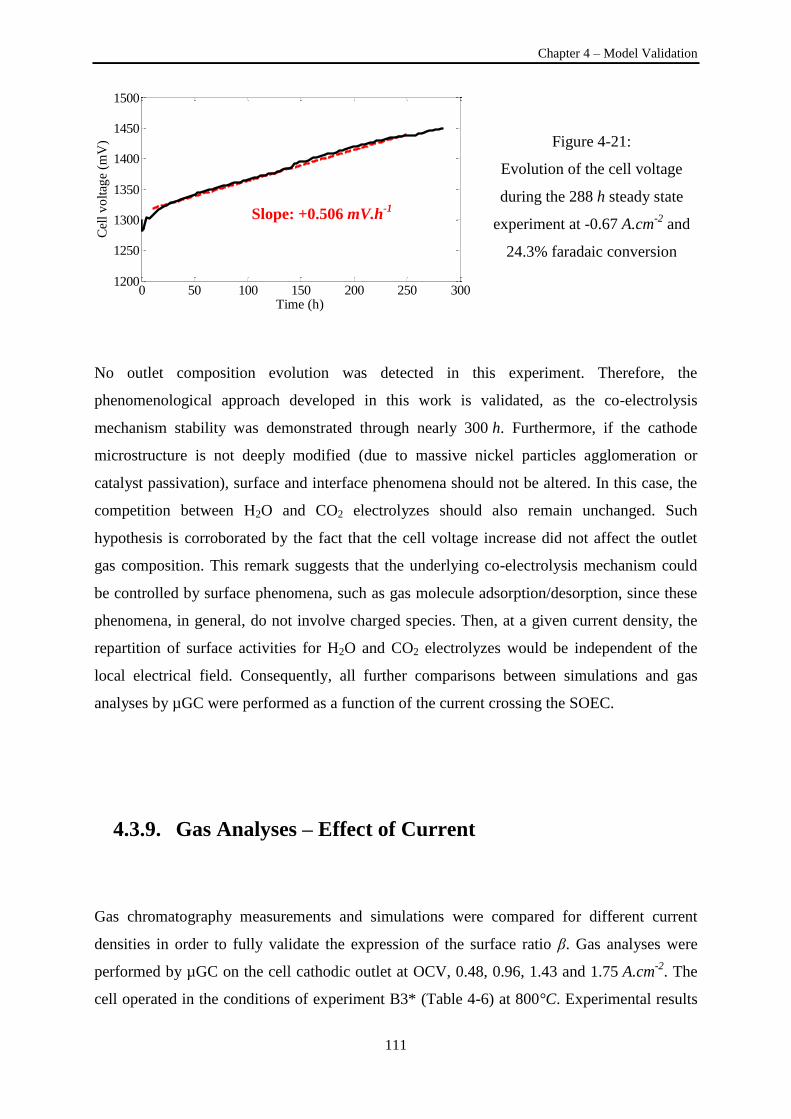
Chapter 4 – Model Validation
111
Figure 4-21:
Evolution of the cell voltage
during the 288 h steady state
experiment at -0.67 A.cm-2
and
24.3% faradaic conversion
No outlet composition evolution was detected in this experiment. Therefore, the
phenomenological approach developed in this work is validated, as the co-electrolysis
mechanism stability was demonstrated through nearly 300 h. Furthermore, if the cathode
microstructure is not deeply modified (due to massive nickel particles agglomeration or
catalyst passivation), surface and interface phenomena should not be altered. In this case, the
competition between H2O and CO2 electrolyzes should also remain unchanged. Such
hypothesis is corroborated by the fact that the cell voltage increase did not affect the outlet
gas composition. This remark suggests that the underlying co-electrolysis mechanism could
be controlled by surface phenomena, such as gas molecule adsorption/desorption, since these
phenomena, in general, do not involve charged species. Then, at a given current density, the
repartition of surface activities for H2O and CO2 electrolyzes would be independent of the
local electrical field. Consequently, all further comparisons between simulations and gas
analyses by µGC were performed as a function of the current crossing the SOEC.
4.3.9. Gas Analyses – Effect of Current
Gas chromatography measurements and simulations were compared for different current
densities in order to fully validate the expression of the surface ratio β. Gas analyses were
performed by µGC on the cell cathodic outlet at OCV, 0.48, 0.96, 1.43 and 1.75 A.cm-2
. The
cell operated in the conditions of experiment B3* (Table 4-6) at 800°C. Experimental results
0 50 100 150 200 250 3001200
1250
1300
1350
1400
1450
1500
Time (h)
Cel
l v
olt
age
(mV
)
Slope: +0.506 mV.h-1
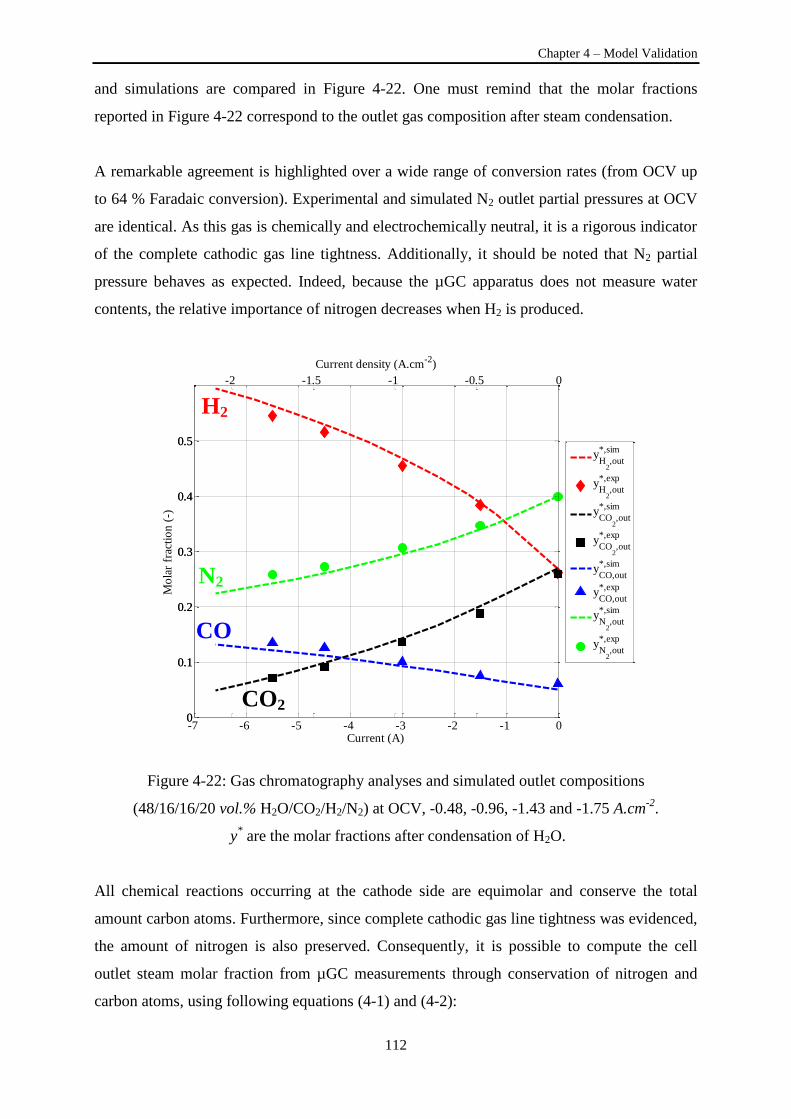
Chapter 4 – Model Validation
112
and simulations are compared in Figure 4-22. One must remind that the molar fractions
reported in Figure 4-22 correspond to the outlet gas composition after steam condensation.
A remarkable agreement is highlighted over a wide range of conversion rates (from OCV up
to 64 % Faradaic conversion). Experimental and simulated N2 outlet partial pressures at OCV
are identical. As this gas is chemically and electrochemically neutral, it is a rigorous indicator
of the complete cathodic gas line tightness. Additionally, it should be noted that N2 partial
pressure behaves as expected. Indeed, because the µGC apparatus does not measure water
contents, the relative importance of nitrogen decreases when H2 is produced.
Figure 4-22: Gas chromatography analyses and simulated outlet compositions
(48/16/16/20 vol.% H2O/CO2/H2/N2) at OCV, -0.48, -0.96, -1.43 and -1.75 A.cm-2
.
y* are the molar fractions after condensation of H2O.
All chemical reactions occurring at the cathode side are equimolar and conserve the total
amount carbon atoms. Furthermore, since complete cathodic gas line tightness was evidenced,
the amount of nitrogen is also preserved. Consequently, it is possible to compute the cell
outlet steam molar fraction from µGC measurements through conservation of nitrogen and
carbon atoms, using following equations (4-1) and (4-2):
-7 -6 -5 -4 -3 -2 -1 00
0.1
0.2
0.3
0.4
0.5
Current (A)
Mo
lar
frac
tio
n (
-)
yH
2,out
*,sim
yH
2,out
*,exp
yCO
2,out
*,sim
yCO
2,out
*,exp
yCO,out
*,sim
yCO,out
*,exp
yN
2,out
*,sim
yN
2,out
*,exp
-2 -1.5 -1 -0.5 0
0
0.1
0.2
0.3
0.4
0.5
Current density (A.cm-2
)
H2
CO2
CO
N2
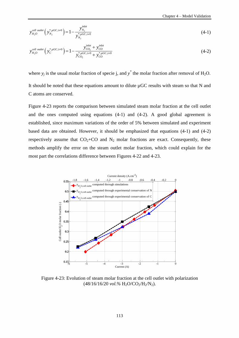
Chapter 4 – Model Validation
113
2
2 2
2
*, , 0
*, , 01
inlet
Ncell outlet µGC i
H O N µGC i
N
yy y
y
(4-1)
2
2
2
*, , 0
*, , 0 *, , 01
inlet inlet
CO COcell outlet µGC i
H O C µGC i µGC i
CO CO
y yy y
y y
(4-2)
where yj is the usual molar fraction of specie j, and y* the molar fraction after removal of H2O.
It should be noted that these equations amount to dilute µGC results with steam so that N and
C atoms are conserved.
Figure 4-23 reports the comparison between simulated steam molar fraction at the cell outlet
and the ones computed using equations (4-1) and (4-2). A good global agreement is
established, since maximum variations of the order of 5% between simulated and experiment
based data are obtained. However, it should be emphasized that equations (4-1) and (4-2)
respectively assume that CO2+CO and N2 molar fractions are exact. Consequently, these
methods amplify the error on the steam outlet molar fraction, which could explain for the
most part the correlations difference between Figures 4-22 and 4-23.
Figure 4-23: Evolution of steam molar fraction at the cell outlet with polarization
(48/16/16/20 vol.% H2O/CO2/H2/N2).
-6 -5 -4 -3 -2 -1 00.15
0.2
0.25
0.3
0.35
0.4
0.45
0.5
0.55
Current (A)
Cel
l o
utl
et H
2O
mo
lar
frac
tio
n (
-)
yH
2O,cell outlet
computed through simulations
yH
2O,cell outlet
computed through experimental conservation of N
yH
2O,cell outlet
computed through experimental conservation of C
-1.8 -1.6 -1.4 -1.2 -1 -0.8 -0.6 -0.4 -0.2 0
0.15
0.2
0.25
0.3
0.35
0.4
0.45
0.5
0.55
Current density (A.cm-2
)
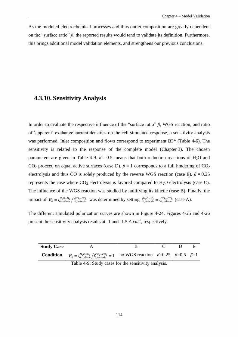
Chapter 4 – Model Validation
114
As the modeled electrochemical processes and thus outlet composition are greatly dependent
on the “surface ratio” β, the reported results would tend to validate its definition. Furthermore,
this brings additional model validation elements, and strengthens our previous conclusions.
4.3.10. Sensitivity Analysis
In order to evaluate the respective influence of the “surface ratio” β, WGS reaction, and ratio
of ‘apparent’ exchange current densities on the cell simulated response, a sensitivity analysis
was performed. Inlet composition and flows correspond to experiment B3* (Table 4-6). The
sensitivity is related to the response of the complete model (Chapter 3). The chosen
parameters are given in Table 4-9. β = 0.5 means that both reduction reactions of H2O and
CO2 proceed on equal active surfaces (case D). β = 1 corresponds to a full hindering of CO2
electrolysis and thus CO is solely produced by the reverse WGS reaction (case E). β = 0.25
represents the case where CO2 electrolysis is favored compared to H2O electrolysis (case C).
The influence of the WGS reaction was studied by nullifying its kinetic (case B). Finally, the
impact of 2 2 2 2
0 0, 0,
H O H CO CO
cathode cathodeR i i was determined by setting 2 2 2 2
0, 0,
H O H CO CO
cathode cathodei i
(case A).
The different simulated polarization curves are shown in Figure 4-24. Figures 4-25 and 4-26
present the sensitivity analysis results at -1 and -1.5 A.cm-2
, respectively.
Study Case A B C D E
Condition 2 2 2 2
0 0, 0, 1H O H CO CO
cathode cathodeR i i
no WGS reaction β=0.25 β=0.5 β=1
Table 4-9: Study cases for the sensitivity analysis.
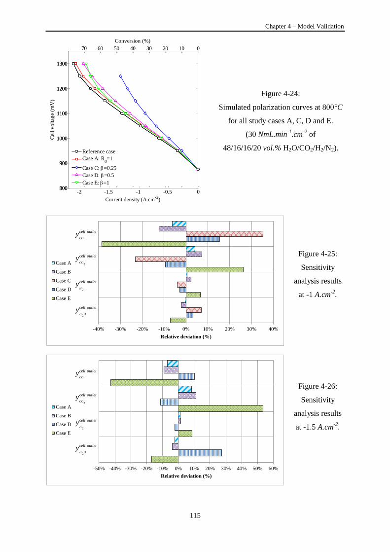
Chapter 4 – Model Validation
115
Figure 4-24:
Simulated polarization curves at 800°C
for all study cases A, C, D and E.
(30 NmL.min-1
.cm-2
of
48/16/16/20 vol.% H2O/CO2/H2/N2).
Figure 4-25:
Sensitivity
analysis results
at -1 A.cm-2
.
Figure 4-26:
Sensitivity
analysis results
at -1.5 A.cm-2
.
-2 -1.5 -1 -0.5 0800
900
1000
1100
1200
1300
Current density (A.cm-2
)
Cel
l v
olt
age
(mV
)
Reference case
Case A: R0=1
Case C: =0.25
Case D: =0.5
Case E: =1
010203040506070
800
900
1000
1100
1200
1300
Conversion (%)
-40% -30% -20% -10% 0% 10% 20% 30% 40%
P_H2O,out
P_H2s
P_CO2s
P_COs
Relative deviation (%)
Case A
Case B
Case C
Case D
Case E
2
H O
cell outlety
2
H
cell outlety
2
CO
cell outlety
CO
cell outlety
-50% -40% -30% -20% -10% 0% 10% 20% 30% 40% 50% 60%
P_H2Os
P_H2s
P_CO2s
P_COs
Relative deviation (%)
Case A
Case B
Case D
Case E
2
H O
cell outlety
2
H
cell outlety
2
CO
cell outlety
CO
cell outlety
Chapter 4 – Model Validation
116
Polarization curves show limited deviations from the reference case, except for case C (Figure
4-24). Indeed, in these conditions, mass transfer limitations arising in CO2 electrolysis mode
prevented reaching higher current densities. Furthermore, assuming that 3/4 of the active
surface participate to the reduction of CO2 although H2O is the main component in the inlet
stream obviously induces considerable changes in the overpotentials distribution, thus
affecting the cell global response.
As shown in Figures 4-25 and 4-26, all studied cases display larger relative variations for
CO2/CO partial pressures compared to H2O/H2. This is mostly due to the inlet composition
investigated, with no CO and characterized by a high ratio of hydrogen to carbon. However,
since industrial co-electrolyzers are likely to rely on similar inlets with low to no CO contents,
errors on estimations of outlet CO partial pressure would have extensive consequences on
scale design.
Study case A (R0=1) shows little variations of the polarization curve (+10 mV), and limited
deviations concerning outlet compositions (<10%). Indeed, even if the H2O electrolysis
kinetic is slowed down, steam remains the main component in the inlet gas, and diffuses
faster than CO2 through the porous cathode. Hence, the surface ratio definition (Equation (3-
18)) insures that H2 would still be produced to a greater extent than CO. Consequently, an
error in determining the ‘apparent’ exchange current densities would have a confined impact
on the cell simulated response.
When the WGS reaction kinetics is nil (case B), no influence on the polarization curve is
evidenced, apart for at OCV. The error on outlet partial pressures, although moderate both at -
1 and -1.5 A.cm-2
, decreases with higher polarization/current density. Both observations seem
to lean toward a weak influence of the reverse WGS reaction under current and conversely
confirm the predominance of electrochemical reduction of CO2 on the CO production. The
relative impact of chemistry and electrochemistry over CO production will be detained in
Chapter 5.
Cases C, D and E investigate the influence of the ‘surface ratio’ definition. Case C
(i.e. β = 0.25) corresponds to the furthest value of β from the reference case (which is roughly
equal to 0.8 when calculated with local partial pressures at the electrolyte interface). Since the
limiting current appears at much lower current density, comparisons are not possible at -
1.5 A.cm-2
. As can be expected when CO2 electrolysis is favored, CO production and thus
CO2 consumption are widely overestimated. Indeed, observed deviations are in the 30%
range. Conversely, if CO is only produced by the reverse WGS reaction (case E, β = 1), CO2
Chapter 4 – Model Validation
117
depletion is extensively underestimated. This last case displays the largest variations
concerning partial pressures (e.g. 2 2
55%out ref
CO COP P at -1 A.cm-2
). Finally, sensitivity results
for case D (β = 0.5) appear somewhat in between those of cases C and E, with partial
pressures variations in the range of 10-30%. As could be expected, outlet gas compositions
depend on the “surface ratio” definition. Indeed, cases C, D and E all lead to significant
variations concerning one or more gas components.
This sensitivity analysis highlights the impact of several relevant parameters on the cell
simulated response. The limited influence of case A strengthens the methodology
implemented on the optimized cell. Indeed, numerical and/or experimental uncertainties could
have led to misestimate the ‘apparent’ exchange current densities. However, since the
electrochemical competition between H2O and CO2 electrolyzes is biased by mass transfer
limitations, the influence of both cathodic exchange current densities appear to be limited.
Additionally, as was highlighted in the previous section, a very good correlation has been
obtained between experimental and simulated outlet partial pressures. Hence, if cases C, D
and E had physical bases, the significant molar fraction variations obtained here when β is not
expressed by Equation (3-18) should have been picked up by the µGC analyses, especially at
high current density. This leans toward validating further its definition and its uniqueness at
the macroscopic scale.
4.4. Conclusion
The isothermal model was validated using polarization curves obtained on two types of
commercial cathode supported cells. A numerical method for computing ‘apparent’ exchange
current densities was detailed. Additionally, outlet gas composition measurements in
galvanostatic operation over nearly 300 h confirmed that the co-electrolysis process could be
described by a phenomenological ‘surface ratio’. Finally, the proposed definition for this
parameter (i.e. interfacial partial pressures ratio of electroactive species) was corroborated by
the good agreement between simulated and experimental outlet partial pressures under
current, as well as by the sensitivity analysis. These experiments have shown that, in the range
of cell polarization and gas compositions investigated, the cathodic outlet composition only
depends on current density and temperature. Indeed, no voltage dependence was highlighted.
Chapter 4 – Model Validation
118
4.5. References
1. J. Laurencin, R. Quey, G. Delette, H. Suhonen, P. Cloetens, and P. Bleuet, Characterisation of
Solid Oxide Fuel Cell Ni–8YSZ substrate by synchrotron X-ray nano-tomography: from 3D
reconstruction to microstructure quantification, Journal of Power Sources 198, 182 (2012).
2. F. Usseglio-Viretta, J. Laurencin, G. Delette, J. Villanova, P. Cloetens, and D. Leguillon,
Quantitative microstructure characterization of a Ni–YSZ bi-layer coupled with simulated
electrode polarisation, Journal of Power Sources 256, 394 (2014).
3. J. Laurencin, D. Kane, G. Delette, J. Deseure, and F. Lefebvre-Joud, Modelling of solid oxide
steam electrolyser: Impact of the operating conditions on hydrogen production, Journal of Power
Sources 196, 2080 (2011).
4. J. Laurencin, F. Lefebvre-Joud, and G. Delette, Impact of cell design and operating conditions on
the performances of SOFC fuelled with methane, Journal of Power Sources 177, 355 (2008).
5. P. Kim-Lohsoontorn, N. Laosiripojana, and J. Bae, Performance of solid oxide electrolysis cell
having bi-layered electrolyte during steam electrolysis and carbon dioxide electrolysis, Current
Applied Physics 11, S223 (2011).
6. J. E. O’Brien, M. G. McKellar, C. M. Stoots, J. S. Herring, and G. L. Hawkes, Parametric study of
large-scale production of syngas via high-temperature co-electrolysis, International Journal of
Hydrogen Energy 34, 4216 (2009).
7. C. Graves, S. D. Ebbesen, and M. Mogensen, Co-electrolysis of CO2 and H2O in solid oxide
cells: Performance and durability, Solid State Ionics 192, 398 (2011).
8. C. Fan, T. Iida, K. Murakami, T. Matsui, R. Kikuchi, and K. Eguchi, Investigation on the Power
Generation and Electrolysis Behavior of Ni-YSZ∕YSZ∕LSM Cell in Reformate Fuel, Journal of
Fuel Cell Science and Technology 5, 031202 (2008).
9. F. Bidrawn, G. Kim, G. Corre, J. T. S. Irvine, J. M. Vohs, and R. J. Gorte, Efficient Reduction of
CO[sub 2] in a Solid Oxide Electrolyzer, Electrochemical and Solid-State Letters 11, B167
(2008).
10. X. Yue and J. T. S. Irvine, (La,Sr)(Cr,Mn)O3/GDC cathode for high temperature steam
electrolysis and steam-carbon dioxide co-electrolysis, Solid State Ionics 225, 131 (2012).
11. Y. Jiang and A. V. Virkar, Fuel Composition and Diluent Effect on Gas Transport and
Performance of Anode-Supported SOFCs, Journal of The Electrochemical Society 150, A942
(2003).
12. S. H. Chan, K. . Khor, and Z. . Xia, A complete polarization model of a solid oxide fuel cell and
its sensitivity to the change of cell component thickness, Journal of Power Sources 93, 130
(2001).
13. M. Ni, Modeling of a solid oxide electrolysis cell for carbon dioxide electrolysis, Chemical
Engineering Journal 164, 246 (2010).
14. M. Ni, Modeling of SOFC running on partially pre-reformed gas mixture, International Journal of
Hydrogen Energy 37, 1731 (2012).
15. S. H. Chan and Z. T. Xia, Polarization effects in electrolyte/electrode-supported solid oxide fuel
cells, Journal of Applied Electrochemistry 32, 339 (2002).
16. P.-W. Li and M. K. Chyu, Simulation of the chemical/electrochemical reactions and heat/mass
transfer for a tubular SOFC in a stack, Journal of Power Sources 124, 487 (2003).
17. M. Ni, An electrochemical model for syngas production by co-electrolysis of H2O and CO2,
Journal of Power Sources 202, 209 (2012).
Chapter 4 – Model Validation
119
18. W. Li, Y. Shi, Y. Luo, and N. Cai, Elementary reaction modeling of CO2/H2O co-electrolysis cell
considering effects of cathode thickness, Journal of Power Sources 243, 118 (2013).
19. Y. Shi, Y. Luo, N. Cai, J. Qian, S. Wang, W. Li, and H. Wang, Experimental characterization and
modeling of the electrochemical reduction of CO2 in solid oxide electrolysis cells, Electrochimica
Acta 88, 644 (2013).
20. O. A. Marina, L. R. Pederson, M. C. Williams, G. W. Coffey, K. D. Meinhardt, C. D. Nguyen,
and E. C. Thomsen, Electrode Performance in Reversible Solid Oxide Fuel Cells, Journal of The
Electrochemical Society 154, B452 (2007).
21. M. A. Laguna-Bercero, R. Campana, A. Larrea, J. A. Kilner, and V. M. Orera, Steam Electrolysis
Using a Microtubular Solid Oxide Fuel Cell, Journal of The Electrochemical Society 157, B852
(2010).
22. C. Jin, C. Yang, F. Zhao, D. Cui, and F. Chen, La0.75Sr0.25Cr0.5Mn0.5O3 as hydrogen electrode
for solid oxide electrolysis cells, International Journal of Hydrogen Energy 36, 3340 (2011).
23. M. Ni, M. Leung, and D. Leung, Energy and exergy analysis of hydrogen production by solid
oxide steam electrolyzer plant, International Journal of Hydrogen Energy 32, 4648 (2007).
24. J. S. Herring, J. E. O’Brien, C. M. Stoots, G. L. Hawkes, J. J. Hartvigsen, and M. Shahnam,
Progress in high-temperature electrolysis for hydrogen production using planar SOFC technology,
International Journal of Hydrogen Energy 32, 440 (2007).
25. M. Ni, An electrochemical model for syngas production by co-electrolysis of H2O and CO2,
Journal of Power Sources 202, 209 (2012).
26. R. Maric, S. Ohara, T. Fukui, H. Yoshida, M. Nishimura, T. Inagaki, and K. Miura, Solid Oxide
Fuel Cells with Doped Lanthanum Gallate Electrolyte and LaSrCoO3 Cathode, and Ni-Samaria-
Doped Ceria Cermet Anode, Journal of The Electrochemical Society 146, 2006 (1999).
27. Y. Matsuzaki and I. Yasuda, Electrochemical Oxidation of H 2 and CO in a H 2-H 2 O-CO-CO 2
System at the Interface of a Ni-YSZ Cermet Electrode and YSZ Electrolyte, Journal of the
Electrochemical Society 147, 1630 (2000).
28. B. Todd and J. B. Young, Thermodynamic and transport properties of gases for use in solid oxide
fuel cell modelling, Journal of Power Sources 110, 186 (2002).
29. J. Laurencin, D. Kane, G. Delette, J. Deseure, and F. Lefebvre-Joud, Modelling of solid oxide
steam electrolyser: Impact of the operating conditions on hydrogen production, Journal of Power
Sources 196, 2080 (2011).
30. J. Xu and G. F. Froment, Methane steam reforming, methanation and water-gas shift: I. Intrinsic
kinetics, AIChE Journal 35, 88 (1989).
31. P. J. Lunde and F. L. Kester, Carbon dioxide methanation on a ruthenium catalyst, Industrial &
Engineering Chemistry Process Design and Development 13, 27 (1974).
32. V. N. Nguyen, Q. Fang, U. Packbier, and L. Blum, Long-term tests of a Jülich planar short stack
with reversible solid oxide cells in both fuel cell and electrolysis modes, International Journal of
Hydrogen Energy (2013)

Chapter 5 – Simulation Results and Discussion
120
Chapter 5
Simulation Results
&
Discussion

Chapter 5 – Simulation Results and Discussion
121
Chapter 5 – Simulation Results and Discussion
122
Chapter 5
Simulation Results and Discussion
5.1. Investigation of Co-Electrolysis Mechanism ................................................................... 123
5.1.1. High Faradaic Conversion ........................................................................................ 123
5.1.1.1. Evolutions Along the Cell Radius .................................................................... 124
5.1.1.2. Evolutions Along the Cathode Thickness ........................................................ 127
5.1.2. Effect of Polarization ................................................................................................. 128
5.1.3. Co-electrolysis Simulated Performances at 800°C ................................................. 131
5.2. Intermediate Conclusion ................................................................................................... 133
5.3. SRU Operation .................................................................................................................. 134
5.3.1. Simulation Parameters .............................................................................................. 135
5.3.2. Polarization Curve at 20 NmL.min-1
.cm-2
................................................................ 137
5.3.3. Overpotentials Decomposition ................................................................................. 139
5.3.4. Longitudinal Evolutions of Cell Temperature ........................................................ 140
5.3.5. Longitudinal Evolutions of molar fractions and β .................................................. 141
5.3.6. Co-electrolysis Operating Maps ............................................................................... 143
5.3.7. Influence of Inlet Ratio CO2/H2O ............................................................................. 147
5.4. Conclusion .......................................................................................................................... 148
5.5. References .......................................................................................................................... 150
Chapter 5 – Simulation Results and Discussion
123
Simulations obtained with the co-electrolysis model, validated in Chapter 4, are presented in
this part. The corresponding results were obtained using input parameters corresponding to
the FZJ cell. Indeed, as stated in Chapter 4, the model is entirely predictive when the cathode
microstructure parameters and electrochemical properties are known. Moreover, it is expected
that the thick cermet (i.e. 1 mm) should enhance concentration overpotentials.
Results first refer to a single radial cell of 9.08 cm2 of active surface area operated in
isothermal co-flow conditions. These simulations were performed to investigate the co-
electrolysis mechanism and the relative influence of the WGS reaction over CO production.
Then, a planar SRU was simulated, integrating a cell of 100 cm2 of active surface area and fed
in a counter-flow configuration. In addition, the influence of temperature on this relevant
geometry for technological implementation was highlighted. Finally, co-electrolysis operating
maps were computed over a wide range of inlet gas flow rates.
5.1. Investigation of Co-Electrolysis Mechanism
5.1.1. High Faradaic Conversion
The co-electrolysis model was applied to simulate the behavior of a radial CSC. It was
operated in isothermal conditions at 800°C and 99% Faradaic Conversion (FC, Equation (5-
1)), corresponding to a cell voltage of 1300 mV. These working conditions were chosen in
order to enhance mass transport and concentration overpotentials. The simulated cathode was
fed in accordance to Experiment A10 of Table 4-2 (i.e. 10.4 NmL.min-1
.cm-2
of
58/14/14/4/10 vol.% of H2O/H2/CO2/CO/N2).
2 2
2 2 2 2
0 0 0 0
1
2
electrolyzed electrolyzed
H O CO
H O CO H O CO
N N iFC
N N N N F
(5-1)
where 0
jN is the molar flux of specie j in the inlet and i the global current density.
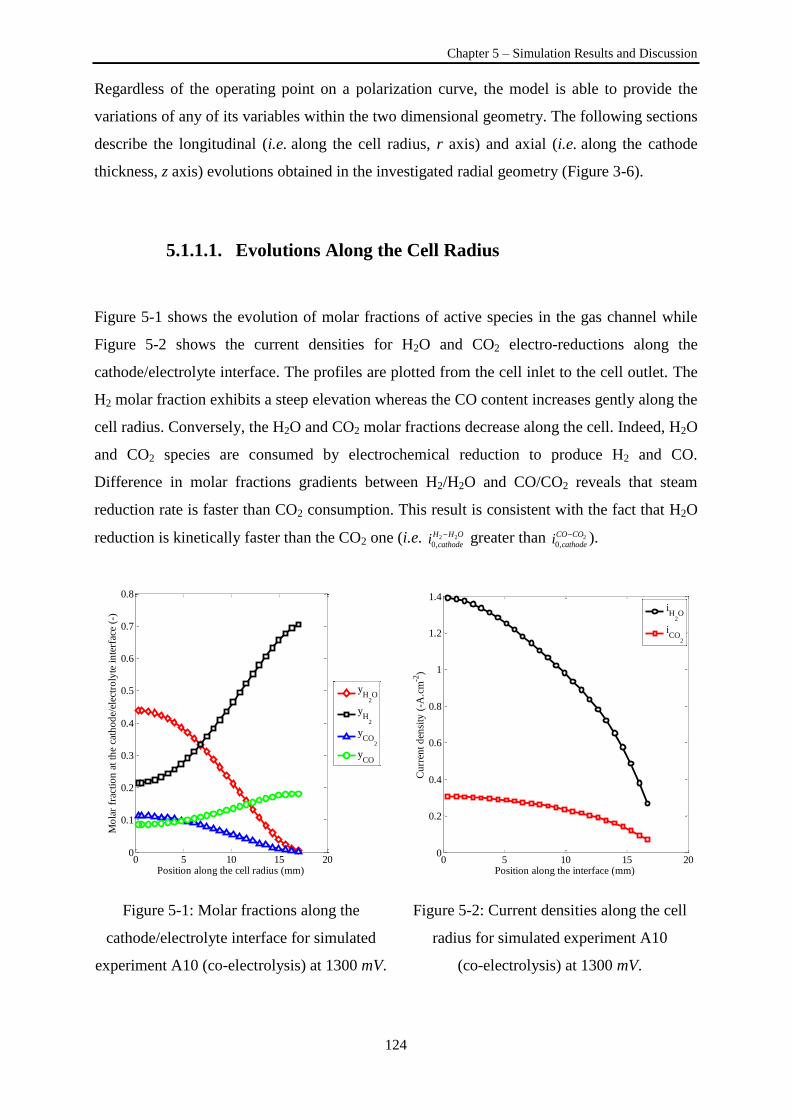
Chapter 5 – Simulation Results and Discussion
124
Regardless of the operating point on a polarization curve, the model is able to provide the
variations of any of its variables within the two dimensional geometry. The following sections
describe the longitudinal (i.e. along the cell radius, r axis) and axial (i.e. along the cathode
thickness, z axis) evolutions obtained in the investigated radial geometry (Figure 3-6).
5.1.1.1. Evolutions Along the Cell Radius
Figure 5-1 shows the evolution of molar fractions of active species in the gas channel while
Figure 5-2 shows the current densities for H2O and CO2 electro-reductions along the
cathode/electrolyte interface. The profiles are plotted from the cell inlet to the cell outlet. The
H2 molar fraction exhibits a steep elevation whereas the CO content increases gently along the
cell radius. Conversely, the H2O and CO2 molar fractions decrease along the cell. Indeed, H2O
and CO2 species are consumed by electrochemical reduction to produce H2 and CO.
Difference in molar fractions gradients between H2/H2O and CO/CO2 reveals that steam
reduction rate is faster than CO2 consumption. This result is consistent with the fact that H2O
reduction is kinetically faster than the CO2 one (i.e. 2 2
0,
H H O
cathodei greater than
2
0,
CO CO
cathodei ).
Figure 5-1: Molar fractions along the
cathode/electrolyte interface for simulated
experiment A10 (co-electrolysis) at 1300 mV.
Figure 5-2: Current densities along the cell
radius for simulated experiment A10
(co-electrolysis) at 1300 mV.
0 5 10 15 200
0.1
0.2
0.3
0.4
0.5
0.6
0.7
0.8
Position along the cell radius (mm)
Mo
lar
frac
tio
n a
t th
e ca
tho
de/
elec
tro
lyte
in
terf
ace
(-)
yH
2O
yH
2
yCO
2
yCO
0 5 10 15 200
0.2
0.4
0.6
0.8
1
1.2
1.4
Position along the interface (mm)
Cu
rren
t d
ensi
ty (
-A.c
m-2
)
iH
2O
iCO
2
Chapter 5 – Simulation Results and Discussion
125
As shown in Figure 5-2, local current densities decrease steeply from the cell center to the
cathode outlet. Indeed, H2O and CO2 are highly converted along the cell, yielding lower
amounts of reactants available at the electrode/electrolyte interface for reduction. This
supports the high global faradaic conversion rate of 99% computed.
It is worth noting that the average electrochemical production rate of H2 is here roughly three
times higher than that of CO at the cathode/electrolyte interface. This confirms that CO2
electrolysis can occur in parallel of H2O electrolysis, which is consistent with the CO/CO2
single electrolysis experimental feasibility, presented in Chapter 4.
Figure 5-3 illustrates the Nernst potential and the overpotentials related to steam electrolysis
in co-electrolysis operation, plotted along the cell radius. It can be noticed that the sum of all
the overpotentials to the Nernst potential is equal to the cell voltage of 1300 mV (Equation (3-
19)). This result highlights the reliability of overpotential calculations along the cell radius
(cf. section 3.2.6).
Ohmic and activation overpotentials are decreasing functions of the distance from the center
as they directly depend on the current density (cf. Equations (3-19) and (3-28)). In agreement
with the chosen values for anode and cathode exchange current densities
( 2 2/
0,
H H O
cathodei = 560 mA.cm-2
and 0,
LSM YSZ
anodei = 200 mA.cm
-2), it is found that the anode activation
overpotential is higher than cathode activation contribution.
It is also shown that the anodic concentration overpotential remains negligible regardless of
the position along the cell. This can be related to the thin anode that does not significantly
contribute to the mass transport limitation. Let us recall that even if the oxygen molar fraction
rises up to 2
int_ 0i
Oy = 1 atm, according to Equation (3-32) with
2
int_ 0i
Oy = 0.21 atm, the anode
concentration overpotential would only be equal to 36 mV. As the global steam conversion
rate is higher than 94%, the steam molar fraction falls close to zero at the cell outlet (Figure 5-
1). Accordingly, the cathode concentration overpotential increases strongly along the cell to
account for up to 77% of the total voltage at the outer cell boundary (Figure 5-3). It is worth
noting that very similar responses are predicted concerning CO2 reduction. However, the
ohmic overpotential is lower because of a low current density related to CO2 electrolysis
(Figure 5-2).
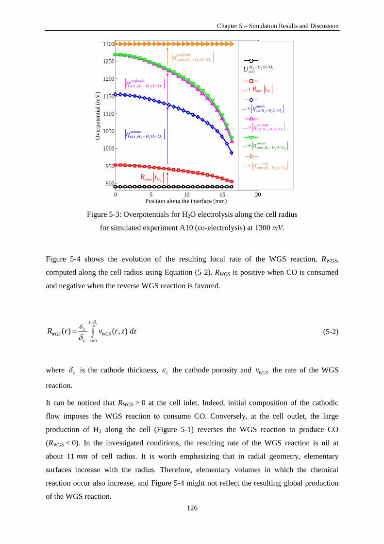
Chapter 5 – Simulation Results and Discussion
126
Figure 5-3: Overpotentials for H2O electrolysis along the cell radius
for simulated experiment A10 (co-electrolysis) at 1300 mV.
Figure 5-4 shows the evolution of the resulting local rate of the WGS reaction, RWGS,
computed along the cell radius using Equation (5-2). RWGS is positive when CO is consumed
and negative when the reverse WGS reaction is favored.
0
( ) ( , ) cz
cWGS WGS
c z
R r v r z dz
(5-2)
where c is the cathode thickness, c the cathode porosity and WGSv the rate of the WGS
reaction.
It can be noticed that RWGS > 0 at the cell inlet. Indeed, initial composition of the cathodic
flow imposes the WGS reaction to consume CO. Conversely, at the cell outlet, the large
production of H2 along the cell (Figure 5-1) reverses the WGS reaction to produce CO
(RWGS < 0). In the investigated conditions, the resulting rate of the WGS reaction is nil at
about 11 mm of cell radius. It is worth emphasizing that in radial geometry, elementary
surfaces increase with the radius. Therefore, elementary volumes in which the chemical
reaction occur also increase, and Figure 5-4 might not reflect the resulting global production
of the WGS reaction.
0 5 10 15 20
900
950
1000
1050
1100
1150
1200
1250
1300
Position along the interface (mm)
Ov
erp
ote
nti
al (
mV
)
2 2 2, / / ... cathode
conc H H O O
2 2 2, / / ... anode
conc H H O O
2 2 2, / / ... cathode
act H H O O
2 2 2, / / ... anode
act H H O O
2 ... ohm HR i
2 2 2/ /
0 H H O O
iU
2ohm HR i
2 2 2, / /
anode
act H H O O
2 2 2, / /
cathode
act H H O O
2 2 2, / /
cathode
conc H H O O
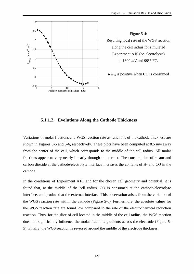
Chapter 5 – Simulation Results and Discussion
127
Figure 5-4:
Resulting local rate of the WGS reaction
along the cell radius for simulated
Experiment A10 (co-electrolysis)
at 1300 mV and 99% FC.
RWGS is positive when CO is consumed
5.1.1.2. Evolutions Along the Cathode Thickness
Variations of molar fractions and WGS reaction rate as functions of the cathode thickness are
shown in Figures 5-5 and 5-6, respectively. These plots have been computed at 8.5 mm away
from the center of the cell, which corresponds to the middle of the cell radius. All molar
fractions appear to vary nearly linearly through the cermet. The consumption of steam and
carbon dioxide at the cathode/electrolyte interface increases the contents of H2 and CO in the
cathode.
In the conditions of Experiment A10, and for the chosen cell geometry and potential, it is
found that, at the middle of the cell radius, CO is consumed at the cathode/electrolyte
interface, and produced at the external interface. This observation arises from the variation of
the WGS reaction rate within the cathode (Figure 5-6). Furthermore, the absolute values for
the WGS reaction rate are found low compared to the rate of the electrochemical reduction
reaction. Thus, for the slice of cell located in the middle of the cell radius, the WGS reaction
does not significantly influence the molar fractions gradients across the electrode (Figure 5-
5). Finally, the WGS reaction is reversed around the middle of the electrode thickness.
0 5 10 15 20-0.5
0
0.5
1
1.5
2
2.5
3
Position along the cell radius (mm)
RW
GS (
mo
l.s-1
.m-3
)
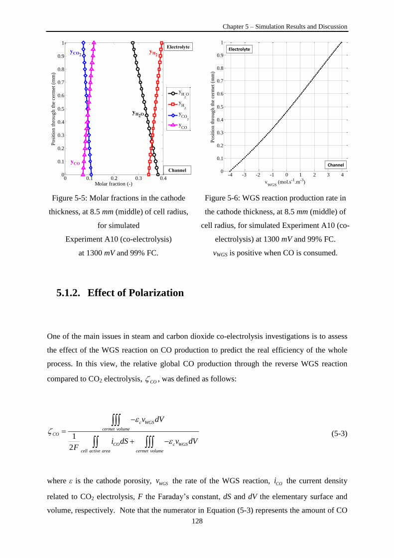
Chapter 5 – Simulation Results and Discussion
128
Figure 5-5: Molar fractions in the cathode
thickness, at 8.5 mm (middle) of cell radius,
for simulated
Experiment A10 (co-electrolysis)
at 1300 mV and 99% FC.
Figure 5-6: WGS reaction production rate in
the cathode thickness, at 8.5 mm (middle) of
cell radius, for simulated Experiment A10 (co-
electrolysis) at 1300 mV and 99% FC.
vWGS is positive when CO is consumed.
5.1.2. Effect of Polarization
One of the main issues in steam and carbon dioxide co-electrolysis investigations is to assess
the effect of the WGS reaction on CO production to predict the real efficiency of the whole
process. In this view, the relative global CO production through the reverse WGS reaction
compared to CO2 electrolysis, CO , was defined as follows:
1
2
c WGS
cermet volumeCO
CO c WGS
cell active area cermet volume
v dV
i dS v dVF
(5-3)
where ε is the cathode porosity, WGSv the rate of the WGS reaction, COi the current density
related to CO2 electrolysis, F the Faraday’s constant, dS and dV the elementary surface and
volume, respectively. Note that the numerator in Equation (5-3) represents the amount of CO
0 0.1 0.2 0.3 0.40
0.1
0.2
0.3
0.4
0.5
0.6
0.7
0.8
0.9
1
Molar fraction (-)
Po
siti
on
th
rou
gh
th
e ce
rmet
(m
m)
yH
2O
yH
2
yCO
2
yCO
Electrolyte
Channel
yH2O
yH2yCO2
yCO
-4 -3 -2 -1 0 1 2 3 40
0.1
0.2
0.3
0.4
0.5
0.6
0.7
0.8
0.9
1
Po
siti
on
th
rou
gh
th
e ce
rmet
(m
m)
vWGS
(mol.s-1
.m-3
)
Electrolyte
Channel
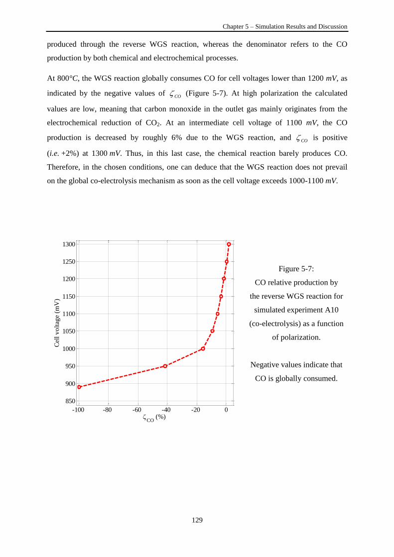
Chapter 5 – Simulation Results and Discussion
129
produced through the reverse WGS reaction, whereas the denominator refers to the CO
production by both chemical and electrochemical processes.
At 800°C, the WGS reaction globally consumes CO for cell voltages lower than 1200 mV, as
indicated by the negative values of CO (Figure 5-7). At high polarization the calculated
values are low, meaning that carbon monoxide in the outlet gas mainly originates from the
electrochemical reduction of CO2. At an intermediate cell voltage of 1100 mV, the CO
production is decreased by roughly 6% due to the WGS reaction, and CO is positive
(i.e. +2%) at 1300 mV. Thus, in this last case, the chemical reaction barely produces CO.
Therefore, in the chosen conditions, one can deduce that the WGS reaction does not prevail
on the global co-electrolysis mechanism as soon as the cell voltage exceeds 1000-1100 mV.
Figure 5-7:
CO relative production by
the reverse WGS reaction for
simulated experiment A10
(co-electrolysis) as a function
of polarization.
Negative values indicate that
CO is globally consumed.
-100 -80 -60 -40 -20 0
850
900
950
1000
1050
1100
1150
1200
1250
1300
CO
(%)
Cel
l v
olt
age
(mV
)
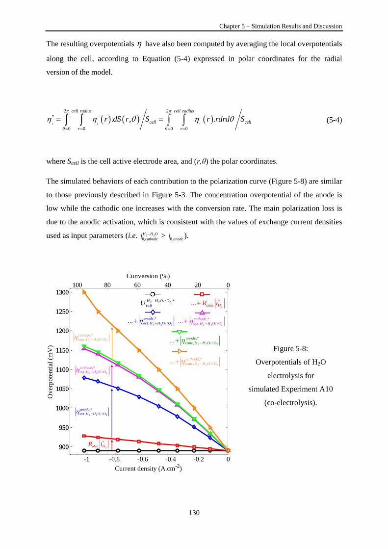
Chapter 5 – Simulation Results and Discussion
130
The resulting overpotentials have also been computed by averaging the local overpotentials
along the cell, according to Equation (5-4) expressed in polar coordinates for the radial
version of the model.
2 2
*
0 0 0 0
. , .i i i
cell radius cell radius
cell cell
r r
r dS r S r rdrd S
(5-4)
where Scell is the cell active electrode area, and (r,θ) the polar coordinates.
The simulated behaviors of each contribution to the polarization curve (Figure 5-8) are similar
to those previously described in Figure 5-3. The concentration overpotential of the anode is
low while the cathodic one increases with the conversion rate. The main polarization loss is
due to the anodic activation, which is consistent with the values of exchange current densities
used as input parameters (i.e. 2 2
0,
H H O
cathodei > 0,anodei ).
Figure 5-8:
Overpotentials of H2O
electrolysis for
simulated Experiment A10
(co-electrolysis).
-1 -0.8 -0.6 -0.4 -0.2 0
900
950
1000
1050
1100
1150
1200
1250
1300
Current density (A.cm-2
)
Ov
erp
ote
nti
al (
mV
)
020406080100
900
950
1000
1050
1100
1150
1200
1250
1300
Conversion (%)
2 2 2
,*
, / / ... cathode
conc H H O O
2 2 2
,*
, / / ... anode
conc H H O O
2 2 2
,*
, / / ... cathode
act H H O O 2 2 2
,*
, / / ... anode
act H H O O
2
* ... ohm HR i2 2 2/ / ,*
0 H H O O
iU
2
*
ohm HR i
2 2 2
,*
, / /
anode
act H H O O
2 2 2
,*
, / /
cathode
act H H O O
2 2 2
,*
, / /
cathode
conc H H O O
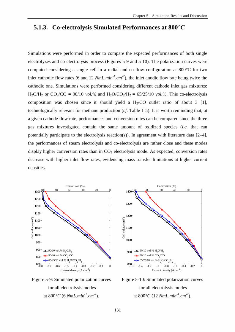
Chapter 5 – Simulation Results and Discussion
131
5.1.3. Co-electrolysis Simulated Performances at 800°C
Simulations were performed in order to compare the expected performances of both single
electrolyzes and co-electrolysis process (Figures 5-9 and 5-10). The polarization curves were
computed considering a single cell in a radial and co-flow configuration at 800°C for two
inlet cathodic flow rates (6 and 12 NmL.min-1
.cm-2
), the inlet anodic flow rate being twice the
cathodic one. Simulations were performed considering different cathode inlet gas mixtures:
H2O/H2 or CO2/CO = 90/10 vol.% and H2O/CO2/H2 = 65/25/10 vol.%. This co-electrolysis
composition was chosen since it should yield a H2/CO outlet ratio of about 3 [1],
technologically relevant for methane production (cf. Table 1-5). It is worth reminding that, at
a given cathode flow rate, performances and conversion rates can be compared since the three
gas mixtures investigated contain the same amount of oxidized species (i.e. that can
potentially participate to the electrolysis reaction(s)). In agreement with literature data [2–4],
the performances of steam electrolysis and co-electrolysis are rather close and these modes
display higher conversion rates than in CO2 electrolysis mode. As expected, conversion rates
decrease with higher inlet flow rates, evidencing mass transfer limitations at higher current
densities.
Figure 5-9: Simulated polarization curves
for all electrolysis modes
at 800°C (6 NmL.min-1
.cm-2
).
Figure 5-10: Simulated polarization curves
for all electrolysis modes
at 800°C (12 NmL.min-1
.cm-2
).
-0.8 -0.7 -0.6 -0.5 -0.4 -0.3 -0.2 -0.1 0800
850
900
950
1000
1050
1100
1150
1200
1250
1300
Current density (A.cm-2
)
Cel
l v
olt
age
(mV
)
90/10 vol.% H2O/H
2
90/10 vol.% CO2/CO
65/25/10 vol.% H2O/CO
2/H
2
020406080100
800
850
900
950
1000
1050
1100
1150
1200
1250
1300
Conversion (%)
-1.6 -1.4 -1.2 -1 -0.8 -0.6 -0.4 -0.2 0800
900
1000
1100
1200
1300
1400
Current density (A.cm-2
)
Cel
l v
olt
age
(mV
)
90/10 vol.% H2O/H
2
90/10 vol.% CO2/CO
65/25/10 vol.% H2O/CO
2/H
2
020406080100
800
900
1000
1100
1200
1300
1400
Conversion (%)
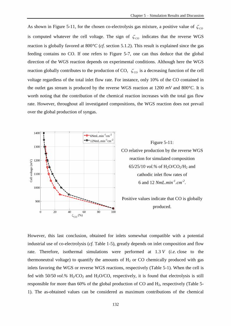
Chapter 5 – Simulation Results and Discussion
132
As shown in Figure 5-11, for the chosen co-electrolysis gas mixture, a positive value of CO
is computed whatever the cell voltage. The sign of CO indicates that the reverse WGS
reaction is globally favored at 800°C (cf. section 5.1.2). This result is explained since the gas
feeding contains no CO. If one refers to Figure 5-7, one can thus deduce that the global
direction of the WGS reaction depends on experimental conditions. Although here the WGS
reaction globally contributes to the production of CO, CO is a decreasing function of the cell
voltage regardless of the total inlet flow rate. For instance, only 10% of the CO contained in
the outlet gas stream is produced by the reverse WGS reaction at 1200 mV and 800°C. It is
worth noting that the contribution of the chemical reaction increases with the total gas flow
rate. However, throughout all investigated compositions, the WGS reaction does not prevail
over the global production of syngas.
Figure 5-11:
CO relative production by the reverse WGS
reaction for simulated composition
65/25/10 vol.% of H2O/CO2/H2 and
cathodic inlet flow rates of
6 and 12 NmL.min-1
.cm-2
.
Positive values indicate that CO is globally
produced.
However, this last conclusion, obtained for inlets somewhat compatible with a potential
industrial use of co-electrolysis (cf. Table 1-5), greatly depends on inlet composition and flow
rate. Therefore, isothermal simulations were performed at 1.3 V (i.e. close to the
thermoneutral voltage) to quantify the amounts of H2 or CO chemically produced with gas
inlets favoring the WGS or reverse WGS reactions, respectively (Table 5-1). When the cell is
fed with 50/50 vol.% H2/CO2 and H2O/CO, respectively, it is found that electrolysis is still
responsible for more than 60% of the global production of CO and H2, respectively (Table 5-
1). The as-obtained values can be considered as maximum contributions of the chemical
0 20 40 60 80 100
900
1000
1100
1200
1300
1400
CO
(%)
Cel
l v
olt
age
(mV
)
6NmL.min-1
cm-2
12NmL.min-1
cm-2
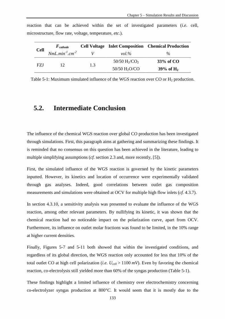
Chapter 5 – Simulation Results and Discussion
133
reaction that can be achieved within the set of investigated parameters (i.e. cell,
microstructure, flow rate, voltage, temperature, etc.).
Cell Fcathode Cell Voltage Inlet Composition Chemical Production
NmL.min-1
.cm-2
V vol.% %
FZJ 12 1.3 50/50 H2/CO2 33% of CO
50/50 H2O/CO 39% of H2
Table 5-1: Maximum simulated influence of the WGS reaction over CO or H2 production.
5.2. Intermediate Conclusion
The influence of the chemical WGS reaction over global CO production has been investigated
through simulations. First, this paragraph aims at gathering and summarizing these findings. It
is reminded that no consensus on this question has been achieved in the literature, leading to
multiple simplifying assumptions (cf. section 2.3 and, more recently, [5]).
First, the simulated influence of the WGS reaction is governed by the kinetic parameters
inputted. However, its kinetics and location of occurrence were experimentally validated
through gas analyses. Indeed, good correlations between outlet gas composition
measurements and simulations were obtained at OCV for multiple high flow inlets (cf. 4.3.7).
In section 4.3.10, a sensitivity analysis was presented to evaluate the influence of the WGS
reaction, among other relevant parameters. By nullifying its kinetic, it was shown that the
chemical reaction had no noticeable impact on the polarization curve, apart from OCV.
Furthermore, its influence on outlet molar fractions was found to be limited, in the 10% range
at higher current densities.
Finally, Figures 5-7 and 5-11 both showed that within the investigated conditions, and
regardless of its global direction, the WGS reaction only accounted for less that 10% of the
total outlet CO at high cell polarization (i.e. Ucell > 1100 mV). Even by favoring the chemical
reaction, co-electrolysis still yielded more than 60% of the syngas production (Table 5-1).
These findings highlight a limited influence of chemistry over electrochemistry concerning
co-electrolyzer syngas production at 800°C. It would seem that it is mostly due to the
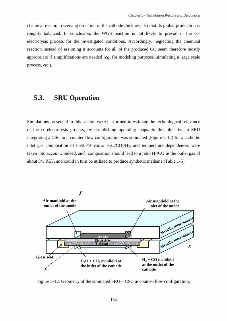
Chapter 5 – Simulation Results and Discussion
134
chemical reaction reversing direction in the cathode thickness, so that its global production is
roughly balanced. In conclusion, the WGS reaction is not likely to prevail in the co-
electrolysis process for the investigated conditions. Accordingly, neglecting the chemical
reaction instead of assuming it accounts for all of the produced CO seem therefore mostly
appropriate if simplifications are needed (eg. for modeling purposes, simulating a large scale
process, etc.).
5.3. SRU Operation
Simulations presented in this section were performed to estimate the technological relevance
of the co-electrolysis process, by establishing operating maps. In this objective, a SRU
integrating a CSC in a counter-flow configuration was simulated (Figure 5-12) for a cathodic
inlet gas composition of 65/25/10 vol.% H2O/CO2/H2, and temperature dependences were
taken into account. Indeed, such composition should lead to a ratio H2/CO in the outlet gas of
about 3/1 REF, and could in turn be utilized to produce synthetic methane (Table 1-5).
Figure 5-12: Geometry of the simulated SRU – CSC in counter-flow configuration.
Air manifold at the
outlet of anode
Air manifold at the
inlet of anode
H2 manifold at the
outlet of cathodeSteam manifold at
the inlet of cathode
Metallic in
terconnect
Metallic in
terconnect
x
y
z
Glass seal
Air manifold at the
outlet of anode
Air manifold at the
inlet of anode
H2 manifold at the
outlet of cathodeSteam manifold at
the inlet of cathode
Metallic in
terconnect
Metallic in
terconnect
x
y
z
Glass sealH2O + CO2 manifold at
the intlet of the cathode
H2 + CO manifold
at the outlet of the
cathode
Air manifold at the
outlet of the anodeAir manifold at the
inlet of the anode
Cathode
Chapter 5 – Simulation Results and Discussion
135
5.3.1. Simulation Parameters
The influence of the temperature on co-electrolysis polarization curve was investigated at the
SRU level based on the classical geometry of Figure 5-12 [6] (planar CSC in counter-flow
feeding), integrating a 10×10 cm2 FZJ cell, and by coupling the electrochemical and thermal
modules (cf. 3.2.5). According to the results obtained for a radial configuration is isothermal
conditions, the previous sections, the composition of the cathode inlet gas stream was
65/25/10 vol.% H2O/CO2/H2, while the anode was fed with air (Table 5-2). A wide range of
flow rates, and thus conversion rates, was examined, from 12 to 48 NmL.min-1
.cm-2
.
The influence of temperature on exchange current densities was taken into account through
corresponding activation energies (Table 5-2), according to an Arrhenius type behavior:
0
0 0 exp aEi T i
RT
(5-5)
where 0i is the exchange current density, 0
0i the pre-exponential factor and aE the activation
energy.
Pre-exponential factors were tuned to obtain 530, 356 and 200 mA.cm-2
for 2 2
0,
H H O
cathodei
, 2
0,
CO CO
cathodei
and 0,anodei , respectively, at 800°C. All remaining numerical values concerning the thermal
description can be found in references [6–8].
The following sections highlight some of the results obtained with simulated conditions C2
(Table 5-2), before presenting the computed operating maps for co-electrolysis operation.
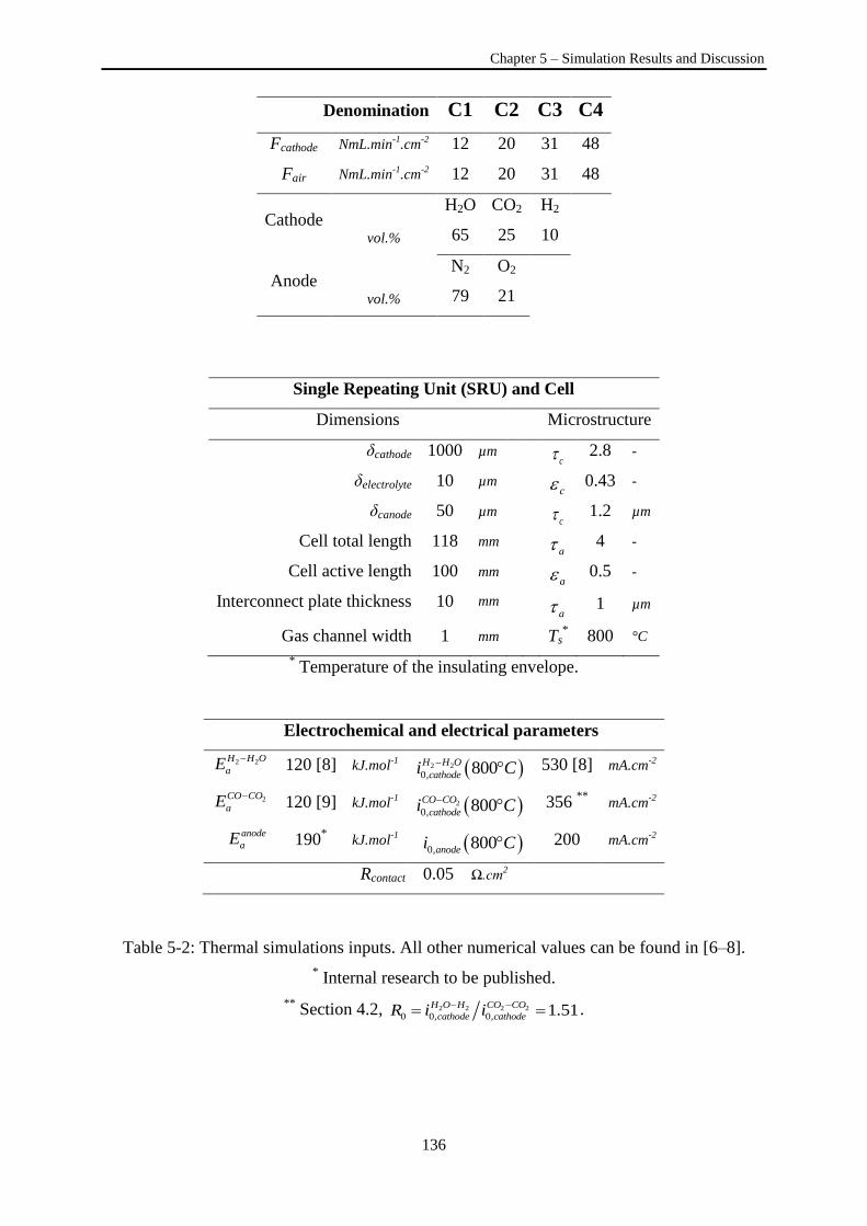
Chapter 5 – Simulation Results and Discussion
136
Single Repeating Unit (SRU) and Cell
Dimensions Microstructure
δcathode 1000 µm c
2.8 -
δelectrolyte 10 µm c
0.43 -
δcanode 50 µm c
1.2 µm
Cell total length 118 mm a
4 -
Cell active length 100 mm a
0.5 -
Interconnect plate thickness 10 mm a
1 µm
Gas channel width 1 mm Ts* 800 °C
* Temperature of the insulating envelope.
Electrochemical and electrical parameters
2 2H H O
aE 120 [8] kJ.mol
-1 2 2
0, 800H H O
cathodei C
530 [8] mA.cm-2
2CO CO
aE 120 [9] kJ.mol-1
2
0, 800CO CO
cathodei C
356 **
mA.cm-2
anode
aE 190* kJ.mol
-1 0, 800anodei C
200 mA.cm-2
Rcontact 0.05 Ω.cm2
Table 5-2: Thermal simulations inputs. All other numerical values can be found in [6–8].
* Internal research to be published.
** Section 4.2, 2 2 2 2
0 0, 0, 1.51H O H CO CO
cathode cathodeR i i .
Denomination C1 C2 C3 C4
Fcathode NmL.min-1
.cm-2
12 20 31 48
Fair NmL.min-1
.cm-2
12 20 31 48
Cathode vol.%
H2O CO2 H2
65 25 10
Anode vol.%
N2 O2
79 21
Chapter 5 – Simulation Results and Discussion
137
5.3.2. Polarization Curve at 20 NmL.min-1
.cm-2
The effect of temperature on the polarization curve of the simulated SRU operating in
conditions C2 (Table 5-2) is shown in Figure 5-13.
At OCV, the cell temperature is about 797.5°C (i.e. 3°C less than the temperature of the
insulating envelope as described in Chapter 3). Indeed, the inlet cathodic composition
corresponds roughly to the thermodynamic equilibrium of the WGS reaction at 800°C. Thus,
the thermal sources related to the chemical reaction have a barely noticeable impact on both
cell temperature and gases composition along the cell at OCV. A more significant influence
can be anticipated by changing the inlet composition.
Figure 5-13A compares the polarization curves of the SRU obtained with the complete model
(i.e. taking into account the thermal module) and in isothermal conditions, respectively. It also
reports the temperature taken at the middle of the cell length (Figure 5-13B). It can be noted
that because of CO2 parallel electrolysis and WGS reaction, the thermoneutral voltage is
shifted compared to single steam electrolysis. This phenomenon has been experimentally
observed by following cell temperature slight changes during co-electrolysis i-V curves
recording. In the simulated conditions considered, the thermoneutral voltage is assessed at
about 1.32 V. As expected [1], the co-electrolysis thermoneutral voltage is comprised between
those of steam electrolysis (1.29 V) and CO2 electrolysis (1.46 V).
Similarly to observations in single steam electrolysis [6] (cf. Figure 1-9), the three operating
thermal modes can be detected. For cell voltages bellow the thermoneutral voltage, the
endothermicity of electrolysis reactions is not balanced by heat sources and thus, the cell
temperature drops below the one at OCV. Accordingly, the current density is lower than in
isothermal operation since local temperatures influence the ionic conductivity of the
electrolyte, the chemical and electrochemical kinetics, etc. Conversely, above the
thermoneutral voltage (i.e. exothermic operation), cell performances are enhanced. For
example, at 1400 mV, the cell current density rises from -1.62 to -2.09 A.cm-2
when the
exothermicity is taken into account. Furthermore, the distribution of thermal fluxes reveals
that about 75% of the produced heat is dissipated through radiative flow along this
polarization curve. Conversely, the remaining 25% is evacuated through gas convection.
These values are consistent with the ones reported on a CSC in steam electrolysis mode [6].
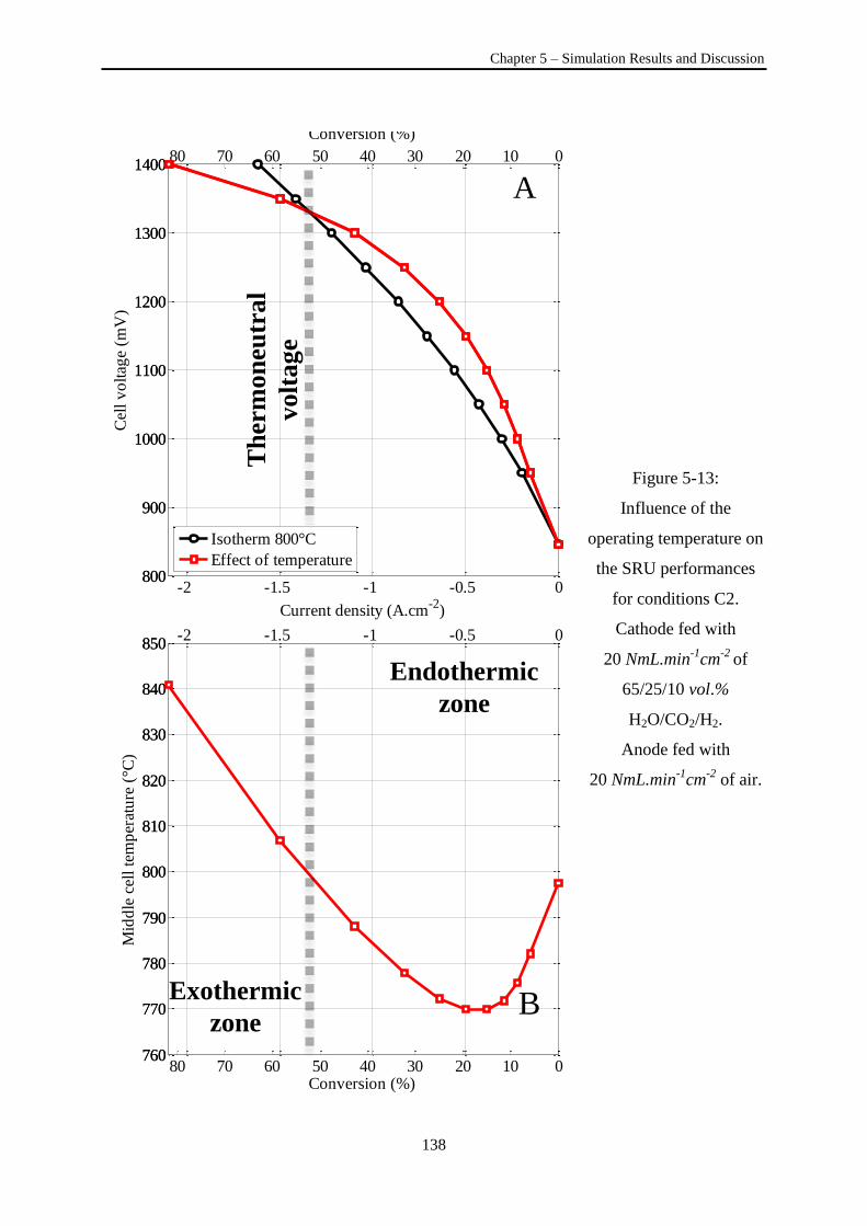
Chapter 5 – Simulation Results and Discussion
138
Figure 5-13:
Influence of the
operating temperature on
the SRU performances
for conditions C2.
Cathode fed with
20 NmL.min-1
cm-2
of
65/25/10 vol.%
H2O/CO2/H2.
Anode fed with
20 NmL.min-1
cm-2
of air.
-2 -1.5 -1 -0.5 0
760
770
780
790
800
810
820
830
840
850
Mid
dle
cel
l te
mp
erat
ure
(°C
)
01020304050607080760
770
780
790
800
810
820
830
840
850
Conversion (%)
-2 -1.5 -1 -0.5 0800
900
1000
1100
1200
1300
1400
Current density (A.cm-2
)
Cel
l v
olt
age
(mV
)
Isotherm 800°C
Effect of temperature
01020304050607080
800
900
1000
1100
1200
1300
1400
Conversion (%)
Endothermic
zone
Exothermic
zone
Th
erm
on
eu
tra
l
vo
lta
ge
A
B
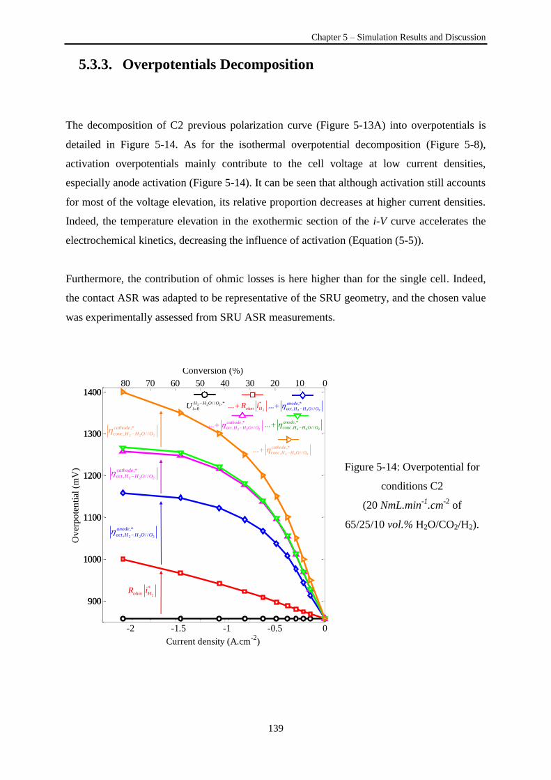
Chapter 5 – Simulation Results and Discussion
139
5.3.3. Overpotentials Decomposition
The decomposition of C2 previous polarization curve (Figure 5-13A) into overpotentials is
detailed in Figure 5-14. As for the isothermal overpotential decomposition (Figure 5-8),
activation overpotentials mainly contribute to the cell voltage at low current densities,
especially anode activation (Figure 5-14). It can be seen that although activation still accounts
for most of the voltage elevation, its relative proportion decreases at higher current densities.
Indeed, the temperature elevation in the exothermic section of the i-V curve accelerates the
electrochemical kinetics, decreasing the influence of activation (Equation (5-5)).
Furthermore, the contribution of ohmic losses is here higher than for the single cell. Indeed,
the contact ASR was adapted to be representative of the SRU geometry, and the chosen value
was experimentally assessed from SRU ASR measurements.
Figure 5-14: Overpotential for
conditions C2
(20 NmL.min-1
.cm-2
of
65/25/10 vol.% H2O/CO2/H2).
-2 -1.5 -1 -0.5 0
900
1000
1100
1200
1300
1400
Current density (A.cm-2
)
Ov
erp
ote
nti
al (
mV
)
01020304050607080
900
1000
1100
1200
1300
1400
Conversion (%)
2 2 2
,*
, / /... cathode
conc H H O O
2 2 2
,*
, / /... anode
conc H H O O 2 2 2
,*
, / /... cathode
act H H O O
2 2 2
,*
, / /... anode
act H H O O 2
*... ohm HR i2 2 2/ / ,*
0
H H O O
iU
2
*
ohm HR i
2 2 2
,*
, / /
anode
act H H O O
2 2 2
,*
, / /
cathode
act H H O O
2 2 2
,*
, / /
cathode
conc H H O O
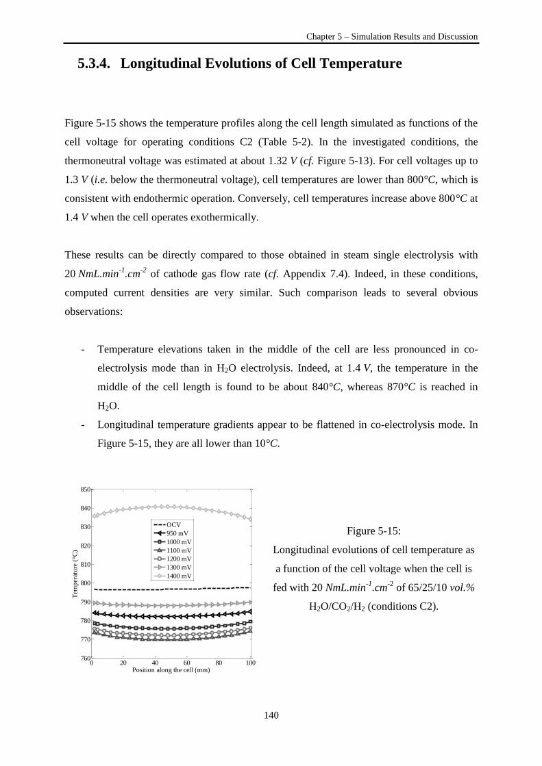
Chapter 5 – Simulation Results and Discussion
140
5.3.4. Longitudinal Evolutions of Cell Temperature
Figure 5-15 shows the temperature profiles along the cell length simulated as functions of the
cell voltage for operating conditions C2 (Table 5-2). In the investigated conditions, the
thermoneutral voltage was estimated at about 1.32 V (cf. Figure 5-13). For cell voltages up to
1.3 V (i.e. below the thermoneutral voltage), cell temperatures are lower than 800°C, which is
consistent with endothermic operation. Conversely, cell temperatures increase above 800°C at
1.4 V when the cell operates exothermically.
These results can be directly compared to those obtained in steam single electrolysis with
20 NmL.min-1
.cm-2
of cathode gas flow rate (cf. Appendix 7.4). Indeed, in these conditions,
computed current densities are very similar. Such comparison leads to several obvious
observations:
- Temperature elevations taken in the middle of the cell are less pronounced in co-
electrolysis mode than in H2O electrolysis. Indeed, at 1.4 V, the temperature in the
middle of the cell length is found to be about 840°C, whereas 870°C is reached in
H2O.
- Longitudinal temperature gradients appear to be flattened in co-electrolysis mode. In
Figure 5-15, they are all lower than 10°C.
Figure 5-15:
Longitudinal evolutions of cell temperature as
a function of the cell voltage when the cell is
fed with 20 NmL.min-1
.cm-2
of 65/25/10 vol.%
H2O/CO2/H2 (conditions C2).
0 20 40 60 80 100760
770
780
790
800
810
820
830
840
850
Position along the cell (mm)
Tem
per
atu
re (
°C)
OCV
950 mV
1000 mV
1100 mV
1200 mV
1300 mV
1400 mV
Chapter 5 – Simulation Results and Discussion
141
The differences in cell temperatures and thermal profiles between co-electrolysis and H2O
electrolysis modes could be explained by several factors. First, the volumetric heat capacity of
the cathode gas mixture is increased in co-electrolysis operation. Indeed, both CO and CO2
display greater Cp (33.7 and 55.4 J.mol-1
.K-1
respectively) than H2 and H2O (30.3 and
42.4 J.mol-1
.K-1
), respectively. Thus, cathode gas flows are able to evacuate more heat in co-
electrolysis than in H2O electrolysis. Also, the reverse WGS reaction, which is favored in the
chosen conditions, is slightly endothermic. Therefore, it alleviates the temperature increase
when the cell operates exothermically.
Besides the obvious advantage of co-electrolysis that is syngas generation, this simulated
SOC operating mode suggests an easier thermal management, especially crucial in stack
environment. Co-electrolysis could thus exhibit a wider range of acceptable operating
conditions compared to H2O electrolysis, since high thermal gradient have been shown to
cause mechanical stress, potentially leading to cell failure [10].
5.3.5. Longitudinal Evolutions of molar fractions and β
The profiles of molar fractions along the cathode/electrolyte interface, obtained with C2
inputs (Table 5-2) at 1.4 V, are shown in Figure 5-17. As they are being consumed, H2O and
CO2 molar fractions decrease along the cell, while those of H2 and CO increase, as expected.
In comparison with a radial geometry (Figure 5-1), molar fractions follow here a quasi linear
evolution. This arises from the longitudinal geometry in which every elementary cell active
areas are equivalent, whereas in radial geometries, elementary surfaces are a function of the
cell radius. However, the influence of conversion rates (i.e. higher concentration
overpotentials) can be seen here toward the cell outlet, where the consumption rates of
oxidized species are slower (i.e. the molar fraction evolutions digress from linear behaviors).
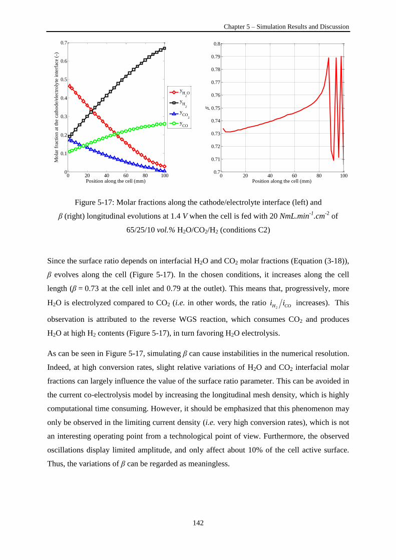
Chapter 5 – Simulation Results and Discussion
142
Figure 5-17: Molar fractions along the cathode/electrolyte interface (left) and
β (right) longitudinal evolutions at 1.4 V when the cell is fed with 20 NmL.min-1
.cm-2
of
65/25/10 vol.% H2O/CO2/H2 (conditions C2)
Since the surface ratio depends on interfacial H2O and CO2 molar fractions (Equation (3-18)),
β evolves along the cell (Figure 5-17). In the chosen conditions, it increases along the cell
length (β = 0.73 at the cell inlet and 0.79 at the outlet). This means that, progressively, more
H2O is electrolyzed compared to CO2 (i.e. in other words, the ratio 2H COi i increases). This
observation is attributed to the reverse WGS reaction, which consumes CO2 and produces
H2O at high H2 contents (Figure 5-17), in turn favoring H2O electrolysis.
As can be seen in Figure 5-17, simulating β can cause instabilities in the numerical resolution.
Indeed, at high conversion rates, slight relative variations of H2O and CO2 interfacial molar
fractions can largely influence the value of the surface ratio parameter. This can be avoided in
the current co-electrolysis model by increasing the longitudinal mesh density, which is highly
computational time consuming. However, it should be emphasized that this phenomenon may
only be observed in the limiting current density (i.e. very high conversion rates), which is not
an interesting operating point from a technological point of view. Furthermore, the observed
oscillations display limited amplitude, and only affect about 10% of the cell active surface.
Thus, the variations of β can be regarded as meaningless.
0 20 40 60 80 1000
0.1
0.2
0.3
0.4
0.5
0.6
0.7
Position along the cell (mm)
Mo
lar
frac
tio
n a
t th
e ca
tho
de/
elec
tro
lyte
in
terf
ace
(-)
yH
2O
yH
2
yCO
2
yCO
0 20 40 60 80 1000.7
0.71
0.72
0.73
0.74
0.75
0.76
0.77
0.78
0.79
0.8
Position along the cell (mm)

Chapter 5 – Simulation Results and Discussion
143
5.3.6. Co-electrolysis Operating Maps
This section presents the complete set of simulations detailed in Table 5-2. These operating
maps present the main parameters that characterize the co-electrolysis process, and should as
such be helpful to determine relevant conditions for co-electrolysis operation. In this view,
maps of current densities (Figure 5-18A) and conversion rates (Figure 5-18B) were plotted as
a function of cell voltage and inlet cathode gas flow rates. Note that these inlets correspond to
a mixture of 65/25/10 vol.% H2O/CO2/H2, while the anode is swept with the same flow rate of
air (Table 5-2). Additional relevant maps are given in Figures 5-19, 5-20 and 5-21.
At a given cell voltage, increasing the cathodic flux yields higher current densities due to
lower concentration overpotentials (Figure 5-18A), which can be attributed to lower
conversion rates, as shown in Figure 5-18B. Because the WGS reaction is conservative of
oxidized and reduced species, H2+CO production profiles follow those of current densities
(Figure 5-19A). The ratio of H2+CO production to electrical power is plotted in Figure 5-19B.
It is a combination of Figures 5-18A and 5-19A. It can be seen that this ratio increases with
lower cell voltages. Global heat source terms (Figure 5-20A) and resulting cell temperatures
(Figure 5-20B) are slightly dependent of inlet fluxes. Very similar observations can be made
concerning single H2O electrolysis operating maps, presented in Appendix 7.4. These last
maps were computed in similar conditions (same SRU geometry and cathode inlets composed
of 90/10 vol.% H2O/H2) [10].
Comparing H2O and co-electrolysis operating maps highlights several striking differences.
First, a maximum current density of about -2.2 A.cm-2
is obtained in co-electrolysis, whereas
about -6 A.cm-2
was calculated in steam electrolysis (Appendix 7.4). Such difference in
current density is mainly explained by a higher SRU temperature elevation in H2O
electrolysis. This stem from mass transport limitations due to CO and CO2 in the thick porous
cathode, and could be an overall limitation of the co-electrolysis process. However, such
lower current densities have positive repercussions on the SRU thermal management. Indeed,
the maximum temperature elevation obtained in co-electrolysis is limited to +40°C compared
to 800°C, which is significantly lower than for H2O electrolysis (Appendix 7.4). Furthermore,
in comparable conditions, temperature elevations are lowered in co-electrolysis than in H2O
electrolysis, so that this parameter does not appear here to be limiting.
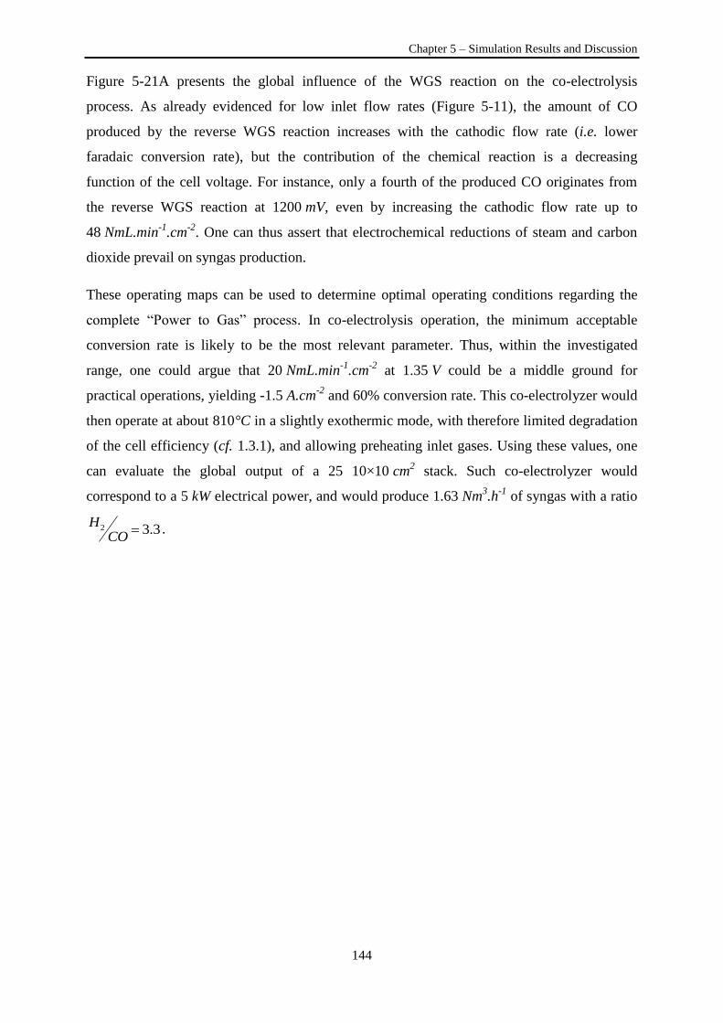
Chapter 5 – Simulation Results and Discussion
144
Figure 5-21A presents the global influence of the WGS reaction on the co-electrolysis
process. As already evidenced for low inlet flow rates (Figure 5-11), the amount of CO
produced by the reverse WGS reaction increases with the cathodic flow rate (i.e. lower
faradaic conversion rate), but the contribution of the chemical reaction is a decreasing
function of the cell voltage. For instance, only a fourth of the produced CO originates from
the reverse WGS reaction at 1200 mV, even by increasing the cathodic flow rate up to
48 NmL.min-1
.cm-2
. One can thus assert that electrochemical reductions of steam and carbon
dioxide prevail on syngas production.
These operating maps can be used to determine optimal operating conditions regarding the
complete “Power to Gas” process. In co-electrolysis operation, the minimum acceptable
conversion rate is likely to be the most relevant parameter. Thus, within the investigated
range, one could argue that 20 NmL.min-1
.cm-2
at 1.35 V could be a middle ground for
practical operations, yielding -1.5 A.cm-2
and 60% conversion rate. This co-electrolyzer would
then operate at about 810°C in a slightly exothermic mode, with therefore limited degradation
of the cell efficiency (cf. 1.3.1), and allowing preheating inlet gases. Using these values, one
can evaluate the global output of a 25 10×10 cm2 stack. Such co-electrolyzer would
correspond to a 5 kW electrical power, and would produce 1.63 Nm3.h
-1 of syngas with a ratio
2 3.3H
CO .

Chapter 5 – Simulation Results and Discussion
145
Figure 5-18: Co-electrolysis operating maps (1/4): Current densities (A-left)
and corresponding Faradaic conversion rates (B-right).
Figure 5-19: Co-electrolysis operating maps (2/4): Production of H2 and CO (A-left)
and Efficiency defined as the ratio of production over electrical power required (B-right).
15 20 25 30 35 40 45950
1000
1050
1100
1150
1200
1250
1300
1350
1400
0.150.15
0.30.3
0.3
0.450.45
0.45
0.60.6
0.6
0.750.75
0.75
0.90.9
0.9
1.051.05
1.05
1.21.2 1.2
1.351.35 1.35
1.51.5 1.5
1.651.65 1.65
1.81.8 1.8
1.951.95 1.95
2.1
2.1 2.1
2.25 2.25
Cathodic flux (NmL.min-1
.cm-2
)
Cel
l v
olt
age
(mV
)
Current density (-A.cm-2
)
15 20 25 30 35 40 45950
1000
1050
1100
1150
1200
1250
1300
1350
1400
5
5
5
10
10
10
10
15
15
15
15
20
20
20
20
25
25
25
25
30
30
30
30
35
35
35
35
40
40
40
40
45
45
45
50
50
50
55
55
60
60
65
65
70
70
7580
85
90
Cathodic flux (NmL.min-1
.cm-2
)
Cel
l v
olt
age
(mV
)
Conversion rate (%)
15 20 25 30 35 40 45950
1000
1050
1100
1150
1200
1250
1300
1350
1400
0.1
0.1
0.1
0.2
0.2
0.2
0.30.3
0.3
0.4
0.40.4
0.50.5
0.5
0.60.6
0.6
0.70.7 0.7
0.80.8 0.8
0.9
0.9 0.9
1 1
Cathodic flux (NmL.min-1
.cm-2
)
Cel
l v
olt
age
(mV
)
H2 + CO production (NL.h
-1.cm
-2)
15 20 25 30 35 40 45950
1000
1050
1100
1150
1200
1250
1300
1350
1400
1.921.951.98
1.982.01
2.01
2.04
2.042.04
2.07
2.072.07
2.12.1
2.12.13 2.13
2.132.16
2.16
2.16
2.19
2.192.19
2.2
2
2.22 2.22
2.22
2.2
5
2.25
2.252.25
2.2
8
2.28
2.282.28
2.3
1
2.31
2.31
2.31
2.3
4
2.34
2.34
2.37
2.37
2.37
2.4
2.4
2.4
2.43
2.43
2.46
2.46
2.49
2.49
2.52
2.55
Cathodic flux (NmL.min-1
.cm-2
)
Cel
l v
olt
age
(mV
)
Electrical power / Production (W.h.NL-1
)
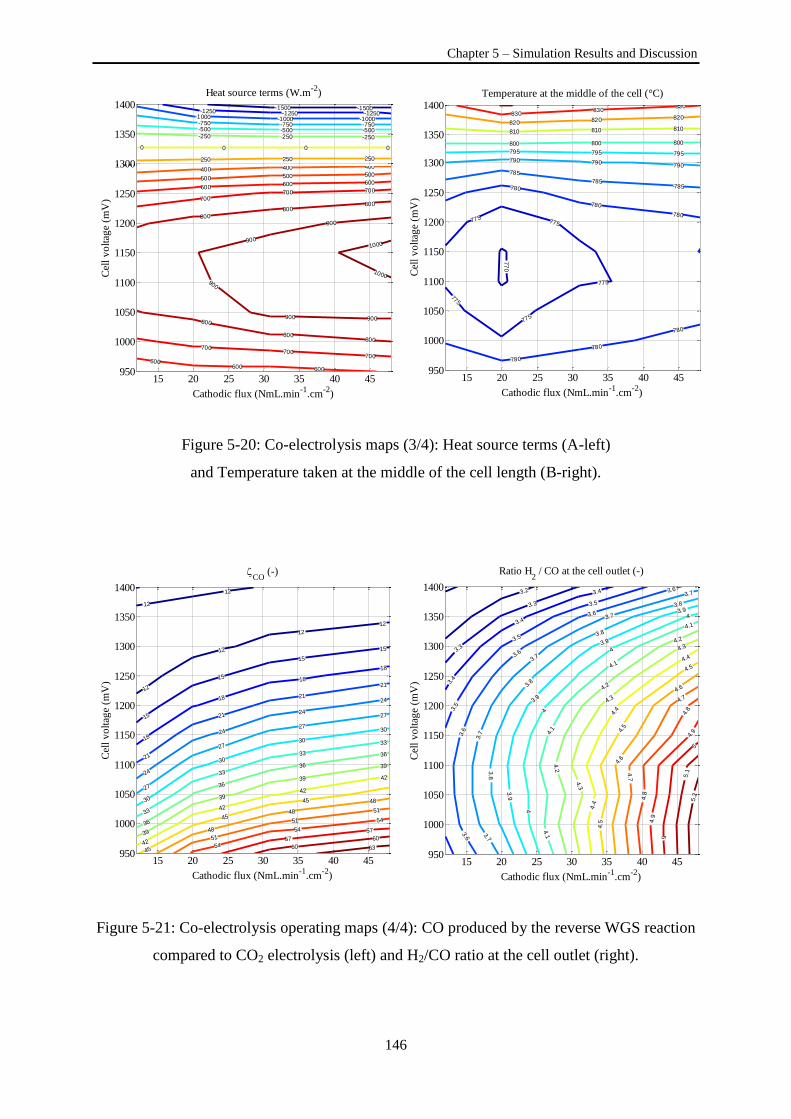
Chapter 5 – Simulation Results and Discussion
146
Figure 5-20: Co-electrolysis maps (3/4): Heat source terms (A-left)
and Temperature taken at the middle of the cell length (B-right).
Figure 5-21: Co-electrolysis operating maps (4/4): CO produced by the reverse WGS reaction
compared to CO2 electrolysis (left) and H2/CO ratio at the cell outlet (right).
15 20 25 30 35 40 45950
1000
1050
1100
1150
1200
1250
1300
1350
1400 -1600 -1600-1500 -1500-1400-1400 -1400-1300 -1300 -1300-1200 -1200 -1200-1100 -1100 -1100-1000 -1000 -1000-900 -900 -900-800 -800 -800-700 -700 -700-600 -600 -600-500 -500 -500-400 -400 -400-300 -300 -300
-200 -200 -200-100 -100 -100
0 0 0 0100 100 100200 200 200300 300 300
400 400 400
500 500 500
600600600
600600 600
700700 700
700700
700
800800
800
800
800800
900
900
900
900 900
1000
1000
Cathodic flux (NmL.min-1
.cm-2
)
Cel
l v
olt
age
(mV
)Heat source terms (W.m
-2)
15 20 25 30 35 40 45950
1000
1050
1100
1150
1200
1250
1300
1350
1400 -1500 -1500-1250 -1250 -1250-1000 -1000 -1000-750 -750 -750-500 -500 -500-250 -250 -250
0 0 0 0
250 250 250
500 500 500
750
750750
750
750750
1000
1000
Cathodic flux (NmL.min-1
.cm-2
)
Cel
l v
olt
age
(mV
)Heat source terms (W.m
-2)
15 20 25 30 35 40 45950
1000
1050
1100
1150
1200
1250
1300
1350
1400
77
0
780
780
780
780
780
780
790 790 790
800 800 800
810 810 810820 820 820830
830830
Cathodic flux (NmL.min-1
.cm-2
)
Cel
l v
olt
age
(mV
)
Temperature at the middle of the cell (°C)
15 20 25 30 35 40 45950
1000
1050
1100
1150
1200
1250
1300
1350
1400
77
0
775 775
775
775
775
780
780
780
780
780
780
785
785785
790 790 790
795 795 795
800 800 800805 805 805810 810 810815 815 815820 820 820825
825825830
830830
835835
Cathodic flux (NmL.min-1
.cm-2
)
Cel
l v
olt
age
(mV
)
Temperature at the middle of the cell (°C)
15 20 25 30 35 40 45950
1000
1050
1100
1150
1200
1250
1300
1350
1400 12
12
12
12
12
12
15
15
15
15
18
18
18
18
21
21
21
21
24
24
24
24
27
27
27
27
30
30
30
30
33
33
33
33
36
36
36
36
39
39
39
39
42
42
42
42
45
45
45
48
48
48
51
51
51
54
54
54
57
57
60
60
63
Cathodic flux (NmL.min-1
.cm-2
)
Cel
l v
olt
age
(mV
)
CO
(-)
15 20 25 30 35 40 45950
1000
1050
1100
1150
1200
1250
1300
1350
14003.2
3.3
3.3
3.4
3.4
3.4
3.5
3.5
3.5
3.6
3.6
3.6
3.6
3.6
3.7
3.7
3.7
3.7
3.7
3.8
3.8
3.8
3.8
3.9
3.9
3.9
3.9
4
4
4
4
4.1
4.1
4.1
4.1
4.2
4.2
4.2
4.3
4.3
4.3
4.4
4.4
4.4
4.5
4.5
4.5
4.6
4.6
4.7
4.7
4.8
4.8
4.9
4.9
5
5
5.1
5.2
Cathodic flux (NmL.min-1
.cm-2
)
Cel
l v
olt
age
(mV
)
Ratio H2 / CO at the cell outlet (-)
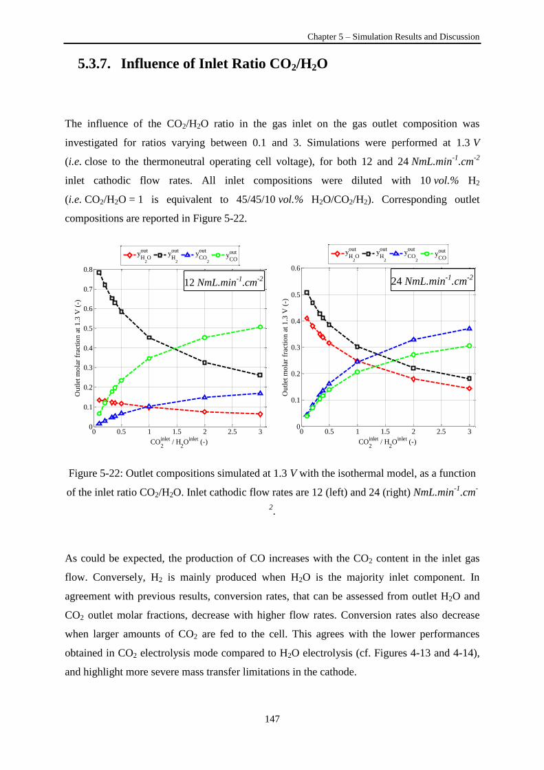
Chapter 5 – Simulation Results and Discussion
147
5.3.7. Influence of Inlet Ratio CO2/H2O
The influence of the CO2/H2O ratio in the gas inlet on the gas outlet composition was
investigated for ratios varying between 0.1 and 3. Simulations were performed at 1.3 V
(i.e. close to the thermoneutral operating cell voltage), for both 12 and 24 NmL.min-1
.cm-2
inlet cathodic flow rates. All inlet compositions were diluted with 10 vol.% H2
(i.e. CO2/H2O = 1 is equivalent to 45/45/10 vol.% H2O/CO2/H2). Corresponding outlet
compositions are reported in Figure 5-22.
Figure 5-22: Outlet compositions simulated at 1.3 V with the isothermal model, as a function
of the inlet ratio CO2/H2O. Inlet cathodic flow rates are 12 (left) and 24 (right) NmL.min-1
.cm-
2.
As could be expected, the production of CO increases with the CO2 content in the inlet gas
flow. Conversely, H2 is mainly produced when H2O is the majority inlet component. In
agreement with previous results, conversion rates, that can be assessed from outlet H2O and
CO2 outlet molar fractions, decrease with higher flow rates. Conversion rates also decrease
when larger amounts of CO2 are fed to the cell. This agrees with the lower performances
obtained in CO2 electrolysis mode compared to H2O electrolysis (cf. Figures 4-13 and 4-14),
and highlight more severe mass transfer limitations in the cathode.
0 0.5 1 1.5 2 2.5 30
0.1
0.2
0.3
0.4
0.5
0.6
0.7
0.8
CO2
inlet / H
2O
inlet (-)
Ou
tlet
mo
lar
frac
tio
n a
t 1
.3 V
(-)
yH
2O
outy
H2
outy
CO2
outy
CO
out
0 0.5 1 1.5 2 2.5 30
0.1
0.2
0.3
0.4
0.5
0.6
CO2
inlet / H
2O
inlet (-)
Ou
tlet
mo
lar
frac
tio
n a
t 1
.3 V
(-)
yH
2O
outy
H2
outy
CO2
outy
CO
out
12 NmL.min-1
.cm-2
24 NmL.min-1
.cm-2
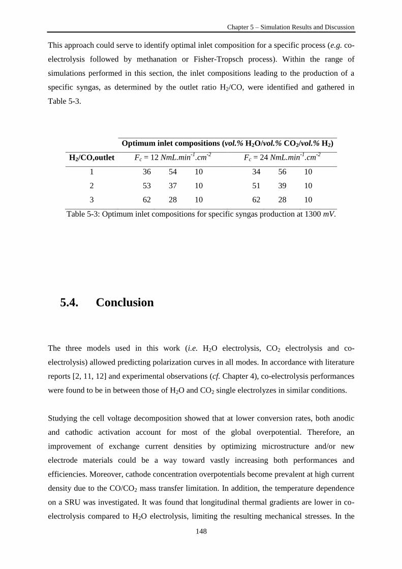
Chapter 5 – Simulation Results and Discussion
148
This approach could serve to identify optimal inlet composition for a specific process (e.g. co-
electrolysis followed by methanation or Fisher-Tropsch process). Within the range of
simulations performed in this section, the inlet compositions leading to the production of a
specific syngas, as determined by the outlet ratio H2/CO, were identified and gathered in
Table 5-3.
Optimum inlet compositions (vol.% H2O/vol.% CO2/vol.% H2)
H2/CO,outlet Fc = 12 NmL.min-1
.cm-2
Fc = 24 NmL.min-1
.cm-2
1 36 54 10 34 56 10
2 53 37 10 51 39 10
3 62 28 10 62 28 10
Table 5-3: Optimum inlet compositions for specific syngas production at 1300 mV.
5.4. Conclusion
The three models used in this work (i.e. H2O electrolysis, CO2 electrolysis and co-
electrolysis) allowed predicting polarization curves in all modes. In accordance with literature
reports [2, 11, 12] and experimental observations (cf. Chapter 4), co-electrolysis performances
were found to be in between those of H2O and CO2 single electrolyzes in similar conditions.
Studying the cell voltage decomposition showed that at lower conversion rates, both anodic
and cathodic activation account for most of the global overpotential. Therefore, an
improvement of exchange current densities by optimizing microstructure and/or new
electrode materials could be a way toward vastly increasing both performances and
efficiencies. Moreover, cathode concentration overpotentials become prevalent at high current
density due to the CO/CO2 mass transfer limitation. In addition, the temperature dependence
on a SRU was investigated. It was found that longitudinal thermal gradients are lower in co-
electrolysis compared to H2O electrolysis, limiting the resulting mechanical stresses. In the
Chapter 5 – Simulation Results and Discussion
149
exothermic part of the computed co-electrolysis polarization curves, the benefits from higher
temperature, which could have yielded higher current densities, are hindered by higher mass
transfer limitations than in H2O electrolysis. Indeed, a maximum current density was
simulated (i.e. about -2.2 A.cm-2
), resulting in large drops of conversion rates when the
cathodic flow rate was increased. Therefore, studies devoted to microstructure optimization of
the cell support to enhance CO/CO2 gas transport should constitute a promising way to
improve cell efficiency in co-electrolysis operation.
Results showed that CO2 can be electrochemically reduced in presence of H2O, in agreement
with experimental evidence of CO2 electrolysis feasibility (cf. Chapter 3). In the chosen, the
influence of the WGS reaction in CO production was elucidated. It is found that the chemical
reaction does not prevail over electrochemistry in conditions compatible with a Power-to-Gas
process at about 800°C. Even if inlets were chosen to favor the WGS reaction, it still did not
account for the majority of the global syngas production.
Co-electrolysis operating maps were computed for inlet composition 65/25/10 vol.%
H2O/CO2/H2. These highlight that optimal operating conditions could be mainly determined
by the conversion rate. In addition, the outlet ratio H2/CO depends on current density, inlet
cathodic flow rate and temperature. These parameters, to which one could add the cermet
thickness and general cell dimensions, could all be adjustable variables to obtain a specific
outlet gas composition, for a coupling with a specific process (e.g. Methanation reaction).
Finally, the co-electrolysis model proved to be an excellent tool to investigate the complex
and entangled phenomena occurring in an operating SOC.
Chapter 5 – Simulation Results and Discussion
150
5.5. References
1. X. Sun, M. Chen, S. H. Jensen, S. D. Ebbesen, C. Graves, and M. Mogensen, Thermodynamic
analysis of synthetic hydrocarbon fuel production in pressurized solid oxide electrolysis cells, Int.
J. Hydrog. Energy 37, 17101 (2012).
2. P. Kim-Lohsoontorn, N. Laosiripojana, and J. Bae, Performance of solid oxide electrolysis cell
having bi-layered electrolyte during steam electrolysis and carbon dioxide electrolysis, Curr.
Appl. Phys. 11, S223 (2011).
3. P. Kim-Lohsoontorn and J. Bae, Electrochemical performance of solid oxide electrolysis cell
electrodes under high-temperature coelectrolysis of steam and carbon dioxide, J. Power Sources
196, 7161 (2011).
4. S. H. Jensen, P. H. Larsen, and M. Mogensen, Hydrogen and synthetic fuel production from
renewable energy sources, Int. J. Hydrog. Energy 32, 3253 (2007).
5. P. Kazempoor and R. J. Braun, Model validation and performance analysis of regenerative solid
oxide cells: Electrolytic operation, Int. J. Hydrog. Energy 39, 2669 (2014).
6. J. Laurencin, D. Kane, G. Delette, J. Deseure, and F. Lefebvre-Joud, Modelling of solid oxide
steam electrolyser: Impact of the operating conditions on hydrogen production, J. Power Sources
196, 2080 (2011).
7. J. Laurencin, F. Lefebvre-Joud, and G. Delette, Impact of cell design and operating conditions on
the performances of SOFC fuelled with methane, J. Power Sources 177, 355 (2008).
8. F. Usseglio-Viretta, J. Laurencin, G. Delette, J. Villanova, P. Cloetens, and D. Leguillon,
Quantitative microstructure characterization of a Ni–YSZ bi-layer coupled with simulated
electrode polarisation, J. Power Sources 256, 394 (2014).
9. R. Suwanwarangkul, E. Croiset, E. Entchev, S. Charojrochkul, M. D. Pritzker, M. W. Fowler, P.
L. Douglas, S. Chewathanakup, and H. Mahaudom, Experimental and modeling study of solid
oxide fuel cell operating with syngas fuel, J. Power Sources 161, 308 (2006).
10. F. Usseglio-Viretta, Optimisation des performances et de la robustesse d’un électrolyseur à
hautes températures, (2014).
11. J. E. O’Brien, M. G. McKellar, C. M. Stoots, J. S. Herring, and G. L. Hawkes, Parametric study of
large-scale production of syngas via high-temperature co-electrolysis, Int. J. Hydrog. Energy 34,
4216 (2009).
12. C. Graves, S. D. Ebbesen, and M. Mogensen, Co-electrolysis of CO2 and H2O in solid oxide
cells: Performance and durability, Solid State Ion. 192, 398 (2011).

Chapter 5 – Simulation Results and Discussion
151

Chapter 6 – Conclusion
152
Chapter 6
Conclusion

Chapter 6 – Conclusion
153
Chapter 6 – Conclusion
154
Chapter 6
Conclusion
This work investigated the high temperature co-electrolysis of steam and carbon dioxide in
SOCs, and the relevance of this operating mode to produce storage units for carbon-free
electricity overproduction as well as CO2 valorization devices. Indeed, co-electrolysis should
enable the conversion of H2O and CO2 emitted by industries (such as nuclear power plants
and cement, energy, chemical, steel industries respectively) into syngas (H2+CO) and oxygen.
The syngas can, in turn, be converted into high added value storable products, such as
methane or synthetic liquid fuels (methanol or DME), while oxygen can be valorized and
used in industrial sites. To better understand the entangled phenomena occurring in a SOC
operated in co-electrolysis mode, the chemical and electrochemical response of typical
commercial cells was investigated using a coupled experimental and modeling approach.
An in-house co-electrolysis model was adapted from a previous one developed in steam
electrolysis. The model takes into account mass transfer, chemical, electrochemical and
thermal phenomena occurring inside the operating SOC. Furthermore, it was duplicated to
consider both radial and planar cell geometries, needed to be respectively representative of
experimental data acquired on a single cells as well as stack environments. Additionally, a
macroscopic representation of the electrochemical mechanism was proposed through the
introduction of a surface ratio parameter β. This parameter, which was expressed as a function
of local steam and carbon dioxide partial pressures, encompasses the coupled mechanisms
related to the simultaneous CO2 and H2O electro-reductions within the same cathodic active
layer.
In parallel to the numerical approach, numerous experimental tools were set up in this
investigation. A test bench dedicated to co-electrolysis measurements was designed based on
the laboratory feedbacks. After putting the test rig into service, its reliability was optimized.
Finally, a micro gas chromatograph was coupled to the test bench to analyze cell outlet
compositions.
Chapter 6 – Conclusion
155
Experimental polarization curves obtained in all electrolysis modes displayed typical
behaviors consistent with literature reports. Co-electrolysis performances were shown to lie
between those of H2O and CO2 single electrolyzes. Additionally, current densities as high as
-1.5 A.cm-2
were achieved in CO2 electrolysis on optimized cells. This result confirms the
possibility to electrochemically reduce CO2 in standard SOCs.
Single electrolysis and co-electrolysis models were experimentally validated on two types of
commercial Cathode Supported Cells (CSC), one of which had a well-known microstructure.
Experimental protocols were developed to highlight variations in cathodic overpotentials
through feeding composition and flow changes. Complete polarization curves were
investigated and compared to the simulation over a large range of cell voltages (from open
circuit voltages to steep limiting currents). A special attention was paid to avoid any
significant degradation during the protocols.
The good agreement between simulations and experiments in all electrolysis modes has
allowed confirming the models ability to predict polarization curves. In addition, gas analyses
were performed at OCV and in operation in order to respectively validate both the Water Gas
Shift (WGS) reaction kinetics and the expression of the surface ratio as a combination of local
H2O and CO2 partial pressures.
A good consistency between simulated and experimental cell outlet compositions was
highlighted over the complete range of current densities. Furthermore, a sensitivity analysis
was performed by changing the expression of β. It has been found that any modifications in
the definition of this parameter lead to a large disagreement between model predictions and
experimental gas composition analysis. In such conditions, the co-electrolysis model loses its
relevance. In other words, only one expression of the surface ratio is liable to accurately
model and predict the co-electrolysis experiments. This result tends to prove the underlying
physical meanings of β and shows that the model can be used over a large range of gas
composition with a high level of confidence.
Detailed analyses of numerous simulations led to assess the relative influence of the WGS
reaction over CO production in co-electrolysis operations. It was demonstrated that, within
the range of this study, the chemical reaction does not prevail over CO2 electrolysis, as long
as the cell current density is sufficiently high. Since such currents were obtained for cell
voltages as low as 1.1 V, this statement would apply to realistic co-electrolysis operation.
Such conclusion was also shown to stand with inlet compositions favoring the WGS reaction.
It should be emphasized here that a limited influence of the WGS reaction contradicts some
Chapter 6 – Conclusion
156
literature reports. Indeed, most of these studies have concluded that CO2 electrolysis is
negligible since they have focused their investigation on low current densities. According to
the simulation analysis, the limited influence of the WGS reaction is believed to arise from
the reaction changing direction within the cathode 2D geometry so that its production is
globally balanced
Further analysis of the simulations highlighted that, due to the presence of CO/CO2 in CO2
and co-electrolysis modes, mass transfer through the porous cathode is a limiting process that
induces large concentration overpotentials. This was confirmed by the decreased in cell
performances experimentally evidenced in these modes of operation compared to single H2O
electrolysis. Therefore, a cathode microstructure specifically optimized for co-electrolysis
operation seems to be a major way toward improved performances. Additionally, it was
shown that over the range of realistic co-electrolysis operation, activation overpotentials
account for the majority of the cell voltage increase. Such issue could be mitigated through
triple phase boundary lengths density increase and/or more electroactive electrode materials.
Once validated, the co-electrolysis model was used to determine operating maps for a
technologically relevant inlet composition (i.e. 65/25/10 vol.% H2O/CO2/H2). The simulations
were carried out over a wide range of inlet flows and cell polarizations. This investigation
evidenced that inlet composition, flow rate, temperature and current density are the most
contributing factors that governs the outlet gas composition. Consequently, by taking
advantages of the simulated cartographies, optimal operating conditions were identified.
Additionally, global temperature variations and longitudinal thermal gradients were found to
be limited in co-electrolysis operation, compared to H2O electrolysis. From this statement, it
has been claimed that the range of acceptable operating conditions in co-electrolysis mode
could be wider than the one previously identified in steam electrolysis, and might simplify the
thermal management of the co-electrolyzer.
Many different research paths could complete this work. First, several additional series of
studies could be performed to improve the model range of applicability. For instance, the
thermal dependence of key parameters such as the surface ratio β could be investigated.
Moreover, thanks to the micro modeling approach depicted in [1], the dependence of the
“apparent” current densities with electrode microstructure, atmosphere or even polarization
could be estimated.
Besides, the underlying mechanisms of co-electrolysis process included in the macroscopic
parameter β needs to be clarified. For this purpose, the elementary reactions pathway and the

Chapter 6 – Conclusion
157
associated rate-determining steps for co-electrolysis should be established. It could be propose
to identify the most plausible mechanisms by coupling the microscopic modeling approach
with electrochemical measurements performed on symmetrical cells in a 3 electrodes
configuration (polarization curves and impedance diagrams investigations in co-electrolysis
and single electrolysis modes).
Also, the WGS kinetics constants (pre-exponential and activation energy) implemented the
model, could be further validated through accurate chemical rates measurements, based on
non-equilibrium outlet compositions. These could not be done in this work due to test bench
limitations.
Furthermore, the gaps obtained in H2O electrolysis at high current densities could probably be
improved through H2 diffusion coefficients optimization and/or by taking into account some
of the potential dependences already evoked. In addition, the evolution in time of co-
electrolysis performances must be investigated. Indeed, this technology cannot become viable
if degradation rates are too high. Such optimization requires a better comprehension of the
microscopic co-electrolysis electrochemical mechanism.
Finally, a deep investigation on the influence of pressurized co-electrolysis must be
conducted. Indeed, it has been proposed in an industrial flow-chart to associate a co-
electrolyzer with a methanation reactor, which operates at high pressure. Technical
assessments of this industrial process have suggested that large gains in efficiency and cost
could be achieved when both devices have similar operating conditions. Nonetheless, the
beneficial or detrimental effect of pressure on the co-electrolysis process has to be carefully
estimated. For this purpose, the effect of pressure should be taken into account in the co-
electrolysis model. It is expected that pressure could impact the electrochemistry as well as
the gas mass transfer. Moreover, the catalytic reaction of methane formation in the cathode
should be implemented in the model. Also, the risk of carbon should constitute an important
issue that should be studied.
1. E. Lay-Grindler, J. Laurencin, G. Delette, J. Aicart, M. Petitjean, and L. Dessemond, Micro
modelling of solid oxide electrolysis cell: From performance to durability, Int. J. Hydrog. Energy
38, 6917 (2013).

Chapter 7 – Appendix
158
Chapter 7
Appendix

Chapter 7 – Appendix
159
Chapter 7 – Appendix
160
Chapter 7
Appendix
7.1. Hysteresis on Optimized Cell ........................................................................................... 161
7.1.1. Influence of Composition and Time ......................................................................... 161
7.1.2. Influence of Limiting Current .................................................................................. 163
7.1.3. Conclusion .................................................................................................................. 164
7.2. Cell Degradation in Co-Electrolysis................................................................................. 165
7.2.1. Durability Experiment : 900 h at -1 A.cm-2
............................................................. 165
7.2.2. MEB Analysis ............................................................................................................ 167
7.3. Steam Electrolysis Operating Maps ................................................................................. 171
7.4. References .......................................................................................................................... 174
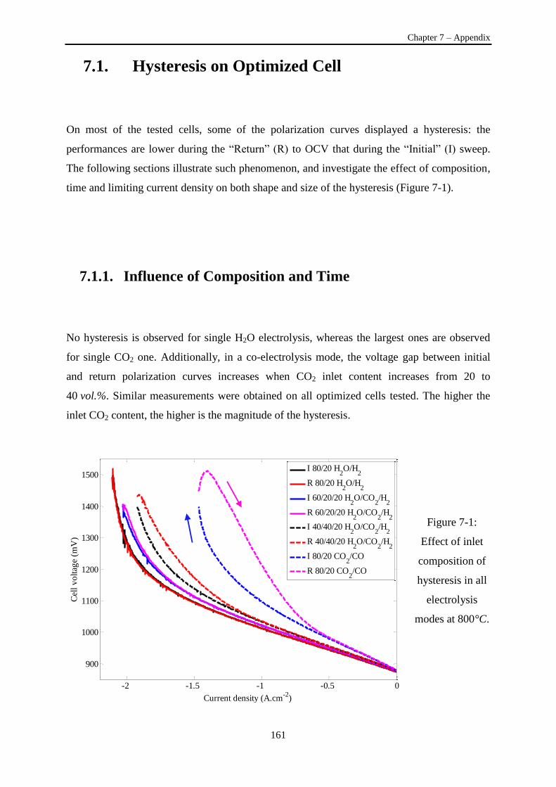
Chapter 7 – Appendix
161
7.1. Hysteresis on Optimized Cell
On most of the tested cells, some of the polarization curves displayed a hysteresis: the
performances are lower during the “Return” (R) to OCV that during the “Initial” (I) sweep.
The following sections illustrate such phenomenon, and investigate the effect of composition,
time and limiting current density on both shape and size of the hysteresis (Figure 7-1).
7.1.1. Influence of Composition and Time
No hysteresis is observed for single H2O electrolysis, whereas the largest ones are observed
for single CO2 one. Additionally, in a co-electrolysis mode, the voltage gap between initial
and return polarization curves increases when CO2 inlet content increases from 20 to
40 vol.%. Similar measurements were obtained on all optimized cells tested. The higher the
inlet CO2 content, the higher is the magnitude of the hysteresis.
Figure 7-1:
Effect of inlet
composition of
hysteresis in all
electrolysis
modes at 800°C.
-2 -1.5 -1 -0.5 0
900
1000
1100
1200
1300
1400
1500
Current density (A.cm-2
)
Cel
l v
olt
age
(mV
)
I 80/20 H2O/H
2
R 80/20 H2O/H
2
I 60/20/20 H2O/CO
2/H
2
R 60/20/20 H2O/CO
2/H
2
I 40/40/20 H2O/CO
2/H
2
R 40/40/20 H2O/CO
2/H
2
I 80/20 CO2/CO
R 80/20 CO2/CO
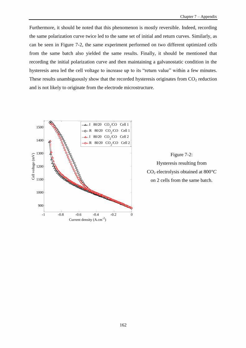
Chapter 7 – Appendix
162
Furthermore, it should be noted that this phenomenon is mostly reversible. Indeed, recording
the same polarization curve twice led to the same set of initial and return curves. Similarly, as
can be seen in Figure 7-2, the same experiment performed on two different optimized cells
from the same batch also yielded the same results. Finally, it should be mentioned that
recording the initial polarization curve and then maintaining a galvanostatic condition in the
hysteresis area led the cell voltage to increase up to its “return value” within a few minutes.
These results unambiguously show that the recorded hysteresis originates from CO2 reduction
and is not likely to originate from the electrode microstructure.
Figure 7-2:
Hysteresis resulting from
CO2 electrolysis obtained at 800°C
on 2 cells from the same batch.
-1 -0.8 -0.6 -0.4 -0.2 0
900
1000
1100
1200
1300
1400
1500
Current density (A.cm-2
)
Cel
l v
olt
age
(mV
)
I 80/20 CO2/CO Cell 1
R 80/20 CO2/CO Cell 1
I 80/20 CO2/CO Cell 2
R 80/20 CO2/CO Cell 2
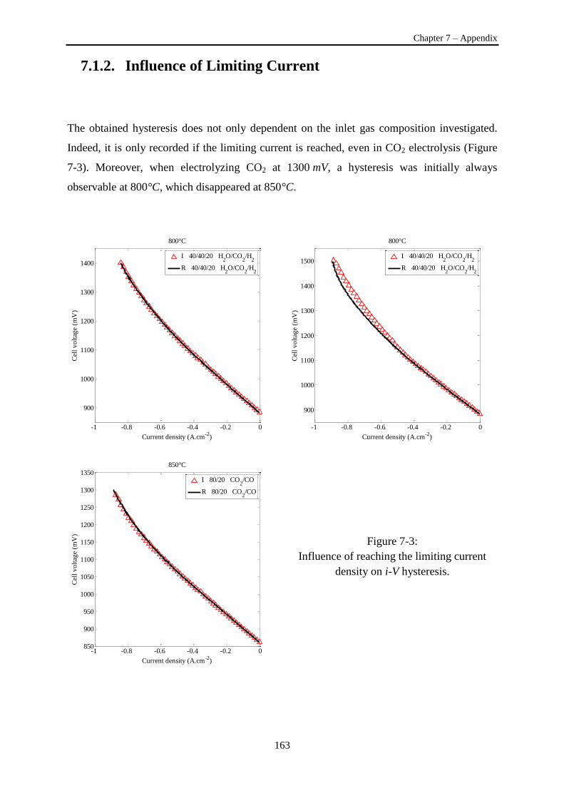
Chapter 7 – Appendix
163
7.1.2. Influence of Limiting Current
The obtained hysteresis does not only dependent on the inlet gas composition investigated.
Indeed, it is only recorded if the limiting current is reached, even in CO2 electrolysis (Figure
7-3). Moreover, when electrolyzing CO2 at 1300 mV, a hysteresis was initially always
observable at 800°C, which disappeared at 850°C.
Figure 7-3:
Influence of reaching the limiting current
density on i-V hysteresis.
-1 -0.8 -0.6 -0.4 -0.2 0
900
1000
1100
1200
1300
1400
Current density (A.cm-2
)
Cel
l v
olt
age
(mV
)
800°C
I 40/40/20 H2O/CO
2/H
2
R 40/40/20 H2O/CO
2/H
2
-1 -0.8 -0.6 -0.4 -0.2 0
900
1000
1100
1200
1300
1400
1500
Current density (A.cm-2
)
Cel
l v
olt
age
(mV
)
800°C
I 40/40/20 H2O/CO
2/H
2
R 40/40/20 H2O/CO
2/H
2
-1 -0.8 -0.6 -0.4 -0.2 0850
900
950
1000
1050
1100
1150
1200
1250
1300
1350
Current density (A.cm-2
)
Cel
l v
olt
age
(mV
)
850°C
I 80/20 CO2/CO
R 80/20 CO2/CO
Chapter 7 – Appendix
164
7.1.3. Conclusion
Since the hysteresis is observed once the limiting current is be reached, this CO2 related
phenomenon is likely to be independent of diffusion processes through the porous electrode.
Indeed, the temperature variation investigaetd has a limited impact on gaseous diffusion,
whereas this phenomenon vanished by increasing the temperature by 50°C.
To the best of my current knowledge, there are limited experimental reports concerning CO2
electrolysis, none of which display return curves. However, the literature is much more
extensive about CO oxidation. Indeed, Holtappels et al. [1] have reported a highly dynamical
CO oxidation, with multiple and periodically changing reaction rates, believed to be related to
passivation and reactivation of active sites. These observations could be coherent with reports
of changes in number of relaxation times [2] and mechanism [3] depending on 2
/CO COP P
ratios. Accordingly, a change CO2 adsorption and/or CO desorption processes at high CO
contents (i.e. limiting current density) could explain the observed hysteresis. Such slower
mechanism, becoming limiting as COP increases, could also explain the time dependence
observed.
Additional experiments in the hysteresis section of polarization curves are required to further
understand this dynamic phenomenon. For example, EIS measurements under polarization
could give insights on a variation of elementary steps in electrolysis mode. However, it should
be emphasized that this phenomenon does not affect the predictive ability of the co-
electrolysis model developed in this work (cf. Chapter 3). Indeed, from a technological point
of view (cf. Chapter 5), imposing a limiting current is not optimal since degradation rates
should be increased, and performances should suffer from higher cathodic concentration
overpotential. In addition, special interest is currently given to inlet composition
65/25/10 vol.% H2O/CO2/H2, as it can lead to methane production. As previously showed
(Figure 7-1), only a very limited hysteresis could sometimes be observed in these conditions.
Chapter 7 – Appendix
165
7.2. Cell Degradation in Co-Electrolysis
7.2.1. Durability Experiment : 900 h at -1 A.cm-2
One of the optimized cells (cf. Chapter 4) operated in H2O electrolysis and H2O+CO2 co-
electrolysis modes to assess the corresponding degradation rates. After initial start-up
procedures (cf. Chapter 3), polarization curves were recorded. Subsequently, the cell was
operated in a galvanostatic mode at -1 A.cm-2
and 24 NmL.min-1
.cm-2
cathodic flow, first
during 259 h with 90/10 vol.% H2O/H2 (+20% N2), then 643 h with 65/25/10 vol.%
H2O/CO2/H2. Additional evaluations of performances were performed between both modes
and at the end of the experiment. The voltage increase was deduced from the time evolution
of the cell voltage, and the extrapolation of these results led to assess degradation rates per kh
(Figure 7-4).
Excluding the initial voltage jump, operating the cell in H2O electrolysis mode lead to a quasi
linear degradation rate of +8.8 %.kh-1
. Conversely, the slope of the cell voltage evolution
changes abruptly in co-electrolysis mode, leading to 2 very different degradation rates: +19.3
and 8.4 %.kh-1
respectively. Many additional experiments are required to further investigate
degradation rates in co-electrolysis mode, and to draw any meaningful conclusions. In
addition, there are very few related literature reports, and none at such a high current density.
However, the as-recorded results suggest that co-electrolysis could result in higher but
comparable degradation rates compared to H2O electrolysis.
During the 643 h of co-electrolysis operation, steam outlet mass balance was performed (see
4.2.7 for additional details), as well as µGC measurements. Results shown in Table 7-1
highlight yet again the agreement between simulated and experimental data, and therefore the
model ability to predict outlet composition in operating conditions. It is worth noting here that
in the specific case of this experiment, computing the H2O and CO2 conversions from
Faraday’s law and the model gives the same result. Such observation arises from the specific
set of operating conditions investigated here, and has not been observed anywhere else is this
work.
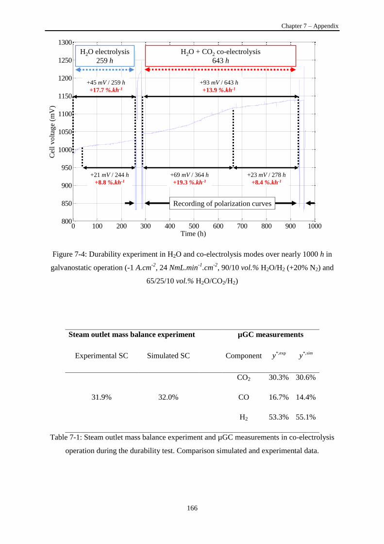
Chapter 7 – Appendix
166
Figure 7-4: Durability experiment in H2O and co-electrolysis modes over nearly 1000 h in
galvanostatic operation (-1 A.cm-2
, 24 NmL.min-1
.cm-2
, 90/10 vol.% H2O/H2 (+20% N2) and
65/25/10 vol.% H2O/CO2/H2)
Steam outlet mass balance experiment µGC measurements
Experimental SC Simulated SC Component *,expy *,simy
31.9% 32.0%
CO2 30.3% 30.6%
CO 16.7% 14.4%
H2 53.3% 55.1%
Table 7-1: Steam outlet mass balance experiment and µGC measurements in co-electrolysis
operation during the durability test. Comparison simulated and experimental data.
0 100 200 300 400 500 600 700 800 900 1000800
850
900
950
1000
1050
1100
1150
1200
1250
1300
Time (h)
Cel
l v
olt
age
(mV
)
Recording of polarization curves
H2O electrolysis
259 h
H2O + CO2 co-electrolysis
643 h
+45 mV / 259 h
+17.7 %.kh-1
+93 mV / 643 h
+13.9 %.kh-1
+21 mV / 244 h
+8.8 %.kh-1
+69 mV / 364 h
+19.3 %.kh-1
+23 mV / 278 h
+8.4 %.kh-1
Chapter 7 – Appendix
167
7.2.2. MEB Analysis
Scanning Electrons Microscope (SEM) and Energy Dispersive Spectrometry (EDS)
cartographies were performed on three optimized cell: a reference cell with a fully reduced
cermet (referred to as cell 1 here), the cell used in section 4.3 (cell 2), and the cell presented in
the previous paragraph that was operated during 9000 h (cell 3). Contrary to both latter cells,
the reference cell was not operated before examinations. The vicinity of the
cathode/electrolyte interface was observed in order to investigate carbon deposition.
Fractographies of the cells were examined using a SEM FEG (LEO 1530) equipped with a
high resolution INLENS detector. Results obtained on cell 1, 2 and 3 are displayed on Figures
7-5, 7-6 and 7-7, respectively.
First, no explicit carbon deposition could be detected through the MEB examinations and
chemical analyses. However, this does not necessarily means that such phenomenon did not
occur. Indeed, late polarization curves in H2O electrolysis performed on cell 2 and 3 could
have oxidized any potential solid carbon.
Furthermore, although they were operated during ≈ 400 h and ≈ 900 h respectively, cell 2 and
3 seem to display similar microstructures, significantly different from the reference
observations. Indeed, Nickel particles seem bigger and their distribution less homogeneous in
operated cell compared to initial examinations. This could be sign of Ni aggregation, an
identified degradation phenomenon [4]. In addition, these modified microstructures also
appear to change from the center of the cell (i.e. inlet) to the active area outlet.
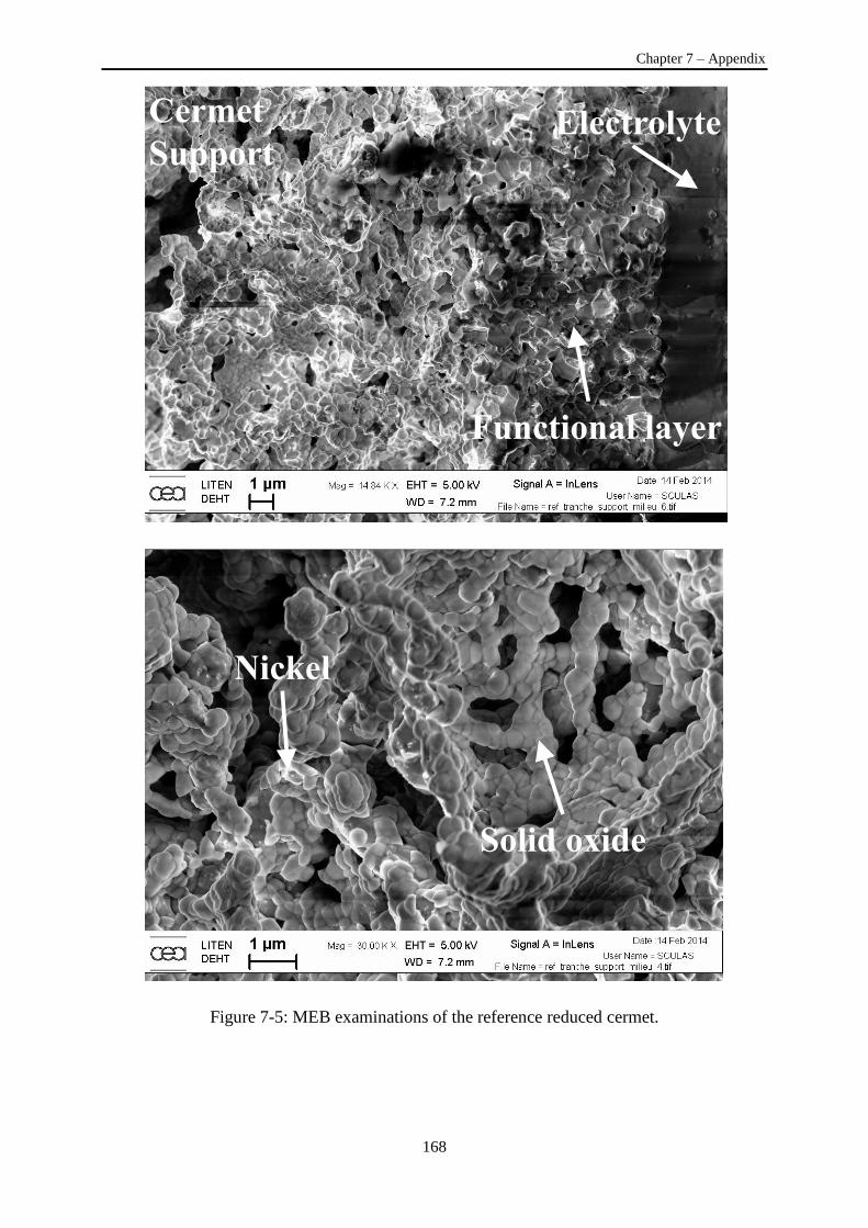
Chapter 7 – Appendix
168
Figure 7-5: MEB examinations of the reference reduced cermet.
Electrolyte
Functional layer
Cermet
Support
Solid oxide
Nickel
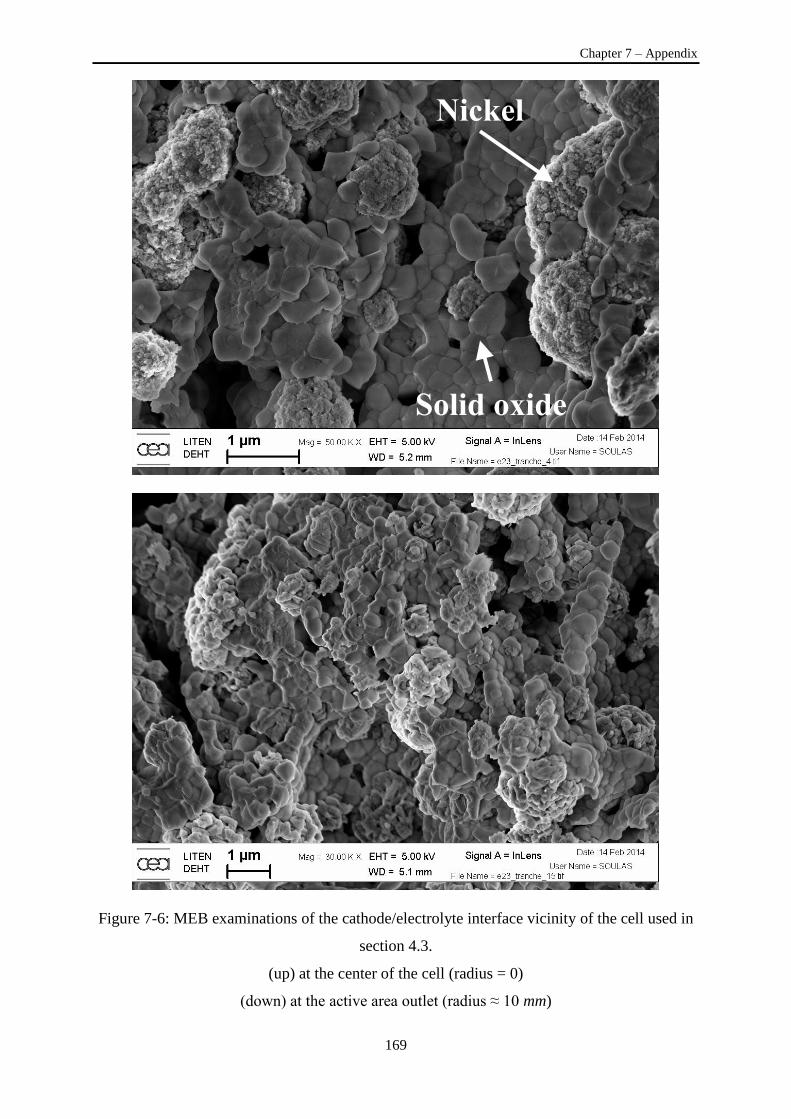
Chapter 7 – Appendix
169
Figure 7-6: MEB examinations of the cathode/electrolyte interface vicinity of the cell used in
section 4.3.
(up) at the center of the cell (radius = 0)
(down) at the active area outlet (radius ≈ 10 mm)
Solid oxide
Nickel
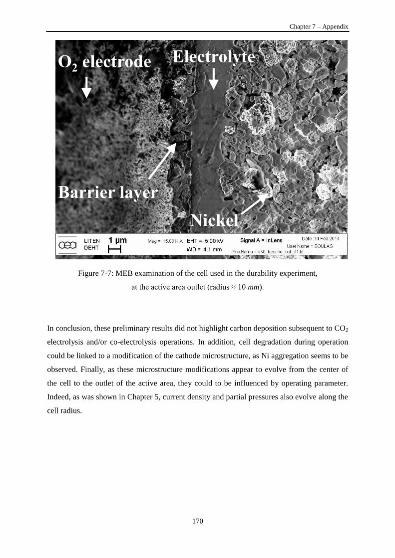
Chapter 7 – Appendix
170
Figure 7-7: MEB examination of the cell used in the durability experiment,
at the active area outlet (radius ≈ 10 mm).
In conclusion, these preliminary results did not highlight carbon deposition subsequent to CO2
electrolysis and/or co-electrolysis operations. In addition, cell degradation during operation
could be linked to a modification of the cathode microstructure, as Ni aggregation seems to be
observed. Finally, as these microstructure modifications appear to evolve from the center of
the cell to the outlet of the active area, they could to be influenced by operating parameter.
Indeed, as was shown in Chapter 5, current density and partial pressures also evolve along the
cell radius.
Nickel
ElectrolyteO2 electrode
Barrier layer
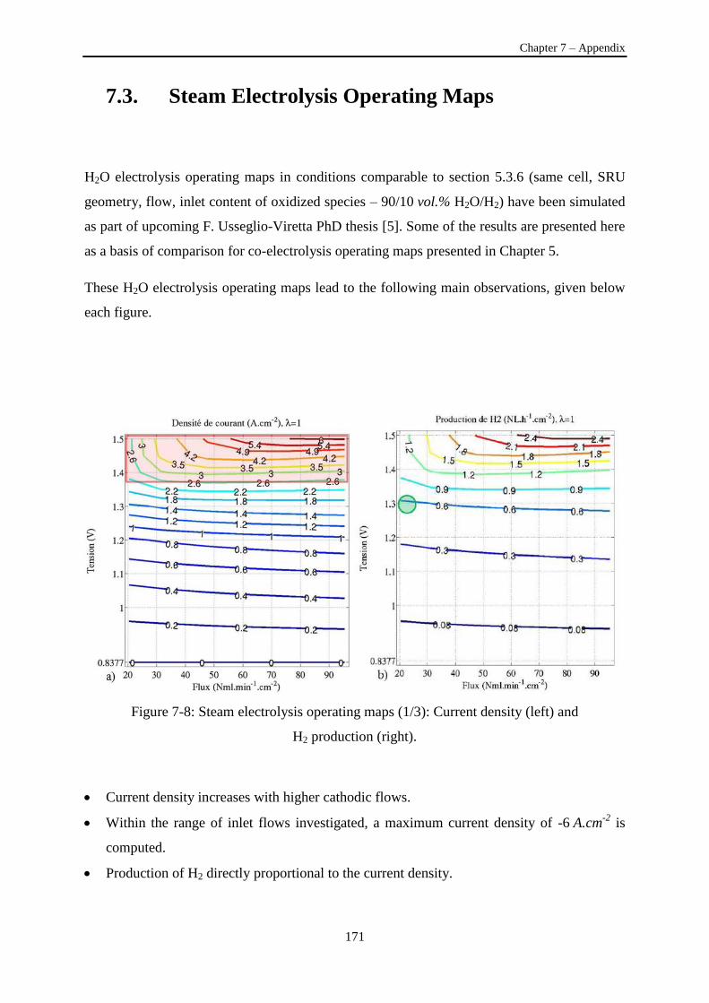
Chapter 7 – Appendix
171
7.3. Steam Electrolysis Operating Maps
H2O electrolysis operating maps in conditions comparable to section 5.3.6 (same cell, SRU
geometry, flow, inlet content of oxidized species – 90/10 vol.% H2O/H2) have been simulated
as part of upcoming F. Usseglio-Viretta PhD thesis [5]. Some of the results are presented here
as a basis of comparison for co-electrolysis operating maps presented in Chapter 5.
These H2O electrolysis operating maps lead to the following main observations, given below
each figure.
Figure 7-8: Steam electrolysis operating maps (1/3): Current density (left) and
H2 production (right).
Current density increases with higher cathodic flows.
Within the range of inlet flows investigated, a maximum current density of -6 A.cm-2
is
computed.
Production of H2 directly proportional to the current density.
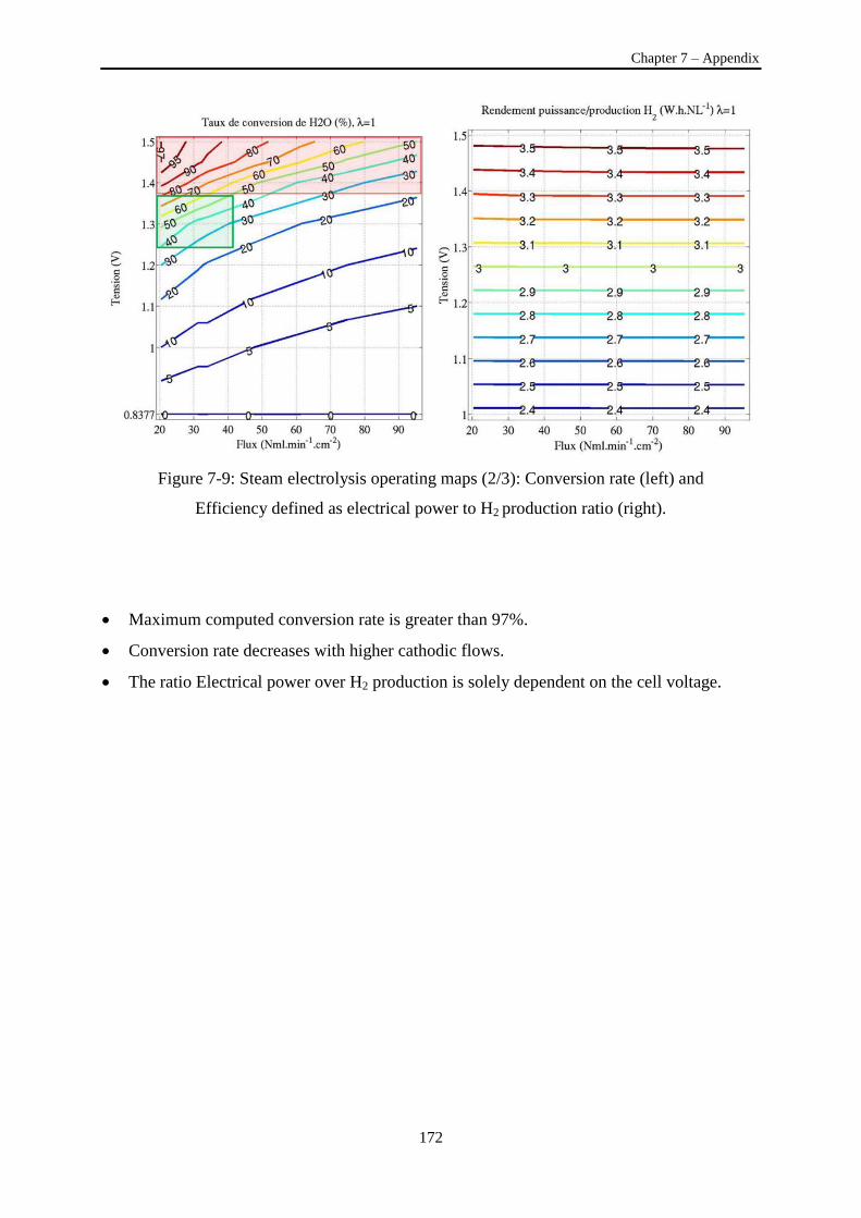
Chapter 7 – Appendix
172
Figure 7-9: Steam electrolysis operating maps (2/3): Conversion rate (left) and
Efficiency defined as electrical power to H2 production ratio (right).
Maximum computed conversion rate is greater than 97%.
Conversion rate decreases with higher cathodic flows.
The ratio Electrical power over H2 production is solely dependent on the cell voltage.
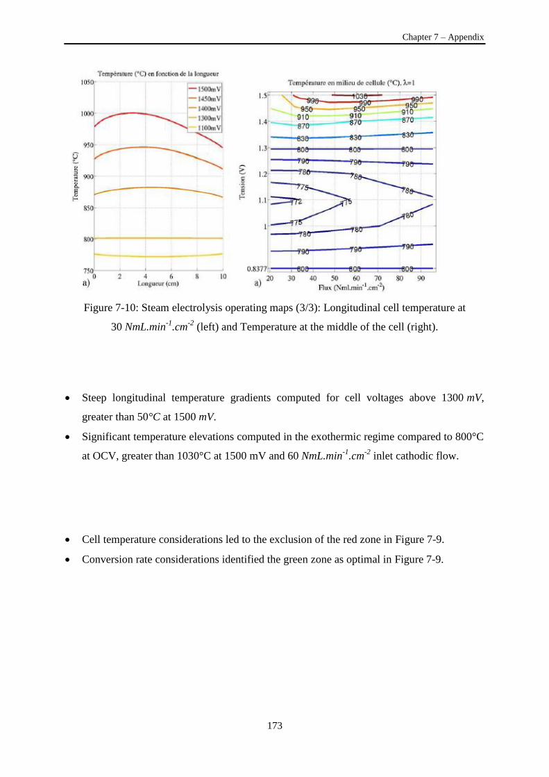
Chapter 7 – Appendix
173
Figure 7-10: Steam electrolysis operating maps (3/3): Longitudinal cell temperature at
30 NmL.min-1
.cm-2
(left) and Temperature at the middle of the cell (right).
Steep longitudinal temperature gradients computed for cell voltages above 1300 mV,
greater than 50°C at 1500 mV.
Significant temperature elevations computed in the exothermic regime compared to 800°C
at OCV, greater than 1030°C at 1500 mV and 60 NmL.min-1
.cm-2
inlet cathodic flow.
Cell temperature considerations led to the exclusion of the red zone in Figure 7-9.
Conversion rate considerations identified the green zone as optimal in Figure 7-9.
Chapter 7 – Appendix
174
7.4. References
1. P. Holtappels, L. G. J. De Haart, U. Stimming, I. C. Vinke, and M. Mogensen, Reaction of
CO/CO2 gas mixtures on Ni–YSZ cermet electrodes, J. Appl. Electrochem. 29, 561 (1999).
2. F. Boulenouar, K. Yashiro, M. Oishi, A. Kaimai, Y. Nigara, T. Kawada, and J. Mizusaki,
Electrochemical Oxidation of CO in a CO-CO2 System at the Interface of Ni Grid Electrode/YSZ
Electrolyte, Electrochem Soc Ser. 759 (2001).
3. V. Yurkiv, A. Utz, A. Weber, E. Ivers-Tiffée, H.-R. Volpp, and W. G. Bessler, Elementary kinetic
modeling and experimental validation of electrochemical CO oxidation on Ni/YSZ pattern anodes,
Electrochimica Acta 59, 573 (2012).
4. P. Moçoteguy and A. Brisse, A review and comprehensive analysis of degradation mechanisms of
solid oxide electrolysis cells, Int. J. Hydrog. Energy 38, 15887 (2013).
5. F. Usseglio-Viretta, Optimisation des performances et de la robustesse d’un électrolyseur à hautes
températures, (2014).

Chapter 7 – Appendix
175

Abstract
This work investigates the high temperature co-electrolysis of H2O and CO2 in Solid Oxide
Cells. A detailed model was developed, encompassing electrochemical, chemical, thermal and
mass transfer phenomena, and introducing a macroscopic representation of the co-electrolysis
mechanism. This model allows predicting the performances and outlet compositions in single
cell and stack environments. An experimental validation protocol was implemented on two
types of commercial Cathode Supported Cells, ranging from polarization curves, obtained in
single and co-electrolysis modes, to micro gas analyses. These tests aimed both at determining
the different exchange current densities, representative of the kinetics of electrochemical
reactions, and validating the simulated cell global behavior and mechanism proposed.
Comprehensive analysis of the simulations led to the identification of limiting processes and
paths for optimization, as well as to the establishment of co-electrolysis operating maps.
Résumé
Cette étude porte sur la co-électrolyse de H2O et CO2 à 800°C dans une cellule à oxydes
solides. Un modèle détaillé a été développé afin de rendre compte des phénomènes
électrochimiques, chimiques, thermiques et de transferts de matière, et introduisant une
représentation macroscopique du mécanisme de co-électrolyse. Il permet d’estimer les
performances et les compositions en sortie de cellule. Un protocole expérimental, visant à
valider les principales hypothèses de ce modèle, a été appliqué à deux types de cellule
commerciale à cathode support. À partir de courbes de polarisations, obtenues en électrolyse
et en co-électrolyse, ainsi que d’analyses gaz, les densités de courant d’échange, illustrant les
cinétiques électrochimiques, ont pu être estimées, et le mécanisme proposé a pu être validé.
L’analyse des simulations a permis l’identification des processus limitant la co-électrolyse, la
proposition de voies d’optimisation et l’établissement des cartographies de fonctionnement.