MOBILITY, URBAN SPRAWL AND ENVIRONMENTAL … · ENVIRONMENTAL RISKS IN BRAZILIAN URBAN AGGLOMERATIONS: CHALLENGES FOR URBAN ... tific and Technological ... transportation is also

MOBILITY, URBAN SPRAWL AND ENVIRONMENTAL RISKS IN BRAZILIAN

URBAN AGGLOMERATIONS: CHALLENGES FOR URBAN

SUSTAINABILITY1

Ricardo OJIMA

Post-doctoral Fellow, State of São Paulo Research Foundation (FAPESP); Collaborating Researcher, Population Studies Center, University of Campinas (Unicamp),

Researcher at the João Pinheiro Foundation, Brazil

Daniel Joseph HOGAN

Professor of Demography and Geography, University of Campinas (Unicamp), Brazil

Abstract Studies of uncontrolled expansion of urban land use mention innumerable social, economic and environmental impacts. Among the principal factors considered in terms of urban sprawl and the consumption of natural resources is the intensive use of individual automobile transportation. While this characteristic may be seen as both cause and conse-quence, the bottom line is that the greater the distances between different spheres of daily life, such as work, residence, study or shopping, the greater the demand for automobile transpor-tation. A sprawl index was created to identify this process in Brazilian urban agglomera-tions. The index is constructed with a set of sprawl factors identified in the international ―――― 1. This paper was part of the doctoral research of Ricardo Ojima under the su-pervision of Daniel J. Hogan, with financial support of National Council for Scien-tific and Technological Development (CNPq), and the post-doctoral research, with financial support of the State of São Paulo Research Foundation (FAPESP), Brazil.

This Chapter is from the volume: de Sherbiniin, A., A. Rahman, A. Barbieri, J.C. Fotso, and Y. Zhu (eds.). 2009. Urban Population-Environment Dynamics in the Developing World: Case Studies and Lessons Learned. Paris: Committee for International Cooperation in National Research in Demography (CICRED) (316 pages). Available at http://www.populationenvironmentresearch.org/workshops.jsp#W2007

282 RICARDO OJIMA AND DANIEL J. HOGAN

literature as important measures of sprawl-like situations. Geographic Information Systems (GIS) were also used to create spatial indices, such as urban density and a spatial dissimi-larity index. Today’s city has a more and more complex structure, above all considering the ramification of urban networks, the interaction of economic flows, the intensification of population mobility and changes in consumption patterns. An agglomeration may therefore take on different forms as it disperses in space and these different forms may have distinct social and environmental impacts. Key words: Urban sprawl; Environment; Sustainability. 1. Introduction According to United Nations projections, the world’s urban popu-lation will reach more than 50% in 2008, with the most important change occurring in developing countries. As a major component of modernization, urbanization has long occupied the attention of con-temporary social theorists, who have given much consideration to the radical changes at the foundations of modernity. Of central importance in the study of urbanization and environment is that globalization processes are seen both to destroy earlier structures and to offer solu-tions for certain perplexing paradoxes of contemporary life. The envi-ronmental dilemma, as a second major component of modernization is an unequivocal demonstration of this ambiguity in the 21st century be-cause it represents the conflicts of the production-consumption rela-tion. Thus, environmental debates stress the evidence of the ‘side-effects’ of urban-industrial processes and products. The concomitant occurrence of urbanization and environmental change endangers basic conditions of survival, changes ways of life and puts into question the belief of the superior rationality of experts. In this sense, global environmental risks express the challenges of such changes through global warming and its impacts on populations. This situation may be better observed in the complexity of urban con-texts around the world, including most of the urban agglomerations of developing countries. In Brazil, migration to urban areas occurred rap-idly in the nineteen seventies and by late 20th century had begun to pre-sent signs of an important transformation. Metropolitan areas that had grown in earlier decades are now losing centrality. New urban agglom-erations come to be the preferred destinations of urban-urban migra-

MOBILITY, URBAN SPRAWL AND ENVIRONMENTAL RISKS… 283

tion. In this second “urban transition”, urban sprawl is one of the signs of a new spatial relationship of production and consumption. Brazilian sprawl differs from that of the United States because there is an overlay of social processes that led to these urban forms. In the first urban transition, rural-urban migration was most important and the relationship between urbanization and production was mostly obvious. Today, urban-urban migration reveals new social forces which are leading to new urban forms: consumption of space follows the global urban tendency, in which regions and not cities are the most important scale of everyday life. The recent tendencies of the world urbanization process in a con-text of globalized markets point to a situation in which regions (as op-posed to specific localities) emerge as economic and political arenas with greater autonomy of action at national and global levels. City-regions constitute nodes which express a new social, economic and political order which, far from dissolution of regional importance re-sulting from the globalization process, become increasingly central to modern life. Urbanization, then, widens its scope beyond the image of the chaotic city which grows like an amoeba. The image is replaced by one of a polynucleated city, fragmented, with low densities, over wide-ranging territorial extensions, but at the same time more and more in-tegrated. Studies concerned with this uncontrolled expansion of urban land use mention innumerable social, economic and environmental impacts. Among the principal factors considered in terms of urban sprawl and the consumption of natural resources is the intensive use of individual automobile transportation. While this characteristic may be seen as both cause and consequence, the bottom line is that the greater the distances between different spheres of daily life, such as work, resi-dence, study or shopping, the greater the demand for automobile transportation. This is part of the growth in demand for fossil fuels as the princi-pal energy matrix of the modern world, a process with many different consequences. In the case of sprawl, the growing use of automobile transportation is also associated with an increase in air pollution. In this context, this paper discusses the recent changes that have occurred in Brazilian urban agglomerations, arguing that population mobility (migration and commuting) play an important role in determining demographic changes, in particular sprawl-like urbanization processes.


Most urban sprawl studies analyze the relationships between urbaniza-tion and environmental change in developed countries, but there is a need for efforts to treat these questions in developing countries. This paper will focus on the relations between population mobility and ur-ban form in Brazilian urban agglomerations using demographic data provided by the national Census Bureau (IBGE) to identify the most sprawling areas and the consequences for urban quality of life. Commuting data has not been commonly used in Brazilian urban studies, probably because it has not seemed to be a relevant phenome-non until recent years. These data began to be used intensively only in the last ten years as commuting increased throughout Brazil. This in-crease is associated with the expansion of urbanized areas in a new ur-ban morphology associated to the sprawl model. Despite the slowing of urban population growth in recent years, the physical size of urban areas is now increasing in many agglomerations of the country. A sprawl index was created to identify this process in each urban agglomeration. The index is constructed with a set of several sprawl factors identified in the international literature as important measures of sprawl-like situations, seeking to adapt it to the Brazilian context. Geographic Information Systems (GIS) were also used to create spatial indices, such as urban density and a spatial fragmentation index. To-day’s city has an increasingly complex structure, above all considering the ramification of urban networks, the interaction of economic flows, the intensification of population mobility and changes in consumption patterns. An agglomeration may therefore take on different forms as it disperses in space and these different forms may have distinct social and environmental impacts. 2. The Brazilian urban context: commuting and sprawl In a period of sixty years, Brazil’s urban population has increased from 30% to 80% of total population, the urban transition having been made in the mid-sixties. The urban transition, as in other countries of Latin America, occurred in a unique context: after developed coun-tries, but before most developing countries. Despite continuous urbanization, social and economic drivers of this process changed in the last years of the 20th century. During the first years of the urban transition, long-distance migration prevailed,


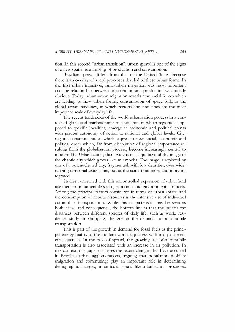
Figure 1 – Urban population (%), Brazil (1940-2000)

31,336,2

44,7

55,9

67,6

75,681,3

0

10

20

30

40

50

60

70

80

90

1940 1950 1960 1970 1980 1991 2000Year

% U

rban

Pop

ulat

ion

Source: IBGE, Demographic censuses 1940-2000. especially the Northeast-Southeast flow. Today, urban-urban migration has assumed the major role in spatial mobility. Commuting is increas-ing in metropolitan areas and has become part of individual strategies to reduce social, economic and environmental risk. Giddens (1991) argues that personal life and the social ties that it involves are deeply interwoven with more far-reaching abstract sys-tems. In late modernity, social rationality is more and more discon-nected and fragmented for the individual. And this fragmentation is becoming visible in the morphology of urban areas. Not only as a re-flection of economic globalization, but because of new ways of life spreading around the world, including into developing countries. Brazilian urban studies have long concentrated on such themes as the center-periphery dichotomy, industrial neighborhoods, population densification and rural-urban migration. City planners, sociologists, anthropologists and geographers concentrated on studies of the occu-pation of intra-urban spaces, seeking to understand the social changes which structured the city. The city – conceived as a center-periphery, wealth-poverty dichotomy – reproduces the marginalization process of the working classes. Discussions of the relationship between rural and urban persisted for many years as the center of debate. The overarching concern, how-


ever, was in relation to growing population concentration in large cit-ies. Inspired in a sociological and geographical tradition that dichoto-mized the analysis of the social into those two categories, Brazilian studies have emphasized issues such as the relations between urbaniza-tion and industrialization; the city as an expression of modernization; real estate speculation; and the establishment of social services. By con-trast, the rural was archaic; linked to agriculture, to the simple life, and to smaller populations; and without access to services. By the 1980s and 1990s, the rural-urban dichotomy no longer dominated urban analyses, especially considering the environmental discourse which introduced new issues for urban studies. Natural re-source use and the quality of life changed the meaning of urban for everyone, whether or not they lived in urban areas. The relationships among environmental discourse, quality of life, urban and rural came to be seen as interrelated phenomena. In Brazil, Metropolitan Areas (MAs) were legally constituted in 1973/74 with the objective of promoting integrated planning and common services of metropolitan interest, under the aegis of the fed-eral government. Nine MAs were created: Belém, Belo Horizonte, Cu-ritiba, Fortaleza, Porto Alegre, Recife, Salvador, São Paulo and Rio de Janeiro. After the Federal Constitution of 1988, the number increased to 26. The significant increase of areas classified as MAs was not nec-essarily a reflection of metropolitanization processes, but rather reflects a change in the political-administrative process of creating metropoli-tan areas. The 1988 Constitution (Chapter III, Article 26, Paragraph 3) authorized States to define the number of MAs and the criteria for constituting them. This measure accompanied the process of decen-tralization of urban administration to the municipal level, and was an incentive to the creation of new MAs. The new dynamics of urban networks in Brazil lead us to question the limits of the metropolis. Terms like city-region, global cities, diffuse city, dispersed urbanization, urban sprawl, peri-urbanization, metapolis or megalopolis are signs of a new spatial-functional organization of the complex system of social, economic and cultural interrelations involved in the globalization process. And it is in these urban contexts that the signs of globalization are felt more clearly; on one hand, a growing need for new interpretations of the urban phenomenon, and on the other, the extreme difficulty in apprehending increasingly complex processes.


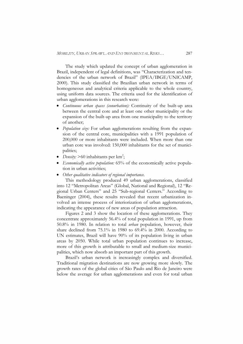
The study which updated the concept of urban agglomeration in Brazil, independent of legal definitions, was “Characterization and ten-dencies of the urban network of Brazil” (IPEA/IBGE/UNICAMP, 2000). This study classified the Brazilian urban network in terms of homogeneous and analytical criteria applicable to the whole country, using uniform data sources. The criteria used for the identification of urban agglomerations in this research were: Continuous urban spaces (conurbation): Continuity of the built-up area

between the central core and at least one other municipality or the expansion of the built-up area from one municipality to the territory of another;

Population size: For urban agglomerations resulting from the expan-sion of the central core, municipalities with a 1991 population of 200,000 or more inhabitants were included. When more than one urban core was involved: 150,000 inhabitants for the set of munici-palities;

Density: >60 inhabitants per km2; Economically active population: 65% of the economically active popula-

tion in urban activities; Other qualitative indicators of regional importance. This methodology produced 49 urban agglomerations, classified into 12 “Metropolitan Areas” (Global, National and Regional), 12 “Re-gional Urban Centers” and 25 “Sub-regional Centers.” According to Baeninger (2004), these results revealed that recent urbanization in-volved an intense process of interiorization of urban agglomerations, indicating the appearance of new areas of population attraction. Figures 2 and 3 show the location of these agglomerations. They concentrate approximately 56.4% of total population in 1991, up from 50.8% in 1980. In relation to total urban population, however, their share declined from 75.1% in 1980 to 69.4% in 2000. According to UN estimates, Brazil will have 90% of its population living in urban areas by 2050. While total urban population continues to increase, more of this growth is attributable to small and medium-size munici-palities, which now absorb an important part of this growth. Brazil’s urban network is increasingly complex and diversified. Traditional migration destinations are now growing more slowly. The growth rates of the global cities of São Paulo and Rio de Janeiro were below the average for urban agglomerations and even for total urban


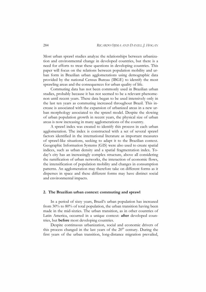
Figure 2 – Location of urban agglomerations in the North, Northeast and Central-West regions and in the States of Minas Gerais and Espírito Santo

Source: IBGE, Municipal digital shapes, 2000. population between 1980 and 1991; their share of total urban popula-tion declined from 42.8% in 1980 to 37% in 2000. These data require a better understanding of growth processes in this new spatial configura-tion. Once we recognize decentralization and de-concentration of the urban network, it is important to understand, in a comparative way, whether these processes are equally intense in all parts of the country, and especially whether spatial mobility has different impacts on urban form in different regions. Given this new configuration of the urban network, we then sought to determine the spatial distribution processes within the 49 agglomerations mentioned earlier. Our hypothesis is that these move-ments have now become an indispensable criterion for redefining met-ropolitan and regional limits, and that new intra-urban movements linked to dispersed and fragmented urbanization are especially impor-tant. These questions are raised at a moment of new growth tendencies of Brazilian cities. Recent migration is less similar to earlier rural-urban

State limits Urban agglomerations


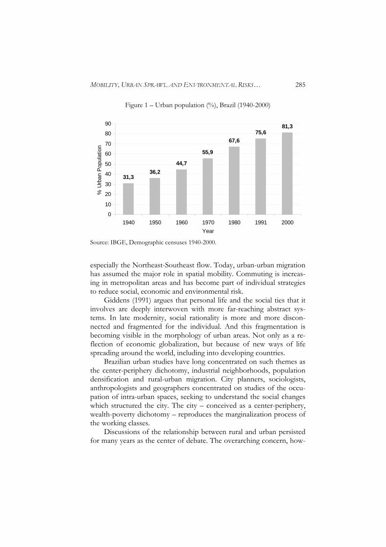
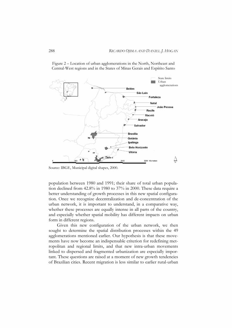
Figure 3 – Location of urban agglomerations in the South region and in the States of São Paulo and Rio de Janeiro

Source: IBGE, Municipal digital shapes, 2000. and long-distance migration, having shifted to a predominance of short-distance movements. Among the important types of this short-distance movement is the commuting pattern within metropolitan ar-eas, a type of urbanization more similar to sprawl-intense metropolises in other parts of the world. Commuting is an important condition for the consolidation of urban agglomerations. According to Hogan (1993), commuting plays an important role in sustainable development. While these movements may sometimes redi-rect the burden of environmental deterioration, favoring some groups and penalizing others, the possibility of carrying out diverse activities (residence, work, study, consumption) in different places serves to conciliate conflicting needs in individual households. On the one hand, there may be a tradeoff between new environmental stresses created by commuting and the attenuation of competing demands of household members. On the other hand, more complex mobility patterns may diminish the vulnerability of households to unemployment, to inade- quate educational or health services and to the isolation from family

State limits Urban agglomerations


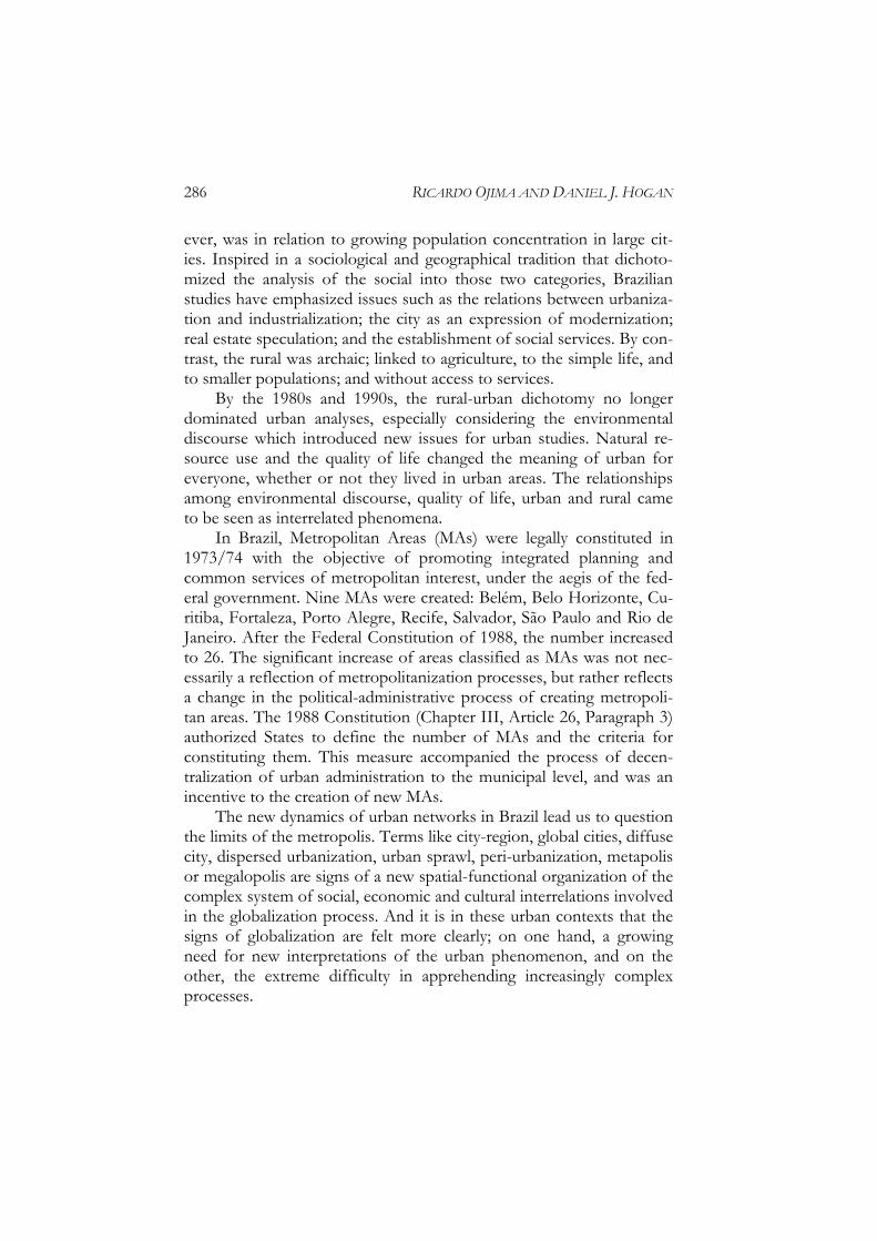
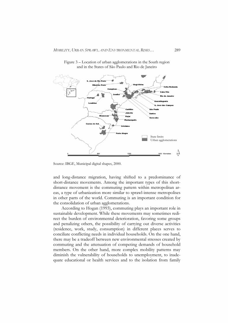
Figure 4 – Commuters by municipality of residence (2000)

State Limits

Number of daily commuters

1 dot = 100 persons

State Limits


1 dot = 100 persons

State Limits


1 dot = 100 persons

Source: IBGE, Demographic Census 2000.

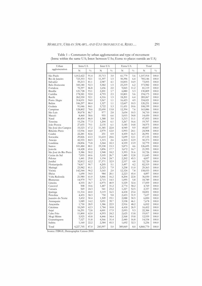
support which was often a result of earlier migration patterns. An examination of commuting data for the 49 urban agglomera-tions shows the relative concentration of this process. According to the 2000 Demographic Census, 7.4 million people worked or studied in municipalities other than that of residence, representing 4.4% of total population. The 49 urban agglomerations considered here account for more than 70% of those movements, 6.4% of the population of these areas. São Paulo and Rio de Janeiro concentrate 38% of all commuters. When we analyze those volumes in terms of proportion of total popu-lation, however, these cities give way to smaller places. In São Paulo and Rio de Janeiro commuters correspond to 6.6% and 7.4% of their total population, respectively, while in agglomerations such as Vitória (ES), Florianópolis (SC) and Jundiaí (SP), commuters represent more than 10% of total population. It is clear, then, that while commuting may be concentrated in some regions, it is not a phenomenon exclusive of traditional metropolises like São Paulo and Rio de Janeiro.


Table 1 – Commuters by urban agglomeration and type of movement (Intra: within the same UA; Inter: between UAs; Extra: to places outside an UA)

Intra UA Inter UA Extra UA Total Urban agglomeration N % N % N % N %

São Paulo 1,012,422 91.4 33,713 3.0 61,779 5.6 1,107,914 100.0 Rio de Janeiro 723,353 92.1 11,397 1.5 50,396 6.4 785,146 100.0 Salvador 59,213 81.1 2,987 4.1 10,855 14.9 73,055 100.0 Belo Horizonte 345,180 92.3 5,582 1.5 23,219 6.2 373,982 100.0 Fortaleza 70,397 86.8 1,656 2.0 9,065 11.2 81,119 100.0 Brasília 121,728 93.1 2,201 1.7 6,880 5.3 130,809 100.0 Curitiba 178,581 92.0 4,793 2.5 10,801 5.6 194,175 100.0 Recife 262,550 92.1 4,316 1.5 18,201 6.4 285,067 100.0 Porto Alegre 314,031 94.0 3,567 1.1 16,423 4.9 334,021 100.0 Belém 106,297 88.4 1,327 1.1 12,607 10.5 120,231 100.0 Goiânia 91,046 84.1 5,722 5.3 11,431 10.6 108,199 100.0 Campinas 128,802 78.6 22,690 13.8 12,394 7.6 163,886 100.0 São Luis 30,078 86.7 977 2.8 3,654 10.5 34,710 100.0 Maceió 8,460 58.6 955 6.6 5,015 34.8 14,430 100.0 Natal 40,454 86.0 1,388 3.0 5,213 11.1 47,055 100.0 Teresina 15,236 77.3 1,204 6.1 3,267 16.6 19,707 100.0 João Pessoa 27,655 79.1 2,135 6.1 5,185 14.8 34,975 100.0 São José dos Campos 33,523 67.2 11,385 22.8 4,949 9.9 49,857 100.0 Ribeirão Preto 15,936 64.0 2,979 12.0 5,993 24.1 24,908 100.0 Cuiabá 22,281 82.6 251 0.9 4,459 16.5 26,991 100.0 Sorocaba 29,826 63.3 11,610 24.6 5,699 12.1 47,135 100.0 Aracaju 42,555 84.5 1,315 2.6 6,503 12.9 50,373 100.0 Londrina 24,856 75.8 3,364 10.3 4,559 13.9 32,779 100.0 Santos 101,484 80.1 19,338 15.3 5,873 4.6 126,695 100.0 Joinvile 14,428 65.6 3,896 17.7 3,672 16.7 21,995 100.0 São José do Rio Preto 5,386 50.2 1,948 18.2 3,393 31.6 10,726 100.0 Caxias do Sul 7,055 60.6 3,105 26.7 1,485 12.8 11,645 100.0 Pelotas 1,441 29.8 1,194 24.7 2,202 45.5 4,837 100.0 Jundiaí 32,812 62.2 17,371 32.9 2,537 4.8 52,720 100.0 Florianópolis 74,817 90.7 4,205 5.1 3,497 4.2 82,519 100.0 Maringá 23,982 81.1 2,323 7.9 3,258 11.0 29,563 100.0 Vitória 142,544 90.2 3,165 2.0 12,324 7.8 158,033 100.0 Ilhéus 1,690 34.5 984 20.1 2,223 45.4 4,897 100.0 Volta Redonda 21,980 61.0 5,846 16.2 8,204 22.8 36,030 100.0 Blumenau 14,979 79.7 2,715 14.5 1,095 5.8 18,789 100.0 Limeira 4,555 26.7 6,975 40.9 5,529 32.4 17,059 100.0 Cascavel 508 10.6 1,487 31.2 2,774 58.2 4,769 100.0 Caruaru 569 24.3 541 23.2 1,227 52.5 2,337 100.0 Ipatinga 11,314 60.0 3,119 16.5 4,418 23.4 18,851 100.0 Petrolina 4,455 58.3 750 9.8 2,433 31.9 7,637 100.0 Juazeiro do Norte 3,452 50.4 1,309 19.1 2,088 30.5 6,850 100.0 Araraquara 1,089 14.2 3,051 39.7 3,538 46.1 7,678 100.0 Araçatuba 1,750 28.9 1,386 22.9 2,916 48.2 6,052 100.0 Criciúma 10,249 62.3 1,784 10.8 4,418 26.9 16,452 100.0 Itajaí 16,291 72.8 4,001 17.9 2,093 9.3 22,384 100.0 Cabo Frio 11,800 62.0 4,593 24.2 2,625 13.8 19,017 100.0 Mogi-Mirim 5,925 45.8 4,446 34.4 2,568 19.8 12,939 100.0 Guaratingueta 7,527 51.8 4,566 31.4 2,440 16.8 14,534 100.0 Itabira 1,160 22.2 2,384 45.5 1,692 32.3 5,236 100.0

Total 4,227,705 87.0 243,997 5.0 389,069 8.0 4,860,770 100.0

Source: FIBGE, Demographic Census 2000.


As a result of the increase of commuting in Brazil, urban areas look more and more like classic sprawl. While the term “urban sprawl” emerged around 1960 as a pejorative designation to express the uncon-trolled expansion of North American urban areas, above all in refer-ence to the suburban pattern of urbanization (Kiefer, 2003), it refers basically to a pattern of low density. Although the definition of the term is still controversial, there is a considerable body of research which shows the importance of the phenomenon in other areas of the world, mostly on the basis of case studies. Los Angeles is one of the most cited cases. Between 1970 and 1990, the population of the Los Angeles area grew by 45%, while the physical area occupied by this population grew by 300% (Meadows, 1999); in other words, there was a significant reduction in urban den-sity. Outlying areas grew at the expense of the consolidated urban cen-ter. In general, the consensus on the sprawl debate is this gap between population growth and the physical expansion of the city, which ex-plains the tendency toward low urban densities in most metropolitan areas of the world. In this sense, several studies show the same urban distortion of Los Angeles occurring in several areas of the United States and in other areas of the world. Even in European cities, tradi-tionally associated with a compact urban form (Richardson and Chang-Hee, 2004), there are signs that sprawl is increasing. Urban sprawl research leans heavily on case studies. They demon-strate the historical processes of urban occupation and how urban lim-its changed over time. However, from an historical point of view, urban growth associated to physical expansion is not a new concern; to a certain extent, growth has always meant territorial expansion. What is new today is the fact that new urban forms have appeared over the second half of the 20th century. According to Richardson and Chang-Hee (2004:1), there seems to be a convergence in urban settlement pat-terns in the United States and Western Europe. This transition can be observed in lifestyles which are dissemi-nated through large urban centers, propelled by the globalization of consumption patterns, which produce increasing homogeneity in dif-ferent areas of the world. Dependence on individual transportation plays an important role in the compression of space and time in post-modern cities. As part of this process, both medium and long-distance commuting is becoming much more evident.


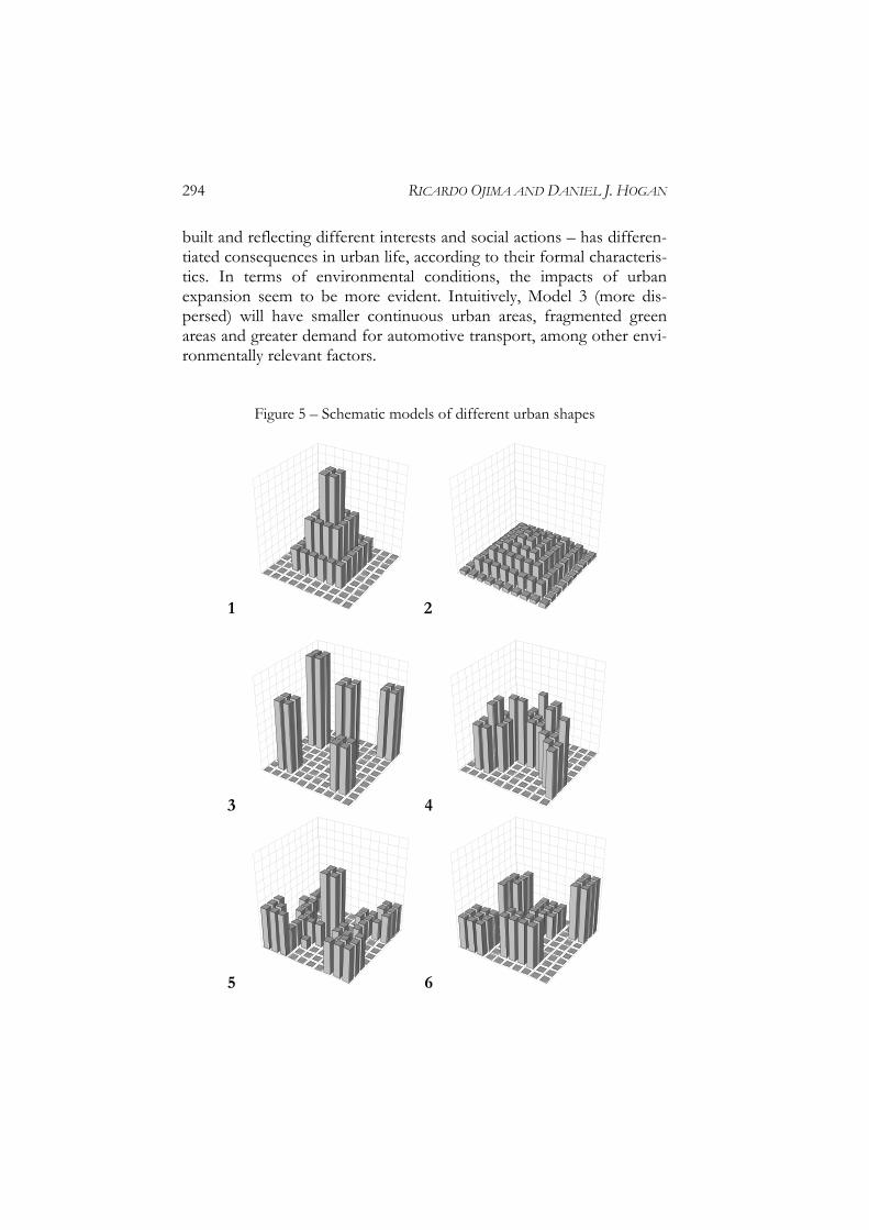
But what is sprawl in the context of developing countries? It is clear that the drivers of sprawl are not the same in different social con-texts, even considering the homogenization of consumption patterns in the world’s cities. In Brazil, mega-cities like São Paulo and Rio de Ja-neiro reveal a certain ambiguity in this regard, and new social behaviors are not so directly reflected in these cities’ consolidated urban form. In the case of newer metropolitan areas like Brasilia or Campinas, the morphological consequences of new behaviors can be more easily ob-served. It is important to keep in mind, then, that Brazilian urbaniza-tion is not explained only by the experience of São Paulo or Rio de Janeiro, in spite of their population concentration. Urbanization is in-creasingly characterized by a complex network of urban areas in the country as a whole. 3. Data and method: measuring sprawl in Brazil The challenge of studying the dimensions of urban sprawl may be summarized as the task of measuring the urban expansion which ex-trapolates the limits of a conurbation. The urban sprawl literature seeks to identify empirically observable factors in metropolitan areas, in or-der to compare a country’s overall situation. In the present study, then, urban sprawl is understood as a process and not as a phenomenon in itself, since the empirical phenomenon can only be apprehended in comparative terms. To elucidate this relationship, in an effort to generalize, we can hypothesize different forms of urban settlement and assess their im-pact on urban life. Figure 5 shows how a population’s distribution in the intra-urban space can assume different expressions in spite of the same average density. Models 1 and 2 represent typical monocentric cities, but with dif-ferent spatial distributions, the first being more compact. Model 3 is clearly more fragmented and, as is also the case of Model 2, can be classified as more dispersed than Model 1. While Models 4, 5 and 6 seem to be more similar, Model 4 possesses more pronounced conti-nuity than Models 5 and 6. If those models represent urban areas or urban agglomerations, what could be said in this respect? Do people who live in two different areas, for example, in Models 1 and 5, have similar daily activities? The hypothesis is that urban space – socially


built and reflecting different interests and social actions – has differen-tiated consequences in urban life, according to their formal characteris-tics. In terms of environmental conditions, the impacts of urban expansion seem to be more evident. Intuitively, Model 3 (more dis-persed) will have smaller continuous urban areas, fragmented green areas and greater demand for automotive transport, among other envi-ronmentally relevant factors.

Figure 5 – Schematic models of different urban shapes

1 2

3 4

5 6


Of course it is not possible to summarize the complexity of ur-banization with such simplified schematic models, using a classification based on single-factor categories, but it is unquestionable that Brazilian urban agglomerations take on very different formal dimensions. In terms of the perception of the person who travels from one city to an-other, it is common to hear comparisons between origin and destina-tion city to the effect that distances between one activity and another are greater, that spatial organization is different, or that traffic jams and access to services are worse. The objective of this section, then, is to identify, from the sprawl literature, the principal indicators for classifying an urban area in terms of urban dispersion. These dimensions are then applied to 37 selected urban agglomerations to obtain a ranking of urban sprawl and to map sprawling situations in the country. The selection of 37 of the 49 urban agglomerations was based on the results presented in Table 1, consid-ering those agglomerations with predominantly intra-UA commuters. Additionally, we excluded urban agglomerations composed of only two municipalities (UA of Teresina, Cuiabá and Petrolina/Juazeiro) even when they show important intra-UA commuting. The index is presented in the next section in Table 6, which sum-marizes the dimensions considered for the Brazilian sprawl index. Fi-nally, the section seeks to verify the existence, or not, of a “pattern” in contemporary Brazilian urbanization and whether this “pattern” can be apprehended in spatial terms in a comparative way, in a diversity of economic, social, political and demographic contexts. 3.1. Density The works of Galster et al. (2001), Batty et al. (1999), Chin (2002), Torrens and Alberti (2000), Cutsinger et al. (2005), Roca et al. (2004), Angel et al. (2005), among others, used satellite images to evaluate ur-ban expansion in several parts of the world. Angel et al. present a worldwide study considering a group of approximately 4 thousand cit-ies with population greater than 100 thousand inhabitants. In this study, the densities of developing country cities tend to be greater than in the developed countries; however, in both groups the tendency over time has been toward lower density. The Global Rural-Urban Mapping Project (GRUMP) developed at the Center for International Earth Science Information Network (CI-


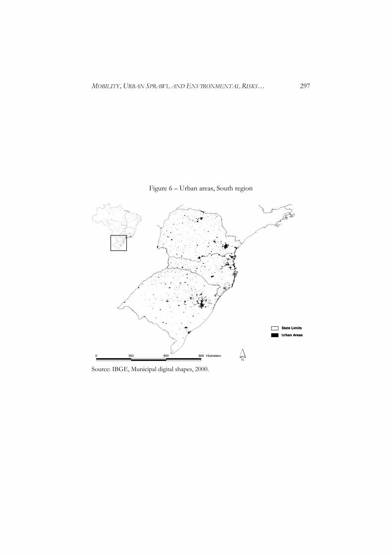
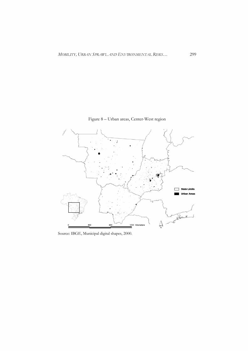
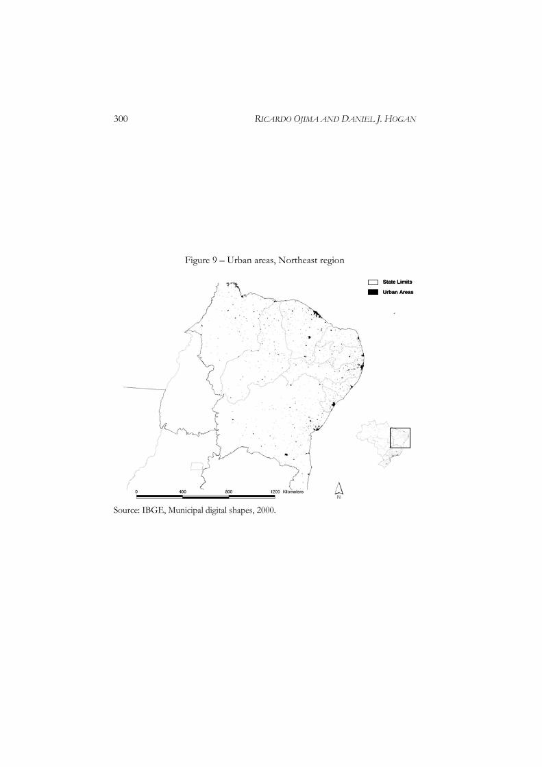
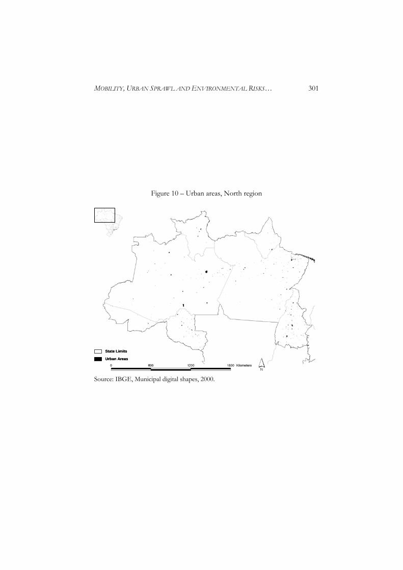
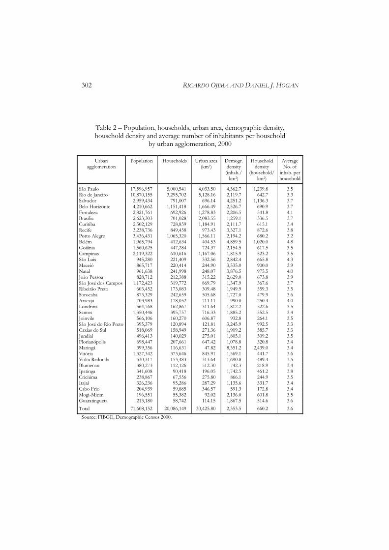
ESIN), Columbia University, used satellite images and nighttime lights emitted by urban agglomerations to estimate urbanized areas. And in Brazil, Kampel (2003) has carried out similar work in the Amazonian State of Pará. But the systematic use of these instruments still has operational limitations. Among them is the high cost of acquiring the images and the subsequent processing and analysis, above all when more detailed spatial units are needed, as in the case of urban agglomerations which are not part of institutionalized metropolitan areas in Brazil. For these reasons, official IBGE data on urban and rural census tracts were used; these are public access data, available in digital for-mat. Garcia and Matos (2005) also used these data and discussed their under-utilization in Brazilian urban studies. These data are organized in a Geographical Information System and classify census tracts into ur-ban/rural categories, detailing each situation according to function. For example, it distinguishes areas with rural villages from those areas of agricultural use only. The total urban area in Brazil, according to this criterion, is ap-proximately 95 thousand km2, which represents 1.12% of Brazilian ter-ritory, holding 140 million people – 81.8% of total population in 2000. This reduced share of national territory occupied by cities is visualized in Figures 6 to 10; Southeast and South regions have the largest urban areas. The national population density is approximately 20 inhabitants per km2; when only the urban area is considered, density is 1,400 in-habitants per km2. The selected 37 urban agglomerations represent about 1/3 of the total urban area (30.5 thousand km2) and concentrate 71.6 million people. Population density in these agglomerations is 2,353 inhabitants per km2. The region with the highest urban density has 8,300 inhabitants per km2 and the lowest density is 600 inhabitants per km2. Very different situations exist, then, in terms of urban density. São Paulo, for example, in spite of holding second place in terms of territorial size (with 4,000 km2), has one of the highest urban densities (4.3 thousand inhabitants per km2).


Figure 6 – Urban areas, South region

Source: IBGE, Municipal digital shapes, 2000.

State Limits

Urban Areas

State Limits

Urban Areas


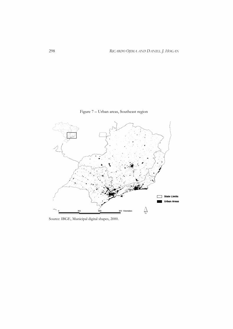
Figure 7 – Urban areas, Southeast region


State Limits

Urban Areas

State Limits

Urban Areas


Figure 8 – Urban areas, Center-West region


State Limits

Urban Areas

State Limits

Urban Areas


Figure 9 – Urban areas, Northeast region


State Limits

Urban Areas

State Limits

Urban Areas


Figure 10 – Urban areas, North region


State Limits

Urban Areas

State Limits

Urban Areas


Table 2 – Population, households, urban area, demographic density, household density and average number of inhabitants per household

by urban agglomeration, 2000

Urban agglomeration

Population Households Urban area (km2)

Demogr. density (inhab./

km2)

Household density

(household/km2)

Average No. of

inhab. per household

São Paulo 17,596,957 5,000,541 4,033.50 4,362.7 1,239.8 3.5 Rio de Janeiro 10,870,155 3,295,702 5,128.16 2,119.7 642.7 3.3 Salvador 2,959,434 791,007 696.14 4,251.2 1,136.3 3.7 Belo Horizonte 4,210,662 1,151,418 1,666.49 2,526.7 690.9 3.7 Fortaleza 2,821,761 692,926 1,278.83 2,206.5 541.8 4.1 Brasília 2,623,303 701,028 2,083.55 1,259.1 336.5 3.7 Curitiba 2,502,129 728,859 1,184.91 2,111.7 615.1 3.4 Recife 3,238,736 849,458 973.43 3,327.1 872.6 3.8 Porto Alegre 3,436,431 1,065,320 1,566.11 2,194.2 680.2 3.2 Belém 1,965,794 412,634 404.53 4,859.5 1,020.0 4.8 Goiânia 1,560,625 447,284 724.37 2,154.5 617.5 3.5 Campinas 2,119,322 610,616 1,167.06 1,815.9 523.2 3.5 São Luis 945,280 221,409 332.56 2,842.4 665.8 4.3 Maceió 865,717 220,414 244.90 3,535.0 900.0 3.9 Natal 961,638 241,998 248.07 3,876.5 975.5 4.0 João Pessoa 828,712 212,388 315.22 2,629.0 673.8 3.9 São José dos Campos 1,172,423 319,772 869.79 1,347.9 367.6 3.7 Ribeirão Preto 603,452 173,083 309.48 1,949.9 559.3 3.5 Sorocaba 873,329 242,659 505.68 1,727.0 479.9 3.6 Aracaju 703,983 178,052 711.11 990.0 250.4 4.0 Londrina 564,768 162,867 311.64 1,812.2 522.6 3.5 Santos 1,350,446 395,757 716.33 1,885.2 552.5 3.4 Joinvile 566,106 160,270 606.87 932.8 264.1 3.5 São José do Rio Preto 395,379 120,894 121.81 3,245.9 992.5 3.3 Caxias do Sul 518,069 158,949 271.36 1,909.2 585.7 3.3 Jundiaí 496,413 140,029 275.01 1,805.1 509.2 3.5 Florianópolis 698,447 207,661 647.42 1,078.8 320.8 3.4 Maringá 399,356 116,631 47.82 8,351.2 2,439.0 3.4 Vitória 1,327,342 373,646 845.91 1,569.1 441.7 3.6 Volta Redonda 530,317 153,483 313.64 1,690.8 489.4 3.5 Blumenau 380,273 112,126 512.30 742.3 218.9 3.4 Ipatinga 341,608 90,418 196.05 1,742.5 461.2 3.8 Criciúma 238,867 67,556 275.80 866.1 244.9 3.5 Itajaí 326,236 95,286 287.29 1,135.6 331.7 3.4 Cabo Frio 204,939 59,885 346.57 591.3 172.8 3.4 Mogi-Mirim 196,551 55,382 92.02 2,136.0 601.8 3.5 Guaratingueta 213,180 58,742 114.15 1,867.5 514.6 3.6

Total 71,608,152 20,086,149 30,425.80 2,353.5 660.2 3.6



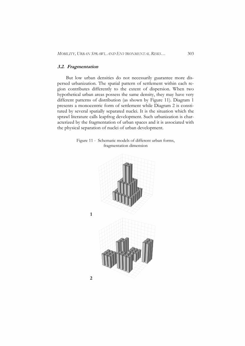
3.2. Fragmentation But low urban densities do not necessarily guarantee more dis-persed urbanization. The spatial pattern of settlement within each re-gion contributes differently to the extent of dispersion. When two hypothetical urban areas possess the same density, they may have very different patterns of distribution (as shown by Figure 11). Diagram 1 presents a monocentric form of settlement while Diagram 2 is consti-tuted by several spatially separated nuclei. It is the situation which the sprawl literature calls leapfrog development. Such urbanization is char-acterized by the fragmentation of urban spaces and it is associated with the physical separation of nuclei of urban development.

Figure 11 - Schematic models of different urban forms,

fragmentation dimension

1

2


Leapfrog development can be understood as part of an unconnected-ness of daily life spaces within the urban agglomeration and it is clearly associated to changes in the spatial displacements of population, given that the continuity of the urban area is no longer necessary for its inte-gration. This aspect of urban development is, after density, the most characteristic factor of urban sprawl, because it provides spatial evi-dence of the pattern of population distribution of urban areas. In op-erational terms, the fragmentation of urban spaces can be apprehended in different ways. As we can observe in an intuitive way from Figure 11, distance between urbanized areas is a measure of dispersion. In other words, two areas with the same population, distributed in an equivalent urban area, may have similar densities; but one may have a compact form of concentric circles while the other may be polycentric, with urban branches going in different directions. Urbanization by leaps may compromise agricultural uses in outly-ing areas and also require expansion of the network of infrastructure services – water supply and sewage collection (Angel et al., 2005). Envi-ronment is an important aspect for this dimension, because both causes and effects may be identified. On the one hand, there is a grow-ing demand for environmental amenities in residential areas. On the other hand, as urban growth reaches these areas, such amenities are compromised. The trend, then, is the creation of urban spaces more and more disconnected from each other. To measure this dimension, the Average Nearest Neighbor Index was used, using the software Arc-Gis (version 9.0).

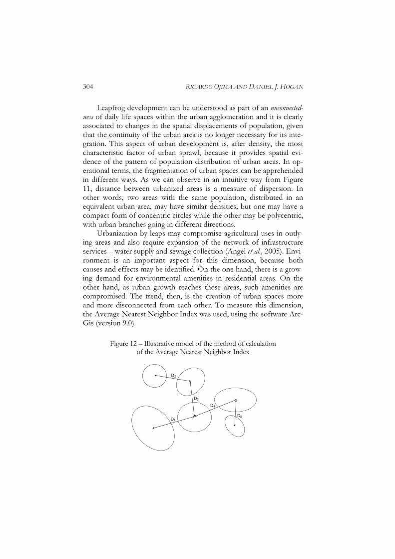
Figure 12 – Illustrative model of the method of calculation

of the Average Nearest Neighbor Index

D1

D2

D3

D4

D5


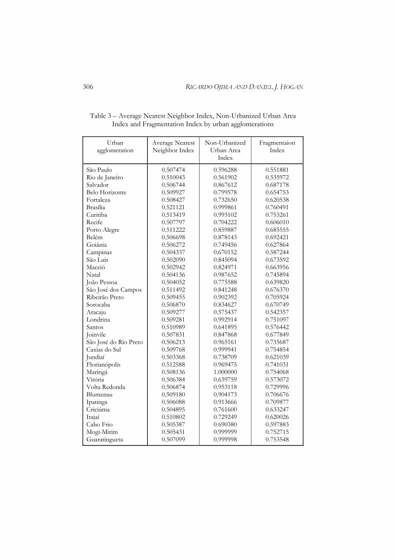
This index measures the distances between polygons defined by their contiguous urban census tracts and their respective standard de-viations for each study area. The ratio between the average of those distances and the average of the distances in a hypothetical area with random distribution is an indicator that allows us to measure the de-gree of dispersion of the urbanized areas in each of the agglomerations. That indicator was later adjusted so that values varied between zero and one. Values closer to zero represent more compact patterns while values closer to one, the most dispersed patterns. The same procedure was carried out for each of the 37 selected areas. Also using the pro-portion of non-urbanized areas2 of the agglomerations, an arithmetic average was calculated of both indices to compose a Fragmentation Index, as shown in Table 3. 3.3. Orientation/Linearity The geographic orientation of cities also plays an important role in urban expansion and in the amount of sprawl. The growth of some urban agglomerations is conditioned by physical constraints such as mountains, rivers, oceans or other natural barriers. They may also have a direct relationship with other elements such as highways, railroads and regional economic poles. Under such conditions, urban areas grow in different ways, which should be taken into account when urban form is analyzed. An urban agglomeration that grows on the basis of concentric circles potentially has a greater capacity to optimize the distribution of service infrastruc-ture compared to a region that develops following a highway, for in-stance. It is important to differentiate areas in terms of the orientation of their expansion; in other words, whether the form is more circular or more ellipsoidal. Referring again to the diagrams of hypothetical ar-eas (Figure 13), we can observe two areas with the same density and little fragmentation. However, the pattern of urban development in Model 2 is linear and tends toward more sprawl, as we can see intui-tively in Diagrams 1 and 2.

―――― 2. Defined by the Census Bureau as non-urbanized areas inside the urban perime-ter.


Table 3 – Average Nearest Neighbor Index, Non-Urbanized Urban Area

Index and Fragmentation Index by urban agglomerations

Urban agglomeration

Average Nearest Neighbor Index

Non-Urbanized Urban Area

Index

Fragmentaion Index

São Paulo 0.507474 0.596288 0.551881 Rio de Janeiro 0.510043 0.561902 0.535972 Salvador 0.506744 0.867612 0.687178 Belo Horizonte 0.509927 0.799578 0.654753 Fortaleza 0.508427 0.732650 0.620538 Brasília 0.521121 0.999861 0.760491 Curitiba 0.513419 0.993102 0.753261 Recife 0.507797 0.704222 0.606010 Porto Alegre 0.511222 0.859887 0.685555 Belém 0.506698 0.878143 0.692421 Goiânia 0.506272 0.749456 0.627864 Campinas 0.504337 0.670152 0.587244 São Luis 0.502090 0.845094 0.673592 Maceió 0.502942 0.824971 0.663956 Natal 0.504136 0.987652 0.745894 João Pessoa 0.504052 0.775588 0.639820 São José dos Campos 0.511492 0.841248 0.676370 Ribeirão Preto 0.509455 0.902392 0.705924 Sorocaba 0.506870 0.834627 0.670749 Aracaju 0.509277 0.575437 0.542357 Londrina 0.509281 0.992914 0.751097 Santos 0.510989 0.641895 0.576442 Joinvile 0.507831 0.847868 0.677849 São José do Rio Preto 0.506213 0.965161 0.735687 Caxias do Sul 0.509768 0.999941 0.754854 Jundiaí 0.503368 0.738709 0.621039 Florianópolis 0.512588 0.969475 0.741031 Maringá 0.508136 1.000000 0.754068 Vitória 0.506384 0.639759 0.573072 Volta Redonda 0.506874 0.953118 0.729996 Blumenau 0.509180 0.904173 0.706676 Ipatinga 0.506088 0.913666 0.709877 Criciúma 0.504895 0.761600 0.633247 Itajaí 0.510802 0.729249 0.620026 Cabo Frio 0.505387 0.690380 0.597883 Mogi-Mirim 0.505431 0.999999 0.752715 Guaratingueta 0.507099 0.999998 0.753548


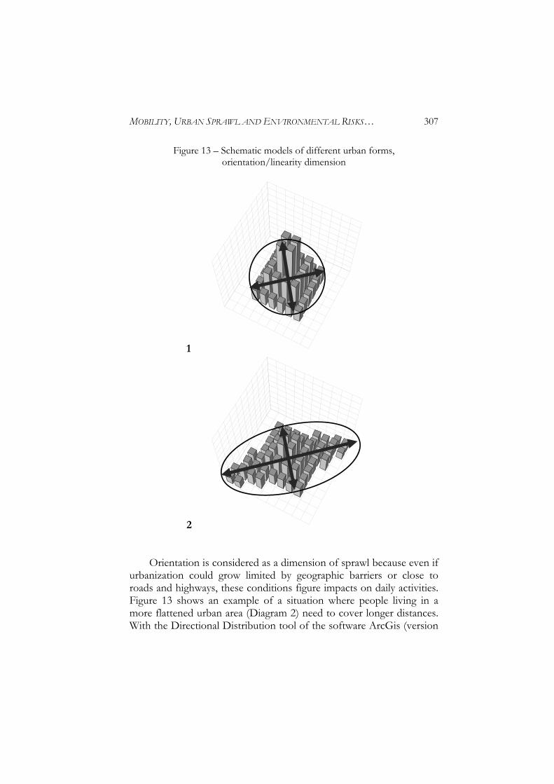
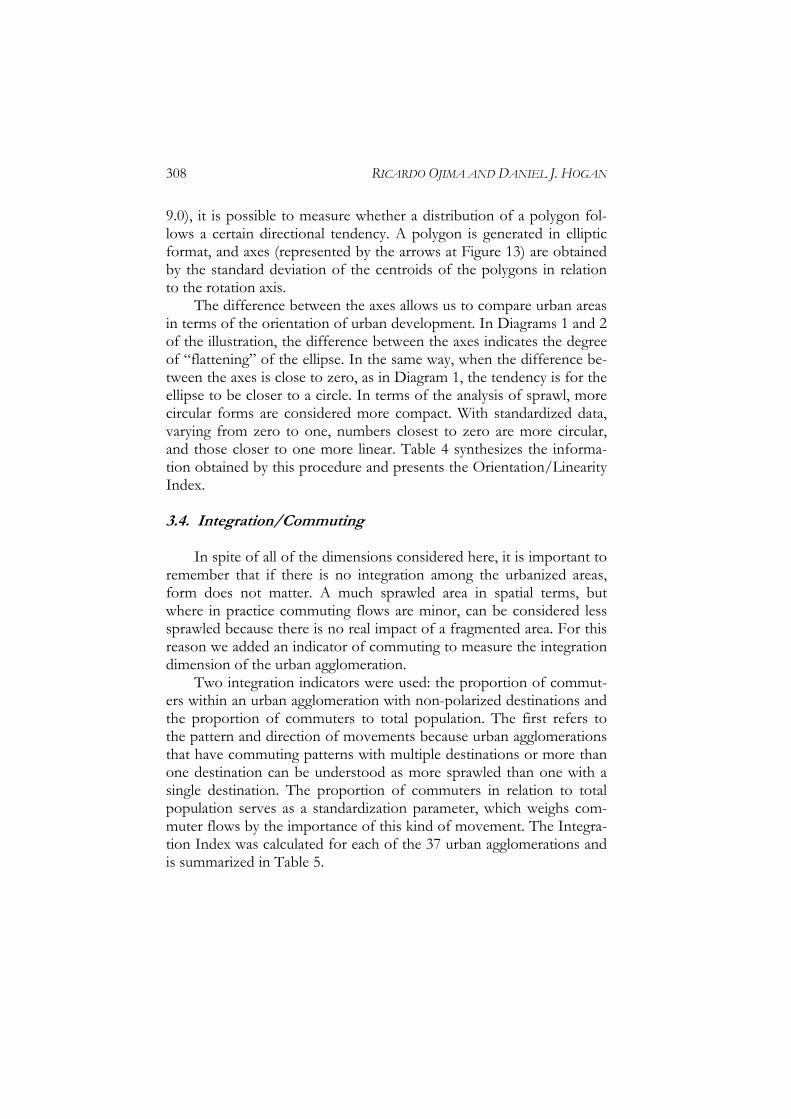
Figure 13 – Schematic models of different urban forms, orientation/linearity dimension

1

2 Orientation is considered as a dimension of sprawl because even if urbanization could grow limited by geographic barriers or close to roads and highways, these conditions figure impacts on daily activities. Figure 13 shows an example of a situation where people living in a more flattened urban area (Diagram 2) need to cover longer distances. With the Directional Distribution tool of the software ArcGis (version


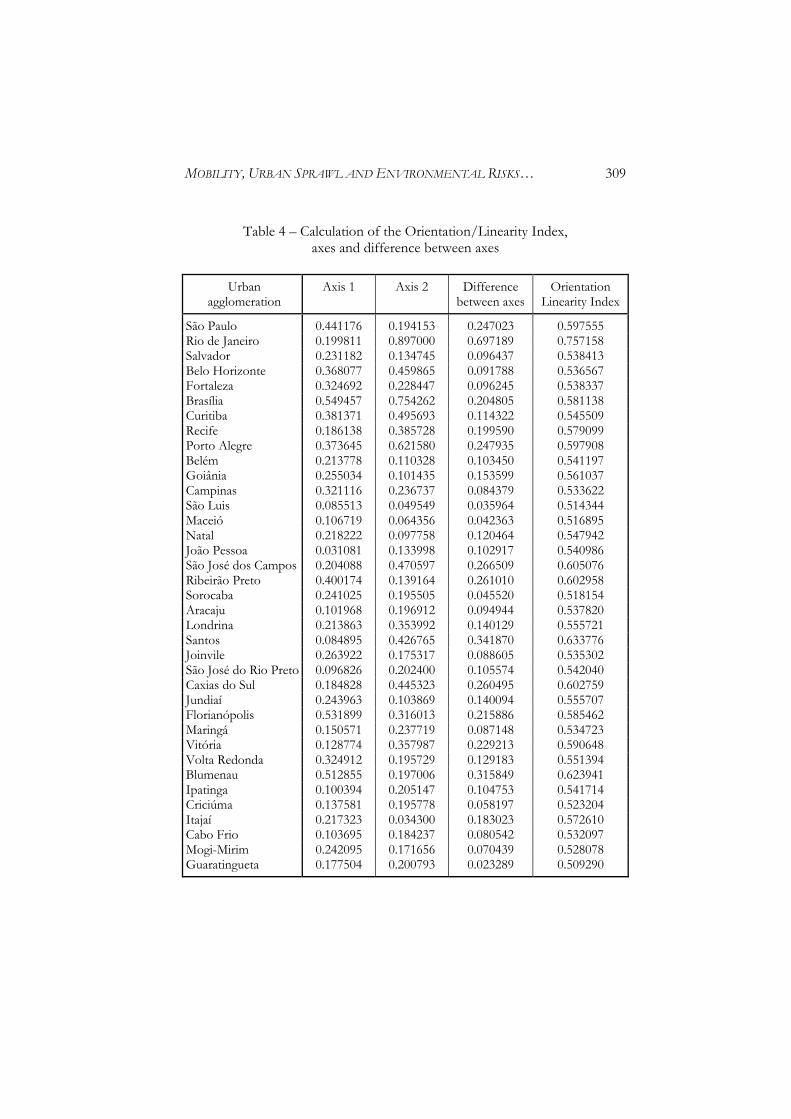
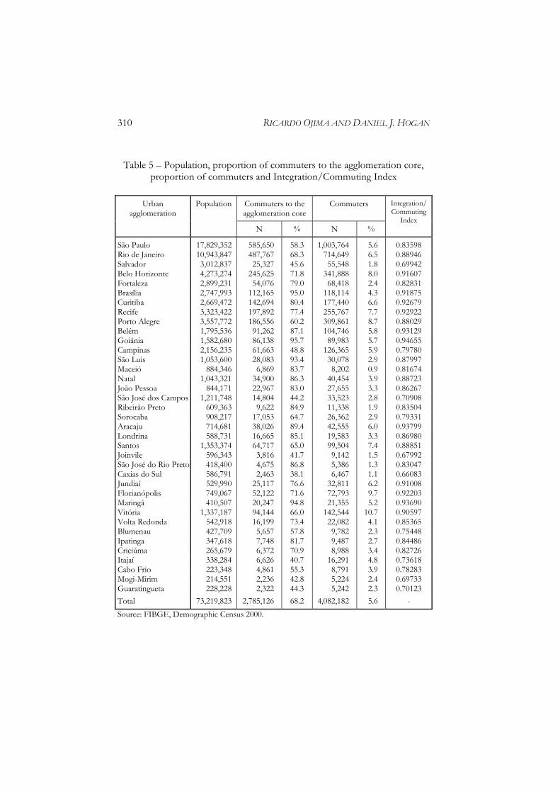
9.0), it is possible to measure whether a distribution of a polygon fol-lows a certain directional tendency. A polygon is generated in elliptic format, and axes (represented by the arrows at Figure 13) are obtained by the standard deviation of the centroids of the polygons in relation to the rotation axis. The difference between the axes allows us to compare urban areas in terms of the orientation of urban development. In Diagrams 1 and 2 of the illustration, the difference between the axes indicates the degree of “flattening” of the ellipse. In the same way, when the difference be-tween the axes is close to zero, as in Diagram 1, the tendency is for the ellipse to be closer to a circle. In terms of the analysis of sprawl, more circular forms are considered more compact. With standardized data, varying from zero to one, numbers closest to zero are more circular, and those closer to one more linear. Table 4 synthesizes the informa-tion obtained by this procedure and presents the Orientation/Linearity Index. 3.4. Integration/Commuting In spite of all of the dimensions considered here, it is important to remember that if there is no integration among the urbanized areas, form does not matter. A much sprawled area in spatial terms, but where in practice commuting flows are minor, can be considered less sprawled because there is no real impact of a fragmented area. For this reason we added an indicator of commuting to measure the integration dimension of the urban agglomeration. Two integration indicators were used: the proportion of commut-ers within an urban agglomeration with non-polarized destinations and the proportion of commuters to total population. The first refers to the pattern and direction of movements because urban agglomerations that have commuting patterns with multiple destinations or more than one destination can be understood as more sprawled than one with a single destination. The proportion of commuters in relation to total population serves as a standardization parameter, which weighs com-muter flows by the importance of this kind of movement. The Integra-tion Index was calculated for each of the 37 urban agglomerations and is summarized in Table 5.


Table 4 – Calculation of the Orientation/Linearity Index,

axes and difference between axes

Urban agglomeration

Axis 1 Axis 2 Difference between axes

Orientation Linearity Index

São Paulo 0.441176 0.194153 0.247023 0.597555 Rio de Janeiro 0.199811 0.897000 0.697189 0.757158 Salvador 0.231182 0.134745 0.096437 0.538413 Belo Horizonte 0.368077 0.459865 0.091788 0.536567 Fortaleza 0.324692 0.228447 0.096245 0.538337 Brasília 0.549457 0.754262 0.204805 0.581138 Curitiba 0.381371 0.495693 0.114322 0.545509 Recife 0.186138 0.385728 0.199590 0.579099 Porto Alegre 0.373645 0.621580 0.247935 0.597908 Belém 0.213778 0.110328 0.103450 0.541197 Goiânia 0.255034 0.101435 0.153599 0.561037 Campinas 0.321116 0.236737 0.084379 0.533622 São Luis 0.085513 0.049549 0.035964 0.514344 Maceió 0.106719 0.064356 0.042363 0.516895 Natal 0.218222 0.097758 0.120464 0.547942 João Pessoa 0.031081 0.133998 0.102917 0.540986 São José dos Campos 0.204088 0.470597 0.266509 0.605076 Ribeirão Preto 0.400174 0.139164 0.261010 0.602958 Sorocaba 0.241025 0.195505 0.045520 0.518154 Aracaju 0.101968 0.196912 0.094944 0.537820 Londrina 0.213863 0.353992 0.140129 0.555721 Santos 0.084895 0.426765 0.341870 0.633776 Joinvile 0.263922 0.175317 0.088605 0.535302 São José do Rio Preto 0.096826 0.202400 0.105574 0.542040 Caxias do Sul 0.184828 0.445323 0.260495 0.602759 Jundiaí 0.243963 0.103869 0.140094 0.555707 Florianópolis 0.531899 0.316013 0.215886 0.585462 Maringá 0.150571 0.237719 0.087148 0.534723 Vitória 0.128774 0.357987 0.229213 0.590648 Volta Redonda 0.324912 0.195729 0.129183 0.551394 Blumenau 0.512855 0.197006 0.315849 0.623941 Ipatinga 0.100394 0.205147 0.104753 0.541714 Criciúma 0.137581 0.195778 0.058197 0.523204 Itajaí 0.217323 0.034300 0.183023 0.572610 Cabo Frio 0.103695 0.184237 0.080542 0.532097 Mogi-Mirim 0.242095 0.171656 0.070439 0.528078 Guaratingueta 0.177504 0.200793 0.023289 0.509290


Table 5 – Population, proportion of commuters to the agglomeration core,

proportion of commuters and Integration/Commuting Index

Commuters to the agglomeration core

Commuters Urban agglomeration

Population

N % N %

Integration/ Commuting

Index

São Paulo 17,829,352 585,650 58.3 1,003,764 5.6 0.83598 Rio de Janeiro 10,943,847 487,767 68.3 714,649 6.5 0.88946 Salvador 3,012,837 25,327 45.6 55,548 1.8 0.69942 Belo Horizonte 4,273,274 245,625 71.8 341,888 8.0 0.91607 Fortaleza 2,899,231 54,076 79.0 68,418 2.4 0.82831 Brasília 2,747,993 112,165 95.0 118,114 4.3 0.91875 Curitiba 2,669,472 142,694 80.4 177,440 6.6 0.92679 Recife 3,323,422 197,892 77.4 255,767 7.7 0.92922 Porto Alegre 3,557,772 186,556 60.2 309,861 8.7 0.88029 Belém 1,795,536 91,262 87.1 104,746 5.8 0.93129 Goiânia 1,582,680 86,138 95.7 89,983 5.7 0.94655 Campinas 2,156,235 61,663 48.8 126,365 5.9 0.79780 São Luis 1,053,600 28,083 93.4 30,078 2.9 0.87997 Maceió 884,346 6,869 83.7 8,202 0.9 0.81674 Natal 1,043,321 34,900 86.3 40,454 3.9 0.88723 João Pessoa 844,171 22,967 83.0 27,655 3.3 0.86267 São José dos Campos 1,211,748 14,804 44.2 33,523 2.8 0.70908 Ribeirão Preto 609,363 9,622 84.9 11,338 1.9 0.83504 Sorocaba 908,217 17,053 64.7 26,362 2.9 0.79331 Aracaju 714,681 38,026 89.4 42,555 6.0 0.93799 Londrina 588,731 16,665 85.1 19,583 3.3 0.86980 Santos 1,353,374 64,717 65.0 99,504 7.4 0.88851 Joinvile 596,343 3,816 41.7 9,142 1.5 0.67992 São José do Rio Preto 418,400 4,675 86.8 5,386 1.3 0.83047 Caxias do Sul 586,791 2,463 38.1 6,467 1.1 0.66083 Jundiaí 529,990 25,117 76.6 32,811 6.2 0.91008 Florianópolis 749,067 52,122 71.6 72,793 9.7 0.92203 Maringá 410,507 20,247 94.8 21,355 5.2 0.93690 Vitória 1,337,187 94,144 66.0 142,544 10.7 0.90597 Volta Redonda 542,918 16,199 73.4 22,082 4.1 0.85365 Blumenau 427,709 5,657 57.8 9,782 2.3 0.75448 Ipatinga 347,618 7,748 81.7 9,487 2.7 0.84486 Criciúma 265,679 6,372 70.9 8,988 3.4 0.82726 Itajaí 338,284 6,626 40.7 16,291 4.8 0.73618 Cabo Frio 223,348 4,861 55.3 8,791 3.9 0.78283 Mogi-Mirim 214,551 2,236 42.8 5,224 2.4 0.69733 Guaratingueta 228,228 2,322 44.3 5,242 2.3 0.70123

Total 73,219,823 2,785,126 68.2 4,082,182 5.6 -



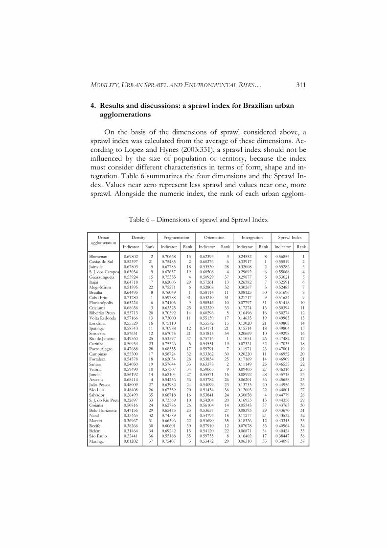
4. Results and discussions: a sprawl index for Brazilian urban agglomerations

On the basis of the dimensions of sprawl considered above, a sprawl index was calculated from the average of these dimensions. Ac-cording to Lopez and Hynes (2003:331), a sprawl index should not be influenced by the size of population or territory, because the index must consider different characteristics in terms of form, shape and in-tegration. Table 6 summarizes the four dimensions and the Sprawl In-dex. Values near zero represent less sprawl and values near one, more sprawl. Alongside the numeric index, the rank of each urban agglom-

Table 6 – Dimensions of sprawl and Sprawl Index

Density Fragmentation Orientation Intergration Sprawl Index Urban agglomeration

Indicator Rank Indicator Rank Indicator Rank Indicator Rank Indicator Rank

Blumenau 0.69802 2 0.70668 13 0.62394 3 0.24552 8 0.56854 1 Caxias do Sul 0.52397 21 0.75485 2 0.60276 6 0.33917 1 0.55519 2 Joinvile 0.67803 5 0.67785 18 0.53530 28 0.32008 2 0.55282 3 S. J. dos Campos 0.63034 9 0.67637 19 0.60508 4 0.29092 6 0.55068 4 Guaratingueta 0.55924 15 0.75355 4 0.50929 37 0.29877 5 0.53021 5 Itajaí 0.64718 7 0.62003 29 0.57261 13 0.26382 7 0.52591 6 Mogi-Mirim 0.51595 22 0.75271 6 0.52808 32 0.30267 3 0.52485 7 Brasília 0.64495 8 0.76049 1 0.58114 11 0.08125 30 0.51696 8 Cabo Frio 0.71780 1 0.59788 31 0.53210 31 0.21717 9 0.51624 9 Florianópolis 0.65224 6 0.74103 9 0.58546 10 0.07797 31 0.51418 10 Criciúma 0.68656 3 0.63325 25 0.52320 33 0.17274 13 0.50394 11 Ribeirão Preto 0.53713 20 0.70592 14 0.60296 5 0.16496 16 0.50274 12 Volta Redonda 0.57166 13 0.73000 11 0.55139 17 0.14635 19 0.49985 13 Londrina 0.55529 16 0.75110 7 0.55572 15 0.13020 21 0.49808 14 Ipatinga 0.58543 11 0.70988 12 0.54171 21 0.15514 18 0.49804 15 Sorocaba 0.57631 12 0.67075 21 0.51815 34 0.20669 10 0.49298 16 Rio de Janeiro 0.49560 25 0.53597 37 0.75716 1 0.11054 26 0.47482 17 Curitiba 0.50934 23 0.75326 5 0.54551 19 0.07321 32 0.47033 18 Porto Alegre 0.47688 28 0.68555 17 0.59791 7 0.11971 23 0.47001 19 Campinas 0.55500 17 0.58724 32 0.53362 30 0.20220 11 0.46952 20 Fortaleza 0.54578 18 0.62054 28 0.53834 25 0.17169 14 0.46909 21 Santos 0.54050 19 0.57644 33 0.63378 2 0.11149 25 0.46555 22 Vitória 0.59490 10 0.57307 34 0.59065 9 0.09403 27 0.46316 23 Jundiaí 0.56192 14 0.62104 27 0.55571 16 0.08992 28 0.45715 24 Aracaju 0.68414 4 0.54236 36 0.53782 26 0.06201 36 0.45658 25 João Pessoa 0.48009 27 0.63982 24 0.54099 23 0.13733 20 0.44956 26 São Luis 0.48408 26 0.67359 20 0.51434 36 0.12003 22 0.44801 27 Salvador 0.26499 35 0.68718 16 0.53841 24 0.30058 4 0.44779 28 S. J. do Rio Preto 0.32697 33 0.73569 10 0.54204 20 0.16953 15 0.44356 29 Goiânia 0.50816 24 0.62786 26 0.56104 14 0.05345 37 0.43763 30 Belo Horizonte 0.47156 29 0.65475 23 0.53657 27 0.08393 29 0.43670 31 Natal 0.33465 32 0.74589 8 0.54794 18 0.11277 24 0.43532 32 Maceió 0.36967 31 0.66396 22 0.51690 35 0.18326 12 0.43345 33 Recife 0.38266 30 0.60601 30 0.57910 12 0.07078 33 0.40964 34 Belém 0.31464 34 0.69242 15 0.54120 22 0.06871 34 0.40424 35 São Paulo 0.22441 36 0.55188 35 0.59755 8 0.16402 17 0.38447 36 Maringá 0.01202 37 0.75407 3 0.53472 29 0.06310 35 0.34098 37


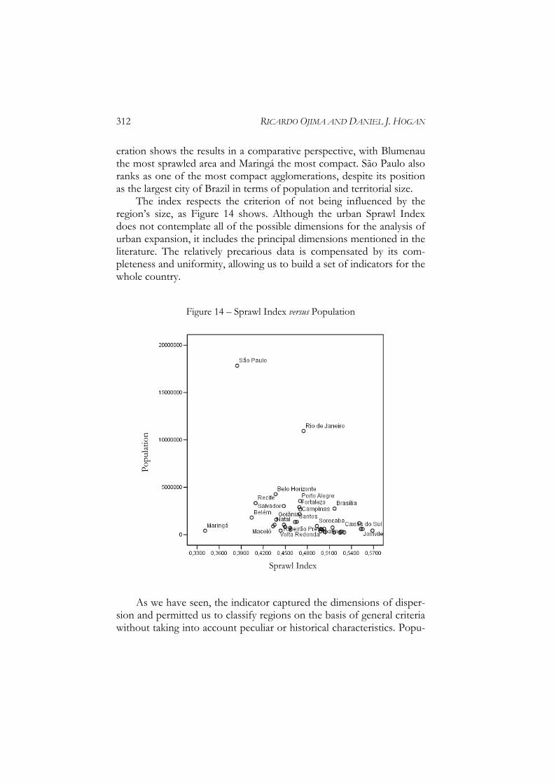
eration shows the results in a comparative perspective, with Blumenau the most sprawled area and Maringá the most compact. São Paulo also ranks as one of the most compact agglomerations, despite its position as the largest city of Brazil in terms of population and territorial size. The index respects the criterion of not being influenced by the region’s size, as Figure 14 shows. Although the urban Sprawl Index does not contemplate all of the possible dimensions for the analysis of urban expansion, it includes the principal dimensions mentioned in the literature. The relatively precarious data is compensated by its com-pleteness and uniformity, allowing us to build a set of indicators for the whole country.

Figure 14 – Sprawl Index versus Population

As we have seen, the indicator captured the dimensions of disper-sion and permitted us to classify regions on the basis of general criteria without taking into account peculiar or historical characteristics. Popu-

Pop

ulat

ion

Sprawl Index


lation size, contradicting some expectations, is not positively correlated with the degree of sprawl. The most dispersed areas are found in the South-Southeast portion of the country, except for Brasília; that is, the most developed region of the country, with a dense network of high-ways. Urban agglomerations located in the North and Northeast are all among the most compact, except for Fortaleza, which is in the inter-mediate group. This can probably be explained by regional characteris-tics of economic integration, expansion of transportation technology or even by overarching globalization processes. Independently of the answer in each case, it is a finding which merits further investigation, following this first effort of comparative analysis. A statistical correlation was found with the proportion of homes with at least one automobile. In other words, the higher the sprawl, the larger the proportion of homes with at least one automobile. That re-sult was expected, since the literature already pointed to that tendency, which, indeed, seems obvious. If an area has greater urban dispersion, the need for transportation should also be greater. Especially in a de-veloping country, household income has an important role in this re-gard, although the same negative correlation is found in all classes of per capita income. From households with lower per capita income up to those with more than 2 minimum wages per person, the correlation is statistically significant. More dispersed urban agglomerations have a larger proportion of automobiles, independently of income. These results raise important challenges for the future of sustain-able urbanization in post-transitional countries, considering that ur-banization is now at a turning point. Urban areas are increasingly complex, with fragmentation, integration and intensification of com-muting. New migration flows are becoming more evident and probably will have a very marked impact on urban structures, especially in terms of access to public services by the poor. Many social problems typical of developing countries become worse with sprawl. If we all expect to live in urban areas by the end of this century, what would be the best urban form for a sustainable world? What are the specific impacts of this kind of urbanization in developing coun-tries? An analysis of the world’s most well-known cities rarely consid-ers the diversity of urban realities, a diversity which becomes more and more relevant in developing countries. Results appear to tell us that urban agglomerations in Brazil have an important commuting element related to sprawling urbanization. These sprawling regions are trans-


forming land use, reducing green and open spaces around cities and increasing automobile dependence, air pollution and costs of public services. New challenges are posed for urbanization in developing countries and if we are unable to understand this process and its con-sequences in the near future, we can expect to see these countries face old problems (poverty) and new problems (sprawl) simultaneously. 5. Policy recommendations: conceptualization, data collection/

management and policy response The questions raised in this discussion suggest the need for action at several levels. In the urban century which awaits us, it will not only be the population of cities but their form which will determine sus-tainability. Morphology matters. It matters for the quality of life of city-dwellers and it matters for the quality and integrity of the natural world. More attention, therefore, must be paid to describing, measur-ing and comparing the spatial distribution of urban populations. This requires, in the first place, that researchers seek greater conceptual and methodological clarity. Many different expressions are in use to denote more dispersed population patterns. While some of these may be im-precise or reflect different research traditions without reflecting sub-stantive differences, several expressions reflect empirically different phenomena. There is little clarity in the literature about what these might be. More intense efforts to sort out the different concepts will be needed to direct data collection which includes urban form. The availability of standardized data in existent data bases, necessary though it may be, will be possible only when there is more agreement on the most useful concepts and measurements. One thing is clear: there is considerable consensus on the envi-ronmental and social benefits of urban morphologies which maximize access to services while minimizing environmental impact. It will be necessary, however, to go beyond such generalizations to arrive at poli-cies which effectively direct city growth. Comparative work is essential. In highly urbanized regions (USA, Europe, Latin America), there is urban infrastructure already in place which will require adaptation in the light of new technologies and new values. In those areas which still expect considerable demographic growth of cities (Asia, Africa), the planning needs are even greater, though potentially more viable and


rewarding: not exactly learning from the mistakes of others, but not making the mistake of adopting 20th century approaches to solving 21st century challenges. Goals and values must be clear. Considering the diversity of ur-ban forms in the contemporary world, it seems evident that quality of life is not irrevocably tied to a single pattern. If greater urban densities have been found compatible with quality of life in some places, and if such densities promote a more sustainable and resilient relationship with the natural world, then it is not unthinkable that they be replicated in other settings. Reordering priorities in favor of sustainable urbaniza-tion involves value changes which cannot be taken for granted. Gov-ernments, international organizations, NGOs and researchers have their mutually reinforcing roles. The techniques of urban planning will have to evolve in parallel with the evolution of the values appropriate to sustainability. Acknowledgements We would like to thank CICRED, PERN and APHRC for supporting participation in the workshop held in Nairobi, Alisson F. Barbieri and Alex de Sherbinin for their suggestions for the final version of this paper. References Angel, S, Sheppard, S C, and Civco, D L (2005) The Dynamics of Global Urban Expan-

sion, Transport and Urban Development Department, The World Bank, Washing-ton DC.

ARCGIS 9.0. Environmental Systems Research Institute, Inc. (ESRI). Baeninger, R A (2004) “Interiorização da migração em São Paulo: novas territoriali-

dades e novos desafios teóricos”, in Anais do XIV Encontro Nacional de Estudos Populacionais, 20-24 de setembro de 2004, Caxambu-MG, ABEP.

Batty, M, Xie, Y, and Sun, Z (1999) The Dynamics of Urban Sprawl, Center for Ad-vanced Spatial Analysis (CASA), Paper 15, University College London, London.

Chin, N (2002) Unearthing the Roots of Urban Sprawl: A Critical Analysis of Form, Function and Methodology, Center for Advanced Spatial Analysis (CASA), Paper 47, Univer-sity College London, London.

Cutsinger, J, Galster, G, Wolman, H, Hanson, R, and Towns, D (2005) “Verifying the Multi-dimensional Nature of Metropolitan Land Use: Advancing the Under-standing and Measurement of Sprawl”, Journal of Urban Affairs, 27(3): 235-259.


Galster, G, Hanson, R, Wolman, H, Coleman, S, and Freihage, J (2001) “Wrestling Sprawl to the Ground: Defining and Measuring an Elusive Concept”, Housing Pol-icy Debate, 12(4): 681-717.

Garcia, R A, and Matos, R (2005) “Densidade populacional urbana e fluxos mi-gratórios: um modelo de estimação da área urbana dos municípios brasileiros”, IV Encontro Nacional sobre Migração, ABEP, Rio de Janeiro.

Giddens, A (1991) The Consequences of Modernity, Polity Press, Basil-Blackwell. Hogan, D J (1993) “População, pobreza e poluição em Cubatão, São Paulo”, in G.

Martine (org.) População, Meio Ambiente e Desenvolvimento, Ed. Unicamp, Campinas, 101-131.

IPEA/IBGE/UNICAMP (2000) Características e Tendências da Rede Urbana no Brasil, Instituto de Economia, UNICAMP, Campinas.

Kampel, S A (2003) Geoinformação para estudos demográficos: representação espacial de dados de população na Amazônia brasileira, PhD dissertation, Universidade de São Paulo.

Kiefer, M J (2003) “Suburbia and its Discontents”, Harvard Design Magazine, 19: 1-5. Lopez, R, and Hynes, H P (2003) “Sprawl in the 1990s: Measurement, Distribution

and Trends”, Urban Affairs Review, 38(3): 325-355. Meadows, D H (1999) “So what can we do – really do – about sprawl”, in Sprawl

Articles, Sierra Club, http://www.sierraclub.org/sprawl/articles/meadows3.asp. Ojima, R (2007) Análise comparativa da dispersão urbana nas aglomerações urbanas brasileiras:

elementos teóricos e metodológicos para o planejamento urbano e ambiental, PhD dissertation, Campinas.

Richardson, H W, and Chang-Hee, C B (eds) (2004), Urban Sprawl in Western Europe and the United States, Ashgate Publishing Limited, England.

Roca, J, Burns, M C, and Carreras, J M (2004) “Monitoring Urban Sprawl Around Barcelona’s Metropolitan Area with the Aid of Satellite Imagery”, XXth ISPRS Congress, 12-23 July, Istanbul, Turkey.

Torrens, P M, and Alberti, M (2000) Measuring Sprawl, Center for Advanced Spatial Analysis (CASA), Paper 27, University College London, London.

Documents

MOBILITY, URBAN SPRAWL AND ENVIRONMENTAL … · ENVIRONMENTAL RISKS IN BRAZILIAN URBAN AGGLOMERATIONS: CHALLENGES FOR URBAN ... tific and Technological ... transportation is also