Embed Size (px)
DESCRIPTION
Mixed Models 1
Citation preview
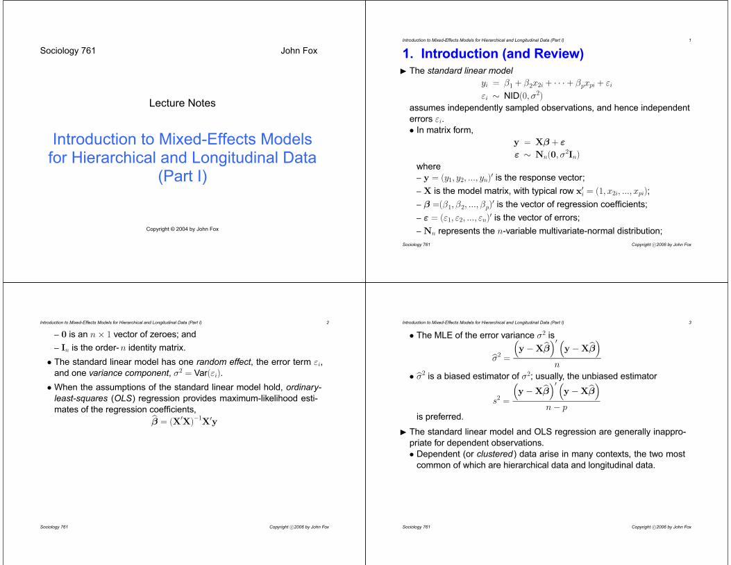
Sociology 761 John Fox
Lecture Notes
Introduction to Mixed-Effects Modelsfor Hierarchical and Longitudinal Data
(Part I)
Copyright © 2004 by John Fox
Introduction to Mixed-Effects Models for Hierarchical and Longitudinal Data (Part I) 1
1. Introduction (and Review)I The standard linear model
= 1 + 2 2 + · · · + +
NID(0 2)
assumes independently sampled observations, and hence independent
errors .
• In matrix form,
y = X +
N (0 2I )
where
– y = ( 1 2 )0 is the response vector;
– X is the model matrix, with typical row x0 = (1 2 );
– =( 1 2 )0 is the vector of regression coefficients;
– = ( 1 2 )0 is the vector of errors;
– N represents the -variable multivariate-normal distribution;
Sociology 761 Copyright c°2006 by John Fox
Introduction to Mixed-Effects Models for Hierarchical and Longitudinal Data (Part I) 2
– 0 is an × 1 vector of zeroes; and
– I is the order- identity matrix.
• The standard linear model has one random effect, the error term ,
and one variance component, 2 = Var( ).
• When the assumptions of the standard linear model hold, ordinary-
least-squares (OLS) regression provides maximum-likelihood esti-
mates of the regression coefficients,b = (X0X) 1
X0y
Sociology 761 Copyright c°2006 by John Fox
Introduction to Mixed-Effects Models for Hierarchical and Longitudinal Data (Part I) 3
• The MLE of the error variance 2 is
b2 =³y Xb´0 ³y Xb´
• b2 is a biased estimator of 2; usually, the unbiased estimator
2 =
³y Xb´0 ³y Xb´
is preferred.
I The standard linear model and OLS regression are generally inappro-
priate for dependent observations.
• Dependent (or clustered) data arise in many contexts, the two most
common of which are hierarchical data and longitudinal data.
Sociology 761 Copyright c°2006 by John Fox

Introduction to Mixed-Effects Models for Hierarchical and Longitudinal Data (Part I) 4
I Hierarchical data are collected when sampling takes place at two or
more levels, one nested within the other. Some examples:
• Students within schools (two levels).
• Students within classrooms within schools (three levels).
• Individuals within nations (two levels).
• Individuals within communities within nations (three levels).
• Patients within physicians (two levels).
• Patients within physicians within hospitals (three levels).
I There can also be non-nested multi-level data — for example, high-
school students who each have multiple teachers.
Sociology 761 Copyright c°2006 by John Fox
Introduction to Mixed-Effects Models for Hierarchical and Longitudinal Data (Part I) 5
I Longitudinal data are collected when individuals (or other units of
observation) are followed over time. Some examples:
• Annual data on vocabulary growth among children.
• Biannual data on weight-preoccupation and exercise among adoles-
cent girls.
• Data collected at irregular intervals on recovery of IQ among coma
patients.
• Annual data on employment and income for a sample of adult
Canadians.
I In all of these cases, it is not generally reasonable to assume that ob-
servations within the same higher-level unit, or longitudinal observations
within the same individual, are independent of one-another.
Sociology 761 Copyright c°2006 by John Fox
Introduction to Mixed-Effects Models for Hierarchical and Longitudinal Data (Part I) 6
I Mixed-effect models make it possible to take account of dependencies
in hierarchical, longitudinal, and other dependent data.
• Unlike the standard linear model, mixed-effect models include more
than one source of random variation — i.e., more than one random
effect.
• Mixed-effects models have been developed in a variety of disciplines,
with varying names and terminology: random-effects models (sta-
tistics, econometrics), variance and covariance-component models
(statistics), hierarchical linear models (education), multi-level models
(sociology), contextual-effects models (sociology), random-coefficient
models (econometrics), repeated-measures models (statistics, psy-
chology).
• Mixed-effects models have a long history, dating to Fisher and Yates’s
work on “split-plot” agricultural experiments.
Sociology 761 Copyright c°2006 by John Fox
Introduction to Mixed-Effects Models for Hierarchical and Longitudinal Data (Part I) 7
• What distinguishes modern mixed models from their predecessors
is generality: for example, the ability to accommodate irregular and
missing observations.
Sociology 761 Copyright c°2006 by John Fox

Introduction to Mixed-Effects Models for Hierarchical and Longitudinal Data (Part I) 8
I Principal sources for these lectures on mixed models:
• Stephen Raudenbush and Anthony Bryk, Hierarchical Linear Models,
Second Edition, Sage, 2002.
• Jose Pinheiro and Douglas Bates, Mixed-Effects Models in S and
S-PLUS, Springer, 2000.
I Topics:
• The linear mixed-effects model.
• Modeling hierarchical data.
• Modeling longitudinal data.
• Generalized linear mixed models (time permitting).
Sociology 761 Copyright c°2006 by John Fox
Introduction to Mixed-Effects Models for Hierarchical and Longitudinal Data (Part I) 9
2. The Linear Mixed-Effects ModelI This section introduces a very general linear mixed model, which we will
adapt to particular circumstances.
I The Laird-Ware form of the linear mixed model:
= 1 + 2 2 + · · · + + 1 1 + · · · + +
(0 2) Cov( 0 ) = 0
0 0 are independent for 6= 0
(0 2 ) Cov( 0) = 20
0 0 are independent for 6= 0
where
• is the value of the response variable for the th of observations
in the th of groups or clusters.
• 1 2 are the fixed-effect coefficients, which are identical for all
groups.
Sociology 761 Copyright c°2006 by John Fox
Introduction to Mixed-Effects Models for Hierarchical and Longitudinal Data (Part I) 10
• 2 are the fixed-effect regressors for observation in group
; there is also implicitly a constant regressor, 1 = 1.
• 1 are the random-effect coefficients for group , assumed
to be multivariately normally distributed, independent of the random
effects of other groups. The random effects, therefore, vary by group.
– The are thought of as random variables, not as parameters, and
are similar in this respect to the errors .
• 1 are the random-effect regressors.
– The ’s are almost always a subset of the ’s (and may include all of
the ’s).
– When there is a random intercept term, 1 = 1.
• 2 are the variances and 0 the covariances among the random
effects, assumed to be constant across groups.
– In some applications, the ’s are parametrized in terms of a smaller
number of fundamental parameters.
Sociology 761 Copyright c°2006 by John Fox
Introduction to Mixed-Effects Models for Hierarchical and Longitudinal Data (Part I) 11
• is the error for observation in group
– The errors for group are assumed to be multivariately normally
distributed, and independent of errors in other groups.
• 20 are the covariances between errors in group .
– Generally, the 0 are parametrized in terms of a few basic
parameters, and their specific form depends upon context.
– When observations are sampled independently within groups and
are assumed to have constant error variance (as is typical in
hierarchical models), = 1, 0 = 0 (for 6= 0), and thus the only
free parameter to estimate is the common error variance, 2.
– If the observations in a “group” represent longitudinal data on a
single individual, then the structure of the ’s may be specified to
capture serial (i.e., over-time) dependencies among the errors.
Sociology 761 Copyright c°2006 by John Fox

Introduction to Mixed-Effects Models for Hierarchical and Longitudinal Data (Part I) 12
I The Laird-Ware model in matrix form:
y = X + Z b +
b N (0 )
b b 0 are independent for 6= 0
N (0 2 )
0 are independent for 6= 0
where
• y is the × 1 response vector for observations in the th group.
• X is the × model matrix for the fixed effects for observations in
group .
• is the × 1 vector of fixed-effect coefficients.
• Z is the × model matrix for the random effects for observations in
group
• b is the × 1 vector of random-effect coefficients for group .
• is the × 1 vector of errors for observations in group .
Sociology 761 Copyright c°2006 by John Fox
Introduction to Mixed-Effects Models for Hierarchical and Longitudinal Data (Part I) 13
• is the × covariance matrix for the random effects.
• 2 is the × covariance matrix for the errors in group , and is2I if the within-group errors are homoscedastic and independent.
I Notice that there are two things that distinguish the linear mixed model
from the standard linear model:
(1) There are structured random effects b in addition to the errors .
(2) The model can accommodate heteroscedasticity and dependencies
among the errors.
Sociology 761 Copyright c°2006 by John Fox
Introduction to Mixed-Effects Models for Hierarchical and Longitudinal Data (Part I) 14
3. Modeling Hierarchical DataI Applications of mixed models to hierarchical data have become common
in the social sciences, and nowhere more so than in research on
education.
I I’ll restrict myself to two-level models, but three or more levels can also
be handled through an extension of the Laird-Ware model.
I The following example is borrowed from Raudenbush and Bryk, and has
been used by others as well (though we will learn some things about the
data that apparently haven’t been noticed before).
• The data are from the 1982 “High School and Beyond” survey, and
pertain to 7185 U.S. high-school students from 160 schools — about
45 students on average per school.
– 70 of the high schools are Catholic schools and 90 are public
schools.
Sociology 761 Copyright c°2006 by John Fox
Introduction to Mixed-Effects Models for Hierarchical and Longitudinal Data (Part I) 15
• The object of the data analysis is to determine how students’ math
achievement scores are related to their family socioeconomic status.
– We will entertain the possibility that the level of math achievement
and the relationship between achievement and SES vary among
schools.
– If there is evidence of variation among schools, we will examine
whether this variation is related to school characteristics — in
particular, whether the school is a public school or a Catholic school
and the average SES of students in the school.
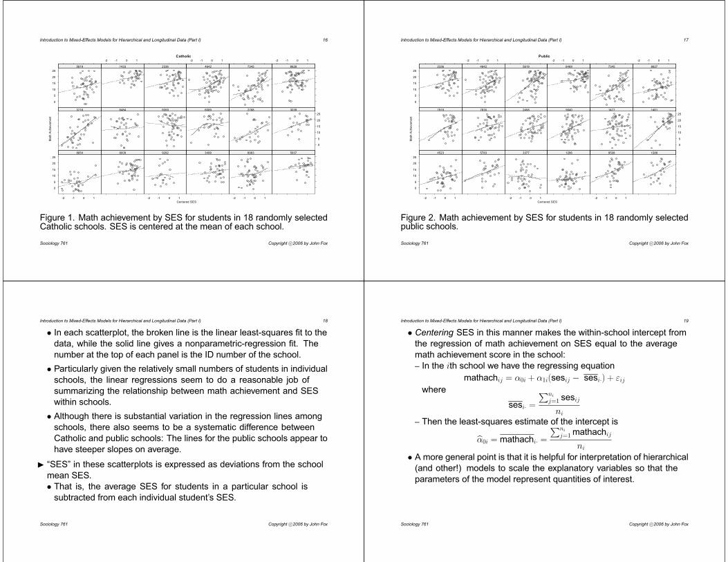
I A good place to start is to examine the relationship between math
achievement and SES separately for each school.
• 160 schools are too many to look at individually, so I sampled 18
Catholic school and 18 public schools at random.
• The scatterplots for the sampled schools are in Figures 1 and 2.
Sociology 761 Copyright c°2006 by John Fox
Introduction to Mixed-Effects Models for Hierarchical and Longitudinal Data (Part I) 16
Catholic
Centered SES
Math
Achie
vem
ent
0
5
10
15
20
25
-2 -1 0 1
8854 8009
-2 -1 0 1
9292 3499
-2 -1 0 1
8983 5937
3716 6484 9359 6089 2768
0
5
10
15
20
25
3039
0
5
10
15
20
25
5819 1433
-2 -1 0 1
2336 4642
-2 -1 0 1
7345 8628
-2 -1 0 1
Figure 1. Math achievement by SES for students in 18 randomly selectedCatholic schools. SES is centered at the mean of each school.
Sociology 761 Copyright c°2006 by John Fox
Introduction to Mixed-Effects Models for Hierarchical and Longitudinal Data (Part I) 17
Public
Centered SES
Math
Achie
vem
ent
0
5
10
15
20
25
-2 -1 0 1
4523 5783
-2 -1 0 1
3377 1296
-2 -1 0 1
9508 1288
7919 7635 2458 5640 1477
0
5
10
15
20
25
1461
0
5
10
15
20
25
2336 4642
-2 -1 0 1
5619 6469
-2 -1 0 1
7345 8627
-2 -1 0 1
Figure 2. Math achievement by SES for students in 18 randomly selectedpublic schools.
Sociology 761 Copyright c°2006 by John Fox
Introduction to Mixed-Effects Models for Hierarchical and Longitudinal Data (Part I) 18
• In each scatterplot, the broken line is the linear least-squares fit to the
data, while the solid line gives a nonparametric-regression fit. The
number at the top of each panel is the ID number of the school.
• Particularly given the relatively small numbers of students in individual
schools, the linear regressions seem to do a reasonable job of
summarizing the relationship between math achievement and SES
within schools.
• Although there is substantial variation in the regression lines among
schools, there also seems to be a systematic difference between
Catholic and public schools: The lines for the public schools appear to
have steeper slopes on average.
I “SES” in these scatterplots is expressed as deviations from the school
mean SES.
• That is, the average SES for students in a particular school is
subtracted from each individual student’s SES.
Sociology 761 Copyright c°2006 by John Fox
Introduction to Mixed-Effects Models for Hierarchical and Longitudinal Data (Part I) 19
• Centering SES in this manner makes the within-school intercept from
the regression of math achievement on SES equal to the average
math achievement score in the school:
– In the th school we have the regressing equation
mathach = 0 + 1 (ses ses ·) +
where
ses · =
P=1
ses
– Then the least-squares estimate of the intercept is
b0 = mathach · =
P=1
mathach
• A more general point is that it is helpful for interpretation of hierarchical
(and other!) models to scale the explanatory variables so that the
parameters of the model represent quantities of interest.
Sociology 761 Copyright c°2006 by John Fox
Introduction to Mixed-Effects Models for Hierarchical and Longitudinal Data (Part I) 20
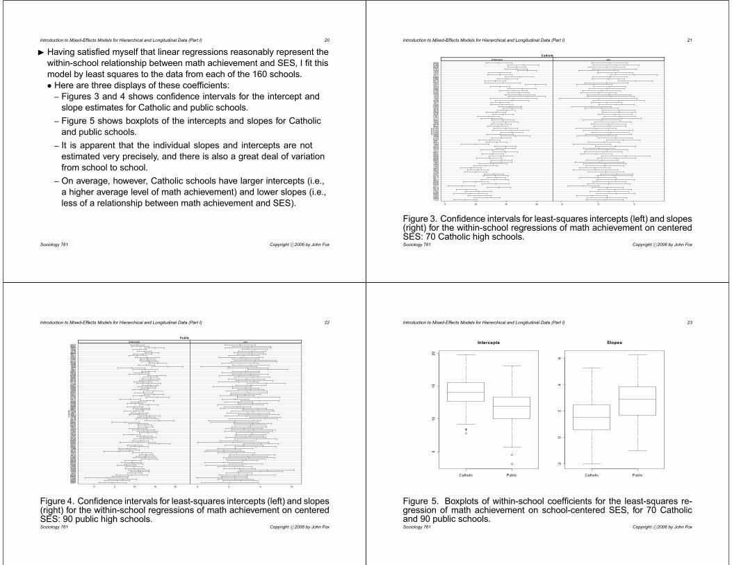
I Having satisfied myself that linear regressions reasonably represent the
within-school relationship between math achievement and SES, I fit this
model by least squares to the data from each of the 160 schools.
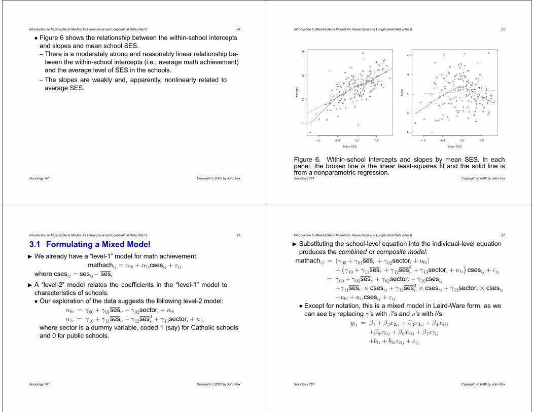
• Here are three displays of these coefficients:
– Figures 3 and 4 shows confidence intervals for the intercept and
slope estimates for Catholic and public schools.
– Figure 5 shows boxplots of the intercepts and slopes for Catholic
and public schools.
– It is apparent that the individual slopes and intercepts are not
estimated very precisely, and there is also a great deal of variation
from school to school.
– On average, however, Catholic schools have larger intercepts (i.e.,
a higher average level of math achievement) and lower slopes (i.e.,
less of a relationship between math achievement and SES).
Sociology 761 Copyright c°2006 by John Fox
Introduction to Mixed-Effects Models for Hierarchical and Longitudinal Data (Part I) 21
Catholic
school
||
||
||
||
||
||
||
||
||
|||
||
||
||
||
||
||
||
||
||
||
||
||
||
|||
||
||
||
||
|||
||
||
||
||
|
||
||
||
||
||
||
||
||
||
|||
||
||
|||
||
||
||
||
||
||
||
||
||
||
||
||
||
||
||
||
||
|||
|||
||
||
||
||
||
||
||
||
||
||
|||
||
||
|||
||
||
||
||
||
||
||
||
||
||
||
||
||
||
||
||
||
||
||
||
||
5 10 15 20
7172486823058800519245236816227780094530902145116578934737053533425373423499736456502658950842928857131726294223146249315667572034983688816591048150404260741906399241735761763524583610383893592208147730391308143314362526275529903020342754045619636664697011733276888193862891989586
(Intercept)
||
||
||
||
||
||
||
||
||
||
||
||
||
||
||
||
||
||
||
||
||
||
||
||
||
||
||
||
||
||
|||
||
||
||
|
||
||
||
||
||
||
||
||
|||
||
||
||
||
||
||
||
||
||
||
||
||
|||
||
||
||
||
||
||
||
||
||
||
||
||
||
||
||
||
||
||
||
||
||
||
||
||
||
||
||
||
||
||
|||
||
||
|||
||
||
||
||
||
||
||
||
||
||
||
||
-5 0 5
ses
Figure 3. Confidence intervals for least-squares intercepts (left) and slopes(right) for the within-school regressions of math achievement on centeredSES: 70 Catholic high schools.Sociology 761 Copyright c°2006 by John Fox
Introduction to Mixed-Effects Models for Hierarchical and Longitudinal Data (Part I) 22
Public
school
||
||
||
||
|||
||
||
||
||
||
||
||
||
||
||
||
||
||
||
||
||
||
||
||
||
||
||
||
||
||
||
||
||
||
||
||
||
||
||
||
||
||
||
||
|
||
||
||
||
||
||
||
||
|||
||
||
||
||
||
||
||
||
||
||
||
||
||
||
||
||
||
||
||
||
||
||
||
||
||
||
||
||
||
||
|||
||
||
||
||
||
|||
||
||
||
||
||
||
||
||
||
||
||
||
||
||
||
||
||
||
||
||
||
||
||
||
||
||
||
||
||
||
||
||
|||
||
||
||
||
||
||
||
||
||
0 5 10 15 20
836788544458576269905815734113584383308887757890614464436808281893405783301371012639337712964350939726559292898381884410870714998477128862911224396764159550646459377919371619092651246713746600388129955838915889467232291761702030835785314420399943256484689777348175887492255640608927685819639714611637194219462336262627713152333233513657464272767345769782028627
(Intercept)
||
||
||
||
||
||
||
||
||
||
||
||
||
||
||
|||
||
||
||
||
||
||
||
||
||
||
||
||
||
||
||
||
||
||
||
||
||
||
||
||
||
||
||
||
|
||
||
||
||
||
||
||
||
||
||
||
||
||
||
||
||
||
||
||
|||
||
||
||
||
||
||
||
||
||
||
||
||
||
||
||
||
||
||
||
||
||
||
||
||
|
||
|||
||
||
||
||
||
||
||
||
||
||
||
||
||
||
||
|||
||
||
||
||
||
||
||
||
||
||
||
||
||
||
||
||
|||
||
||
||
||
||
||
||
||
|
-5 0 5 10
ses
Figure 4. Confidence intervals for least-squares intercepts (left) and slopes(right) for the within-school regressions of math achievement on centeredSES: 90 public high schools.Sociology 761 Copyright c°2006 by John Fox
Introduction to Mixed-Effects Models for Hierarchical and Longitudinal Data (Part I) 23
Catholic Public
51
01
52
0
Intercepts
Catholic Public
-20
24
6
Slopes
Figure 5. Boxplots of within-school coefficients for the least-squares re-gression of math achievement on school-centered SES, for 70 Catholicand 90 public schools.Sociology 761 Copyright c°2006 by John Fox
Introduction to Mixed-Effects Models for Hierarchical and Longitudinal Data (Part I) 24
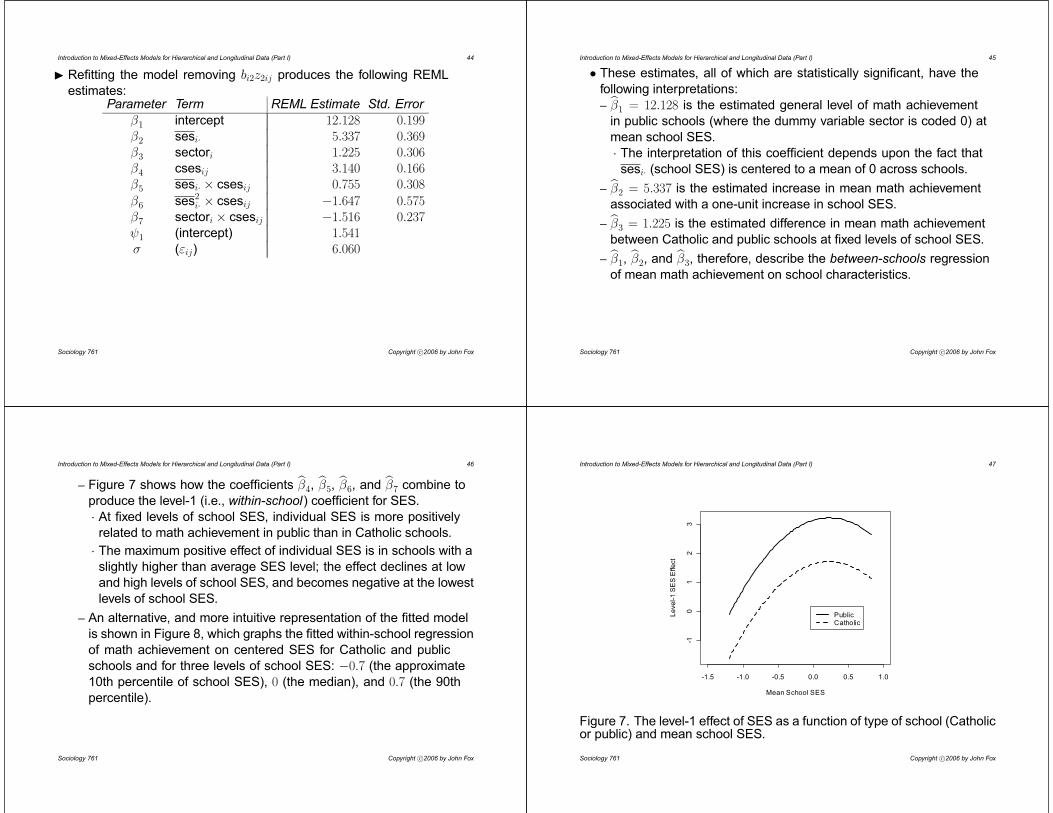
• Figure 6 shows the relationship between the within-school intercepts
and slopes and mean school SES.
– There is a moderately strong and reasonably linear relationship be-
tween the within-school intercepts (i.e., average math achievement)
and the average level of SES in the schools.
– The slopes are weakly and, apparently, nonlinearly related to
average SES.
Sociology 761 Copyright c°2006 by John Fox
Introduction to Mixed-Effects Models for Hierarchical and Longitudinal Data (Part I) 25
-1.0 -0.5 0.0 0.5
51
01
52
0
Mean SES
Inte
rce
pt
-1.0 -0.5 0.0 0.5
-20
24
6
Mean SES
Slo
pe
Figure 6. Within-school intercepts and slopes by mean SES. In eachpanel, the broken line is the linear least-squares fit and the solid line isfrom a nonparametric regression.Sociology 761 Copyright c°2006 by John Fox
Introduction to Mixed-Effects Models for Hierarchical and Longitudinal Data (Part I) 26
3.1 Formulating a Mixed Model
I We already have a “level-1” model for math achievement:
mathach = 0 + 1 cses +
where cses = ses ses ·
I A “level-2” model relates the coefficients in the “level-1” model to
characteristics of schools.
• Our exploration of the data suggests the following level-2 model:
0 = 00 + 01ses · + 02sector + 0
1 = 10 + 11ses · + 12ses2· + 13sector + 1
where sector is a dummy variable, coded 1 (say) for Catholic schools
and 0 for public schools.
Sociology 761 Copyright c°2006 by John Fox
Introduction to Mixed-Effects Models for Hierarchical and Longitudinal Data (Part I) 27
I Substituting the school-level equation into the individual-level equation
produces the combined or composite model:
mathach = ( 00 + 01ses · + 02sector + 0 )
+¡10 + 11ses · + 12ses2· + 13sector + 1
¢cses +
= 00 + 01ses · + 02sector + 10cses
+ 11ses · × cses + 12ses2· × cses + 13sector × cses
+ 0 + 1 cses +
• Except for notation, this is a mixed model in Laird-Ware form, as we
can see by replacing ’s with ’s and ’s with ’s:
= 1 + 2 2 + 3 3 + 4 4
+ 5 5 + 6 6 + 7 7
+ 1 + 2 2 +
Sociology 761 Copyright c°2006 by John Fox

Introduction to Mixed-Effects Models for Hierarchical and Longitudinal Data (Part I) 28
• Note that all explanatory variables in the Laird-Ware form of the model
carry subscripts for schools and individuals within schools, even
when the explanatory variable in question is constant within schools.
– Thus, for example, 2 = ses · (and so all individuals in the same
school share a common value of school-mean SES).
– There is both a data-management issue here and a conceptual
point:
– With respect to data management, software that fits the Laird-Ware
form of the model (such as the lme or lmer functions in R) requires
that level-2 explanatory variables (here sector and school-mean
SES, which are characteristics of schools) appear in the level-1 (i.e.,
student) data set — much as the person × time-period data set
that we employed in survival analysis with time-varying covariates
required that time-constant covariates appear on the data record for
each time period.
Sociology 761 Copyright c°2006 by John Fox
Introduction to Mixed-Effects Models for Hierarchical and Longitudinal Data (Part I) 29
– The conceptual point is that the model can incorporate contextual
effects — characteristics of the level-2 units can influence the level-1
response variable.
– Such contextual effects are of two kinds:
· Compositional effects, such as the effect of school-mean SES,
which are composed from characteristics of individuals within a
level-2 unit.
· Effects of characteristics of the level-2 units, such as school sector,
that do not pertain to the level-1 units.
I Rather than proceeding with this relatively complicated model, let us
first investigate some simpler mixed-effects models derived from it.
Sociology 761 Copyright c°2006 by John Fox
Introduction to Mixed-Effects Models for Hierarchical and Longitudinal Data (Part I) 30
3.1.1 Random-Effects One-Way Analysis of Variance
I Consider the following level-1 and level-2 models:
mathach = 0 +
0 = 00 + 0
I The combined model is
mathach = 00 + 0 +
• In Laird-Ware form:
= 1 + 1 +
I This is a random-effects one-way ANOVA model with one fixed effect,
1, representing the general population mean of math achievement, and
two random effects:
• 1 , representing the deviation of math achievement in school from
the general mean; that is, = 1 + 1 is mean math achievement in
school .
Sociology 761 Copyright c°2006 by John Fox
Introduction to Mixed-Effects Models for Hierarchical and Longitudinal Data (Part I) 31
• , representing the deviation of individual ’s math achievement in
school from the school mean.
• Two observations and 0 in school are not independent because
they share the random effect, 1 .
I There are also two variance components for this model:
• 2
1 = Var( 1 ) is the variance among school means.
• 2 = Var( ) is the variance among individuals in the same school.
I Because the 1 and are assumed to be independent, variation in
math scores among individuals can be decomposed into these two
variance components:
Var( ) =£( 1 + )2
¤= 2
1 +2
[since ( 1 ) = ( ) = 0, and hence ( ) = 1].
Sociology 761 Copyright c°2006 by John Fox

Introduction to Mixed-Effects Models for Hierarchical and Longitudinal Data (Part I) 32
• The intra-class correlation coefficient is the proportion of variation in
individuals’ scores due to differences among schools:
=2
1
Var( )=
2
1
2
1 +2
• may also be interpreted as the correlation between the math scores
of two individuals from the same school. That is,
Cov( 0) = [( 1 + )( 1 + 0)] = ( 21 ) =2
1
Var( ) = Var( 0) = 2
1 +2
Cor( 0) =Cov( 0)p
Var( )× Var( 0)=
2
1
2
1 +2=
Sociology 761 Copyright c°2006 by John Fox
Introduction to Mixed-Effects Models for Hierarchical and Longitudinal Data (Part I) 33
I The lme function in the nlme package in R provides two methods to
estimate mixed-effects models (as does the lmer function in the lme2
package):
• Full maximum-likelihood (ML) estimation of the model maximizes
the likelihood with respect to all of the parameters of the model
simultaneously (i.e., both the fixed-effects parameters and the
variance components).
• Restricted (or residual) maximum-likelihood (REML) estimation
integrates the fixed effects out of the likelihood and estimates
the variance components; given the estimates of the variance
components, estimates of the fixed effects are recovered.
• A disadvantage of ML estimates of variance components is that they
are biased downwards in finite samples (much as the ML estimate of
the error variance in the standard linear model is biased downwards).
• The REML estimates, in contrast, correct for loss of degrees of
freedom due to estimating the fixed effects.
Sociology 761 Copyright c°2006 by John Fox
Introduction to Mixed-Effects Models for Hierarchical and Longitudinal Data (Part I) 34
• The difference between the ML and REML estimates can be important
when the number of “clusters” (i.e., level-2 units) in the data is small.
I ML and REML estimates for the current example, where there are 160
schools (level-2 units), are nearly identical:
Parameter ML Estimate REML Estimate
1 12 637 12 637
1 2 925 2 9356 257 6 257
• Note that the standard deviations (rather than the variances) of the
random effects are shown.
• The estimated intra-class correlation coefficient is
b = 2 9352
2 9352 + 6 2572= 0 180
and so 18 percent of the variation in students’ math-achievement
scores is “attributable” to differences among schools.
Sociology 761 Copyright c°2006 by John Fox
Introduction to Mixed-Effects Models for Hierarchical and Longitudinal Data (Part I) 35
3.1.2 Random-Coefficients Regression Model
I Let us introduce school-centered SES into the level-1 model as an
explanatory variable,
mathach = 0 + 1 cses +
and allow for random intercepts and slopes in the level-2 model:
0 = 00 + 0
1 = 10 + 1
I The combined model is now
mathach = ( 00 + 0 ) + ( 10 + 1 ) cses +
= 00 + 10cses + 0 + 1 cses +
• In Laird-Ware form:
= 1 + 2 2 + 1 + 2 2 +
I This model is a random-coefficients regression model.
Sociology 761 Copyright c°2006 by John Fox

Introduction to Mixed-Effects Models for Hierarchical and Longitudinal Data (Part I) 36
I The fixed-effects coefficients 1 and 2 represent, respectively, the
average within-schools population intercept and slope.
• Because SES is centered within schools, the intercept 1 represents
the general level of math achievement in the population (in the sense
of the average within-school mean).
I The model has four variance-covariance components:
• 2
1 = Var( 1 ) is the variance among school intercepts (i.e., school
means, because SES is school-centered).
• 2
2 = Var( 2 ) is the variance among within-school slopes.
• 12 = Cov( 1 2 ) is the covariance between within-school intercepts
and slopes.
• 2 = Var( ) is the error variance around the within-school regres-
sions.
Sociology 761 Copyright c°2006 by John Fox
Introduction to Mixed-Effects Models for Hierarchical and Longitudinal Data (Part I) 37
I The composite error for individual in school is
= 1 + 2 2 +
• The variance of the composite error is
Var( ) = ( 2 ) =£( 1 + 2 2 + )2
¤= 2
1 +2
2
2
2 + 2 2 12 +2
• And the covariance of the composite errors for two individuals and 0
in the same school is
Cov( 0) = ( × 0) = [( 1 + 2 2 + )( 1 + 2 2 0 + 0)]
= 2
1 + 2 2 02
2 + ( 2 + 2 0) 12
• Consequently the composite errors are heteroscedastic, and errors for
individuals in the same school are correlated.
• But the composite errors for two individuals in different schools are
independent.
Sociology 761 Copyright c°2006 by John Fox
Introduction to Mixed-Effects Models for Hierarchical and Longitudinal Data (Part I) 38
I ML and REML estimates for the model are as follows:Parameter ML Estimate Std. Error REML Estimate Std. Error
1 12 636 0 244 12 636 0 245
2 2 193 0 128 2 193 0 128
1 2 936 2 946
2 0 823 0 833
12 0 041 0 0426 058 6 058
• Again, the ML and REML estimates are very close.
• Note that I’ve given standard errors only for the fixed effects.
– Standard errors for variance and covariance components can be
obtained in the usual manner from the inverse of the information
matrix, but tests and confidence intervals based on these standard
errors tend not to be accurate.
Sociology 761 Copyright c°2006 by John Fox
Introduction to Mixed-Effects Models for Hierarchical and Longitudinal Data (Part I) 39
– We can, however, test variance and covariance components by a
likelihood-ratio test, contrasting the (restricted) log-likelihood for the
fitted model with that for a model removing the random effects in
question.
– For example, for the current model (say model 1), removing 2 2
from the model (producing, say, model 0) implies that the SES slope
is identical across schools.
· Removing 2 2 from the model gets rid of two variance-covariance
parameters, 2 and 12.
· A likelihood-ratio test for these parameters suggests that they
should not be omitted from the model:
log 1 = 23 357 12
log 0 = 23 362 002 = 2(log 1 log 0) = 9 76, = 2, = 008
Sociology 761 Copyright c°2006 by John Fox

Introduction to Mixed-Effects Models for Hierarchical and Longitudinal Data (Part I) 40
I Cautionary Remarks:
• Because REML estimates are calculated integrating out the fixed
effects, one cannot legitimately perform likelihood-ratio tests across
models with different fixed effects when the models are estimated by
REML.
– Likelihood-ratio for variance-covariance components across nested
models with identical fixed effects are perfectly fine, however.
• A common source of estimation difficulties in mixed models is the
specification of overly complex random effects.
– Interest usually centers in the fixed effects, and it often pays to try to
simplify the random-effect part of the model.
Sociology 761 Copyright c°2006 by John Fox
Introduction to Mixed-Effects Models for Hierarchical and Longitudinal Data (Part I) 41
3.1.3 Coefficients-as-Outcomes Model
I The regression-coefficients-as-outcomes model introduces explanatory
variables at level 2 to account for variation among the level-1 regression
coefficients. This returns us to the model that we originally formulated
for the math-achievement data:
• at level 1,
mathach = 0 + 1 cses +
• at level 2,
0 = 00 + 01ses · + 02sector + 0
1 = 10 + 11ses · + 12ses2· + 13sector + 1
• The combined model:
mathach = 00 + 01ses · + 02sector + 10cses
+ 11ses · × cses + 12ses2· × cses + 13sector × cses
+ 0 + 1 cses +
Sociology 761 Copyright c°2006 by John Fox
Introduction to Mixed-Effects Models for Hierarchical and Longitudinal Data (Part I) 42
• The combined model in Laird-Ware form:
= 1 + 2 2 + 3 3 + 4 4
+ 5 5 + 6 6 + 7 7
+ 1 + 2 2 +
• This model has more fixed effects than the preceding random-
coefficients regression model, but the same random effects and
variance components: 2
1 = Var( 1 ),2
2 = Var( 2 ), 12 = Cov( 1 2 ),and 2 = Var( ).
I After fitting this model to the data by REML, I tested to check whether
random intercepts and slopes are still required:
Model Omitting log1 — 23 247 702 2
1 12 23 357 863 2
2 12 23 247 93
Sociology 761 Copyright c°2006 by John Fox
Introduction to Mixed-Effects Models for Hierarchical and Longitudinal Data (Part I) 43
• Thus, the test for random intercepts is highly statistically significant,2 = 219 86, = 2, ' 0.
• But the test for random slopes is not, 2 = 0 46, = 2, = 80:Apparently, the level-2 explanatory variables do a sufficiently good job
of accounting for differences in slopes that the variance component for
slopes is no longer needed.
Sociology 761 Copyright c°2006 by John Fox
Introduction to Mixed-Effects Models for Hierarchical and Longitudinal Data (Part I) 44
I Refitting the model removing 2 2 produces the following REML
estimates:Parameter Term REML Estimate Std. Error
1 intercept 12 128 0 199
2 ses · 5 337 0 369
3 sector 1 225 0 306
4 cses 3 140 0 166
5 ses · × cses 0 755 0 308
6 ses2· × cses 1 647 0 575
7 sector × cses 1 516 0 237
1 (intercept) 1 541( ) 6 060
Sociology 761 Copyright c°2006 by John Fox
Introduction to Mixed-Effects Models for Hierarchical and Longitudinal Data (Part I) 45
• These estimates, all of which are statistically significant, have the
following interpretations:
–
b1 = 12 128 is the estimated general level of math achievement
in public schools (where the dummy variable sector is coded 0) at
mean school SES.
· The interpretation of this coefficient depends upon the fact that
ses · (school SES) is centered to a mean of 0 across schools.
–
b2 = 5 337 is the estimated increase in mean math achievement
associated with a one-unit increase in school SES.
–
b3 = 1 225 is the estimated difference in mean math achievement
between Catholic and public schools at fixed levels of school SES.
–
b1,b2, and b3, therefore, describe the between-schools regression
of mean math achievement on school characteristics.
Sociology 761 Copyright c°2006 by John Fox
Introduction to Mixed-Effects Models for Hierarchical and Longitudinal Data (Part I) 46
– Figure 7 shows how the coefficients b4, b5, b6, and b7 combine to
produce the level-1 (i.e., within-school) coefficient for SES.
· At fixed levels of school SES, individual SES is more positively
related to math achievement in public than in Catholic schools.
· The maximum positive effect of individual SES is in schools with a
slightly higher than average SES level; the effect declines at low
and high levels of school SES, and becomes negative at the lowest
levels of school SES.
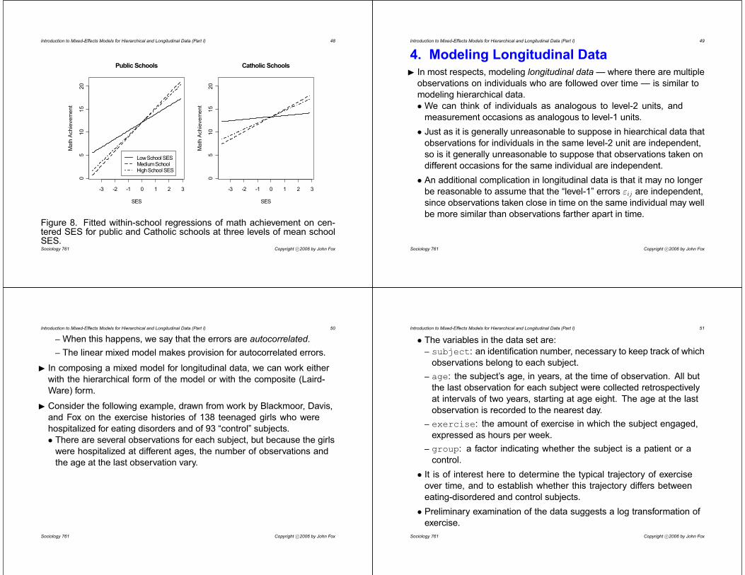
– An alternative, and more intuitive representation of the fitted model
is shown in Figure 8, which graphs the fitted within-school regression
of math achievement on centered SES for Catholic and public
schools and for three levels of school SES: 0 7 (the approximate
10th percentile of school SES), 0 (the median), and 0 7 (the 90th
percentile).
Sociology 761 Copyright c°2006 by John Fox
Introduction to Mixed-Effects Models for Hierarchical and Longitudinal Data (Part I) 47
-1.5 -1.0 -0.5 0.0 0.5 1.0
-10
12
3Mean School SES
Le
ve
l-1
SE
S E
ffe
ct
PublicCatholic
Figure 7. The level-1 effect of SES as a function of type of school (Catholicor public) and mean school SES.
Sociology 761 Copyright c°2006 by John Fox
Introduction to Mixed-Effects Models for Hierarchical and Longitudinal Data (Part I) 48
-3 -2 -1 0 1 2 3
05
10
15
20
Public Schools
SES
Ma
th A
ch
ieve
me
nt
Low School SESMedium SchoolHigh School SES
-3 -2 -1 0 1 2 3
05
10
15
20
Catholic Schools
SESM
ath
Ach
ieve
me
nt
Figure 8. Fitted within-school regressions of math achievement on cen-tered SES for public and Catholic schools at three levels of mean schoolSES.Sociology 761 Copyright c°2006 by John Fox
Introduction to Mixed-Effects Models for Hierarchical and Longitudinal Data (Part I) 49
4. Modeling Longitudinal DataI In most respects, modeling longitudinal data — where there are multiple
observations on individuals who are followed over time — is similar to
modeling hierarchical data.
• We can think of individuals as analogous to level-2 units, and
measurement occasions as analogous to level-1 units.
• Just as it is generally unreasonable to suppose in hiearchical data that
observations for individuals in the same level-2 unit are independent,
so is it generally unreasonable to suppose that observations taken on
different occasions for the same individual are independent.
• An additional complication in longitudinal data is that it may no longer
be reasonable to assume that the “level-1” errors are independent,
since observations taken close in time on the same individual may well
be more similar than observations farther apart in time.
Sociology 761 Copyright c°2006 by John Fox
Introduction to Mixed-Effects Models for Hierarchical and Longitudinal Data (Part I) 50
– When this happens, we say that the errors are autocorrelated.
– The linear mixed model makes provision for autocorrelated errors.
I In composing a mixed model for longitudinal data, we can work either
with the hierarchical form of the model or with the composite (Laird-
Ware) form.
I Consider the following example, drawn from work by Blackmoor, Davis,
and Fox on the exercise histories of 138 teenaged girls who were
hospitalized for eating disorders and of 93 “control” subjects.
• There are several observations for each subject, but because the girls
were hospitalized at different ages, the number of observations and
the age at the last observation vary.
Sociology 761 Copyright c°2006 by John Fox
Introduction to Mixed-Effects Models for Hierarchical and Longitudinal Data (Part I) 51
• The variables in the data set are:
– subject: an identification number, necessary to keep track of which
observations belong to each subject.
– age: the subject’s age, in years, at the time of observation. All but
the last observation for each subject were collected retrospectively
at intervals of two years, starting at age eight. The age at the last
observation is recorded to the nearest day.
– exercise: the amount of exercise in which the subject engaged,
expressed as hours per week.
– group: a factor indicating whether the subject is a patient or a
control.
• It is of interest here to determine the typical trajectory of exercise
over time, and to establish whether this trajectory differs between
eating-disordered and control subjects.
• Preliminary examination of the data suggests a log transformation of
exercise.
Sociology 761 Copyright c°2006 by John Fox

Introduction to Mixed-Effects Models for Hierarchical and Longitudinal Data (Part I) 52
– Because about 12 percent of the data values are 0, it is necessary
to add a small constant to the data before taking logs. I used
5 60 = 1 12 (i.e., 5 minutes).
– An alternative would be to fit a model (such as an appropriate
generalized linear model) that takes explicit account of the non-
negative character of the response variable.
– Figure 9, for example, shows that the original exercise scores are
highly skewed, but that the log-transformed scores are much more
symmetrically distributed.
• Figure 10 shows the exercise trajectories for 20 randomly selected
control subjects and 20 randomly selected patients.
– The small number of observations per subject and the substantial
irregular intra-subject variation make it hard to draw conclusions, but
there appears to be a more consistent pattern of increasing exercise
among patients than among the controls.
Sociology 761 Copyright c°2006 by John Fox
Introduction to Mixed-Effects Models for Hierarchical and Longitudinal Data (Part I) 53
control patient
05
10
15
20
25
30
Exe
rcis
e (
ho
urs
/we
ek)
control patient
-20
24
log
2e
xerc
ise
Figure 9. Boxplots of exercise and log-exercise for controls and patients,for measurements taken on all occasions. Note that logs are to the base2.
Sociology 761 Copyright c°2006 by John Fox
Introduction to Mixed-Effects Models for Hierarchical and Longitudinal Data (Part I) 54
Control Subjects
Age
log
2E
xerc
ise
-4
-2
0
2
4
8 10 12 14 16
217 263
8 10 12 14 16
234 201
8 10 12 14 16
229a 258
8 10 12 14 16
273a 205
8 10 12 14 16
235 229b
210 231
8 10 12 14 16
283 213
8 10 12 14 16
227 250
8 10 12 14 16
281 236
8 10 12 14 16
204
-4
-2
0
2
4
215
8 10 12 14 16
Patients
Age
log
2E
xerc
ise
-4
-2
0
2
4
8 10 12 14 16
317 161
8 10 12 14 16
338 162
8 10 12 14 16
325 175
8 10 12 14 16
189 329
8 10 12 14 16
149 307
309 127
8 10 12 14 16
196 141
8 10 12 14 16
152 337
8 10 12 14 16
121 104
8 10 12 14 16
150
-4
-2
0
2
4
163
8 10 12 14 16
Figure 10. Exercise trajectories for 20 randomly selected patients and 20randomly selected controls.
Sociology 761 Copyright c°2006 by John Fox
Introduction to Mixed-Effects Models for Hierarchical and Longitudinal Data (Part I) 55
– With so few observations per subject, and without clear evidence that
it is inappropriate, we would be loath to fit a model more complicated
than a linear trend.
I A linear “growth curve” characterizing subject ’s trajectory suggests the
level-1 model
log -exercise = 0 + 1 (age 8) +
• I have subtracted 8 from age, and so 0 represents the level of
exercise at 8 years of age — the start of the study.
I Our interest in detecting differences in exercise histories between
subjects and controls suggests the level-2 model
0 = 00 + 01group + 0
1 = 10 + 11group + 1
where group is a dummy variable coded 1 for subjects (say) and 0 for
controls.
Sociology 761 Copyright c°2006 by John Fox

Introduction to Mixed-Effects Models for Hierarchical and Longitudinal Data (Part I) 56
I Substituting the level-2 model into the level-1 model produces the
combined model
log -exercise = ( 00 + 01group + 0 )
+( 10 + 11group + 1 )(age 8) +
= 00 + 01group + 10(age 8)
+ 11group × (age 8) + 0 + 1 (age 8) +
• or, in Laird-Ware form,
= 1 + 2 2 + 3 3 + 4 4 + 1 + 2 2 +
Sociology 761 Copyright c°2006 by John Fox
Introduction to Mixed-Effects Models for Hierarchical and Longitudinal Data (Part I) 57
I Fitting this model to the data produces the following estimates of the
fixed effects and variance-covariance components:
Parameter Term REML Estimate Std. Error
1 intercept 0 2760 0 1824
2 group 0 3540 0 2353
3 age 8 0 0640 0 0314
4 group × (age 8) 0 2399 0 0394
1 (intercept) 1 4435
2 (age 8) 0 1648
12 (intercept, age 8) 0 0668( ) 1 2441
Sociology 761 Copyright c°2006 by John Fox
Introduction to Mixed-Effects Models for Hierarchical and Longitudinal Data (Part I) 58
• Letting “model 1” represent the model above, I tested whether random
intercepts or random slopes could be omitted from the model:
Model Omitting log1 — 1807 072 2
1 12 (random intercepts) 1911 043 2
2 12 (random slopes) 1816 13
– Both likelihood-ratio tests are highly statistically significant (partic-
ularly the one for random intercepts), suggesting that both random
intercepts and random slopes are required.
I The model that I have fit to the Blackmoor et al. data assumes
independent errors, .
• The composite errors, = 1 + 2 2 + , are correlated within
individuals, however, as we previously established for mixed models
applied to hierarchical data.
Sociology 761 Copyright c°2006 by John Fox
Introduction to Mixed-Effects Models for Hierarchical and Longitudinal Data (Part I) 59
• In the current context 2 is the time of observation (i.e., age minus
eight years), and the variance and covariances of the composite
residuals are (as we previously established)
Var( ) = 2
1 +2
2
2
2 + 2 2 12 +2
Cov( 0) = 2
1 + 2 2 02
2 + ( 2 + 2 0) 12
• The actual observations are not taken at entirely regular intervals, but
assume that we have observations for the same individual taken at
2 1 = 0 2 2 = 2 2 3 = 4 and 2 4 = 6 (i.e., at 8, 10, 12, and 14 years
of age).
– Then the estimated covariance matrix for the composite errors is
dCov( 1 2 3 4) =
3 631 1 950 1 816 1 6831 950 3 473 1 900 1 8751 816 1 900 3 532 2 0681 683 1 875 2 068 3 808
Sociology 761 Copyright c°2006 by John Fox

Introduction to Mixed-Effects Models for Hierarchical and Longitudinal Data (Part I) 60
– and the correlations for the composite errors are
dCor( 1 2 3 4) =
1 0 549 507 453549 1 0 543 516507 543 1 0 564453 516 564 1 0
– The correlations across composite errors are moderately high, and
the pattern is what we would expect: The correlations tend to decline
with the time-separation between occasions. This pattern, however,
does not have to hold.
I The linear mixed model allows for correlated level-1 errors within
individuals,
N (0 2 )• For a model with correlated errors to be identified, however, the matrix
cannot consist of independent parameters; instead, the elements
of this matrix are expressed in terms of a much smaller number of
fundamental parameters.
Sociology 761 Copyright c°2006 by John Fox
Introduction to Mixed-Effects Models for Hierarchical and Longitudinal Data (Part I) 61
• For example, for equally spaced occasions, a very common model for
the intra-individual errors is the first-order autoregressive [or AR(1)]
process:
= 1 +where
(0 2)and
| | 1
• Then the autocorrelation between two errors one time-period apart
(i.e., at lag 1) is (1) = , and the autocorrelation between two errors
time-periods apart (at lag ) is ( ) = | |.
• Figure 11 shows two autocorrelation functions corresponding to first-
order autoregressive processes, one for = 7, and the other for
= 7.– Note that in both cases, the autocorrelations decay as the lag grows.
Sociology 761 Copyright c°2006 by John Fox
Introduction to Mixed-Effects Models for Hierarchical and Longitudinal Data (Part I) 62
0 2 4 6 8 10
0.0
0.2
0.4
0.6
0.8
1.0
0.7
lag s
ss
0 2 4 6 8 10
-0.5
0.0
0.5
1.0
0.7
lag s
ss
Figure 11. Autocorrelation functions for = 7 (left) and = 7 (right).
Sociology 761 Copyright c°2006 by John Fox
Introduction to Mixed-Effects Models for Hierarchical and Longitudinal Data (Part I) 63
• The lme function in R provides several other time-series error
processes for equally spaced observations besides AR(1), as well as
the possibility of adding still more such processes.
• The occasions for the Blackmoor et al. data are not equally spaced,
however.
– For data such as these, lme provides a continuous first-order
autoregressive process, with the property that
corr( + ) = ( ) = | |
where the time-interval between observations, , need not be an
integer.
I I tried to fit the same mixed-effects model to the data as before, except
allowing for first-order autoregressive level-1 errors.
• The estimation process did not converge; a closer inspectation
suggests that the model has redundant parameters.
• I then fit two additional models, retaining autocorrelated within-subject
errors, but omitting in turn random slopes and random intercepts.
Sociology 761 Copyright c°2006 by John Fox

Introduction to Mixed-Effects Models for Hierarchical and Longitudinal Data (Part I) 64
• These models are not nested, so they cannot be compared via
likelihood-ratio tests, but we can still compare the fit of the models to
the data:Model Log-Likelihood
Independent within-subject errors,
random intercepts and slopes1807 068 8
Correlated within-subject errors,
random intercepts1795 484 7
Correlated within-subject errors,
random slopes1802 294 7
– Thus, the random-intercept model with autocorrelated within-subject
errors produces the best fit to the data.
– Trading-off parameters for the dependence of the within-subject
errors against random effects is a common pattern: All three models
produce similar estimates of the fixed effects.
Sociology 761 Copyright c°2006 by John Fox
Introduction to Mixed-Effects Models for Hierarchical and Longitudinal Data (Part I) 65
• Estimates for a final model, incorporating random intercepts and
autocorrelated errors, are as follows:Parameter Term REML Estimate Std. Error
1 intercept 0 3070 0 1895
2 group 0 2838 0 2447
3 age 8 0 0728 0 0317
4 group × (age 8) 0 2274 0 0397
1 (intercept) 1 1497( ) 1 5288(error autocorrelation at lag 1) 0 6312
• Notice that the slope for the control group (b3) is statistically significant,
and the differences in slopes between the patient group and the
controls (b4) is highly statistically significant.
• The initial difference between the groups (i.e., b2, the estimated
difference at age 8) is non-significant.
Sociology 761 Copyright c°2006 by John Fox
Introduction to Mixed-Effects Models for Hierarchical and Longitudinal Data (Part I) 66
• A graph showing the fit of the model, translating back from log-exercise
to the exercise scale, appears in Figure 12.
Sociology 761 Copyright c°2006 by John Fox
Introduction to Mixed-Effects Models for Hierarchical and Longitudinal Data (Part I) 67
8 10 12 14 16 18
12
34
5Age (years)
Exe
rcis
e (
ho
urs
/we
ek)
PatientsControls
Figure 12. Fitted exercise as a function of age and group: Average trajec-tories based on fixed effects.
Sociology 761 Copyright c°2006 by John Fox