Comparison of nonlinear mixed effects models and

non-compartmental approaches in detecting

pharmacogenetic covariates

Adrien Tessier, Julie Bertrand, Marylore Chenel, Emmanuelle Comets

To cite this version:

Adrien Tessier, Julie Bertrand, Marylore Chenel, Emmanuelle Comets. Comparison of non-linear mixed effects models and non-compartmental approaches in detecting pharmacogeneticcovariates: Approaches to detect pharmacogenetic covariates. The AAPS Journal, 2015, 17(3), pp.597-608. <10.1208/s12248-015-9726-8>. <hal-01119174>

HAL Id: hal-01119174

https://hal.archives-ouvertes.fr/hal-01119174

Submitted on 21 Feb 2015

HAL is a multi-disciplinary open accessarchive for the deposit and dissemination of sci-entific research documents, whether they are pub-lished or not. The documents may come fromteaching and research institutions in France orabroad, or from public or private research centers.

L’archive ouverte pluridisciplinaire HAL, estdestinee au depot et a la diffusion de documentsscientifiques de niveau recherche, publies ou non,emanant des etablissements d’enseignement et derecherche francais ou etrangers, des laboratoirespublics ou prives.

1

Comparison of nonlinear mixed effects models and non-compartmental approaches in detecting pharmacogenetic covariates

Adrien Tessier1,2,3,6, Julie Bertrand4, Marylore Chenel3 and Emmanuelle Comets1,2,5

1 INSERM, IAME, UMR 1137, F-75018 Paris, France

2 Univ Paris Diderot, IAME, UMR 1137, Sorbonne Paris Cité, F-75018 Paris, France

3 Division of Clinical Pharmacokinetics and Pharmacometrics, Institut de Recherches Internationales Servier,

Suresnes, France

4 University College London, Genetics Institute, London, UK

5 INSERM CIC 1414, Université Rennes 1, Rennes, France

6 To whom correspondence should be addressed. (e-mail: adrien.tessier@inserm.fr)

Running head: Approaches to detect pharmacogenetic covariates

Abstract

Genetic data is now collected in many clinical trials, especially in population pharmacokinetic

studies. There is no consensus on methods to test the association between

pharmacokinetics and genetic covariates. We performed a simulation study inspired by real

clinical trials, using the PK of a compound under development having a nonlinear

bioavailability along with genotypes for 176 Single Nucleotide Polymorphisms (SNPs).

Scenarios included 78 subjects extensively sampled (16 observations per subject) to simulate

a phase I study, or 384 subjects with the same rich design. Under the alternative hypothesis

(H1), 6 SNPs were drawn randomly to affect the log-clearance under an additive linear

model. For each scenario 200 PK data sets were simulated under the null hypothesis (no

gene effect) and H1. We compared 16 combinations of four association tests, a stepwise

procedure and three penalised regressions (ridge regression, Lasso, HyperLasso), applied to

four pharmacokinetic phenotypes, two observed concentrations, area under the curve

estimated by noncompartmental analysis and model-based clearance. The different

combinations were compared in terms of true and false positives and probability to detect

the genetic effects. In presence of nonlinearity and/or variability in bioavailability, model-

based phenotype allowed a higher probability to detect the SNPs than other phenotypes. In

a realistic setting with a limited number of subjects, all methods showed a low ability to

detect genetic effects. Ridge regression had the best probability to detect SNPs, but also a

higher number of false positives. No association test showed a much higher power than the

others.

Keywords: noncompartmental analysis, nonlinear mixed effects models, penalised regression, pharmacogenetics, pharmacokinetics Abbreviations: FWER, Family wise error rate; LOQ, Limit of quantification; NCA, Noncompartmental analysis; NLMEM, Nonlinear mixed effects model; PK, Pharmacokinetics; SNP, Single nucleotide polymorphism; α, Type I error; β, Effect size coefficient; λ, γ, ξ, Penalisation parameters.

2

INTRODUCTION

Personalized care development should improve efficacy of drugs, and limit the risks

associated with their use (1) , and is particularly beneficial for drugs with narrow therapeutic

margin and variability in response. Pharmacogenetics (2,3) studies the proportion of

interindividual variability in drug response that can be explained by genetic variation,

investigating specifically the link between the genotype and the pharmacokinetic (PK)/

pharmacodynamic (PD) (4) phenotype. In PK/PD studies, phenotypes can be observed (e.g.

residual concentrations, biomarker measurements) or estimated (e.g. total exposure or

specific PK parameters).

Estimated phenotypes in PK are mainly derived through two methods. The

noncompartmental analysis (NCA) (5) calculates for each subject measurements of PK

exposure such as the area under the curve (AUC) or maximal and trough observed

concentrations through model-free approaches. It requires rich and balanced data per

individual, which makes it inappropriate for studies in advanced phases of drug development

or in special populations (pediatrics…). Model-based approaches on the other hand describe

the dynamic phenomena through a mathematical model and estimate primary PK

parameters summarising physiological processes. These methods involve NonLinear Mixed

Effects Models (NLMEM) (6), which jointly analyse data obtained on a set of individuals to

determine the typical model parameters (fixed effects), and the parameters of inter and

intraindividual variability (random effects), as well as the residual error. NLMEM are better

suited to sparse and unbalanced data, and clinical studies can be combined to increase the

power to detect genetic effect (7).

Unlike monogenic diseases, caused by mutation of a single gene, the variability in PK/ PD is

usually the product of a set of markers with low to intermediate effect sizes. The screening

of a large number of genetic markers, such as Single Nucleotide Polymorphisms (SNP), is

possible thanks to the development of genotyping methods and microarrays (8). This has

two major consequences: the number of genetic variants studied tends to be larger than the

number of subjects and some of these variants are correlated due to linkage disequilibrium

(9).

An exhaustive literature review about clinical pharmacogenetic studies was performed to

gain an overview of the methods currently used in this type of study (see the supplementary

3

materials for the literature review methods we used). Information about the phenotypes

(obtained by NCA or modelling), the design of studies, the genetic data and the statistical

analysis have been extracted from each publication, and summarised through descriptive

statistics. During the period 2010-2012, on 85 pharmacogenetic studies using PK parameters

as phenotypes, 69% used NCA and 31% used modelling-based phenotypes for association

analysis. About two thirds of the studies included less than 50 subjects and only 15% more

than 100 subjects. A limited number of genetic covariates were studied (3 genes (minimum =

1; maximum = 45) and 8 SNPs (minimum = 1; maximum = 198) in average). Genes were finely

targeted because known to be involved in the PK of studied molecules. Finally, association

between NCA-based phenotype and polymorphism were mainly investigated using

univariate methods (univariate anova, t-test…) (57%), multivariate methods (multivariate

linear regression) (14%) and stepwise or descriptive methods. Model-based phenotypes

were explored using mostly stepwise regression (78%), univariate methods applied on

individual parameter estimates (7%) or descriptive methods.

So although health authorities strongly recommend studying the pharmacogenetics of new

chemical entities in development (10,11), there is no consensus on analysis methods to

explore a large number of polymorphisms in association with PK phenotypes. Specific

approaches and statistical tools are required, which must take into account the small

amount of PK information provided by each individual in relation to the number of genetic

covariates, and be able to detect a signal in a large number of possible relationships.

Penalised regression methods analyse all markers simultaneously and use a penalisation

function which shrinks most effect coefficients to select a parsimonious set of markers of the

phenotype variability. These methods have been especially used in Genome Wide

Association Studies (GWAS) to binary outcomes (12) or quantitative traits (13). Here we

evaluate three such methods: ridge regression (14) adapted to include a test of significance

for its derived estimates (15), the Lasso (16) and the HyperLasso (17), a generalisation of the

Lasso.

In the present study, we propose to compare those three penalised regression methods with

a stepwise approach through a simulation study, to assess their ability to detect the

influence of genetic variables on the PK. We apply them to four possible PK phenotypes (two

observed concentrations, AUC estimated by NCA, model parameters estimated by NLMEM).

4

This work is based on collaboration with the pharmaceutical industry (IRIS, Institut de

Recherches Internationales Servier) and thus focuses specifically on issues of clinical trials for

drug development. This also provided a real case study to design the simulations which had

interesting features, including a nonlinear absorption, resulting from the drug's

physicochemical properties, and a large number of SNPs collected thanks to a specific

microarray. This could enable a meaningful comparison of phenotypes in a challenging

context.

MATERIALS AND METHODS

Overview

In this work, we use a model previously developed to fit the data from a real example for a

molecule in early clinical development at IRIS (Motivating data example section). For this

work we have simulated PK profiles using the model and parameters based on the real data

to derive phenotypes (PK phenotypes section), on which we have applied different

association methods (Statistical methods for genetic association section). We have simulated

scenarios (Simulation study section) for different experimental protocols varying especially

the number of subjects and evaluate the methods in term of detection probability

(Evaluation section).

Motivating data example

The simulation study was inspired by a real dataset which we cannot use for confidentiality

issues, but which presented characteristic features encountered during the early phases of

drug development, including frequent PK sampling, extensive genetic data, a complex PK

profile and a wide range of doses. We start by describing the clinical study and the

experimental protocols, as well as the model that will be used in the simulation study.

Drug S developed by IRIS was investigated in three phase I clinical studies performed in a

total of 78 adult healthy volunteers. All subjects were genotyped at baseline using a DNA

microarray developed by the laboratory. This chip has been developed specifically for PK

studies and consists only of SNPs known for being involved in the PK of drugs, i.e. markers of

phase I and II metabolic enzymes, of SLC or ABC family transports, as well as nuclear

receptor genes. The studies included 8 dose groups (5, 10, 20, 50, 100, 200, 400 or 800 units)

5

with different allocations (respectively 6, 6, 24, 12, 12, 6, 6 and 6 subjects by dose) and

extensive PK sampling.

A two-compartment model with a double absorption function (Fig. 1, Table I) was used to

describe the PK of drug S. The nonlinearity with dose was due to the low solubility of drug S,

and was modelled through a dependency of the absorption parameters F and FRAC on dose.

The relationship of F with dose was expressed through an Imax model (5) parameterised in

ImaxF and D50F while the relationship of FRAC with dose was expressed with an Emax model

(5) parametrised in EmaxFRAC and D50FRAC. Tk0 is the zero order absorption constant rate and

Tlag1 the corresponding lag time, Ka the first order absorption constant rate and Tlag2 the

corresponding lag time, V1 the central compartment volume, V2 the peripheral

compartment volume, Q the intercompartmental clearance and CL the elimination

clearance. Interindividual variability was described by an exponential model on F, Tk0, Tlag2,

V2, Q and CL.

Pharmacokinetic phenotypes

To capture the PK signal, we considered 3 types of measures in this study.

Observed concentrations

Observed concentrations are easy to obtain and require no additional analysis step. Here we

considered the last concentration at 192h after a single dose administration (C192h), and

the concentration at 24h (C24h), which corresponds to a trough concentration when

repeated doses are given during routine treatment.

Noncompartmental approach

AUC was calculated using the linear trapezoidal rule and extrapolation to infinity was

achieved assuming an exponential decay (5,18).

Normalisation of observed and NCA phenotypes

To take into account the nonlinearity in dose absorption, observed concentrations C24h and

C192h, and AUC obtained by NCA were normalised by dose. An Emax model (5) of

phenotype on dose was fitted for each dataset:

𝑃ℎ𝑒𝑛𝑜𝑡𝑦𝑝𝑒𝑝𝑟𝑒𝑑𝑖𝑐𝑡𝑒𝑑𝑑=

𝐸𝑚𝑎𝑥 × 𝑑𝑜𝑠𝑒

𝐸𝐷50 + 𝑑𝑜𝑠𝑒

where 𝐸𝑚𝑎𝑥 is the maximal value for predicted phenotype, 𝐸𝐷50 the dose to obtain 50% of

this maximum and dose the administrated amount. Phenotypes predicted by the model at

6

dose d (𝑃ℎ𝑒𝑛𝑜𝑡𝑦𝑝𝑒𝑝𝑟𝑒𝑑𝑖𝑐𝑡𝑒𝑑𝑑) and reference dose of 20 units (𝑃ℎ𝑒𝑛𝑜𝑡𝑦𝑝𝑒𝑝𝑟𝑒𝑑𝑖𝑐𝑡𝑒𝑑20

) were

used to normalise the phenotype observed at dose d (𝑃ℎ𝑒𝑛𝑜𝑡𝑦𝑝𝑒𝑜𝑏𝑠𝑒𝑟𝑣𝑒𝑑𝑑) as follow:

𝑃ℎ𝑒𝑛𝑜𝑡𝑦𝑝𝑒𝑛𝑜𝑟𝑚𝑎𝑙𝑖𝑧𝑒𝑑𝑑=

𝑃ℎ𝑒𝑛𝑜𝑡𝑦𝑝𝑒𝑝𝑟𝑒𝑑𝑖𝑐𝑡𝑒𝑑20

𝑃ℎ𝑒𝑛𝑜𝑡𝑦𝑝𝑒𝑝𝑟𝑒𝑑𝑖𝑐𝑡𝑒𝑑𝑑

× 𝑃ℎ𝑒𝑛𝑜𝑡𝑦𝑝𝑒𝑜𝑏𝑠𝑒𝑟𝑣𝑒𝑑𝑑

Model-based approach

Considering N subjects, sampled at one or ni times, the concentration 𝑦𝑖𝑗 measured in a

subject 𝑖 receiving a dose 𝐷𝑖 at time 𝑡𝑖𝑗, is described by a nonlinear function (19) 𝑓 such as:

𝑦𝑖𝑗 = 𝑓(𝜃𝑖; 𝐷𝑖 , 𝑡𝑖𝑗) + 𝜀𝑖𝑗

where 𝜃𝑖 is the vector of individual parameters assumed to follow a log-normal distribution:

𝜃𝑖 = 𝜇𝑒𝜂𝑖

with 𝜇 the population average parameter and 𝜂𝑖 the difference between the population

average and the individual 𝑖 parameter. We assumed that PK parameters follow a log-normal

distribution to ensure that they are strictly positives (20).

𝜀𝑖𝑗 is the residual effect that quantifies the deviation between the model prediction and the

measured value for subject 𝑖 at time𝑗. The residual variability was described using a

proportional model:

𝑔(𝜃𝑖; 𝑡𝑖𝑗) = 𝜎𝑠𝑙𝑜𝑝𝑒 (𝑓(𝜃𝑖; 𝑡𝑖𝑗))

where 𝜎𝑠𝑙𝑜𝑝𝑒 represents the proportional component. We typically assume 𝜂𝑖~𝑁(0, 𝜔2) and

𝜀𝑖𝑗~𝑁(0, 𝜎2).

Statistical methods for genetic association

We assume that a linear model links the phenotype to the genetic variants as in:

𝑃ℎ𝑒𝑛𝑜𝑡𝑦𝑝𝑒𝑖 = 𝛽0 + ∑ 𝛽𝑘. 𝑆𝑁𝑃𝑖𝑘 + 𝜀𝑖 ; 𝑆𝑁𝑃𝑖𝑘 = {0, 1, 2}

where 𝑃ℎ𝑒𝑛𝑜𝑡𝑦𝑝𝑒𝑖 is a vector for individual phenotypes, 𝛽0 an intercept, 𝑆𝑁𝑃𝑖𝑘 a vector for

the genetic variants and 𝛽𝑘 a vector for the individual genetic effect size associated to the

genetic variant and 𝜀𝑖 a residual error following a Gaussian distribution. In this model, the

genetic variant takes values 0, 1 or 2, reflecting the number of mutated alleles. All

phenotypes are log-transformed to ensure that they follow a normal distribution. To account

for type I error inflation due to the multiplicity of tests, all methods used a Sidak correction

on the Family Wise Error Rate (FWER) to compute a type I error per SNP α:

𝛼 = 1 − (1 − 𝐹𝑊𝐸𝑅)1

𝑁𝑡×𝑃𝑡

7

where 𝑁𝑡 and 𝑃𝑡 are the numbers of SNPs and PK parameters considered simultaneously.

Ridge regression

Ridge regression imposes a penalty on the size of the 𝛽𝑘 to reduce the prediction error (15)

without preventing the integration of the model variables. We used the approach proposed

by Cule et al. to set semi-automatically the penalty so that the trace of the projection matrix,

which relates the predictions to the observations, is equal to the number of components in a

principal component analysis (PCA) of the data. From a Bayesian perspective, this

correspond to applying a Gaussian prior of identical variance on the eigenvalues issued from

the PCA (21). The ridge regression do not shrunk coefficients estimates to 0. Therefore we

used a Wald test on these coefficients and their standard error (SE), as proposed by Cule et

al. (15) to perform the variable selection with the test statistic 𝑇0:

𝑇0 =𝛽𝑘

𝑆𝐸(𝛽𝑘)

where 𝑆𝐸(𝛽𝑘) is the standard error of the regression coefficient 𝛽𝑘. Under the null

hypothesis, 𝑇0 follows a Student t distribution with a significant threshold equal to the type I

error per SNP α.

Lasso

Lasso (16) also uses a penalty function, which from a Bayesian point of view corresponds to

using a double-exponential (DE) probability density as a prior on 𝛽𝑘. The Lasso sets some

coefficients to 0 for sufficiently large values of the tuning parameter; this allows variable

selection and ensures a parsimonious model. The regularisation parameter 𝜉 is calculated to

achieve a target FWER, using the following expression (17):

𝜉 = 𝛷−1 (1 −𝛼

2) √

𝑁

𝜎2

where α is the type I error per SNP, 𝛷−1 is the inverse normal distribution function, N the

number of subjects and σ the standard error of the phenotype considered.

HyperLasso

HyperLasso (17) is derived from the Lasso. Here the penalisation corresponds to using a

normal-exponential gamma (NEG) distribution as a prior on 𝛽𝑘 and depends on two

parameters: a shape parameter 𝜆 and a scale parameter 𝛾. The sharp peak at zero and the

flatter tail of the NEG distribution favour sparse solutions but the estimates of larger effects

8

are shrunken less severely than the Lasso. The smaller the shape parameter the heavier the

tails of the distribution and the more peaked at zero, which can result in fewer correlated

SNPs being selected. The shape parameter 𝜆 was set to 1 in our study, which gives realistic

effect size distributions (22). As for Lasso, the scale parameter 𝛾 is calculated, again

depending on a type I error per SNP α, using the following expression (17):

𝑠𝑖𝑔𝑛(𝛽)(2𝜆 + 1)

𝛾

𝐷−(2𝜆+2)(

|𝛽|𝛾

)

𝐷−(2𝜆+1)(

|𝛽|𝛾

)

= 𝛷−1 (1 −𝛼

2) √

𝑁

𝜎2

where α is the type I error per SNP and D the parabolic cylinder function (23).

Stepwise procedure

We use the algorithm in Figure 2 inspired by Lehr et al. (24) and based on univariate

regression: (i) PK phenotypes are regressed on each SNP and a Wald test is applied with a

significance threshold equal to α. To account for linkage disequilibrium, among selected

SNPs showing strong correlation (r² > 0.8), only the most significant is kept. Then (ii) the

most significant among selected SNPs is included in the linear regression of the PK

phenotype on the SNPs. These iterative steps are performed until no more SNP enter the

linear model.

Simulation study

Genotypes

SNPs were simulated using the Hapgen2 software (25) based on the DNA microarray used in

clinical studies. To simulate genetic variants for the 200 data sets while retaining the

correlations between variants found in the human genome, we used a reference panel of

Hapmap genotypes data set (Hapmap 3 release 2) for a Caucasian population (26). Hapgen2

simulates genotype with the same LD patterns as the reference data (25).

Summaries of simulated genotypes, i.e. minor allele frequencies, Hardy-Weinberg

equilibrium and LD plots, can be found in supplementary file (Simulated polymorphisms

information).

Pharmacokinetic profiles

Using the model and parameters estimates from the motivating data example (Table I), we

simulated concentrations after a single dose administration according to an extensive

sampling schedule with 16 samples per subject at 0.5, 1, 1.5, 2, 3, 4, 6, 8, 12, 16, 24, 48, 72,

9

96, 120 and 192 hours after taking the tablet. We did not include a limit of quantification

(LOQ) and the data were simulated without censoring. NCA method was applied on these

simulated profiles and for the model-based approach, population and individual parameters

were re-estimated using the Monolix software (27) and SAEM estimation algorithm (28).

Individual CL, Q and V2 were used as PK phenotype in a post-model covariate analysis step.

In each simulation scenario, we performed two simulations: in the first simulation (null

hypothesis H0) we assumed there was no effect of genetics on the PK parameters; in the

second simulation (alternative hypothesis H1), 6 SNPs were drawn randomly and we

assumed they had an impact on the log-transformed clearance according to the following

model:

𝑙𝑜𝑔(𝐶𝐿𝑖) = 𝑙𝑜𝑔(𝜇𝐶𝐿) + ∑ 𝛽𝑘 × 𝑆𝑁𝑃𝑖𝑘

6

𝑘=1

+ 𝜂𝑖𝐶𝐿

where 𝐶𝐿𝑖 is the individual clearance, 𝜇𝐶𝐿 the population clearance, 𝛽𝑘 the effect size

associated to the genotype 𝑆𝑁𝑃𝑖𝑘 and 𝜂𝑖𝐶𝐿 the interindividual variability in clearance.

For each SNP, the associated effect size 𝛽𝑘 is computed as a function of the coefficient of

genetic component (𝑅𝐺𝐶𝑘) and the minor allele fraction (𝑝𝑘), according to the following

equation:

𝛽𝑘 = √𝑅𝐺𝐶 𝑘

× 𝜔2𝐶𝐿

2𝑝𝑘(1 − 𝑝𝑘) − 𝑅𝐺𝐶 𝑘× 2𝑝𝑘(1 − 𝑝𝑘)

where 𝑅𝐺𝐶 𝑘is the part of the interindividual variability in CL explained by the SNP (expressed

in %) and 𝜔2𝐶𝐿 is the variance of random effects on CL due to non-genetic sources.

To simulate realistic genetic effects, the 6 SNPs altogether explained a total 𝑅𝐺𝐶 of 30% with

unbalanced effect sizes (𝑅𝐺𝐶 𝑘respectively equal to 1, 2, 3, 5, 7 and 12%). These effect sizes

were chosen to be consistent with genetic effects observed in clinical studies. For example

warfarin doses has been associated with three genetic variants in the cytochrome P450

warfarin-metabolizing genes CYP4F2 and CYP2C9 and in the warfarin drug target VKORC1,

explaining respectively 1.5, 12 and 30% of variability (29).

Simulation scenarios

We simulated different scenarios. In the first scenario Sreal, the design was chosen to be close

to the drug S Phase I clinical trials protocol: 78 subjects (N) receiving 8 different doses (5, 10,

10

20, 50, 100, 200, 400 or 800 units) with a similar allocation ratio and 16 sampled times (n) at

0.5, 1, 1.5, 2, 3, 4, 6, 8, 12, 16, 24, 48, 72, 96, 120 and 192h. A second scenario Slarge using the

same design but with more subjects (N = 384, n = 16) was considered as well to investigate a

large sample situation. This scenario represents an ideal case from a design perspective, with

a large number of subjects and a rich protocol for each subject. Figure 3 represents the PK

profiles from a simulated data set with Slarge design as function of the genotypes of the SNP

explaining 12% of the clearance interindividual variability (under the alternative hypothesis

H1). The profiles show an important interindividual variability. As expected last

concentrations are lower in heterozygotes and rare homozygotes under H1, due to the

increase of clearances.

To evaluate the effect of the PK model structure including the nonlinearity of absorption, 3

additional scenarios were simulated using the same design than Slarge but different structural

models: a nonlinear absorption without interindividual variability on F (Slarge, no IIV_F), a linear

PK (SlinearPK: FRAC=0.5, F=0.8, (F)=32.9%) and a linear PK without variability on F

(SlinearPK, no IIV_F: FRAC=0.5, F=0.8, (F)=0).

Evaluation

Each method: ridge regression, Lasso, HyperLasso and the stepwise procedure was applied

to each PK phenotype: observed C24h and C192h, AUC estimated by NCA and model

parameters CL, V and Q estimated by NLMEM. To enable proper power comparison the

target FWER was set to 20% (with a prediction interval for 200 data sets equal to [14.5-

25.5]). Under H0, an empirical FWER was estimated as the percentage of data sets where at

least one SNP was found significant. If necessary, the type I error per SNP α were corrected

empirically until the FWER estimate was not significantly different from 20%. Under H1, we

recorded for each method and phenotype the number of true positives (TP, corresponding

to the selection of a SNP which was indeed associated to CL in the simulation, its maximum

over the 200 simulations being 1200) and false positives (FP, corresponding to a SNP

selected in the model but not present in the simulation). A 95% confidence interval was also

estimated assuming the number of TP or FP follows a Poisson distribution. The true positive

rate (TPR) and the false positive rate (FPR) were calculated as follow:

𝑇𝑃𝑅 =𝑇𝑃

𝑇𝑃 + 𝐹𝑁

11

𝐹𝑃𝑅 =𝐹𝑃

𝐹𝑃 + 𝑇𝑁

where FN is the count of false negatives and TN the count of true negatives. The TPR was the

main outcome on which we statistically compared the different methods and phenotypes.

First, we compared the TPR across the different phenotypes for each method, using

Cochran’s Q test (30) in the following way: for each dataset and each phenotype, we defined

a variable X with value 1 for the phenotype(s) with the maximal TPR, and 0 for the other

ones; this was done separately for each method. A global test for each method was

performed first, with a significance threshold set to 5%; if the phenotypes were found to be

significantly different, pairwise comparisons were then performed with a Wilcoxon test,

using a Sidak correction for the number of tests (a corrected threshold of 0.009 for 6

pairwise comparisons).

Once the phenotype yielding the highest TPR across the different methods has been

selected, the same approach was applied to compare methods on this phenotype. In each

simulation, we also recorded the number of datasets for which all methods detected the

same number of SNPs (X=1 for all methods), and the number of datasets for which all

methods failed to detect at least one SNP (X=0 for all methods).

The probability to detect a given number x (x=1, …, 6) of the 6 SNPs which were associated

to CL was computed as the percentage of data sets simulated under H1 where x or more

SNPs are selected. Of note, for the model-based analysis, associations were explored on

parameters CL, Q and V2. TP were causal variants associated to CL and FP were non-causal

variants associated to CL and any variants associated to Q and V2. The FPR for the model-

based phenotype designed by CL were then computed by taking into account the FP on

any of the three model parameters.

RESULTS

Scenario 1: Sreal

Control of FWER under H0

Table II shows the estimates of the empirical FWER under H0. All methods tended to be too

conservative since the FWER was lower than expected for all methods and phenotypes,

except on the last concentration parameter C192h. After an empirical correction of

thresholds or penalisation parameters depending on the method, FWER was properly

12

controlled around 20%, as shown in Table II. This correction was applied in the

corresponding simulation under H1.

To investigate why the FWER was not controlled under H0 despite the calibration step within

each method, we simulated a scenario Sindependent similar in design to Sreal but with

independent SNPs. The FWER estimates in Sindependent were non-significantly different from

20% (results in supplementary materials). This suggests that correlations between SNPs lead

to a decrease in FWER.

Performance under H1

In each scenario, the total number of SNP associated with the PK was 1200, but only a small

number was effectively detected, as shown in Table III. This was even more apparent for

associations based on NCA parameter or observed concentrations. The TPR was significantly

different between the different phenotypes (p<0.001 for each of the 4 methods, according

to Cochran’s Q test) and was highest for CL in each 2 by 2 phenotype tests (p<0.002 for all

pairwise comparisons). The FPR on the other hand was similar for all phenotypes (figure 4a).

The methods were then compared for CL, and the TPR was found to be significantly different

between the four methods (p<0.001). Ridge regression yielded a higher TPR more often than

other methods (p<0.003 for all pairwise comparison), while Lasso, HyperLasso and the

stepwise procedure were comparable.

The probability to detect at least one genetic variant on CL estimates was low, around 40%

for all methods (Fig. 5a). This probability decreased quickly when trying to detect more

variants and reached 0 for 3 variants or more.

Scenario 2: Slarge

Control of FWER under H0

As expected due to the larger number of subjects, the estimated FWER increased with

comparison to the scenario Sreal, but remained below the target of 20% for some methods.

Empirically corrected thresholds and penalty terms were determined for each combination

of phenotype and method to obtain FWER estimates of 20% and were then used for the

simulations under H1 (results in supplementary materials).

Performance under H1

The number of TP increased clearly compared to the previous scenario (Table IV).

Concerning the comparison between phenotypes we found similar results as for Sreal: all

13

methods were more powerful when applied to CL compared to the other phenotypes

(p<0.001 for all pairwise comparison). The number of FP also increased and was quite high,

but increased proportionally less than the number of TP for the model-based phenotypes,

C192h and AUC. For C24h on the other hand, the number of FP exceeded the number of TP.

Thus for a similar FPR between all phenotypes, the TPR was higher for CL (Fig. 4b). The TPR

for ridge regression was higher than Lasso and HyperLasso (p<0.001 with methods applied to

CL). The TPR for the stepwise procedure was intermediate, the 2 by 2 tests were not

significant for the comparison of the stepwise procedure versus ridge regression or Lasso.

As expected, with increasing the number of subjects the power of all methods increased to

reach almost 100% to detect at least one genetic variant (Fig. 5b). Then, the power

decreased when trying to detect more variants. Departure in methods was observed on the

power to detect at least 3 and more variants, with the ridge regression and stepwise

procedure showing higher power.

Influence of the structural PK model under H1

In both scenarios, regardless of the association method, the power to detect a gene effect

was higher using PK parameter obtained by NLMEM than AUC estimated by NCA or

observations. We investigated whether this was due to the specific features in the PK model,

i.e. the non-linearity in the absorption model and/or the variability in the bioavailability.

When we assumed no variability on the bioavailability parameter F (scenario Slarge, noIIV_F), the

difference in the number of TP between CL and AUC was smaller (Fig. 4c), but the TPR for CL

remained higher compared to AUC. Assuming a linear absorption, while retaining variability

on F, also reduced this difference (scenario SlinearPK, Fig. 4d) but only when we used a linear

absorption model without variability on F did the benefit of CL over AUC disappear (scenario

SlinearPK, noIIV_F, results in supplementary materials). Changes in the PK structural model did not

affect the number of TP for C192h, while removing the variability on bioavailability increased

the number of TP for C24h, although it remained very low.

DISCUSSION

Many analysis methods have been proposed in the pharmacogenetic literature, depending

on the phenotypes studied and the association test. NCA is mainly used to represent the PK

exposure, univariate association methods are still widely applied and sample sizes are

14

limited. This work aimed to evaluate 16 combinations of four phenotypes and four methods

and the design of the different simulation scenarios was based on actual clinical studies. This

realistic setting enabled a meaningful comparison, providing at the same time a challenging

context of nonlinear PK and a custom set of polymorphisms.

This work takes place in context of exploratory analyses, and we therefore chose a high

FWER for variable selection (20%). The four association methods use estimated phenotypes

after an initial estimation step without covariates included in the model. Work on alternative

approaches which simultaneously estimate the PK model parameters and the genetic size

effects are ongoing (31); they require iterative selection and estimation which increases the

computational burden. We decided to study the most common association methods based

on a maximum likelihood approach, the ridge regression and Lasso, together with a specific

extension for genetic covariates (HyperLasso). Other penalized regression methods have

been proposed such as the elastic net method (32), which has shown intermediate

performances between ridge regression and Lasso. Other approaches to investigate include

modifications of the penalised methods we used, such as the significance test very recently

developed for the Lasso (33). In the present work, we did not consider gene-gene and gene-

environment interactions. Model-based approaches have been proposed in such contexts,

and evaluated on real pharmacogenetic data sets (34). These methods or clustering based

algorithms should be compared to penalized regression methods in simulations close to

those presented in this work. Frequentist approaches are most often used in population

PK/PD analysis. Bayesian methods (35) may also be worth considering for variable selection

but there use remains limited in population PK/PD studies. The estimate of entire

distributions of parameters adds an additional numerical complexity requiring further

development beyond the scope of the present work.

Several methodological works associating pharmacogenetics and NLMEM have been

published (36–39). Lehr et al. have suggested an adaptation of the classical stepwise

covariate selection on PK phenotype in NLMEM (24) and a method inspired from Lasso has

already been used for the selection of non-genetic covariates in NLMEM (40). But this is the

first work comparing model-based approach with NCA in this area. In our study, all methods

showed a higher number of TP when used on individual clearances CL from NLMEM,

compared to the other phenotypes (AUC, C24h, and C192h). Furthermore, relatively to the

number of TP, the number of FP was lower for model-based phenotypes (CL, Q and V2) than

15

other phenotypes, also improving the TPR. This finding indicates that using a modelling

approach enables better power. Indeed, the modelling approach allows separating the

different phases of the PK process (absorption, distribution, metabolism, excretion),

improving the interpretation of the genetic effects by the comprehension of mechanisms

behind the association between a genetic and a primary PK parameter. The benefits

provided by this approach compared to the NCA in terms of power have also been shown in

other areas (41,42), especially when the number of samples per subject is limited, but

remained to be demonstrated in the field of pharmacogenetics. In the simulation we did not

include a LOQ and the data were simulated without censoring. In practice however late

measurement of last concentrations could entail a significant number of data below LOQ

which would decrease the ability to detect genetic differences. We would expect the NCA

approach to be also impacted, as data below the LOQ are usually omitted in NCA, resulting

in bias in parameters estimated through such approach (43). In NLMEM on the other hand

different methods based on likelihood have been developed to impute values below the LOQ

in NLMEM (44), resulting in unbiased estimates. With such methods, presence of data below

the LOQ should not modify the probability to detect genetic effects on phenotypes

estimated through NLMEM.

AUC is highly correlated with CL (𝐴𝑈𝐶 =𝐷𝑜𝑠𝑒

𝐶𝐿) when the number of samples per subject is

large, as in design used in simulations. Despite this the power to detect a gene effect was

higher for the model-based approach than for the phenotypes estimated by NCA or

observed due to the specific features in the PK model, the nonlinearity in the absorption

model and the variability in the bioavailability. Indeed, with a linear absorption and no

variability on the bioavailability parameter F (scenario SlinearPK, noIIV_F), the TPR is similar

between CL and AUC (results in supplementary materials). Still in the linear case, an

interindividual variability on F reduces the TPR of AUC (scenario SlinearPK). In the nonlinear

case, although the phenotypes observed or estimated by NCA are normalised, because of

estimation errors in the Emax model used for the normalisation, their respective TPR are

lower than CL, even with no variability on F (scenario Slarge, noIIV_F). In such a rich design,

where the subjects are extensively sampled, AUC is appropriate when the PK is simple

(linear, without variability on the absorption process).

16

In our simulations we introduced effects from six SNPs on CL parameter in the PK model to

simulate concentrations profiles under the alternative hypothesis. These settings may favour

the model-based phenotypes and also by extension AUC which is directly correlated with CL.

With a nonlinear PK model model-based phenotypes proved much more powerful compared

to the phenotype estimated by NCA, even correcting the AUC by dose to take into account

the nonlinearity. On the other hand, when the PK model was linear, we found similar results

in terms of TPR and FPR for both phenotypes, but only when there was no interindividual

variability on bioavailability. Concerning the observed phenotypes we expected the late

concentration C192h to be a good reflection of clearance, and to give similar performance

than CL after correction for nonlinearity. However, this was not the case in our results, even

with a linear PK. The reason for this is probably that the influence of the other parameters

dilutes the impact of the genotypes on this observed phenotype, while AUC only depends on

CL. But the results in term of TP obtain on C192h were better than on C24h. This

concentration is not informative for elimination clearance because occurring for many

subjects during the rebound simulated using our PK model, so that the poor performance for

this phenotype could be expected.

In the model-based approach, using NLMEM individual parameter estimates are derived

after the estimation of the population parameters and their precision depends on the

amount of individual information available in the data (45). In the scenarios we simulated,

the number of sampling points per subject was large, so that all model parameters, included

the phenotype, were well estimated. The number of TP obtained using the simulated

clearances (without the estimation step) in both scenarios was only slightly higher than

when using the estimated clearance.

The estimates of the probability to detect causal variants were similar between methods in

scenario Sreal, while a departure was noticed in scenario Slarge to detect at least 3 variants.

The ridge regression method exhibited the highest count of TP but to the cost of a higher

number of FP. In scenario Sreal the estimates were rather low and fell to nearly 0% for the

probability to detect at least 3 of the 6 SNPs, indicating a low ability to detect multiple

effects in a realistic design. As expected, increasing the number of subjects (scenario Slarge)

strongly increased the probability of the different methods to detect more variants. But

detecting all the 6 simulated variants remained very rare, due to the small percentage of

variability explained by some variants. Our simulations illustrate the importance of the

17

number of subjects in pharmacogenetic studies : infrequent mutations are unobserved in a

small population and association methods are sensitive to the frequency of the variant allele

(39).

All methods were fast to run, requiring several minutes to several hours depending on the

number of subjects in the scenario. Despite its iterative algorithm, stepwise procedure using

univariate regression was the simplest and fastest method in all scenarios. However, the use

of a full stepwise procedure using model estimation like proposed by Lehr et al. (24) causes a

sharp increase in run time (39). Ridge regression and Lasso were intermediate methods in

term of run time and HyperLasso was the slowest method.

There have been few papers comparing association methods in pharmacogenetics applied to

PK/PD. The present work complements a previous study by Bertrand and Balding (39), who

compared four association methods (ridge regression, Lasso, HyperLasso and a stepwise

procedure) on only one kind of PK phenotype, CL estimated by NLMEM. Their setup is close

to our scenario Slarge in terms of the number of subjects (N=300), but each subject was

sampled only 6 times. We compared the number of TP and FP between our studies. Our

results for model-based phenotypes are partly different from those presented in this study.

Bertrand and Balding found both fewer TP and less FP than in the Slarge scenario. These

differences result from our respective calculations of TP and FP. In Bertrand and Balding (39)

causal variants were removed from the analysis data sets and TP were defined as SNPs

correlated with the causal variants with an r²>0.05. In our study on the other hand, the

causal variants were present in the analysis data sets. Using the calculations of Bertrand and

Balding, we obtained similar numbers of FP but the numbers of TP remained higher.

Bertrand and Balding also explored 1227 SNPs, i.e. 7 times more SNPs in a similar number of

subjects. In the ridge regression, the threshold for the Wald test proposed by Cule et al. (15)

was therefore much more stringent which could explain that ridge regression detected

fewer TP than the other shrinkage based approaches in their study.

In conclusion this work shows the critical importance of using modeling approaches for

pharmacogenetic studies. They allow detecting associations between genetic variants and PK

more efficiently, in particular in the presence of complex PK involving non-linearity, where

the AUC even corrected for the dose effect was much less sensitive to the genetic effect. In

addition the use of models allows for the analysis of intrinsic parameters with physiological

meaning as an elimination or an absorption rate. Our results also reinforce the importance

18

of the number of subjects in pharmacogenetic studies, and suggest that it may not be

reasonable to expect to detect even strong genetic effects and/or genetic effect due to rare

alleles with small sample sizes. In addition, this work has highlighted statistical difficulties;

FWER was not properly controlled and lower than expected. An empirical correction had to

be performed to target 20% for the FWER. This decrease was due to the correlation between

SNPs, as we showed in an additional simulation with uncorrelated genotypes. Consequently,

to enable the comparison across the different methods, the FWER was set empirically for the

16 combinations of methods and phenotypes. A final message from this work is that in our

simulation settings no association method showed a much higher power than the others.

Acknowledgments

Adrien Tessier received funding from Institut de Recherches Internationales Servier. The authors thank Laurent

Ripoll and Bernard Walther from Institut de Recherches Internationales Servier for their advices in

pharmacogenetics. The authors would also like to thank Hervé Le Nagard for the use of the computer cluster

services hosted on the “Centre de Biomodélisation UMR1137”.

REFERENCES

1. Aarons L. Population pharmacokinetics: theory and practice. Br J Clin Pharmacol.

1991;32(6):669‑70.

2. Motulsky AG. Drugs and genes. Ann Intern Med. 1969;70(6):1269‑72.

3. Motulsky AG, Qi M. Pharmacogenetics, pharmacogenomics and ecogenetics. J Zhejiang

Univ Sci B. 2006;7(2):169‑70.

4. Rowland M, Tozer T. Clinical Pharmacokinetics: Concepts and Applications. Lippincott Williams & Wilkins; 1995.

5. Gabrielson J, Weiner D. Pharmacokinetic and Pharmacodynamic Data Analysis: Concepts and Applications. Fourth Edition. Swedish Pharmaceutical Press; 2007.

6. Sheiner LB, Rosenberg B, Melmon KL. Modelling of individual pharmacokinetics for

computer-aided drug dosage. Comput Biomed Res Int J. 1972;5(5):411‑59.

7. Sheiner LB, Steimer JL. Pharmacokinetic/pharmacodynamic modeling in drug

development. Annu Rev Pharmacol Toxicol. 2000;40:67‑95.

8. Shalon D, Smith SJ, Brown PO. A DNA microarray system for analyzing complex DNA

samples using two-color fluorescent probe hybridization. Genome Res. 1996;6(7):639‑45.

9. Daly MJ, Rioux JD, Schaffner SF, Hudson TJ, Lander ES. High-resolution haplotype

structure in the human genome. Nat Genet. 2001;29(2):229‑32.

19

10. EMA. Guideline on the use of pharmacogenetic methodologies in the pharmacokinetic evaluation of medicinal products. 2012. Report No.: EMA/CHMP/37646/2009.

11. FDA. Guidance for Industry and FDA Staff: Pharmacogenetic Tests and Genetic Tests for Heritable Markers. 2007.

12. Omoyinmi E, Forabosco P, Hamaoui R, Bryant A, Hinks A, Ursu S, et al. Association of the IL-10 gene family locus on chromosome 1 with juvenile idiopathic arthritis (JIA). PloS One. 2012;7(10):e47673.

13. Yao T-C, Du G, Han L, Sun Y, Hu D, Yang JJ, et al. Genome-wide association study of lung

function phenotypes in a founder population. J Allergy Clin Immunol. 2014;133(1):248‑

55.e1‑10.

14. Hoerl AE, Kennard RW. Ridge Regression: Biased Estimation for Nonorthogonal Problems. Technometrics. 1970;12(1):55.

15. Cule E, Vineis P, De Iorio M. Significance testing in ridge regression for genetic data. BMC Bioinformatics. 2011;12:372.

16. Tibshirani R. Regression Shrinkage and Selection Via the Lasso. J R Stat Soc Ser B.

1994;58:267‑88.

17. Hoggart CJ, Whittaker JC, De Iorio M, Balding DJ. Simultaneous analysis of all SNPs in genome-wide and re-sequencing association studies. PLoS Genet. 2008;4(7):e1000130.

18. Jaki T, Wolfsegger MJ. Estimation of pharmacokinetic parameters with the R package

PK. Pharm Stat. 2011;10(3):284‑8.

19. Dubois A, Bertrand J, Mentré F. Mathematical expressions of the pharmacokinetic and pharmacodynamic models implemented in the PFIM software. 2011. http://www.pfim.biostat.fr/

20. Duffull SB, Graham G, Mengersen K, Eccleston J. Evaluation of the pre-posterior distribution of optimized sampling times for the design of pharmacokinetic studies. J

Biopharm Stat. 2012;22(1):16‑29.

21. Cule E, De Iorio M. Ridge regression in prediction problems: automatic choice of the

ridge parameter. Genet Epidemiol. 2013;37(7):704‑14.

22. Vignal CM, Bansal AT, Balding DJ. Using penalised logistic regression to fine map HLA

variants for rheumatoid arthritis. Ann Hum Genet. 2011;75(6):655‑64.

23. Gradshteyn I, Ryzik I. Tables of Integrals, Series and Products: Corrected and Enlarged Edition. New York: Academic Press. 1980.

24. Lehr T, Schaefer H-G, Staab A. Integration of high-throughput genotyping data into pharmacometric analyses using nonlinear mixed effects modeling. Pharmacogenet

Genomics. 2010;20(7):442‑50.

20

25. Su Z, Marchini J, Donnelly P. HAPGEN2: simulation of multiple disease SNPs. Bioinforma

Oxf Engl. 2011;27(16):2304‑5.

26. International HapMap Consortium. The International HapMap Project. Nature.

2003;426(6968):789‑96.

27. Lavielle M, Mesa H, Chatel K. The MONOLIX software. 2010. http://www.lixoft.eu/

28. Kuhn E, Lavielle M. Coupling a stochastic approximation version of EM with an MCMC

procedure. ESAIM Probab Stat. 2004;8:115‑31.

29. Takeuchi F, McGinnis R, Bourgeois S, Barnes C, Eriksson N, Soranzo N, et al. A genome-wide association study confirms VKORC1, CYP2C9, and CYP4F2 as principal genetic determinants of warfarin dose. PLoS Genet. 2009;5(3):e1000433.

30. Cochran WG. The Comparison of Percentages in Matched Samples. Biometrika.

1950;37(3-4):256‑66.

31. Bertrand J, Bading D, De Iorio M. Penalized regression implementation within the SAEM algorithm to advance high-throughput personalized drug therapy. 22th PAGE Meet Glasg Scotl. 2013;Abstract 2932.

32. Zou H, Hastie T. Regularization and variable selection via the elastic net. J R Stat Soc Ser

B Stat Methodol. 2005;67(2):301‑20.

33. Lockhart R, Taylor J, Tibshirani RJ, Tibshirani R. A significance test for the lasso. Ann

Stat. 2014;42(2):413‑68.

34. Knights J, Chanda P, Sato Y, Kaniwa N, Saito Y, Ueno H, et al. Vertical Integration of Pharmacogenetics in Population PK/PD Modeling: A Novel Information Theoretic Method. CPT Pharmacomet Syst Pharmacol. 2013;2(2):e25.

35. O’Hara RB, Sillanpää MJ. A review of Bayesian variable selection methods: what, how

and which. Bayesian Anal. 2009;4(1):85‑117.

36. Bertrand J, Comets E, Mentre F. Comparison of model-based tests and selection strategies to detect genetic polymorphisms influencing pharmacokinetic parameters. J

Biopharm Stat. 2008;18(6):1084‑102.

37. Bertrand J, Comets E, Laffont CM, Chenel M, Mentré F. Pharmacogenetics and population pharmacokinetics: impact of the design on three tests using the SAEM

algorithm. J Pharmacokinet Pharmacodyn. 2009;36(4):317‑39.

38. Bertrand J, Comets E, Chenel M, Mentré F. Some alternatives to asymptotic tests for the analysis of pharmacogenetic data using nonlinear mixed effects models. Biometrics.

2012;68(1):146‑55.

21

39. Bertrand J, Balding DJ. Multiple single nucleotide polymorphism analysis using penalized regression in nonlinear mixed-effect pharmacokinetic models.

Pharmacogenet Genomics. 2013;23(3):167‑74.

40. Ribbing J, Nyberg J, Caster O, Jonsson EN. The lasso--a novel method for predictive covariate model building in nonlinear mixed effects models. J Pharmacokinet

Pharmacodyn. 2007;34(4):485‑517.

41. Dubois A, Gsteiger S, Pigeolet E, Mentré F. Bioequivalence tests based on individual estimates using non-compartmental or model-based analyses: evaluation of estimates

of sample means and type I error for different designs. Pharm Res. 2010;27(1):92‑104.

42. Panhard X, Mentré F. Evaluation by simulation of tests based on non-linear mixed-effects models in pharmacokinetic interaction and bioequivalence cross-over trials. Stat

Med. 2005;24(10):1509‑24.

43. Humbert H, Cabiac MD, Barradas J, Gerbeau C. Evaluation of pharmacokinetic studies: is it useful to take into account concentrations below the limit of quantification? Pharm

Res. 1996;13(6):839‑45.

44. Ahn JE, Karlsson MO, Dunne A, Ludden TM. Likelihood based approaches to handling data below the quantification limit using NONMEM VI. J Pharmacokinet Pharmacodyn.

2008;35(4):401‑21.

45. Savic RM, Karlsson MO. Importance of shrinkage in empirical bayes estimates for

diagnostics: problems and solutions. AAPS J. 2009;11(3):558‑69.

Table I. Population values (µ) and interindividual variability (ω) for drug S model (units not disclosed for confidentiality reasons)

Parameters µ ω (%)

Fa ImaxF 0.8 32.9

D50F 41.7

FRACb EmaxFRAC 0.45 -

D50FRAC 18.6

Tlag1

0.401 35.1

Tk0

1.59 31.6

Tlag2

22.7 -

Ka

0.203 -

V1

1520 -

Q

147 89.9

V2

2130 44.2

CL

94.9 25.1

σslope (%) 20 -

a. For doses strictly inferior to 20 units 𝑭 = 𝟏, for doses superior or equal to 20 units

𝑭 = 𝟏 − 𝑰𝒎𝒂𝒙𝑭 (𝒅𝒐𝒔𝒆 − 𝟐𝟎)

𝑫𝟓𝟎𝑭 + 𝒅𝒐𝒔𝒆 − 𝟐𝟎 , where dose is the administrated amount.

b. 𝐹𝑅𝐴𝐶 =𝐸𝑚𝑎𝑥𝐹𝑅𝐴𝐶 𝑑𝑜𝑠𝑒

𝐷50𝐹𝑅𝐴𝐶 + 𝑑𝑜𝑠𝑒 , where dose is the administrated amount.

Table II. Empirical estimates of Family-Wise Error Rate under H0 for Sreal scenario

FWER

Method C24h C192h AUC CL

Ridge regression without correctiona 13 21 15.5 9.5

Lasso without correctiona 12 20.5 11.5 12

HyperLasso without correctiona 10.5 17.5 11 11

Stepwise procedure without correctiona 14.5 23.5 14.5 14.5

Ridge regression after empirical correctionb 19 21 20.5 19.5

Lasso after empirical correctionb 18 20.5 18.5 19.5

HyperLasso after empirical correctionb 18 17.5 18 19

Stepwise procedure after empirical correctionb 18.5 23.5 19 18

a. Set of empirical family wise error rates (FWER) obtain without correction. b. Set of empirical FWER obtain after correction of thresholds or penalisation parameters. The 95% prediction interval around 20 for 200 simulated data sets is [14.5-25.5].

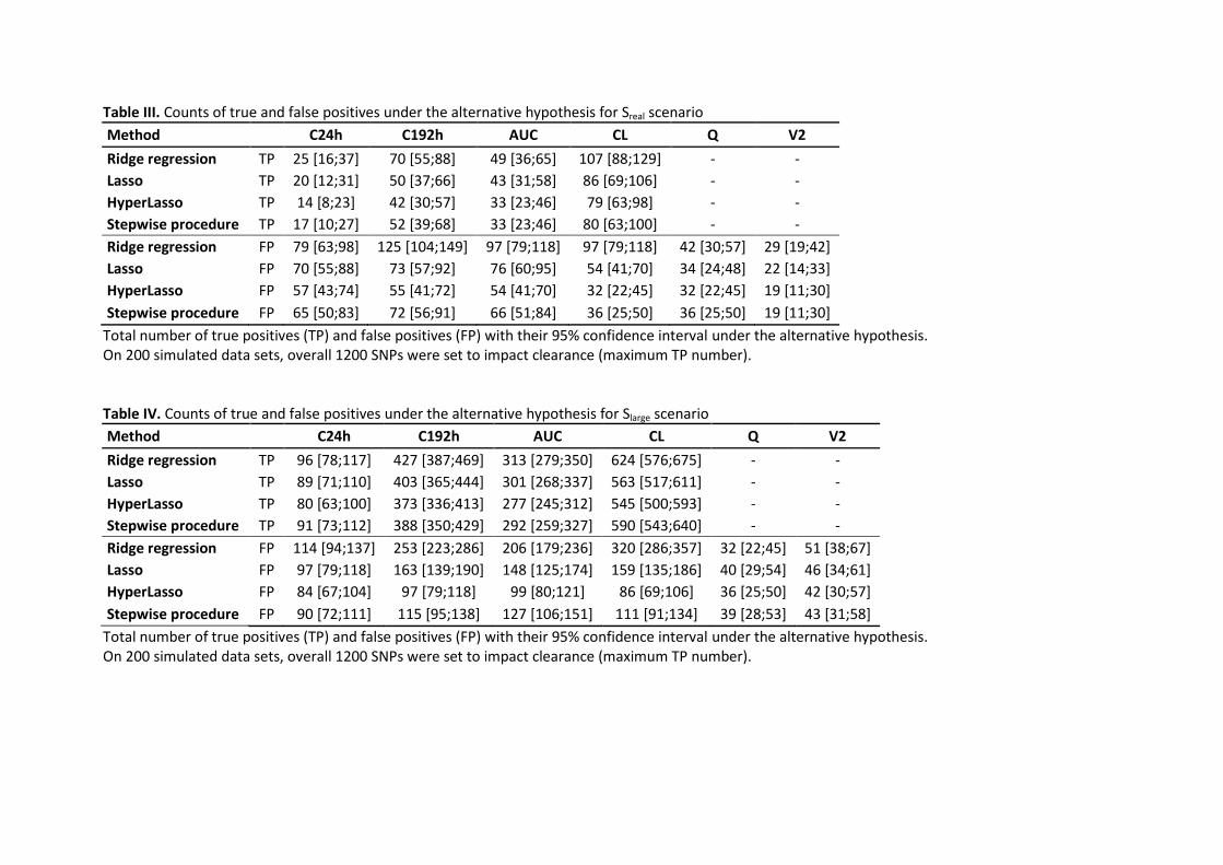
Table III. Counts of true and false positives under the alternative hypothesis for Sreal scenario

Method C24h C192h AUC CL Q V2

Ridge regression TP 25 [16;37] 70 [55;88] 49 [36;65] 107 [88;129] - -

Lasso TP 20 [12;31] 50 [37;66] 43 [31;58] 86 [69;106] - -

HyperLasso TP 14 [8;23] 42 [30;57] 33 [23;46] 79 [63;98] - -

Stepwise procedure TP 17 [10;27] 52 [39;68] 33 [23;46] 80 [63;100] - -

Ridge regression FP 79 [63;98] 125 [104;149] 97 [79;118] 97 [79;118] 42 [30;57] 29 [19;42]

Lasso FP 70 [55;88] 73 [57;92] 76 [60;95] 54 [41;70] 34 [24;48] 22 [14;33]

HyperLasso FP 57 [43;74] 55 [41;72] 54 [41;70] 32 [22;45] 32 [22;45] 19 [11;30]

Stepwise procedure FP 65 [50;83] 72 [56;91] 66 [51;84] 36 [25;50] 36 [25;50] 19 [11;30]

Total number of true positives (TP) and false positives (FP) with their 95% confidence interval under the alternative hypothesis. On 200 simulated data sets, overall 1200 SNPs were set to impact clearance (maximum TP number). Table IV. Counts of true and false positives under the alternative hypothesis for Slarge scenario

Method C24h C192h AUC CL Q V2

Ridge regression TP 96 [78;117] 427 [387;469] 313 [279;350] 624 [576;675] - -

Lasso TP 89 [71;110] 403 [365;444] 301 [268;337] 563 [517;611] - -

HyperLasso TP 80 [63;100] 373 [336;413] 277 [245;312] 545 [500;593] - -

Stepwise procedure TP 91 [73;112] 388 [350;429] 292 [259;327] 590 [543;640] - -

Ridge regression FP 114 [94;137] 253 [223;286] 206 [179;236] 320 [286;357] 32 [22;45] 51 [38;67]

Lasso FP 97 [79;118] 163 [139;190] 148 [125;174] 159 [135;186] 40 [29;54] 46 [34;61]

HyperLasso FP 84 [67;104] 97 [79;118] 99 [80;121] 86 [69;106] 36 [25;50] 42 [30;57]

Stepwise procedure FP 90 [72;111] 115 [95;138] 127 [106;151] 111 [91;134] 39 [28;53] 43 [31;58]

Total number of true positives (TP) and false positives (FP) with their 95% confidence interval under the alternative hypothesis. On 200 simulated data sets, overall 1200 SNPs were set to impact clearance (maximum TP number).

Fig. 1. Structural PK model of drug S. Double absorption compartments in red and disposition compartments in blue

Fig. 2. Stepwise procedure algorithm, adapted from Lehr et al. (24)

V1 V2 Q

FRAC × F × DOSE (1-FRAC) × F × DOSE

CL

Tk0, Tlag1 Ka, Tlag

2

Linear regressions on PK phenotype

Wald test

SNPs with significant p?

SNPs correlated (r²>0.8)?

Keep the most significant

Keep most significant SNP into final linear model

SNP left?

Final linear model

yes

no

yes

yes no

no

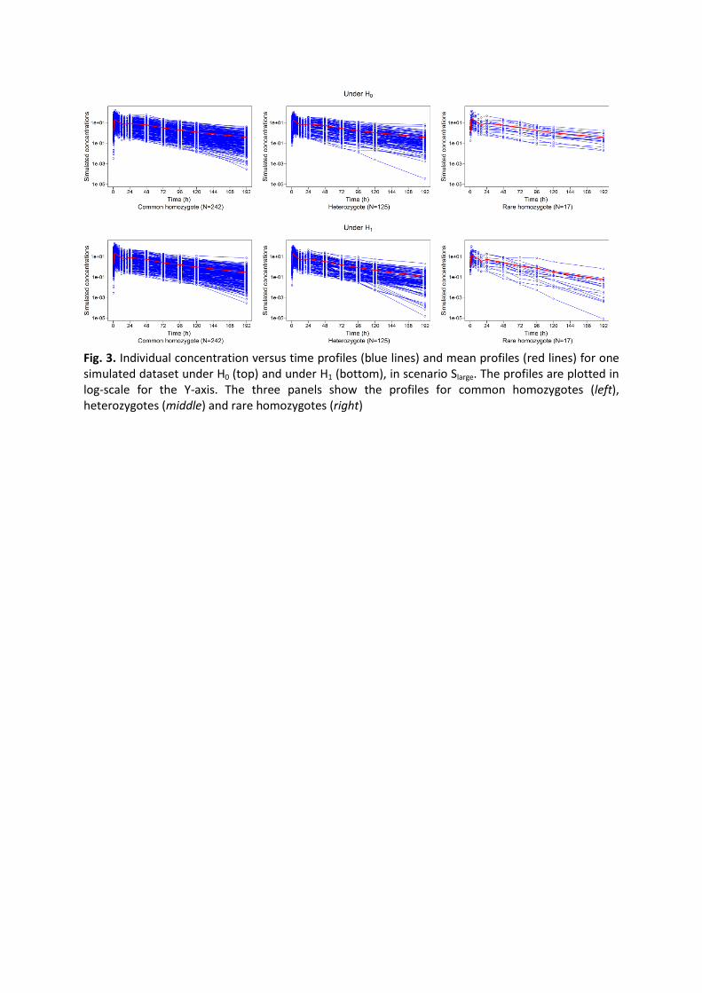
Fig. 3. Individual concentration versus time profiles (blue lines) and mean profiles (red lines) for one simulated dataset under H0 (top) and under H1 (bottom), in scenario Slarge. The profiles are plotted in log-scale for the Y-axis. The three panels show the profiles for common homozygotes (left), heterozygotes (middle) and rare homozygotes (right)

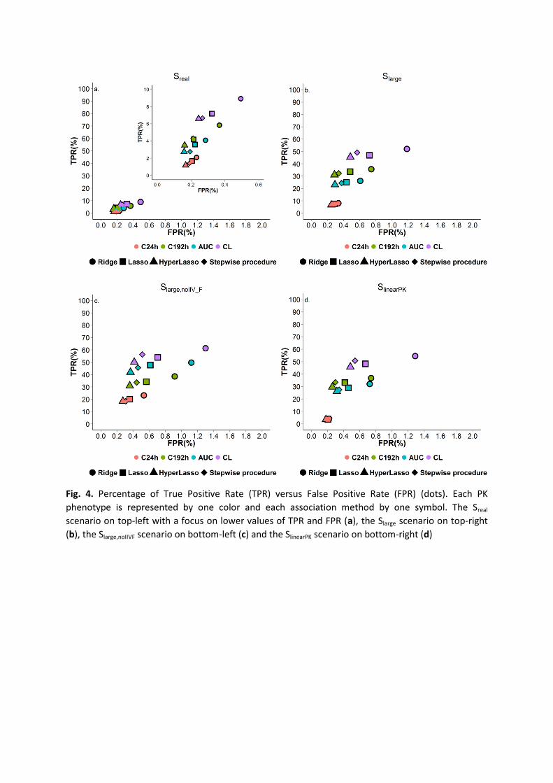
Fig. 4. Percentage of True Positive Rate (TPR) versus False Positive Rate (FPR) (dots). Each PK

phenotype is represented by one color and each association method by one symbol. The Sreal

scenario on top-left with a focus on lower values of TPR and FPR (a), the Slarge scenario on top-right

(b), the Slarge,noIIVF scenario on bottom-left (c) and the SlinearPK scenario on bottom-right (d)

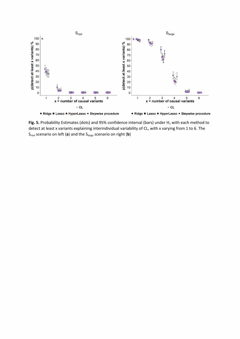
Fig. 5. Probability Estimates (dots) and 95% confidence interval (bars) under H1 with each method to

detect at least x variants explaining interindividual variability of CL, with x varying from 1 to 6. The

Sreal scenario on left (a) and the Slarge scenario on right (b)