Lecture 1: Introduction to Mixed Models with Applications ... · Lecture 1: Introduction to Mixed Models with Applications in Medicine Data with simple cluster structure Data with

Lecture 1: Introduction to Mixed Models with Applications in Medicine

Lecture 1: Introduction to Mixed Modelswith Applications in Medicine

Dankmar Bohning

Southampton Statistical Sciences Research InstituteUniversity of Southampton, UK

S3RI, 12-13 June 2014

1 / 26


Data with simple cluster structure

Testing random effects

Mixed modelling in STATA

Reliability

2 / 26




consider the following study data:

I interest is in the amount of impurity in a pharmaceuticalproduct

I data arise in form of batches of material as they come off theproduction line

I 6 batches are randomly selected

I 4 determinations are made per batch

3 / 26



Data:

impurity (in%)

Batch 1 2 3 4

1 3.28 3.09 3.03 3.072 3.52 3.48 3.38 3.433 2.91 2.80 2.76 2.854 3.34 3.38 3.23 3.315 3.28 3.14 3.25 3.216 2.98 3.01 3.13 2.95

4 / 26



questions of interest

I to determine the average amount of impurity

I batch effect?

I how large is variation between batches ?

5 / 26



ONEWAY fixed effect model

Yij = µ + βi + εij

I i = 1, · · · , 6, j = 1, · · · , 4

I βi unknown fixed parameters,∑

i βi = 0

I random error εij ∼ N(0, σ2)

I

E (Yij) = µ + βi

6 / 26



Problems with the ONEWAY fixed effect model

I number of parameters increases with the number of batches

I interest is not in a specific effect but more in a general batcheffect

I model assumes independence of observations within batches

I variance of observations is determined by variance of errors

Var(Yij) = Var(εij) = σ2

and might likely underestimate variance

I hence confidence intervals for average impurity amount mightbe too small

7 / 26



more suitable is the ONEWAY random effects model

Yij = µ + αi + εij

I i = 1, · · · , 6, j = 1, · · · , 4

I αi ∼ N(0, σ2B) are random effects


I αi and εij independent

I

E (Yij) = µ

8 / 26



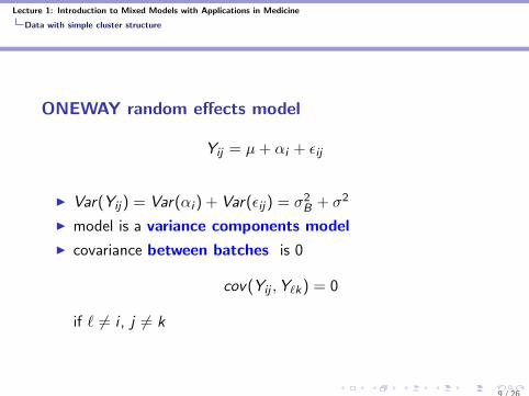
ONEWAY random effects model


I Var(Yij) = Var(αi ) + Var(εij) = σ2B + σ2

I model is a variance components model

I covariance between batches is 0

cov(Yij ,Y`k) = 0

if ` 6= i , j 6= k

9 / 26



ONEWAY random effects model


I covariance within batches is not 0 (j 6= k):

cov(Yij ,Yik) = E (α2i ) + E (αiεij) + E (αiεik) + E (εikεij) = σ2

B

I hence random effects model is suitable to model withinbatches correlation (autocorrelation model)

10 / 26






Reliability

11 / 26



ONEWAY random effects modelrandom effects


fixed effectsYij = µ + βi + εij

I fixed effects models has as many parameters βi as there arelevels of the factor

I potentially many parameters

I random effects model has only one parameter σ2B

12 / 26



Testing the random effect

random effectsYij = µ + αi + εij

how can we test the significance of a random effect?

Var(Yij) = σ2 + σ2B

I test if σ2B = 0

H0 : σ2B = 0

vs.H1 : σ2

B > 0

13 / 26



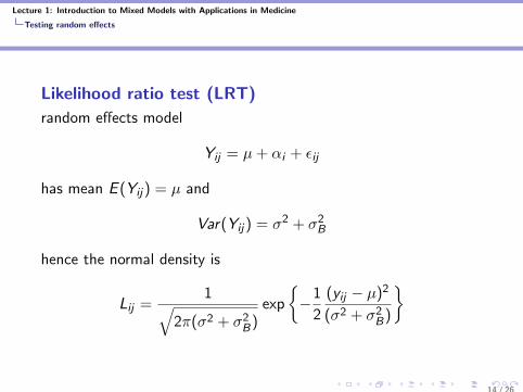
Likelihood ratio test (LRT)

random effects model


has mean E (Yij) = µ and

Var(Yij) = σ2 + σ2B

hence the normal density is

Lij =1√

2π(σ2 + σ2B)

exp

{−1

2

(yij − µ)2

(σ2 + σ2B)

}

14 / 26



Likelihood ratio test (LRT)

the full sample log-likelihood becomes

log L =∑

i

∑j

log Lij

and the likelihood ratio test becomes

2 log λ = 2(log L1 − log L0)

where the index refers to the value of σ2B under the hypothesis

(σ2B = 0 for H0 and σ2

B > 0 for H1)

2 log λ is evaluated on a χ2 scalemore precisely, 2 log λ is distributed under H0 as 0.5χ2

0 + 0.5χ21

15 / 26






Reliability

16 / 26



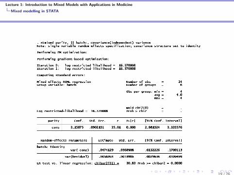
ONEWAY random effects model in STATA

I use multi-level mixed-effects linear regression module inSTATA

I specify dependent variable (Yij)

I specific random effect(s)

I change under reporting to variances and covariances

17 / 26



18 / 26



19 / 26



Important information from STATA output

I overall estimate of mean µ is 3.16 with 95% CI: 2.98–3.34

I estimate of random error variance σ2 = 0.0057

I estimate of random effect (batch) variance σ2B = 0.0474

I likelihood ratio test 2 log λ = 30.83 with p-value 0.0000(highly significant)

20 / 26






Reliability

21 / 26


Reliability

Reliability analysis

I often interest is in determining the reliability of ameasurement device (instrument, questionnaire,...)

I this means to investigate how reliable the measurementprocess is

I or how well measurements can be reproduced if the process isrepeated

I for this purpose several measurements are taken for each unit

22 / 26


Reliability

A case study

I in a microbiological experiment the number of colonies (onlog-scale) of the E. coli 0157:H7 pathogen in contaminatedfecal samples from 12 beef carcasses were determined

I two repeated measurements were taken from each of the 12carcasses for a new test (Petrifilm HEC) and a standard test

23 / 26


Reliability

Data:

carcass colonSta colonNew carcass colonSta colonNew

1 2.356 2.283 7 2.322 2.4911 2.384 2.265 7 2.491 2.4912 2.149 2.061 8 2.322 2.0412 2.263 1.987 8 2.041 2.0413 2.452 2.322 9 2.491 2.3223 2.417 2.316 9 2.322 2.0414 2.255 2.162 10 2.322 2.4914 2.299 2.127 10 2.322 2.7105 2.694 2.068 11 2.322 2.0415 2.684 2.111 11 2.491 2.3226 2.430 2.322 12 2.491 2.7856 2.440 2.280 12 2.785 2.322

24 / 26


Reliability

ONEWAY random effects model for reliability analysis


I i = 1, · · · , 12, j = 1, 2

I αi ∼ N(0, σ2B) are random effects (beef carcass)


I αi and εij independent

I

Var(Yij) = σ2B + σ2

I clearly, the larger σ2B relative to σ2, the higher the

reliability

25 / 26


Reliability

Analysis of study data:

test σ2B σ2 reliability σ2

B/(σ2B + σ2)

standard 0.0172 0.0112 0.6055new test 0.0291 0.0180 0.6183

26 / 26

Documents

Lecture 1: Introduction to Mixed Models with Applications ... · Lecture 1: Introduction to Mixed Models with Applications in Medicine Data with simple cluster structure Data with