1

PharmaSUG2010- Paper SP07

Linear Mixed Models in Clinical Trials using PROC M IXED

Danyang Bing, ICON Clinical Research, Redwood City, CA Xiaomin He, ICON Clinical Research, North Wales, PA

ABSTRACT

This paper mainly illustrates how to use PROC MIXED to fit linear mixed models in clinical trials. We first introduce the statistical background of linear mixed models. We explore the situations under which the mixed effects are identified. A randomized complete block design is used to explain the difference between PROC GLM and PROC MIXED in dealing with the linear mixed models. Examples include applications of PROC MIXED in four commonly seen clinical trials utilizing split-plot designs, cross-over designs, repeated measures analysis and multilevel hierarchical models.

KEY WORDS

Randomized complete block designs, split-plot designs, cross-over designs, repeated measures analysis, multilevel hierarchical models.

BACKGROUND AND TERMINOLOGY

During the past years, the use of linear mixed model methodology has expanded to pharmaceutical statistical areas. Many practitioners and researchers generally have taken some courses; however, many people analyzing linear mixed model data still have questions about the appropriate implementation of the methodology. Also, users who studied the topic awhile back may not be aware of the new capabilities available for applications of linear mixed models. This paper focuses on the applications of PROC MIXED with examples from commonly seen clinical trials.

The linear mixed models, also called linear mixed effects models, have two main characters:

• Models are linear in their parameters. That is, a quadratic or a higher polynomial in predictors such as

L++++ 33

2210 XXX ββββ doesn’t eliminate the curvature of plot of the response versus of the predictor. In

addition, the response value is continuous instead of categorical. Non-linear models or generalized linear models are beyond the scope of this paper.

• Mixed implies that models contain both fixed effects and random effects. Fixed effects only models or random effects only models are special cases of mixed effects models. We assume all models mentioned in this paper have both fixed effects and random effects.

In a statistical model, Littell et al (2006) define a parameter or factor to have fixed effects if the levels in the model represent all possible levels of the parameter, or at least all levels about which inference is to be made, while a parameter or factor is defined to be having random effects if the levels in the model represent only a sample (ideally, a random sample) of a larger set of potential levels. By this definition, we will always consider treatment effects as fixed because the treatments in a clinical trial are the only ones to which inference is to be made. Examples of random effect parameters or factors include:

• Block effects. Blocking is a research technique with a long history of application in experimental designs. In a typical agricultural experiment, the growth of corps with different treatments was investigated on various soils and each soil generally had all levels of treatments. Blocks of soil are used to diminish the effects of variation among corps. Similarly, in a clinical trial, treatments are always randomly assigned to units with a block, such as gender, race or some baseline characteristics (smoking versus non-smoking). That is, blocks are groups of experimental units that are formed as homogeneous as possible.

• Other model stratification effects. In a multi-center clinical trial, clinical centers or hospitals or physicians are generally added in the analysis models as one of the main or stratification effects. In a sense, a clinical center is similar to the block effect in agricultural experiments.

• Experimental units if repeated measures are applied. One example of repeated measures is in a longitudinal study in which experimental units, generally people or animals, are measured repeatedly over time. Another example of repeated measures is multilevel hierarchical models in which experimental units have two or more levels. For

2

example, in a developmental and reproductive toxicity study in rats, entire litter (or dam) and individual fetus (or pup) are usually the two levels of experimental units. In this sense, the individual fetus measures could be treated as repeatedly within the entire litter.

All of the above examples indicate that the collection data within the random effect parameter are correlated. This generic term embraces a multitude of data structure. The advantage of using linear mixed models is its ability to account for various sources of variability. If the random effect of a parameter couldn’t be correctly identified, the analysis might be lack of precision by ignoring the variability of within parameter. In some basic statistical textbooks or previous practice, random effects have been treated in the fixed effects way, or data were analyzed in multivariate regression and multivariate analysis of variance, such as in PROC GLM. PROC MIXED provides more flexibility and precisions than PROC GLM in lots of areas such as identifying the variance-covariance matrix. We will discuss it in the later section.

Littell et al. (2006) are also aware of the controversies of deciding whether a parameter or factor is random or fixed. The block effect is a good example. In the modern clinical trials, the block parameter is generally composed of all possible levels. For example, gender will include both males and females. Baseline dichotomous parameters with a flag of “yes” or “no” contain all possibilities. Some study may have age group as “18<-40”, “40<-60” and “60 or above”. If the inclusion/exclusion criteria specify only subject above 18 years of age are allowed to be enrolled, then the age block could be still treated as containing all levels of interested to the study. In this sense, most of block effects in a clinical trial are fixed and will be added in the model for one of the main effects if needed. A randomized blocks design example in the later section illustrates when the block is random in an experimental design.

Treating stratification effects as fixed or random is another controversy. We use clinical center as a stratification example. Depending on the effect on the overall treatment from the stratification factors, Mehrotra (2001) divides them as prognostic and non-prognostic factors. Prognostic factors are known to influence the response variables in a systematic way, while non-prognostic factors are likely to impact the trial’s response but their effects do not exhibit a predictable pattern. In this sense, clinical centers influence the overall treatment effect in a fairly random manner and it is natural to classify the center as a non-prognostic factor. Dmitrienko et al. (2006) mention “Even though most of the discussion on center effects in the ICH guidance document ‘Statistical principles for clinical trials’ (ICH E9) treats center as a fixed effect, the guidance also encourages trialists to explore the heterogeneity of the treatment effect across centers using mixed models.”

In any cases, if there are repeated measures within an experimental unit, the experimental unit will be treated as random and the linear mixed model will be utilized.

AN INTRODUCTION: RANDOMIZED COMPLETE BLOCK DESIGN ( RCBD)

A randomized blocks design that has each treatment applied to an experimental unit in each block is called a randomized complete blocks design (RCBD). Assume there are t treatments and r blocks in a clinical trial. Also assume there are s independent experimental units per each treatment and block; so there are a total of trs experimental units. Denote ijkY by

the response from the kth experimental unit receiving treatment i in block j .

The equation for the model is

ijkjiijk ebY +++= τµ , where ti ,...,2,1= , rj ,...,2,1= and sk ,...,2,1= .

In this model:

• µ is the intercept of the model, which is always assumed to be a fixed parameter; • iτ is the fixed effect parameter for ith treatment;

• jb is the random effect associated with the jth block, and jb ’s are identically and independent distributed (iid)

as ( )2,0 bN σ for rj ,...,2,1= ;

• ijke is the random error associated with the kth experimental unit receiving treatment i in block j , and ijke ’s are iid

as ( )2,0 σN for ti ,...,2,1= , rj ,...,2,1= and sk ,...,2,1= ; • jb and ijke are also independent for ti ,...,2,1= , rj ,...,2,1= and sk ,...,2,1= .

The data are balanced because the number of experimental units with each treatment i and block j is identical. In some situations each treatment appears once in each block, so the subscript of k could be removed from the equation. In the most common situations, the number of experimental units may vary with each treatment i and block j such as ijnk ,...,2,1= .

PROC MIXED can analyze an unbalanced data in the same way as the balanced data, but it will provide more accurate results than PROC GLM.

3

Example 1: Soil Type Data (Stenstrom, 1940)

Stenstrom (1940) designs an experiment to investigate how snapdragons grow in 6 different soil types. To eliminate the effect of local fertility variations, the experiment is run in 3 blocks, with each soil type sampled in each block. This example is used to illustrate data analysis using Randomized Complete Block Design and Randomized Incomplete Block Design.

COMPLETE BLOCK DESIGN

Statements for PROC GLM and PROC MIXED for RCBD using soil type data are:

PROC GLM DATA=PLANTS; CLASS BLOCK TYPE; MODEL STEMLENGTH = BLOCK TYPE; RANDOM BLOCK; ODS SELECT OVERALLANOVA MODELANOVA; RUN; PROC MIXED DATA=PLANTS COVTEST; CLASS BLOCK TYPE; MODEL STEMLENGTH = TYPE; RANDOM BLOCK; ODS SELECT COVPARMS TESTS3; RUN; The class statement defines both BLOCK and TYPE as class variables. In the model statement, left hand side of equation sign is the response variable, which is STEMLENGTH in this example, while the variables on the right hand side are the fixed effects. Comparing the statements for PROC GLM and PROC MIXED, note the random effect BLOCK is in the model statement in PROC GLM, but not included in the model statement in PROC MIXED. Since BLOCK is in the model statement in PROC GLM, PROC GLM ANOVA table list BLOCK as fixed effect together with TYPE, as you can see from output 1.1. PROC MIXED only summarizes fixed effect TYPE in the model, see output 1.2. Random effect is specified in RANDOM statement. ODS statement from PROC GLM outputs overall ANOVA results and model ANOVA results. ODS statement from PROC MIXED outputs Covariance Parameter Estimate and fixed effect (TYPE 3) results. Results from these statements are displayed in Output 1.1 and Output 1.2. Output 1.1 Complete Block Analysis with PROC GLM

Linear Mixed Model using PROC GLM

Sum of

Source DF Squares Mean Square F Value Pr > F

Model 8 142.1885714 17.7735714 10.80 0.0002

Error 12 19.7428571 1.6452381

Corrected Total 20 161.9314286

Source DF Type I SS Mean Square F Value Pr > F

Block 2 39.0371429 19.5185714 11.86 0.0014

Type 6 103.1514286 17.1919048 10.45 0.0004

Source DF Type III SS Mean Square F Value Pr > F

Block 2 39.0371429 19.5185714 11.86 0.0014

Type 6 103.1514286 17.1919048 10.45 0.0004 Output 1.2 Complete Block Analysis with PROC MIXED

Linear Mixed Model using PROC MIXED

Covariance Parameter Estimates

standard Z

Cov Parm Estimate Error Value Pr Z

Block 2.5533 2.7900 0.92 0.1801

Residual 1.6452 0.6717 2.45 0.0072

Type 3 Tests of Fixed Effects

Num Den

Effect DF DF F Value Pr > F

Type 6 12 10.45 0.0004

4

The basic computation for PROC GLM is analysis of variance, while PROC MIXE is based on restricted maximum likelihood estimation. From PROC GLM output 1.1, both BLOCK and TYPE are summarized in ANOVA table. Because these data are balanced, the Type I and Type III Sum of Squares are the same. In PROC MIXED output 1.2, “Type 3 Tests of Fixed Effects” table contains the fixed type effect only and it gives numerator and denominator degree of freedom but not the sum of squares. Results and conclusions using PROC GLM and PROC MIXED are essentially the same for fixed effect TYPE (0.0004) and overall error estimate (1.645), because the data are complete and balanced. The variability of within-block could be correctly estimated in fixed block effect. As you may notice, the results for random effect BLOCK is not same from PROC GLM (0.0014) and PROC MIXED (0.1801) due to different algorithm used in PROC GLM vs. PROC MIXED.

INCOMPLETE BLOCK DESIGN

For the purpose of illustration of Incomplete Block Design, we randomly impute some measures as missing to make the data “unbalanced” to compare PROC GLM and PROC MIXED for Incomplete Block Analysis.

Output 1.3 Incomplete Block Analysis with PROC GLM

Linear Mixed Model using PROC GLM

Sum of

Source DF Squares Mean Square F Value Pr > F

Model 8 133.6637879 16.7079735 8.68 0.0020

Error 9 17.3212121 1.9245791

Corrected Total 17 150.9850000

Source DF Type I SS Mean Square F Value Pr > F

Block 2 34.54333333 17.27166667 8.97 0.0072

Type 6 99.12045455 16.52007576 8.58 0.0026

Source DF Type III SS Mean Square F Value Pr > F

Block 2 37.85212121 18.92606061 9.83 0.0054

Type 6 99.12045455 16.52007576 8.58 0.0026

Output 1.4 Incomplete Block Analysis with PROC MIXED

Linear Mixed Model using PROC MIXED

Covariance Parameter Estimates

Standard Z

Cov Parm Estimate Error Value Pr Z

Block 3.0912 3.4451 0.90 0.1848

Residual 1.9246 0.9073 2.12 0.0169

Type 3 Tests of Fixed Effects

Num Den

Effect DF DF F Value Pr > F

Type 6 9 8.53 0.0027

Type I and Type III Sum of Squares in PROC GLM are not the same due to the unbalanced data. In this case, results of Type III Sum of Squares would be recommended. Generally, the p-value by linear mixed model using PROC MIXED is smaller than the p-value by linear mixed model using PROC GLM, because the former combined within- and between-block estimates of the type effect. This example didn’t show so due to the sparse data.

5

CLINICAL TRIAL APPLICATION

SPLIT-PLOT DESIGN

One of the most common clinical trials is the split-plot design. The split-plot design involves two experimental factors, A and B. Levels of A are randomly assigned to whole plots (main plots), and levels of B are randomly assigned to split plots (subplots) within each whole plot. The subplots are assumed to be nested within the whole plots so that a whole plot consists of a cluster of subplots and a level of A is applied to the entire cluster. The design provides more precise information about B than about A, and it often arises when A can be applied only to large experimental units. Split plot studies are often used to improve the precision of the estimated effects of the factor applied to the subunits.

Multi-location trial example is used to illustrate split plot design. The objectives of using multi-location trials are comparing treatments averaged over the entire population represented by locations (main plot effects) and estimating treatment-by-location interaction (sub-plot effects). Significant sub-plot effects may imply needs for location-specific treatment recommendations.

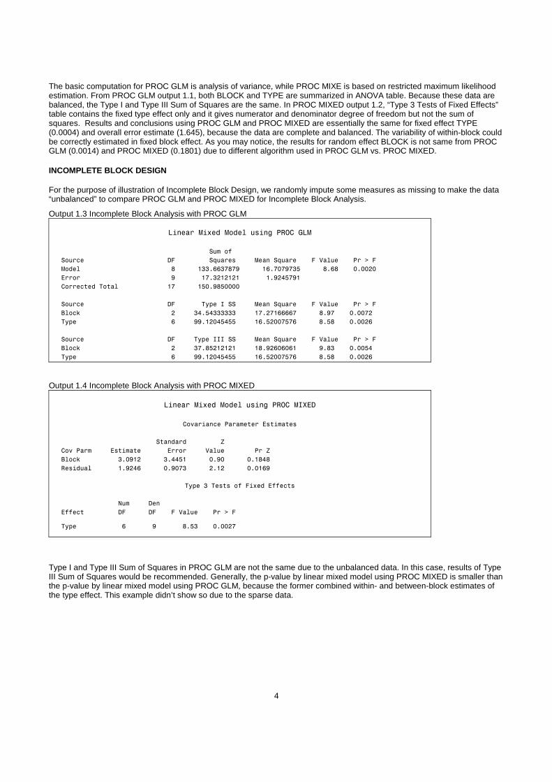
Example 2: Multi-location Trial (Littell et al 2006)

In this example, 4 treatments were observed at each of 9 locations. At each location, a randomized complete block design with 3 blocks was used. The equation for this model is

ijklijjkjiijkl eLLRLY +++++= )()( ττµ

In this model: • µ is the intercept of the model;

• iτ is the ith fixed treatment, 1=i ,2,3,4;

• jL is the jth location, j=1,…,9;

• jkLR )( is the random effect of block k within location L, 3,2,1=k

• ijL)(τ is the treatment by location interaction

• ijkle is the random error associated with the lth subject receiving treatment i in location j , and within kth block;

Both block within location effect jkLR )( and error effect ijkle are assumed random and independent of each other.

Figure 2.1: Plot for multi-location data by Locations/blocks and Treatments

6

SAS statements using PROC MIXED for this analysis are followed, results are in output 2.1. PROC MIXED DATA=MUL COVTEST; CLASS LOC BLOCK TRT; MODEL ADG=LOC TRT LOC*TRT; RANDOM BLOCK(LOC); RUN;

PROC MIXED statement COVTEST option requests significance tests for the random effects. The class statement defines LOC, BLOCK, and TRT as class variable. The model statement defines LOC, TRT, as well as location and treatment interaction LOC*TRT as fixed effect. The random statement specifies blocks within location as random effect. Results are shown in output 2.1.

OUTPUT 2.1 Split-plot Analysis for multi-location data from PROC MIXED

PROC MIXED Procedure

Covariance Parameter Estimates

Standard Z

Cov Parm Estimate Error Value Pr Z

block(loc) 0.005620 0.005038 1.12 0.1323

RESIDUAL 0.03458 0.006655 5.20 <.0001

Type 3 Tests of Fixed Effects

Num Den

Effect DF DF F Value Pr > F

loc 8 18 25.11 <.0001

trt 3 54 11.78 <.0001

loc*trt 24 54 1.20 0.2829

From output 2.1 covariance parameter estimate, block within location variance estimate is 0.005620, it does not have significant effect with p=0.1323. Residual estimate is 0.03458 with p-value 0.0001. By default, PROC MIXED uses TYPE=VC (variance components) in the random statement which assumes the zero covariance among each variance. Fixed effects results show both location and treatment are statistically significant, but location by treatment interaction effect is not significant.

CROSS-OVER DESIGN

Cross-over design is another very often used study design used in clinical trials. In the design, subjects receive all treatments in sequence. Each subject serves as his/her own control, in contrast with parallel group design where each group gets different treatments. Since same subject receives both treatments, this analysis can avoid possibility of covariate imbalance. Typically in cross-over design, each subject is randomly assigned to a specific treatment order. Some subjects receive standard therapy first, followed by the new therapy. Others receive the new therapy first, followed by the standard therapy. A common approach in cross-over study is to test carry-over effect. Carry-over effect is that treatment effect in the previous period is “carried over” to the later period, which is very likely to happen in cross-over study. If carry-over effect is observed, common solution for carry-over effect can be minimized by adding a wash-out period between the periods using different treatments.

Example 3: COPD Data (Jones & Kenward, 2003)

These are data from a placebo-controlled, double-blind randomized study to evaluate the efficacy and safety of an inhaled drug given twice daily via an inhaler in patients with chronic obstructive pulmonary disease (COPD). Eligible patients were randomized to receive drug (A) or matching placebo (B) for 4 weeks, and then switched over to the alternative treatment for a further 4 weeks. Patients will be in the sequence of either AB or BA. There are 27 in AB sequence and 29 in the BA sequence. The primary endpoint is the mean morning expiratory flow rate (PEFR, L/min).

The equation for the model is

ijklklijkijkl ebsY +++++= )(τπµ , where 2,1=i , 2,1=j , 2,1=k and knl ,...,2,1= .

In this model:

7

• µ is the intercept of the model; • iτ is the ith fixed treatment, 1=i (drug A) or 2= (placebo);

• jπ is the jth fixed period, 1=j (period 1) or 2= (period 2);

• ks is the kth fixed sequence, 1=k (sequence AB) or 2= (sequence BA);

• ( )klb is the random patient effect associated with the lth subject within kth sequence;

• ijkle is the random error associated with the lth subject receiving treatment i in period j , and within kth sequence;

• ( )klb and ijkle are independent for 2,1=i , 2,1=j , 2,1=k and knl ,...,2,1= .

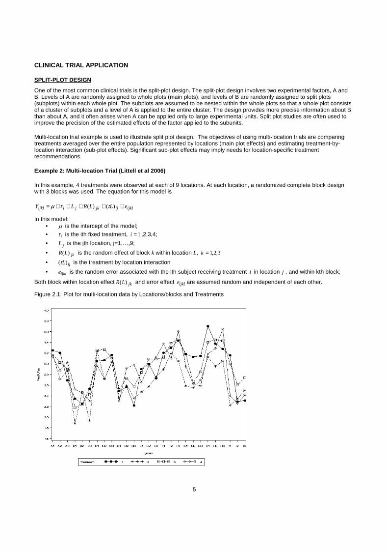
Figure 3.1: Mean and standard errors for mean morning expiratory flow rate by Period and Sequence

Figure 3.1 plots the mean and standard errors for Mean Morning Expiratory Rate by period and sequence. Subjects on Sequence 1 had treatment A at period 1 and treatment B at period 2. Subjects on sequence 2 had treatment B at period 1 and treatment A at period 2. This plots shows treatment A (sequence 1 at period 1 and sequence 2 at period 2) leads to consistent higher rate and treatment B (sequence 1 at period 2 and sequence 2 at period 1) results in lower rate. SAS statements using PROC MIXED for this analysis are follows, results are in output 3.1.

PROC MIXED DATA=COPD; CLASS PATIENT SEQUENCE PERIOD TREAT; MODEL RESPONSE = SEQUENCE PERIOD TREAT; RANDOM PATIENT(SEQUENCE); LSMEANS TREAT/ PDIFF; RUN;

The model statement defines SEQUENCE, PERIOD and TREAT as fixed effects. The random statement specifies sequence within patient as random effect. LSMEANS requests mean square estimate for each treatment. PDIFF options gives t-test results for comparing the mean square estimates for the 2 treatments. Estimate statement again gives results for comparing DRUG A to PLACEBO. Results are shown in output 3.1. In this study, the sources of variation have two: one is from between-subjects and the other is from within-subjects. The between-subject variation includes a carry-over treatment effect and between-subject residuals. The carry-over treatment effect was often seen and being testing in a cross-over study. That is, the investigator needs ensure in Sequence 1, drug A treatment effect in the first period shouldn’t be carried out to the second period; and on the other hand, in Sequence 2, placebo effect in the first period shouldn’t also be carried to the second period. By the results, the observed p-value at sequence parameter (p=0.3472) indicates the carry-over treatment effect is statistically insignificant. The within-subject variation includes direct treatment effect, period effect, and within-subject residuals. The direct treatment effect is of our interest, and its observed p-value at 0.0036 is strong evidence of existence of treatment. Since the observed p-value at 0.2749 is insignificant for period, we would also claim there is no “cross-over” period effect in the data. We also use ESTIMATE statement in PROC MIXED procedure to explore the treatment difference between drug (A) and placebo (B) adjusted for carry-over and period effect, which is equivalent to the Type 3 test results of fixed effects.

A

B

A

B

8

Output 3.1 Cross-Over Analysis for COPD data from PROC MIXED

PROC MIXED Procedure

Covariance Parameter Estimates

Cov Parm Estimate

patient(sequence) 5715.26

Residual 326.24

Type 3 Tests of Fixed Effects

Num Den

Effect DF DF F Value Pr > F

sequence 1 54 0.90 0.3472

period 1 54 1.22 0.2749

treat 1 54 9.28 0.0036

Least Squares Means

Standard

Effect treat Estimate Error DF t Value Pr > |t|

treat 1 227.60 10.3934 54 21.90 <.0001

treat 2 238.00 10.3934 54 22.90 <.0001

Differences of Least Squares Means

Standard

Effect treat _treat Estimate Error DF t Value Pr > |t|

treat 1 2 -10.4026 3.4156 54 -3.05 0.0036

REPEATED MEASURES DESIGN

In practice, longitudinal data are often highly unbalanced in the sense that not an equal number of measurements are available for all subjects and/or that measurements are not taken at fixed time points. Due to their unbalanced nature, many longitudinal data sets cannot be analyzed using multivariate regression techniques. A natural alternative arises from observing that subject-specific longitudinal profiles can often be well approximated by linear regression functions.

Example 4 Lecithin in treatment of Alzheimer’s dise ase (Der & Everitt, 2002)

A study for the use of Lecithin in the treatment of Alzheimer’s disease was used to illustrate this study design. Recent work suggests that Alzheimer’s disease might be possible to remedy by long-term dietary enrichment with lecithin. Patients suffering from Alzheimer’s disease were randomly allocated to receive either placebo (group=1) or Lecithin (group=2) for a 6-month periods. A cognitive test score giving the number of words recalled from a previously given standard list was recorded monthly for 5 months.

ijkkjijijkl ebY ++++= )(τπµ , where 2,1=i , 5,...,1=j , and nk ,...,1= .

In this model: • µ is the intercept of the model; • iτ is the ith fixed treatment, 1=i (placebo) or 2= (Lecithin);

• jπ is the jth fixed visit, 5,...,1=j ;

• ( )kjb is the random visit effect at the jth visit of the kth subject;

• ijke is the random error associated with the kth subject receiving treatment i at visit j ;

• ( )kjb and ijke are independent for 2,1=i , 5,...,1=j , and nk ,...,1= .

9

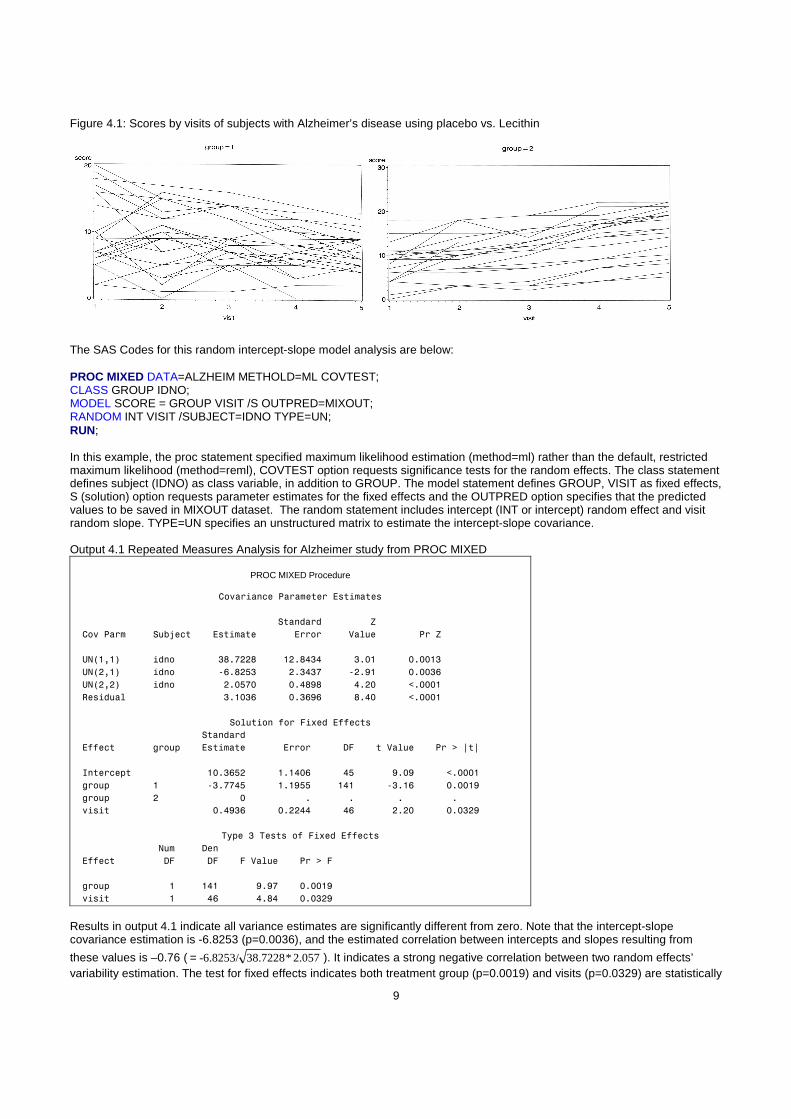
Figure 4.1: Scores by visits of subjects with Alzheimer’s disease using placebo vs. Lecithin

The SAS Codes for this random intercept-slope model analysis are below: PROC MIXED DATA=ALZHEIM METHOLD=ML COVTEST; CLASS GROUP IDNO; MODEL SCORE = GROUP VISIT /S OUTPRED=MIXOUT; RANDOM INT VISIT /SUBJECT=IDNO TYPE=UN; RUN; In this example, the proc statement specified maximum likelihood estimation (method=ml) rather than the default, restricted maximum likelihood (method=reml), COVTEST option requests significance tests for the random effects. The class statement defines subject (IDNO) as class variable, in addition to GROUP. The model statement defines GROUP, VISIT as fixed effects, S (solution) option requests parameter estimates for the fixed effects and the OUTPRED option specifies that the predicted values to be saved in MIXOUT dataset. The random statement includes intercept (INT or intercept) random effect and visit random slope. TYPE=UN specifies an unstructured matrix to estimate the intercept-slope covariance. Output 4.1 Repeated Measures Analysis for Alzheimer study from PROC MIXED

PROC MIXED Procedure

Covariance Parameter Estimates

Standard Z

Cov Parm Subject Estimate Error Value Pr Z

UN(1,1) idno 38.7228 12.8434 3.01 0.0013

UN(2,1) idno -6.8253 2.3437 -2.91 0.0036

UN(2,2) idno 2.0570 0.4898 4.20 <.0001

Residual 3.1036 0.3696 8.40 <.0001

Solution for Fixed Effects

Standard

Effect group Estimate Error DF t Value Pr > |t|

Intercept 10.3652 1.1406 45 9.09 <.0001

group 1 -3.7745 1.1955 141 -3.16 0.0019

group 2 0 . . . .

visit 0.4936 0.2244 46 2.20 0.0329

Type 3 Tests of Fixed Effects

Num Den

Effect DF DF F Value Pr > F

group 1 141 9.97 0.0019

visit 1 46 4.84 0.0329 Results in output 4.1 indicate all variance estimates are significantly different from zero. Note that the intercept-slope covariance estimation is -6.8253 (p=0.0036), and the estimated correlation between intercepts and slopes resulting from

these values is –0.76 ( 2.057*38.7228-6.8253/= ). It indicates a strong negative correlation between two random effects’ variability estimation. The test for fixed effects indicates both treatment group (p=0.0019) and visits (p=0.0329) are statistically

10

significant. The parameter estimate for group indicates that the placebo group (group 1) has a lower average cognitive score than the Lecithin group (group 2).

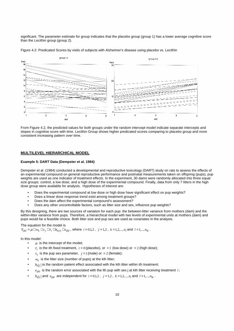
Figure 4.2: Predicated Scores by visits of subjects with Alzheimer’s disease using placebo vs. Lecithin

From Figure 4.2, the predicted values for both groups under the random intercept model indicate separate intercepts and slopes in cognitive score with time. Lecithin Group shows higher predicated scores comparing to placebo group and more consistent increasing pattern over time.

MULTILEVEL HIERARCHICAL MODEL

Example 5: DART Data (Dempster et al. 1984)

Dempster et al. (1984) conducted a developmental and reproductive toxicology (DART) study on rats to assess the effects of an experimental compound on general reproductive performance and postnatal measurements taken on offspring (pups), pup weights are used as one indicator of treatment effects. In the experiment, 30 dams were randomly allocated into three equal size groups: control, a low dose, and a high dose of the experimental compound. Finally, data from only 7 litters in the high dose group were available for analysis. Hypotheses of interest are:

• Does the experimental compound at low dose or high dose have significant effect on pup weights? • Does a linear dose response trend exist among treatment groups? • Does the dam affect the experimental compound’s assessment? • Does any other uncontrollable factors, such as litter size and sex, influence pup weights?

By this designing, there are two sources of variation for each pup: the between-litter variance from mothers (dam) and the within-litter variance from pups. Therefore, a hierarchical model with two levels of experimental units at mothers (dam) and pups would be a feasible choice. Both litter size and pup sex are used as covariates in the analysis.

The equation for the model is

ijklikijkijkl ebswY +++++= )(τµ , where 2,1,0=i , 2,1=j , ink ,...,2,1= and iknl ,...,1= .

In this model:

• µ is the intercept of the model; • iτ is the ith fixed treatment, 0=i (placebo), or 1= (low dose) or 2= (high dose);

• js is the pup sex parameter, 1=j (male) or 2= (female);

• kw is the litter size (number of pups) at the kth litter;

• ( )ikb is the random patient effect associated with the kth litter within ith treatment;

• ijkle is the random error associated with the lth pup with sex j at kth litter receiving treatment i ;

• ( )ikb and ijkle are independent for 2,1,0=i , 2,1=j , ink ,...,2,1= and iknl ,...,1= .

11

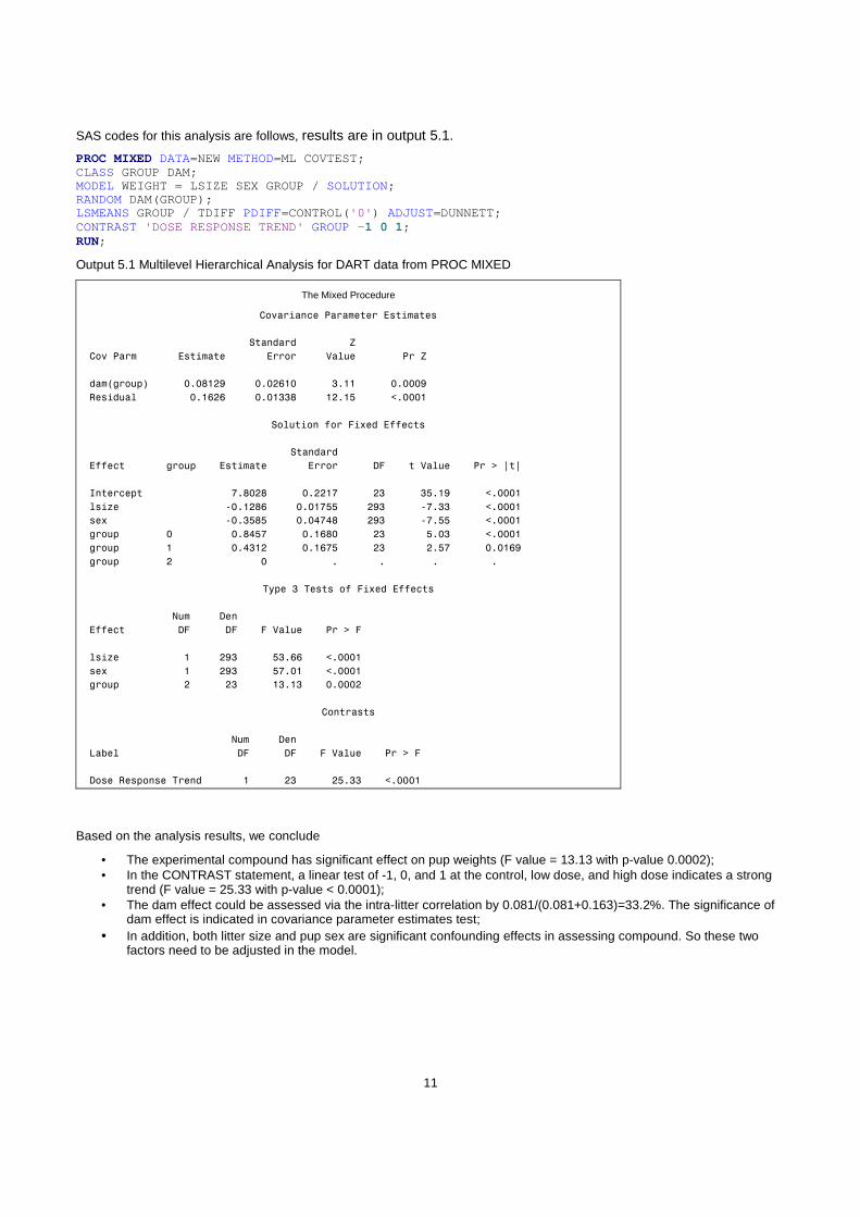
SAS codes for this analysis are follows, results are in output 5.1.

PROC MIXED DATA=NEW METHOD=ML COVTEST; CLASS GROUP DAM; MODEL WEIGHT = LSIZE SEX GROUP / SOLUTION; RANDOM DAM(GROUP); LSMEANS GROUP / TDIFF PDIFF=CONTROL('0' ) ADJUST=DUNNETT; CONTRAST 'DOSE RESPONSE TREND' GROUP - 1 0 1; RUN;

Output 5.1 Multilevel Hierarchical Analysis for DART data from PROC MIXED

The Mixed Procedure

Covariance Parameter Estimates

Standard Z

Cov Parm Estimate Error Value Pr Z

dam(group) 0.08129 0.02610 3.11 0.0009

Residual 0.1626 0.01338 12.15 <.0001

Solution for Fixed Effects

Standard

Effect group Estimate Error DF t Value Pr > |t|

Intercept 7.8028 0.2217 23 35.19 <.0001

lsize -0.1286 0.01755 293 -7.33 <.0001

sex -0.3585 0.04748 293 -7.55 <.0001

group 0 0.8457 0.1680 23 5.03 <.0001

group 1 0.4312 0.1675 23 2.57 0.0169

group 2 0 . . . .

Type 3 Tests of Fixed Effects

Num Den

Effect DF DF F Value Pr > F

lsize 1 293 53.66 <.0001

sex 1 293 57.01 <.0001

group 2 23 13.13 0.0002

Contrasts

Num Den

Label DF DF F Value Pr > F

Dose Response Trend 1 23 25.33 <.0001

Based on the analysis results, we conclude

• The experimental compound has significant effect on pup weights (F value = 13.13 with p-value 0.0002); • In the CONTRAST statement, a linear test of -1, 0, and 1 at the control, low dose, and high dose indicates a strong

trend (F value = 25.33 with p-value < 0.0001); • The dam effect could be assessed via the intra-litter correlation by 0.081/(0.081+0.163)=33.2%. The significance of

dam effect is indicated in covariance parameter estimates test; • In addition, both litter size and pup sex are significant confounding effects in assessing compound. So these two

factors need to be adjusted in the model.

12

CONCLUSION

This paper illustrates various applications of linear mixed models using PROC MIXED. Readers should be aware that the definitions of above applications are not clear-cut. For example, in the multilevel hierarchical models, the higher level of experimental unit could be treated as a random block factor, so the concept of split-plot design may apply. The paper itself doesn’t intentionally to explain whether the linear mixed models are the best choices to analyze the data or not. Methods to be used depend on the nature of data instead of software. Good statistical applications require a certain amount of theoretical knowledge. The more advanced the application, the more theoretical skills will help.

REFERENCES

SAS/STAT® 9.1.3 User’s Guide, The GLM and MIXED Procedures.

Ramon Littell, George Milliken, Walter Stroup, Russell Wolfinger, and Oliver Schabenberger. (2006). SAS for Mixed Models, Second Edition, SAS Institute Inc.

Alex Dmitrienko, Geert Molenberghs, Christy Chuang-Stein, and Walter Offen. (2005). Analysis of Clinical Trials Using SAS®: A Practical Guide. Cary, NC: SAS Institute Inc.

Mehrotra, D.V. (2001). Stratification issues with binary endpoints. Drug Information Journal, 35, 1343–1350.

Stenstrom, F. H. (1940). The Growth of Snapdragons, Stocks, Cinerarias and Carnations on Six Iowa Soils, Master's thesis, Iowa State College.

Byron Jones, and Michael G. Kenward. (2003). Design and Analysis of Cross-Over Trials. Second Edition. Chapman & Hall/CRC.

Dempster, Selwyn, Patel & Roth (1984) Statistical and Computational Aspects of Mixed Model Analysis, Applied Statistics, 33, No. 2, pp. 203-214

ACKNOWLEDGMENTS We would like to thank ICON Clinical Research for consistently encouraging and supporting conference participation, and all ICON colleagues for their support. We sincerely would like to thank Syamala Schoemperlen for her suggestions and making the participation in this year’s conference possible. CONTACT INFORMATION Your comments and questions are valued and encouraged. Contact the author at:

Name: Xiaomin He, Ph.D. Enterprise: ICON Clinical Research Address: 1700 Pennbrook Parkway City, State ZIP: North Wales, PA 19454 Work Phone: 215-616-6406 Fax: 215-616-8685 E-mail: Xiaomin.he@iconplc.com Web: www.iconplc.com

SAS and all other SAS Institute Inc. product or service names are registered trademarks or trademarks of SAS Institute Inc. in the USA and other countries. ® indicates USA registration. Other brand and product names are trademarks of their respective companies.