META-STABLE STATES OF VEGETATIVE HABITATS IN WATER

CONSERVATION AREA 3A, EVERGLADES

By

ERIK POWERS

A THESIS PRESENTED TO THE GRADUATE SCHOOL OF THE UNIVERSITY OF FLORIDA IN PARTIAL FULFILLMENT

OF THE REQUIREMENTS FOR THE DEGREE OF MASTER OF SCIENCE

UNIVERSITY OF FLORIDA

2005

Copyright 2005

by

Erik Powers

This document is dedicated to my father, Dr. Lawrence W. Powers, who inspired my fascination with science early in life.

iv

ACKNOWLEDGMENTS

I must first thank Dr. Wiley Kitchens for his unwavering support and

encouragement throughout my graduate career. I thank my committee members Dr. Paul

Wetzel and Dr. Ted Schuur for their advice and guidance. Instrumental in the

experimental design, Paul Wetzel has provided support from the beginning. Paul

Conrads of the USGS performed the neural network analysis for the hydrologic data set.

His assistance was paramount to the completion of this thesis.

Logistic support, including airboats and lodging, was provided by the Florida

Cooperative Fish and Wildlife Unit, University of Florida, Gainesville. The following

University of Florida graduate students and staff helped with field sampling and data

processing: Stephen Brooks, Janell Brush, Melissa DeSa, Jamie Duberstein, Joey

Largay, Kristianna Lindgren, Julien Martin, Ann Marie Muench, Alison Pevler, Laura

Pfenninger, Derek Piotrowicz, Zach Welch, and Christa Zweig. Lastly, I thank my wife

and best friend, Kristy Powers, for her undying patience and compassion despite my

propensity for tracking mud into the house.

v

TABLE OF CONTENTS

Page ACKNOWLEDGMENTS ................................................................................................. iv

LIST OF TABLES........................................................................................................... viii

LIST OF FIGURES ........................................................................................................... ix

ABSTRACT..................................................................................................................... xiii

CHAPTER

1 INTRODUCTION ........................................................................................................1

What Are Meta-stable States? ......................................................................................2 How Community Subtypes and Driving Forces Are Determined ................................4 Communities of the Everglades....................................................................................6 Project Objectives.........................................................................................................8

2 DETERMINING COMMUNITY STRUCTURE ........................................................9

Description of Study Site............................................................................................11 Methods and Materials ...............................................................................................14

Sampling Regime ................................................................................................14 Sampling Methodology .......................................................................................15 Processing Methodology .....................................................................................16 Data preparation and Relativization ....................................................................16

3 CLASSIFICATION OF META-STABLE STATES .................................................20

Hierarchical Agglomerative Cluster Analysis ............................................................21 Testing Importance Value Assumptions.....................................................................21 Indicator Species Analysis..........................................................................................27 Matching Similar Community Descriptions Between Sampling Events....................28 Distribution of Meta-Stable States Across the Landscape .........................................30

4 MULTIVARIATE ANALYSIS AND RESULTS .....................................................33

Hydrology ...................................................................................................................33 Selecting Hydrologic Variables...........................................................................33

vi

Calculating Hydrologic Variables .......................................................................35 Hindcasting using neural networks ..............................................................35 Extrapolating from well data to sample unit data ........................................38

Nonmetric Multidimensional Scaling.........................................................................39 Classification Trees and Characterization of Meta-Stable States by Environmental

Variables ................................................................................................................45 Slough Physiognomic Type.................................................................................46

Deep sloughs ................................................................................................47 Eleocharis elongata sloughs ........................................................................48 Panicum sloughs ..........................................................................................48 Shallow sloughs............................................................................................48

Wet Prairie Physiognomic Type..........................................................................48 Eleocharis sp. prairie...........................................................................................49

E. elongata prairie ........................................................................................50 Panicum/Paspalidium/Eleocharis prairies ...................................................50 Sawgrass prairies..........................................................................................50

Sawgrass Physiognomic Types ...........................................................................51 Sawgrass monoculture (heavy sawgrass) .....................................................51 Sawgrass with Bacopa and Ludwigia...........................................................52 Sawgrass with Eleocharis sp. and Panicum.................................................52 Sawgrass with E. elongata and Crinum .......................................................52

Island Physiognomic Types.................................................................................53 Ghost islands ................................................................................................54 Sawgrass ghost islands .................................................................................54 Tree islands ..................................................................................................54

5 SUMMARY AND CONCLUSIONS.........................................................................55

Discussion...................................................................................................................55 Comparing NMS and Classification Tree Techniques ...............................................63 Review of Methodology and Future Tracks of Research ...........................................64

APPENDIX

A INDICATOR SPECIES ANALYSIS TABLES AND FIGURES..............................67

November 2002 Indicator Species Analysis Graphs ..................................................67 June 2003 Indicator Species Analysis Graphs............................................................68 November 2003 Indicator Species Analysis Graphs ..................................................69 June 2004 Indicator Species Analysis Graphs............................................................70

B COMMUNITY STATES AND THEIR STRUCTURAL SIGNATURES................71

C RESULTS OF THE NONMETRIC MULTIDIMENSIONAL SCALING ANALYSES ...............................................................................................................80

vii

D IMPORTANCE CHARTS OF ENVIROMENTAL VARIABLES FROM CLASSIFICATION TREE ANALYSIS ....................................................................84

LIST OF REFERENCES...................................................................................................87

BIOGRAPHICAL SKETCH .............................................................................................90

viii

LIST OF TABLES

Table page 2-1 Complete species list for vegetative study in Water Conservation Area 3A.

Authority for plant names and status is from Wunderlin, R.P. 1998 Guide to the Vascular Plants of Florida. University Press of Florida, Gainesville. Includes unknown species that occur in more than one sample. ............................................17

2-2 An abridged species data matrix with importance values for species in each community unit. .......................................................................................................19

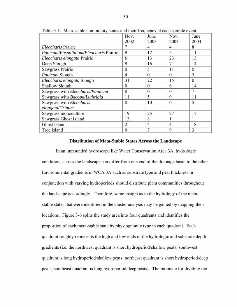
3-1 Meta-stable community states and their frequency at each sample event...............30

4-1 Hydrological variables with abbreviations..............................................................34

4-2 Neural network model statistics for each station hindcasted. PME (percent model error) = RMSE (root mean-square error) / (range of measured data). .....................38

4-3 Environmental variables used in the multivariate analyses and how they were relativized if a transformation was appropriate........................................................39

C-1 Stress in relation to dimensionality for slough NMS. A two-dimensional solution was chosen................................................................................................................81

C-2 Stress in relation to dimensionality for prairie NMS. A two-dimensional solution was chosen................................................................................................................81

C-3 Stress in relation to dimensionality for sawgrass NMS. A three-dimensional solution was chosen..................................................................................................82

C-4 Stress in relation to dimensionality for island NMS. A three-dimensional solution was chosen................................................................................................................83

ix

LIST OF FIGURES

Figure page 1-1 A community can shift to an alternate state if the perturbation is strong enough, or

conditions change steadily over time. Note that two community states can exist in the same environmental conditions. For instance, two meta-stable states can operate under the same hydrological conditions, but have different hydrologic thresholds (Scheffer 2001). ........................................................................................3

2-1 Shaded area is the location of the study area. Water Conservation Area 3A is designated as section 9 on this map. ........................................................................11

2-2 Satellite composite of the study area in Water Conservation Area 3A. Twenty plots were distributed with a stratified random design for the sampling procedures........12

2-3 An overlay of a square kilometer plot on satellite imagery. The blue dots signify reference poles aligned with belt transects within the plot. Each transect crosses at least one community boundary. ...............................................................................13

2-4 A diagram of a belt transect consisting of three traversable subtransects. Each sub transect can be sampled on four different occasions – twice on each side. .............14

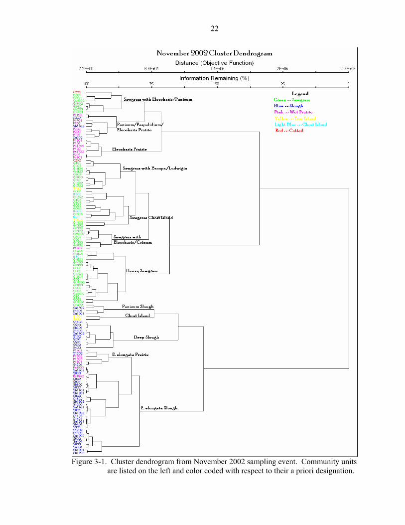
3-1 Cluster dendrogram from November 2002 sampling event. Community units are listed on the left and color coded with respect to their a priori designation. ...........22

3-2 Cluster dendrogram from June 2003 sampling event. Community units are listed on the left and color coded with respect to their a priori designation. .....................23

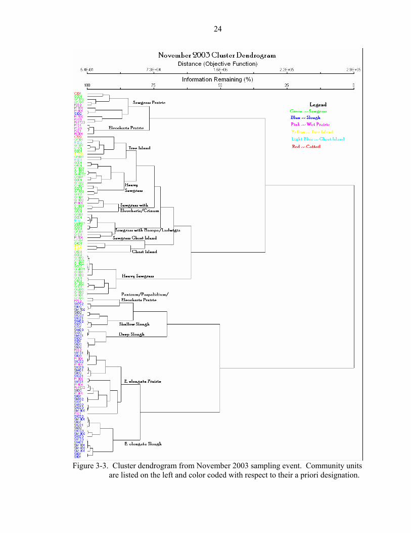
3-3 Cluster dendrogram from November 2003 sampling event. Community units are listed on the left and color coded with respect to their a priori designation. ...........24

3-4 Cluster dendrogram from June 2004 sampling event. Community units are listed on the left and color coded with respect to their a priori designation. .....................25

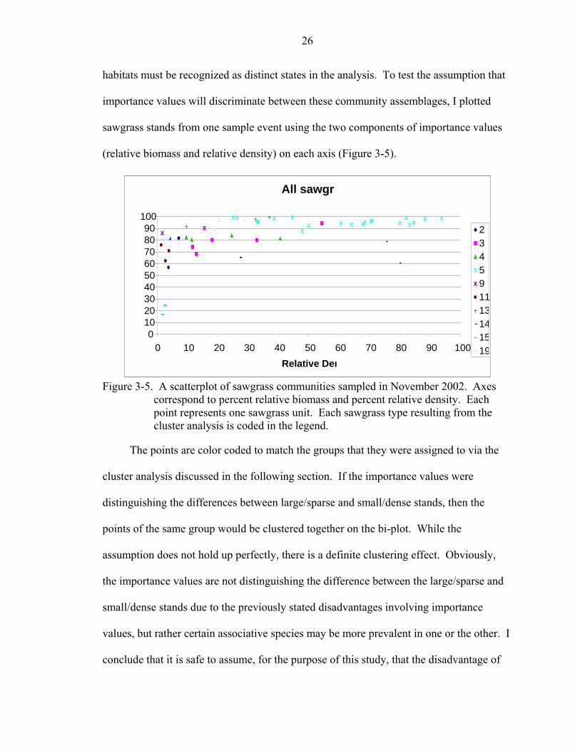
3-5 A scatterplot of sawgrass communities sampled in November 2002. Axes correspond to percent relative biomass and percent relative density. Each point represents one sawgrass unit. Each sawgrass type resulting from the cluster analysis is coded in the legend. ................................................................................26

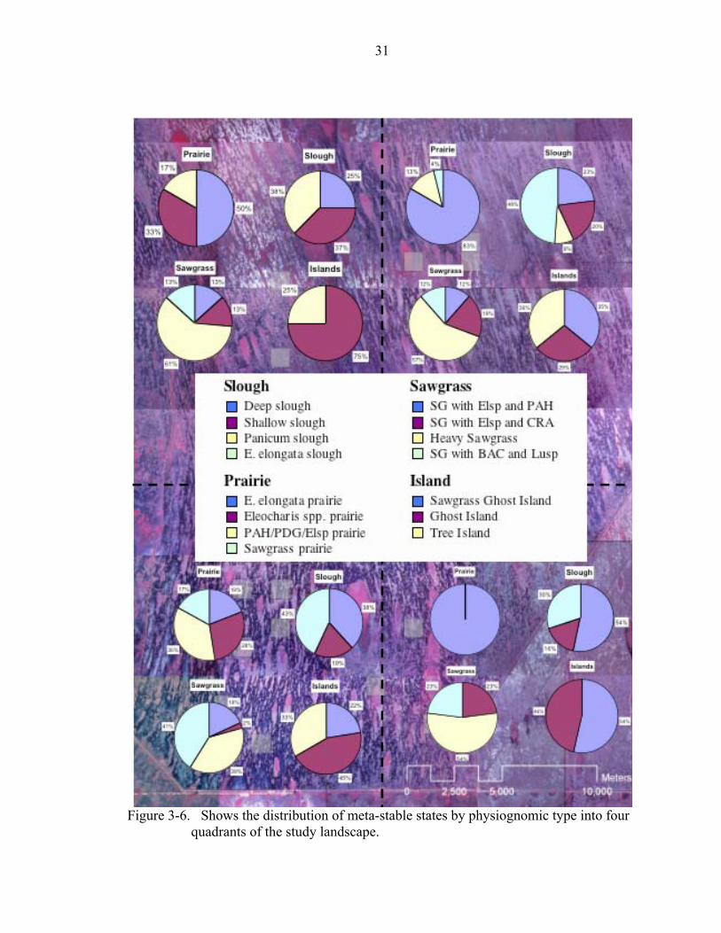
3-6 Shows the distribution of meta-stable states by physiognomic type into four quadrants of the study landscape..............................................................................31

x

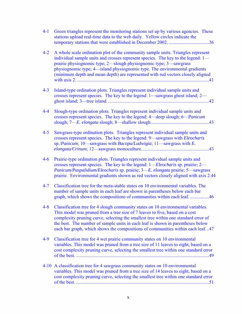
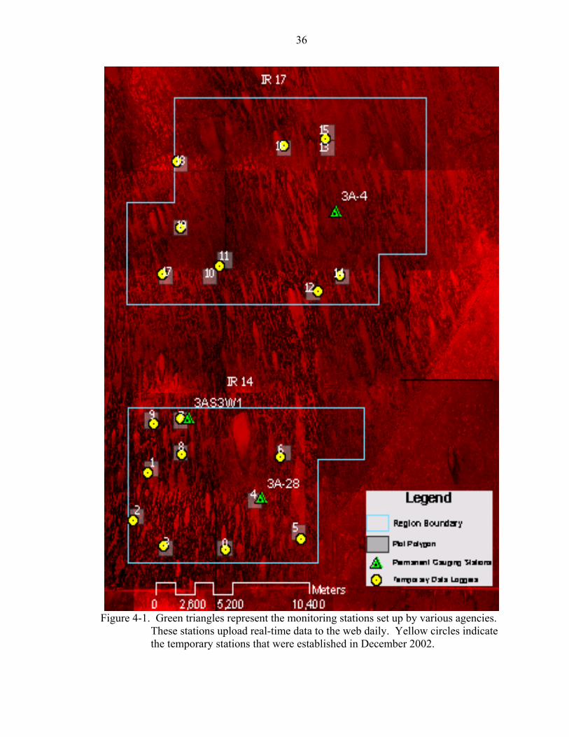
4-1 Green triangles represent the monitoring stations set up by various agencies. These stations upload real-time data to the web daily. Yellow circles indicate the temporary stations that were established in December 2002. ..................................36

4-2 A whole scale ordination plot of the community sample units. Triangles represent individual sample units and crosses represent species. The key to the legend: 1—prairie physiognomic type; 2—slough physiognomic type; 3—sawgrass physiognomic type; 4—island physiognomic type. The environmental gradients (minimum depth and mean depth) are represented with red vectors closely aligned with axis 2. ...............................................................................................................41

4-3 Island-type ordination plots. Triangles represent individual sample units and crosses represent species. The key to the legend: 1—sawgrass ghost island; 2—ghost island; 3—tree island. .....................................................................................42

4-4 Slough-type ordination plots. Triangles represent individual sample units and crosses represent species. The key to the legend: 4—deep slough; 6—Panicum slough; 7—E. elongata slough; 8—shallow slough.................................................43

4-5 Sawgrass-type ordination plots. Triangles represent individual sample units and crosses represent species. The key to the legend: 9—sawgrass with Eleocharis sp./Panicum; 10—sawgrass with Bacopa/Ludwigia; 11—sawgrass with E. elongata/Crinum; 12—sawgrass monoculture.........................................................43

4-6 Prairie-type ordination plots. Triangles represent individual sample units and crosses represent species. The key to the legend: 1—Eleocharis sp. prairie; 2—Panicum/Paspalidium/Eleocharis sp. prairie; 3—E. elongata prairie; 5—sawgrass prairie. Environmental gradients shown as red vectors closely aligned with axis 2.44

4-7 Classification tree for the meta-stable states on 10 environmental variables. The number of sample units in each leaf are shown in parentheses below each bar graph, which shows the compositions of communities within each leaf. ................46

4-8 Classification tree for 4 slough community states on 10 environmental variables. This model was pruned from a tree size of 7 leaves to five, based on a cost complexity pruning curve, selecting the smallest tree within one standard error of the best. The number of sample units in each leaf is shown in parentheses below each bar graph, which shows the compositions of communities within each leaf...47

4-9 Classification tree for 4 wet prairie community states on 10 environmental variables. This model was pruned from a tree size of 11 leaves to eight, based on a cost complexity pruning curve, selecting the smallest tree within one standard error of the best. ................................................................................................................49

4-10 A classification tree for 4 sawgrass community states on 10 environmental variables. This model was pruned from a tree size of 14 leaves to eight, based on a cost complexity pruning curve, selecting the smallest tree within one standard error of the best. ................................................................................................................51

xi

4-11 Classification tree for 3 island-type community states on 10 environmental variables. This model was pruned from a tree size of 10 leaves to eight, based on a cost complexity pruning curve, selecting the smallest tree within one standard error of the best. ................................................................................................................53

5-1 Distribution of sample units of each community state along a hydrologic variable (mean annual water depth). Communities are grouped by physiognomic type: squares=prairies, triangles=sloughs, circles=sawgrass, crosses=islands. ................57

5-2 Distribution of sample units of each community state along a peat depth gradient. Communities are grouped by physiognomic type: squares=prairies, triangles=sloughs, circles=sawgrass, crosses=islands..............................................58

5-3 A time-series graph of water stage at a monitoring station within Plot 4. Note the extreme highs and lows of the second water year compared to the first water year.59

A-1 Change in p-value from the randomization tests, averaged across species at each step in the clustering.................................................................................................67

A-2 Number of species with p ≤ 0.05 for each step of clustering. ..................................67

A-3 Change in p-value from the randomization tests, averaged across species at each step in the clustering.................................................................................................68

A-4 Number of species with p ≤ 0.05 for each step of clustering. ..................................68

A-5 Change in p-value from the randomization tests, averaged across species at each step in the clustering.................................................................................................69

A-6 Number of species with p ≤ 0.05 for each step of clustering. ..................................69

A-7 Change in p-value from the randomization tests, averaged across species at each step in the clustering.................................................................................................70

A-8 Number of species with p ≤ 0.05 for each step of clustering. ..................................70

B-1 Structural signature of the Panicum/Paspalidium/Eleocharis Prairie......................72

B-2 Structural signature of the Shallow Slough..............................................................72

B-3 Structural signature of the Ghost Island. ..................................................................73

B-4 Structural signature of the Deep Slough ..................................................................74

B-5 Structural signature of the Eleocharis elongata Slough...........................................74

B-6 Structural signature of the Eleocharis elongata Prairie. ..........................................74

B-7 Structural signature of the Sawgrass Prairie. ...........................................................75

xii

B-8 Structural signature of the Eleocharis Prairie. .........................................................75

B-9 Structural signature of the Panicum Slough.............................................................76

B-10 Structural signature of the Tree Island. ....................................................................76

B-11 Structural signature of Sawgrass with Bacopa and Ludwigia..................................77

B-12 Structural signature of the Sawgrass Ghost Island...................................................77

B-13 Structural signature of Sawgrass with E. elongata and Crinum. .............................78

B-14 Structural signature of Heavy Sawgrass...................................................................78

B-15 Structural signature of Sawgrass with Eleocharis and Panicum..............................79

C-1 A scree plot for the slough-type ordination..............................................................80

C-2 A scree plot for the prairie-type ordination. .............................................................81

C-3 A scree plot for the sawgrass-type ordination. .........................................................82

C-4 A scree plot for the island-type ordination...............................................................83

D-1 Importance rankings of predictor variables for the slough physiognomic type. ......84

D-2 Importance rankings of predictor variables for the prairie physiognomic type. ......85

D-3 Importance rankings of predictor variables for the sawgrass physiognomic type. ..85

D-4 Importance rankings of predictor variables for the island physiognomic type. .......86

xiii

Abstract of Thesis Presented to the Graduate School

of the University of Florida in Partial Fulfillment of the Requirements for the Degree of Master of Science

META-STABLE STATES OF VEGETATIVE HABITATS IN WATER CONSERVATION AREA 3A, EVERGLADES

By

Erik Powers

December 2005

Chair: Wiley Kitchens Major Department: Interdisciplinary Ecology

The Everglades consists of a constantly dynamic patchwork of vegetative

communities, confined by a matrix of levees and canals into impoundments. Water

Conservation Area (WCA) 3A is a centrally located impoundment, relatively far

downstream from the nutrient-laden waters of the Everglades Agricultural Area. The

major determinants of community structure within WCA 3A are hydrology and soil

characteristics. This study monitors plant community structure over two years, in

transects randomly stratified across the landscape, to determine what community states

manifest between marsh physiognomic types. These communities are constantly shifting

to alternate states, thus described as meta-stable states. They are identified through

unique, but related, vegetative structure, and characterized by a combination of particular

environmental conditions. The transects were sampled semiannually for species biomass

and density within ecotonal boundaries of approximately 140 communities identified a

priori, resulting in a data set of 513 community sample units. Hydrology was monitored

xiv

with surface water data loggers, and levels were hindcast 10 years prior to the beginning

of the study with neural network models. Peat depths were recorded for each of the

community units.

A hierarchical cluster analysis on the sample units for each sample event produced

distinct groups that, following an indicator species analysis, were interpreted as meta-

stable states of the four physiognomic types of communities of WCA 3A: slough, wet

prairie, sawgrass, and island-type. The fifteen meta-stable states include deep slough,

shallow slough, Panicum slough, E. elongata slough, E. elongata prairie, Eleocharis sp.

prairie, Panicum/Paspalidium/Eleocharis prairie, sawgrass prairie, sawgrass with

Eleocharis/Panicum, sawgrass with E. elongata/Crinum, heavy sawgrass, sawgrass with

Bacopa/Ludwigia, sawgrass ghost island, ghost island, and tree island. A classification

tree analysis of each physiognomic type determined that both hydrology and peat depths

were major determinants of community composition.

The meta-stable states had unique environmental characteristics when accounting

for multiple variables. However, when environmental variables are examined

individually between community states, substantial overlap of environmental thresholds

is evident. It can be concluded that the state of a community in the Everglades is

dynamic due to overlap of individual thresholds, but can potentially be predicted through

multivariate modeling. The capability to model community dynamics of Everglades

habitats is crucial to hydrological management strategies. As restoration efforts proceed,

models incorporating how communities respond to management regimes can be essential

tools in scenario analysis.

1

CHAPTER 1 INTRODUCTION

In ecology, a biological community consists of coexisting organisms that are

linked to one another through unique interactions and associations, thus forming a

complex whole. Plant communities can easily be observed in the field, as they are

relatively sessile and, given a sharp physical boundary, have well-defined ecotones.

These ecotones are usually comprised of a combination of species of the bounding

communities and some unique species as well (Kent and Coker 1992). Therefore,

communities can be identified as physiognomic types. Physiognomic types are defined

by their “species structure,” or by what species exist and their relative densities and

biomass.

The four physiognomic community types of the central Everglades, as described

by Davis (1943) and Loveless (1959), are sawgrass, wet prairie, slough, and tree islands.

These are easily recognized and usually have sharp boundaries corresponding to only a

slight change in elevation (McPherson 1973). Water covers the Everglades landscape the

vast majority of the time, leading to a widely believed theory that communities are driven

by hydrologic variables (White 1994). This study attempts to determine vegetative

community subtypes, or “meta-stable” states, within sawgrass, wet prairie, and slough.

This includes the exploration of methods that will enable scientists to document shifts

between community states and between major physiognomic community types over time.

In doing so, a physical hydrologic threshold can be associated with specific

physiognomic community types.

2

What Are Meta-stable States?

Sawgrass, slough, and wet prairie physiognomic community types exhibit

multiple assemblages and representations of plant species or multiple meta-stable steady

states. These different representations of the same community are alternate

representations and states of that community, and reflect the environmental conditions at

that point in space and time (Gunderson and Pritchard 2002). Transitions between these

“within-type” community states (tall sawgrass into short sawgrass), or between the major

physiognomic community types (e.g., sawgrass into wet prairie) are indicative of

responses to environmental change.

One example of the existence of multiple steady states is the well-documented

process of eutrophication of lakes. Two alternative states can be characterized as (a)

clear water and rooted macrophytes or (b) turbid water with planktonic algae. These

states are relatively stable, but can slip into the other due to a perturbation of a keystone

process, or the removal or addition of a keystone species (Carpenter et al. 2001). If

environmental conditions change slowly, a shift in community state can occur given the

conditions continue to change over time. Alternative states may even share some of the

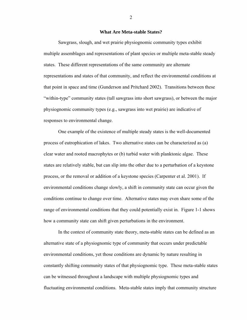
range of environmental conditions that they could potentially exist in. Figure 1-1 shows

how a community state can shift given perturbations in the environment.

In the context of community state theory, meta-stable states can be defined as an

alternative state of a physiognomic type of community that occurs under predictable

environmental conditions, yet those conditions are dynamic by nature resulting in

constantly shifting community states of that physiognomic type. These meta-stable states

can be witnessed throughout a landscape with multiple physiognomic types and

fluctuating environmental conditions. Meta-stable states imply that community structure

3

is changing in the direction that conditions are driving it, and there are no “equilibriums”

associated with them. Such is the case in the Everglades, where elevational gradients are

slight, yet hydrology fluctuates considerably on a semiannual basis. These communities

are continually stressed. The structure of the community state is a representation of

various environmental conditions presently, previously, and historically. In summary, a

meta-stable state is a representation of the trajectory of environmental conditions in the

species structure of the physiognomic type of community. The identification of meta-

stable states, as determined in this study, will be addressed in Chapter 3.

Figure 1-1. A community can shift to an alternate state if the perturbation is strong enough, or conditions change steadily over time. Note that two community states can exist in the same environmental conditions. For instance, two meta-stable states can operate under the same hydrological conditions, but have different hydrologic thresholds (Scheffer et al. 2001).

4

How Community Subtypes and Driving Forces Are Determined

Scientists define ecological resilience as the property that mediates transition

among stability domains (Holling 1973). If the stable states of a specific community can

be defined by their relative composition (species present, relative density of each species,

relative biomass of each species), then the environmental conditions that the community

state tends to persist in indicate a potential driving force. A record of historical and

present conditions of the driving force(s) at that site can lead to clues as to where

environmental thresholds lie for the current community type.

Determining community states requires identification of external (abiotic) and

internal (biological) driving forces. All biological communities have several driving

forces, some of them working in concert. However, depending on the temporal and

spatial scale of interest, some of these forces can be ignored as having negligible effect

(DeAngelis and White 1994). A study of community level processes over the course of

two years can rule out slow processes such as interglacial sea level rise, tectonic

movements, and global climate change, as well as intermediate processes such as

weathering, and soil accretion. The focus of a study such as this should be on processes

that will affect the structure of communities within the time frame of the study. In a

hydrologically driven system such as the Everglades, hydropattern is a driving force that

will have one of the strongest effects on vegetation composition and structure. For

example, recruitment of many wetland species through their respective seed and

propagule bank is dependent on meeting certain hydrologic and other criteria (van der

Valk 1990). Sawgrass (Cladium jamaicense), the archetypical plant species of the

Everglades, requires occasional drying events in order to germinate (Smith et al. 2002),

as is generally the case with emergent wetland plant species (Gerritson and Greening

5

1989). This is especially true in low nutrient regions of the Everglades where sawgrass

stands may neglect important biological functions when exposed to extremely long

hydroperiods (Weisner and Miao 2004). Emergent plants tend to allocate biomass to

shoot length and blade growth in deeper hydrologic conditions, and allocate less energy

to developing belowground rhizome biomass (Weisner and Strand 1996). In regions of

the Everglades such as southern WCA 3A that exhibit perpetually long hydroperiods and

low nutrient concentrations, sawgrass communities, though persistent, are unable to

recruit resulting in sparse, patchy distributions, rather than thick, continuous landscapes

that were present prior to drainage and impoundment (Wood and Tanner 1990). The

resulting communities are composed of emergents such as Pontederia cordata or

Sagittaria lancifolia and woody vegetation such as Cephalanthus occidentalis

interspersed with floating leaf aquatics such as Nymphaea odorata, usually associated

with deep water marshes.

Peat accretion is a slow process that is an important driving force in determining

topography and hence hydroperiod. Competing with this process is decomposition,

which may occur at a much faster rate during drought effects through oxidation or fire.

As these changes in peat depth occur, bedrock topography continues to exert a strong

influence on vegetation through its influence on the patterns of water depth and flow.

Autogenic succession may occur over long periods of time, but is probably rare (Gleason

and Stone 1994).

Other forces that could have major effects on community composition in the

Everglades and within the time frame of the study are fire, variation in nutrient supply,

freezes and wind (DeAngelis 1994). During the period of study, fire did not occur in the

6

monitoring transects, and hence was not a factor in determining community composition.

However, the history of fire for each of the transects is unknown. For the purposes of

this study, it is assumed that the transects had not been burned for a considerable time

prior to the study. Intense or repeated freezes were also not issues. A series of

hurricanes did strike Florida in the summer of 2004, however Miami-Dade County was

not in the path of any of those disturbances. The study area being investigated is far from

any upstream point source of nutrients and exotic species invasions (canals, urbanized

areas, etc.). The Everglades, historically, is an oligotrophic system, so nutrient loading

will be assumed to be constant at low levels.

Communities of the Everglades

Of the major physiognomic community types of the Everglades, I intend to focus

on three that are both naturally and anthropogenically influenced by hydrology –

sawgrass marshes, peat-based wet prairies (Eleocharis flats), and sloughs. These three

herbaceous communities all occur in southern and central WCA-3A, and often adjacent

to each other. They occur in areas with slightly different relative hydroperiods, with

sawgrass being the driest followed by wet prairie and finally slough as typically the

wettest of the physiognomic types (White 1994).

Sawgrass is the characteristic plant species of the freshwater Everglades. It is

well adapted to flooding, drought, and burning but is killed if high water levels are

prolonged (Herndon et al. 1991). Sawgrass dominates the oligotrophic fresh waters of

the Everglades due to its low nutrient requirements (Gunderson 1994). Sawgrass occurs

in strands that run longitudinally (the historical direction of water flow) in WCA 3A. It

also persists in patches of deep water in the southern extent of 3A, as well as on floating

peat mats and the outer edges of tree islands. Occasionally shrub islands appear in place

7

of burned or drowned tree islands and sawgrass strands. Cephalanthus occidentalis and

Pontederia cordata are common associates of sawgrass in these transitional

physiognomic types. Islands and their transitional states will also be examined in this

study.

Wet prairies can be classified into two groups—peat-based and marl-based. Marl-

based wet prairies are confined to the marl wetlands situated in the Everglades National

Park, and were not included in this study. Peat-based prairies can further be divided into

three types—Eleocharis, Rhynchospora, and Panicum flats. Of these types, only

Eleocharis, or spikerush, flats, and Panicum, or maidencane flats, are present in the study

area. Rhynchospora prairies are relatively rare after the impoundment of the Everglades.

Wet prairies are typically more diverse than sawgrass or slough communities and occur

often as transitional communities in deeper areas where slough communities are

prevalent (Gunderson 1994) or between slough and sawgrass community as a transitional

community.

Slough communities consist of associations of floating-leafed aquatic plants and

are generally the wettest of the communities in WCA-3A. Submerged aquatics are also

associated with sloughs and provide structure for periphyton, the main source of primary

production in the freshwater Everglades (Gunderson 1994).

Each of these communities has been observed in different forms and structure, yet

they are documented in the general body of scientific literature as single communities.

This project presents evidence that these alternative community states are characteristic

of the environmental conditions at that site. More importantly, transitions between

alternative states of one physiognomic type may occur more readily than a shift between

8

major physiognomic types. In other words, the resilience of a major physiognomic

community type is greater than the resilience of one of its alternate states. This is tested

through the identification of the hydrologic ranges of each meta-stable state. If there is a

substantial overlap of hydrology between meta-stable states of communities, then it can

be concluded that a shift to an alternate community state while maintaining its basic

physiognomic community type is a possible response to extended exposure to threshold

conditions (see Figure 1-1).

Project Objectives

With this research, I intend to describe the multiple meta-stable states of

physiognomic marsh types of Water Conservation Area 3A in terms of community

structure and their respective environmental tolerances. First, through tabulating relative

densities and relative biomass of species present on established transects during wet and

dry seasons, the current state of a community at any given point in time during the study

was identified. Vegetative community monitoring efforts will continue for two years,

sampling at a rate of twice a year for a total of four sampling events. Hydrologic ranges

for the various meta-stable states of sawgrass, slough, and wet prairie are identified and

each community state is characterized by its environmental variables using classification

trees. Inferences, based on the range of conditions that a state may tolerate, can be made

on the dynamics and resiliency of various vegetative meta-stable states.

Although the study monitors communities over time, tracking the change of

specific sites over time was not included in the scope of this project. The temporal scope

of this study is limited to observing communities under different seasons and water years

to capture the various community states that might manifest under those conditions.

9

CHAPTER 2 DETERMINING COMMUNITY STRUCTURE

Everglades communities were originally identified by the dominant species

associated with a congregation of smaller or less prevalent species. Loveless first

documented vegetative assemblages in the Everglades (Loveless 1959). Several types of

sawgrass, wet prairie, and slough communities were identified through the abundance

and densities of dominant and associative species. His descriptions of vegetative

communities serve as an introduction and as the basis of comparison for the communities

revealed in the following analyses. The following community types were identified by

Loveless:

Cladium – Sagittaria – Panicum hemitomon: This sawgrass community can occur

in sparse, dense, or monotypic stands of sawgrass. It is associated with duck potato and

maidencane, as well as a suite of other species depending on the density of sawgrass.

Species composition tends to vary between the dry and wet seasons.

Cladium – Myrica – Ilex: A drier community of sawgrass, this congregation of

species includes woody thickets of buttonbush, wax myrtle, and dahoon holly.

Cladium – Panicum hemitomon: Similar to the duck potato/maidencane sawgrass

community, but occupies drier sites. Densities range from sparse to moderately thick.

Rhynchospora Flats: This community was more prevalent during predrainage

conditions. The wettest of the Loveless communities except for sloughs, this assemblage

includes beakrush as the dominant species and spikerush as the common associate. These

communities are typically found adjacent to sawgrass and shrub island communities.

10

Panicum hemitomon Flats: Maidencane is the dominant member of this

community and usually occupies drier sites. This community is resilient to fire and can

withstand long periods of flooding while maintaining its basic species configuration.

Associative species usually include spikerush and spider lilies.

Eleocharis Flats: Easily recognizable as monotypic stands of spikerush. This

community is usually found along the southern and western reaches of Water

Conservation Area 3A.

Sloughs: The wettest of the communities, sloughs are usually filled with water year

round. Species associated with sloughs are floating water lily, bladderwort, and

spatterdock. Sloughs comprise the drainage vectors of the Everglades, running generally

longitudinally along the landscape in a north-south direction.

The communities described by Loveless, while useful from a naturalist’s

perspective, are outdated with respect to the decades of impoundment effects on

Everglades ecology and irrelevant to studying short-term succession. Communities of the

Everglades are dynamic on two time scales: seasonal and long term (multiannual).

Subtropical south Florida has two distinct hydrologic seasons – a wet season during the

summer and fall months, and a dry season during the winter and spring months. Changes

in hydrology imposed by both seasonal fluctuations and water regimes managed by state

agencies will have subtle if not profound effects on community composition. If

restoration agents mean to influence the ecology area from the bottom-up, that is “get the

water right”, then the scientific lens must focus on the immediate responses of plant

communities that provide wildlife habitat to variations in hydrology.

11

Description of Study Site

The study was conducted in the southern half of Water Conservation Area 3A

located in Dade and Broward counties (see Figure 2-1). Bounded by Tamiami Trail to

the south, Holiday Trail (a heavily trafficked airboat trail) to the north, Big Cypress

National Preserve to the west, and Water Conservation Area 3B to the east, the study site

is made up of a matrix of freshwater habitats ranging from short hydroperiod bay and

willow tree islands to deep water sloughs. Strands of sawgrass run longitudinally,

divided by wet prairie and slough. This area was chosen because of the smattering of

distinct communities, abundance of ecotones, and noticeable elevational gradients on a

landscape scale as well as community scale. The total area of the study site is 62,000

hectares.

Figure 2-1. Shaded area is the location of the study area. Water Conservation Area 3A is designated as section 9 on this map.

12

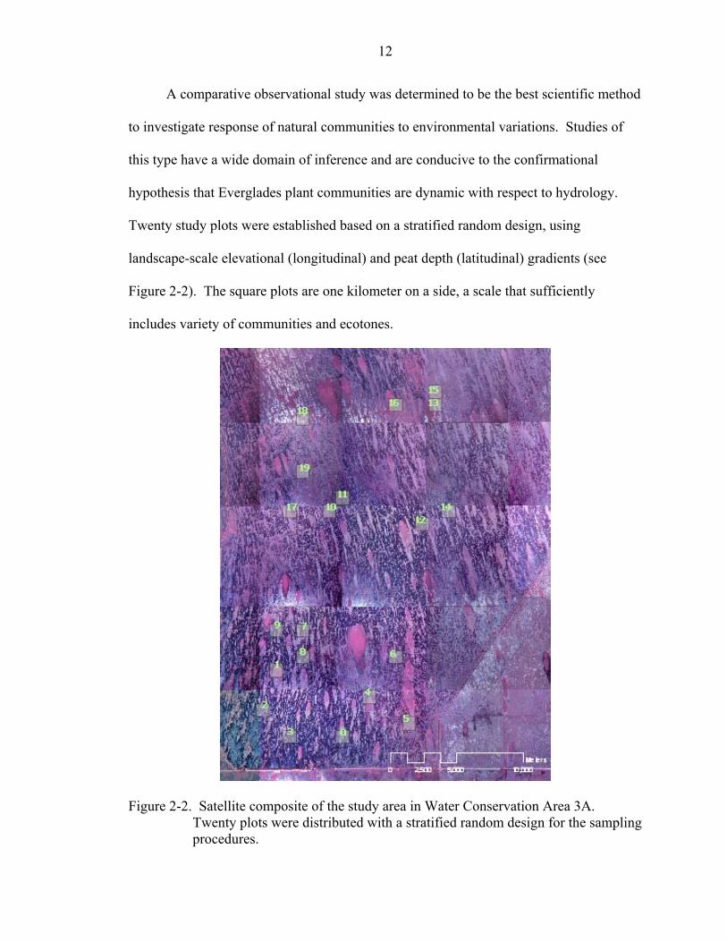
A comparative observational study was determined to be the best scientific method

to investigate response of natural communities to environmental variations. Studies of

this type have a wide domain of inference and are conducive to the confirmational

hypothesis that Everglades plant communities are dynamic with respect to hydrology.

Twenty study plots were established based on a stratified random design, using

landscape-scale elevational (longitudinal) and peat depth (latitudinal) gradients (see

Figure 2-2). The square plots are one kilometer on a side, a scale that sufficiently

includes variety of communities and ecotones.

Figure 2-2. Satellite composite of the study area in Water Conservation Area 3A. Twenty plots were distributed with a stratified random design for the sampling procedures.

13

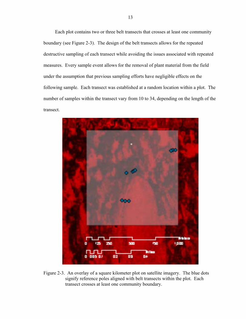
Each plot contains two or three belt transects that crosses at least one community

boundary (see Figure 2-3). The design of the belt transects allows for the repeated

destructive sampling of each transect while avoiding the issues associated with repeated

measures. Every sample event allows for the removal of plant material from the field

under the assumption that previous sampling efforts have negligible effects on the

following sample. Each transect was established at a random location within a plot. The

number of samples within the transect vary from 10 to 34, depending on the length of the

transect.

Figure 2-3. An overlay of a square kilometer plot on satellite imagery. The blue dots signify reference poles aligned with belt transects within the plot. Each transect crosses at least one community boundary.

14

Methods and Materials

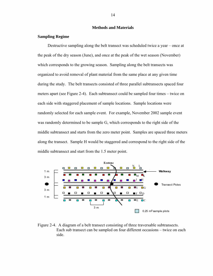
Sampling Regime

Destructive sampling along the belt transect was scheduled twice a year – once at

the peak of the dry season (June), and once at the peak of the wet season (November)

which corresponds to the growing season. Sampling along the belt transects was

organized to avoid removal of plant material from the same place at any given time

during the study. The belt transects consisted of three parallel subtransects spaced four

meters apart (see Figure 2-4). Each subtransect could be sampled four times – twice on

each side with staggered placement of sample locations. Sample locations were

randomly selected for each sample event. For example, November 2002 sample event

was randomly determined to be sample G, which corresponds to the right side of the

middle subtransect and starts from the zero meter point. Samples are spaced three meters

along the transect. Sample H would be staggered and correspond to the right side of the

middle subtransect and start from the 1.5 meter point.

N L

M KJ H

I G

F D

E C

Figure 2-4. A diagram of a belt transect consisting of three traversable subtransects. Each sub transect can be sampled on four different occasions – twice on each side.

15

Sampling Methodology

The area of each sample is determined by a .25 square-meter circular hoop with

its center around a dowel placed at the sample point offset from the subtransect by a

meter. The dowel marks the sample point and allows for a reference when the hoop has a

tendency to float or deviate from its original placement. Floating vegetation is collected

from the sample first. After the floating vegetation is removed any material that may

subsequently drift into the sample area is disregarded. The rooted vegetation is then cut

at the soil surface and collected. All vegetation is collected in burlap sacks to allow some

air exchange for the evaporation of excess moisture. The vegetation remained more

resistant to disintegration and mold when stored in burlap rather than being stored in

plastic.

During the sample harvest, rotten material, determined by its structural integrity,

was discarded. For example, if the material when given a gentle shake did not maintain

any rigidity, than the material was deemed to be rotten and associated with the peat

substrate. Rotten vegetation was difficult to identify and proved almost impossible to

quantify. This structural integrity test provided consistent and comprehensive criteria for

determining viable plant material.

Samplers remained within the one meter wide subtransect path to avoid walking

on sample locations. Water depths were measured at each sample point and at the

transect start and end poles for reference points to be tied back in to the monitoring wells

for continuous hydrologic data for each sample point. Samples for the transect were

labeled and loaded into an airboat for transport back to a refrigerated storage unit. A total

of 1190 samples were collected from the study area per sample event.

16

Processing Methodology

Each sample was sorted by species and the numbers of individuals were tabulated

for each species. Counts for Eleocharis, Pontederia, Nymphaea, Bacopa, Crinum, and

woody vegetation were determined by the number of emergent stems. Cladium and

Typha counts were determined by the number of emergent culms. Utricularia and Chara

counts were impossible to determine in the laboratory and were tabulated as either

present or absent. Species for each sample were separated into paper bags, labeled, and

dried for at least two weeks in walk-in ovens set at 140°F. Dried plant material avoids

the inclusion of water weights that can vary considerably between species. After the

samples were dried, the dry biomass for each species was measured on digital scales to

the nearest hundredth of a gram. The dried plant material was then discarded into

compost. Biomass and count data were transcribed into an Excel spreadsheet in

accordance with appropriate quality control measures. See Table 2-1 for a complete

species list.

Data Preparation and Relativization

Community units are heretofore defined as the conglomeration of the samples

within one of the physiognomic community units represented in a transect. Each

community unit is designated with a plot number, transect number, a priori

physiognomic type, and sample event. A priori physiognomic types include cattail (C),

sawgrass (G), ghost island (I), prairie (P), slough (S), and tree island (T). These habitats

are important to aquatic macrofauna and are used differently by various suites of species

(e.g., Loftus and Kushlan 1987, Gunderson and Loftus 1993, Jordan et al. 1994, 1996).

The sample event is designated by where within the belt transect the community was

sampled for that sample collection. Sample events include: G – November 2002, E –

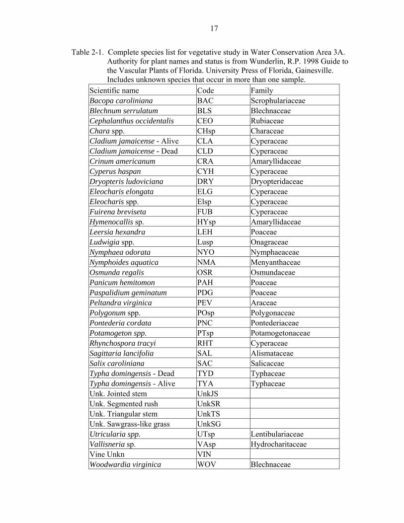
17

Table 2-1. Complete species list for vegetative study in Water Conservation Area 3A. Authority for plant names and status is from Wunderlin, R.P. 1998 Guide to the Vascular Plants of Florida. University Press of Florida, Gainesville. Includes unknown species that occur in more than one sample.

Scientific name Code Family Bacopa caroliniana BAC Scrophulariaceae Blechnum serrulatum BLS Blechnaceae Cephalanthus occidentalis CEO Rubiaceae Chara spp. CHsp Characeae Cladium jamaicense - Alive CLA Cyperaceae Cladium jamaicense - Dead CLD Cyperaceae Crinum americanum CRA Amaryllidaceae Cyperus haspan CYH Cyperaceae Dryopteris ludoviciana DRY Dryopteridaceae Eleocharis elongata ELG Cyperaceae Eleocharis spp. Elsp Cyperaceae Fuirena breviseta FUB Cyperaceae Hymenocallis sp. HYsp Amaryllidaceae Leersia hexandra LEH Poaceae Ludwigia spp. Lusp Onagraceae Nymphaea odorata NYO Nymphaeaceae Nymphoides aquatica NMA Menyanthaceae Osmunda regalis OSR Osmundaceae Panicum hemitomon PAH Poaceae Paspalidium geminatum PDG Poaceae Peltandra virginica PEV Araceae Polygonum spp. POsp Polygonaceae Pontederia cordata PNC Pontederiaceae Potamogeton spp. PTsp Potamogetonaceae Rhynchospora tracyi RHT Cyperaceae Sagittaria lancifolia SAL Alismataceae Salix caroliniana SAC Salicaceae Typha domingensis - Dead TYD Typhaceae Typha domingensis - Alive TYA Typhaceae Unk. Jointed stem UnkJS Unk. Segmented rush UnkSR Unk. Triangular stem UnkTS Unk. Sawgrass-like grass UnkSG Utricularia spp. UTsp Lentibulariaceae Vallisneria sp. VAsp Hydrocharitaceae Vine Unkn VIN Woodwardia virginica WOV Blechnaceae

18

June 2003, D – November 2003, and J – June 2004. For example, P18E2 refers to the

prairie community in plot 18, transect 2, sampled on event E (June 2003).

Prior to relativizing the data, I deleted samples that were missing count or

biomass data. This amounted to approximately 1% of the total sample. I also removed

samples that occurred adjacent to the ecotone. Locations of ecotones were determined in

the field by noting the samples between which dominant species appear and disappear,

indicating a different physiognomic type. The definitions of the a priori communities

were used to determine physiognomic types. Ecotones in the conservation area are

typically sharp and distinguishable allowing for minimal observer error in designating

ecotone location. This was done to remove samples that may be considered to be

transitional or not a typical representation of that community unit. Approximately 85%

of the samples remained in the analysis and are assumed to be representative of the

community units sampled.

The community data was converted into relative proportions for each community

unit sampled. Counts for each species in every sampled community were expressed as

the relative density of that species. For example, the relative density of Eleocharis in

community unit P18E2 equals the total count of Eleocharis stems in P18E2 divided by

the total count of all species in community unit P18E2. Relative biomass was calculated

in similar fashion equaling the proportion of the total biomass of a species in that

community unit to the total biomass of all species in that unit.

Averaging the relative density and relative biomass results in an importance value

for each species in each community unit. The advantage of using importance values in

ecological community analysis is that they are equally influenced by large biomasses and

19

large stem densities, so that species that differ in size and density can be compared within

the same sample unit. The disadvantage of importance values is that a species that has

large biomass values and sparse densities can have the same importance value as a

species with small biomass values and high densities (McCune and Grace 2002). Later I

will discuss how I tested the assumption that importance values can distinguish different

community stands, regardless of the vulnerability associated with importance values.

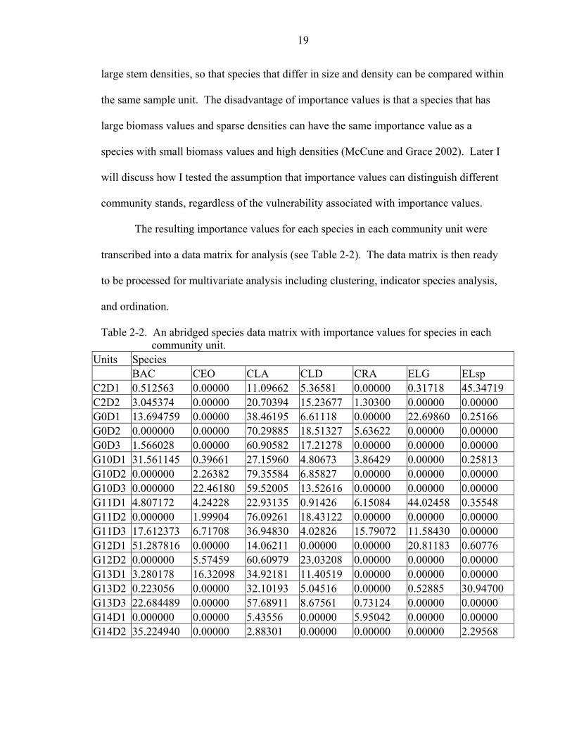
The resulting importance values for each species in each community unit were

transcribed into a data matrix for analysis (see Table 2-2). The data matrix is then ready

to be processed for multivariate analysis including clustering, indicator species analysis,

and ordination.

Table 2-2. An abridged species data matrix with importance values for species in each community unit.

Units Species BAC CEO CLA CLD CRA ELG ELsp C2D1 0.512563 0.00000 11.09662 5.36581 0.00000 0.31718 45.34719 C2D2 3.045374 0.00000 20.70394 15.23677 1.30300 0.00000 0.00000 G0D1 13.694759 0.00000 38.46195 6.61118 0.00000 22.69860 0.25166 G0D2 0.000000 0.00000 70.29885 18.51327 5.63622 0.00000 0.00000 G0D3 1.566028 0.00000 60.90582 17.21278 0.00000 0.00000 0.00000 G10D1 31.561145 0.39661 27.15960 4.80673 3.86429 0.00000 0.25813 G10D2 0.000000 2.26382 79.35584 6.85827 0.00000 0.00000 0.00000 G10D3 0.000000 22.46180 59.52005 13.52616 0.00000 0.00000 0.00000 G11D1 4.807172 4.24228 22.93135 0.91426 6.15084 44.02458 0.35548 G11D2 0.000000 1.99904 76.09261 18.43122 0.00000 0.00000 0.00000 G11D3 17.612373 6.71708 36.94830 4.02826 15.79072 11.58430 0.00000 G12D1 51.287816 0.00000 14.06211 0.00000 0.00000 20.81183 0.60776 G12D2 0.000000 5.57459 60.60979 23.03208 0.00000 0.00000 0.00000 G13D1 3.280178 16.32098 34.92181 11.40519 0.00000 0.00000 0.00000 G13D2 0.223056 0.00000 32.10193 5.04516 0.00000 0.52885 30.94700 G13D3 22.684489 0.00000 57.68911 8.67561 0.73124 0.00000 0.00000 G14D1 0.000000 0.00000 5.43556 0.00000 5.95042 0.00000 0.00000 G14D2 35.224940 0.00000 2.88301 0.00000 0.00000 0.00000 2.29568

20

CHAPTER 3 CLASSIFICATION OF META-STABLE STATES

In order to determine how the vegetative habitats of the Everglades change in

response to continuously varying environmental conditions, identification of the meta-

stable states in which they are observed is required. Informal observation of plant

communities in Water Conservation Area 3A yields four physiognomic community

types: sawgrass, wet prairie, slough, and shrub/tree island. Ghost islands are also a

distinguishable community as old sawgrass ridges or islands that have experienced a

disturbance such as extreme flooding or fire. Ghost islands generally have some sparse

sawgrass, pickerelweed and buttonbush associated with them. Cattail (Typha spp.)

communities can also be observed, however there were only two community units

sampled that had cattail as a major component.

Subtle differences in the composition within these physiognomic types require the

statistical analysis of hierarchical classification. Classification through hierarchical

cluster analyses is necessary to identify these meta-stable community states and

recognize the subtle differences in community structure between these states. Meta-

stable states will be identified as discernable subunits of physiognomic types. In the

Everglades, these meta-stable states will be represented through the range of

environmental conditions that physiognomic types in WCA 3A exhibit. After the cluster

analyses, environmental conditions at those sites are investigated to produce profiles of

environmental conditions and thresholds.

21

Hierarchical Agglomerative Cluster Analysis

I used the species matrices referenced in Chapter 2 to apply a hierarchical

agglomerative cluster analysis. Each matrix contains importance values for every species

in each community unit for a particular sampling event. In all, there were four sample

events yielding four matrices with the same community units in each matrix.

Agglomerative clustering methods build groups hierarchically from the bottom up,

forming groups by fusing similar subgroups together (McCune and Grace 2002). The

optimal number of groups is calculated through an indicator species analysis. Cluster

analyses first calculate a matrix of distances between each pair of entities. Groups that

meet the minimum distance criteria are merged and their attributes combined. The

merging process continues until there is only one group. The result is a dendrogram

complete with a distance measure (from the distance matrix). The distance measure is a

function of the information lost at each clustering step (Wishart 1969).

The cluster analysis was performed on the PC-Ord software using a Euclidian

(Pythagorean) distance measure. Ward’s linkage method was chosen for its

combinatorial compatibility. Ward’s method also conserves the properties of the original

space as group attributes merge, keeping the Euclidian distances consistent throughout

the analysis (Wishart 1969). Community units were color coded by a priori classification

of physiognomic community types based on observation in the field. See Figures 3-1, 3-

2, 3-3, and 3-4 for the resulting dendrograms for each sampling event.

Testing Importance Value Assumptions

As mentioned previously, importance values have one major disadvantage in that a

large, sparse stand has the same value as a small, dense stand. Because the purpose of

this study is to discriminate between vegetative community states by their structure, those

22

Figure 3-1. Cluster dendrogram from November 2002 sampling event. Community units

are listed on the left and color coded with respect to their a priori designation.

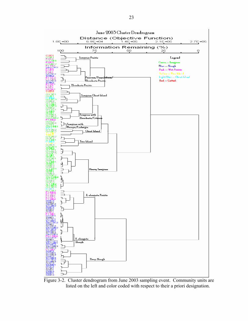
23

Figure 3-2. Cluster dendrogram from June 2003 sampling event. Community units are

listed on the left and color coded with respect to their a priori designation.

24

Figure 3-3. Cluster dendrogram from November 2003 sampling event. Community units

are listed on the left and color coded with respect to their a priori designation.

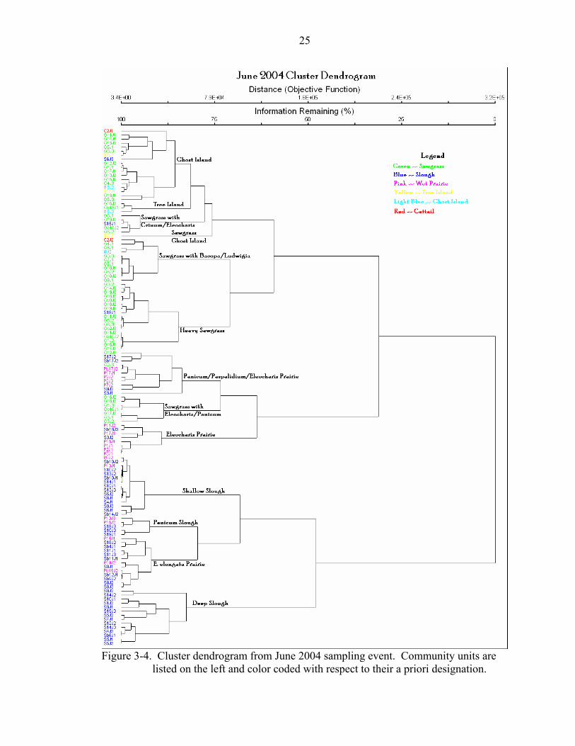
25

Figure 3-4. Cluster dendrogram from June 2004 sampling event. Community units are

listed on the left and color coded with respect to their a priori designation.

26

habitats must be recognized as distinct states in the analysis. To test the assumption that

importance values will discriminate between these community assemblages, I plotted

sawgrass stands from one sample event using the two components of importance values

(relative biomass and relative density) on each axis (Figure 3-5).

All sawgr

0102030405060708090

100

0 10 20 30 40 50 60 70 80 90 100Relative Den

234591113141519

Figure 3-5. A scatterplot of sawgrass communities sampled in November 2002. Axes

correspond to percent relative biomass and percent relative density. Each point represents one sawgrass unit. Each sawgrass type resulting from the cluster analysis is coded in the legend.

The points are color coded to match the groups that they were assigned to via the

cluster analysis discussed in the following section. If the importance values were

distinguishing the differences between large/sparse and small/dense stands, then the

points of the same group would be clustered together on the bi-plot. While the

assumption does not hold up perfectly, there is a definite clustering effect. Obviously,

the importance values are not distinguishing the difference between the large/sparse and

small/dense stands due to the previously stated disadvantages involving importance

values, but rather certain associative species may be more prevalent in one or the other. I

conclude that it is safe to assume, for the purpose of this study, that the disadvantage of

27

using importance values in this study is not relevant due to mitigating variables such as

species associates.

Indicator Species Analysis

Following the generation of cluster dendrograms, an indicator species analysis

provides a subjective determination of the optimal number of groups based on how well

any of the species acts as a significant indicator of a group. Dufrêne and Legendre’s

(1997) method of calculating species indicator values combines information on the

concentration of species importance values and the faithfulness, or endemism, of a

species to a particular group. Indicator values are tested for statistical significance using

1000 Monte Carlo randomizations.

Each sample event was subjected to an indicator species analysis on the PC-Ord

software 29 times, testing statistical significance of every species from 30 groups to 2

groups. The program provided a table for each species and a p-value, or the proportion of

randomized trials with an indicator value equal to or exceeding the observed indicator

value. Average p-values for each run and number of significant species (p<0.05) were

plotted in a spreadsheet (see Appendix A). Both plots were used to determine the optimal

number of groups to prune the cluster dendrogram. Low average p-values across the

suite of species, and high numbers of significant species determined the number of

groups. Thirteen groups of community units developed from the November 2002, June

2003, and June 2004 sampling data. Fourteen groups of community units developed

from the November 2003 sampling data.

The indicator species analysis also produces a table of indicator values, or the

percent of perfect indication based on combining the values for relative magnitude and

28

relative frequency of importance values, for each species. These tables were translated

into graphical signatures for each community state (See Appendix B). The resulting

structural signature was an important guide to describing the groups, or meta-stable

community states. Species with high indicator values (>15%) were significant species of

that community. The resulting community states and their descriptions are shown on the

cluster dendrograms in Figures 3-1, 3-2, 3-3, and 3-4.

Matching Similar Community Descriptions Between Sampling Events

The groups resulting from the cluster analyses were translated into meta-stable state

entities, as defined in Chapter 1. In this study, the meta-stable states are groups of similar

clusters that were consolidated across sample events and in some cases within events. As

a result, the community states identified represent the range of states that occurred

throughout the landscape through different seasonal and annual environmental

conditions. Some of these states were persistent through the study period, and some

occur infrequently. The following is a description of the methods used to group clusters

together across and within sample events, and define them as meta-stable community

states.

A general description of each group arising from the cluster and indicator species

analyses was constructed for each sampling event. In order to facilitate matching

community states between events, a multi-response permutation procedure (MRPP) was

utilized. MRPP is a nonparametric procedure for testing the hypothesis of no difference

between entities (Biondini et al. 1985). Each community unit was tested for

heterogeneity over time. In other words, if a community unit was similar over the four

sampling events, or minimal change had occurred over the course of monitoring, then

29

that unit would receive a low p-value. Units that exhibit little change can be associated

with the same meta-stable community state described in the indicator species analysis.

The MRPP procedure helped with establishing only four of the community state

descriptions and was insufficient in finding similar states between sample events.

Another approach, used as a complementary analysis to the MRPP, was an agglomerative

clustering process applied to all of the groups resulting from the cluster analyses of the

four sample events. Similar community states should cluster together. Most of the

resulting clusters of groups included only one group from each sample event,

corroborating that those states are unique within sample events and indicating that they

are common throughout the study period. These were designated as the community

states of the major physiognomic types. Two clusters included groups from the same

sample event that were similar: the heavy sawgrass group consists of two combined

clusters in June 2003 and November 2003, and the E. elongata slough consists of two

combined clusters in November 2002. Other community groups may have been

represented only two or three times over the four sampling events. This method of

defining groups over multiple sampling events provided an objective approach to

comparing group structural signatures, and was a potential check on the first set of cluster

analyses. If the differences of groups within sample events are less than the differences

among groups then those clusters can be essentially combined. See Table 3-1 for a list of

meta-stable community states and the frequency of community units in each event.

Discussion of these results continues in chapter 5.

30

Table 3-1. Meta-stable community states and their frequency at each sample event. Nov.

2002 June 2003

Nov. 2003

June 2004

Eleocharis Prairie 7 4 4 8 Panicum/Paspalidium/Eleocharis Prairie 9 12 5 11 Eleocharis elongata Prairie 6 13 23 13 Deep Slough 9 16 7 14 Sawgrass Prairie 0 5 11 0 Panicum Slough 4 0 0 5 Eleocharis elongata Slough 31 22 15 0 Shallow Slough 0 0 6 14 Sawgrass with Eleocharis/Panicum 8 0 0 7 Sawgrass with Bacopa/Ludwigia 11 5 9 11 Sawgrass with Eleocharis elongata/Crinum

8 10 6 5

Sawgrass monoculture 19 25 27 17 Sawgrass Ghost Island 13 8 1 1 Ghost Island 2 4 4 18 Tree Island 0 7 9 3

Distribution of Meta-Stable States Across the Landscape

In an impounded hydroscape like Water Conservation Area 3A, hydrologic

conditions across the landscape can differ from one end of the drainage basin to the other.

Environmental gradients in WCA 3A such as substrate type and peat thickness in

conjunction with varying hydroperiods should distribute plant communities throughout

the landscape accordingly. Therefore, some insight as to the hydrology of the meta-

stable states that were identified in the cluster analysis may be gained by mapping their

locations. Figure 3-6 splits the study area into four quadrants and identifies the

proportion of each meta-stable state by physiognomic type in each quadrant. Each

quadrant roughly represents the high and low ends of the hydrologic and substrate depth

gradients (i.e. the northwest quadrant is short hydroperiod/shallow peats; southwest

quadrant is long hydroperiod/shallow peats; northeast quadrant is short hydroperiod/deep

peats; southeast quadrant is long hydroperiod/deep peats). The rationale for dividing the

31

Figure 3-6. Shows the distribution of meta-stable states by physiognomic type into four

quadrants of the study landscape.

32

landscape into square quadrants is simply for convenience since the extent of

impoundment effects on the hydroscape have not been determined and a detailed survey

of peat depths in the conservation have yet to be produced.

Examination of the distribution of meta-stable states shows several insightful

trends. Sawgrass communities showed little difference in change across the landscape.

There was a slight increase in the share of Panicum and Bacopa associated sawgrass

communities towards the western extents of the impoundment area. Among prairie

communities the Eleocharis cellulosa state was confined strictly to the west whereas the

Eleocharis elongata states increased dramatically further east, which resembles the peat

depth and substrate type gradients. This suggests that the state that a wet prairie might

exhibit has a lot to do with substrate properties. Not surprisingly, deep sloughs

dominated by water lilies were more prevalent in the longer hydroperiod south. Tree

island types of islands dominated by woody vegetation and shade tolerant herbaceous

species were virtually nonexistent in the southeast.

33

CHAPTER 4 MULTIVARIATE ANALYSIS AND RESULTS

Hydrology

Selecting Hydrologic Variables

The multivariate approach to statistical analysis of data allows the researcher to test

simultaneously for significance among variables. There are many factors that may have a

hand in the makeup of community assemblages, but hydrology is the main environmental

force driving Everglades community structure. In order to include hydrology in the

statistical analysis of data, it was necessary to first determine which metrics can best

represent the hydrology of the Everglades. A set of hydrological variables was selected a

priori and calculated for each sample unit. Table 4-1 lists the hydrologic variables

selected along with the ecological rationale underlying their use.

Hydrology can be described to reflect one or several different aspects of flooding:

depth, duration, time, and the magnitude of extreme events of flooding and drought

(Richter et al. 1997). The fraction of the year that a given site is inundated was chosen

due to the prominence in the literature, especially regarding the Everglades and ease of

calculation (Toner and Keddy 1997). The mean depth of flooding, whether it be above or

below the ground surface was selected to represent the depth of water that species must

adapt to. Range of depths defines the amount of water level fluctuation that occurs

during a year. Flooding and drought event legacies are a function of the length of time

used for hydrological records to calculate hydrology. Therefore, inundation times were

calculated using one, three, five, and ten-year time records. If there is a consistent period

34

Table 4-1. Hydrological variables with abbreviations. Abbreviation Variable Units Ecological implications (T)yr.inun* Number of days per

year during which flooding occurred (inundated)

days Reproduction of some species. Exposure of soils to oxidation processes.

MeanDepth Mean depth of flooding over a ten year period

feet Establishment of aquatic vs. emergent species.

max Average 7-day maximum water depths over 10 years

feet Anaerobic stress in plants. Spatial extent of extreme conditions.

datemax Average Julien date of maximum water levels

day of year

Coordination of hydrologic factors with temperature and photic factors.

highdurat Duration of high water levels

days Anaerobic stress in emergent wetland species.

min Average 7-day minimum water depths over 10 years

feet Indication of potential oxidation of soils. Reproduction opportunities.

datemin Average Julien date of minimum water levels

day of year

Coordination of hydrologic factors with temperature and photic factors.

lowdurat Duration of low water levels

days Opportunities for emergents to develop and compete against floating leaf aquatics. Exposure of soils to oxidation processes.

variation Average annual range of depth

feet Amount of variation in the environment that must be tolerated.

* (T) denotes the length of record used to calculate the metric. Periods of time used to measure inundation time are 1, 3, 5, and 10 years. All of the other metrics are calculated using a 10-year time span.

of time that hydrology affects into the future then it would be revealed in the

classification tree analysis. Duration of typical high and low water level events were

calculated using the algorithms in the IHA (Indicators of Hydrologic Analysis) software

(Richter et al 1996). Finally, extremes during the average year were calculated as seven-

day highs and lows. Timing of these extremes was considered. These metrics were

chosen due to literature citing the importance of extreme, stochastic events in the

35

Everglades that occur periodically and play an important role in community dynamics by

offering opportunities for species recruitment, movement, and nutrient availability that

otherwise are unavailable (Kitchens et al. 2002).

Calculating Hydrologic Variables

The hydrologic data collected was processed extensively in order to be applied to

the multivariate analysis as the metrics that relevantly described the hydrology of the

sites for the community sample units. The monitoring wells were set up shortly

following the first sample event. Water data had to be extrapolated up to ten years prior

to November 2002. The well data also needed to be applied to the various sample units

that it was monitoring. The community units required classification of their elevations in

order to get depths that were relative to the well monitoring that plot. The following is a

discussion of the methodology used to calculate those hydrologic profiles.

Hindcasting using neural networks

To calculate the hydrologic variables mentioned previously, precise water data

dating back ten years was needed for the study plots. Prior to the study there were three

permanent gauging stations, established by various state and federal agencies, within the

study area (See Figure 4-1). Two of these three stations, 3-64 and 3-65, had been

established and collecting data longer than ten years prior to 2002. The agency

monitoring stations and their data was not sufficient for producing hydropatterns at each

of the 20 study plots. A network of monitoring stations needed to be established that

could provide accurate hydrologic data at the community scale.

Although the vast majority of WCA 3A is flooded most of the time, a flat pool of

water cannot be assumed over such an expansive landscape. Since the plot size was a

36

Figure 4-1. Green triangles represent the monitoring stations set up by various agencies.

These stations upload real-time data to the web daily. Yellow circles indicate the temporary stations that were established in December 2002.

37

kilometer squared, a flat pool was assumed within a kilometer radius. Temporary data

loggers, designed to monitor water depth were installed in December 2002 at each plot

with a couple of exceptions. Plot 7 and plot 4 each were within one kilometer of an

agency monitoring station. Plots 13 and 15 shared a station, as well as plots 10 and 11.

The wells are driven through the peat substrate to the limestone. The peat soils

usually provide enough stabilization to prevent the wells from leaning even in tropical

storm force winds. In the few areas where the substrate is insufficiently thick, the wells

are stabilized by makeshift tripods. The data loggers are attached to wells that measure

surface water depths from its base. The depth from the substrate is simply calculated by

subtracting the amount of the well that is buried in the peat. The data loggers measure

the water depth at their respective stations twice a day. Every month, data is downloaded

from the data logger to a laptop.

Neural networks are a pattern recognition statistical application that search for

patterns over time with the use of multiple model runs. They are especially useful in

situations that have static as well as dynamic properties (Bishop 1995). The landscape

position remains static between the monitoring stations, yet the data are dependent with

time. After a significant amount of data was collected from the new monitoring stations,

they were joined with the agency stations in a neural network to produce a “constructed-

topographical” model of the water surface. Using neural networks, models were applied

to hindcast, or extrapolate, the depth of each of the new stations to produce hydrologic

data for all of the study plots. Table 4-2 contains the results of the neural network

analysis.

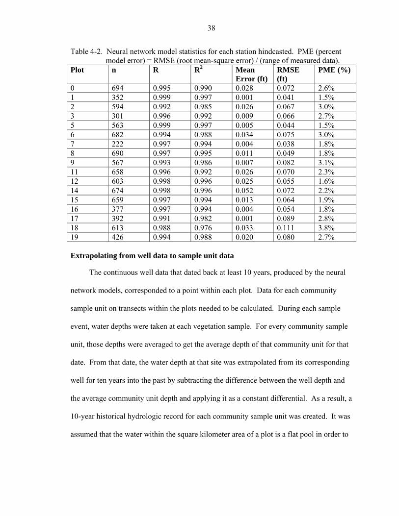
38

Table 4-2. Neural network model statistics for each station hindcasted. PME (percent model error) = RMSE (root mean-square error) / (range of measured data).

Plot n R R2 Mean Error (ft)

RMSE (ft)

PME (%)

0 694 0.995 0.990 0.028 0.072 2.6% 1 352 0.999 0.997 0.001 0.041 1.5% 2 594 0.992 0.985 0.026 0.067 3.0% 3 301 0.996 0.992 0.009 0.066 2.7% 5 563 0.999 0.997 0.005 0.044 1.5% 6 682 0.994 0.988 0.034 0.075 3.0% 7 222 0.997 0.994 0.004 0.038 1.8% 8 690 0.997 0.995 0.011 0.049 1.8% 9 567 0.993 0.986 0.007 0.082 3.1% 11 658 0.996 0.992 0.026 0.070 2.3% 12 603 0.998 0.996 0.025 0.055 1.6% 14 674 0.998 0.996 0.052 0.072 2.2% 15 659 0.997 0.994 0.013 0.064 1.9% 16 377 0.997 0.994 0.004 0.054 1.8% 17 392 0.991 0.982 0.001 0.089 2.8% 18 613 0.988 0.976 0.033 0.111 3.8% 19 426 0.994 0.988 0.020 0.080 2.7% Extrapolating from well data to sample unit data

The continuous well data that dated back at least 10 years, produced by the neural

network models, corresponded to a point within each plot. Data for each community

sample unit on transects within the plots needed to be calculated. During each sample

event, water depths were taken at each vegetation sample. For every community sample

unit, those depths were averaged to get the average depth of that community unit for that

date. From that date, the water depth at that site was extrapolated from its corresponding

well for ten years into the past by subtracting the difference between the well depth and

the average community unit depth and applying it as a constant differential. As a result, a

10-year historical hydrologic record for each community sample unit was created. It was

assumed that the water within the square kilometer area of a plot is a flat pool in order to

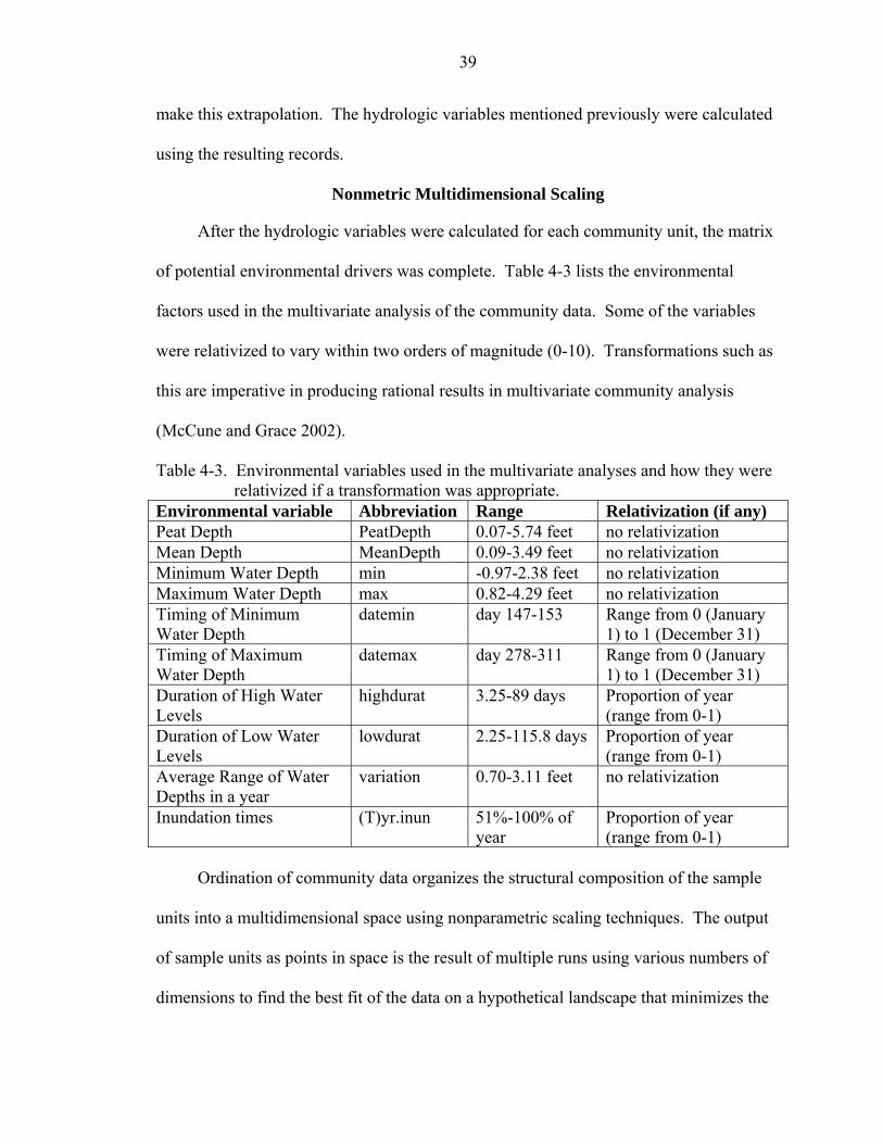
39

make this extrapolation. The hydrologic variables mentioned previously were calculated

using the resulting records.

Nonmetric Multidimensional Scaling

After the hydrologic variables were calculated for each community unit, the matrix

of potential environmental drivers was complete. Table 4-3 lists the environmental

factors used in the multivariate analysis of the community data. Some of the variables

were relativized to vary within two orders of magnitude (0-10). Transformations such as

this are imperative in producing rational results in multivariate community analysis

(McCune and Grace 2002).

Table 4-3. Environmental variables used in the multivariate analyses and how they were relativized if a transformation was appropriate.

Environmental variable Abbreviation Range Relativization (if any) Peat Depth PeatDepth 0.07-5.74 feet no relativization Mean Depth MeanDepth 0.09-3.49 feet no relativization Minimum Water Depth min -0.97-2.38 feet no relativization Maximum Water Depth max 0.82-4.29 feet no relativization Timing of Minimum Water Depth

datemin day 147-153 Range from 0 (January 1) to 1 (December 31)

Timing of Maximum Water Depth

datemax day 278-311 Range from 0 (January 1) to 1 (December 31)

Duration of High Water Levels

highdurat 3.25-89 days Proportion of year (range from 0-1)

Duration of Low Water Levels

lowdurat 2.25-115.8 days Proportion of year (range from 0-1)

Average Range of Water Depths in a year

variation 0.70-3.11 feet no relativization

Inundation times (T)yr.inun 51%-100% of year

Proportion of year (range from 0-1)

Ordination of community data organizes the structural composition of the sample

units into a multidimensional space using nonparametric scaling techniques. The output

of sample units as points in space is the result of multiple runs using various numbers of

dimensions to find the best fit of the data on a hypothetical landscape that minimizes the

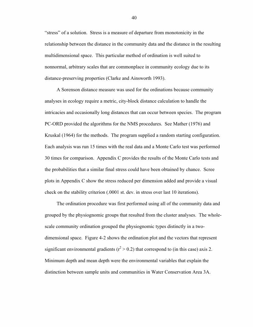
40

“stress” of a solution. Stress is a measure of departure from monotonicity in the

relationship between the distance in the community data and the distance in the resulting

multidimensional space. This particular method of ordination is well suited to

nonnormal, arbitrary scales that are commonplace in community ecology due to its

distance-preserving properties (Clarke and Ainsworth 1993).

A Sorenson distance measure was used for the ordinations because community

analyses in ecology require a metric, city-block distance calculation to handle the

intricacies and occasionally long distances that can occur between species. The program

PC-ORD provided the algorithms for the NMS procedures. See Mather (1976) and

Kruskal (1964) for the methods. The program supplied a random starting configuration.

Each analysis was run 15 times with the real data and a Monte Carlo test was performed

30 times for comparison. Appendix C provides the results of the Monte Carlo tests and

the probabilities that a similar final stress could have been obtained by chance. Scree

plots in Appendix C show the stress reduced per dimension added and provide a visual

check on the stability criterion (.0001 st. dev. in stress over last 10 iterations).

The ordination procedure was first performed using all of the community data and

grouped by the physiognomic groups that resulted from the cluster analyses. The whole-

scale community ordination grouped the physiognomic types distinctly in a two-

dimensional space. Figure 4-2 shows the ordination plot and the vectors that represent

significant environmental gradients (r2 > 0.2) that correspond to (in this case) axis 2.

Minimum depth and mean depth were the environmental variables that explain the

distinction between sample units and communities in Water Conservation Area 3A.

41

Figure 4-2. A whole scale ordination plot of the community sample units. Triangles

represent individual sample units and crosses represent species. The key to the legend: 1—prairie physiognomic type; 2—slough physiognomic type; 3—sawgrass physiognomic type; 4—island physiognomic type. The environmental gradients (minimum depth and mean depth) are represented with red vectors closely aligned with axis 2.

The ordination procedure was repeated using each of the physiognomic types

separately to attempt to discover the relationship between states of each physiognomic

type and the environment. Figure 4-3 is an ordination plot of island-type communities.

The three meta-stable states of island-types are best fit into a three-dimensional space.

Shown are ordination plots of axis 1 and axis 2 and a plot of axes 2 and 3, providing a

less than clear distinction between states of island-types. There is no correlation of

environmental variables to the ordination axes.

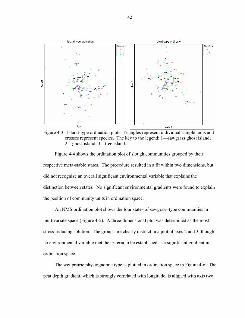
42

Figure 4-3. Island-type ordination plots. Triangles represent individual sample units and crosses represent species. The key to the legend: 1—sawgrass ghost island; 2—ghost island; 3—tree island.

Figure 4-4 shows the ordination plot of slough communities grouped by their

respective meta-stable states. The procedure resulted in a fit within two dimensions, but

did not recognize an overall significant environmental variable that explains the

distinction between states No significant environmental gradients were found to explain

the position of community units in ordination space.

An NMS ordination plot shows the four states of sawgrass-type communities in

multivariate space (Figure 4-5). A three-dimensional plot was determined as the most

stress-reducing solution. The groups are clearly distinct in a plot of axes 2 and 3, though

no environmental variable met the criteria to be established as a significant gradient in

ordination space.

The wet prairie physiognomic type is plotted in ordination space in Figure 4-6. The

peat depth gradient, which is strongly correlated with longitude, is aligned with axis two

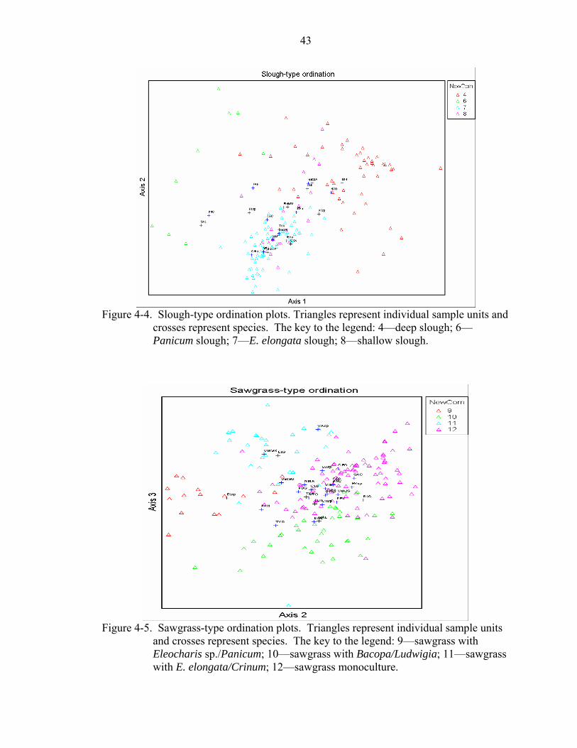
43

Figure 4-4. Slough-type ordination plots. Triangles represent individual sample units and

crosses represent species. The key to the legend: 4—deep slough; 6—Panicum slough; 7—E. elongata slough; 8—shallow slough.

Figure 4-5. Sawgrass-type ordination plots. Triangles represent individual sample units

and crosses represent species. The key to the legend: 9—sawgrass with Eleocharis sp./Panicum; 10—sawgrass with Bacopa/Ludwigia; 11—sawgrass with E. elongata/Crinum; 12—sawgrass monoculture.

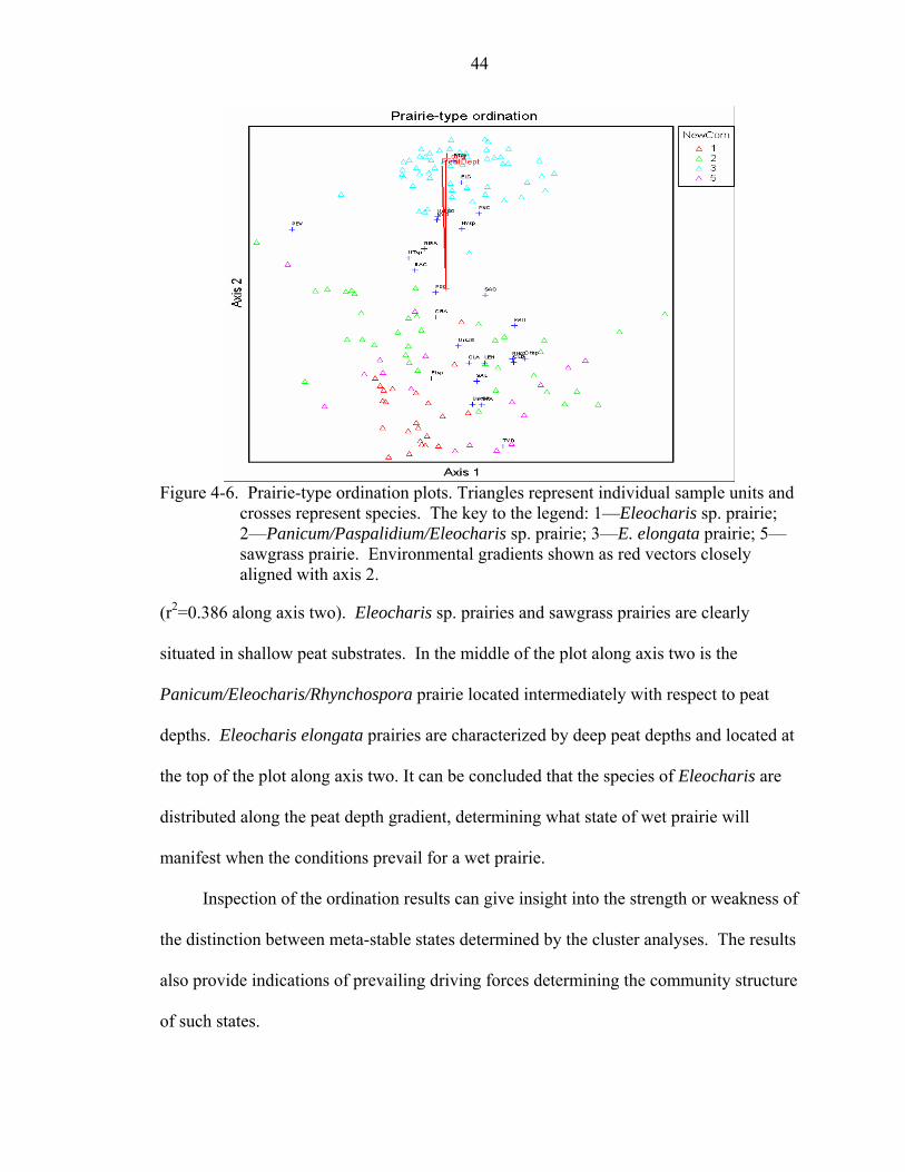
44

Figure 4-6. Prairie-type ordination plots. Triangles represent individual sample units and

crosses represent species. The key to the legend: 1—Eleocharis sp. prairie; 2—Panicum/Paspalidium/Eleocharis sp. prairie; 3—E. elongata prairie; 5—sawgrass prairie. Environmental gradients shown as red vectors closely aligned with axis 2.

(r2=0.386 along axis two). Eleocharis sp. prairies and sawgrass prairies are clearly

situated in shallow peat substrates. In the middle of the plot along axis two is the

Panicum/Eleocharis/Rhynchospora prairie located intermediately with respect to peat

depths. Eleocharis elongata prairies are characterized by deep peat depths and located at

the top of the plot along axis two. It can be concluded that the species of Eleocharis are

distributed along the peat depth gradient, determining what state of wet prairie will

manifest when the conditions prevail for a wet prairie.

Inspection of the ordination results can give insight into the strength or weakness of

the distinction between meta-stable states determined by the cluster analyses. The results

also provide indications of prevailing driving forces determining the community structure

of such states.

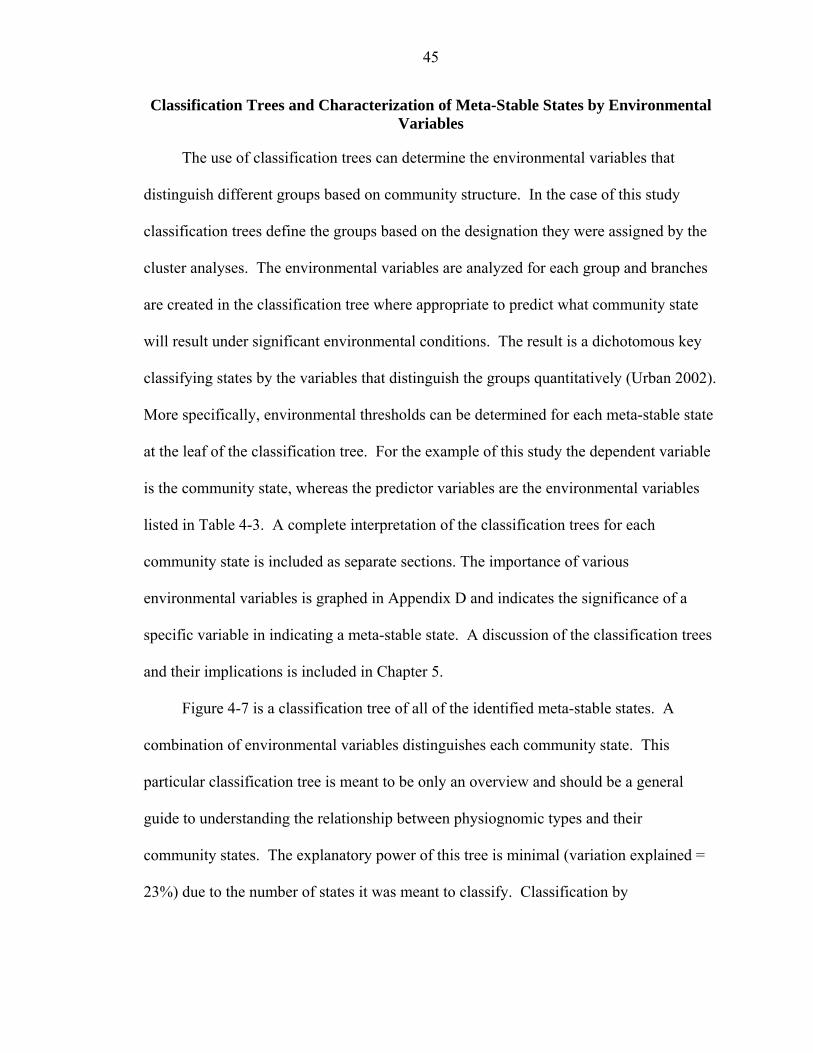
45

Classification Trees and Characterization of Meta-Stable States by Environmental Variables

The use of classification trees can determine the environmental variables that

distinguish different groups based on community structure. In the case of this study

classification trees define the groups based on the designation they were assigned by the

cluster analyses. The environmental variables are analyzed for each group and branches

are created in the classification tree where appropriate to predict what community state

will result under significant environmental conditions. The result is a dichotomous key

classifying states by the variables that distinguish the groups quantitatively (Urban 2002).

More specifically, environmental thresholds can be determined for each meta-stable state

at the leaf of the classification tree. For the example of this study the dependent variable

is the community state, whereas the predictor variables are the environmental variables

listed in Table 4-3. A complete interpretation of the classification trees for each

community state is included as separate sections. The importance of various

environmental variables is graphed in Appendix D and indicates the significance of a

specific variable in indicating a meta-stable state. A discussion of the classification trees

and their implications is included in Chapter 5.

Figure 4-7 is a classification tree of all of the identified meta-stable states. A

combination of environmental variables distinguishes each community state. This

particular classification tree is meant to be only an overview and should be a general

guide to understanding the relationship between physiognomic types and their

community states. The explanatory power of this tree is minimal (variation explained =

23%) due to the number of states it was meant to classify. Classification by

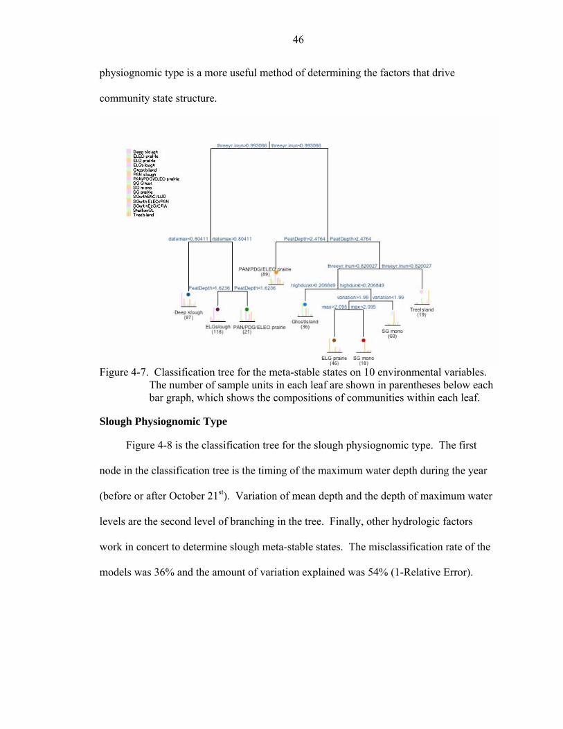
46

physiognomic type is a more useful method of determining the factors that drive

community state structure.

Figure 4-7. Classification tree for the meta-stable states on 10 environmental variables.

The number of sample units in each leaf are shown in parentheses below each bar graph, which shows the compositions of communities within each leaf.

Slough Physiognomic Type

Figure 4-8 is the classification tree for the slough physiognomic type. The first

node in the classification tree is the timing of the maximum water depth during the year

(before or after October 21st). Variation of mean depth and the depth of maximum water

levels are the second level of branching in the tree. Finally, other hydrologic factors

work in concert to determine slough meta-stable states. The misclassification rate of the

models was 36% and the amount of variation explained was 54% (1-Relative Error).

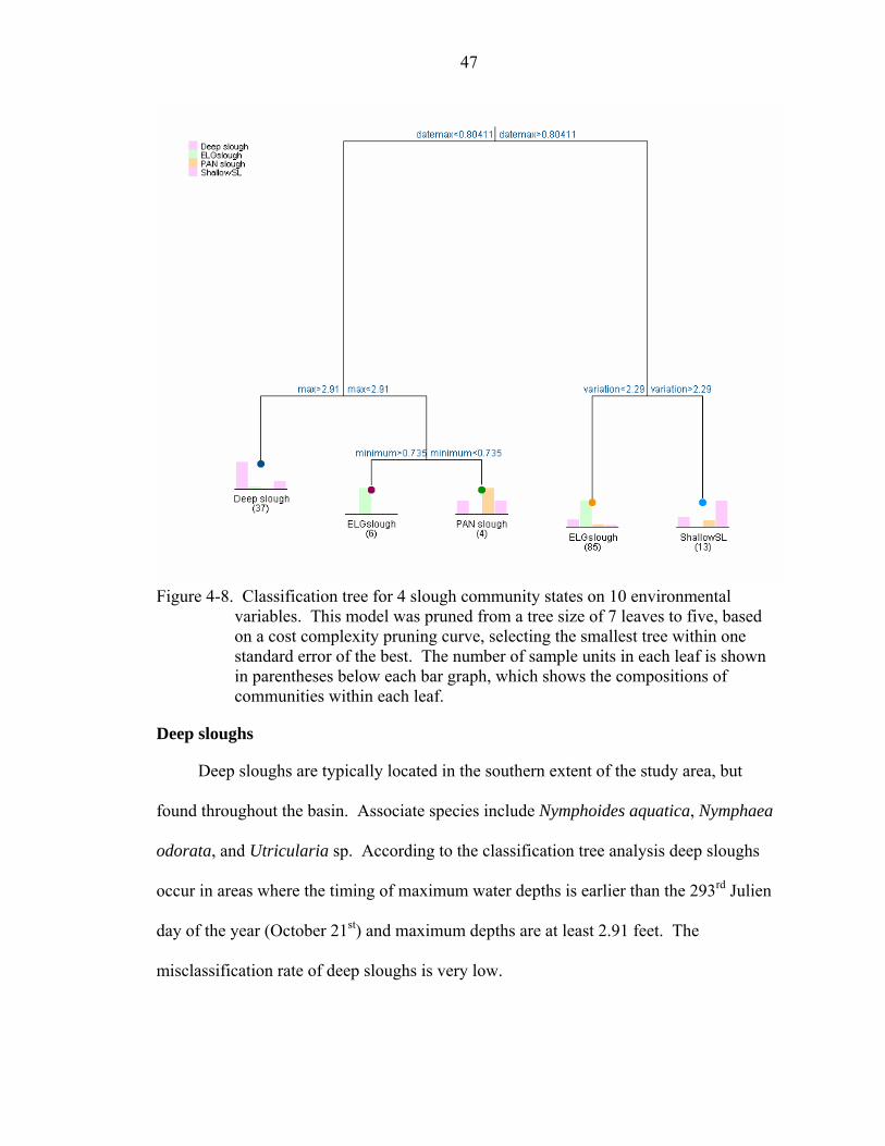
47

Figure 4-8. Classification tree for 4 slough community states on 10 environmental

variables. This model was pruned from a tree size of 7 leaves to five, based on a cost complexity pruning curve, selecting the smallest tree within one standard error of the best. The number of sample units in each leaf is shown in parentheses below each bar graph, which shows the compositions of communities within each leaf.

Deep sloughs

Deep sloughs are typically located in the southern extent of the study area, but

found throughout the basin. Associate species include Nymphoides aquatica, Nymphaea

odorata, and Utricularia sp. According to the classification tree analysis deep sloughs

occur in areas where the timing of maximum water depths is earlier than the 293rd Julien

day of the year (October 21st) and maximum depths are at least 2.91 feet. The

misclassification rate of deep sloughs is very low.

48

Eleocharis elongata sloughs

This particular slough community state occurs everywhere except in the

southeastern portion of the water conservation area, which is typified by deep peats, long

hydroperiods, and floating mats. Associate species of this community include Eleocharis

geniculata, Nymphaea odorata, Utricularia, and Hymenocallis. According to the

classification tree they occur where variation in water depths is less than 2.29 feet during

the year.

Panicum sloughs

Panicum hemitomon sloughs are mostly limited to the northwestern reaches of the

study area. Associate species of this community include Panicum hemitomon,

Paspalidium geminatum, and some of the typical slough species (N. odorata, N. aquatica,

and Utricularia). According to the classification tree this community state occurs in

relatively shallow site, requiring maximum water depths of less than 2.91 feet and

minimum water depths of less than 0.735 feet.

Shallow sloughs

Shallow sloughs are evenly distributed across the landscape. They consist of

mainly Utricularia, but associates may include P. hemitomon, P. geminatum, N. odorata,

and N. aquatica. According to the classification tree they prefer maximum depths late in

the year and occur in sites with greater variation in water depths throughout the year.

Wet Prairie Physiognomic Type

Figure 4-8 is the classification tree for the wet prairie physiognomic type. The first

node and most important explanatory variable distinguishing conditions in wet prairie

communities is peat depth. Duration of high water levels, hydroperiod, timing of

maximum water levels, duration of low water levels, hydroperiod and annual average of

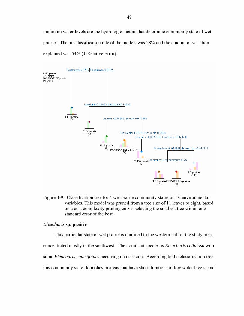
49

minimum water levels are the hydrologic factors that determine community state of wet

prairies. The misclassification rate of the models was 28% and the amount of variation

explained was 54% (1-Relative Error).

Figure 4-9. Classification tree for 4 wet prairie community states on 10 environmental

variables. This model was pruned from a tree size of 11 leaves to eight, based on a cost complexity pruning curve, selecting the smallest tree within one standard error of the best.

Eleocharis sp. prairie

This particular state of wet prairie is confined to the western half of the study area,

concentrated mostly in the southwest. The dominant species is Eleocharis cellulosa with

some Eleocharis equisifoides occurring on occasion. According to the classification tree,

this community state flourishes in areas that have short durations of low water levels, and

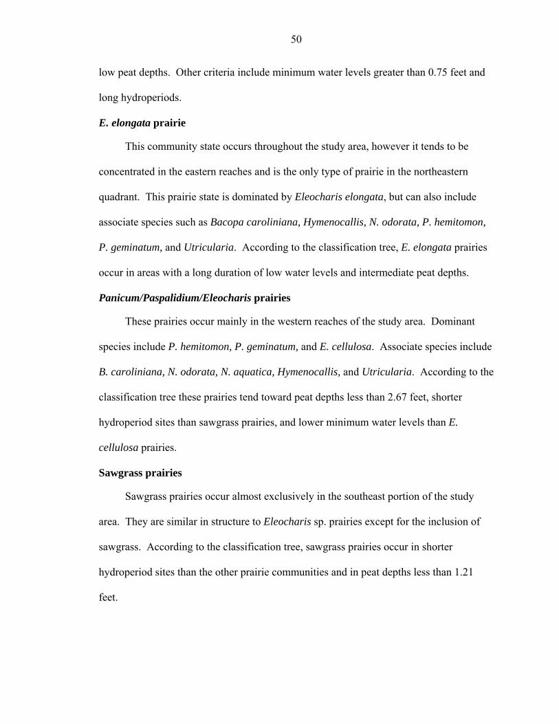
50

low peat depths. Other criteria include minimum water levels greater than 0.75 feet and

long hydroperiods.

E. elongata prairie

This community state occurs throughout the study area, however it tends to be

concentrated in the eastern reaches and is the only type of prairie in the northeastern

quadrant. This prairie state is dominated by Eleocharis elongata, but can also include

associate species such as Bacopa caroliniana, Hymenocallis, N. odorata, P. hemitomon,

P. geminatum, and Utricularia. According to the classification tree, E. elongata prairies

occur in areas with a long duration of low water levels and intermediate peat depths.

Panicum/Paspalidium/Eleocharis prairies

These prairies occur mainly in the western reaches of the study area. Dominant

species include P. hemitomon, P. geminatum, and E. cellulosa. Associate species include

B. caroliniana, N. odorata, N. aquatica, Hymenocallis, and Utricularia. According to the

classification tree these prairies tend toward peat depths less than 2.67 feet, shorter

hydroperiod sites than sawgrass prairies, and lower minimum water levels than E.

cellulosa prairies.

Sawgrass prairies

Sawgrass prairies occur almost exclusively in the southeast portion of the study

area. They are similar in structure to Eleocharis sp. prairies except for the inclusion of

sawgrass. According to the classification tree, sawgrass prairies occur in shorter

hydroperiod sites than the other prairie communities and in peat depths less than 1.21

feet.

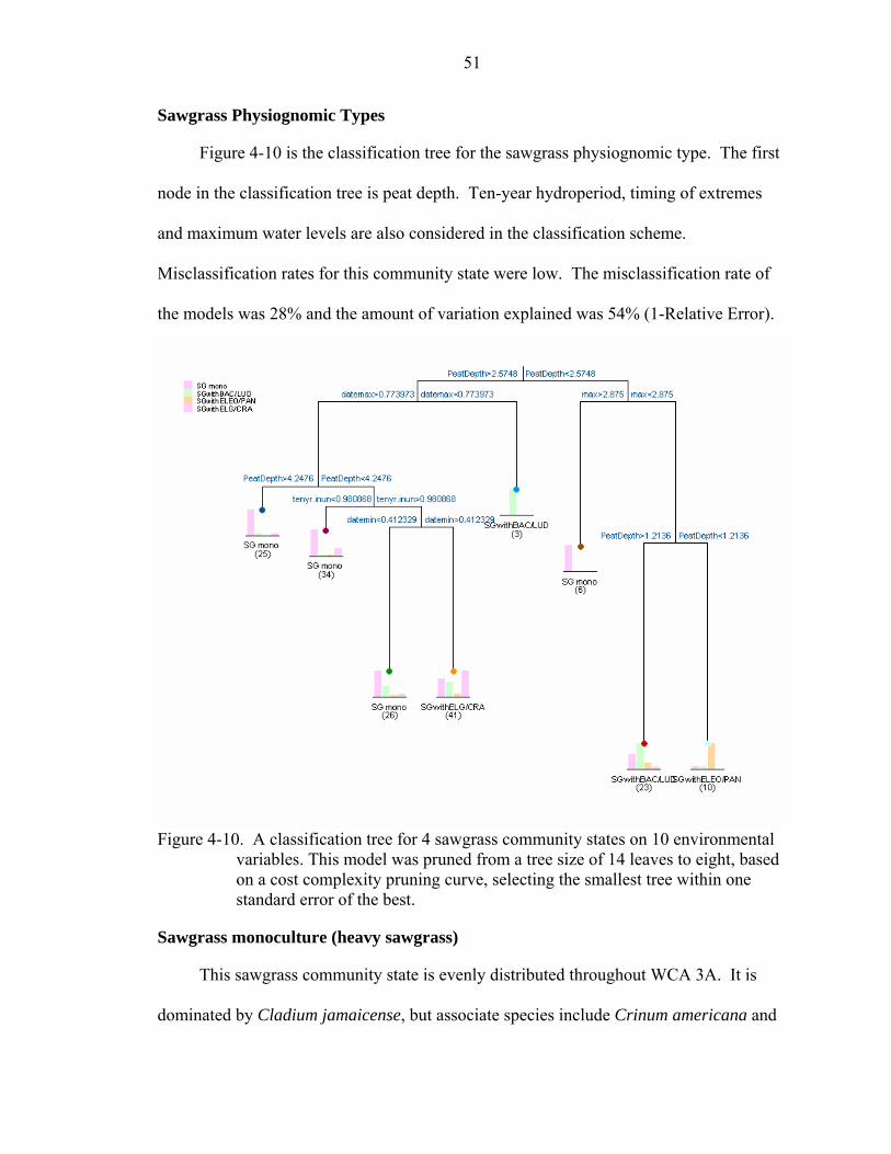
51

Sawgrass Physiognomic Types

Figure 4-10 is the classification tree for the sawgrass physiognomic type. The first

node in the classification tree is peat depth. Ten-year hydroperiod, timing of extremes

and maximum water levels are also considered in the classification scheme.

Misclassification rates for this community state were low. The misclassification rate of

the models was 28% and the amount of variation explained was 54% (1-Relative Error).

Figure 4-10. A classification tree for 4 sawgrass community states on 10 environmental

variables. This model was pruned from a tree size of 14 leaves to eight, based on a cost complexity pruning curve, selecting the smallest tree within one standard error of the best.

Sawgrass monoculture (heavy sawgrass)

This sawgrass community state is evenly distributed throughout WCA 3A. It is

dominated by Cladium jamaicense, but associate species include Crinum americana and

52

Ludwigia spp. According to the classification tree, heavy sawgrass communities are well

distributed across all conditions. Heavy sawgrass is generally found in deeper peat.

Sawgrass with Bacopa and Ludwigia

This state of sawgrass occurs throughout the study area, but is concentrated in the

southwest reaches. Typical species include sawgrass and B. caroliniana. Associate

species include Ludwigia spp. and C. Americana. According to the classification tree,

this community state occurs in peat depths ranging from 1.2 ft to 2.6 ft. Maximum water

levels should remain under 2.9 ft.

Sawgrass with Eleocharis sp. and Panicum

The sawgrass with Eleocharis and Panicum state occurs throughout the study area

except for the southeastern quadrant. This community state is dominated by sawgrass

and Eleocharis sp. Associate species include P. hemitomon, P. geminatum, Typha sp.

and Leersia hexandra. According to the classification tree, this state occurs in peat

depths of less than 1.2 ft and maximum water levels that remain under 2.9 ft.

Sawgrass with E. elongata and Crinum

This community occurs throughout the study area, yet is rarely found in the

southeastern quadrant. A diverse community state, dominant species include sawgrass,

E. elongata, and C. americana. Associate species include B. caroliniana, Cephalanthus

occidentalis, Hymenocallis, L. hexandra, Peltandra virginica, Pontederia cordata,

Ludwigia sp., and E. equistifoides. According to the classification tree, this community

state occurs in peat depths that are between 2.6 ft and 4.2 ft, and relatively long

hydroperiods compared to heavy sawgrass. Timing of extreme water levels should occur

later in the year.

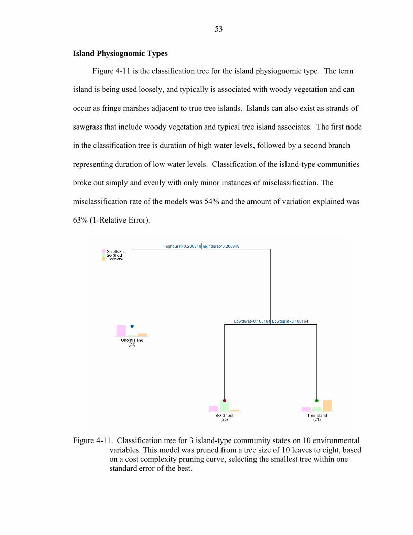
53

Island Physiognomic Types

Figure 4-11 is the classification tree for the island physiognomic type. The term

island is being used loosely, and typically is associated with woody vegetation and can

occur as fringe marshes adjacent to true tree islands. Islands can also exist as strands of

sawgrass that include woody vegetation and typical tree island associates. The first node

in the classification tree is duration of high water levels, followed by a second branch

representing duration of low water levels. Classification of the island-type communities

broke out simply and evenly with only minor instances of misclassification. The

misclassification rate of the models was 54% and the amount of variation explained was

63% (1-Relative Error).

Figure 4-11. Classification tree for 3 island-type community states on 10 environmental

variables. This model was pruned from a tree size of 10 leaves to eight, based on a cost complexity pruning curve, selecting the smallest tree within one standard error of the best.

54

Ghost islands

The ghost island community state occurs throughout the study area. Dominant

species include P. virginica, P. cordata, and C. occidentalis. Associate species include

Crinum, Ludwigia, Sagittaria lancifolia, and sawgrass. According to the classification

tree, ghost island communities require durations of high water levels for over 20% of the

year.

Sawgrass ghost islands

This community state occurs throughout the study area except in the northwest

quadrant. Sawgrass ghost islands are dominated by sawgrass, L. hexandra, P. virginica,

S. lancifolia, and C. occidentalis. Associate species include P. cordata, Blechnum

serrulatum, and Ludwigia sp. According to the classification tree, these communities

prefer durations of high water less than 20% of the year and durations of low water

greater than 10% of the year.

Tree islands

This community state occurs throughout the study area except in the southeast.

Due to the low number of samples however, this community probably occurs in all

quadrants of the study area. The dominant species are the ferns Osmunda regalis, and B.

serrulatum. Typical associates are Ludwigia, Typha, S. lancifolia, P. cordata, C.

occidentalis, and sawgrass. According to the classification tree, tree island communities

occur in areas where duration of high water levels is less than 20% of the year and

duration of low water levels is less than 10% of the year.

55

CHAPTER 5 SUMMARY AND CONCLUSIONS

Discussion

This thesis examines community-scale vegetation dynamics across the landscape-

level processes and drivers of Water Conservation Area 3A, of the Everglades.

Hydrologic processes vary seasonally and annually, but leave legacies that last years or

decades. The other processes that were examined operate on the temporal scale of

decades, such as soil accretion and erosion. Some of the processes examined are

anthropogenically influenced as well as driven by weather patterns. Vegetative

communities respond differentially to these drivers, and comprehension of how

communities respond is essential to management and restoration efforts.

Decompartmentalization and reorganization of the hydroscape for restoration purposes

illustrates the need to grasp the intricacies of community dynamics in the Everglades.

Only through the understanding of how the major drivers of the landscape operate, can

decision-makers rationalize a truly bottom-up approach to management of such a unique

and complex system of habitat and wildlife. Models based on a few key environmental

variables can be valuable tools in conservation management of dynamic wetlands (Toner

and Keddy 1997). This study provides the next step in the identification of those

variables and how they influence community structure.

Identification of meta-stable states of communities is essential for examination of

whole-scale community dynamics. Processes may have only subtle effects on

community structure over a short period of time. These subtleties can provide clues as to

56

the drivers that are causing potential shifts in landscape-level configurations of

vegetation. Chapter 3 identifies the meta-stable states of marsh physiognomic types of

WCA 3A, using a hierarchical clustering technique to analyze the community data

monitored semiannually over two years. Appendix B provides the structural signature of

each of these states. Four slough states were identified: deep slough, shallow slough,

Panicum slough, and Eleocharis elongata slough. Prairie communities manifest as four

different states: Eleocharis sp. prairie, Panicum/Paspalidium/Eleocharis prairie, E.

elongata prairie, and sawgrass prairie. Four states of the sawgrass physiognomic type

were identified: sawgrass with Eleocharis/Panicum, sawgrass with Bacopa/Ludwigia,

sawgrass with E. elongata/Crinum, and heavy sawgrass. Finally, shrubby marsh

communities, noted in this thesis as island-types, manifest as three different states:

sawgrass ghost island, ghost island, and tree island.

The majority of analyses performed on the data collected were multivariate in

approach due to the complex interactions and combinations of environmental variables

working in concert to create a unique, dense matrix of conditions in the study area.

Community ecology is best studied in a multivariate framework because of the

complexities of ecological interactions. Univariate comparisons, however, can be useful

in discovering basic trends in distributions of communities across a single gradient.

Figure 5-1 plots the mean water depths of the meta-stable states identified by the cluster

analyses. The chart illustrates both how slight the differentiation, as well as the

distinctive differences of hydrologic factors are between physiognomic types and

community states are. Deep slough and E. elongata slough states are the deepest of the

communities, though they also persist in a relatively wide range of hydroperiods. The E.

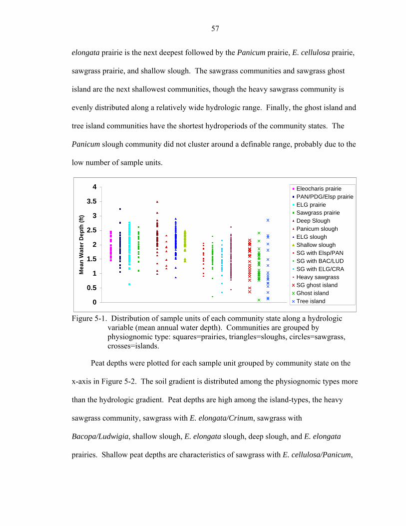
57

elongata prairie is the next deepest followed by the Panicum prairie, E. cellulosa prairie,

sawgrass prairie, and shallow slough. The sawgrass communities and sawgrass ghost

island are the next shallowest communities, though the heavy sawgrass community is

evenly distributed along a relatively wide hydrologic range. Finally, the ghost island and

tree island communities have the shortest hydroperiods of the community states. The

Panicum slough community did not cluster around a definable range, probably due to the

low number of sample units.

0

0.5

1

1.5

2

2.5

3

3.5

4

Mea

n W

ater

Dep

th (f

t)

Eleocharis prairiePAN/PDG/Elsp prairieELG prairieSawgrass prairieDeep SloughPanicum sloughELG sloughShallow sloughSG with Elsp/PANSG with BAC/LUDSG with ELG/CRAHeavy sawgrassSG ghost islandGhost islandTree island

Figure 5-1. Distribution of sample units of each community state along a hydrologic

variable (mean annual water depth). Communities are grouped by physiognomic type: squares=prairies, triangles=sloughs, circles=sawgrass, crosses=islands.

Peat depths were plotted for each sample unit grouped by community state on the

x-axis in Figure 5-2. The soil gradient is distributed among the physiognomic types more

than the hydrologic gradient. Peat depths are high among the island-types, the heavy

sawgrass community, sawgrass with E. elongata/Crinum, sawgrass with

Bacopa/Ludwigia, shallow slough, E. elongata slough, deep slough, and E. elongata

prairies. Shallow peat depths are characteristics of sawgrass with E. cellulosa/Panicum,

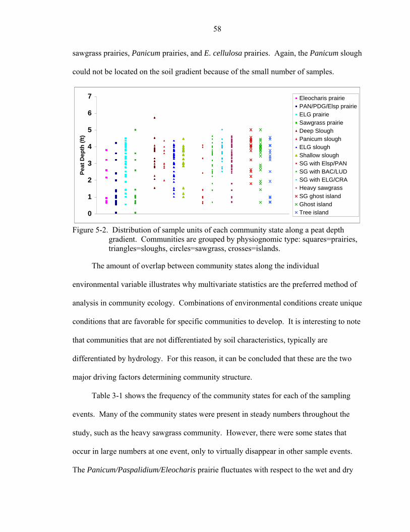
58

sawgrass prairies, Panicum prairies, and E. cellulosa prairies. Again, the Panicum slough

could not be located on the soil gradient because of the small number of samples.

0

1

2

3

4

5

6

7

Peat

Dep

th (f

t)

Eleocharis prairiePAN/PDG/Elsp prairieELG prairieSawgrass prairieDeep SloughPanicum sloughELG sloughShallow sloughSG with Elsp/PANSG with BAC/LUDSG with ELG/CRAHeavy sawgrassSG ghost islandGhost islandTree island

Figure 5-2. Distribution of sample units of each community state along a peat depth

gradient. Communities are grouped by physiognomic type: squares=prairies, triangles=sloughs, circles=sawgrass, crosses=islands.

The amount of overlap between community states along the individual

environmental variable illustrates why multivariate statistics are the preferred method of

analysis in community ecology. Combinations of environmental conditions create unique

conditions that are favorable for specific communities to develop. It is interesting to note

that communities that are not differentiated by soil characteristics, typically are

differentiated by hydrology. For this reason, it can be concluded that these are the two

major driving factors determining community structure.

Table 3-1 shows the frequency of the community states for each of the sampling

events. Many of the community states were present in steady numbers throughout the

study, such as the heavy sawgrass community. However, there were some states that

occur in large numbers at one event, only to virtually disappear in other sample events.

The Panicum/Paspalidium/Eleocharis prairie fluctuates with respect to the wet and dry

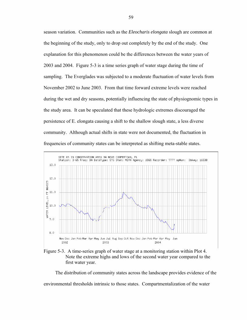
59

season variation. Communities such as the Eleocharis elongata slough are common at

the beginning of the study, only to drop out completely by the end of the study. One

explanation for this phenomenon could be the differences between the water years of

2003 and 2004. Figure 5-3 is a time series graph of water stage during the time of

sampling. The Everglades was subjected to a moderate fluctuation of water levels from

November 2002 to June 2003. From that time forward extreme levels were reached

during the wet and dry seasons, potentially influencing the state of physiognomic types in

the study area. It can be speculated that these hydrologic extremes discouraged the

persistence of E. elongata causing a shift to the shallow slough state, a less diverse

community. Although actual shifts in state were not documented, the fluctuation in

frequencies of community states can be interpreted as shifting meta-stable states.

Figure 5-3. A time-series graph of water stage at a monitoring station within Plot 4.

Note the extreme highs and lows of the second water year compared to the first water year.

The distribution of community states across the landscape provides evidence of the

environmental thresholds intrinsic to those states. Compartmentalization of the water

60

conservation areas creates a relatively flat hydroscape to the elevational gradient. The

same physiognomic types are exposed to differential hydroperiods, depending on their

position along a north-south axis. Soil types and characteristics vary along a longitudinal

axis, with shallow peat depths in the west and deep peat depths to the east. Figure 3-6 is

a graphical representation of the distribution of community states across the landscape. It

is apparent through examination of the community distribution figure that species such as

Panicum hemitomon and E. cellulosa are endemic to areas within the region that parallel

environmental requirements for those species. P. hemitomon is almost exclusively

located in the northern reaches of the study area where shorter hydroperiods persist.

Prairies dominated by E. cellulosa are confined to the western reaches where shallow

peats are typical. The scale of the study allows observation of the range of communities

and environmental conditions within WCA 3A.

An investigation of the environmental conditions of each of these community states

offers insight as to how they are related in terms of successional order and environmental

thresholds. When variables that influence the state of a physiognomic type are identified,

they can be quantified using classification trees. Thresholds of hydrologic variation and

extremes are discovered and a picture of where meta-stable states lie on the continuum of

a multidimensional environmental space begins to emerge. Relative positions of

physiognomic types in this space are already common knowledge to ecologists. In order

of short to long hydroperiod communities, the sequence goes: island, sawgrass, prairie,

slough. The evidence presented through this study shows some overlap in hydrology

between these physiognomic types, though the basic relationships remain.

61

The classification tree analyses in Chapter 4 describe how the community states

identified by the clustering techniques break out in terms of environmental conditions.

Slough communities were determined by hydrologic factors such as timing of maximum

water depths and the magnitude of extreme water levels. Deep slough communities

require early timing of maximum water levels. Early timing of water levels suggests

location further to the north where there is little time lag compared to the southern extent

of the conservation area where water tends to pile up later along Tamiami Trail.

However, high maximum water levels are required to drown out typical slough associates

like Panicum hemitomon. Panicum sloughs favor shorter hydroperiod sites, as revealed

by the classification tree. E. elongata sloughs favor late timing and minimal variation of

water depths, whereas shallow sloughs tolerate a wide range of water depths. The

implications for this could mean that Eleocharis elongata, as a species, may be less

resilient and more sensitive to hydrologic disturbance. Shallow sloughs tend to be less

diverse, so in the event of massive variation between seasons, E. elongata sloughs could

convert into a shallow slough state.

Peat depth was the major determinant for wet prairie meta-stable states. A close

inspection of the classification tree reveals that E. elongata prairies tend to persist in deep

peat depths and relatively long duration of lower water levels. Confined mostly toward

the eastern half of the study area, this prairie state occurs where soil conditions are

conducive for its establishment. Eleocharis sp. prairies, on the other hand, prefer shallow

peats, which are typical of the western reaches of the study area. Sawgrass prairies have

similar requirements as Eleocharis prairies, but tend towards shorter hydroperiod sites.

62

Finally Panicum/Paspalidium/Eleocharis prairies lack a restrictive soil requirement, but

prefer even shorter hydroperiod sites than sawgrass prairies.

In the cluster analyses sawgrass units were grouped mainly by diversity. Heavy

sawgrass states were fairly common. The classification tree analysis reveals that heavy

sawgrass is ubiquitous throughout the study area and occupies the range of environmental

conditions that are characteristic of the sawgrass physiognomic type. Sawgrass with

Bacopa/Ludwigia occur in shorter hydroperiod sites. Also occupying short hydroperiod

sites is the sawgrass with Eleocharis/Panicum state, yet it is confined to areas of shallow

peats, as are most Eleocharis cellulosa associated communities. Sawgrass with E.

elongata/Crinum communities prefer areas of long hydroperiods and deep peat depths.

This community state is probably the sparse sawgrass communities of the southeastern

WCA 3A. These tall sawgrass communities are exposed to continuous inundation and

recruitment of sawgrass individuals is nonexistent. The resilience of these communities

is evident, as these conditions have prevailed for years. However, they are slowly being

replaced by some prairie and primarily slough associates in the absence of drawdown

events.

Island-type communities were determined entirely by duration of high and low

water events. The duration of annual extreme water level conditions has implications on

the balance of competitive and stress-tolerant organisms, as well as anaerobic stress in

plants. Ghost islands characterized by arrowheads and woody shrubs prefer high

duration of water levels. This may suggest they are or have been subject to soil

subsidence or oxidation. Long duration of low water levels is required for sawgrass

ghost islands, which may be old tree islands with slightly higher water levels, or sawgrass

63

ridges that have been colonized by woody shrubs for one reason or another. The tree

island community state is classified as a community that prefers short durations of

extreme water levels in general. This may suggest that tree islands are not resilient to

shifts in hydrologic regime and require minimal annual variation of water levels.

Comparing NMS and Classification Tree Techniques

One interesting observation worth discussion is the fact that the NMS ordination

joint plots for each of the physiognomic types did not reveal relationships to

environmental variables (except for the prairies). The ordination of the physiognomic

types confirmed what we know about the relationships between them. Hydrology is

clearly the factor determining physiognomic type. When the NMS ordination did not

reveal the same relationship between meta-stable states, it was somewhat surprising.

However, the ordination plots did show distinct patterns that distinguish the meta-stable

states from each other in species space.

The classification tree analyses interpret groups using the environmental variables

given. In this case, the meta-stable states are classified by the variables that distinguish

them. Misclassification is common and overfitting the data could be an issue. The

interpretability of the classification trees, however, provide insight into the conditions

that may be distinguishing the community states. The diversity of variables that were

determined to be associated with each physiognomic type outlines the complexity of

environmental variation between the meta-stable states. This may explain why individual

variables were not determined to be explanatory to structural variation in the NMS.

Perhaps the creation of an alternative metric that accounts for the variables determined by

the classification tree would be useful including in the ordination procedure.

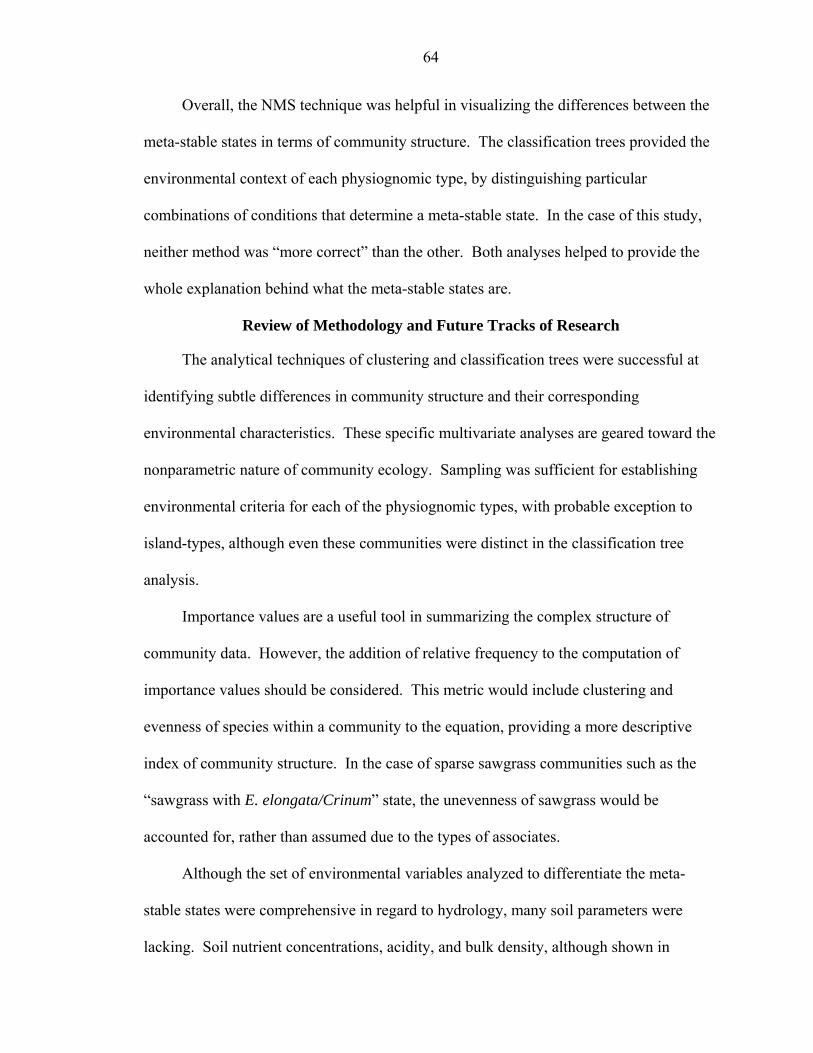
64

Overall, the NMS technique was helpful in visualizing the differences between the

meta-stable states in terms of community structure. The classification trees provided the

environmental context of each physiognomic type, by distinguishing particular

combinations of conditions that determine a meta-stable state. In the case of this study,

neither method was “more correct” than the other. Both analyses helped to provide the

whole explanation behind what the meta-stable states are.

Review of Methodology and Future Tracks of Research

The analytical techniques of clustering and classification trees were successful at

identifying subtle differences in community structure and their corresponding

environmental characteristics. These specific multivariate analyses are geared toward the

nonparametric nature of community ecology. Sampling was sufficient for establishing

environmental criteria for each of the physiognomic types, with probable exception to

island-types, although even these communities were distinct in the classification tree

analysis.

Importance values are a useful tool in summarizing the complex structure of

community data. However, the addition of relative frequency to the computation of

importance values should be considered. This metric would include clustering and

evenness of species within a community to the equation, providing a more descriptive

index of community structure. In the case of sparse sawgrass communities such as the

“sawgrass with E. elongata/Crinum” state, the unevenness of sawgrass would be

accounted for, rather than assumed due to the types of associates.

Although the set of environmental variables analyzed to differentiate the meta-

stable states were comprehensive in regard to hydrology, many soil parameters were

lacking. Soil nutrient concentrations, acidity, and bulk density, although shown in

65

previous studies to be uniform on a landscape scale in WCA 3A (given sufficient distance

from point sources i.e. canals, etc.), could be a factor in “hot spots” of wildlife activity.

Alligator holes and bird roosts tend to alter local soil chemistry characteristics.

Expansion of community dynamic studies in the Everglades should consider landscape

geometry and proximity to seed banks. It was not necessary to include these landscape

metrics in this study, because all of the research was located in one impounded section of

the Everglades that is relatively distant from disturbed upland habitat that would provide

a source of ruderal recruitment.

Future research should include the investigation of the “movement” of individual

sample units over time. NMS is a useful tool for quantifying and visualizing the

trajectory of a sample in species space. Coupled with changes in seasonal environmental

conditions, additional insights could be made into landscape level trends of community

shifts. Inferences into the resilience of community states could be made through NMS or

Multiresponse Permutational Procedures (MRPP) of individual sample units. Long-term

studies should monitor the movement of ecotones relative to hydrologic dynamics.

Reduction of the Everglades ecosystem to half of its size, loss of sheetflow through

the system, and loss of habitat diversity are some of the functional losses due to human

engineering efforts of the mid-20th century (Davis et al. 1994). Monitoring and

predicting landscape-scale vegetation dynamics is essential to the restoration efforts. The

potential for community dynamic research using the concepts of meta-stable states is

considerable. An adaptive management approach to Everglades restoration means that

hydrologic regimes will continue to change along with management strategies. The need

for greater understanding of the implications of future scenarios, will at the same time

66

allow researchers to further examination of the intricacies of Everglades community

dynamics.

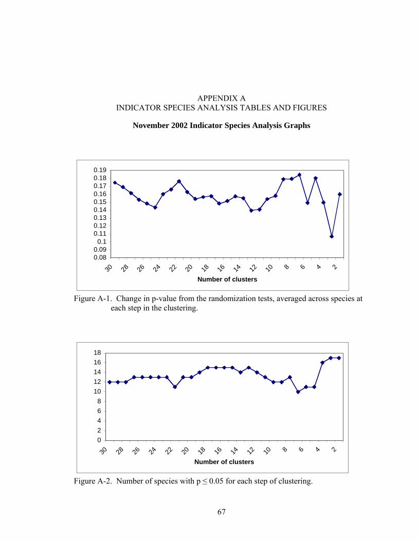
67

APPENDIX A INDICATOR SPECIES ANALYSIS TABLES AND FIGURES

November 2002 Indicator Species Analysis Graphs

0.080.09

0.10.110.120.130.140.150.160.170.180.19

30 28 26 24 22 20 18 16 14 12 10 8 6 4 2

Number of clusters

Figure A-1. Change in p-value from the randomization tests, averaged across species at

each step in the clustering.

02468

1012141618

30 28 26 24 22 20 18 16 14 12 10 8 6 4 2

Number of clusters

Figure A-2. Number of species with p ≤ 0.05 for each step of clustering.

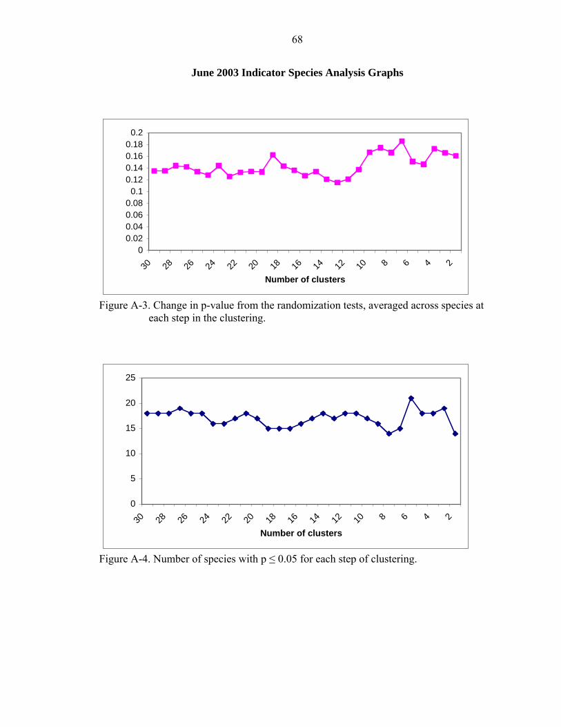
68

June 2003 Indicator Species Analysis Graphs

00.020.040.060.08

0.10.120.140.160.18

0.2

30 28 26 24 22 20 18 16 14 12 10 8 6 4 2

Number of clusters

Figure A-3. Change in p-value from the randomization tests, averaged across species at

each step in the clustering.

0

5

10

15

20

25

30 28 26 24 22 20 18 16 14 12 10 8 6 4 2

Number of clusters

Figure A-4. Number of species with p ≤ 0.05 for each step of clustering.

69

November 2003 Indicator Species Analysis Graphs

0.1

0.110.12

0.130.14

0.150.16

0.170.18

0.19

30 28 26 24 22 20 18 16 14 12 10 8 6 4 2

Figure A-5. Change in p-value from the randomization tests, averaged across species at

each step in the clustering.

02468

101214161820

30 29 28 27 26 25 24 23 22 21 20 19 18 17 16 15 14 13 12 11 10 9 8 7 6 5 4 3 2

Number of clusters

Figure A-6. Number of species with p ≤ 0.05 for each step of clustering.

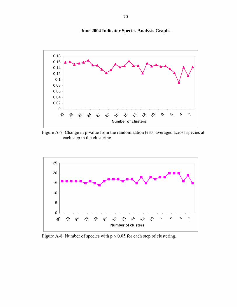
70

June 2004 Indicator Species Analysis Graphs

00.020.040.060.080.1

0.120.140.160.18

30 28 26 24 22 20 18 16 14 12 10 8 6 4 2

Number of clusters

Figure A-7. Change in p-value from the randomization tests, averaged across species at

each step in the clustering.

0

5

10

15

20

25

30 28 26 24 22 20 18 16 14 12 10 8 6 4 2

Number of clusters

Figure A-8. Number of species with p ≤ 0.05 for each step of clustering.

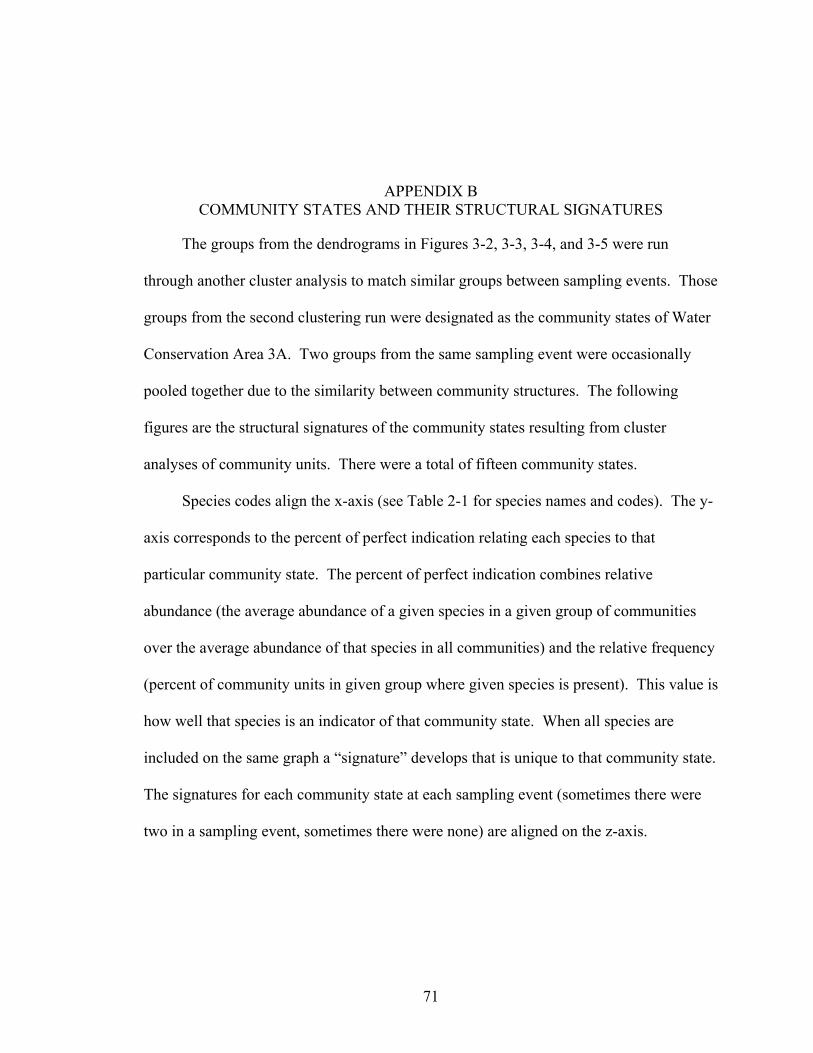
71

APPENDIX B COMMUNITY STATES AND THEIR STRUCTURAL SIGNATURES

The groups from the dendrograms in Figures 3-2, 3-3, 3-4, and 3-5 were run

through another cluster analysis to match similar groups between sampling events. Those

groups from the second clustering run were designated as the community states of Water

Conservation Area 3A. Two groups from the same sampling event were occasionally

pooled together due to the similarity between community structures. The following

figures are the structural signatures of the community states resulting from cluster

analyses of community units. There were a total of fifteen community states.

Species codes align the x-axis (see Table 2-1 for species names and codes). The y-

axis corresponds to the percent of perfect indication relating each species to that

particular community state. The percent of perfect indication combines relative

abundance (the average abundance of a given species in a given group of communities

over the average abundance of that species in all communities) and the relative frequency

(percent of community units in given group where given species is present). This value is

how well that species is an indicator of that community state. When all species are

included on the same graph a “signature” develops that is unique to that community state.

The signatures for each community state at each sampling event (sometimes there were

two in a sampling event, sometimes there were none) are aligned on the z-axis.

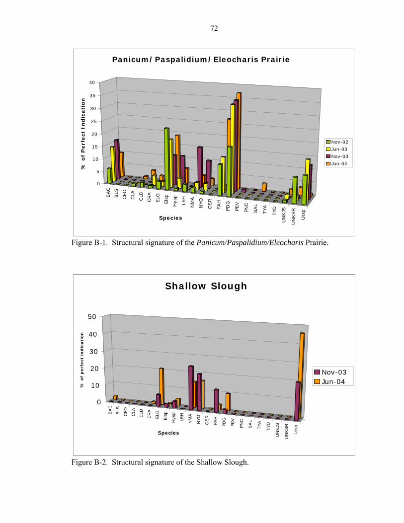
72

BA

C

BLS

CE

O

CLA

CLD

CR

A

ELG

Els

p

Hys

p

LEH

NM

A

NY

O

OS

R

PAH

PD

G

PEV

PNC

SA

L

TY

A

TY

D

UN

KJS

UN

KS

R

Uts

p

0

5

10

15

20

25

30

35

40%

of

Perf

ect

In

dic

ati

on

Species

Panicum/Paspalidium/Eleocharis Prairie

Nov-02

Jun-03

Nov-03

Jun-04

Figure B-1. Structural signature of the Panicum/Paspalidium/Eleocharis Prairie.

BA

C

BLS

CE

O

CLA

CLD

CR

A

ELG

Els

p

Hys

p

LEH

NM

A

NY

O

OS

R

PAH

PDG

PEV

PNC

SA

L

TY

A

TY

D

UN

KJS

UN

KS

R

Uts

p

0

10

20

30

40

50

% o

f p

erf

ect

in

dic

ati

on

Species

Shallow Slough

Nov-03Jun-04

Figure B-2. Structural signature of the Shallow Slough.

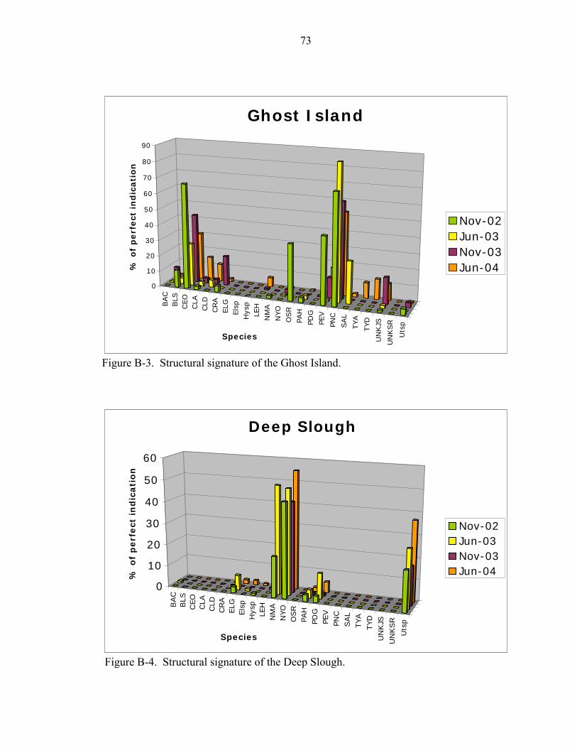
73

BA

CB

LSC

EO

CLA

CLD

CR

AE

LGE

lsp

Hys

pLE

HN

MA

NY

O

OS

R

PAH

PDG

PEV

PNC

SA

L

TY

A

TY

D

UN

KJS

UN

KS

R

Uts

p

0

10

20

30

40

50

60

70

80

90

% o

f p

erf

ect

in

dic

ati

on

Species

Ghost Island

Nov-02Jun-03Nov-03Jun-04

Figure B-3. Structural signature of the Ghost Island.

BA

CB

LSC

EO

CLA

CLD

CR

AE

LGE

lsp

Hys

pLE

HN

MA

NY

OO

SR

PAH

PD

GP

EV

PN

CS

AL

TY

AT

YD

UN

KJS

UN

KS

R

Uts

p

0

10

20

30

40

50

60

% o

f p

erf

ect

in

dic

ati

on

Species

Deep Slough

Nov-02Jun-03Nov-03Jun-04

Figure B-4. Structural signature of the Deep Slough.

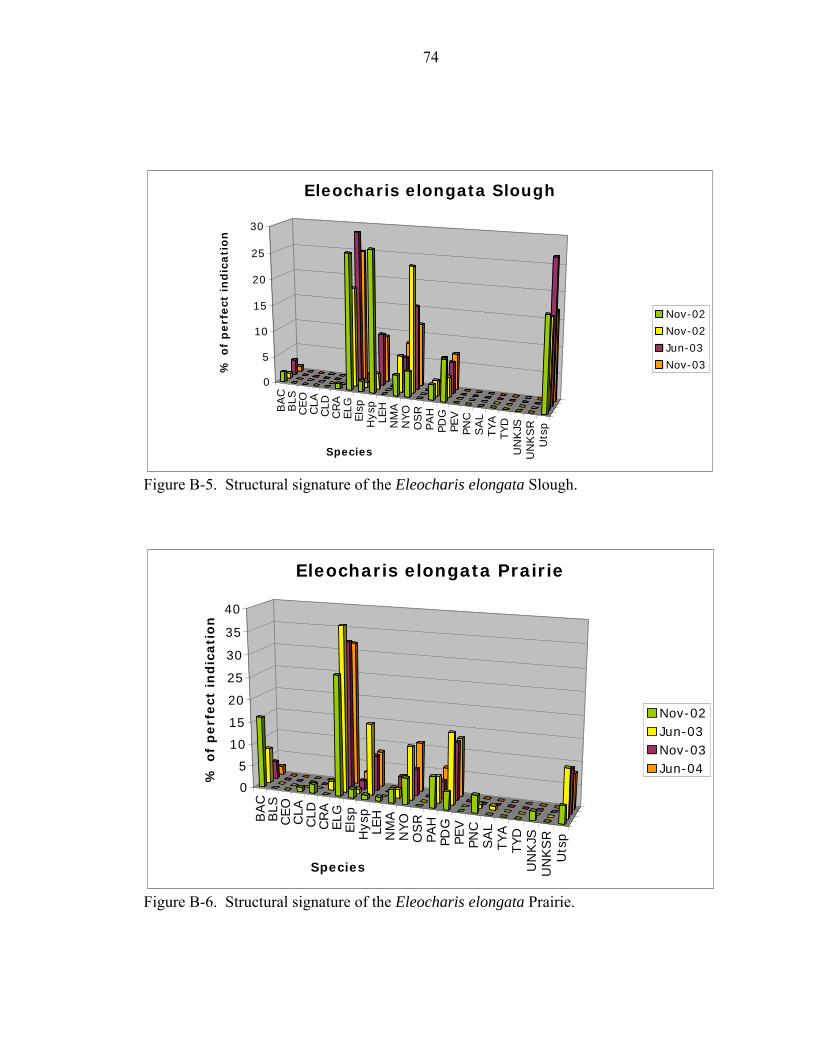
74

BA

CB

LSC

EO

CLA

CLD

CR

AE

LGE

lsp

Hys

pLE

HN

MA

NY

OO

SR

PA

HP

DG

PE

VP

NC

SA

LT

YA

TY

DU

NK

JSU

NK

SR

Uts

p

0

5

10

15

20

25

30%

of

perf

ect

in

dic

ati

on

Species

Eleocharis elongata Slough

Nov-02

Nov-02

Jun-03

Nov-03

Figure B-5. Structural signature of the Eleocharis elongata Slough.

BA

CB

LSC

EO

CLA

CLD

CR

AE

LGE

lsp

Hys

pLE

HN

MA

NY

OO

SR

PA

HP

DG

PE

VPN

CS

AL

TY

AT

YD

UN

KJS

UN

KS

RU

tsp

0

5

10

15

20

25

30

35

40

% o

f p

erf

ect

in

dic

ati

on

Species

Eleocharis elongata Prairie

Nov-02Jun-03Nov-03Jun-04

Figure B-6. Structural signature of the Eleocharis elongata Prairie.

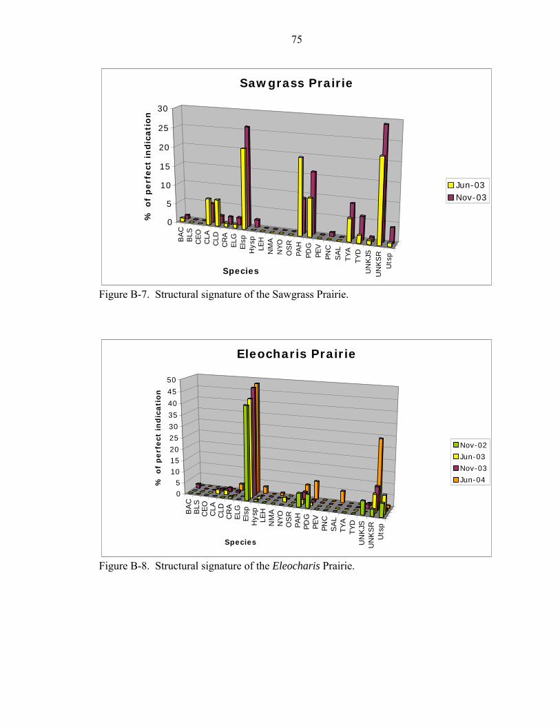
75

BA

CB

LSC

EO

CLA

CLD

CR

AE

LGE

lsp

Hys

pLE

HN

MA

NY

OO

SR

PAH

PD

GP

EV

PN

CS

AL

TY

AT

YD

UN

KJS

UN

KS

RU

tsp

0

5

10

15

20

25

30

% o

f p

erf

ect

in

dic

ati

on

Species

Sawgrass Prairie

Jun-03Nov-03

Figure B-7. Structural signature of the Sawgrass Prairie.

BA

CB

LSC

EO

CLA

CLD

CR

AE

LGE

lsp

Hys

pLE

HN

MA

NY

OO

SR

PA

HP

DG

PE

VP

NC

SA

LT

YA

TY

DU

NK

JSU

NK

SR

Uts

p

05

101520

25

30

35

40

45

50

% o

f p

erf

ect

in

dic

ati

on

Species

Eleocharis Prairie

Nov-02

Jun-03

Nov-03

Jun-04

Figure B-8. Structural signature of the Eleocharis Prairie.

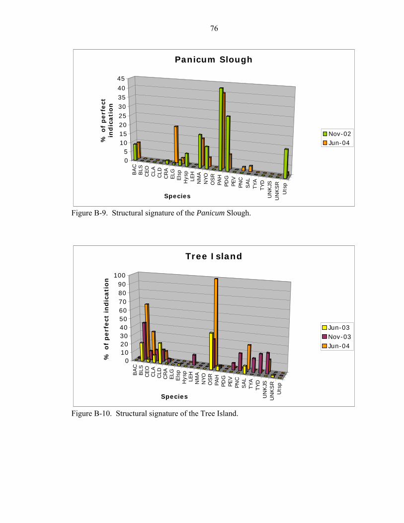
76

BA

CB

LSC

EO

CLA

CLD

CR

AE

LGE

lsp

Hys

pLE

HN

MA

NY

OO

SR

PA

HPD

GP

EV

PNC

SA

LT

YA

TY

DU

NK

JSU

NK

SR

Uts

p

05

10152025303540

45

% o

f p

erf

ect

in

dic

ati

on

Species

Panicum Slough

Nov-02Jun-04

Figure B-9. Structural signature of the Panicum Slough.

BA

CB

LSC

EO

CLA

CLD

CR

AE

LGE

lsp

Hys

pLE

HN

MA

NY

OO

SR

PA

HP

DG

PE

VP

NC

SA

LT

YA

TY

DU

NK

JSU

NK

SR

Uts

p

0102030405060708090

100

% o

f p

erf

ect

in

dic

ati

on

Species

Tree Island

Jun-03Nov-03Jun-04

Figure B-10. Structural signature of the Tree Island.

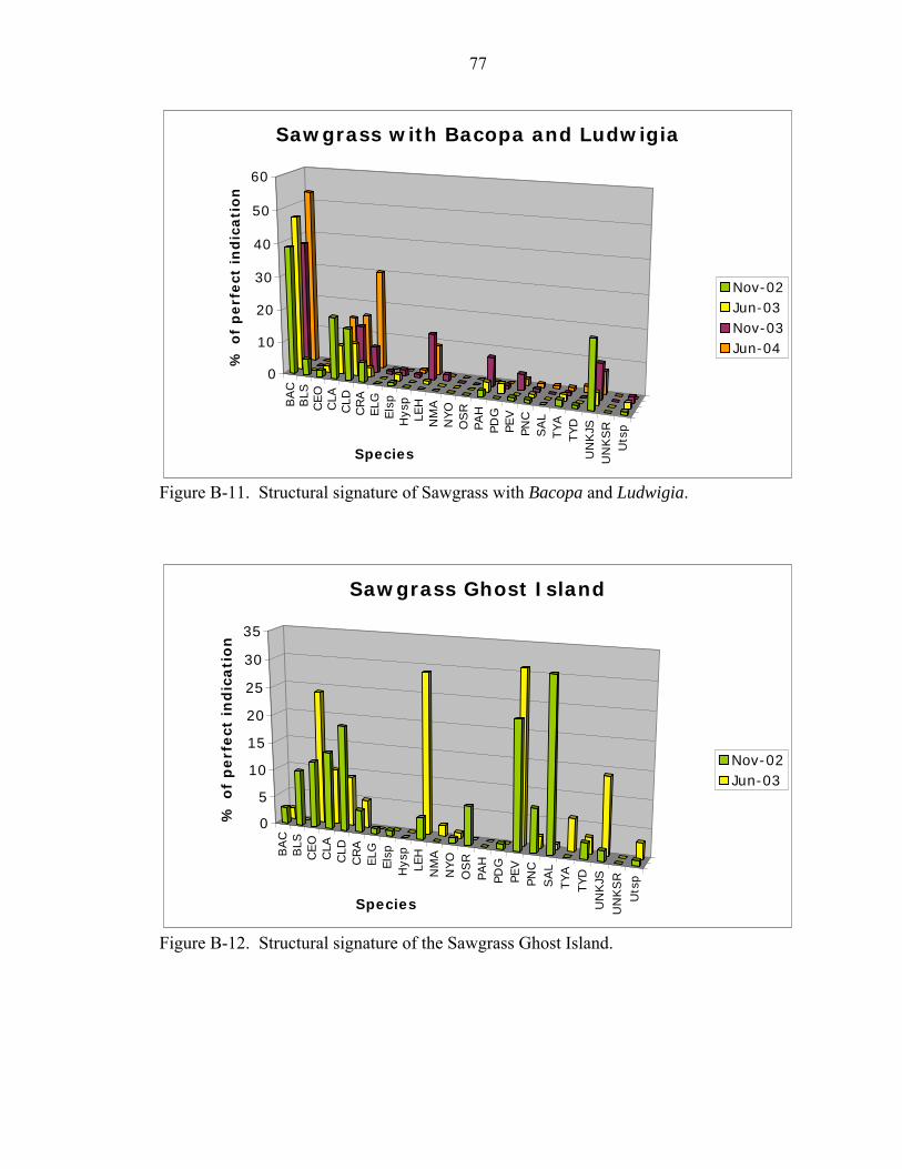
77

BA

CB

LSC

EO

CLA

CLD

CR

AE

LGE

lsp

Hys

pLE

HN

MA

NY

OO

SR

PA

HP

DG

PE

VP

NC

SA

LT

YA

TY

DU

NK

JSU

NK

SR

Uts

p

0

10

20

30

40

50

60

% o

f p

erf

ect

in

dic

ati

on

Species

Sawgrass with Bacopa and Ludwigia

Nov-02Jun-03Nov-03Jun-04

Figure B-11. Structural signature of Sawgrass with Bacopa and Ludwigia.

BA

CB

LSC

EO

CLA

CLD

CR

AE

LGE

lsp

Hys

pLE

HN

MA

NY

OO

SR

PAH

PDG

PEV

PNC

SA

LT

YA

TY

DU

NK

JSU

NK

SR

Uts

p

0

5

10

15

20

25

30

35

% o

f p

erf

ect

in

dic

ati

on

Species

Sawgrass Ghost Island

Nov-02Jun-03

Figure B-12. Structural signature of the Sawgrass Ghost Island.

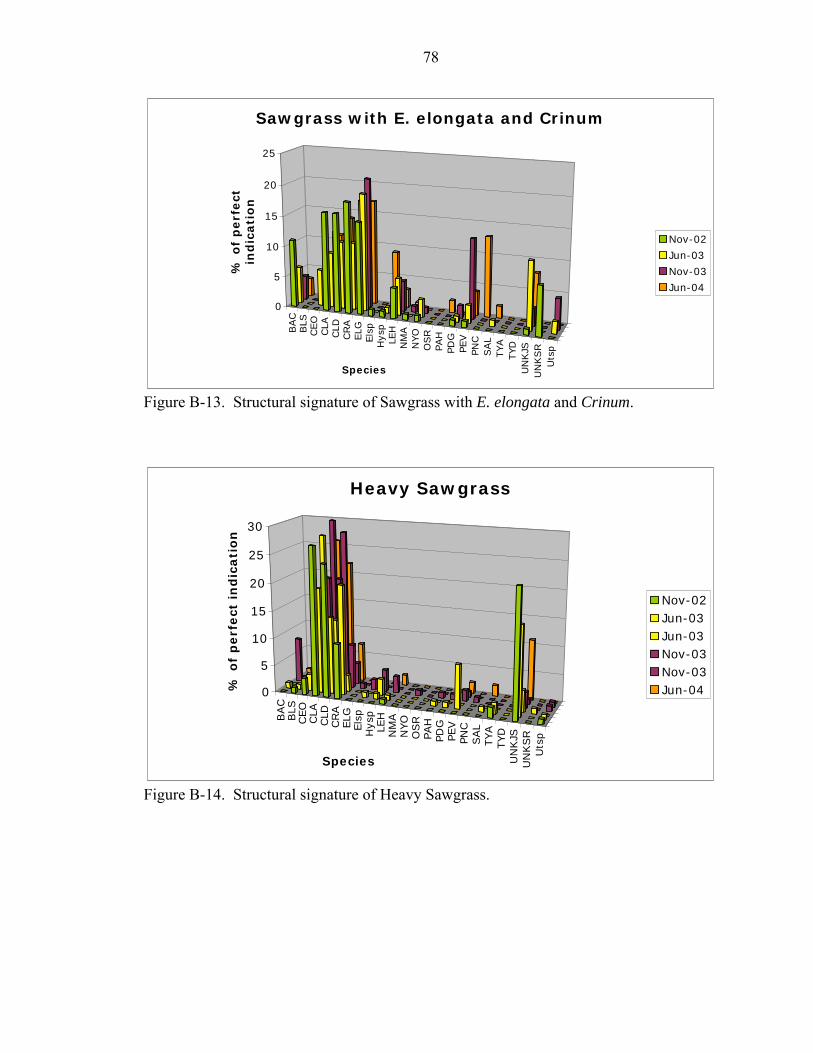
78

BA

CB

LSC

EO

CLA

CLD

CR

AE

LGE

lsp

Hys

pLE

HN

MA

NY

OO

SR

PA

HPD

GP

EV

PNC

SA

LT

YA

TY

DU

NK

JSU

NK

SR

Uts

p

0

5

10

15

20

25

% o

f p

erf

ect

in

dic

ati

on

Species

Sawgrass with E. elongata and Crinum

Nov-02

Jun-03

Nov-03

Jun-04

Figure B-13. Structural signature of Sawgrass with E. elongata and Crinum.

BA

CB

LSC

EO

CLA

CLD

CR

AE

LGE

lsp

Hys

pLE

HN

MA

NY

OO

SR

PA

HPD

GP

EV

PNC

SA

LT

YA

TY

DU

NK

JSU

NK

SR

Uts

p

0

5

10

15

20

25

30

% o

f p

erf

ect

in

dic

ati

on

Species

Heavy Sawgrass

Nov-02Jun-03Jun-03Nov-03Nov-03Jun-04

Figure B-14. Structural signature of Heavy Sawgrass.

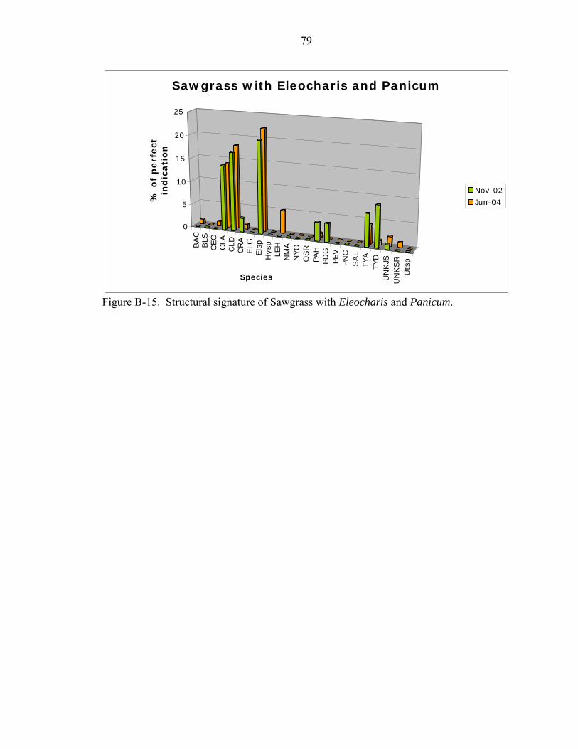
79

BA

CB

LSC

EO

CLA

CLD

CR

AE

LGE

lsp

Hys

pLE

HN

MA

NY

OO

SR

PAH

PDG

PEV

PNC

SA

LT

YA

TY

DU

NK

JSU

NK

SR

Uts

p

0

5

10

15

20

25

% o

f p

erf

ect

in

dic

ati

on

Species

Sawgrass with Eleocharis and Panicum

Nov-02

Jun-04

Figure B-15. Structural signature of Sawgrass with Eleocharis and Panicum.

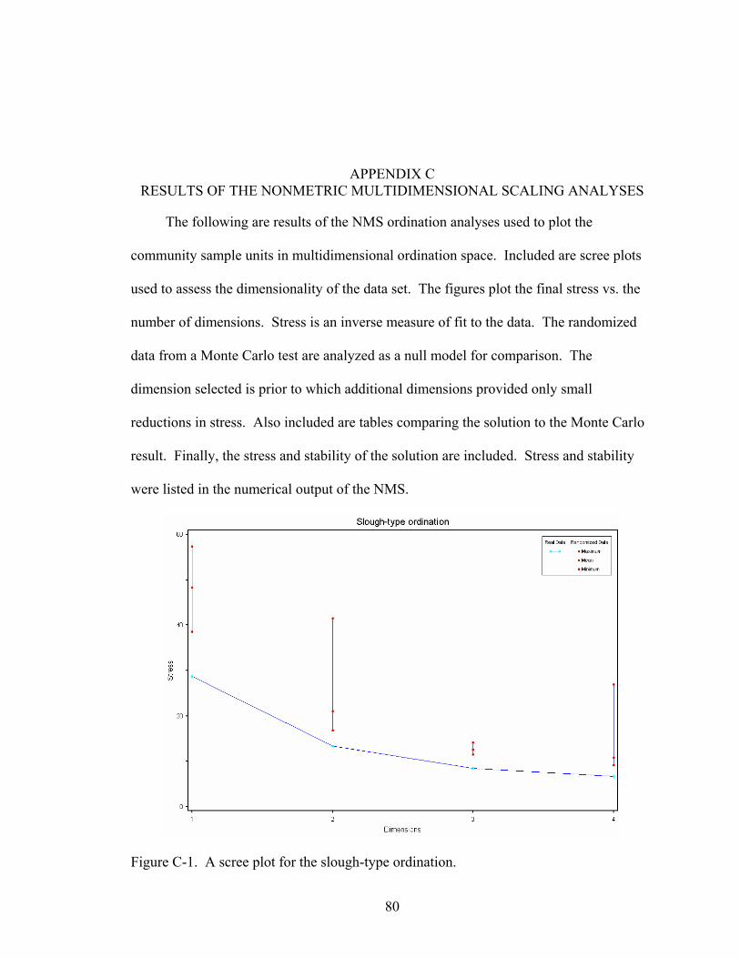
80

APPENDIX C RESULTS OF THE NONMETRIC MULTIDIMENSIONAL SCALING ANALYSES

The following are results of the NMS ordination analyses used to plot the

community sample units in multidimensional ordination space. Included are scree plots

used to assess the dimensionality of the data set. The figures plot the final stress vs. the

number of dimensions. Stress is an inverse measure of fit to the data. The randomized

data from a Monte Carlo test are analyzed as a null model for comparison. The

dimension selected is prior to which additional dimensions provided only small

reductions in stress. Also included are tables comparing the solution to the Monte Carlo

result. Finally, the stress and stability of the solution are included. Stress and stability

were listed in the numerical output of the NMS.

Figure C-1. A scree plot for the slough-type ordination.

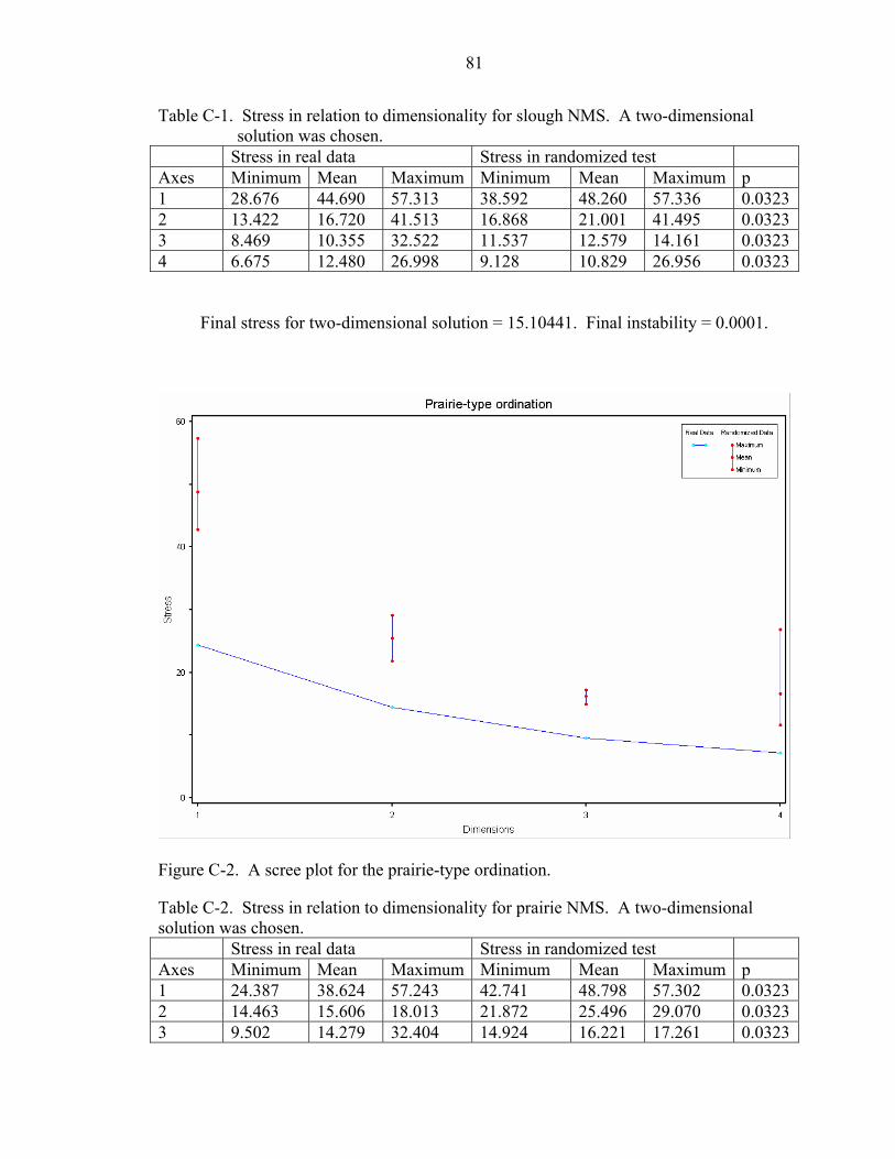
81

Table C-1. Stress in relation to dimensionality for slough NMS. A two-dimensional solution was chosen.

Stress in real data Stress in randomized test Axes Minimum Mean Maximum Minimum Mean Maximum p 1 28.676 44.690 57.313 38.592 48.260 57.336 0.03232 13.422 16.720 41.513 16.868 21.001 41.495 0.03233 8.469 10.355 32.522 11.537 12.579 14.161 0.03234 6.675 12.480 26.998 9.128 10.829 26.956 0.0323

Final stress for two-dimensional solution = 15.10441. Final instability = 0.0001.

Figure C-2. A scree plot for the prairie-type ordination.

Table C-2. Stress in relation to dimensionality for prairie NMS. A two-dimensional solution was chosen. Stress in real data Stress in randomized test Axes Minimum Mean Maximum Minimum Mean Maximum p 1 24.387 38.624 57.243 42.741 48.798 57.302 0.03232 14.463 15.606 18.013 21.872 25.496 29.070 0.03233 9.502 14.279 32.404 14.924 16.221 17.261 0.0323

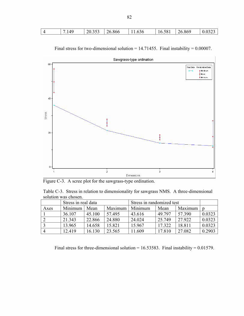
82

4 7.149 20.353 26.866 11.636 16.581 26.869 0.0323

Final stress for two-dimensional solution = 14.71455. Final instability = 0.00007.

Figure C-3. A scree plot for the sawgrass-type ordination.

Table C-3. Stress in relation to dimensionality for sawgrass NMS. A three-dimensional solution was chosen. Stress in real data Stress in randomized test Axes Minimum Mean Maximum Minimum Mean Maximum p 1 36.107 45.100 57.495 43.616 49.797 57.390 0.03232 21.343 22.866 24.880 24.024 25.749 27.922 0.03233 13.965 14.658 15.821 15.967 17.322 18.811 0.03234 12.419 16.130 23.565 11.609 17.810 27.082 0.2903

Final stress for three-dimensional solution = 16.53583. Final instability = 0.01579.

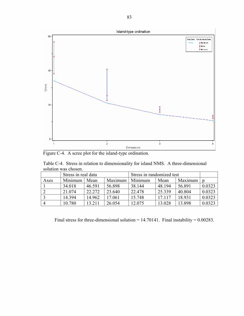
83

Figure C-4. A scree plot for the island-type ordination.

Table C-4. Stress in relation to dimensionality for island NMS. A three-dimensional solution was chosen. Stress in real data Stress in randomized test Axes Minimum Mean Maximum Minimum Mean Maximum p 1 34.018 46.591 56.898 38.144 48.194 56.891 0.03232 21.074 22.272 23.640 22.478 25.339 40.804 0.03233 14.394 14.962 17.061 15.748 17.117 18.931 0.03234 10.780 13.211 26.054 12.075 13.028 13.898 0.0323

Final stress for three-dimensional solution = 14.70141. Final instability = 0.00283.

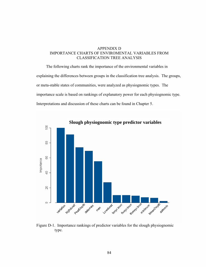
84

APPENDIX D IMPORTANCE CHARTS OF ENVIROMENTAL VARIABLES FROM

CLASSIFICATION TREE ANALYSIS

The following charts rank the importance of the environmental variables in

explaining the differences between groups in the classification tree analysis. The groups,

or meta-stable states of communities, were analyzed as physiognomic types. The

importance scale is based on rankings of explanatory power for each physiognomic type.

Interpretations and discussion of these charts can be found in Chapter 5.

Figure D-1. Importance rankings of predictor variables for the slough physiognomic

type.

Slough physiognomic type predictor variables

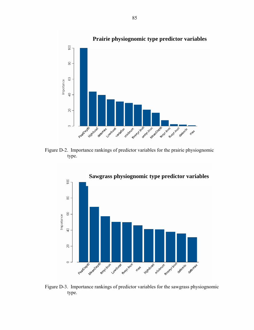
85

Figure D-2. Importance rankings of predictor variables for the prairie physiognomic

type.

Figure D-3. Importance rankings of predictor variables for the sawgrass physiognomic

type.

Prairie physiognomic type predictor variables

Sawgrass physiognomic type predictor variables

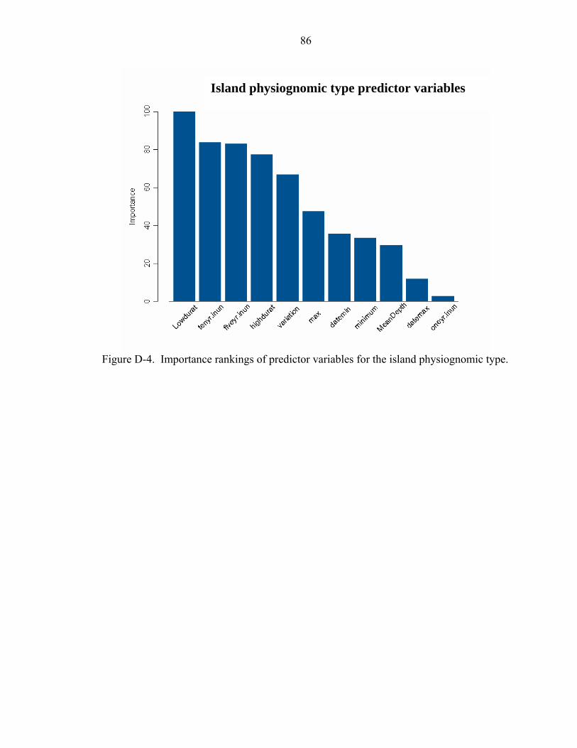
86

Figure D-4. Importance rankings of predictor variables for the island physiognomic type.

Island physiognomic type predictor variables

87

LIST OF REFERENCES

Biondini M, Bonham C, Redente E, 1985, Secondary successional patterns in a sagebrush (Artemisia tridentata) community as they relate to soil disturbance and soil biological activity. Vegetatio 60:25-36.

Bishop C, 1995, Neural Network for Pattern Recognition. Oxford University Press, New York City, New York.

Carpenter S, Walker B, Anderies J, Abel N, 2001, From metaphor to measurement: resilience of what to what? Ecosystems 4:765-781.

Clarke K, and Ainsworth M, 1993, A method of linking multivariate community structure to environmental variables. Marine Ecology Progress Series 92:205-219.

Davis J, 1943, The natural features of southern Florida. Fla. Geol. Surv. Biol. Bull. No. 25. Tallahassee, FL, USA.

Davis S, Gunderson L, Park W, Richardson J, Mattson J, 1994, Landscape dimension, composition, and function in a changing Everglades ecosystem. In Everglades: The Ecosystem and Its Restoration, Davis S and Ogden J (Eds.), St. Lucie Press, Delray Beach, FL, pp. 419-444.

DeAngelis D, 1994, Synthesis: Spatial and temporal characteristics of the environment. In Everglades: The Ecosystem and Its Restoration, Davis S and Ogden J (Eds.), St. Lucie Press, Delray Beach, FL, pp. 307-321.

DeAngelis D, and White P, 1994, Ecosystems as products of spatially and temporarily varying driving forces, ecological processes, and landscapes: a theoretical perspective. In Everglades: The Ecosystem and Its Restoration, Davis S and Ogden J (Eds.), St. Lucie Press, Delray Beach, FL, pp. 9-28.

Dufrene M, and Legendre P, 1997, Species assemblages and indicator species: the need for a flexible asymmetrical approach. Ecological Monographs 61:53-73.

Gerritsen J, and Greening H, 1989. Marsh seed banks of the Okefenokee swamp: effects of hydrologic regime and nutrients. Ecology 70:750–763.

Gleason P, and Stone P, 1994, Age, origin, and landscape evolution of the Everglades peatland. In Everglades: The Ecosystem and Its Restoration, Davis S and Ogden J (Eds.), St. Lucie Press, Delray Beach, FL, pp. 149-198.

88

Gunderson L, and Pritchard L, 2002, Resilience and the Behavior of Large Scale Ecosystems. SCOPE volume, Island Press, Washington, DC.

Gunderson L, 1994, Vegetation of the Everglades: determinants of community composition. In Everglades: The Ecosystem and Its Restoration, Davis S and Ogden J (Eds.), St. Lucie Press, Delray Beach, FL, pp. 323-340.

Gunderson L, Loftus W, 1993, The Everglades: competing land uses imperil the biotic communities of a vast wetland. In Biotic Communities of the Southeastern United States, Martin W, Boyce S, and Esternacht A (Eds.), John Wiley and Sons, New York, NY, pp. 123-134.

Herndon A, Gunderson L, Stenberg J, 1991, Sawgrass (Cladium jamaicense) survival in a regime of fire and flooding. Wetlands 11:17-27.

Holling C, 1973, Resilience and stability of ecological systems. Annual Review of Ecology and Systematics 4:1-24.

Jordan F, Babbitt K, McIvor C, Miller S, 1996, Spatial ecology of the crayfish Procambarus alleni in a Florida wetland mosaic. Wetlands 16:134-142.

Jordan F, Jelks H, Kitchens W, 1994, Habitat use by the fishing spider Dolomedes triton in a northern Everglades wetland. Wetlands 14:239-242.

Kent M, and Coker P, 1992, Vegetation Description and Analysis: A Practical Approach. CRC Press Inc., Boca Raton, FL.

Kitchens W, Bennetts R, DeAngelis D, 2002, Linkages between the snail kite population and wetland dynamics in a highly fragmented South Florida landscape. In The Everglades, Florida Bay, and Coral Reefs of the Florida Keys: An Ecosystem Sourcebook, Porter J and Porter K (Eds.), CRC Press, Boca Raton, FL, chapter 6.

Kruskal J, 1964, Nonmetric multidimensional scaling: a numerical method. Psychometrika 29:115-129.

Loftus W, Kushlan J, 1987, Freshwater fishes of southern Florida. Bulletin of the Florida State Museum, Biological Sciences 31:147-344.

Loveless C, 1959, A study of the vegetation in the Florida Everglades. Ecology 40:1-9.

Mather P, 1976, Computational methods of multivariate analysis in physical geography. J. Wiley & Sons, London.

McCune B, and Grace J, 2002, Analysis of Ecological Communities. MJM Software Design, Gleneden Beach, OR.

McPherson B, 1973, Vegetation in Relation to Water Depth in Conservation Area 3, Florida. U.S. Geological Survey Open-File Report No. 73025, Tallahassee, FL.

89

Richter B, Baumgartner J, Wigington R, Braun D, 1997, How much water does a river need? Freshwater Biology 37:231-249.

Richter B, Baumgartner J, Powell J, Braun D, 1996, A method for assessing hydrologic alteration within ecosystems. Conservation Biology 10:1163-1174.

Scheffer M, Carpenter S, Foley J, Folke C, Walker B, 2001, Catastrophic shifts in ecosystems. Nature 413:591-596.

Smith S, McCormick P, Leeds J, Garrett P, 2002, Constraints of seed banks and water depth for restoring vegetation in the Florida Everglades, U.S.A. Restoration Ecology 10:138-145.

Toner M, and Keddy P, 1997, River hydrology and riparian wetlands: a predictive model for ecological assembly. Ecological Applications 7:236-246.

Urban D, 2002, Classification and regression trees. In Analysis of Ecological Communities. MJM Software Design, Gleneden Beach, OR, pp. 222-232.

van der Valk A, 1991, Response of wetland vegetation to a change in water level. In Wetland Management and Restoration, C Finlayson and T Larson (Eds.), Proc. Workshop, Solna, Sweden 1990, Swedish Environmental Protection Agency Report, pp. 7-15.

Weisner S, and Miao S, 2004, Use of morphological variability in Cladium jamaicense and Typha domingensis to understand vegetation changes in an Everglades marsh. Aquatic Botany 78:318-335.

Weisner S, and Strand J, 1996, Rhizome architecture in Phragmites australis in relation to water depth: implications for within-plant oxygen transport distances. Folia Geobot. Phytotax 31:91–97.

White P, 1994, Synthesis: Vegetation pattern and process in the Everglades ecosystem. In Everglades: The Ecosystem and Its Restoration, S Davis and J Ogden (Eds.), St Lucie Press, Delray Beach, FL, chapter 18.

Wishart D, 1969, An algorithm for hierarchical classifications. Biometrics 25:165-170.

Wood J, and Tanner G, 1990, Graminoid community composition and structure within four Everglades management areas. Wetlands 10:127-149.

Wunderlin R, 1998, Guide to the Vascular Plants of Florida. University Press of Florida, Gainesville.

90

BIOGRAPHICAL SKETCH

Erik Norman Powers was born in Corpus Christi, Texas, on September 2, 1976. He

grew up in Destin, Florida, after having resided briefly outside Mobile, Alabama. From

1994-1996 he attended the Oregon Institute of Technology. He transferred to the

University of Florida in 1997 and received a Bachelor of Science degree in

environmental science. Following a two-year employment stint at C&N Environmental

Consulting, Inc., he began the graduate program at the University of Florida through the

School of Natural Resources under Wiley Kitchens. He married Kristy Shreve on August

21, 2004, in Destin. Kristy and Erik are expecting their first child in March 2006.