Measuring (in a time of crisis) the impact of broadband ... · Sezione di Statistica Economica ed Econometria Angelo Castaldo Alessandro Fiorini Bernardo Maggi Measuring (in a time

Dipartimento di Scienze Statistiche

Sezione di Statistica Economica ed Econometria

Angelo Castaldo Alessandro Fiorini

Bernardo Maggi

Measuring (in a time of crisis) the impact ofbroadband connections on economic

growth: an OECD panel analysis

DSS Empirical Economics and EconometricsWorking Papers Series

DSS-E3 WP 2016/1

Dipartimento di Scienze StatisticheSezione di Statistica Economica ed Econometria

“Sapienza” Università di RomaP.le A. Moro 5 – 00185 Roma - Italia

http://www.dss.uniroma1.it

1

Measuring (in a time of crisis) the impact of broadband connections

on economic growth: an OECD panel analysis

Angelo Castaldo Alessandro Fiorini

Bernardo Maggi

Abstract: Technological innovation is viewed as a major stimulus for economic growth. High-speed internet access via

broadband infrastructure has been experiencing a prompt development since the end of 90s, thanks to the deployment

of both fix and mobile technologies. The present study investigates on the behavior of broadband diffusion as a

technological determinant of economic growth in the main OECD countries. The estimations performed allowed to

control and interpret the time evolution of the phenomenon according to the achievable target of growth, as resulting

from the promotion of broadband internet connections. Our main goal is to provide evidence of a relevant - in

quantitative term - relation between broadband diffusion and economic dynamics in the short, medium and long run.

Key words: Broadband access, economic growth, technology diffusion, logistic curve, dynamic

panel

JEL classification: L96, O47, O33, H54

1. Introduction Why should countries facilitate the deployment of broadband (BB) and ultra wideband (UWB) communication networks? Information and Communication Technologies’ (ICT) networks are commonly recognized as crucial drivers for economic and social development. Serving as communication and transaction platforms they represent, since their origin, a key component for both creation and diffusion of knowledge through which individuals, firms and governments can interact in a more efficient way (von Hayek, 1945). Given the high positive spillovers, ICT infrastructures can determine structural changes in an economic system mainly supporting factor’s productivity growth across all sectors (Katz et al. 2010; Greenstein and McDevitt, 2011; Stryszowski, 2012). There is a widespread belief that internet diffusion leads to a significant impact on socio-economic variables. Internet, in particular, rose up as a facility devoted to the improvement of communication systems but has soon turned into a ubiquitous technology supporting all sectors across the economy (Oz, 2005; Flamm and Chaudhuri, 2007). Internet, therefore, is now widely considered as an essential platform, besides electricity, water and transportation networks and can now be considered as a ‘general purpose technology’ (Holt and Jamison, 2009; Majumdar et al., 2009). In this field of research, as a consequence of the rapid technological innovations achieved, the debate during the last twenty years has naturally shifted on broadband (BB) internet access. Advanced communication networks are a key component of innovative ecosystems and strongly support economic growth (Czernich et al., 2011; Koutroumpis, 2009; Qiang et al. 2009; Crandall et al., 2007; Datta and Argawal, 2004; Roller and Waverman, 2001). Broadband networks also increase the impact and efficiency of public and private investments that depend on high-speed communications. Broadband is seen as a complementary investment linked to other infrastructures such as buildings, roads, transportation systems, health and electricity grids, allowing them to be “smart” and save energy, assist the aging, improve safety and adapt to new ideas (OECD, 2009).

Corresponding author and Sapienza University of Rome, Department of Law, Philosophy and Economic Studies, Faculty of Law, P.le

Aldo Moro 5, 00185, Rome, Italy. Sapienza University of Rome, Department of Law, Philosophy and Economic Studies, Faculty of Law, P.le Aldo Moro 5, 00185, Rome,

Italy Sapienza University of Rome, Department of Statistical Sciences, Faculty of Engineering of Information, Informatics and Statistics, P.le

Aldo Moro 5, 00185, Rome, Italy.

2

The term broadband (BB), however, entails a number of complex issues in terms of technologies, speeds and quality of services (ITU, 2011). Broadband is commonly used to define a form of high speed access to communication technologies. International Telecommunication Union (ITU) fixes at 256 kbit/s the lower bound to recognize a broadband internet connection, including alternative technologies such as cable modem, Digital Subscribers Line (xDSL) and fiber, in case of portable internet; satellite subscriptions, terrestrial fixed wireless subscriptions and terrestrial mobile wireless subscriptions in case of mobile broadband connections. The Organization of Economic Cooperation and Development (OECD) assumes 256 kbit/s in at least one direction. Even though the bit rate set by ITU and OECD is the baseline for the most national institutions’ standards, broadband definition seems to be an open issue1. Setting a minimum level based on speed of connection for the definition of broadband is certainly a complicated task, because both technologies and services/applications evolve; this leads to a difficult comparability among similar variables over time. Socio-economic structural reforms seem to be a key policy factor in order to bank the effects of the severe economic downturn suffered by Nations from 2008 (e.g. Horizon 2020 - European Digital Agenda for UE and Competes Act (PL 110-69) for US). The significant penetration and improvement of ICT broadband (BB) facilities can certainly play a leading role in conjugating innovation in terms of productivity gains, thus strategies adopted by policy makers for setting up recovery patterns should be viewed as opportunities for targeting investment in strategic areas such as broadband (OECD, 2009)2. This paper provides a contribution to the measurement of the impact of broadband penetration (fixed internet connections equal or faster than 256 kbit/s) on growth. More specifically, our goals and advancements in the literature are: a) to model in a proper dynamic way the impact of broadband penetration (BB) on GDP per capita, in order to deal appropriately with broadband spillovers over time b) to test if the geographical endowment of ICT innovation capacity interacts with broadband penetration deployment; c) to test the if the beneficial effect on growth due to broadband is still relevant during an economic downturn; d) to forecast the impact of broadband on GDP per capita in the short, medium and long run for each country of our panel; e) assimilated the lesson learned from BB impact on growth in the transition from copper to partially fiber networks, to foresee the impact on growth that could be driven by a new technology shift, i.e., the full deployment of new upgraded ultra wideband (UWB) networks.3 The paper is organized as follows. In Section 2 a review of the main literature concerning broadband/ICT technologies and economic growth is presented. Section 3 and 4 describe models’ equations, data and variables used. In section 5 econometric methodology adopted is described. Section 6 presents the estimations results. Section 7 shows the main policy implications. Finally, Section 8, draws the conclusions. 2. Literature survey Our work is placed in the endogenous set up of growth models with externalities pioneered by Lucas (1988), Romer (1990) and Barro (1991). Other seminal contributions funded on a technologically endogenous growth model, elaborated by Mankiw et al. (1992) and Aghion and Howitt (1992), generated a consistent field of research based on an equilibrium approach appositely specified in order to study the relationship between broadband penetration and GDP. The impacts of broadband infrastructures on economic growth have been discussed in a large number of works. Overall results support the view that broadband access enhances economic growth and that causality impacts are real and measurable. Several studies, however, have been considered biased due to common time trends, omitted variables, simultaneity and reverse causality.

1 For example, the US Federal Communication Commission (FCC) identifies a broadband connection as “transmission service […] enables an end user to download content from the Internet at 4 Mbps and to upload such content at 1 Mbps over the broadband provider’s network”. In Djibuti and Morocco, so as in other developing countries, the bit rate is set at 128 kbit/s (ITU, 2011). 2 As remarkable example Korea and Finland experienced high positive returns as leading countries in the diffusion of broadband technologies (Kim et al., 2010). 3 Communication infrastructures and technology able to carry out services at a speed of at least 30 Mbit/s in download and at least of 3 Mbit/s in upload.

3

Roller and Waverman (2001) investigated on growth across 21 OECD countries from 1970 to 1990 and showed that almost one third of the per capita GDP growth (0.59 of the 1.96 percent per year growth rate) was to be attributed to investments in telecommunications infrastructures. Moreover, the study gives evidence of important fixed effects and of reverse causality issues. Datta and Agarwal (2004) empirically evaluate, in a sample of 22 OECD countries, the impact of telecommunication infrastructure (access lines per 100 inhabitants) on economic growth. The authors implement a panel data model with a dynamic fixed-effect method estimation technique; fixed effects are specified in order to deal with country specific differences in aggregate production functions. The results show that telecommunications infrastructures are statistically significant and highly positively correlated with growth in GDP per capita; moreover, results are robust after accounting for investment, government consumption, population growth, openness, past levels of GDP and lagged growth. Gillet et al. (2006) found that the availability of broadband connections may explain relevant gaps in growth and employment. In particular, the approach followed uses a panel data set in order to catch the effects of broadband on communities in the US between 1998 and 2002. Crandall et al. (2007) found a strong association between broadband (BB) adoption and economic prosperity in United States of America, through the channel of job creation and GDP. During the period 2003-2005, they estimate that a 1% increase in BB penetration, produced an increase in the annual rate of employment, in industrial sectors, from 0.2 up to 0.3 percentage points, as regards the effects of BB deployment on GDP. Holt and Jamison (2009), in surveying the main studies on BB and GDP in the case of United States of America, observe a positive impact on GDP of BB but considers the impact not precise. In the opinion of the authors, the uncertainty on the impact are mainly due to two reasons: a) impacts evolve in time with nonlinearities, even going through periods of negative growth and b) endogeneity can affect workforce change, broadband adoption and, more generally, other determinants. Cznernich et al. (2011) cope with such questions by better identifying the penetration rate with the use of a logistic function based on available physical infrastructure. They estimate the effect of broadband infrastructure on economic growth relying on a panel dataset of OECD countries in 1996–2007. Their aim is to estimate a long run equilibrium à la Mankiw et al. (1992) by means of a first difference approach. Other similar works that seek to study an equilibrium relationship are, among others, Bresnahn et al. (2002), Bloom and Van Reenen (2007) and Cappelli (2010). From the cited literature, however, there are still some relevant open questions that need to be addressed. First, empirical studies that implement an equilibrium approach miss the adjustment phase both in the study of the time pattern of growth and in the attainability of the equilibrium itself. Second, equilibrium (long run) relationships require specific empirical treatment (Breitung and Pesaran, 2008) to be accurately tested on long time series that are not usually available for the dataset used by the literature till now; in particular, neither suffices to this aim a first difference approach. Finally, endogeneity issues are only partially addressed.

3. Model equations and strategy of analysis

As said, in the present context traditional growth models derive from a dynamic set up but are confined to the analysis of the steady state without focusing on the transitional dynamics. This is the case of the Mankiw et al. (1992) set up and of the subsequent stream of works cited in the previous section. In the shade of such a framework, our approach, even though grounded on the above mentioned Mankiw model, focuses on the dynamic pattern of the phenomena and derives the equilibrium relationship moving from an adjustment process. Further, we conceive the broadband penetration as playing a crucial role inside the technological component and extend the equilibrium relation in order to examine the incidence of the recent economic crisis. The output steady state relation we intend to test is therefore

(1) ss

it t l it hk it k ity a l hk s , i =1,….,N; t=1,….., T

4

with the technical progress

(2) 0 _ , _ , _ , ,b

t BB it i i i ita F MOB NET TEL NET CAB NET t Θ

The third equation of our model defines the adjustment of the actual output to its steady state relation

(3) 0 1_ , _ , _ , ,c

b

it BB it i i i LF l it hk it k it D c it ity F MOB NET TEL NET CAB NET t LF l hk s D y Θ

which is equivalent to the lagged equation (3’) 1 01 .

c

b

it it BB it LF l it hk it k it D c ity y F LF l hk s D

symbols in lower and capital case characters indicate that variables are in natural logarithms and in natural numbers, respectively, i and t are countries and time. Eq. (1) defines the steady state and considers the steady state output per worker (yss), technical progress (a), workforce (l), human capital (hk), investments (s). In eq. (2), as said above, Fb(.) models the broadband penetration as a function that accounts for the relevance of initial existing communication infrastructures - i.e., fixed network (TEL_NET), mobile network (MOB_NET) and cable (CAB_NET)- on the actual broadband

penetration pattern and is a parameters vector to be estimated. This step of the analysis, in accounting for the initial endowment of communication infrastructures, helps make clear to which extent broadband deployment (adsl/vdsl and fiber) is influenced by previous and more traditional communication services level of diffusion (copper, cable and GSM). Thus, this instrumental stage (IV) is conducted in order to control for the main initial conditions that explain diffusion (from the very beginning to the mature stage) of the new technology (BB), in terms of transition from traditional to next generation networks. Thus, Fb(.) is the function that represents the broadband penetration, BB, given by the percentage of broadband subscribers over 100 inhabitants (connections with downstream speeds equal or greater to 256 kbit/s). Equation (3), finally, defines the equation we intend to estimate according to an Equilibrium Adjustment Model approach (EAM). This is in line with Islam (1995), and

allows capturing short run autoregressive behavior of the dependent variable by means of , which is

the speed of adjustment, and =1/, which is the mean time lag. Moreover, in equations (3) and (3’), in order to further qualify such an adjustment in disequilibrium, we also introduce two dummy variables, Dc and LF, which refer to the years of economic financial crisis and to countries in position of leader or follower in the ICT innovation capacity, respectively. However, in order to let a comparison with the above cited literature based on the Mankiw model, we estimate equation (1) also using an Equilibrium Model approach (EM) a là Cznernich et al., (2011) and adopt the following equation (4):

(4) 2

1 1 0

B

it BB it BBt it l it hk it k it t it y i ity BB BB l hk s T y

We underline that the ongoing empirical literature tries to estimate directly the equilibrium relation of eq. (1) by considering the so called “difference in difference” relation (eq. 4) and introducing accessory control variables to disentangle from the data the long run relation. The use of control variables might mitigate the absence of an adjustment process linked to technology here represented by broadband penetration. In Cznernich et al. (2011) these controls are time variables, such as the exogenous years (TB) since the beginning of broadband penetration, and country-specific initial GDP per capita condition (yi0) in order to take into account the out-of-steady-state dynamics and the - neoclassical - convergence hypothesis, respectively. However, from an empirical point of view, the strategy of using first differenced variables does not allow to obtain unequivocally a steady state relation since the estimated relation could be of a long run as well as of short run.

5

Furthermore, the differentiation adopted in the estimation does not seem useful given that the length of the time series does not allow for powerful tests of cointegration and stationarity of the variables. For the same reason it is reductive to confine the endogeneity problem to the broadband penetration rate, while it is to be referred to all the set of variables. We address and solve such points by proposing an EAM approach (eq. 3) which considers the adjustment process towards the equilibrium based on instrumental variables. In such a way we are capable both to test and assess on the nature (equilibrium or short run relation) of the estimated equation and deal with the problem of endogeneity in a consistent way. Moreover, considering an adjustment process allows also to cope with the nonlinear effects determined by broadband penetration on growth due the time adoption for the economic system to bank the spillovers arising from new technologies (Holt and Jamison, 2009). As regards the way of modeling the “profile” of time evolution assumed by broadband diffusion, Fb(.), penetration rate for many OECD countries suggests that the pattern of broadband technologies’ diffusion mimic a ‘S-shaped curve’ as indicated by the theory of diffusion of innovations (Everett; 1995) and technologies (Comin et al.; 2006). Among the several functional expressions through which such a curve may be formalized, the logistic is one of the most employed (Gruber, 2001; Gruber and Verboven, 2001; Comin et al., 2006; Singh, 2008; Lee et al., 2011). Moreover, the effects of network externalities play a leading role as determinants of the diffusion (Gruber and Verboven, 2001). Connections develop as the result of an exponential dynamic. At a certain starting period, the broadband diffusion process concerns few people. As the number of subscribers begins to increase, a larger amount of people will be involved by the valuation of the opportunity to access for interacting with the other users, triggering a further increase in the number of subscribers. Conversely, when the number of users approaches the total number of potential adopters in the market, the rate of growth of new subscribers declines down to zero, leading the number of total subscribers up to a saturation point due to the congestion, or low valuation for broadband services, among the remaining non-subscribers (Lee et al.; 2011). 4. Variables and data

Our panel is composed of 17 years (1996-2012) and 23 OECD countries: Australia, Austria, Belgium,

Canada, South Korea, Denmark, Finland, France, Germany, Japan, Greece, Ireland, Iceland, Italy,

Norway, New Zealand, The Netherlands, United Kingdom, Spain, United States, Sweden, Switzerland,

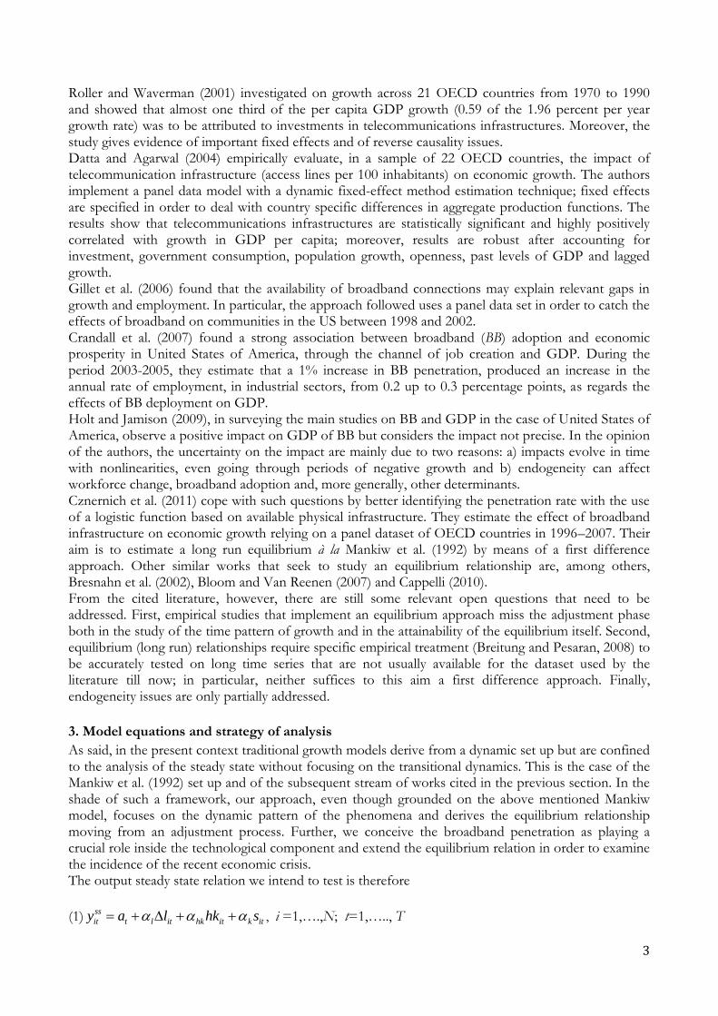
Hungary. Variables are from OECD and ITU database. Table 1 shows the mean and the standard

deviation for the variables used. In Table 1 we specify our variables as follows. GDP is expressed in

thousands per worker (Y) in US dollars, population is in percentage of the broadband subscribers (BB),

HK is the share of population holding a 3rd level education title and working as researcher, i.e. skilled

human capital, ∆L/L is the rate of variation of workforce, S is the ratio between gross fixed capital

formation and GDP. We use GDP in PPP US dollars at 2005 prices for the estimation. As for the

instrumental logistic function, Fb(.), we consider the following independent variables: the subscribers

over 100 persons of mobile networks (MOB_NET), of wired networks (TEL_NET) and of cable

networks (CAB_NET).

Table 1. Descriptive statistics Y BB HK ∆L/L S TEL_NET CAB_NET MOB_NET

Australia

Mean 50.11 14.76 0.96 1.54 25.97 48.80 2.15 31.12

Std.dev. 3.96 9.30 0.14 0.34 1.75 4.41 1.64 31.12

Austria

Mean 48.02 15.05 0.27 0.31 22.59 45.82 15.38 85.40

Std.dev. 3.95 6.70 0.07 0.39 1.36 4.38 3.74 43.17

6

Belgium

Mean 46.86 20.17 0.40 0.47 20.56 46.69 37.50 70.90

Std.dev. 3.09 8.16 0.09 0.34 0.89 2.10 1.01 37.77

Canada

Mean 48.20 20.75 0.59 1.19 20.55 60.72 25.27 42.37

Std.dev. 3.37 7.64 0.08 0.11 1.47 6.07 1.06 20.53

South Korea

Mean 29.36 26.92 0.62 1.64 30.12 51.58 23.55 67.08

Std.dev. 4.89 5.41 0.11 1.07 2.69 4,98 5.99 30.10

Denmark

Mean 48.14 23.40 0.62 0.17 19.16 61.75 27.36 82.23

Std.dev. 2.89 13.22 0.20 0.11 1.28 7.95 6,78 34.91

Finland

Mean 43.22 20.55 0.70 0.27 19.63 44.56 18.48 91.21

Std.dev. 5.14 10.00 0.19 0.12 0.93 11.74 1.56 36.04

France

Mean 45.05 16.33 0.66 0.55 18.89 56.74 5.06 62.06

Std.dev. 2.58 11.72 0.04 0.20 1.26 0.89 0.88 31.65

Germany

Mean 46.25 15.78 0.32 -0.21 19.13 61.05 24.04 74.96

Std.dev. 3.16 11.25 0.09 0.33 1.71 4.59 1.85 43.23

Japan

Mean 43.90 16.56 0.50 -0.51 23.67 45.35 14.63 64.45

Std.dev. 2.91 8.23 0.02 0.30 2.34 6.15 3.30 22.74

Greece

Mean 33.03 6.87 0.18 0.34 21.63 51.56 6.85 72.61

Std.dev. 4.57 7.64 0.20 0.25 2.37 3.97 5.23 39.34

Ireland

Mean 50.46 10.22 0.85 1.76 21.78 47.66 14.16 76.65

Std.dev. 7.26 8.76 0.14 1.05 3.93 3.76 2.07 37.22

Iceland

Mean 47.98 21.70 0.79 1.48 22.18 63.88 1.07 81.09

Std.dev. 4.52 11.44 0.26 1.35 5.57 3.41 0.86 31.18

Italy

Mean 41.05 11.20 0.44 0.12 20.29 43.28 6.42 96.03

Std.dev. 2.00 7.93 0.14 0.42 0.83 4.46 15.20 48.28

Norway

Mean 68.84 20.12 0.67 0.97 20.22 48.33 20.54 83.01

Std.dev. 3.80 13.16 0.07 0.28 2.12 8.07 4.93 28.26

New Zealand

Mean 36.03 11.20 0.87 1.24 21.38 44.62 0.34 66.22

Std.dev. 2.61 9.32 0.10 0.57 1.51 2.53 0.26 35.11

The

Netherlands

Mean 50.37 23.50 0.61 0.36 20.36 50.73 38.52 77.10

Std.dev. 4.03 13.41 0.12 0.18 1.56 6.51 0.72 40.11

United

Kingdom

Mean 47.04 16.41 0.78 0.56 16.69 56.44 8.79 83.81

Std.dev. 3.64 11.84 0.10 0.50 0.82 1.97 7.05 41.55

7

Spain

Mean 37.71 13.28 0.50 1.09 25.97 42.84 2.56 73.99

Std.dev. 3.13 7.41 0.04 0.70 3.12 2.00 2.76 38.38

United States

Mean 60.42 16.44 0.70 1.13 18.39 60.12 23.28 55.72

Std.dev. 3.65 8.41 0.06 0.27 1.59 6.62 0.54 25.86

Sweden

Mean 47.09 20.26 0.51 0.58 17.70 62.89 19.81 84.01

Std.dev. 4.46 10.84 0.08 0.25 1.16 5.33 8.18 29.26

Switzerland

Mean 51.83 21.46 0.43 0.77 21.68 68.05 36.61 76.18

Std.dev. 2.53 13.02 0.09 0.36 0.98 5.09 1.36 38.20

Hungary

Mean 22.21 9.38 0.58 -0.12 22.26 33.16 15.67 67.37

Std.dev. 3.04 7.21 0.07 0.09 1.54 3.24 6.90 44.30

Given the importance of the dynamic catching up pattern between BB and GDP, in order to test the

relevance of technological ICT endowment for each country, we structured a leader-follower (LF)

dummy variable according to ITU – ICT Development Index (IDI). We assume as leaders the U.S.,

South Korea, Denmark, Finland, France, Japan, Iceland, Norway, Netherlands and Sweden by being

above the mean of IDI index value.

Moreover, given the specific GDP fluctuations registered in the years of economic crisis, we tested the

existence of a structural break during (2007-2008-2009)4 by introducing a ‘crisis’ dummy variable (Dc).

5. Econometric methodology, EAM approach

Given the exigency of treating appropriately the dynamics and the simultaneity problems discussed in Section 3, our straightforward method to implement the EAM approach, is the Arellano-Bond dynamic panel GMM estimator with one lag applied to equation (3’), which in this case displays as:

the estimation equation

(7) 1 1tZ Y Z Y Z X Z

where vectors and matrices refer to variables stacked by space and time;

Among itX the strictly (i.e., lagged) predetermined (k1=4) and exogenous (k2=2, i.e., LF, j)

regressors5 are used to obtain the necessary instruments ( iZ )

(8) (.), , , , , ,b

it it it it it itX f s hk l y lf j , 0it isE X with t ≥ s, and Xit ≠ t, j, j =1,.........,1;

the parameters vector is

(9) 0, , , , , ,cl hk k d BB lf ;

the errors term structure is

(10) MA(1), 1,.... , 1...it i N t T

4 The reason that led the identification of the years is linked to the decision to try to catch the multiform effects on GDP during the initial financial crisis and the real economy crisis. 5Of course LF and j are non-stochastic and therefore strictly exogenous ( 0 ,it isE X t s ).

8

(11)

2

2

2 , 0

, 1

0, 1, 1,.., 3

i it it k

k

V E k

k k T

, of order T-2, and iNV I V of order N(T-2);

the instruments matrices are

(12) iNZ I Z of order N(T-2)L

where iZ is the individual instrument matrix of order (T-2)L, and

2

1 2

1 1

T T

l h

L k l k h

is the number of

instruments per each instant of time;

finally the one step GMM consistent estimator is

(13) 1 11ˆ

t N t t N ti iH Z Z I V Z Z H H Z Z I V Z Z Y

,

with variance regression 2

N iE Z Z Z I V Z and 1,t ttH Y X . Further, given that

such an estimation method is the GLS method applied to (7), the estimator (13) is also efficient and correct.

As for the logistic function, .b

itF may be represented in the Fisher-Pry modality (Fisher and Pry,

1971; Meyer et al., 1999) as

(5) _ _ _

ln 1MOB i TEL i CAB i

it

MOB NET TEL NET CAB NETt

BB

,

whose maximum over time and for each country is defined according to the cross-sectional regression

(6) max _ _ _it MOB i TEL i CAB i it

BB MOB NET TEL NET CAB NET

Where i is the residual term, is the “steepness” of the sigmoidal curve -i.e., the growth rate of the

attainment to saturation point- and t is the time when the curve reaches half of max itt

BB -i.e., the

inflation point of the growth trajectory. We adopt a two stage estimation. In the first stage MOB , TEL,

CAB are estimated by regressing through OLS the maximum value over time of BB for each country on the r.h.s. variables of eq. (6) dated at the start-up year of BB. In such a way we avoid simultaneity

problems. In the second stage we estimate and in eq. (5) by means of NLS. 6. Estimation results As said, following the approaches used in the literature we first start by estimating the Mankiw (1992)

model under the specification of equation (4). Then, for comparability reasons, we estimate our EAM

approach (3’) using the same set of regressors of the EM approach. In particular, we use the actual

values for BB –i.e., without the above mentioned two stages estimation-, include the number of years

from the beginning of broadband penetration in each country (TB) and exclude the effects of the crisis

and the catching-up represented by Dc and LF respectively. Still, we do not include the country specific

effect of initial year GDP per capita of broadband introduction (y0), because the convergence process is

just explicitly considered in the EAM specification.6

6 We account for specific country effects by considering random effects.

9

In Table 2, we present these two estimates. In the first one, EM, we use the LSDV method and all

endogenous variables, but broadband penetration rate, are previously differenced. BB was lagged to

account better for the deployment effect of BB, which is typically autoregressive. The second

estimation, EAM, is the GMM Arellano Bond estimator, which accounts for the adjustment of output

and, thus, copes with the time required by broadband to exert its effect on growth.

Table 2. Estimation results. EM versus EAM. EM EAM (Model 1)

LSDV, Dependent variable: yt GMM, Dependent variable: yt

regressors Parameters Coef. regressors Parameters Coef.

- - - yt-1 1- 0.64843*

- - Std.Err. 0.06643

BBt BB 0.40204** BBt BB 0.19632*

Std.Err. 0.08970 Std.Err. 0.05816

BB t-1 b,t-1 -0.35166** - - -

Std.Err. 0.09313 - -

st k 0.17991** st k 0.15002*

Std.Err. 0.02533 Std.Err. 0.02088

hkt hk 0.04087** hkt hk 0.06309*

Std.Err. 0.01629 Std.Err. 0.01324

∆2lt l -0.47498 ∆lt l -0.72936**

Std.Err. 0.34629 Std.Err. 0.35091

TB t -0.00459** TB

t -0.0100*

Std.Err. 0.00113 Std.Err. 0.00245

yt0 (t0=1996) 96 -0.02138** yt0 (t0=1996) 96 -

Std.Err. 0.00589 Std.Err. -

Constant 0 0.09499** Constant 0 1.94866*

Std.Err. 0.02027 Std.Err. 0.25767

*Significance level at 1%, **Significance level at 5%

10

The variables of both approaches are quite realistic since almost all significant and with the same

correct signs. The EAM approach, however, shows a more robust statistical significance result in all the

determinants. Capital formation has a positive impact together with skilled human capital. Normal

workforce and the time variable since BB introduction, differently, exhibit a negative sign. The negative

sign of standard workforce growth-rate can be explained by the diminishing returns over GDP per

capita in contrast to the positive effect exerted by the skilled human capital. 7 This means that, in the

presence of a productive structure more and more ICT oriented, an increasing rate of growth of

normal workforce does not suffice to raise output growth per total workers, while the opposite applies

for skilled workers. As regards the negative sign of the time variable -years since broadband

introduction-, its inclusion, in both approaches considered, is to be interpreted as a nonlinear

(quadratic) pattern of yt. In the EM approach, this means that we subtract a decreasing term, which

evolves at decreasing rates, from the effect of broadband on per capita GDP. More specifically, this

accounts for all endogenous and exogenous non-linearities present in the dependent variable. Among

the relevant endogenous ones, the dynamic positive spillovers over GDP generated by the diffusion of

BB. This suggests that equation (4), and the related coefficients, are difficult to be interpreted as of

steady state in that the adjustment pattern, which is typically endogenous, is represented by a

deterministic path. As a test of this issue we estimated eq. (4) without TB obtaining nonsignificant

results for all the coefficients, which proves that the non- linearity under question is essential to let

equation (4) be the empirical counterpart of equation (1) and that to confine the adjustment process to

an exogenous term is too simplistic. In sum, we deem that the EM approach leaves in the coefficients

of the stochastic independent variables part of the endogenous adjustment not explained by TB.

Differently, in the EAM approach the issue of the time adoption -and the related non-linearity- is taken

into account endogenously in the adjustment term, and so the interpretation of TB is basically to be

referred to exogenous events. In particular, the omission of TB doesn’t prevent the EAM approach to

perform well, which proves that the endogenous dynamics is relevant and that the empirical

specification (3’) of eq. (1) is consistent with the data. We deepened the nonlinear exogenous effects by

substituting the trend variable with a dummy crisis variable for the period 2007-2009. As expected, this

last refinement did not lead to a positive result in the EM case since, differently from TB, the dummy

crisis refers only to the exogenous period of crisis and cannot take into account the endogenous

dynamics of the time adoption.

Looking at the endogeneity problem - or reverse causality (Holt and Jamison, 2009) - from an empirical

point of view, the small sample size, typical in macro growth models dealing with innovation,

represents for the EM approach a serious drawback given that it is not possible to test the stationarity

of the differenced series. The EAM method circumvents such a problem by recurring to instruments

(lagged or strictly exogenous variables).

Now, as said in section 3, we want to link more closely output growth with the initial

telecommunications infrastructure and, in particular, we consider beside fixed and cable lines (as the

previous literature has done) also the mobile connections. The inclusion of mobile connections in the

set of the determinants of our logistic stage can be explained, on the one hand, by the gradual fix-

mobile convergence process in the electronic communication markets, and on the other hand, by the

evidence that consumption of mobile services influences the ability and attitude of consumers to use

other communication services (i.e. complementary consumption goods). We do this by modeling BB as

7 The negative effect for workforce has been found also in Maggi (2014) where a decreasing role for growth of the normal

workforce is detected in favor to the skilled one, further an exogenous nonlinear trend is detected as well.

11

a logistic function of these determinants. Hence, we implement the two stages estimation of equations

(5) and (6).

Table 3. Two-stage logistic IV model (countries: 23, years: 1996-2012)

Stage 1: Maximum BB level – OLS estimates. Eq. (6)

OLS, Dependent variable: max itt

BB

parameter Coef. Std.Err.

regressors

TEL_NET TEL 0.3875943* 0.0523125

CAB_NET CAB 0.1811622* 0.0701239

MOB_NET MOB 0.0537567*** 0.0308767

R2=0.98

Stage 2: Logistic curve fitting-NLS estimates. Eq. (5).

NLS, Dependent variable:

maxl n 1

.

itt

it

BB

BB

nonlinear term

(t- 0.5954863* 0.0321067

(t- 2005.058* 0.1428072

R2=0.65

*Significance level at 1%, ***Significance level at 10%,

In Table 3 the results obtained reveal a good fit of the data with the logistic specification and, in the

second stage, show that the growth rate parameter -“steepness”- of BB diffusion has been estimated at

around 59%, that represents a quantitatively relevant value. In the first stage, all instruments are

statistically significant. Mobile subscriptions found a statistical justification at 10% confidence level

while fixed telephone and cable lines are significant at 1% confidence level. According to the non linear

estimation, the point of inflection (point of diminishing returns) is 2005, year that is very close and

coherent with previous literature

12

Figure 1. Actual (black) and fitted-logistic (grey-dashed) BB penetration rate Australia Austria Belgium Canada

Denmark Finland France Germany

Greece Hungary Iceland Ireland

Italy Japan South Korea Netherlands

New Zealand Norway Spain Sweden

Switzerland United Kingdom United States

13

In Figure 1, BB diffusion rates actual and fitted are plotted and compared. We may observe that actual

broadband penetration rates, during the period 2007-2012, experienced a faster growth with respect to

how could be predicted. This can be likely attributed to an underestimation of real width and intensity

of network effects associated to BB. In particular, the logistic representation underestimates the

performance of leading countries, such as South Korea and virtuous countries in Northern Europe

(Netherlands, Denmark and Finland); while exactly the opposite is true in the case of Greece and

Ireland, for which the deployment of BB penetration rate has been overestimated.

Indeed, as underlined Bouckaert et al. (2010), comparing countries, quality and type of regulatory

approach can affect and explain differences in BB demand and in levels of competitiveness in the

market.

Table 4. Estimation results, being leader or follower, the effect of crisis. EAM

Dependent variable log-GDP percapita

Model 2 Model 3

Regressors Parameters Coef. Coef.

yt-1 0.79044* 0.76788*

Std.Err. 0.02800 0.02874

Fb,t BB 0.06196** 0.0550**

Std.Err. 0.02956 0.02961

st k 0.10469* 0.09714*

Std.Err. 0.01698 0.01681

hkt hk 0.02123** 0.02220**

Std.Err. 0.00982 0.00966

∆lt l -0.36991 -0.31867

Std.Err. 0.29624 0.29116

Dc Dc -0.03460* -0.03070*

Std.Err. 0.00359 0.00387

LF LF - 0.11183**

Std.Err. - 0.05357

Constant 0 1.09016* 1.01669*

Std.Err. 0.12900 0.13489

*Significance level at 1%, **Significance level at 5%

14

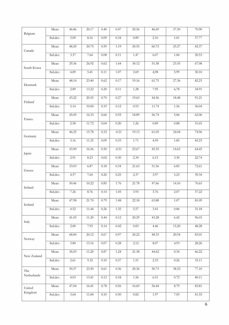
In Table 4 we present the two final specifications of the EAM approach given by models 2 and 3. In

both specifications we consider Fb(.) instead of BB. The latter is the full version of eq. (3’) where

dummies concerning the economic financial crisis and the leader/follower innovation country position

are both included, the former does not consider Dc. In particular, the inclusion in models 2) and 3) of

the dummies for the structural break of financial crisis revealed to be alternative in terms of statistical

significance with the trend variable - years since broadband introduction - considered in Model 1. As

said above, such a variable (TB) picks all the exogenous effects in the EAM specification, and so also

financial crisis effect, which now is highlighted more appropriately in models 2) and 3). However, as

expected, the lagged term slightly rises because the substituted variable - i.e., the trend - covered the

major part of the observed period. Therefore, in models 2) and 3), the lagged term now accounts also

for the dynamics not considered by new dummies. The broadband penetration rate coefficient is

undervalued in these final models even though highly significant. This is due to: a) the indirect

estimation adopted - i.e., after the logistic stage-, which implies an additional variability and affects

coefficients’ standard error; b) the consideration of financial crisis, which reduces the role of the new

technologies in favor of the more traditional resources for growth. In Table 5 we show the long run

parameters, the mean time lags and the speeds of adjustment. Coherently with point b), we note that, at

least in the long run, 3rd level Human capital is slightly undervalued in models 2) and 3) and, conversely,

the coefficient of Fixed capital formation rate shows an increase in the positive effect on GDP (in the

case of model 2) or a very similar coefficient with respect to the first model (in the case of model 3);

Workforce growth rate coefficient, finally, exhibits a smaller negative value.

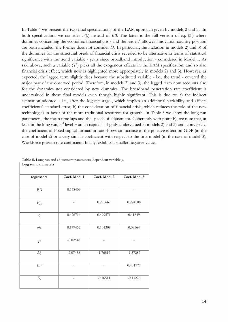
Table 5. Long run and adjustment parameters, dependent variable yt

long run parameters

regressors Coef. Mod. 1 Coef. Mod. 2 Coef. Mod. 3

BB 0.558409 - -

Fb,t - 0.295667 0.224108

st 0.426714 0.499571 0.41849

hkt 0.179452 0.101308 0.09564

TB -0.02648 - -

∆lt -2.07458 -1.76517 -1.37287

LF - - 0.481777

Dc - -0.16511 -0.13226

15

Constant 5.542737 5.202138 4.380019

adjustment parameters

(Speed of adj.) 0.35157 0.20956 0.23212

Mean time lag 2.844384 4.771903 4.308116

From Table 5 we can check that accounting properly for the period of financial crisis rises the mean

time lag and consequently the period of adjustment. This is reasonable considering the difficulty of

growing during the crisis and the relatively bigger effects –i.e., compared to a lower economy

dimension- of new investments, which implies a longer process of adjustment.

7. Policy implications

We introduced this research by asking ourselves the reasons why modern countries should be

interested in facilitating the deployment of broadband communication infrastructures. In this section

we try to address this specific question by expounding some of the possible policy implications deriving

from the estimations obtained. We have just considered in Table 5 the long run parameters, the speeds

of adjustment and the mean time lags of the models studied, which helps us study the effects on output

growth over time. However, in order to be more effective, we can now qualify more explicitly the

changes in output per capita obtainable in the short, medium and long run.

From tables 5, 4 and 3 we find the impact of a change in broadband penetration rate on GDP per

capita for the OECD countries considered in the long and in the short run. However, since these ones–

and especially the long run - are not precise concepts in terms of time interval we also compute the

effect within the mean time lag, which is the amount of time expected to exert a relevant impact on the

dependent variable following a change in the independent one. More specifically, this period is given by

2.84, 4.78 and 4.3 years, respectively for the first, second and third model estimated, which corresponds

to what is commonly considered as the medium run. We now show that “relevant effect” means about

the 63% of the discrepancy between the actual and the target value, that in our case - given the linear

model considered- is the increase in the broadband penetration rate (BB) multiplied by its long run

parameter. So, by writing in a more compact form the expression (3)

(13) 1

ss

it it ity y y

and making use of the suitable change of variable s=t-, we may write (13) in terms of its continuous time equivalent form exponential lag distribution8

(14)

0

tt sss ss

it t sy e y d e y ds

8 The exponential lag distribution (14) is the continuous counterpart of the discrete development of (13) in terms of

geometric lag distribution, or Koyck distributed lag equation, with e being the exponential distribution (see Kenkel,

1974).

16

from which, in order to discern how quantitatively relevant is the effect on which we are investigating –

i.e., BB - within the mean time lag, we impose and obtain

(15)

00

0.632

tt s

it BB BB BB BB

t

y BB e ds BB e d BB e BB

where BB is the long run, or steady state, parameter of BB in Table 5.

This refinement represents, compared to existing literature, a relevant implication of our estimation

strategy. The EAM approach besides rigorously taking into account the adjustment process towards the

equilibrium and coping with non linearity, indeed allows to measure, for each country in the short,

medium and long run, the impact on GDP per capita of a percentage increase of BB. So, in the

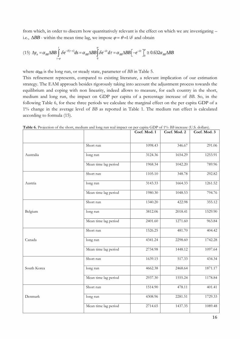
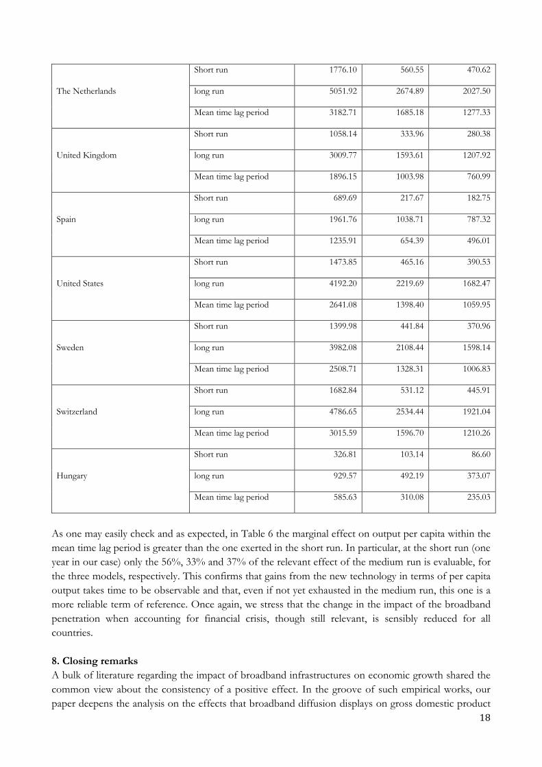
following Table 6, for these three periods we calculate the marginal effect on the per capita GDP of a

1% change in the average level of BB as reported in Table 1. The medium run effect is calculated

according to formula (15).

Table 6. Projection of the short, medium and long run real impact on per capita GDP of 1% BB increase (U.S. dollars).

Coef. Mod. 1 Coef. Mod. 2 Coef. Mod. 3

Australia

Short run 1098.43 346.67 291.06

long run 3124.36 1654.29 1253.91

Mean time lag period 1968.34 1042.20 789.96

Austria

Short run 1105.10 348.78 292.82

long run 3143.33 1664.33 1261.52


Belgium

Short run 1340.20 422.98 355.12

long run 3812.06 2018.41 1529.90


Canada

Short run 1526.25 481.70 404.42

long run 4341.24 2298.60 1742.28


South Korea

Short run 1639.15 517.33 434.34

long run 4662.38 2468.64 1871.17


Denmark

Short run 1514.90 478.11 401.41

long run 4308.96 2281.51 1729.33


17

Finland

Short run 1297.65 409.55 343.85

long run 3691.02 1954.33 1481.33


France

Short run 996.46 314.49 264.04

long run 2834.32 1500.72 1137.51


Germany

Short run 1106.68 349.28 293.24

long run 3147.84 1666.72 1263.33


Japan

Short run 1035.16 326.70 274.29

long run 2944.38 1558.99 1181.68


Greece

Short run 2697.44 851.33 714.75

long run 7672.55 4062.47 3079.25


Ireland

Short run 723.83 228.45 191.80

long run 2058.85 1090.12 826.29


Iceland

Short run 1474.32 465.31 390.66

long run 4193.54 2220.40 1683.01


Italy

Short run 591.92 186.81 156.84

long run 1683.64 891.46 675.70


Norway

Short run 1866.21 588.99 494.50

long run 5308.21 2810.60 2130.36


New Zealand

Short run 591.51 186.68 156.73

long run 1682.47 890.84 675.23


18

The Netherlands

Short run 1776.10 560.55 470.62

long run 5051.92 2674.89 2027.50


United Kingdom

Short run 1058.14 333.96 280.38

long run 3009.77 1593.61 1207.92


Spain

Short run 689.69 217.67 182.75

long run 1961.76 1038.71 787.32


United States

Short run 1473.85 465.16 390.53

long run 4192.20 2219.69 1682.47


Sweden

Short run 1399.98 441.84 370.96

long run 3982.08 2108.44 1598.14


Switzerland

Short run 1682.84 531.12 445.91

long run 4786.65 2534.44 1921.04


Hungary

Short run 326.81 103.14 86.60

long run 929.57 492.19 373.07


As one may easily check and as expected, in Table 6 the marginal effect on output per capita within the

mean time lag period is greater than the one exerted in the short run. In particular, at the short run (one

year in our case) only the 56%, 33% and 37% of the relevant effect of the medium run is evaluable, for

the three models, respectively. This confirms that gains from the new technology in terms of per capita

output takes time to be observable and that, even if not yet exhausted in the medium run, this one is a

more reliable term of reference. Once again, we stress that the change in the impact of the broadband

penetration when accounting for financial crisis, though still relevant, is sensibly reduced for all

countries.

8. Closing remarks

A bulk of literature regarding the impact of broadband infrastructures on economic growth shared the

common view about the consistency of a positive effect. In the groove of such empirical works, our

paper deepens the analysis on the effects that broadband diffusion displays on gross domestic product

19

(per capita), on the base of a panel composed by a sample of 23 OECD countries over 17 years (1996-

2012). Overall, the all results confirm that broadband diffusion is both statistically significant and

positively correlated with the growth of real GDP per capita. This result is robust even after accounting

for fixed capital formation, human capital, workforce growth rate, years since BB introduction, national

ability to innovate (leader/follower) and structural breaks (crisis). In other terms, given the ability to

foster economic growth, there are high incentives for public policy interventions (on both sides of

demand and supply) oriented to enhance BB diffusion and, in particular, to push up for the full

deployment of upgraded new communication networks (UWB).

In achieving these results we implemented a dynamic growth model which considers the adjustment

process towards the equilibrium based on instrumental variables. This allows for both testing and

assessing the long run or short run relations of the estimated equation and overtake the endogeneity

problem. Moreover, in considering that an adjustment process is in force, we can cope also with the

nonlinear effects of BB on GDP taking into account the time adaption needed to implement new

technologies (Holt and Jamison, 2009).

Acknowledgments

We are grateful to the University of Rome “La Sapienza” and MIUR for funds provided to support this research. We also wish to thank Stefano Fachin and the participants to the 17th Annual Infer Conference 2015, where this paper was presented, for helpful comments and suggestions.

References:

Aghion, P.; Howitt, P. (1992): “A Model of Growth through Creative Destruction, Econometrica, vol. 60,

n. 22, pp. 323-351.

Arellano, M.; Bond, S. (1991): “Some Tests of Specification for Panel Data: Monte Carlo Evidence and

an Application to Employment Equations”; Review of Economic Studies, vol. 58, n. 2, pp. 277-297.

Baltagi, B.H. (2005): Econometric Analysis of Panel Data, 3rd ed.; Wiley, New York

Brynjolfsson, E. (1993): “The productivity paradox of information technology”; Communications of the

ACM, vol. 36, n. 12, pp. 66-77.

Brynjolfsson, E.; Yang, S. (1996): “Information Technology and Productivity: A Review of the

Literature”; Working Paper, MIT Sloan School of Management.

Breitung J, Pesaran MH (2008) Unit roots and cointegration in panels. In: Matyas L, Sevestre P (eds)

The 818 econometrics of panel data. Kluwer, Dordrech

Comin, D.; Hobijn, B.; Rovito, E. (2006): “Five facts you need to know about technology diffusion”;

NBER Working Paper, n. 11928, National Bureau of Economic Research, January 2006.

Cradall, R.; Lehr, W.; Litan, R. (2007): “The Effects of Broadband Deployment on Output and

Employment: A Cross-sectional Analysis of U.S. Data”; Issues in Economic Policy, n. 6, The Brookings

Institution.

Czernich, N.; Falck, O.; Kretschmer, T.; Woessmann, L. (2011): “Broadband Infrastructure and

Economic Growth”; The Economic Journal, vol. 121 (5), pp. 505-532.

Everett, M.R. (1995): Diffusion of Innovations, 5th ed.; Free Press – Simon & Schuster, New York.

Fisher, J.: Pry, R.A. (1971): ”Simple Substitution Model of Technological Change”; Technological

Forecasting and Social Change, n. 3, pp. 75-88.

20

Fisher, J.C.; Pry, R.H. (1971): “A Simple Substitution Model of Technology Change; Technological

Forecasting and Social Change, vol. 3 (…), pp. 75-88.

Geroski, P.A. (2000): “Models of technology diffusion”;.Research Policy vol. 29 n. 4-5, pp. 603-625.

Gillet, S.E.; Lehr, W.H.; Osorio, C.A.; Sirbu, M. (2006): “Measuring Broadband’s Economic Impact”;

Final Report, Economic Development Administration ,U.S. Department of Commerce.

Grosso, M. (2006): “Determinants of broadband penetration in OECD nations”; Australian

Communications Policy and Research Forum.

Gruber, H. (2001): “Competition and innovation: The diffusion of mobile telecommunications in

Central and Eastern Europe”; Information Economics and Policy, vol. 13, n. 1, pp. 19-34.

Gruber, H.; Verboven F. (2001). “The evolution of markets under entry and standards regulation: The

case of global mobile telecommunications”; International Journal of Industrial Organization, n.19, pp.1189-

1212.

Holt, L.; Jamison, M. (2009): “Broadband and contributions to economic growth: Lessons from the US

experience”; Telecommunications Policy, n. 33, pp. 575-581.

International Telecommunication Unit (2011): “Measuring the Information Society, ITU, Switzerland.

Kenkel, J. L., (1974), “Dynamic Linear Economic Models”, Gordon and Breach, New York.

Kim, Y.; Kelly, T.; Raja, S. (2010): “Building broadband: Strategies and policies for the developing

world”; Global Information and Communication Technologies (GICT) Department, World Bank, January 2010.

Kretschmer, T. (2012), “Information and Communication Technologies and Productivity Growth: A

Survey of the Literature”, OECD Digital Economy Papers, No. 195, OECD Publishing.

Lee, S.; Brown, J.S. (2008): “The Diffusion of Fixed Broadband: An Empirical Analysis”; Working Paper

NET, The Networks Electronic Commerce and Telecommunications Institute, n.8-19, September

2008.

Lee, S.; Marcu, M.; Lee, S. (2011): “An empirical analysis of fixed and mobile broadband diffusion”;

Information Economics and Policy, vol.23, n.3-4, pp. 227-233.

Lucas, R.E. (1988): ”On the mechanics of Economic Development”; Journal of Monetary Economics, n. 22,

pp. 3-42.

Maggi, B, (2014), “ICT Stochastic Externalities and Growth: Missed Opportunities, Beyond

Sustainability, or What?”; DSS Empirical Economics and Econometrics Working Papers Working

Papers Series n. 2014/4.

Mankiw, N.G.; Romer, D.; Weil, D.N. (1992): “A contribution to the empirics of economic growth”;

Quarterly Journal of Economics, vol.107, n. 2, pp. 407-437.

Meyer, P.S.; Yung, J.W.; Ausubel, J.H. (1999): “A Primer on Logistic Growth and Substitution: The

Mathematics of the Loglet Lab Software”; Technological Forecasting and Social Change, vol. 61 (3), pp. 247-

271.

Nelson, R.R.; Phelps, E.S. (1966): “Investment in Humans, Technological Diffusion, and Economic

Growth”; The American Economic Review, vol. 56, n. 1/2, pp. 69-75.

OECD (2009): “The Role of Communication Infrastructure Investment in Economic Recovery”;

Working Party on Communication Infrastructures and Services Policy, Organization for Economic Cooperation

and Development, May 2009.

Romer, P.M. (1990): “Endogenous technological change”; Journal of Political Economy, n. 98, pp. 71-102.

Romer, P.M. (1994): “The Origins of Endogenous Growth”; The Journal of Economic Perspectives, n. 8, pp.

3-42.

Singh, S.K. (2008): “The diffusion of mobile phone in India”; Telecommunications Policy n. 32, pp. 642-

651.

21

Solow, Robert M. (1957). "Technical Change and the Aggregate Production Function"; Review of

Economics and Statistics, vol. 39, n. 3, pp. 312-320.

Solow; R.M. (1956): "A Contribution to the Theory of Economic Growth"; Quarterly Journal of

Economics, vol. 70, n. 1, pp. 65-94.

Stryszowski, P. (2012), “The Impact of Internet in OECD Countries”, OECD Digital Economy Papers, n.

200, Organization for Economic Cooperation and Development, June 2012.

van Ark, B.; Inklaar, R. (2005): “Catching up or getting stuck? Europe’s trouble to exploit ICT’s

productivity potential”; Research Memorandum GD-79; Groningen Growth and Development Centre;

September 2005.

von Hayek, F.A. (1945): “The Use of Knowledge in Society”; American Economic Review, vol.35, n. 4, pp.

519-530.

Oz, E. (2005): “Information technology productivity: in search of a definite observation”; Information

& Management, n. 42, pp. 789-798.

Flamm, K.; Chaudhuri, A. (2007): “An analysis of the determinants of broadband access”;

Telecommunication Policy, vol. 31, n. 6-7, pp. 312-326.

Documents

Measuring (in a time of crisis) the impact of broadband ... · Sezione di Statistica Economica ed Econometria Angelo Castaldo Alessandro Fiorini Bernardo Maggi Measuring (in a time